forecasting nigeria gdp growth rate using a dynamic factor ... forecasting gdp.pdf · common factor...

FORECASTING NIGERIA GDP GROWTH RATE USING

A DYNAMIC FACTOR MODEL IN A STATE SPACE FRAMEWORK

CENTRAL BANK OF NIGERIA

RESEARCH DEPARTMENT, CENTRAL BANK OF NIGERIA

© 2015 Central Bank of Nigeria

Central Bank of Nigeria Research Department 33, Tafawa Balewa WayCentral Business District P.M.B. 0187Garki, AbujaWebsite: www.cbn.gov.ng

Tel: +234(0)94635900

The Central Bank of Nigeria encourages dissemination of its work. However, the materials in this publication are copyrighted. Request for permission to reproduce portions of it should be sent to the Director of Research, Research Department, Central Bank of Nigeria, Abuja.

A catalogue record for publication is available from the National Library.

ISBN - 978-978-951-926-2

CONTRIBUTORS Charles N. O. Mordi Michael A. Adebiyi Adeniyi O. AdenugaMagnus O. Abeng Adeyemi A. Adeboye Emmanuel T. AdamgbeMichael C. OnonugboHarrison O. Okafor Osaretin O. Evbuomwan

List of Figures............................................................................... iii

List of Tables................................................................................ iii

Non-Technical Summary ........................................................... iv

CHAPTER ONE ............................................................................. 1

1.0 Introduction ...................................................................... 1

CHAPTER TWO.............................................................................. 4

2.0 Brief Review of Relevant Related Literature.................. 4

CHAPTER THREE............................................................................10

3.0 Stylized Facts on the Nigerian Economy .......................10

CHAPTER FOUR.............................................................................13

4.0 Methodology....................................................................13

4.1 Determination of Variables for Inclusion in the in the

Dynamic Factor Model .................................................. 15

4.2 Estimation Technique...................................................... 22

4.2.1 Kalman Filtration.............................................................. 22

4.2.2 Growth Dynamic Factor Model..................................... 24

4.2.3 Forecasting Growth......................................................... 26

CHAPTER FIVE............................................................................... 27

5.0 Empirical Results ............................................................... 27

5.1 Forecasting the GDP Growth: the Estimated

Common Component..................................................... 30

CHAPTER SIX................................................................................. 34

6.0 Conclusion ...................................................................... 34

Reference.................................................................................... 36

Appendix 1: Variable Definitions

Appendix 2: The Markov Chain Model

ii

Table of Contents

List of Figures

Figure 1: Switching State Probabilities for Annualised

Real Output Growth Rates........................................... 11

Figure 2: Dynamic Correlation of GDP growth with

Selected Macroeconomic Variables......................... 16

Figure 3: Filtered State Estimate of the Common Factor...........29

Figure 4: Composite Leading Indicator and GDP Growth....... 31

Figure 5: GDP Growth Rate - Actual and Forecast (%) ............ 33

List of Tables

Table 1: Summary Results of the Markov Switching Model..... 12

Table 2: Cyclical Correlation of GDP Gap with Some De-

trended Macroeconomic Variables........................... 19

Table 3: Evaluation of the In-Sample Forecast Performance

of the Models................................................................. 28

Table 4: Estimated Factor Loadings........................................... 28

iii

Today, the objective of the CBN like any other central banks is the

attainment of monetary and price stability usually based on

predetermined targets. According to Arestis (2007), the management

of inflation has shifted from the attempts to stabilise it around targets to

efforts at anchoring inflation expectations. Understanding of

economic outlook provides vital information on the evolution of future

inflation and helps central banks in their price stability mandates. In the

literature, several methods such as the static component, dynamic

component and/or both have been applied to forecast economic

activity. A number of these techniques are fraught with some

challenges: first, they could lead to large forecasting errors; second,

such forecasts could mislead economic agents who act based on

decision made by monetary and fiscal authorities.This approach allows

for the modelling of unobserved components in the time series with the

advantage of improving the quality of forecasts germane to central

banks' capacity in implementing forward-looking monetary policy.

Thus, this study employed a dynamic factor model to forecast gross

domestic product (GDP) growth rate for Nigeria. The justification for this

approachis anchored on its ability to extract the underliningfactors

required in generating robust and reliable forecast of GDP. The

common factor for Nigeria's GDP was derived based on six

macroeconomic variables, including GDP growth rate, growth in

money supply, credit to the core private sector, government revenue,

government expenditure and crude oil production. The forecast

period covered 2014Q2 to 2015Q4.

The forecast showed a real GDP growth rate which generally remained

above 6.50 per cent. From an actual growthrate of 6.54 per cent in

2014:Q2, output growth was forecasted to rise to 6.93 per cent in

2014:Q3. Nonetheless, a modest slowdown was predicted towards the

iv

Non-TechnicalSummary

FORECASTING NIGERIA GDP GROWTH RATE USING A DYNAMIC FACTOR MODEL IN A STATE SPACE FRAMEWORK

end of 2014 and throughout 2015. GDP growth rates for 2015:Q2 and

2015:Q4 were forecasted as 6.83 and 6.75 per cent, respectively. The

study also identifiedcomposite leading indicatorsforpeaks and troughs

in the real GDP growth. Further analysis suggesteda persistence

ofgrowth contraction which lasted about 7.4 months, while the higher

growth regime continued for approximately 4.6 months.Thus, in a

dynamic economy like Nigeria, the need to regularlyfine-tune this

framework becomes imperative.

v


The need for a more consistent and accurate GDP forecast

for the conduct of forward-looking monetary policy is quite

fundamental. This is because the availability of real-time

data is crucial to determine the initial conditions of economic

activity on latent variables such as the output gap to make

policy decisions. Central banks use available monetary policy

instruments to influence the volume and direction of monetary

aggregates, consistent with predetermined output and price

targets. In both developed and developing countries, a

traditional central bank reaction function is characterised by

price and output development. Thus, taking decisions about the

monetary policy rate without an estimate of the output gap is

tantamount to 'flying blind' and making unacceptably, large

errors and revisions that are uncertain

Several benefits can be derived from generating accurate now-

cast of GDP. First, without such reliable forecast, misleading

decisions could be taken with far-reaching consequences on

the set objectives and forward mis-guidance of economic

agents. Second, since output stabilisation is one of the key

objectives of the policy maker, accurate output forecast can

help to reveal the sacrifice ratio relative to other objectives, such

as inflation and exchange rate stability. Third, where structural

models are also used for simulation, GDP forecast can feed into

these models, thus, enriching mid-term forecast.

Although statutory agencies of government release values of

key macroeconomic variables such as output,they come with

some lag given the enormity of the data-generating process,

particularly the labourious and time-consuming as well as costly

1

Chapter One1.0 Introduction


field surveys. The lag in the release of actual numbers can be a

challenge to the policy makers. For Nigeria, it is even more

critical given that the GDP numbers comes with a two-quarter

lag. Also, over the last few decades, the economy has witnessed

sharp swings during the 1982, 1994 and 2008 global economic

crises periods. The pervasiveness of each of these domestic and

global phenomena has implications on the ability to measure

effectively potential and actual national output.Hence, a

forecasting framework is needed to effectively address the

challenge of understanding the current state of economic

activity for policy decisions.

Since there are several variables with mix frequencies (monthly,

quarterly, annually), such as money supply, inflation, stock

market capitalisation, whichhave strong correlation with output

growth that are readily available on a regular basis.It becomes

possible to generate GDP forecast by leveraging on the inherent

relationship among these variables. Schulz (2007) has shown that

financial and survey data are useful in the forecast of economic

activity. In the literature, several methods are used to summarise

these large data set for the purposes of forecasting such as the

static component, dynamic component and/or both have

been applied to forecast economic activity (Allen, 1997;

Anderson and Gascon, 2009; and Schulz, 2008). A number of

these techniques are fraught with some challenges (Stock and

Watson, 2002; Forni, et al., 2003; Schulz, 2008): first, they could

lead to large forecasting errors; second, such forecasts could

mislead economic agents who act based on decision made by

monetary and fiscal authorities.

2


Thus, this study employed a dynamic factor model (DFM) to

forecast gross domestic product (GDP) growth rate for Nigeria to

aid monetary policy decisions. This approach allows for the

modelling of unobserved components in the time series with the

advantage of improving the quality of forecasts germane to

central banks' capacity in implementing forward-looking

monetary policy. Particularly, this approach is anchored on its

ability to extract underlining factors among a set of

macroeconomic variables that contain information about the

latent state of the economy that can be used in generating

robust and reliable GDP forecast. The DFM provide help to

addressing the paucity of real-time data. It also permits the

utilisation of a mixture of data frequencies in the determination of

the current state of the economy. More so, if disturbances

suggest absence of normality of the random variables, it gives

room for a re-specification of the errors in an autoregressive

scheme.

Following this introduction, chapter 2 focuses on the literature

review while chapter 3 espouses the stylized facts about business

and growth cycles. Chapter 4 covers the methodological issues

as the empirical results are considered in chapter 5 while chapter

6 concludes the study.

3


The extant literature has shown that without good forecast,

the conduct of forward-looking monetary policy would be

complicated and misleading. Highlighting the importance

of forecast in forward-looking monetary policy, Kugler et al.,

(2004) examined the effect of measurement errors in GDP on

inflation and growth volatility in Switzerland. The paper noted

that with measurement errors, monetary policy reacted very

strongly to noisy data if the weight on output growth targeting

becomes too big, as measurement errors have a strong impact

on the growth forecast but not on the inflation forecast.

This finding was consistent with earlier studies such as

(Orphanides, 2000, 2001) in the US; and Ehrmann and Smets

(2003) in the euro area. In the US an examination of real time data

for output gap for measurement errors showed that observed

measurement errors in the output gap, the neglect of which, they

claimed, might result in aggressive policy posture. Thus, errors

associated with forecasts in the output gap can be a problem for

forward-looking monetary policy. For the euro area, welfare

losses in the form of high output variability to measurement

problems were traced.

Clarida et al., (2000) argued that if monetary policy would rein in

future inflationary pressures, the role of accurate forecasts

becomes very germane. Consequently, the paper evaluated

forecasts from three central banks of England, Poland and Swiss

in forward-looking Taylor rules to ascertain the forward looking

nature of their monetary policy decisions. The findings confirmed

that the sampled central banks were forward looking. The

4

Chapter Two2.0 Brief Review of Relevant Related Literature


1 Broadly speaking, models for economic forecasting can be classified into two groups - time series models and structural models. Time series models are mainly statistical, based on historical developments, traditionally with just a fewvariables and very little, if any, economic content. In structural models, on the other hand, economictheory is used to specify the relationships between the variables, which can be done either by estimationor by calibration.

intuition of this result reflects the necessity of generating key

forecasts in the objective function of the central bank for a

forward-looking monetary policy.

In terms of implementing forecast, the recognition of GDP series

as a veritable input for monetary policy formulation and

implementation has led to the adoption of several approaches

(structural and time series) in economic literature to forecast the

series (see Fenz, Schneider and Spitzer, 2004; Schumacher, 2005;

Schulz, 2007; Benkovskis, 2008; Branimir and Magdalena,

2010).The structural models have transited from the Cowles

Commission type of models to the more recent dynamic

stochastic general equilibrium (DSGE) models. The Cowles

Commission models were largely criticised for being ad hoc,

policy variant (Lucas critique) and the lack of micro-foundations

(see Mankiw, 1991, 2006; Woodford, 1999; and Goodfriend, 2007).

Earlier time series models were the ARIMA models based on Box-

Jenkins (1976) approach. In the recent times, the ARIMA models

are usually found in studies as benchmark models against which

other models are evaluated. A major limitation of the ARIMA

model is that it can only be used to predict itself.

This approach was extended in a multivariate application in the

vector autoregressions (VARs) following Sims (1980). Studies by

Stock and Watson (2001) have shown that VARs have been

successful in forecasting. In the class of time series models was the

5


1

extension of the VARs by applying larger scale Bayesian VARs as

shown the works of Litterman (1986), Sims (1993) and Sims and Zha

(1986).BVARs allows for the inclusion of limited variables and with

their lags. Again, Bayesian VARs impose some restrictions on the

model coefficients, thus, helping to reduce the dimensionality

problem of VARs, resulting in more accurate forecasts. A major

drawback of the VAR and BVAR among other time series model

used for forecasting is it inability to include large number of

variables.

In the second class of time series models are the Unobserved

Components (Harvey, 2006). This class warehouses the large

averaging and empirical Bayes methods; and the factor models

in the spirit of Stock and Watson (2006). Thus, in the recent

literature, the factor models, which allow the inclusion of large set

of latent variables was developed to deal with such challenges

(Schumaber, 2005). Factor models such as the static component

Stock and Watson (2002) and the dynamic principal component

models in the time domain as in Doz et al., (2006 and 2007) and

dynamic principal components in the frequency domain, as in

Forni et al (2000 and 2004) have become prominent in the

forecasting of GDP given their ability to include unobserved

components to predict the future path of GDP.

Fenz, Schneider and Spitzer (2004) made a forecast of Austrian

real GDP by combining the forecast of unobserved components

and a dynamic factor model. A unique feature of the model is

the aggregation procedure used to derive quarterly GDP growth

rates. Kalman filter technique was used to estimate and extract

the unobserved GDP growth rate series. Basing their estimation

6


on an autoregressive term and exogenous conjugal indicators,

the authors noted the short-term out-of-sample forecast of real

GDP in Austria performing significantly better than the

benchmark models. Similarly, the model accurately predicts the

latest data relative to the first data release.

For the US economy, Allen and Pasupathy (1997) adopted the

state space representation in forecasting the fiscal and

monetary control (exogenous) variable. They specified a linear

relation between state variables, allowing for time variation using

a recursive least squares with exponential forgetting factors and

ordinary least squares estimations. The forecast result show that a

one-step-ahead recursive least squares estimates tracks the

actual annual monthly GDP growth rates perfectly while its

algorithm shows a better performance in the out-of-sample

forecast especially for state variables that exhibit the greatest

cyclical variation.

Schulz (2007) applied the small scale state space and the large

scale static principal components models propounded by Stock

and Watson (1991, 2002) to Estonian data to forecast real

economic growth and then benchmark the result against other

forecasting models. Estimating the model with maximum

likelihood and the Kalman filter procedure, the result suggest the

relevance of financial data, particularly growth in monetary

aggregate and investment and some survey type data, over

other economic data in forecasting the Estonian economic

trajectory. The model could not, however, identify classical

business cycle with booms and recessions in Estonia.

7


Benkovskis (2008) used coincident information from monthly

industrial production, retail trade, broad money aggregate, and

confidence indicators to estimate a short-term forecast of

Latvia's real GDP growth in a state space representation. The

study used quarterly univariate forecasting (bridge) equations

incorporated into state space framework containing real GDP

and 28 vintage of quarterly real GDP. The result showed that the

bridge equations that include broad money aggregates

performs better than the ARIMA models even though both

models provide valuable information when broad money

aggregatesare included.

Recently, one of the most applied real GDP forecasting

techniques in analyzing time dependent system has been the

dynamic factor models in state space representation owing

largely to its flexibility in information extraction (see Anderson and

Gascon, 2009; Camacho et al., 2013; and Hindrayanto et al.,

2014 ).

Anderson and Gascon (2009) employed the state space

framework in estimating the 'true' unobserved measure of total

output in the US economy. The objective (is) was to estimate the

'true' value of real output for use in the construction of trend-like

measures of potential output. Using revised statistics with recent

data vintage in a state space framework to extract estimates of

the 'true' series, the model result suggested an improved real

GDP closer to 10 per cent reduction in uncertainty. In terms of

forecast accuracy of a state space framework, these results

were consistent with those in Baek (2010).

8


Camacho et al., (2013) adopted a small scale dynamic factor

model in forecasting Argentine's real GDP using mixed frequency

vintage economic data. The model was able to capture the

turning points of the highly volatile Argentine's GDP growth path

mimicking the history of the country's business cycle. In addition,

the model's precision in producing reliable back-cast and now-

cast real data was ascertained as it explained about 89 per cent

of the volatility in Argentine's real GDP growth.

In terms of forecast evaluation using the root mean squared error

and the mean absolute error, Jovanovic and Petrovska (2010)

gauged the forecast ability of six different short-term modelsfor

the Macedonian economy including the Kalman filter. The model

result indicated that the static factor model outperforms other

models, suggesting that models with large data sets improved

forecast ability. In a similar study for the Euro area, Hindrayanto et

al., (2014) found the dynamic factor models to be superior over

other models showing a forecast precision of about 77 per cent in

the mean squared error.

The dynamic factor models have been applied in Germany,

Australia and Macedonia. There is yet, no evidence of the

application of dynamic component model in Africa.

9


To further understand the cyclical properties of output growth the

regime switching behaviour is investigated in line with Hamilton

(1989) and Schulz (2008). This enabled us disaggregate the state

of the economy growth cycles into regimes as per whether

growth rate was rising (the state of output acceleration i.e.

“growth expansion”) or declining (the state of output slowdown

i.e. “growth contraction”). Hence, a 2-regime multivariate

Markov Chain model is fitted where GDP growth (Hence, a 2-

regime multivariate Markov Chain model is fitted where GDP

growth is allowed to follow an AR(1) process.

The first regime indicates growth contraction and captures

approximately about three cyclical periods in economic activity

in the last one and half decade. These are observable for the

periods, 2004-06, period of banking crisis and consolidation; 2007-

09, the impact of the global economic and financial crises which

slowed growth; and for the most part, from 2010 to date, that

growth moderated to low growth levels.

The estimated regime switching intercepts, government

revenue, government expenditure, crude oil production and

core credit to the private sector, are the drivers in explaining the

growth cycles. An analysis of the matrix of transition probabilities

shows that the two regimes are relatively not permanent, since

the estimated probability is less than one.

Figure 1 characterised Nigeria's growth cycles for the period

2001:Q1 to 2014:Q2 and showed that incidences of retarding

2 See appendix for the specification of the Markov Chain Model.

10

Chapter Three3.0 Cyclical Properties of Output Growth in Nigeria


2

growth rate occurred more frequently than of growth expansion.

Moreover, as observed in the middle panel that chart, output

decelerations seemed to persist for longer periods than growth

expansions. While growth contraction does not connote

recession (or an absolute decline in output) a sustained

deceleration could eventually cause the economy to shrink. The

estimated transition probability matrix and the associated

ergodic probabilities cyclical states are presented in Table 1.

Figure 1 : Switching State Probabilities for Annualised Real Output Growth Rates

11


There is an 86.5 per cent probability of remaining in regime 1, a

contraction, which is higher than the 78 per cent probability of

staying in the expansion state, which implies that the contraction

regime is more persistent than expansion regime. Also, the

transition probability from a regime of low growth towards a

higher growth is 13.5 per cent, lower than the 21.6 per cent

probability of exiting a high growth towards lower growth.

Further, the ergodic probabilities indicate that on average

contraction lasts about 7.4 months, while the higher growth

regime continues for approximately 4.6 months, suggesting more

periods of growth contraction.

Table 1: Summary Results of the Markov Switching Model

Transition matrices Expected duration

1 2 Regime

1

0.865

0.135 Regime 2

0.216

0.784

Regime 1 Regime 2 All periods

7.39

4.62

12


4.1 Determination of Variables for Inclusion in the

Dynamic Factor Model

In many cases, macroeconomic variables could exhibit co-

movements with phase-shifts across a time domain. Hence, it is

important to measure these inter-temporal cross-correlations at

different lags and leads. Conventionally, a rolling cross-

correlation, termed dynamic correlations, is computed between

a reference series and an array of macroeconomic series at

predetermined time band. In this study, the dynamic correlation

of a reference series other series at lag/lead is determined

as:

and

The resulting solution gives a scalar quantity, , at time and the

lag/lead of series . In the immediate discussion, dynamic

correlations are determined between GDP growth, as the

reference series, and some selected macroeconomic variables

over a 6-lead-lag time domain. This provides some information

regarding the relative importance of individual variables and the

comparative prominence of backward- versus forward-looking

expectation.

Figure 1, depicts the charts of the dynamic correlations with

reference to GDP. Panel (a) of that figure plots the inter-temporal

co-movements of various interest rate variables with GDP growth.

The plots showed a generally downward sloping trend from lags

to leads. The implication of this is that not only would a

contemporaneous rise in interest rates lower output growth,

expected increases would decelerate aggregate demand. The

13

Chapter Four4.0 Methodology


co-movements of lagged interest, however, showed mixed

results. While policy and lending rates maintained a negative

coefficient, deposit rate exhibited a positive value between lags

3 and 6. This is not unexpected, as increases in deposit rates

would increase future consumption and aggregate demand.

Examination of that chart indicates that interest rate on 3-month

deposits correlated more with GDP growth rate, on the average,

over the leads and lags while monetary policy rate had the least

average coefficient.

The quantity theory of money suggests a positive relationship

between money and output, ceteris paribus. In panel (b) this

relationship was examined. Monetary aggregates, therein,

exhibited wave-like cycles of dynamic correlations, which were

predominantly negative; suggesting a largely inverse

relationship between monetary gaps and output growth. The

chart generally suggested that monetary overshoots are

detrimental to economic growth whether in a forward- or

backward-looking framework. Comparing leads and lags, the

plots indicated that backward adjustments were considerably

more relevant for GDP growth, with respect to money. The largest

but negative correlations occurred in the second lag. In the

contemporaneous, positive co-movements are seen for base

money and narrow money, albeit weakly.

Liquidity management actions of the CBN do not only affect

banks' ability to create credits but could impact on aggregate

demand. This informs the CBN's use of CRR both as a prudential

instrument and a monetary policy tool. Panels (c) and (d)

showed the dynamic correlations of output growth with bank

3

3 Due to the inter-temporal substitution and income effect in household utility function4 Monetary gaps are defined as the difference between monetary growths and the respective monetary growth targets determined via a process of financial programming.

14


4

reserves and domestic credits. The relationships plotted in panel

(c) suggested that rising reserve requirement could retard

economic growth given the negative correlation coefficients

over the leads and lags. While the positive coefficients for excess

reserve indicate that it could heighten aggregate demand,

create excess demand, accelerate output growth and

overheat the economy. The chart suggested that past

adjustments of the CRR (particularly in the second lag)

maintained a slightly larger relationship with contemporaneous

GDP growth than did expected adjustments.

Similarly, past outcomes of excess reserve had more relationship

with GDP growth, albeit marginally, than expected future

outcomes. In panel (d) credits are seen to relate positively with

output growth over leads and lags. The dynamic correlations of

NDC and CPS trended upward from lag to lead, suggesting that

future expectations of credit is more important for output growth

than past outcomes of credit. Besides, NDC is seen to generally

correlate more with output growth than did credit to private

sector. This could be indicative of the overriding importance of

government credits to the economy.

15


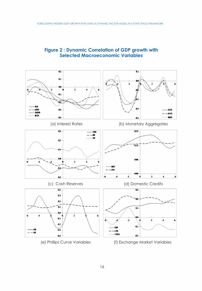
Figure 2 : Dynamic Correlation of GDP growth with Selected Macroeconomic Variables

(a) Interest Rates (b) Monetary Aggregates

(c) Cash Reserves (d) Domestic Credits

(e) Phillips Curve Variables (f) Exchange Market Variables

16


The plots in panel (e) showed the relationships of GDP growth with

inflation and unemployment rates. The dynamic correlations

were somewhat perverse of most leads and lags. For instance,

unemployment rate could be seen to maintain fairly even

positive inter-temporal correlations with GDP growth.

Theoretically, economic expansion is posited to diminish

unemployment rate; hence, an expected negative relationship

is expected. Though the positive sign is a puzzle, it nonetheless

highlights the idiosyncratic nature of the Nigerian economy. This

peculiarity of the economy is further illustrated in the output-

inflation relationship, which is expected to be positive across

leads and lags. However, the inflation plot in panel (e) showed a

meandering of the dynamic correlation coefficients from positive

to negative values over the leads and lags. Negative coefficients

could be seen at and around the contemporaneous period, i.e.

between lag 2 and lead 1. The depicted inverse relationship is

suggestive of the dominance of aggregate supply on

contemporaneous and near-term inflation rate. This aggregate

supply claim could be reinforced by the positive coefficients

recorded after lag 2. In this regard, inflationary outcome relates

directly with economic expansion, which suggested that rising

prices (via expected profits) encourages production and bolsters

aggregate supply. It is not clear, however, whether lags

outperformed leads for the inflation correlations.

In panel (f), external reserves could be seen to have a positive

and near symmetric dynamic correlation with GDP growth over

leads and lags. The level of exchange rate showed an upward

sloping positive relationship, indicating the rising importance of

expected exchange rate on output growth. However, exchange

17


rate depreciation (USD%) depicted negative coefficients for

contemporaneous and lead dynamic correlations. This indicated

that sizeable current and expected future depreciations of the

naira-dollar exchange rate related inversely with economic

expansion. Conversely, past depreciations, between lags 1 and

3, related positively with output growth. Hence, keeping

expected depreciation of the exchange rate low could provide

output stabilisation.

Next, conducting a similar analysis with transformed and

enlarged data series attempts are made to determine the short-

term leading indicators for real GDP. A log-transformed real GDP

is de-trended using the Hodrick-Prescott (HP) filter to derive the

output gap as a new reference series. Cycles of other suitable

variables are also derived in this way. The leading indicators are

determined from the dynamic correlations of 52 variables with

the GDP gap. These are shown in Table 2.

Cross correlation coefficients are compared for the entire series

within individual lead/lag. The top six variables with the highest

coefficients in each lead/lag of the time domain are highlighted.

For instance in the time domain the six leading indicators are

de-trended real personal disposable income (-0.37), de-trended

index of manufacturing production (+0.34), de-trended real

personal consumption expenditure (-0.33), de-trended savings

deposits of banks (+0.28), de-trended government revenue

(-0.28) and de-trended government expenditure (-0.19).

Thereafter, a latitudinal comparison is conducted on each row to

determine which variables appeared in the top six most

frequently. These are thus identified as the leading indicators of

economic cycles.

18


Table 2 : Cyclical Correlation of GDP Gap with Some De-trended Macroeconomic Variables

Kkmax Number

-6 -5 -4 -3 -2 -1 0 +1 +2 +3 +4 +5 +6

1 ASI_CYC

0.02

0.02

-0.09

-0.12

0.02

0.02

-0.05

-0.09

0.06

0.07

0.00

-0.03

0.10

+6

0

2 BLTL_CYC

0.00

0.04

-0.02

-0.06

-0.06

0.00

-0.04

-0.08

-0.06

0.02

-0.02

-0.06

-0.04

+1

0

3 BM_CYC

-0.02

-0.36

0.13

0.24

-0.12

-0.41

0.16

0.31

-0.12

-0.42

0.19

0.36

-0.12

+3

6

4 CCPS_CYC

0.14

-0.10

-0.17

0.10

0.17

-0.11

-0.24

0.06

0.14

-0.12

-0.22

0.09

0.16

0

5

5 CG_CYC

0.01

0.09

0.10

0.01

-0.01

0.03

0.07

0.02 -0.02

0.01

0.04

-0.04

-0.08

-4

0

6 COP_CYC

-0.04

0.13

0.00

-0.14

-0.01

0.17

0.06

-0.12 0.00

0.17

0.05

-0.11

-0.01

-1, +3

2

7 CPD_CYC -0.05 0.33 -0.03 -0.16 -0.07 0.33 -0.02 -0.18 -0.08 0.35 0.00 -0.19 -0.12 +3 6

8 CPS_CYC 0.14 -0.10 -0.17 0.10 0.16 -0.11 -0.24 0.06 0.13 -0.12 -0.22 0.10 0.16 0 3

9 CRR_CYC -0.16 0.01 0.16 0.04 -0.13 0.00 0.12 0.01 -0.09 0.02 0.12 0.01 -0.10 -4 0

10 ER_CYC

0.07

-0.08

0.06

0.04

0.02

-0.17

0.05

0.09 -0.03

-0.21

0.06

0.10

-0.06

+3

2

11 EUR_CYC

0.10

0.01

-0.05

0.04

0.08

0.00

-0.05

0.00 0.05

0.00

-0.09

-0.08

0.00

-6

0

12 EXR_CYC

-0.03

-0.05

-0.09

0.00

-0.01

0.01

0.00

0.03

0.00

0.02

0.04

0.06

0.01

-4

0

13 GBP_CYC

0.03

0.06

-0.02

-0.01

0.06

0.09

-0.02

-0.07

0.03

0.11

-0.02

-0.11

-0.01

+3

0

14 GRV_CYC

-0.28

-0.16

0.26

0.05

-0.27

-0.05

0.29

0.02

-0.30

0.00

0.33

0.02

-0.31

+4

8

15 GXP_CYC

-0.19

-0.11

0.37

-0.15

-0.20

-0.04

0.41

-0.10

-0.26

-0.08

0.40

-0.01

-0.28

0

8

16 HPCI_CYC

-0.15

0.25

0.19

-0.11

-0.09

0.16

0.08

-0.12

-0.05

0.22

0.07

-0.18

-0.13

-5

3

17 IBCR

-0.02

-0.07

0.03

0.04

-0.05

-0.08

0.00

0.02

-0.04

-0.04

0.02

0.05

0.01

-1

0

18 IEP_CYC

0.02

-0.04

-0.08

0.05

0.06

0.01

-0.04

0.05

0.08

0.07

0.01

-0.03

-0.06

-4, +2

0

19 IIP_CYC

0.18

0.27

-0.14

-0.22

0.14

0.24

-0.04

-0.16

0.03

0.16

0.07

-0.05

-0.06

-5

4

20 IMAP_CYC

0.34

0.13

-0.24

-0.11

0.21

0.10

-0.16

-0.10

0.12

0.09

-0.07

-0.08

0.04

-6

3

21 IMIP_CYC

0.04

0.15

-0.04

-0.13

0.05

0.15

0.06

-0.05

-0.01

0.10

0.10

-0.02

-0.07

-1, -5

0

22 IMP_CYC

0.14

0.18

-0.13

-0.15

0.05

0.16

-0.06

-0.08

0.08

0.19

-0.06

-0.20

-0.04

+4

4

23 INF_CYC

0.07

-0.03

0.01

0.08

0.05

-0.08

-0.10

0.01

0.06

0.03

0.00

-0.02

-0.07

0

0

24 INF_GAP

0.06

-0.03

0.01

0.07

0.03

-0.08

-0.11

0.00

0.03

0.02

-0.01

-0.02

-0.06

0

0

25 M12DR 0.02 -0.02 -0.01 0.01 0.00 -0.06 -0.08 -0.04 -0.01 -0.04 -0.05 -0.01 0.03 0 0

26 M1_CYC 0.04 -0.10 -0.04 0.07 0.00 -0.20 -0.02 0.13 -0.02 -0.20 0.00 0.15 0.01 -1, +3 4


19

Table 2 contained the cross correlations of GDP gap with 52

other macroeconomic variables. The suffix “_cyc” appended to

some variables indicates that such variables were log-

transformed and de-trended using the HP-filter. Rate variables,

like interest rates, were divided by 100 to express them in ratios.

Variables with the suffix “_pgap” indicated the deviation of

A review of the table suggested that, with 8 occurrences in the

top 6 coefficients, the cycles of fiscal variables (government

expenditure and revenue) are the leading indicators for

economic cycles. Though, correlation coefficients do not

portend causality, the results in this case could suggest the

prominence of automatic stabilisers in the conduct of fiscal

policy in Nigeria. Next to this are components of aggregate

demand (personal consumption and personal disposable

income) with 7 occurrences each in the top 6. Other leading

indicators are base money, crude oil production and credit to

the core private sector.

20


growth rates from their respective targets. The “k ” column max

denoted the lead/lag with the highest coefficient of dynamic

correlation in the time domain for each variable in a particular

row; where the sign “+” referred to leads and “–” indicated lags.

The column designated “number” represented the number of

times a variable in a given row appeared in the top six over the

time domain.

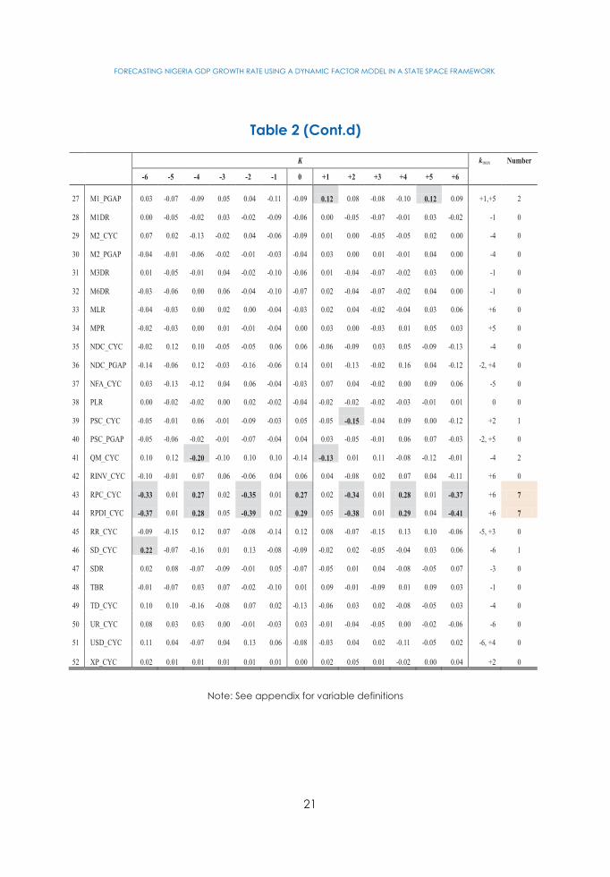
Table 2 (Cont.d)

K kmax Number

-6 -5 -4 -3 -2 -1 0 +1 +2 +3 +4 +5 +6

27 M1_PGAP

0.03

-0.07

-0.09

0.05

0.04

-0.11

-0.09

0.12

0.08

-0.08

-0.10

0.12

0.09

+1,+5

2

28 M1DR

0.00

-0.05

-0.02

0.03

-0.02

-0.09

-0.06

0.00

-0.05

-0.07

-0.01

0.03

-0.02

-1

0

29 M2_CYC

0.07

0.02

-0.13

-0.02

0.04

-0.06

-0.09

0.01

0.00

-0.05

-0.05

0.02

0.00

-4

0

30 M2_PGAP

-0.04

-0.01

-0.06

-0.02

-0.01

-0.03

-0.04

0.03

0.00

0.01

-0.01

0.04

0.00

-4

0

31 M3DR

0.01

-0.05

-0.01

0.04

-0.02

-0.10

-0.06

0.01

-0.04

-0.07

-0.02

0.03

0.00

-1

0

32 M6DR

-0.03

-0.06

0.00

0.06

-0.04

-0.10

-0.07

0.02

-0.04

-0.07

-0.02

0.04

0.00

-1

0

33 MLR

-0.04

-0.03

0.00

0.02

0.00

-0.04

-0.03

0.02

0.04

-0.02

-0.04

0.03

0.06

+6

0

34 MPR

-0.02

-0.03

0.00

0.01

-0.01

-0.04

0.00

0.03

0.00

-0.03

0.01

0.05

0.03

+5

0

35 NDC_CYC

-0.02

0.12

0.10

-0.05

-0.05

0.06

0.06

-0.06

-0.09

0.03

0.05

-0.09

-0.13

-4

0

36 NDC_PGAP

-0.14

-0.06

0.12

-0.03

-0.16

-0.06

0.14

0.01

-0.13

-0.02

0.16

0.04

-0.12

-2, +4

0

37 NFA_CYC

0.03

-0.13

-0.12

0.04

0.06

-0.04

-0.03

0.07

0.04

-0.02

0.00

0.09

0.06

-5

0

38 PLR

0.00

-0.02

-0.02

0.00

0.02

-0.02

-0.04

-0.02

-0.02

-0.02

-0.03

-0.01

0.01

0

0

39 PSC_CYC

-0.05

-0.01

0.06

-0.01

-0.09

-0.03

0.05

-0.05

-0.15

-0.04

0.09

0.00

-0.12

+2

1

40 PSC_PGAP

-0.05

-0.06

-0.02

-0.01

-0.07

-0.04

0.04

0.03

-0.05

-0.01

0.06

0.07

-0.03

-2, +5

0

41 QM_CYC

0.10

0.12

-0.20

-0.10

0.10

0.10

-0.14

-0.13

0.01

0.11

-0.08

-0.12

-0.01

-4

2

42 RINV_CYC

-0.10

-0.01

0.07

0.06

-0.06

0.04

0.06

0.04

-0.08

0.02

0.07

0.04

-0.11

+6

0

43 RPC_CYC

-0.33

0.01

0.27

0.02

-0.35

0.01

0.27

0.02

-0.34

0.01

0.28

0.01

-0.37

+6

7

44 RPDI_CYC

-0.37

0.01

0.28

0.05

-0.39

0.02

0.29

0.05

-0.38

0.01

0.29

0.04

-0.41

+6

7

45 RR_CYC

-0.09

-0.15

0.12

0.07

-0.08

-0.14

0.12

0.08

-0.07

-0.15

0.13

0.10

-0.06

-5, +3

0

46 SD_CYC

0.22

-0.07

-0.16

0.01

0.13

-0.08

-0.09

-0.02

0.02

-0.05

-0.04

0.03

0.06

-6

1

47 SDR

0.02

0.08

-0.07

-0.09

-0.01

0.05

-0.07

-0.05

0.01

0.04

-0.08

-0.05

0.07

-3

0

48 TBR

-0.01

-0.07

0.03

0.07

-0.02

-0.10

0.01

0.09

-0.01

-0.09

0.01

0.09

0.03

-1

0

49 TD_CYC

0.10

0.10

-0.16

-0.08

0.07

0.02

-0.13

-0.06

0.03

0.02

-0.08

-0.05

0.03

-4

0

50 UR_CYC

0.08

0.03

0.03

0.00

-0.01

-0.03

0.03

-0.01

-0.04

-0.05

0.00

-0.02

-0.06

-6

0

51 USD_CYC 0.11 0.04 -0.07 0.04 0.13 0.06 -0.08 -0.03 0.04 0.02 -0.11 -0.05 0.02 -6, +4 0

52 XP_CYC 0.02 0.01 0.01 0.01 0.01 0.01 0.00 0.02 0.05 0.01 -0.02 0.00 0.04 +2 0

Note: See appendix for variable definitions

21


4.2 Estimation Technique

4.2.1 Kalman Filtration

To provide forecasts for the real output growth, this study adopts

a dynamic factor model in a state space framework. The use of

the framework is motivated by its standard properties, namely,

that it allows for the incorporation of unobserved variables to be

estimated simultaneously with observed ones; and that it permits

the application of Kalman filtration in a recursive manner to

analyse the state space with capabilities for generating time-

varying parameters, missing data and effective handling of

measurement errors.

This provides a multivariate approach to the estimation of

unobservable variables by specifying them as function of the

observed variables in a state space framework. In this regard, the

procedure combines economic theory with time series tools,

allowing the unobservable variables to be interpretable. The

procedure for implementing Kalman filtration is usually recursive,

utilizing maximum likelihood techniques as shown in equations 4.1

and 4.2.

t ++t t t ty = Z â d í ()t tí ~ N 0, H

1 t+ ++t t t t tâ = Tâ c R ç ()t tç ~ N 0,Q

(1)

(2)

Equation 1 is the measurement, observation or signal equation,

while equation 2 is the state or transition equation. In the above

equations, , vector, , are the values of the observed time

series at a given time, . The irregular vector gives

observation disturbances, one for each of the time series in .

s

1p´ ty p

t 1p´ tí p

ty

22


The observation disturbances are assumed to have zero means

and positive definite unknown variance-covariance structure

given by the variance matrix is of order . The state

vector represents a set of unobserved variables and unknown

fixed effects, while the matrix of dimension links the

unobservable variables and regression effects of the state

vector with the observation vector . Matrix in equation 2 is the

transition matrix of dimension. The vector contains

the state disturbances with zero means and unknown variances

and covariances collected in the matrix of dimension . In

the above model, , an matrix, is included in front of the

state disturbance term in the model when is singular and

to make it work with nonsingular Durbin and Koopman, 2001;

Commandeur and Koopman, 2007; Mergner, 2009). However,

becomes an identity matrix where .

In the light of the above, algebraically, and can be shown to

be serially uncorrelated and normally distributed as follows:

tH p p 1m´

tâ

tZ p m

5 tT

m m 1r´ tç

tQ r r

tR m r

tQ r m<

tç

tR

r m=

5 The state vector has an initial state vector where is the mean vector

and the covariance matrices.

1m´ tâ ()~ N1 1 1â á ,P

1á

1P

tí

tç

(){

for t

otherwiseEt=

=tQ'

t ô 0ç ç

(){

for t

otherwiseEt

nn=

=tQ'

t ô 0

(3)

(4)

Also, the correlation between the state and observation

disturbances is assumed to be zero and independent of the

initial state vector , represented in algebraic terms as:

"

tâ

23


()E t ='

tç í 0 , 1, ,t Tt"=K,

(),E ='

t 1ç â 0 (),E ='

t 1í â 0 1, ,t T=K

(4.5)

(4.6)

It should be noted that the Kalman Filter estimation processes

can be optimal under the assumption of normally distributed

error schemes. Given that the conditional distributions of the

state vector are normal; their full specification is defined by the

first two moments which can be computed using Kalman filter

approach. Thus, the conditional mean, the first moment, is an

efficient estimator containing minimum MSE matrix. Mergner

(2009) show that even if the disturbances are not normal, “the

Kalman filter is no longer guaranteed to yield the conditional

mean of the state vector.Thus, the Kalman filter can still be

applied if the normality assumption is relaxed.

In the light of the above, the empirical dynamic factor model for

forecasting GDP is specified to include six measurement

equations and two state equations. The included variables are

obtained through the examination of the strength of the

dynamic cor re lat ion between growth and other

macroeconomic indicators. The exercise identifies factors with

strong co-movement and the possibility of having common

factors with growth. This obviously strengthens forecast

performance and provides insight on the growth path from

available high frequency macroeconomic time series variables.

4.2.2 Growth Dynamic Factor Model

6

6 In the literature estimators that are derived through the maximization of the Gaussian likelihood function with non-normal observations are called quasi-maximum likelihood (QML) estimators (see Hamilton, 1994; Mergner, 2009).

24


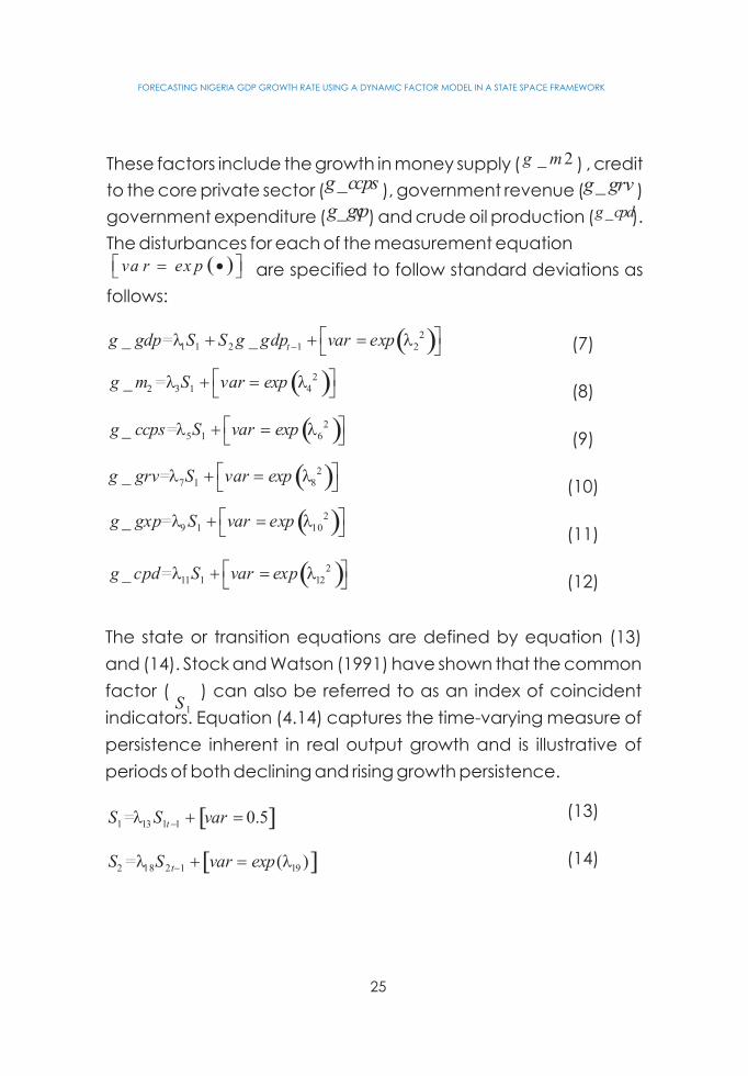
These factors include the growth in money supply ( ) , credit

to the core private sector ( ), government revenue ( )

government expenditure ( ) and crude oil production ( ).

The disturbances for each of the measurement equation

are specified to follow standard deviations as

follows:

_ 2g m

_g ccps _g grv

_g gxp _g cpd

()va r ex pé ù=·ë û

()21 1 2 1 2=_ _ tg gdp S S g gdp var expl l-é ù+ +=ë û

()22 3 1 4=_g m S var expl lé ù+=

ë û

()25 1 6=_g ccps S var expl lé ù+=

ë û

()27 1 8_ =g grv S var expl lé ù+=ë û

()29 1 10_ =g gxp S var expl lé ù+=ë û

()211 1 12=_g cpd S var expl lé ù+=

ë û

(7)

(8)

(9)

(10)

(11)

(12)

The state or transition equations are defined by equation (13)

and (14). Stock and Watson (1991) have shown that the common

factor ( ) can also be referred to as an index of coincident

indicators. Equation (4.14) captures the time-varying measure of

persistence inherent in real output growth and is illustrative of

periods of both declining and rising growth persistence.

1S

[ ]1 13 1 1= 0.5tS S varl-+=

[ ]2 18 2 1 19( )= tS S var expl l-+=

(13)

(14)

25


4.2.3 Forecasting Growth

In order to forecast the real output growth, the forecast of ( )

from the above dynamic factor model is generated over the

extended horizon. This is then multiplied by the estimate of

lambda obtained from equation (7) for each period

over the forecast horizon. Thereafter, the mean of the rate of

growth of GDP is added to these products recalling that the

above model is estimated after the included observation

variables were demeaned.

tS

_i g gd pl

26


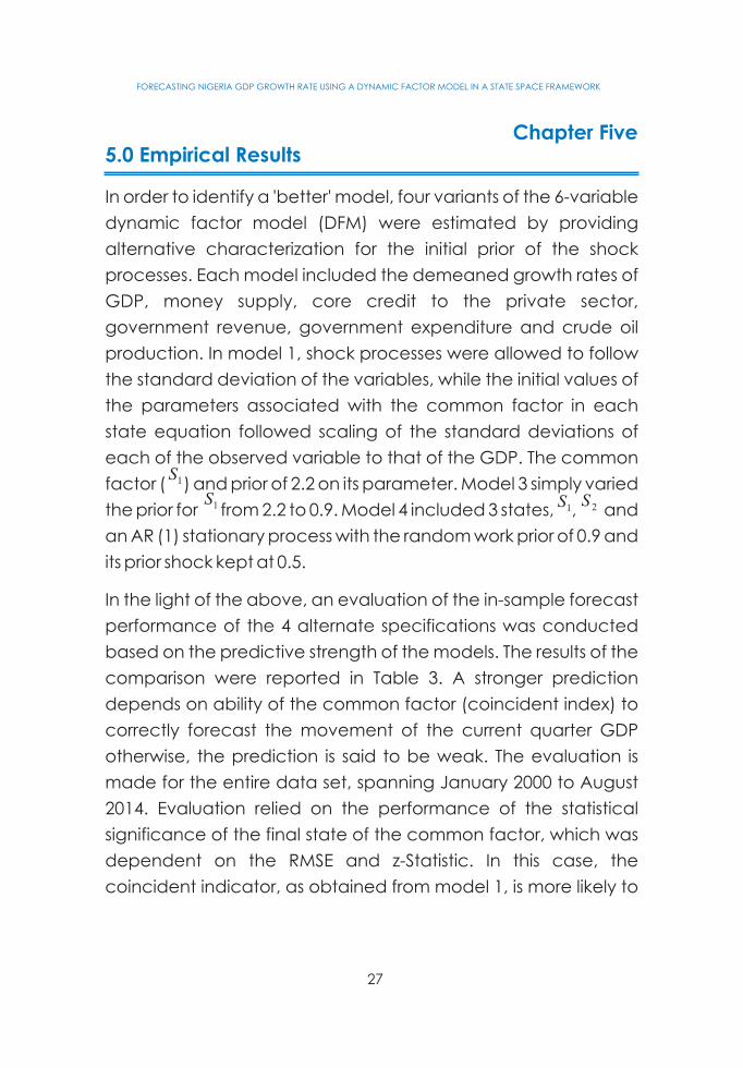
In order to identify a 'better' model, four variants of the 6-variable

dynamic factor model (DFM) were estimated by providing

alternative characterization for the initial prior of the shock

processes. Each model included the demeaned growth rates of

GDP, money supply, core credit to the private sector,

government revenue, government expenditure and crude oil

production. In model 1, shock processes were allowed to follow

the standard deviation of the variables, while the initial values of

the parameters associated with the common factor in each

state equation followed scaling of the standard deviations of

each of the observed variable to that of the GDP. The common

factor ( ) and prior of 2.2 on its parameter. Model 3 simply varied

the prior for from 2.2 to 0.9. Model 4 included 3 states, , and

an AR (1) stationary process with the random work prior of 0.9 and

its prior shock kept at 0.5.

In the light of the above, an evaluation of the in-sample forecast

performance of the 4 alternate specifications was conducted

based on the predictive strength of the models. The results of the

comparison were reported in Table 3. A stronger prediction

depends on ability of the common factor (coincident index) to

correctly forecast the movement of the current quarter GDP

otherwise, the prediction is said to be weak. The evaluation is

made for the entire data set, spanning January 2000 to August

2014. Evaluation relied on the performance of the statistical

significance of the final state of the common factor, which was

dependent on the RMSE and z-Statistic. In this case, the

coincident indicator, as obtained from model 1, is more likely to

1S

1S

1S 2S

27

Chapter Five5.0 Empirical Results


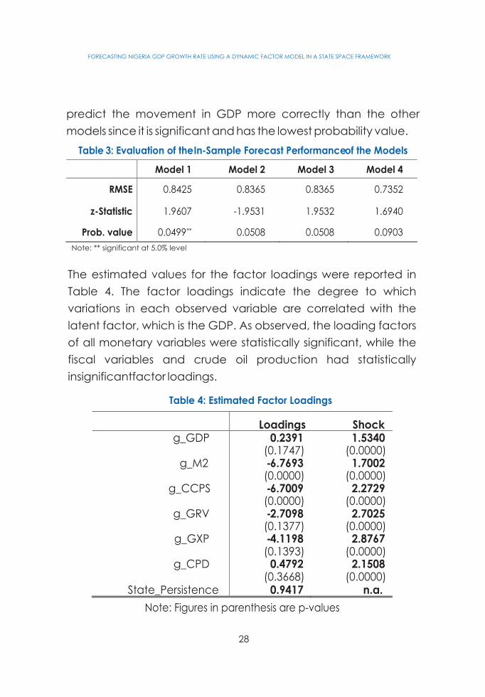
Table 3: Evaluation of the In-Sample Forecast Performance

of the Models

Model 1

Model 2

Model 3

Model 4

RMSE 0.8425 0.8365 0.8365 0.7352

z-Statistic 1.9607 -1.9531 1.9532 1.6940

Prob. value

0.0499**

0.0508

0.0508

0.0903

Note: ** significant at 5.0% level

The estimated values for the factor loadings were reported in

Table 4. The factor loadings indicate the degree to which

variations in each observed variable are correlated with the

latent factor, which is the GDP. As observed, the loading factors

of all monetary variables were statistically significant, while the

fiscal variables and crude oil production had statistically

insignificantfactor loadings.

Table 4 : Estimated Factor Loadings

Loadings Shockg_GDP 0.2391 1.5340

(0.1747) (0.0000)g_M2 -6.7693 1.7002

(0.0000) (0.0000)g_CCPS

-6.7009

2.2729

(0.0000)

(0.0000)g_GRV

-2.7098

2.7025

(0.1377)

(0.0000)g_GXP

-4.1198

2.8767(0.1393)

(0.0000)g_CPD

0.4792

2.1508(0.3668)

(0.0000)State_Persistence 0.9417 n.a.

Note: Figures in parenthesis are p-values

28


predict the movement in GDP more correctly than the other

models since it is significant and has the lowest probability value.

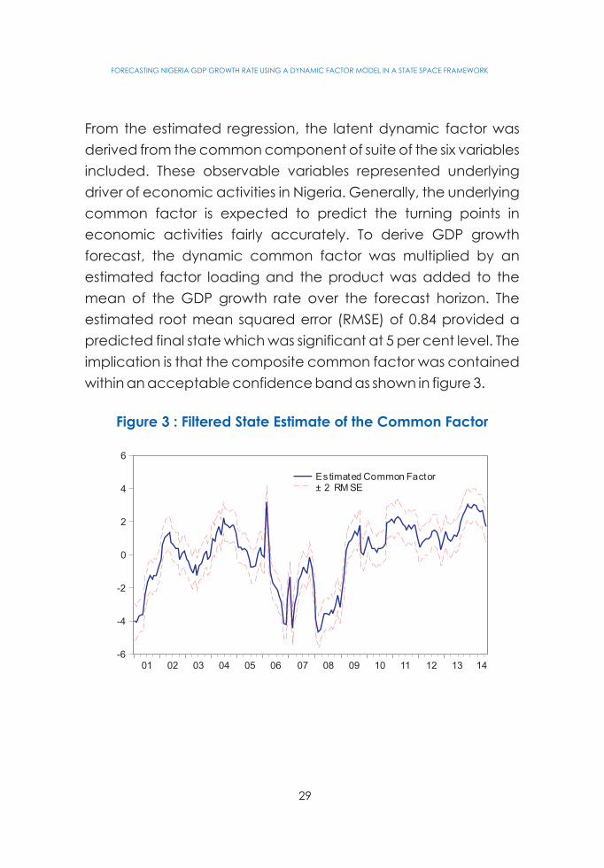
From the estimated regression, the latent dynamic factor was

derived from the common component of suite of the six variables

included. These observable variables represented underlying

driver of economic activities in Nigeria. Generally, the underlying

common factor is expected to predict the turning points in

economic activities fairly accurately. To derive GDP growth

forecast, the dynamic common factor was multiplied by an

estimated factor loading and the product was added to the

mean of the GDP growth rate over the forecast horizon. The

estimated root mean squared error (RMSE) of 0.84 provided a

predicted final state which was significant at 5 per cent level. The

implication is that the composite common factor was contained

within an acceptable confidence band as shown in figure 3.

Figure 3 : Filtered State Estimate of the Common Factor

-6

-4

-2

0

2

4

6

01 02 03 04 05 06 07 08 09 10 11 12 13 14

Estimated Common Factor± 2 RM SE

29


The plot of the unobserved common factor of the included

variables exhibited three prominent phases (2001-2006), (2006-

2009) and (2009-2014). While the first phase showed a rise with

twin spikes in 2002 and 2004, the second phase witnessed

moderate declines. The upward beat was resumed in the last

sub-sample and that was sustained from 2009 through 2014. A rise

(or a fall) in the underlying factor suggested a rise (or a fall) in the

GDP rate, depending on the sign (positive or negative) of the

loading factors.

The estimated common component, the underlying factor,

contained vital information for forecasting economic growth in

Nigeria. Many authors including Schulz (2008), Forni et al. (2000),

Stock and Watson (2002) and Banerjee et al. (2006) recognised

the significance of common components as leading factors for

forecasting economic activities. Schulz (2008) using a composite

lead derived from dynamic principal component analysis to

forecast economic growth for Estonia. In this study, the common

factor is derived directly from a dynamic state space

specification as the composite lead for GDP growth in a data set

that also included money supply, credit to core private sector,

government revenue, government expenditure, and Nigeria's

crude oil production. The importance of composite lead is not

only in forecasting accurate GDP growth numbers, but in its

ability to predict turning points which is of considerable value to

policymakers (Chin et al., 2000). Figure 4 juxtaposed the

estimated dynamic common factor – composite leading

indicator – with real GDP growth in Nigeria. It showed a common

5.1 Forecasting the GDP Growth: the Estimated Common

Component

30


long-run trend between the underlying factor and the economic

growth.

Apart from the outliner growth periods in 2004, the chart depicted

some congruence in between the indictor and the reference

series. This however, contained phase shifts in the ability of the

composite leading indicator to track turning points in real GDP

growth. A fall in the reference series is preceded by a decline in

the composite leading indicator, and vice versa for a rise.

However, the number of lags (i.e. delay) between the turning

points in the indicator and reference series seem to be reducing.

This phase shifts suggest improving track-ability of the composite

leading indicator.

Figure 4 : Composite Leading Indicator and GDP Growth

-8

-4

0

4

8

12

16

20

01 02 03 04 05 06 07 08 09 10 11 12 13 14

ORIG_G_GDPS1

31


As shown in the chart, the peaks and trough observed in the real

GDP growth around 2007 and 2008 were reliably predicted by

composite leading indicator with a delay of nearly 2 years. By

2010, the delay could be seen to have shortened to just over 4

quarters. Towards the end of the plots, the graph indicated that,

more recently, delay in predicting the turning points have been

reduced to about 3 quarters. Hence, the slightly southward

orientation of the composite leading indicator observable

towards the end of the series could suggest some deceleration

of economic activities by the middle of 2015. This is indeed not

inexplicable. The chart showed a plunge in observed real GDP

growth rates in the periods after general elections in 2003, 2007,

and 2011.

Applying the estimated loading factor for the reference series to

the composite leading indicator, and adjusting for the mean,

real GDP growth forecasts were derived for the period 2014:Q3

to 2105:Q4. As noted earlier, a RMSE analysis selected the

originating state space specification as the best model among

alternative specifications. The actual and forecast growth rates

were plotted in Figure 2. The forecast showed a robust real GDP

growth rate which generally remained above 6.50 per cent.

Output acceleration was forecasted for 2014:Q3, with growth

rate predicted to rise from 6.54 per cent in 2014:Q2 to 6.93 per

cent. Nonetheless, a modest slowdown is predicted towards the

end of 2014 and throughout 2015. Based on the composite

leading indicator, GDP growth rates for 2015:Q2 and 2015:Q4

were forecasted as 6.83 per cent and 6.75 per cent, respectively,

indicative of a slowdown.

32


Figure 5 : GDP Growth Rate - Actual and Forecast (%)

5.5

6.0

6.5

7.0

7.5

8.0

I II III IV I II III IV I II III IV I II III IV

2012 2013 2014 2015

forecast

33


The need for a more consistent and accurate GDP forecast for

the conduct of forward-looking monetary policy is quite

fundamental. This is because the availability of real-time data is

crucial to determine the initial conditions of economic activity on

latent variables such as the output gap to make policy decisions.

The study developed a framework that enables the forecasting of

quarterly GDP growth for Nigeria using a dynamic factor model in

a state space methodology. This approach is anchored on its

ability to extract underlining factors among a set of

macroeconomic variables that contain information about the

latent state of the economy that can be used in generating

robust and reliable GDP forecast. The DFM provide help to

addressing the paucity of real-time data. It also permits the

utilisation of a mixture of data frequencies in the determination of

the current state of the economy.

Prior to estimation, the dynamic correlations between the GDP

growth rates and fifty-two (52) macroeconomic variables were

constructed. This helps in the identification of the best six leading

indicators of economic/growth cycles namely; that government

revenue, government expenditure, crude oil production and

core credit to the private sector. Efforts were also made to

characterise this growth cycles for enhanced understanding of

the boom and bust sessions associated with business cycles in

economic literature. The underlying common factor mimics the

turning points in growth trajectory relatively well. It signals three

distinct regimes that align with the direction of the movement of

GDP growth rate based on the loading factors.

34

Chapter Six6.0 Conclusion


The study revealed that of the four variants of the model

investigated, model one (1) appeared to be the most preferred,

as it predicted the movement in real GDP growth rate more

accurately than the other models. The model showed robust real

GDP growth forecasts of 6.54, 6.93, 6.83 and 6.75 per cent in

2014Q3, 2014Q4, 2015Q2 and 2015Q4, respectively. The model

did not only assist in computing a coincident lead indicator for

Nigeria, but also explained a very high percentage of the

variance of actual GDP growth rate. The model is, thus, a valid

tool for tracking the business cycle.

35


Allen D. S. and M. Pasupathy (1997).“A State Space Forecasting

Model with Fiscal and Monetary Control”, Federal Reserve

Bank of St. Louis Working Paper No. 017A.Anderson R. G. and C. S. Gascon (2009). “Estimating U.S. Output

Growth with Vintage Data in a State-Space Framework', Federal Reserve Bank of St. Louis Review, July/August, 91(4), pp. 349-69.

Banerjee A., M. Marcellino, I. Masten (2006). “Forecasting Macroeconomic Variables for the New Member States,” In Artis, M., A. Banerjee, and M. Marcellino (Eds.), Central and Eastern European Countries and the European Union, Cambridge: Cambridge University Press.

Beak M. (2010). “Forecasting Hourly Electricity Loads of S o u t h K o r e a : I n n o v a t i o n s S t a t e S p a c e ModelingApproach,” The Korean Journal of Economics Vol. 17, No. 2(Autumn 2010).

Beòkovskis K. (2008).” Short-Term Forecastsof Latvia's Real Gross Domestic Product Growthusing Monthly Indicators”, Latvijas Bank Working Paper, No 5.

Box, G. E. P. and G.M. Jenkins (1976).“Time Series Analysis”, Forecasting and Control, San Francisco CA, Holden Day.

Branimir, J. and P. Magdalena, (2010). “Forecasting Macedonian GDP: Evaluation of different models for short-term forecasting”, Personal RePEc Archive, WP/43162.

Camacho M., M. Dal Bianco and J. Martínez-Martín (2013)”, Short-Run Forecasting of Argentine GDP Growth”, BBVA Working PaperNumber 13/14.

Chin D., J. Geweke, and P. Miller (2000).“Predicting Turning Points”, Technical Paper Series, Congressional Budget Office.

Clarida R, J. Gali, M. Gertler (2000). “Monetary Policy Rules and

Macroeconomic Stability: Evidence and Some Theory”,

Quarterly Journal of Economics, 115(1):147-180.

Munich

36


Reference

Commandeur, Jacques J. F. and Siem J. Koopman (2007).

Practical Econometrics: an introduction to State Space

Time Series Analysis. Oxford, UK: Oxford University Press.

Doz C.,D.Giannone and L. Reichlin (2006)."A quasi maximum

likelihood approach for largeapproximate dynamic factor

models".CEPR Discussion Paper No. 5724.

Doz C., D.Giannone and L.Reichlin (2007)."A two-step estimator

for large approximate dynamic factor models based on

Kalman filtering".CEPR Discussion Paper No 6043.

Durbin, J. and S. J. Koopman (1997). Monte Carlo maximum

likelihood estimation for non-Gaussian state space

models”.Biometrika 84(3), 669 – 684.

Ehrmann, M and F. Smets (2003). “Uncertain Potential Output:

Implications for Monetary Policy”, Journal of Economic

Dynamics and Control,27, 1611-1638.

Fenz, G. and M. Spitzer (2005).“An Unobserved Components

Model to forecast Austrian GDP”, Oesterreichische

Nationalbank, Working Paper 119.

Fenz,G., M. Schneider and M. Spitzer (2004). Macroeconomic

Models and Forecasts for Austria” Proceedings of

Oesterreichische Nationalbank (OeNB) Workshops No.

5/2005

Forni M., M. Hallin, M. Lippi and L. Reichlin (2000).“The Generalized

Factor Model: Identification and Estimation”, The Review of

Economics and Statistics, No.82, pp 540–54.

Forni, M., M. Hillini, M. Lippi and L. Reichlin (2004). “The Generalized

Dynamic factor model: consistency and rates”, Journal of

Econometrics 119,231-255.

Hamilton J.D. (1989).“A New Approach to the Economic Analysis

of Nonstationary Time Series and the Business Cycle”,

Econometrica, No.57, pp.357–84

Hamilton, J. D. (1994). State-space Models. In R.F. Engle and D.L.

McFadden (Eds), Handbook of Econometrics, Volume 4,

37


Chapter 50, 3039-3080. Amsterdam, The Netherlands:

Elsevier Science B.V.

Hindrayanto I., S. J. Koopman and J. Winter (2014).”Nowcasting

and Forecasting EconomicGrowth in the Euro Area using

PrincipalComponents”, Tinbergen Institute Discussion

Paper No. TI 2014-113/III

Jonanovic, B. and M. Petrovska (2010). “Forecasting

Macedonian GDP: Evaluation of Different Models for Short-

Term Forecasting”, National Bank of the Republic of

Macedonia, Working Paper, August.

Kozicki S. (2004). “How Do Data Revisions AffectThe Evaluation

and Conduct ofMonetary Policy?”, Federal Reserve Bank

of Kansas City Economic Review, First Quarter.

Kugler, P., T. J. Jordan, C. Lenz and M. R. Savioz (2004).

“Measurement Errors in GDP and Forward-looking

Monetary Policy: The Swiss Case”, Deutsche Bundesbank,

Discussion Paper Series 1: Studies of the Economic

Research Centre No 31.

Litterman R. B. (1986). ”Forecasting with Bayesian Vector

Autoregressions-Five years of experience”, Journal of

Business and Economic Statistics, Vol.4, pp.25-38.

Mergner, Sascha (2009). Applications of State Space Models in

Finance: An Empirical Analysis of the Time-varying

Relationship between Macroeconomics, Fundamentals

and Pan-European Industry Portfolios. Universitätsverlag

Göttingen http://univerlag.uni-goettingen.de

Nadal-De Simone F. (2000). “Forecasting Inflation in Chile using

State-Space and Regime-Switching Models”, IMF Working

Paper. WP/001/162.

Orphanides, A. (2000) “The Quest for Prosperity Without

Inflation”, European Central Bank Working Paper No. 15.

Orphanides, A. (2001) “Monetary Policy Rules Based on Real-

Time Data”, American Economic Review, 91, 964-985.

38


Schulz C. (2007).”Forecasting Economic Growth for Estonia:

Application of Common Factor Methodologies”, Bank of

Estonia Working Paper Series No 9

Schulz C. (2008). “Forecasting Economic Activity for Estonia: The

Application of Dynamic Principal Components Analysis”,

Bank of Estonia Working Paper Series 2/2008.

Schumacher, C. and C. Dreger (2005).“Estimating large scale

factor models for economic activity in Germany: Do they

outperform simpler models?”, Jahrbbiucher fur

Nationalokonomie und Statistik 224, 731-750.

Sims, C. A. (1993). “A Nine Variable Probabilistic Macroeconomic

Forecasting Model”, in NBER Studies in Business: Business

Cycles, Indicators, and Forecasting, Volume 28. James H.

Stock and Mark W. Watson, eds. Chicago: University of

Chicago Press, pp. 179–214.

Sims, C. A. and T.Zha (1996)."Bayesian methods for dynamic

multivariate models", Federal Reserve Bank of Atlanta

Working Paper 96-13.

Stock J.H. and M.W. Watson (2002).“Forecasting Using Principal

Components from a Large Number of Predictors”, Journal

of the American Statistical Association, No.97, pp 147–62

Stock, J.H. and M.W. Watson (1991). A probability model of the

coincident economic indicators. In K. Lahiri and G.H.

Moore (Eds.), Leading Economic Indicators: New

Approaches and Forecasting Records, 63-89. Cambridge,

UK: Cambridge University Press.

Stock, J. H., and M. Watson (1989). “New Indexes of Coincident

and Leading Economic Indicators., in O. Blanchard and S.

Fischer (Eds.), NBER Macroeconomics Annual, Vol. 4, pp.

351-409.

39


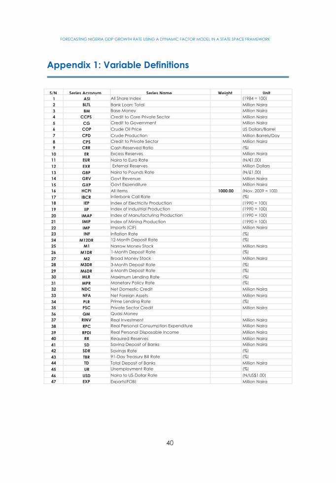
Appendix 1: Variable Definitions

S/N Series Acronym Series Name Weight Unit

1 ASI All Share Index (1984 = 100)

2 BLTL Bank Loan: Total Million Naira

3 BM Base Money Million Naira

4 CCPS Credit to Core Private Sector Million Naira

5 CG Credit to Government Million Naira

6 COP Crude Oil Price US Dollars/Barrel

7 CPD Crude Production Million Barrels/Day

8 CPS Credit to Private Sector Million Naira

9 CRR Cash Reserved Ratio (%)

10 ER Excess Reserves Million Naira

11 EUR Naira to Euro Rate (N/€1.00)

12 EXR External Reserves Million Dollars

13 GBP Naira to Pounds Rate (N/£1.00)

14 GRV Govt Revenue Million Naira

15 GXP Govt Expenditure Million Naira

16 HCPI All Items 1000.00 (Nov. 2009 = 100)

17 IBCR Interbank Call Rate (%)

18 IEP Index of Electricity Production (1990 = 100)

19 IIP Index of Industrial Production (1990 = 100)

20 IMAP Index of Manufacturing Production (1990 = 100)

21 IMIP Index of Mining Production (1990 = 100)

22 IMP Imports (CIF) Million Naira

23 INF Inflation Rate (%)

24 M12DR 12-Month Deposit Rate (%)

25 M1 Narrow Money Stock Million Naira


27 M2 Broad Money Stock Million Naira



30 MLR Maximum Lending Rate (%)

31 MPR Monetary Policy Rate (%)

32 NDC Net Domestic Credit Million Naira

33 NFA Net Foreign Assets Million Naira

34 PLR Prime Lending Rate (%)

35 PSC Private Sector Credit Million Naira

36 QM Quasi Money

37 RINV Real Investment Million Naira

38 RPC Real Personal Consumption Expenditure Million Naira

39 RPDI Real Personal Disposable Income Million Naira

40 RR Required Reserves Million Naira

41 SD Saving Deposit of Banks Million Naira

42 SDR Savings Rate (%)

43 TBR 91-Day Treasury Bill Rate (%)

44 TD Total Deposit of Banks Million Naira

45 UR Unemployment Rate (%)

46 USD Naira to US-Dollar Rate (N/US$1.00)

47 EXP Exports(FOB) Million Naira


40

Appendix 2: The Markov Chain Model

GDP growth rate is modelled to be characterised by two states:

high and low growth periods. The high state represents periods of

rising growth rate (output acceleration) and the low state reflects

a regime of declining growth rate (output slowdown). A 2-regime

multivariate Markov Chain model is, thus, fitted where GDP

growth is allowed to follow an AR(1) process specified as:

(3.1)

where is the vector of exogenised drivers of the growth

cycle. As defined by Hamilton (1989) the transition probabilities

reflects the switch from regime 2 to regime

1, and is the probability of switching from

regime 1 to regime 2. The associated transition matrix is defined

as

æ ö=ç ÷è ø

11 12

21 22

p p

p pM (3.2)

where the conditions and are satisfied to ensure

that the estimated probabilities are irreducible in the 2 states

while the ergodic condition are also expected to

hold. Hence, and is generally satisfied.


41

CENTRAL BANK OF NIGERIA

ISBN - 978-978-951-926-2

forecasting nigeria gdp growth rate using a dynamic factor ... forecasting gdp.pdf · common factor...

Documents