Working Paper/Document de travail 2012-37

Forecasting Inflation and the Inflation Risk Premiums Using Nominal Yields

by Bruno Feunou and Jean-Sébastien Fontaine

2

Bank of Canada Working Paper 2012-37

November 2012

Forecasting Inflation and the Inflation Risk Premiums Using Nominal Yields

by

Bruno Feunou and Jean-Sébastien Fontaine

Financial Markets Department Bank of Canada

Ottawa, Ontario, Canada K1A 0G9 jsfontaine@bankofcanada.ca

Bank of Canada working papers are theoretical or empirical works-in-progress on subjects in economics and finance. The views expressed in this paper are those of the authors.

No responsibility for them should be attributed to the Bank of Canada.

ISSN 1701-9397 © 2012 Bank of Canada

ii

Acknowledgements

We thank Antonio Diez, Scott Hendry, Sharon Kozicki, Philippe Mueller and Norm Swanson for comments and suggestions. We thank Timothy Grieder for research assistance.

iii

Abstract

We provide a decomposition of nominal yields into real yields, expectations of future inflation and inflation risk premiums when real bonds or inflation swaps are unavailable or unreliable due to their relative illiquidity. We combine nominal yields with surveys of inflation forecasts within a no-arbitrage model where conditional expectations are latent but spanned by the history of the observed data, analog to a GARCH model for the conditional variance. The filtering problem is numerically trivial and we conduct a battery of out-of-sample comparisons. Our favored model matches the quarterly inflation forecasts from surveys and uses the information in yields to produce the best monthly forecasts. Moreover, we restrict the distribution of the inflation Sharpe ratios to achieve economically reasonable estimates of the inflation risk premium and of the real rates. We find that the inflation risk premium (i) is positive on average, (ii) rises when the unemployment rate increases and (iii) when the level of interest rates decreases. Hence, real yields are more pro-cyclical than nominal yields due to variations of the inflation risk premiums.

JEL classification: E43, E47, G12 Bank classification: Asset pricing; Econometric and statistical methods; Interest rates; Inflation and prices

Résumé

Les auteurs proposent de décomposer les taux de rendement nominaux en trois éléments – taux réels, inflation anticipée et primes de risque d’inflation – lorsqu’il n’existe pas d’obligations ou de swaps indexés sur l’inflation ou que les données ne sont pas fiables en raison de l’illiquidité relative de ces instruments. Ils combinent les prévisions d’inflation recueillies par enquête aux rendements nominaux dans le cadre d’un modèle fondé sur l’absence d’arbitrage où les anticipations conditionnelles sont latentes mais dépendent des observations passées, à la manière de la variance conditionnelle dans un modèle GARCH. Le problème de filtrage est simple numériquement, ce qui permet aux auteurs de comparer entre elles un grand nombre de prévisions hors échantillon. Leur modèle parvient à reproduire les prévisions d’inflation trimestrielles tirées d’enquêtes, et c’est aussi celui qui fournit les meilleures prévisions mensuelles grâce à l’information extraite des taux nominaux. Les auteurs imposent en outre des restrictions à la distribution des ratios de Sharpe associés au risque d’inflation pour obtenir des estimations économiquement raisonnables de la prime de risque d’inflation et des taux réels. Ils constatent que la prime est positive en moyenne et qu’elle s’accroît quand le taux de chômage monte ou que les taux d’intérêt baissent. La procyclicité des rendements réels serait ainsi plus marquée que celle des rendements nominaux à cause de la variation des primes de risque d’inflation.

Classification JEL : E43, E47, G12 Classification de la Banque : Évaluation des actifs; Méthodes économétriques et statistiques; Taux d’intérêt; Inflation et prix

Introduction

The decomposition of market interest rates into a component attributable to the effect of

inflation and a component attributable to real effects has a long history. Irving Fisher was

prominent among classical economists in this regards (Fisher, 1930) and the well-known

decomposition of nominal yields into real yields and compensation for inflation bears his

name. In the absence of risk, the real yield can be obtained by subtracting a measure of

expected inflation ‘from the nominal yield. But this simplicity hides the fact that future

inflation rates are difficult to forecast (see e.g. Stock and Watson 2007). Furthermore, risk

adds considerable difficulty to the decomposition since the unobserved inflation risk premium

contributes significant variations to nominal yields (Buraschi and Jiltsov, 2005).

The recent literature uses separate measurements for each element of Fisher’s decomposi-

tion. Chernov and Mueller (2011) combine nominal yields, surveys of inflation forecasts and

data from inflation-indexed bond. Similarly, Haubrich, Pennacchi, and Ritchken (2012) use

nominal yields, surveys of inflation forecasts and inflation swap data (instead of real bonds).

But these additional instruments are not available in many countries, at least not for the

horizons of interest. Moreover, using real bond or inflation swap data relies on additional

maintained hypotheses about the degree of integration between different markets and about

the magnitude and variations of any liquidity premium. These assumptions may not be sup-

ported in the data (Campbell, Shiller, and Viceira 2009, Fleckenstein, Longstaff, and Lustig

2012, Pflueger and Viceira 2011, Christensen and Gillan 2011). Our main contribution is

to provide an accurate decomposition of the nominal yield curve that does not rely on the

availability (or reliability) of real bonds or inflation swaps. Empirically, we consider the case

of Canadian interest rates but our approach has broad applicability.1

Our approach relies on three distinct but complementary ingredients. First, we provide a

careful and parsimonious specification for the evolution of expected inflation. As Kim (2007)

pointed out, inflation expectations are persistent but the inflation shocks are large and mostly

transitory, something that is hard to capture within a standard macro-finance VAR(1) model.

One common solution is to introduce a latent factor to represent expectations directly. But

the associated filtering problem carries its own challenges. We depart from this common

approach and represent the evolution of inflation and other macro and finance variables

via a conditional mean model (Fiorentini and Sentana, 1998) where expected inflation is

1Inflation swap data are not available in Canada. Moreover, existing real bonds have very long maturitiesand carry a time-varying liquidity premium. The shortest maturity of real returns bonds in Canada isDecember 2021, making these instruments inappropriate to construct short- to medium- inflation forecastsin our sample.

persistent but where the effect of inflation innovations is transitory.2 Instead of being purely

latent, unobserved expected inflation is spanned by the history of the other state variables.

The filtering problem becomes trivial and we can easily assess the inflation forecasts from

the model in a wide range of out-of-sample exercises.

Second, the conditional mean specification leads to a (discrete-time) affine dynamic term

structure model. We develop two types of economic restrictions on the prices of risk to

achieve an accurate and sensible measure of the inflation risk premium. In the spirit of Duffee

(2011), we constrain the inflation Sharpe ratio.3 Specifically, we restrict the parameter space

so that the conditional inflation Sharpe ratio lies within the interval [−SR, SR] with 95%

probability in population. This restriction is similar but simpler than the approach taken

by Duffee (2011).4 In practice, we consider a range of values for SR. Our second restriction

follows Chernov and Mueller (2011) and imposes that the short real rate and the real yields

are not functions of inflation expectations contemporaneously. We show that this implies

a connection between, on one hand, the response of the nominal short rate to expected

inflation and, on the other hand, the response of the inflation risk premium to expected

inflation. Therefore, restrictions on the Sharpe ratio advocated by Duffee (2011) affect

estimate of the inflation coefficient in the nominal rate when combined with the exclusion

of inflation from the real rate advocated by Chernov and Mueller (2011). The interaction

between these two restrictions implies that imposing a very low or zero one-period inflation

Sharpe ratio to obtain accurate measures of the real yields (as in Ang, Bekaert, and Wei

2008) leads to unreasonable estimates of the policy response to expected inflation.

Third, we add survey data at estimation to counter the loss in parsimony.5 Formally, we

rely on the additional assumption that survey forecasts are rational, implying that they are

consistent with model inflation forecasts up to an unpredictable error term. Estimation is

then based on the combination of the likelihood of survey observations with the likelihood

of the model. Survey data is available for most developed countries but, on the other hand,

at a frequency that is often too slow or irregular, leading to a missing variable problem for

many of the existing models. This poses no difficulties in our model given the simplicity of

the filter.

Empirically, we estimate a conditional mean specification where the state variables are

2Our specification has a VARMA representation of order (1,1).3Joslin et al. (2011) discuss the role of economic restrictions in the estimation of term structure models.

See also Bauer and Diez (2012) in the context of a multi-country term structure model.4Duffee (2010) numerically penalizes Sharpe ratio realizations that are too high point by point within the

estimation procedure.5Kim and Orphanides (2012) discuss extensively the use of survey of yield forecasts to reduce sampling

uncertainty and lessen the bias in estimates of persistence parameters.

2

the inflation rate, the unemployment rate and two term structure factors. We use data on

nominal yields and survey forecasts from 1986 until 2012. Following a battery of out-of-

sample forecasting exercises, we conclude that the combination of (i) a conditional mean

model, (ii) estimation based on survey data, and (iii) the information content of yields

produces the best out-of-sample inflation forecasts. A conditional mean model outperforms

simpler VARs across a range of univariate, bivariate or multivariate specifications. Neglecting

surveys affects forecast accuracy even if surveys are available only infrequently and for a

subset of horizons.6 Innovations in the level and slope of the term structure have a persistent

effect on expected inflation but inflation innovations do not.7

Having established the accuracy of the inflation forecasts, we turn to our estimates of

real yields and of inflation risk premiums. We find that the inflation risk premium increases

when the unemployment rate increases and when the level of yields is low. This is consistent

with risk aversion being higher in recession: losses due to unexpected inflation shocks carry

a greater weight in those states. Alternatively, the response of the central bank to infla-

tion shocks may have more adverse consequences when the unemployment rate is higher.

The results imply that real yields are negatively correlated with the inflation risk premium

throughout the cycle. Moreover, estimates of real yields that account for the inflation risk

premium are lower than unadjusted estimates in recessionary or low-growth episodes. In

other words, real yields appear more pro-cyclical than nominal yields once we adjust for the

inflation risk premium.

Pennacchi (1991) and Ang, Bekaert, and Wei (2008) also combines economic restrictions

and nominal yields within dynamic term structure models. Pennacchi (1991) considers an

equilibrium model and uses surveys to pin down the evolution of expectations but he does

not measure the inflation risk premium. Ang, Bekaert, and Wei (2008) consider an affine

no-arbitrage model with regimes. They impose a zero one-period inflation risk premium to

identify the level of real rates. Regime-switching models are difficult to implement and to

interpret. Moreover, the zero premium assumption has far-reaching consequences on the

inflation Sharpe ratios, on the variability of the inflation risk premium (across different

horizons) and on the estimates of the policy response coefficients. More recently, Chun

6This result echoes results in Faust and Wright (2011) for the case of the US. Several models matchsurvey accuracy at the quarterly frequency where surveys are available. This contrasts with results in Anget al. (2007) for the US who find that survey forecasts are difficult to match but they do not use survey atestimation.

7In their review of the literature, Stock and Watson (2003) find no evidence that nominal yields containmarginal information for future inflation. They argue that this reflects “limitations of conventional model[...], not a fundamental absence of predictive relationships in the economy.” Stock and Watson (2003),p.79. We find that combining survey data with yield data in a sufficiently rich model delivers significantpredictability.

3

(2011) uses US survey and yield data in combination with a term-structure model but do

not decompose yields. Ajello, Benzoni, and Chyruk (2012) combine measures of core, food,

and energy inflation series and obtain a decomposition of yield within a term structure

model. Most of these studies do not assess the inflation expectations (via out-of-sample

forecast comparison) or do not constrain the inflation risk premium around economically

reasonable values.8 Kozicki and Tinsley (2001) and Kozicki and Tinsley (2006) explores the

role of shifting end-points in the processes for long-horizon yields or inflation rates in the

US. In Canada, Amano and Murchison (2006) show the importance of a shifting endpoint

for inflation in the early 1990s during the transition toward a 2% inflation targeting regime.

Ragan (1995) is an early attempt to measure anticipation of future inflation from nominal

yields in Canada. However, he assumes a constant risk premium. Day and Lange (1997)

provides time-series evidence that the term spread has predictive content for inflation rates

over the medium-term. Fung, Mittnick, and Remolona (1999) study a joint model for the US

and Canadian term structure and identify the inflation factor by assuming that it is specific

to each country while the real factor is common to both countries. They do not use survey

data to identify inflation expectations. Garcia and Luger (2007) estimate an equilibrium-

based model where investors derive utility from consumption and an external reference level

of consumption. Conditional expectation plays a central role in their model but their focus

is not on inflation forecasts.

The rest of the paper is organized as follows. Section 1 discusses model specification under

the historical and the risk-neutral measures. Section 2 introduces econometric and economic

restrictions necessary to identify each component of the nominal yield curve. Section 3

details the data and the estimation method. Section 4 presents the results and Section 4.3

concludes. The appendix contains all proofs.

1 A Macro-Finance Conditional Mean Model

1.1 Historical Dynamics

We derive a macro-finance term structure model where the state variables combine observable

macro variables, xt, and latent yield factors, yt (see e.g., Ang and Piazzesi (2003)). The

dynamics of the state vector, z′t ≡ (x′t, y′t), is given by the dynamics of its conditional mean

8A large literature combines real and nominal yields within a dynamic term structure model.See, e.g.,DAmico, Kim, and Wei (2008), Chen, Liu, and Cheng (2010), Christensen, Lopez, and Rudebusch (2010).

4

mt ≡ Et[zt+1],

zt+1 =mt + ut+1

mt+1 =µ+ ϕ (mt − µ) + ψut+1, (1)

where ut+1 = Σεt+1, Σ is lower triangular and εt+1 is a vector of uncorrelated standard nor-

mal innovations. Feunou and Fontaine (2012) show that the representation in Equation (1),

introduced in Fiorentini and Sentana (1998) in the context of time-series models, offers sev-

eral advantages in the context of term structure models, where properties of the conditional

mean are the most significant economic implications.9

Equation (1) differs in a significant way from a standard macro-finance VAR(1) specifi-

cation (see e.g., Piazzesi 2005a) but this simpler model is nested with the restriction ψ = ϕ.

In this case, the conditional expectation of zt+1 is a linear combination of the current values,

mt = µ + ϕ(zt − µ). In contrast, when ψ = ϕ, the effect of past information, ϕmt−1, on

today’s conditional expectations is different than the effect of the new information embodied

in the innovations ψut = ψ(zt − mt−1). This is an essential feature of the model and the

empirical results illustrate the importance of this difference.

Equation (1) corresponds to a standard VARMA(1,1). Indeed, combining the equations

for zt and mt together yields the following equivalent representation,

zt+1 = µ+ ϕ(zt − µ)− θut + ut+1, (2)

where,

θ = ϕ− ψ,

which shows that the VAR(1) is nested when θ = 0. Equation( 1) also has an extended VAR

representation with several cross-equation restrictions:

Xt ≡

(zt+1

mt+1

)=

(µ

µ

)+

[0 I4

0 ϕ

](zt − µ

mt − µ

)+

[I4

ψ

]ut+1,

where, the auto-regressive matrix and the covariance matrix of Xt are singular implying

that several of the arguments made in Joslin, Singleton, and Zhu (2011) are not directly

applicable.10

9The importance of specifying the process for inflation in terms of its conditional mean has been empha-sized by Kim (2007) in the context of macro-finance term structure models. Piazzesi and Schneider (2006)use a similar specification in the context of a term structure model with learning. Equation 1 is also similarto the state dynamics in long-run risk models (Bansal and Yaron, 2004).

10In particular, the argument that a portfolio of yields, which is a linear transformation of Xt, with

5

1.2 Risk-Neutral Dynamics

The risk-neutral dynamics are defined via the following change of measure, ξt,

ξt+1 =exp(λtut+1)

Et[exp(λtut+1)](3)

where the prices of risk, λt are affine functions of the conditional mean, mt,

λt ≡ (ΣΣ′)−1(mQt −mt

)≡ λ0 + λ1mt, (4)

with mQt ≡ EQ

t [zt+1]. It follows that the risk premium – the spread between mt and mQt – is

given by,

mQt −mt = λ0 + λ1mt, (5)

where λ0 = ΣΣ′λ0 and λ1 = ΣΣ′λ1. The change of measure, ξt, and the prices of risk λt are

standard (Piazzesi 2005b) but with the difference that they functions of mt and not zt. The

risk premium is forward-looking. Of course, it is possible to define forward-looking prices of

risk in auto-regressive models, but this is nothing other than a rotation of the parameters,

λ1Et[zt+1] = (λ1ϕ)zt. In contrast, here the risk premium depends on the entire history of zt

via the recursion for mt in Equation (1).

The dynamics of zt under the risk-neutral measure, Q, is given by:

zt+1 = mQt + uQt+1

mQt+1 = µQ + ϕQ

(mQt − µQ

)+ ψQuQt+1, (6)

with parameters given in the Appendix, uQt+1 = ΣεQt+1, and where εQt+1 is a vector of uncor-

related i.i.d. standard Gaussian innovations. The dynamics for zt has the same conditional

mean representation under Q but with shifted parameters. The parameters µQ, ϕQ and ψQ

are functions of the price of risk parameters, λ0 and λ1 and of the corresponding parameters

under P. Importantly, the time-series properties of the P-dynamics and the cross-sectional

properties of the Q-dynamics are linked. This contrasts with the standard VAR(1) model

where the two dynamics are not linked unless we impose additional restrictions on the prices

of risk. This has important consequences in the computation of the likelihood. In particular,

two-step estimation procedures, now common for the estimation of VAR(1) term structure

dynamics defined in the text, possesses an observationally equivalent VAR(1) representation breaks down.Moreover, the covariance matrix of this portfolio is not of full rank, hence a dimension reduction techniquemust be applied to compute the likelihood. These difficulties do not arise if we retain the representation inEquation (1). See Feunou and Fontaine (2012) for details.

6

models (Joslin, Singleton, and Zhu, 2011) do not lead to consistent parameter estimates.

1.3 The Nominal and Real Yield Curves

The short-term nominal rate, it, is a forward-looking function of the conditional expectation,

mt,

it = i+ δ′mt. (7)

Equation (7) implies that nominal yields and real yields are affine in mt. Forward-looking

rules for the short rate are discussed in Ang, Dong, and Piazzesi (2007). Moreover, forward-

looking nominal yields are consistent with general equilibrium models with long-run risk

(e.g., Bansal and Shaliastovich 2010, Hasseltoft 2012). The nominal yield with n-period to

maturity is defined by:

i(n)t = − lnEQ

t

[exp

{n−1∑j=0

(i+ δ′mt+j)

}]. (8)

We need the dynamics of mt under the risk-neutral measure to compute the expectation and

derive term structure implications. This is given by:

mt+1 = µQ + ϕQ(mt − µQ

)+ ψQuQt+1, (9)

with parameters given by,

ωQ = ω + ψλ0

ϕQ = ϕ+ ψλ1

ψQ = ψ, (10)

and where, as above, uQt+1 = ΣεQt+1.11 The solution to Equation 8 is then given by:

i(n)t = an + b′nmt, (11)

with coefficients an and bn given in the Appendix.

We can derive the real term structure without any further assumption. The real short

rate, rt, is given by the link between the real and the nominal stochastic discount factors,

11The variable mt is not the conditional mean of zt under Q. For instance, while µ is the unconditionalmean of both zt and mt under P, the mean of mt and zt are different under Q and given by µQ and by µQ,respectively.

7

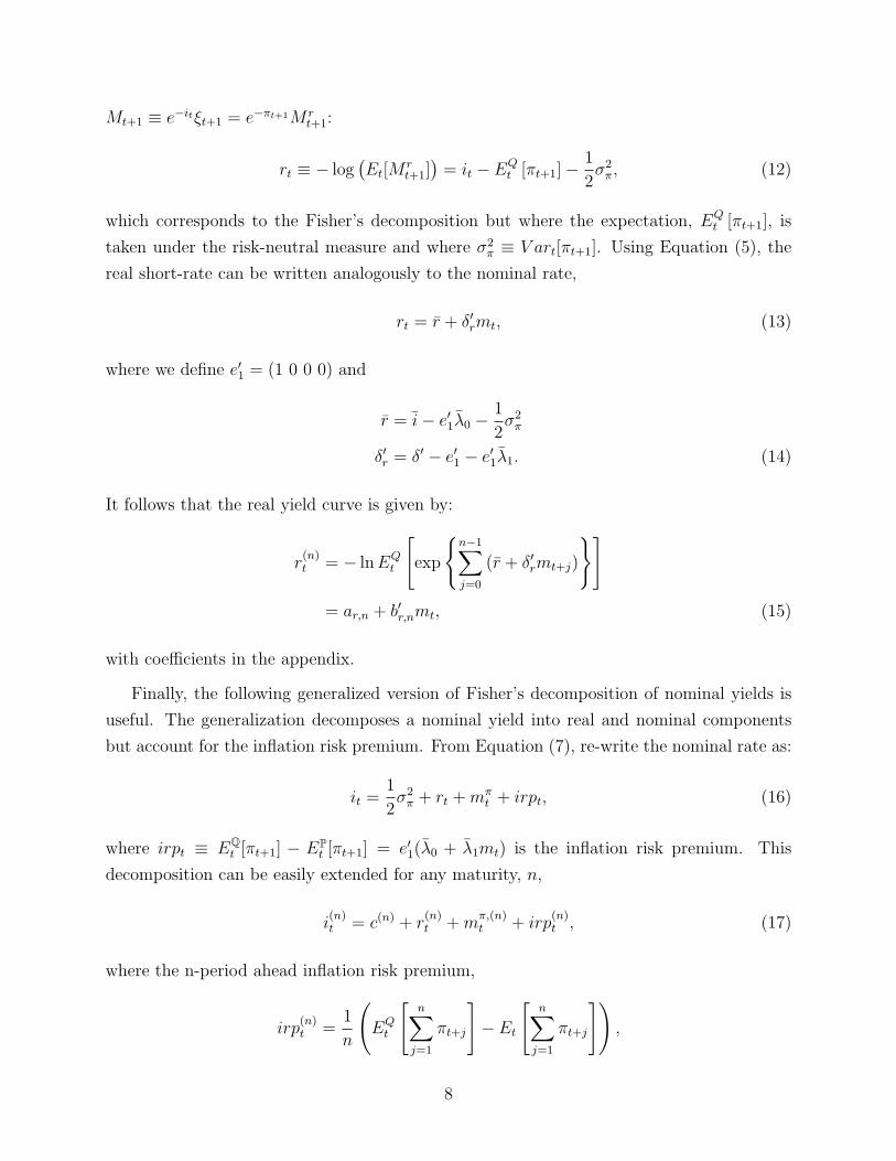
Mt+1 ≡ e−itξt+1 = e−πt+1M rt+1:

rt ≡ − log(Et[M

rt+1])= it − EQ

t [πt+1]−1

2σ2π, (12)

which corresponds to the Fisher’s decomposition but where the expectation, EQt [πt+1], is

taken under the risk-neutral measure and where σ2π ≡ V art[πt+1]. Using Equation (5), the

real short-rate can be written analogously to the nominal rate,

rt = r + δ′rmt, (13)

where we define e′1 = (1 0 0 0) and

r = i− e′1λ0 −1

2σ2π

δ′r = δ′ − e′1 − e′1λ1. (14)

It follows that the real yield curve is given by:

r(n)t = − lnEQ

t

[exp

{n−1∑j=0

(r + δ′rmt+j)

}]= ar,n + b′r,nmt, (15)

with coefficients in the appendix.

Finally, the following generalized version of Fisher’s decomposition of nominal yields is

useful. The generalization decomposes a nominal yield into real and nominal components

but account for the inflation risk premium. From Equation (7), re-write the nominal rate as:

it =1

2σ2π + rt +mπ

t + irpt, (16)

where irpt ≡ EQt [πt+1] − EP

t [πt+1] = e′1(λ0 + λ1mt) is the inflation risk premium. This

decomposition can be easily extended for any maturity, n,

i(n)t = c(n) + r

(n)t +m

π,(n)t + irp

(n)t , (17)

where the n-period ahead inflation risk premium,

irp(n)t =

1

n

(EQt

[n∑j=1

πt+j

]− Et

[n∑j=1

πt+j

]),

8

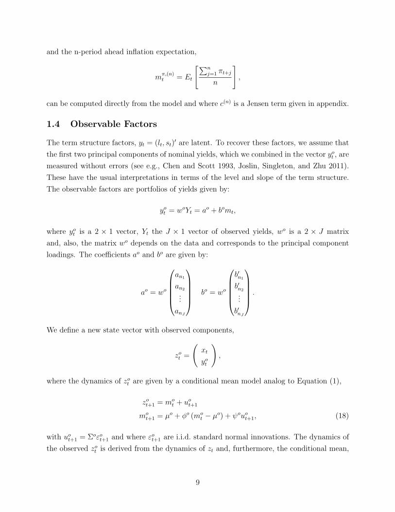
and the n-period ahead inflation expectation,

mπ,(n)t = Et

[∑nj=1 πt+j

n

],

can be computed directly from the model and where c(n) is a Jensen term given in appendix.

1.4 Observable Factors

The term structure factors, yt = (lt, st)′ are latent. To recover these factors, we assume that

the first two principal components of nominal yields, which we combined in the vector yot , are

measured without errors (see e.g., Chen and Scott 1993, Joslin, Singleton, and Zhu 2011).

These have the usual interpretations in terms of the level and slope of the term structure.

The observable factors are portfolios of yields given by:

yot = woYt = ao + bomt,

where yot is a 2 × 1 vector, Yt the J × 1 vector of observed yields, wo is a 2 × J matrix

and, also, the matrix wo depends on the data and corresponds to the principal component

loadings. The coefficients ao and bo are given by:

ao = wo

an1

an2

...

anJ

bo = wo

b′n1

b′n2

...

b′nJ

.

We define a new state vector with observed components,

zot =

(xt

yot

),

where the dynamics of zot are given by a conditional mean model analog to Equation (1),

zot+1 = mot + uot+1

mot+1 = µo + ϕo (mo

t − µo) + ψouot+1, (18)

with uot+1 = Σoεot+1 and where εot+1 are i.i.d. standard normal innovations. The dynamics of

the observed zot is derived from the dynamics of zt and, furthermore, the conditional mean,

9

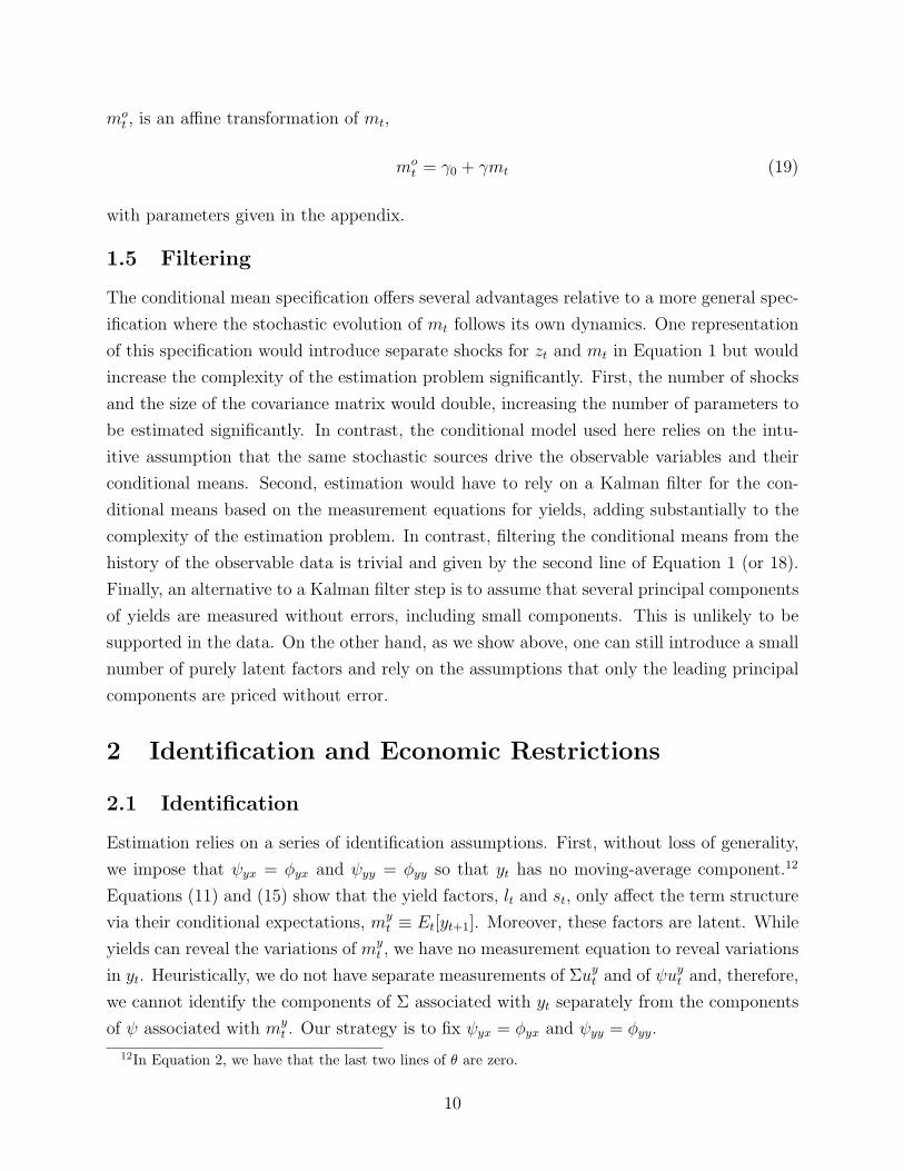
mot , is an affine transformation of mt,

mot = γ0 + γmt (19)

with parameters given in the appendix.

1.5 Filtering

The conditional mean specification offers several advantages relative to a more general spec-

ification where the stochastic evolution of mt follows its own dynamics. One representation

of this specification would introduce separate shocks for zt and mt in Equation 1 but would

increase the complexity of the estimation problem significantly. First, the number of shocks

and the size of the covariance matrix would double, increasing the number of parameters to

be estimated significantly. In contrast, the conditional model used here relies on the intu-

itive assumption that the same stochastic sources drive the observable variables and their

conditional means. Second, estimation would have to rely on a Kalman filter for the con-

ditional means based on the measurement equations for yields, adding substantially to the

complexity of the estimation problem. In contrast, filtering the conditional means from the

history of the observable data is trivial and given by the second line of Equation 1 (or 18).

Finally, an alternative to a Kalman filter step is to assume that several principal components

of yields are measured without errors, including small components. This is unlikely to be

supported in the data. On the other hand, as we show above, one can still introduce a small

number of purely latent factors and rely on the assumptions that only the leading principal

components are priced without error.

2 Identification and Economic Restrictions

2.1 Identification

Estimation relies on a series of identification assumptions. First, without loss of generality,

we impose that ψyx = ϕyx and ψyy = ϕyy so that yt has no moving-average component.12

Equations (11) and (15) show that the yield factors, lt and st, only affect the term structure

via their conditional expectations, myt ≡ Et[yt+1]. Moreover, these factors are latent. While

yields can reveal the variations of myt , we have no measurement equation to reveal variations

in yt. Heuristically, we do not have separate measurements of Σuyt and of ψuyt and, therefore,

we cannot identify the components of Σ associated with yt separately from the components

of ψ associated with myt . Our strategy is to fix ψyx = ϕyx and ψyy = ϕyy.

12In Equation 2, we have that the last two lines of θ are zero.

10

Second, we can rotate the latent state variables without changing the probability distribu-

tion of bond yields and, therefore, not all parameters can be identified separately. However,

results in Dai and Singleton (2000) imply that the identification of all the parameters can be

obtained using standard assumptions that we detail in Section 2.2.3. To see why standard

results apply, note that the dynamics of the factors entering the yield equation are standard

under the P and Q measures and given by:

mt+1 = µ+ ϕ (mt − µ) + ψut+1

mt+1 = µQ + ϕQ(mt − µQ

)+ ψQuQt+1,

respectively. Each corresponds to a VAR(1). The shifts between µ and µQ, between ϕ and

ϕQ, and between ψ and ψQ are standard and repeated here:

ωQ = ω + ψλ0

ϕQ = ϕ+ ψλ1

ψQ = ψ, (20)

where ωQ ≡(I4 − ϕQ

)µQ and ω ≡ (I4 − ϕ)µ. The parameter ψ determines the covariance

of mt shocks and remains the same under each measure as in standard gaussian models.

Third, the term structure of real yields is identified (in the econometric sense) from

nominal data. The only additional parameters arising from deriving the real curve are r

and δr, which determine the real short rate in terms of mt. But these parameters are given

from the connection between the nominal and real stochastic discount factors. Equation (14)

above, repeated here for convenience,

r = i− e′1λ0 −1

2σ2π

δ′r = δ′ − e′1 − e′1λ1.

shows that r is fixed given estimates of i, σ2π and λ0. Similarly, δr is determined by estimates

of δ and λ1. All these are identified from the nominal data using standard assumptions.

Clearly, the average short rate i, the volatility of inflation σ2π and the nominal short rate

coefficients δ can identified from the data. Equations (10) show that λ0 and λ1 are functions

of the parameters that determine the times-series and cross-section of yields.

11

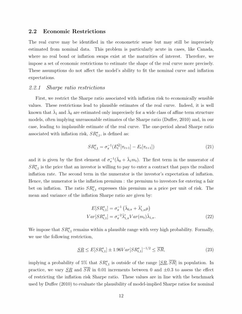
2.2 Economic Restrictions

The real curve may be identified in the econometric sense but may still be imprecisely

estimated from nominal data. This problem is particularly acute in cases, like Canada,

where no real bond or inflation swaps exist at the maturities of interest. Therefore, we

impose a set of economic restrictions to estimate the shape of the real curve more precisely.

These assumptions do not affect the model’s ability to fit the nominal curve and inflation

expectations.

2.2.1 Sharpe ratio restrictions

First, we restrict the Sharpe ratio associated with inflation risk to economically sensible

values. These restrictions lead to plausible estimates of the real curve. Indeed, it is well

known that λ1 and λ0 are estimated only imprecisely for a wide class of affine term structure

models, often implying unreasonable estimates of the Sharpe ratio (Duffee, 2010) and, in our

case, leading to implausible estimate of the real curve. The one-period ahead Sharpe ratio

associated with inflation risk, SRπt,1, is defined as:

SRπt,1 = σ−1

π (EQt [πt+1]− Et[πt+1]) (21)

and it is given by the first element of σ−1π (λ0 + λ1mt). The first term in the numerator of

SRπt,1 is the price that an investor is willing to pay to enter a contract that pays the realized

inflation rate. The second term in the numerator is the investor’s expectation of inflation.

Hence, the numerator is the inflation premium : the premium to investors for entering a fair

bet on inflation. The ratio SRπt,1 expresses this premium as a price per unit of risk. The

mean and variance of the inflation Sharpe ratio are given by:

E[SRπt,1] = σ−1

π

(λ0,π + λ′1,πµ

)V ar[SRπ

t,1] = σ−2π λ′1,πV ar(mt)λ1,π. (22)

We impose that SRπt,1 remains within a plausible range with very high probability. Formally,

we use the following restriction,

SR ≤ E[SRπt,1]± 1.96V ar[SRπ

t,1]−1/2 ≤ SR, (23)

implying a probability of 5% that SRπt,1 is outside of the range [SR, SR] in population. In

practice, we vary SR and SR in 0.01 increments between 0 and ±0.3 to assess the effect

of restricting the inflation risk Sharpe ratio. These values are in line with the benchmark

used by Duffee (2010) to evaluate the plausibility of model-implied Sharpe ratios for nominal

12

bond returns in the US.13

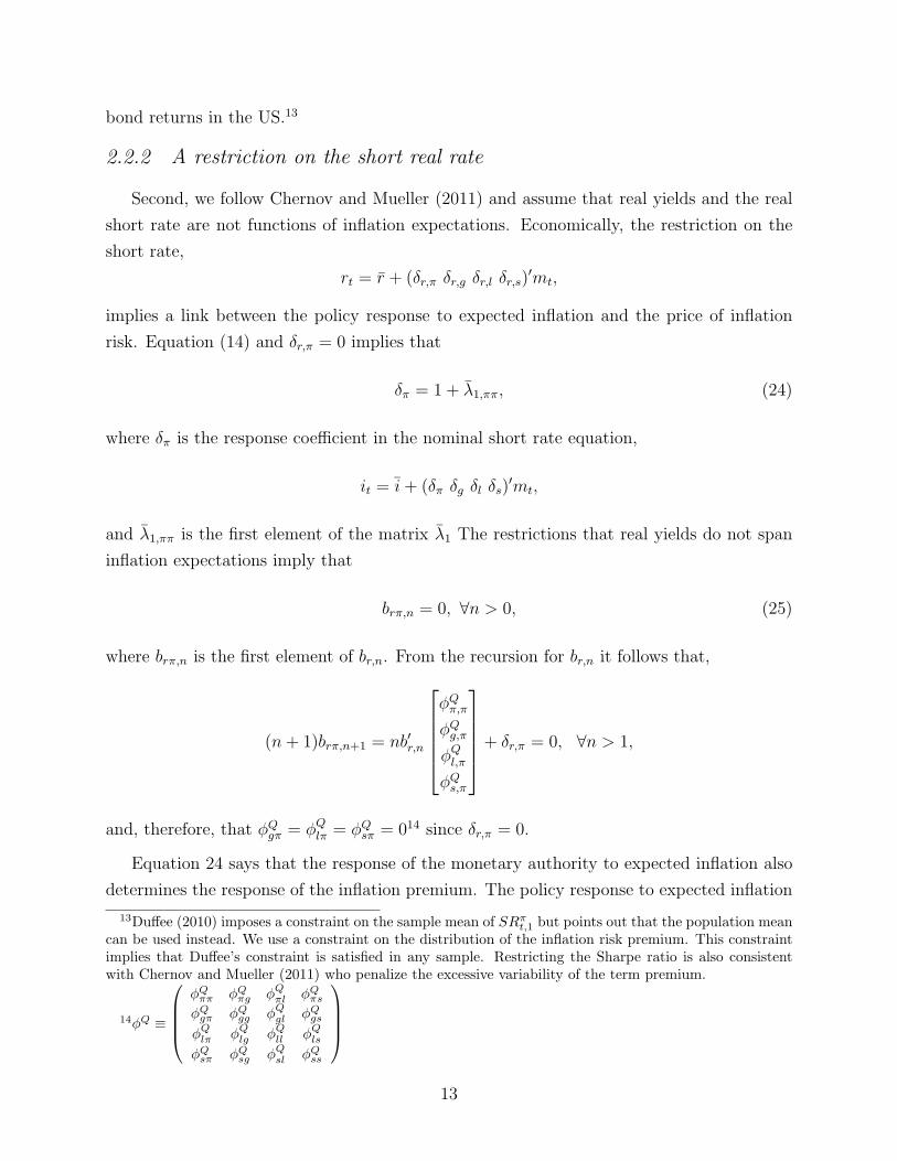
2.2.2 A restriction on the short real rate

Second, we follow Chernov and Mueller (2011) and assume that real yields and the real

short rate are not functions of inflation expectations. Economically, the restriction on the

short rate,

rt = r + (δr,π δr,g δr,l δr,s)′mt,

implies a link between the policy response to expected inflation and the price of inflation

risk. Equation (14) and δr,π = 0 implies that

δπ = 1 + λ1,ππ, (24)

where δπ is the response coefficient in the nominal short rate equation,

it = i+ (δπ δg δl δs)′mt,

and λ1,ππ is the first element of the matrix λ1 The restrictions that real yields do not span

inflation expectations imply that

brπ,n = 0, ∀n > 0, (25)

where brπ,n is the first element of br,n. From the recursion for br,n it follows that,

(n+ 1)brπ,n+1 = nb′r,n

ϕQπ,π

ϕQg,π

ϕQl,πϕQs,π

+ δr,π = 0, ∀n > 1,

and, therefore, that ϕQgπ = ϕQlπ = ϕQsπ = 014 since δr,π = 0.

Equation 24 says that the response of the monetary authority to expected inflation also

determines the response of the inflation premium. The policy response to expected inflation

13Duffee (2010) imposes a constraint on the sample mean of SRπt,1 but points out that the population mean

can be used instead. We use a constraint on the distribution of the inflation risk premium. This constraintimplies that Duffee’s constraint is satisfied in any sample. Restricting the Sharpe ratio is also consistentwith Chernov and Mueller (2011) who penalize the excessive variability of the term premium.

14ϕQ ≡

ϕQππ ϕQπg ϕQπl ϕQπsϕQgπ ϕQgg ϕQgl ϕQgsϕQlπ ϕQlg ϕQll ϕQlsϕQsπ ϕQsg ϕQsl ϕQss

13

affects the contemporaneous short rate via the compensation for inflation risk. For instance,

if the policy response is more than one-for-one, and monetary policy is stabilizing with

respect to inflation, then the inflation premium declines when the policy rate is lowered in

response to lower inflation expectations. Therefore, the bounds on the inflation Sharpe ratio

may limit the role of expected inflation in the evolution, which affects the estimate of the

expected inflation response coefficient. We explore this important question in the empirical

section.

2.2.3 Nelson-Siegel representation of real yields

Third, we impose that the loadings of the yield factors, yt, correspond to the level and

slope loadings in the Nelson-Siegel representation (Nelson and Siegel 1987, Christensen,

Diebold, and Rudebusch 2007). Specifically, we find conditions such that real yields are

given by,

brl,n = 1; brs,n = 1−e−nλ

nλmst ; λ > 0. (26)

This representation is parsimonious and widely used to model interest rates. It also directly

justifies that we label lt and st the level and slope factor, respectively. Following Christensen,

Lopez, and Rudebusch (2010), we do not include a curvature factor to model the real curve.15

The parameter λ controls the steepness of the slope and is estimated jointly with other

parameters.

Equation 26 implies that ϕQxy = 0, and

δy =

[1

1−e−λ

λ

]; ϕQyy =

[1 0

0 e−λ

]; ϕQxy ≡

(ϕQπl ϕQπs

ϕQgl ϕQgg;

)=

[0 0

0 0

]. (27)

Note that the Nelson-Siegel representation identifies the scale, the sign and the ordering of

the latent factors via its implications for δy. We fix λl0 = λs0 = 0 to identify the level of the

latent term structure factors.16

2.2.4 Summary of the restrictions

For convenience, we summarize here the restrictions discussed in this section. Parameters

of the short real and nominal rates are given by:

δ′r =[0 δr,g 1 1−e−λ

λ

], (28)

15This is a simplification of the original NS representation. Christensen, Lopez, and Rudebusch (2010)find that a level and slope factors are sufficient to model the term structure of TIPS yields in the US.

16See Christensen et al. (2007) for a discussion of identification assumptions in the context of affine modelswith a Nelson-Siegel representation. We define λ′0 ≡ (λ0,π λ0,g λ0,l λ0,s).

14

parameters of the the P-dynamics are given by:

µ =

[µx

µy

]ϕ =

[ϕxx ϕxy

ϕyx ϕyy

]ψ =

[ψxx ψxy

ϕyx ϕyy

], (29)

and parameters of the the Q-dynamics are given by:

µQ =

[µQx

µQy

]ϕQ =

[ϕQxx 0

ϕQyx ϕQyy

]ψQ =

[ψxx ψxy

ϕQyx ϕQyy

], (30)

with ϕQyy given in Equation 27 and ϕQgπ = ϕQlπ = ϕQsπ = 0. The parameters under each measure

are also linked via Equation 10 with the additional restrictions that λl0 = λs0 = 0.

3 Data and Estimation

3.1 Data

The sample is monthly and includes the unemployment rate, gt, and the (total) inflation

rate, π = ln pt+1

pt, from January 1986 until December 2011. We use yields on zero-coupon

bonds with maturities of 3, 6, 9, 12 and 18 months as well as 2, 3, 4, 7, 8, 9, 10 years over

the same sample. We also use data from surveys of professional forecasters by Consensus

Economics (CE). On the last month of every quarter, the survey asks for a forecast of the

average of year-over-year inflation rates across all months in a given quarter. The survey

covers the remaining quarters of the current calendar year, and every quarter of the following

calendar year. We use the first five quarters to obtain a balanced panel since longer horizon

forecasts are available only irregularly.17

3.2 Likelihood

3.2.1 State dynamics

First, we estimate parameters of the state dynamics based on the likelihood of zot , ex-

cluding the survey data and without imposing the no-arbitrage restrictions. The conditional

17The inflation rate is computed from the Canadian seasonally adjusted all items consumer price index(StatCan Table 326-0020) and the unemployment is also seasonally adjusted (StatCan 282-0089). Zero-coupon yields are available from the Bank of Canada’s web site. The survey is taken on the second weekof each month but the inflation forecasts are only updated quarterly. StatCan releases inflation data at theend of each month and with a one-month lag. Hence, survey participants on the second week of March knowthe inflation rate up to the month of January.

15

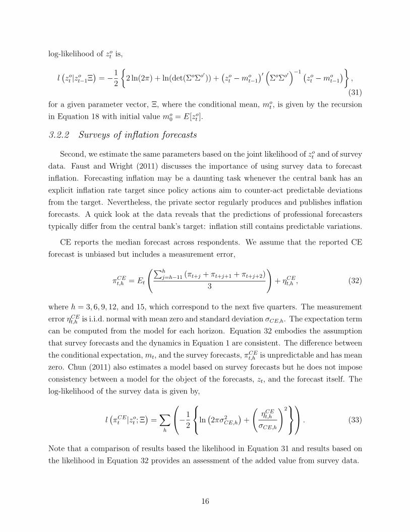
log-likelihood of zot is,

l(zot |zot−1Ξ

)= −1

2

{2 ln(2π) + ln(det(ΣoΣo′)) +

(zot −mo

t−1

)′ (ΣoΣo′

)−1 (zot −mo

t−1

)},

(31)

for a given parameter vector, Ξ, where the conditional mean, mot , is given by the recursion

in Equation 18 with initial value mo0 = E[zot ].

3.2.2 Surveys of inflation forecasts

Second, we estimate the same parameters based on the joint likelihood of zot and of survey

data. Faust and Wright (2011) discusses the importance of using survey data to forecast

inflation. Forecasting inflation may be a daunting task whenever the central bank has an

explicit inflation rate target since policy actions aim to counter-act predictable deviations

from the target. Nevertheless, the private sector regularly produces and publishes inflation

forecasts. A quick look at the data reveals that the predictions of professional forecasters

typically differ from the central bank’s target: inflation still contains predictable variations.

CE reports the median forecast across respondents. We assume that the reported CE

forecast is unbiased but includes a measurement error,

πCEt,h = Et

(∑hj=h−11 (πt+j + πt+j+1 + πt+j+2)

3

)+ ηCEt,h , (32)

where h = 3, 6, 9, 12, and 15, which correspond to the next five quarters. The measurement

error ηCEt,h is i.i.d. normal with mean zero and standard deviation σCE,h. The expectation term

can be computed from the model for each horizon. Equation 32 embodies the assumption

that survey forecasts and the dynamics in Equation 1 are consistent. The difference between

the conditional expectation, mt, and the survey forecasts, πCEt,h is unpredictable and has mean

zero. Chun (2011) also estimates a model based on survey forecasts but he does not impose

consistency between a model for the object of the forecasts, zt, and the forecast itself. The

log-likelihood of the survey data is given by,

l(πCEt |zot ; Ξ

)=∑h

−1

2

ln(2πσ2

CE,h

)+

(ηCEt,hσCE,h

)2 . (33)

Note that a comparison of results based the likelihood in Equation 31 and results based on

the likelihood in Equation 32 provides an assessment of the added value from survey data.

16

3.2.3 Yields cross-section

Third, we impose the no-arbitrage restrictions and estimate parameters of the historical

and of the risk-neutral dynamics jointly using all yields and survey data. The yield data

include N ≤ J − 2 combinations of yields, Y et , that are measured with errors. The n-th

combination of yields is given by:

Y en,t = wenYt = aen + benm

ot + ηen,t,

where ηen,t is i.i.d. normal with mean zero and standard deviation σe,n.18. The coefficients

are given by:

ae = we(a+ bγ0)

be = webγ,

and we is an N × J matrix and the conditional log-likelihood of Y et,n is given by

l(Y et,n|zot ; Ξ

)=∑n

(−1

2

{ln(2πσ2

e,n

)+

(ηet,nσe,n

)2})

. (34)

Adding the likelihood of yields allows for the estimation of the risk-neutral parameters and

delivers estimates of the inflation risk premium and real yields. We rely on the assumption

that inflation expectations embodied in yields corresponds with model expectations.

3.2.4 Combining Likelihood

We nest the likelihoods of the data together and write:

L(Ξ) =T∑t=1

(1i(z

ot )l(zot |zot−1; Ξ

)+ 1i(π

CEt )l

(πCEt |zot ; Ξ

)+ 1i(Y

et )l (Y

et |zot ; Ξ)

)(35)

where zo0 = µo. The indicator function 1i(zot ) is equal to one if model i is estimated using

the likelihood of zot . We estimate various models using zot data (i.e., 1i(zot ) = 1), some

models also use survey data (i.e., 1i(πCEt ) = 1)and, in addition, models that impose the

absence of arbitrage opportunity also use all the yield data (i.e., 1i(Yet ) = 1). We have that

the indicator 1i(πCEt ) is equal to 1 every three months since survey data is only available

quarterly. In all cases, we fix parameters controlling the unconditional means of the state

variables to their respective sample averages and impose the usual stationarity conditions on

18We set N=5, and we assume that Y et is constituted of principal components 3 to 7.

17

the eigenvalues of ϕ. We also impose the stationarity of the macro variables under Q. Errors

in fitting zot may receive a greater weight in the maximization of the likelihood. But this

also depends on the relative magnitude of the variance of state innovations and the variance

of survey measurement errors.

4 Decomposing Nominal Yields

We estimate the historical and risk-neutral dynamics of zt based on the joint likelihood, L(Ξ)

where −SR = SR = 0.20. This is a reasonable value given existing estimates. For instance,

Duffee (2011) finds that the maximum Sharpe ratio from a porfolio of US Treasury bonds

and bills is 0.23 on average. Moreover, varying this parameter does not affect inflation

expectations measured from the model. Figure 5 compares forecast error RMSEs at two

horizons: one month and one year, across a range of values for the Sharpe ratio bounds from

0 to 0.30. We report the ratio of the forecast RMSE relative to the case where the bound

is zero and the 1-month inflation risk premium is constant at zero. The 1-month RMSE

decreases as we move away from a zero inflation risk premium. The maximum likelihood

estimator explicitly minimizes the one-month forecast variance. In contrast, the one-year

forecast RMSE remains essentially constant as we increase the bound. Overall, Figure 5

suggests that freeing the Sharpe ratio constraint leads to an over-fitting of the 1-month

inflation forecast at no benefit for other horizons. Hence, we focus the analysis for the case

where SR = SR = 0.20. Table 1 displays the standard deviations of survey measurement

errors and of yield pricing errors for this case. The model fits the survey forecasts closely.

The standard deviations range between 1.1 and 1.8 basis point annually. Similarly, the

model fits the yields closely. The first two principal components of yields are priced exactly

by construction and the standard deviations for the remaining five components range from

0.1 to 1.1 basis point annually.

4.1 Measuring Inflation Expectations

Figure 7 displays the time series of expected inflation at horizons of 3 months, 1 year, 2

years and 5 years. It shows the decline in inflation expectations from a level of between

3% and 4% in the late 1980s to a level around 2% in the more recent period. This is

consistent with the new inflation targeting regime initiated in the 1990s. Figure 7 also shows

the strong pro-cyclical behavior of expected inflation: expectations decrease markedly when

the unemployment rate rises. Finally, the slope of inflation expectations across different

horizons changes sign through the cycle. Short-run inflation expectations stand below long-

run inflation expectations when unemployment is high, and vice-versa when unemployment

18

is low.

A natural criteria to assess whether we obtain good measurements of expected inflation is

their accuracy as inflation forecasts. Hence, we compare the out-of-sample forecast RMSEs

from our preferred model with results from a battery of alternatives. We estimate each

model with data until December 1991, compute inflation forecasts for horizons up to two

years ahead and compute forecast errors against the realized values of inflation. Then,

the estimation window is lengthened by one month, new forecasts and forecast errors are

produced, and the exercise is repeated until we reach the end of the sample.

With the exception of three simple univariate alternatives, we consider a variety of mod-

els that are nested in the framework of Equation 1 and which can be estimated from the

likelihood given by Equation 35. First, we estimate the following univariate models:

(i) Random walk models

· RW1 : Et

(∑hj=1 πt+j

h

)= πt

· RW2 : Et

(∑hj=1 πt+j

h

)= 1

12

∑11j=0 πt−j

(ii) Stationary models

· AR : mπt+1 = µπ + ϕπ(πt+1 − µπ)

· ARMA : mπt+1 = µπ + ϕπ(m

πt − µπ) + ψπu

πt+1

· S-ARMA : mπt+1 = µπ + ϕπ(m

πt − µπ) + umt+1.

RW1 and RW2 are simple random walk models. The AR(1) and ARMA(1,1) models are

nested in the framework of this paper, and the stochastic mean model, S-ARMA(1,1) allows

for an additional shock umt+1 to the conditional mean mπt+1. We also estimate the following

multivariate models combining the inflation rate and the unemployment rate, x′t = (πt, gt),

but excluding the yield factors, yt.

(iii) Inflation and Unemployment

· VAR-U: mxt+1 = µx + ϕx(xt+1 − µπ)

· VARMA-U: mxt+1 = µx + ϕx(m

xt − µπ) + ψxu

πt+1,

then we expand the system to include the yield factors,

(iv) Inflation, Unemployment, Level and Slope

19

· VAR-UL and VAR-ULS : mt+1 = µ+ ϕ(zt+1 − µ)

· VARMA-UL and VARMA-ULS : mt+1 = µ+ ϕ(mt − µ) + ψut.

Table 2 displays the relative RMSEs compared to results from the AR(1) across all

models. Panel A presents results from forecasts at the quarterly frequency to compare

with survey forecasts. Panel B presents monthly forecast RMSEs. The results yield several

messages. First, different types of model can match the accuracy of out-of-sample quarterly

survey forecasts. This result is consistent with the results in Faust and Wright (2011) for the

US but contrasts with those of Ang, Bekaert, and Wei (2008). Second, the conditional mean

model combining the macro variables and two yield factors, level and slope, delivers by far

the best performance at the monthly frequency. This is especially true at longer horizons

(see last column in Panel B).

4.1.1 The added-value of survey’s information

Using survey data is essential, and this is especially true for more sophisticated models.

Table 3 displays the ratio of the forecast RMSEs obtained when using survey data to the

RMSEs obtained without surveys. For instance, including surveys improves forecast RMSEs

of the VAR-ULS model by 22% and that of the VARMA-ULS model by 33%. Using survey

data is particularly useful for when we move from multivariate VAR to VARMA models

where the increase in the number of parameters is more important.

Unsurprisingly, the information from quarterly surveys improves quarterly inflation fore-

casts. For instance, RMSEs typically decrease by 5-10% at the 1-quarter horizon and by

15-30% at longer horizons. More importantly, using quarterly surveys also delivers sub-

stantial RMSE improvements for monthly forecasts. The evidence is particularly stark for

conditional mean models and at long horizons. For instance, including surveys improves the

3-month forecast RMSE from the VARMA-ULS model by 5% but improves the 2-year ahead

RMSE by 24%. This arises even if the accuracy of survey forecasts deteriorates with the

horizon.

Surveys provide an effective counter-weight to the loss of parsimony associated with

conditional mean models (i.e., moving from a VAR(1) to a VARMA(1,1) model). Estimates

that neglect survey data suffer from substantial bias and small-sample sampling errors due

to its persistence and to the presence of a volatile transitory component (Kim 2007, Kim and

Orphanides 2012). Adding surveys to the measurement equations effectively lengthens the

sample. The improvements can only arise from better estimates of the underlying dynamics

and not from some over-fitting of the survey forecasts. There are no surveys at the 2-year

horizon.

20

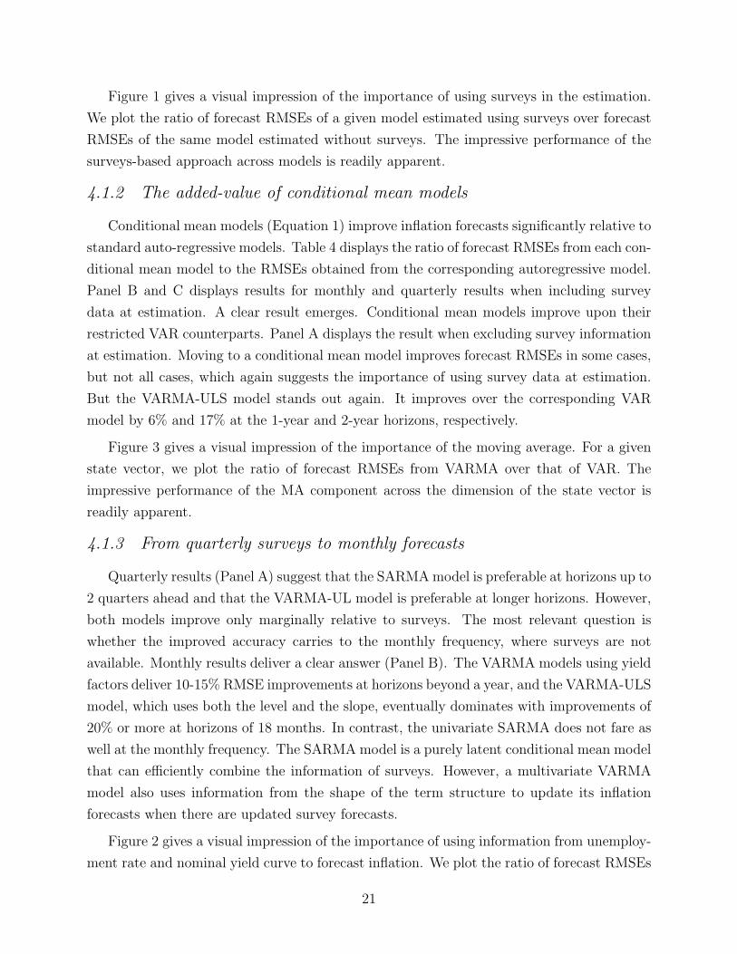
Figure 1 gives a visual impression of the importance of using surveys in the estimation.

We plot the ratio of forecast RMSEs of a given model estimated using surveys over forecast

RMSEs of the same model estimated without surveys. The impressive performance of the

surveys-based approach across models is readily apparent.

4.1.2 The added-value of conditional mean models

Conditional mean models (Equation 1) improve inflation forecasts significantly relative to

standard auto-regressive models. Table 4 displays the ratio of forecast RMSEs from each con-

ditional mean model to the RMSEs obtained from the corresponding autoregressive model.

Panel B and C displays results for monthly and quarterly results when including survey

data at estimation. A clear result emerges. Conditional mean models improve upon their

restricted VAR counterparts. Panel A displays the result when excluding survey information

at estimation. Moving to a conditional mean model improves forecast RMSEs in some cases,

but not all cases, which again suggests the importance of using survey data at estimation.

But the VARMA-ULS model stands out again. It improves over the corresponding VAR

model by 6% and 17% at the 1-year and 2-year horizons, respectively.

Figure 3 gives a visual impression of the importance of the moving average. For a given

state vector, we plot the ratio of forecast RMSEs from VARMA over that of VAR. The

impressive performance of the MA component across the dimension of the state vector is

readily apparent.

4.1.3 From quarterly surveys to monthly forecasts

Quarterly results (Panel A) suggest that the SARMAmodel is preferable at horizons up to

2 quarters ahead and that the VARMA-UL model is preferable at longer horizons. However,

both models improve only marginally relative to surveys. The most relevant question is

whether the improved accuracy carries to the monthly frequency, where surveys are not

available. Monthly results deliver a clear answer (Panel B). The VARMA models using yield

factors deliver 10-15% RMSE improvements at horizons beyond a year, and the VARMA-ULS

model, which uses both the level and the slope, eventually dominates with improvements of

20% or more at horizons of 18 months. In contrast, the univariate SARMA does not fare as

well at the monthly frequency. The SARMA model is a purely latent conditional mean model

that can efficiently combine the information of surveys. However, a multivariate VARMA

model also uses information from the shape of the term structure to update its inflation

forecasts when there are updated survey forecasts.

Figure 2 gives a visual impression of the importance of using information from unemploy-

ment rate and nominal yield curve to forecast inflation. We plot the ratio of forecast RMSEs

21

of a given model over that of an AR(1). The impressive performance of adding information

from macroeconomic and nominal yield data is readily apparent. The univariate ARMA

model on inflation is dominated by a bivariate VARMA model on inflation and unemploy-

ment rate, which in turn is dominated by a VARMA model on inflation, unemployment rate

and the level of the nominal yield curve. Finally the most flexible model, VARMA model on

inflation, unemployment rate, level and slope of the nominal yield curve, is superior to all

the other models. This, again, highlight the importance of using information from nominal

yield to update our anticipation of inflation.

4.1.4 Can survey forecasts be improved?

No model systematically improves upon the accuracy of survey forecasts. Table 5 displays

the ratio of each model’s forecast RMSEs relative to the surveys’ RMSEs. Most models

perform reasonably well though. The worst performers are the AR and VAR-U model, with,

at best, a 1-2% improvement as some horizons and, at worse, a 8-9% deterioration. On the

other hand, a VARMAmodel using yield factors and estimated based on survey data matches

or improves survey RMSEs. Figure 6 compares the model forecasts with the CE forecasts

and with the realized values of inflation at horizons of 1, 2, 3 and 4 quarters. One-quarter

ahead model-forecasts are very close to CE forecasts. Both predict realized inflation very

well. The same is true for 2-quarter ahead forecasts but with a small deterioration. Model-

implied and CE forecasts are still close to each others at longer horizons. This provides

further confirmation that the dynamic term structure model captures inflation expectations

accurately. In contrast, Ang, Bekaert, and Wei (2007) and Faust and Wright (2011) conclude

that no model can match the accuracy of survey forecasts in US data.19

Figure 4 gives a visual impression of the CE forecasts accuracy. We plot the ratio of

the forecast RMSEs of a given model over that of CE forecast RMSEs. All the models do

as well as CE forecasts at the quarterly frequency but, conversely, CE forecasts are hard to

outperform when available.

4.2 The Effect of Yields on Inflation and Unemployment

This Section explores the mechanism which allows our preferred specification to out-perform

more parsimonious models out-of-sample. The answer lies in the information content of

the yield curve. Consider the implications for the dynamics of inflation and unemployment

19Survey forecasts exhibit systematic errors ex-post. Ang, Bekaert, and Wei (2007) show that linear ornon-linear adjustment do not improve unadjusted out-of-sample inflation forecasts.

22

expectations,

mx,t = ϕxx(mx,t−1 − µx) + ϕxy(my,t−1 − µy) + ψxxux,t + ψxyuy,t. (36)

Last period’s expectations for today’s values of the macro variables, mx,t−1, and last period’s

expectations of today’s shape of the yield curve, my,t−1, respectively, affect the update of

inflation expectation differently than the corresponding surprise components, ux,t and uy,t,

respectively. This is a distinctive feature of a conditional mean model. Contrast Equation 36

with the corresponding equation in a VAR model,

mx,t ≡ Et[xt+1]

= ϕxx(xt − µx) + ϕxy(yt − µy)

= ϕxx(mx,t−1 − µx) + ϕxy(my,t−1 − µy) + ϕxxux,t + ϕxyuy,t,

where ϕ = ψ and last period’s expectations for today’s state variables, mt−1, have the same

effect on the updated expectation as the innovations ut.

But the estimates imply a remarkable difference between ψ and ϕ. Table 6 displays

parameter estimates. The matrices ϕ and ψ are given in Panel (A) with standard errors in

parenthesis. First, the estimate of ϕ implies that inflation expectations and unemployment

expectations are persistent (ϕπ = 0.84 and ϕg = 0.96). Second, the first column of ψ

is insignificant and very close to zero in magnitude. In other words, the innovation in

current inflation has almost no effect on the conditional expectations of inflation and of

unemployment. Hence, the intuition from Kim (2007) that inflation combines a persistent

conditional mean component with transitory noise carries over in our multivariate context.

Third, since inflation innovations have little effect, inflation expectation updates are driven

by innovations in the other variables. Their effect is given on the first line of ψ. Innovations

in the unemployment rate, the level of yields and the slope of yields each have large and

significant effects on inflation expectation updates. For instance, a one-standard deviation

surprise increase in the level or a similar surprise decrease in the slope of the yield curve

lowers inflation expectations by 0.35% and by 0.13%, respectively (all else constant). Fourth,

in contrast with the effect of innovations, expected increases in the level of the curve are

associated with expected increases in inflation. The initial effects of expectation changes are

smaller but cumulate over time via the persistence of the level and slope factors. The effect

of expected changes in the slope is insignificant.

The effects are consistent with intuition. Monetary policy shocks affect the inflation

expectation downward. Yet, predictable increases in expected inflation are positively cor-

23

related with the level and slope of the yield curve. The conditional mean model separates

these two effects parsimoniously. Similarly, the expected and surprise components of today’s

yield curve do not have the same effect on the expected unemployment rate. In particular,

a surprise decrease in the slope of the yield curve is associated with a significant increase of

the expected unemployment rate. On the other hand, an expected change in the slope bears

almost no effect on the expected unemployment rate. This is consistent with results from

Ang et al. (2006) showing that the level of interest rate is the best predictors of future real

activity in the context of a terms structure model.

Finally, the standard deviations and correlations implied from the estimate of the covari-

ance matrix ΣΣ′ and ψΣΣ′ψ′ are given in Panel (B) (standard deviations are given on the

diagonal). Again, while the correlations between inflation innovations and other innovations

are low, the correlations between updates to inflations expectations and updates to expec-

tations of other variables are high. This highlights the role of the matrix ψ in the update of

expected inflation.

4.3 Real Yields and the Inflation Risk Premium

Figure 8 displays the loadings on nominal yields. By construction, the level factor has a

constant unit loading and the loadings of the slope factor decreases smoothly with matu-

rity. The effect of macro variables on yields is most important at shorter maturities. The

generalized Fisher equation,

i(n)t = c(n) +m

π,(n)t + r

(n)t + irp

(n)t , (37)

derived in Section 1 (see Equation 17), shows that a successful decomposition of yields

involves three components: a real yield, expected inflation and the inflation risk premium.

The previous Section established that the model delivers an accurate measure of mπ,(n)t ,

which in turns implies that the model delivers an accurate measure of the sum of the real

yield and the inflation risk premium, r(n)t + irp

(n)t . Heuristically, we can then subtract the

Jensen term and our measure of mπ,(n)t from both sides of the decomposition,

i(n)t − c(n) −m

π,(n)t = r

(n)t + irp

(n)t . (38)

and focus on estimates of the remaining components from the model, relying on the restric-

tions imposed on the prices of risk to obtain an accurate decomposition of the sum on the

right hand side.

Table 7 displays summary statistics of nominal yields, real yields, inflation expectations

24

and the inflation risk premiums computed from the model across a range of maturities

between three months and five years. The average nominal yield curve is upward sloping –

with an average slope close to 0.85%. But the relatively low average slope hides substantial

variation over the business cycle. The average volatility is downward sloping, ranging from

3.27% to 2.56%. The average slope and volatility of the nominal curve is attributable to the

level and volatility of the real curve. Moreover, their persistence is similar. Average expected

inflation is mostly flat across maturities, slightly above 2% across the sample, adding little

to the average slope. The inflation risk premium averages between 0.44% and 0.57% with an

upward slope, adding 13 bps to the difference between the slopes of real and nominal yields.

Figure 9 displays the time-series of each component of yields – the real yield, expected

inflation and inflation risk premium – for maturities of three month, one year, two years

and five years. By and large, the large business cycle variations in the nominal yield curve

are attributed to variations in the underlying real curve. The inflation risk premium is the

least volatile component of nominal yields at short maturities and where it follows closely

variations of expected inflation. The contribution of the inflation risk premium increases

with the maturity and the sources of its variations also change. Figure 10 displays the

contribution of each component of mt to the variations of the 2-year inflation risk premium.

At this horizon, the expected inflation and the slope factor have little effect on the inflation

risk premium. Instead, the premium is high when unemployment is high or when the level

of the yield curve is low– in relatively poor states of the economy.20

What is the source of risk behind the importance of the unemployment rate and the

level factor for the variation of the longer-horizon inflation risk premium? The loadings on

1-month the inflation risk premium in Figure 10 combine the price of risk with the covariance

matrix,

mQt −mt = (ΣΣ′)(λ0 + λ1mt)

since the effect of each component on the inflation risk premium is determined by the product

(ΣΣ′)λ1. A similar decomposition obtains at longer horizons but where the covariance matrix

and the price of risk coefficients depend on the horizon.

Panel (A) and Panel (B) of Figure 12 decomposes the effect of unemployment and of

20Interestingly, the inflation risk premium has been persistently negative in the short period from thebeginning of the sample until the Bank of Canada announced a new inflation targeting regime. This isconsistent with an interpretation where an increase in expected inflation does not announce a tighteningphase by the central bank due to an insufficient response to inflation. Exposures to inflation risk becomehedges.This may also arise, for instance, if the representative agent has Epstein-Zin preferences. Inflation isalways risky for a CRRA agent - inflation enters negatively in the SDF. However, higher inflation may leadto revisions of the continuation value in the Epstein-Zin SDF. In this context, changes in the sign of theinflation risk premium require changes in the covariance between current inflation and future consumptiongrowth.

25

the level factor, respectively, on the 2-year inflation risk premium. Each line of Panel (A)

draws the products of the effect of unemployment rate on the price of risk of a given variable

with the covariance of this variable with inflation innovations across different horizons. The

results show that inflation risk is the main channel behind the role of unemployment in the

inflation risk premium. Across different horizons, the effects of the level factor and of the

unemployment rate on the inflation risk premium work primarily through their effects on the

price of inflation risk. The pricing kernel gives lower value to payoffs in states with inflation

shocks, and the value decreases when expected unemployment is higher or the level of the

curve is lower.

Conclusion

Our results show that the main conclusion in Faust and Wright (2011) carries over to the case

of Canada : using information from CE allows even simple models to capture the predictive

content from survey. We also show how to combine the conditional mean representation in

Fiorentini and Sentana (1998) with survey and yield data to produce superior out-of-sample

forecasts even when no updated survey is available. Finally, we develop a dynamic term

structure model to decompose the yield curve into real yields, inflation expectations, and

the inflation risk premium at different maturities.

We leave for future research several important extensions. First, we focus on short hori-

zons - typically less than two years. Longer horizon forecasts must handle shifting endpoints

(Kozicki and Tinsley, 2001) since the long-horizon inflation forecasts have declined in the

first half of the sample. But we must also accommodate long episodes where the median

long-horizon CE forecast remains constant. Second, our analysis relies on models with con-

stant variance. Still, a large literature studies the relationship between uncertainty about

inflation and future inflation. Moreover, a recent literature sees the dispersion of inflation

forecasts among survey respondents as an important signal of inflation risk. Extending the

model to account for time-varying uncertainty may help us identify a more fundamental role

of inflation risk using yield data. Finally, we focused on inflation forecasts. But conditional

forecasts of future inflation rates are not independent of forecasts of future unemployment

rates (or other macro variables). Extending our approach to include CE forecasts of unem-

ployment could help identify the dynamic relationships between economic activity, inflation

and risk as perceived by bond investors.

26

References

Ajello, A., L. Benzoni, and O. Chyruk (2012). Core and ’crust’: Consumer prices and theterm structure of interest rates. Federal Reserve Bank of Chicago.

Amano, R. and S. Murchison (2006). Factor-market structure, shifting inflation targets, andthe new keynesian phillips curve. In Issues in Inflation Targeting, pp. 89–109. Bank ofCanada.

Ang, A., G. Bekaert, and M. Wei (2007). Do macro variables, asset markets, or surveysforecast inflation better? Journal of Monetary Economics 54 (4), 1163 – 1212.

Ang, A., G. Bekaert, and M. Wei (2008). The term structure of real rates and expectedinflation. The Journal of Finance 63 (2), 797–849.

Ang, A., S. Dong, and M. Piazzesi (2007). No-arbitrage taylor rules. Working Paper 13448,National Bureau of Economic Research.

Ang, A. and M. Piazzesi (2003). A no-arbitrage vector autoregression of term structure dy-namics with macroeconomic and latent variables. Journal of Monetary Economics 50 (4),745 – 787.

Ang, A., M. Piazzesi, and M. Wei (2006). What does the yield curve tell us about gdpgrowth? Journal of Econometrics 131 (12), 359–403.

Bansal, R. and I. Shaliastovich (2010). A long-run risks explanation of predictability puzzlesin bond and currency markets. The Wharton School of Business, University of Pennsyl-vania.

Bansal, R. and A. Yaron (2004). Risks for the long run: A potential resolution of assetpricing puzzles. The Journal of Finance 59, 1481–1509.

Buraschi, A. and A. Jiltsov (2005). Inflation risk premia and the expectations hypothesis.Journal of Financial Economics 75 (2), 429–490.

Campbell, J., R. Shiller, and L. Viceira (2009). Understanding inflation-indexed bond mar-kets. Working Paper 15014.

Chen, R.-R. and L. Scott (1993). Maximum likelihood estimation for a multifactor equi-librium model of the term structure of interest rates. The Journal of Fixed Income 3,14–31.

Chernov, M. and P. Mueller (2011). The term structure of inflation expectations. Journalof Financial Economics . forthcoming.

Christensen, J., F. Diebold, and G. Rudebusch (2007). The affine arbitrage-free class ofNelson-Siegel term structure models. Technical Report 13611, NBER.

27

Christensen, J. and J. M. Gillan (2011). A model-independent maximum range for theliquidity correction of tips yields. Working Paper Series 2011-16, Federal Reserve Bank ofSan Francisco.

Christensen, J. H. E., J. Lopez, and G. Rudebusch (2010). Inflation expectations and riskpremiums in an arbitrage-free model of nominal and real bond yields. Journal of Money,Credit and Banking 42, 143–178.

Chun, A. L. (2011). Expectations, bond yields, and monetary policy. Review of FinancialStudies 24 (1), 208–247.

Dai, Q. and K. Singleton (2000). Specification analysis of affine term structure models. TheJournal of Finance 55, 1943–1978.

Day, J. and R. Lange (1997). The structure of interest rates in canada: Information contentabout medium-term inflation. Technical Report 97-10, Bank of Canada.

Duffee, G. (2010). Sharpe ratios in term structure models. working paper.

Duffee, G. (2011). Information in (and not in) the term structure. Review of FinancialStudies . forthcoming.

Faust, J. and J. Wright (2011). Forecasting Inflation. in Handbook of Economic Forecasting.Elsevier.

Feunou, B. and J. Fontaine (2012). A no-arbitrage VARMA term structure model withmacroeconomic variables.

Fiorentini, G. and E. Sentana (1998). Conditional means of time series processes and timeseries processes for conditional means. International Economic Review 39 (4), pp. 1101–1118.

Fisher, I. (1930). The theory of interest. New York: The Macmillan Co.

Fleckenstein, M., F. Longstaff, and H. Lustig (2012). The tips-treasury bond puzzle. Workingpaper.

Fung, B., S. Mittnick, and E. Remolona (1999). Uncovering inflation expectations and riskpremiums from internationally integrated financial markets. Technical Report 99-6, Bankof Canada.

Garcia, R. and R. Luger (2007). The canadian macroeconomy and the yield curve: anequilibrium-based approach. Canadian Journal of Economics 40 (2), 561–583.

Hasseltoft, H. (2012). Stocks, bonds, and long-run consumption risks. 47 (02), 309–332.

Haubrich, J., G. Pennacchi, and P. Ritchken (2012). Inflation expectations, real rates, andrisk premia: Evidence from inflation swaps. Review of Financial Studies 25 (5), 1588–1629.

28

Joslin, S., K. H. Singleton, and H. Zhu (2011). A new perspective on gaussian dynamic termstructure models. Review of Financial Studies 24, 926–970.

Kim, D. H. (2007). Challenges in macro-finance modeling. Working Paper BIS 240, Bank ofInternational Settlements.

Kim, D. H. and A. Orphanides (2012). Term structure estimation with survey data oninterest rate forecasts. 47 (01), 241–272.

Kozicki, S. and P. Tinsley (2001). Shifting endpoints in the term structure of interest rates.Journal of Monetary Economics 47 (3), 613 – 652.

Kozicki, S. and P. Tinsley (2006). Survey-based estimates of the term structure of expectedu.s. inflation. Working Paper 2006-46, Bank of Canada.

Nelson, C. and A. Siegel (1987). Parsimonious modeling of yield curves. The Journal ofBusiness 60, 473–489.

Pennacchi, G. (1991). Identifying the dynamics of real interest rates and inflation: evidenceusing survey data. Review of Financial Studies 4 (1), 53–86.

Pflueger, C. E. and L. M. Viceira (2011). An empirical decomposition of risk and liquidityin nominal and inflation-indexed government bonds. Working Paper 16892, NBER.

Piazzesi, M. (2005a). Affine term structure models, Chapter 12. in Handbook of FinancialEconometrics. Elsevier.

Piazzesi, M. (2005b). Bond yields and the federal reserve. 113, 311–344.

Piazzesi, M. and E. Schneider (2006). Equilibrium yield curves. Working Paper 12609,NBER.

Ragan, C. (1995). Deriving agents’ inflation forecasts from the term structure of interestrates. Working paper, Bank of Canada.

Stock, J. H. and M. W. Watson (2003). Forecasting output and inflation: The role of assetprices. Journal of Economic Literature 41 (3), pp. 788–829.

Stock, J. H. and M. W. Watson (2007). Why has US inflation become harder to forecast?Journal of Money, Credit and Banking 39, 3–33.

29

A Appendix

A.1 Risk-Neutral Dynamics

The shift between mt and mQt is given by,

mQt = λ0 + λ1mt, (39)

where λ0 = ΣΣ′λ0 and λ1 = ΣΣ′λ1+ I4. The dynamics of zt under the risk-neutral measure,

Q, is given by:

zt+1 = mQt + uQt+1

mQt+1 = µQ + ϕQ

(mQt − µQ

)+ ψQuQt+1, (40)

where

ωQ =(λ1 + I4

) [ω + (I4 − θ)

(λ1 + I4

)−1λ0

]ϕQ =

(λ1 + I4

) (ϕ+ ψλ1

) (λ1 + I4

)−1

ψQ = ψ + λ1ψ. (41)

with ωQ =(I4 − ϕQ

)µQ. The dynamics of mt under the risk-neutral measure is given by:

zt+1 = mQt + uQt+1

mt+1 = µQ + ϕQ(mt − µQ

)+ ψQuQt+1 (42)

with uQt+1 = ΣεQt+1 and where parameters are given by:

ωQ = ω + ψλ0

ϕQ = ϕ+ ψλ1

ψQ = ψ. (43)

with ωQ ≡(I4 − ϕQ

)µQ and ω ≡ (I4 − ϕ)µ.

30

A.2 Yield Coefficient Recursions - General Case

Coefficients of real yields are given by the following recursions,

br,n+1 =1

n+ 1

(nϕQ′br,n + δr

)ar,n+1 =

1

n+ 1

(rr + nar,n + nb′r,n

(µQ − ϕQµQ

)− n2

b′r,nΣmΣ′mbr,n

2

)(44)

for n > 0, with initial conditions ar,0 = 0 and br,0 = 0, and where we defined Σm ≡ ψΣ.

Similarly, the coefficient of nominal yields are given by,

bn+1 =1

n+ 1

(nϕQ′bn + δ

)an+1 =

1

n+ 1

(r + nan + nb′n

(µQ − ϕQµQ

)− n2 b

′nΣmΣ

′mbn

2

)(45)

for n > 0, with initial conditions a0 = 0 and b0 = 0.

A.3 Yields Observed without Error

Consider M linear combinations of J observed nominal yields (M ≤ J) that are observed

without error, i.e.,

Y ot = woYt = ao + b0mt,

where Y ot is a 2×1 vector, Yt is J ×1 vector, wo is a 2×J matrix. Define a new state vector

with observed components,

zot =

(xt

Y ot

),

then the dynamics of zot is given by

zot+1 = mot + uot+1

mot+1 = µw + ϕo (mo

t − µo) + ψouot+1,

with parameters given by,

Σo =

[e

bψ

]Σ and e =

[1 0 0 0

0 1 0 0

],

31

µo =

(eµ

a+ bµ

), ψo =

[e

bϕ

]ψ

[e

bψ

]−1

θo =

[e

bϕ

]θ − ψ

[e

bψ

]−1 [0

bθ

][ e

bϕ

]−1

,

and ϕo = ψo + θo. Furthermore, the mot is an affine transformation of mt,

mot = γ0 + γmt

where,

γ0 =

(02

w(a+ b(µ− ϕµ))

), γ =

(e

bϕ

).

A.4 Nominal Yield Decomposition

i(n)t = r

(n)t + Et

[∑nj=1 πt+j

n

]+ EQ

t

[∑nj=1 πt+j

n

]− Et

[∑nj=1 πt+j

n

]+ cn

where cn = 12σ

2π + 1

2n

∑n−1j=0 j

2(b′r,jΣmΣ′

mbr,j − b′jΣmΣ′mbj

)and Σm = ψΣ.

32

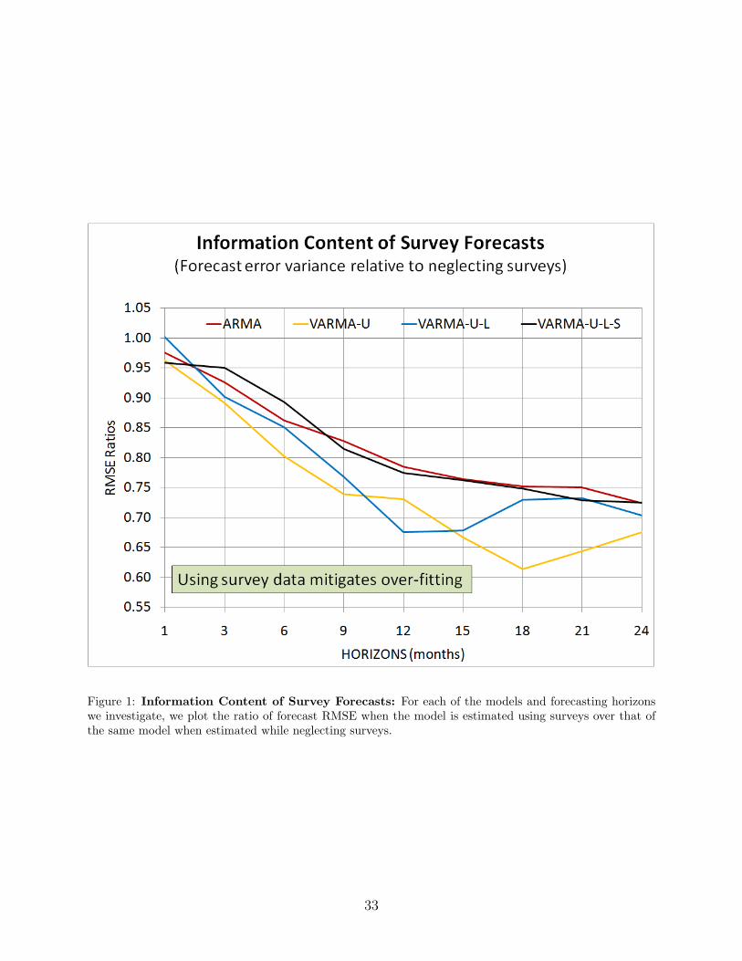
Figure 1: Information Content of Survey Forecasts: For each of the models and forecasting horizonswe investigate, we plot the ratio of forecast RMSE when the model is estimated using surveys over that ofthe same model when estimated while neglecting surveys.

33

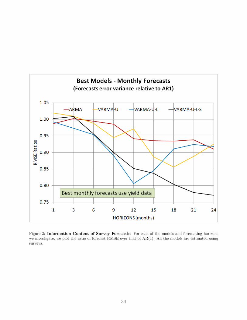
Figure 2: Information Content of Survey Forecasts: For each of the models and forecasting horizonswe investigate, we plot the ratio of forecast RMSE over that of AR(1). All the models are estimated usingsurveys.

34

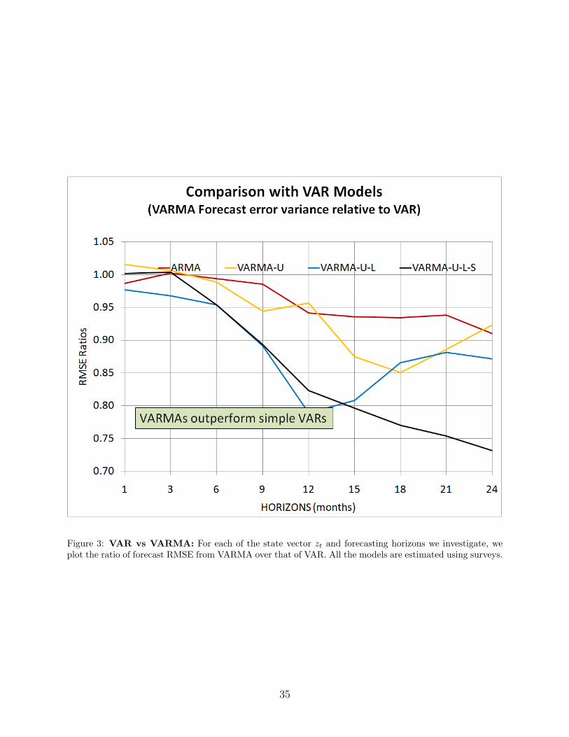
Figure 3: VAR vs VARMA: For each of the state vector zt and forecasting horizons we investigate, weplot the ratio of forecast RMSE from VARMA over that of VAR. All the models are estimated using surveys.

35

Figure 4: Comparison with Surveys: For each of the models and forecasting horizons we investigate, weplot the ratio of forecast RMSE over that of surveys. All the models are estimated using surveys. Becausesurveys data are available only quarterly, all the forecast errors are sampled quarterly prior to computingthe RMSEs.

36

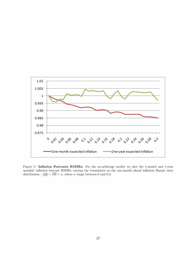
Figure 5: Inflation Forecasts RMSEs: For the no-arbitrage model, we plot the 1-month and 1-yearmonthly inflation forecast RMSEs varying the boundaries on the one-month ahead inflation Sharpe ratiodistribution −SR = SR = κ, where κ range between 0 and 0.3.

37

Q2−

92Q

2−96

Q2−

00Q

2−04

Q2−

08−

1

−0.

50

0.51

1.52

2.53

3.54

1 qu

arte

r

Q3−

92Q

3−96

Q3−

00Q

3−04

Q3−

08−

0.50

0.51

1.52

2.53

3.54

2 qu

arte

rs

Q1−

93Q

1−97

Q1−

01Q

1−05

Q1−

09−

0.50

0.51

1.52

2.53

3.54

3 qu

arte

rs

Q2−

93Q

2−97

Q2−

01Q

2−05

Q2−

09−

0.50

0.51

1.52

2.53

3.5

4 qu

arte

rs

Rea

lized

Our

Mod

elS

PF

Rea

lized

Our

Mod

elS

PF

Rea

lized

Our

Mod

elS

PF

Rea

lized

Our

Mod

elS

PF

Figure

6:In

flation

and

Inflation

Expecta

tions:

WeplottheQuarterlyinflation,survey

forecastsan

dno-arbitrage

model-implied

inflation

expectation

s,from

Q1-19

92to

Q2-20

12,at

horizon

sof

1,2,

3an

d4quarters

ahead.

38

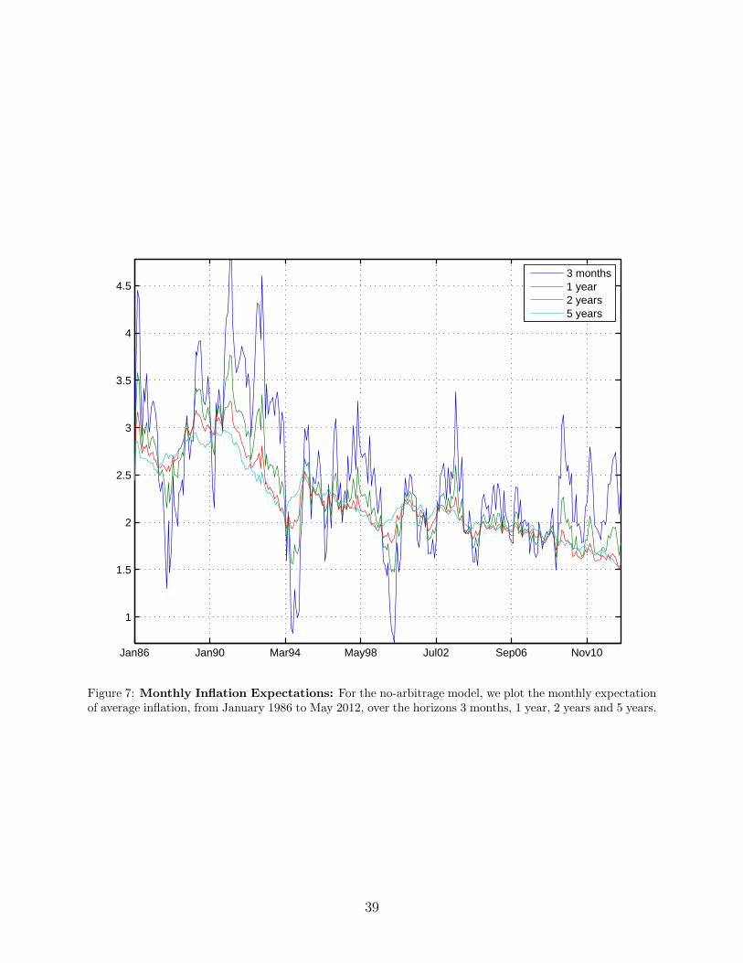
Jan86 Jan90 Mar94 May98 Jul02 Sep06 Nov10

1

1.5

2

2.5

3

3.5

4

4.5

3 months1 year2 years5 years

Figure 7: Monthly Inflation Expectations: For the no-arbitrage model, we plot the monthly expectationof average inflation, from January 1986 to May 2012, over the horizons 3 months, 1 year, 2 years and 5 years.

39

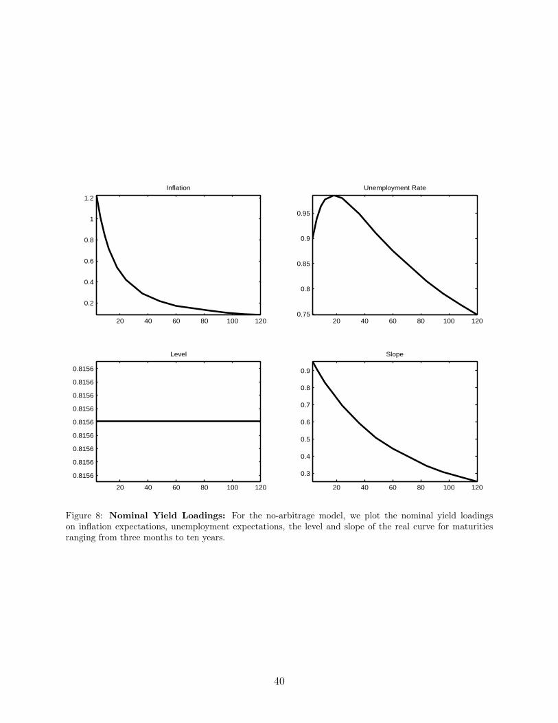
20 40 60 80 100 120

0.2

0.4

0.6

0.8

1

1.2

Inflation

20 40 60 80 100 1200.75

0.8

0.85

0.9

0.95

Unemployment Rate

20 40 60 80 100 120

0.8156

0.8156

0.8156

0.8156

0.8156

0.8156

0.8156

0.8156

0.8156

Level

20 40 60 80 100 120

0.3

0.4

0.5

0.6

0.7

0.8

0.9

Slope

Figure 8: Nominal Yield Loadings: For the no-arbitrage model, we plot the nominal yield loadingson inflation expectations, unemployment expectations, the level and slope of the real curve for maturitiesranging from three months to ten years.

40

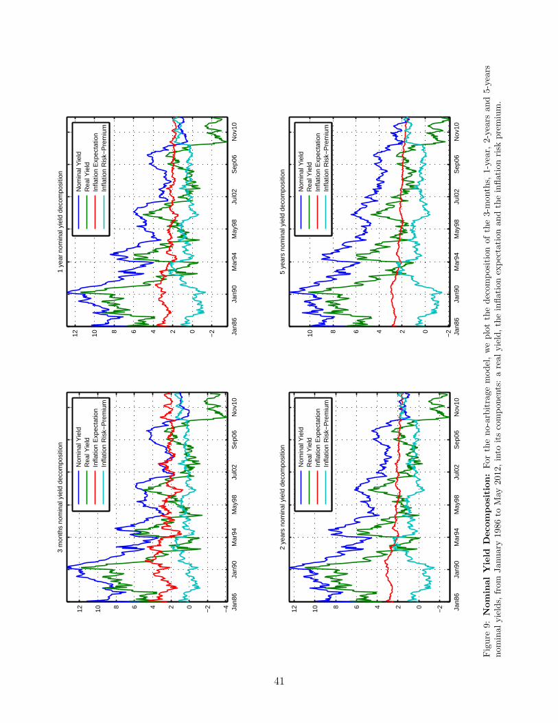
Jan8

6Ja

n90

Mar

94M

ay98

Jul0

2S

ep06

Nov

10−

4

−2024681012

3 m

onth

s no

min

al y

ield

dec

ompo

sitio

n

Jan8

6Ja

n90

Mar

94M

ay98

Jul0

2S

ep06

Nov

10

−2024681012

1 ye

ar n

omin

al y

ield

dec

ompo

sitio

n

Jan8

6Ja

n90

Mar

94M

ay98

Jul0

2S

ep06

Nov

10

−2024681012

2 ye

ars

nom

inal

yie

ld d

ecom

posi

tion

Jan8

6Ja

n90

Mar

94M

ay98

Jul0

2S

ep06

Nov

10−

20246810

5 ye

ars

nom

inal

yie

ld d

ecom

posi

tion

Nom

inal

Yie

ldR

eal Y

ield

Infla

tion

Exp

ecta

tion

Infla

tion

Ris

k−P

rem

ium

Nom

inal

Yie

ldR

eal Y

ield

Infla

tion

Exp

ecta

tion

Infla

tion

Ris

k−P

rem

ium

Nom

inal

Yie

ldR

eal Y

ield

Infla

tion

Exp

ecta

tion

Infla

tion

Ris

k−P

rem

ium

Nom

inal

Yie

ldR

eal Y

ield

Infla

tion

Exp

ecta

tion

Infla

tion

Ris

k−P

rem

ium

Figure

9:NominalYield

Decomposition:For

theno-arbitrage

model,weplotthedecom

positionof

the3-mon

ths,

1-year,

2-years

and5-years

nom

inal

yields,

from

Jan

uary19

86to

May

2012

,into

itscompon

ents:areal

yield,theinflationexpectation

andtheinflationrisk

premium.

41

Figure

10:Contribution

toth

e2-yrIn

flation

RiskPre

mium:For

theno-arbitrage

model,weplotcontribution

ofexpectedinflation,expected

unem

ploymentrate

andoftheexpectedlevel

andslop

efactors,

tothevariationsof

the2-yrinflationrisk

premium.

42

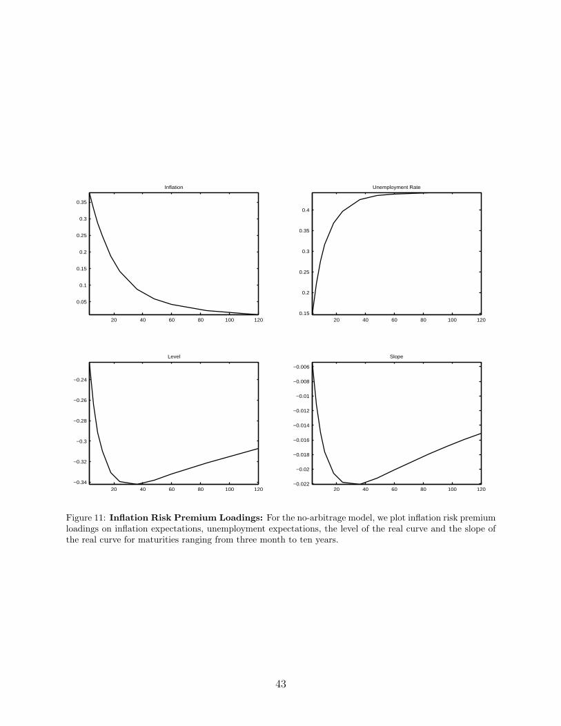
20 40 60 80 100 120

0.05

0.1

0.15

0.2

0.25

0.3

0.35

Inflation

20 40 60 80 100 1200.15

0.2

0.25

0.3

0.35

0.4

Unemployment Rate

20 40 60 80 100 120−0.34

−0.32

−0.3

−0.28

−0.26

−0.24

Level

20 40 60 80 100 120−0.022

−0.02

−0.018

−0.016

−0.014

−0.012

−0.01

−0.008

−0.006

Slope

Figure 11: Inflation Risk Premium Loadings: For the no-arbitrage model, we plot inflation risk premiumloadings on inflation expectations, unemployment expectations, the level of the real curve and the slope ofthe real curve for maturities ranging from three month to ten years.

43

(A) - Components of Unemployment Loadings

(B) - Components of Level Loadings

Figure 12: Sources of Inflation Risk Premium:

For the no-arbitrage model, Panel 12A draws the four components of the loadings of expectedunemployment on the 2-year inflation risk premium. Panel 12B draws the four componentsof the loadings of the level factor on the 2-year inflation risk premium. Horizons up to 60months.

44

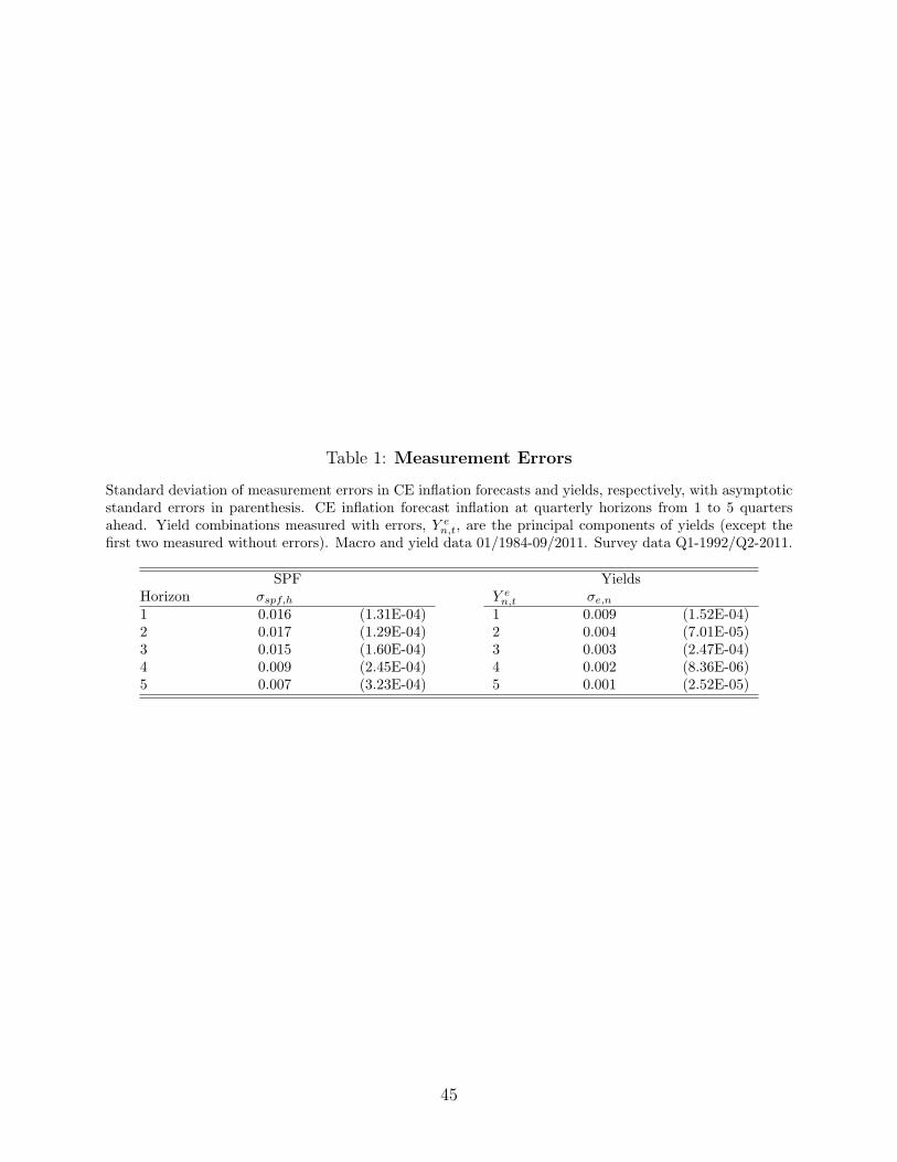
Table 1: Measurement Errors

Standard deviation of measurement errors in CE inflation forecasts and yields, respectively, with asymptoticstandard errors in parenthesis. CE inflation forecast inflation at quarterly horizons from 1 to 5 quartersahead. Yield combinations measured with errors, Y e

n,t, are the principal components of yields (except thefirst two measured without errors). Macro and yield data 01/1984-09/2011. Survey data Q1-1992/Q2-2011.

SPF YieldsHorizon σspf,h Y e

n,t σe,n1 0.016 (1.31E-04) 1 0.009 (1.52E-04)2 0.017 (1.29E-04) 2 0.004 (7.01E-05)3 0.015 (1.60E-04) 3 0.003 (2.47E-04)4 0.009 (2.45E-04) 4 0.002 (8.36E-06)5 0.007 (3.23E-04) 5 0.001 (2.52E-05)

45

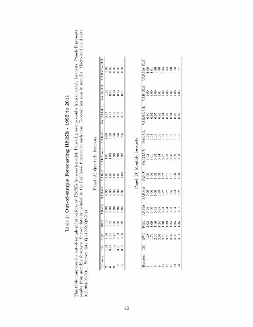
Tab

le2:

Out-of-sample

Foreca

stingRM

SE

-1992to

2011

Thistablecompares

theout-of-sampleinflationforecast

RMSEsfrom

each

model.Pan

elA

presents

resultsfrom

quarterlyforecasts.

Pan

elsBpresents

resultsfrom

mon

thly

forecasts.

Survey

data

isincluded

inthelikelihoodfunctionin

each

case.Forecasthorizon

sin

mon

ths.

Macro

andyield

data

01/1

984-09

/201

1.Survey

data

Q1-199

2/Q2-20

11.

Pan

el(A

)Quarterlyforecasts

Horizo

nCE

RW

1RW

2ARMA

SARMA

VAR-U

VARMA-U

VAR-U

LVARMA-U

LVAR-U

LS

VARMA-U

LS

31.01

1.96

1.13

0.99

0.95

1.01

1.01

1.00

0.97

1.00

1.01

60.95

2.81

1.22

0.99

0.90

1.01

1.00

0.99

0.95

0.99

0.98

91.02

3.71

1.31

0.96

0.95

1.01

0.98

0.96

0.89

0.97

0.95

12

0.93

4.03

1.34

0.96

0.96

1.01

0.96

0.96

0.89

0.97

0.92

15

0.92

3.80

1.21

0.95

0.94

1.00

0.92

0.96

0.92

0.95

0.94

Pan

el(B

)Mon

thly

forecasts

Horizo

nCE

RW

1RW

2ARMA

SARMA

VAR-U

VARMA-U

VAR-U

LVARMA-U

LVAR-U

LS

VARMA-U

LS

11.28

1.02

0.99

0.99

1.00

1.02

1.02

0.99

1.00

1.00

31.74

1.09

1.00

1.00

1.00

1.01

1.01

0.97

1.00

1.01

62.36

1.16

0.99

1.00

1.00

0.99

1.00

0.95

1.00

0.96

92.97

1.24

0.99

0.99

1.00

0.94

1.00

0.89

1.01

0.90

12

3.20

1.30

0.94

0.97

1.02

0.97

1.02

0.81

1.03

0.85

15

3.70

1.33

0.94

0.97

1.01

0.89

1.05

0.84

1.05

0.84

18

3.87

1.34

0.93

0.95

1.01

0.86

1.05

0.91

1.04

0.80

21

4.06

1.35

0.94

0.94

1.00

0.89

1.05

0.92

1.03

0.78

24

4.11

1.35

0.91

0.92

1.00

0.93

1.05

0.92

1.05

0.77

46

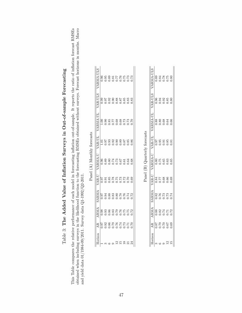
Tab

le3:

TheAddedValueofIn

flation

Surv

eysin

Out-of-sample

Foreca

sting

This

Table

compares

therelativeperform

ance

ofeach

model

inforecastinginflationou

t-of-sam

ple.It

reports

theratioof

inflationforecast

RMSEs

obtained

when

includingsurveysin

thelikelihoodfunctionto

theforecastingRMSEsob

tained

withou

tsurveys.

Forecasthorizon

sin

months.

Macro

andyield

data01

/198

4-09

/201

1.Survey

dataQ1-19

92/Q

2-20

11.

Pan

el(A

)Mon

thly

forecasts

Horizo

nAR

ARMA

SARMA

VAR-U

VARMA-U

VAR-U

LVARMA-U

LVAR-U

LS

VARMA-U

LS

10.97

0.98

0.97

0.97

0.96

1.01

1.00

0.99

0.96

30.92

0.93

0.94

0.91

0.89

0.97

0.90

0.97

0.95

60.86

0.86

0.88

0.85

0.80

0.93

0.85

0.92

0.89

90.79

0.83

0.83

0.78

0.74

0.92

0.77

0.90

0.81

12

0.76

0.79

0.80

0.75

0.73

0.90

0.68

0.88

0.77

15

0.74

0.76

0.78

0.73

0.67

0.89

0.68

0.87

0.76

18

0.73

0.75

0.76

0.72

0.61

0.87

0.73

0.85

0.75

21

0.71

0.75

0.74

0.70

0.64

0.85

0.73

0.83

0.73

24

0.70

0.72

0.72

0.69

0.68

0.86

0.70

0.83

0.73

Pan

el(B

)Quarterlyforecasts

Horizo

nAR

ARMA

SARMA

VAR-U

VARMA-U

VAR-U

LVARMA-U

LVAR-U

LS

VARMA-U

LS

30.87

0.88

0.82

0.84

0.80

0.97

0.88

0.96

0.89

60.79

0.82

0.76

0.77

0.75

0.95

0.80

0.94

0.84

90.70

0.74

0.73

0.68

0.65

0.91

0.68

0.92

0.78

12

0.67

0.71

0.73

0.66

0.63

0.85

0.64

0.85

0.75

15

0.69

0.72

0.74

0.69

0.65

0.81

0.66

0.80

0.80

47

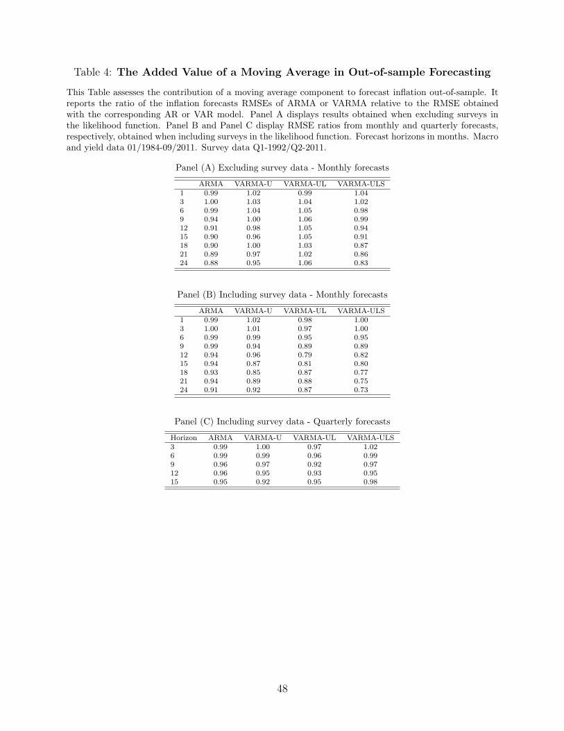
Table 4: The Added Value of a Moving Average in Out-of-sample Forecasting

This Table assesses the contribution of a moving average component to forecast inflation out-of-sample. Itreports the ratio of the inflation forecasts RMSEs of ARMA or VARMA relative to the RMSE obtainedwith the corresponding AR or VAR model. Panel A displays results obtained when excluding surveys inthe likelihood function. Panel B and Panel C display RMSE ratios from monthly and quarterly forecasts,respectively, obtained when including surveys in the likelihood function. Forecast horizons in months. Macroand yield data 01/1984-09/2011. Survey data Q1-1992/Q2-2011.

Panel (A) Excluding survey data - Monthly forecasts

ARMA VARMA-U VARMA-UL VARMA-ULS1 0.99 1.02 0.99 1.043 1.00 1.03 1.04 1.026 0.99 1.04 1.05 0.989 0.94 1.00 1.06 0.9912 0.91 0.98 1.05 0.9415 0.90 0.96 1.05 0.9118 0.90 1.00 1.03 0.8721 0.89 0.97 1.02 0.8624 0.88 0.95 1.06 0.83

Panel (B) Including survey data - Monthly forecasts

ARMA VARMA-U VARMA-UL VARMA-ULS1 0.99 1.02 0.98 1.003 1.00 1.01 0.97 1.006 0.99 0.99 0.95 0.959 0.99 0.94 0.89 0.8912 0.94 0.96 0.79 0.8215 0.94 0.87 0.81 0.8018 0.93 0.85 0.87 0.7721 0.94 0.89 0.88 0.7524 0.91 0.92 0.87 0.73

Panel (C) Including survey data - Quarterly forecasts

Horizon ARMA VARMA-U VARMA-UL VARMA-ULS3 0.99 1.00 0.97 1.026 0.99 0.99 0.96 0.999 0.96 0.97 0.92 0.9712 0.96 0.95 0.93 0.9515 0.95 0.92 0.95 0.98

48

Tab

le5:

CanM

odelForeca

stsIm

provesSurv

eyForeca

st?

This

Table

compares

theperform

ance

ofeach

model’s

RMSE

withsurvey

forecast

RMSEs.

Itreports

theratioof

theinflationforecast

RMSEs

relativeto

theRMSEsfrom

survey

forecasts.

Survey

datais

included

atestimationin

allcases.

Forecasthorizon

sin

mon

ths.

Macro

andyield

data

01/1

984-09

/201

1.Survey

data

Q1-199

2/Q2-20

11.

AR

ARMA

SARMA

VAR-U

VARMA-U

VAR-U

LVARMA-U

LVAR-U

LS

VARMA-U

LS

30.99

0.98

0.95

1.00

1.00

0.99

0.96

0.99

1.00

61.05

1.04

0.95

1.06

1.05

1.04

1.00

1.04

1.03

90.98

0.95

0.93

0.99

0.96

0.94

0.87

0.95

0.93

12

1.08

1.03

1.03

1.09

1.04

1.04

0.97

1.05

0.99

15

1.09

1.04

1.03

1.09

1.01

1.05

1.00

1.04

1.02

49

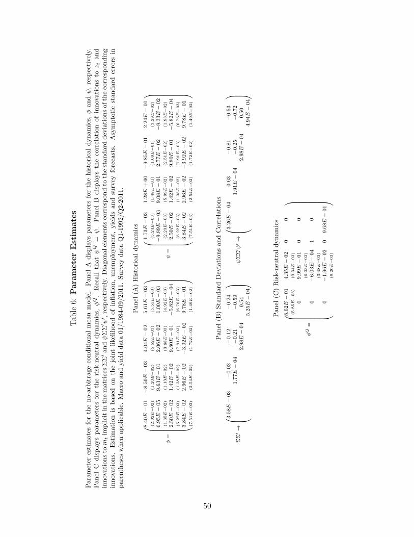
Tab

le6:

Para

meterEstim

ates

Param

eter

estimates

fortheno-arbitrageconditional

meanmodel.Pan

elA

displaysparam

etersforthehistoricaldynam

ics,ϕan

dψ,respectively.

Pan

elC

displaysparam

etersfortherisk-neu

tral

dynam

ics,ϕQ.

Recallthat

ψQ

=ψ.

Pan

elB

displaysthecorrelationof

innovationsto

z tand

innovationstom

tim

plicitin

thematricesΣΣ

′an

dψΣΣ

′ ψ′ ,respectively.

Diago

nal

elem

ents

correspon

dto

thestan

darddeviation

sof

thecorresponding

innovations.

Estim

ationis

based

onthejointlikelihoodof

inflation,unem

ployment,

yieldsan

dsurvey

forecasts.

Asymptoticstan

dard

errors

inparentheses

when

applicable.Macroan

dyield

data01

/198

4-09

/201

1.Survey

dataQ1-19

92/Q

2-20

11.

Pan

el(A

)Historicaldynam

ics

ϕ=

8.40E

−01

−8.50E

−03

4.04E

−02

5.61E

−03

(2.02E−02)

(1.20E−02)

(5.52E−03)

(5.55E−03)

6.95E

−05

9.63E

−01

2.06E

−02

1.00E

−03

(1.35E−02)

(1.13E−02)

(3.68E−03)

(4.92E−03)

2.50E

−02

1.42E

−02

9.80E

−01

−5.82E

−04

(5.22E−03)

(1.38E−02)

(7.91E−03)

(6.76E−03)

3.84E

−02

2.96E

−02

−3.92E

−02

9.78E

−01

(7.51E−03)

(2.54E−02)

(1.72E−02)

(1.49E−02)

ψ

=

1.73E

−03

1.28E

+00

−9.85E

−01

2.24E

−01

(5.24E−03)

(1.48E−01)

(1.00E−01)

(3.29E−02)

−9.89E

−03

9.08E

−01

2.77E

−02

−8.33E

−02

(2.23E−03)

(5.99E−02)

(2.51E−02)

(1.93E−02)

2.50E

−02

1.42E

−02

9.80E

−01

−5.82E

−04

(5.22E−03)

(1.38E−02)

(7.91E−03)

(6.76E−03)

3.84E

−02

2.96E

−02

−3.92E

−02

9.78E

−01

(7.51E−03)

(2.54E−02)

(1.72E−02)

(1.49E−02)

Pan

el(B

)StandardDeviation

san

dCorrelation

s

ΣΣ

′→

3.58E

−03

−0.03

−0.12

−0.24

1.77E

−04

−0.21

−0.59

2.98E

−04

0.54

5.25E

−04

ψΣΣ

′ ψ′→

3.26E

−04

0.63

−0.81

−0.53

1.91E

−04

−0.25

−0.72

2.98E

−04

0.50

4.94E

−04

Pan

el(C

)Risk-neu

tral

dynam

ics

ϕQ

=

8.62E

−01

4.35E

−02

00

(5.85E−03)

(9.34E−03)

09.99E

−01

00

(6.03E−03)

0−6.03E

−04

10

(3.48E−03)

0−1.96E

−02

09.68E

−01

(8.20E−03)

50

Table 7: Model Implied Summary Statistics

Sample summary statistics of nominal yields, y(n)t , real yields, i

(n)t , and inflation risk premium, rpπt,n, at

different maturities, n, as well as inflation expectation, mπt,h, at the corresponding horizons, h. These quan-

tities are computed from the no-arbitrage model estimated using the state variables, CE inflation forecastsand yields, jointly. Macro and yield data 01/1984-09/2011. Survey data Q1-1992/Q2-2011.

3 months 6months

y(n)t i

(n)t mπ

t,h rpπt,n y(n)t i

(n)t mπ

t,h rpπt,nMean 5.06 2.15 2.47 0.44 5.12 2.22 2.39 0.51Median 4.57 1.67 2.36 0.40 4.67 1.68 2.25 0.48Std 3.27 3.35 0.74 0.58 3.17 3.29 0.62 0.66AC(1) 0.99 0.98 0.90 0.92 0.99 0.98 0.92 0.93AC(3) 0.97 0.94 0.76 0.77 0.97 0.94 0.80 0.81AC(6) 0.94 0.87 0.56 0.58 0.94 0.88 0.65 0.65AC(12) 0.86 0.76 0.33 0.33 0.87 0.76 0.46 0.42

1 year 2 year

y(n)t i

(n)t mπ

t,h rpπt,n y(n)t i

(n)t mπ

t,h rpπt,nMean 5.23 2.35 2.29 0.58 5.44 2.57 2.22 0.62Median 4.71 1.71 2.15 0.54 4.9 1.91 2.12 0.56Std 3.03 3.17 0.51 0.76 2.84 2.99 0.44 0.83AC(1) 0.99 0.98 0.96 0.95 0.99 0.98 0.99 0.96AC(3) 0.97 0.94 0.89 0.86 0.97 0.94 0.97 0.89AC(6) 0.94 0.88 0.81 0.72 0.94 0.89 0.94 0.78AC(12) 0.88 0.77 0.68 0.51 0.9 0.79 0.87 0.58

3 years 5years

y(n)t i

(n)t mπ

t,h rpπt,n y(n)t i

(n)t mπ

t,h rpπt,nMean 5.61 2.75 2.21 0.61 5.89 3.04 2.21 0.57Median 5.07 2.09 2.12 0.56 5.43 2.38 2.15 0.53Std 2.71 2.85 0.41 0.84 2.56 2.67 0.37 0.82AC(1) 0.99 0.98 0.99 0.97 0.99 0.98 0.99 0.97AC(3) 0.97 0.95 0.98 0.91 0.97 0.95 0.99 0.92AC(6) 0.95 0.89 0.96 0.8 0.95 0.9 0.97 0.82AC(12) 0.91 0.81 0.91 0.61 0.92 0.83 0.93 0.63

51