Forecasting Exchange Rates: An Investor Perspective

Michael Melvin John Prins

Duncan Shand

CESIFO WORKING PAPER NO. 4238 CATEGORY 7: MONETARY POLICY AND INTERNATIONAL FINANCE

MAY 2013

An electronic version of the paper may be downloaded • from the SSRN website: www.SSRN.com • from the RePEc website: www.RePEc.org

• from the CESifo website: Twww.CESifo-group.org/wp T

CESifo Working Paper No. 4238

Forecasting Exchange Rates: An Investor Perspective

Abstract The popular scholarly exercise of evaluating exchange rate forecasting models relative to a random walk was stimulated by the well-cited Meese and Rogoff (1983) paper. Practitioners who construct quantitative models for trading exchange rates approach forecasting from a different perspective. Rather than focus on forecast errors for bilateral exchange rates, as in the Meese-Rogoff case, we present what is required for constructing a successful trading model. To provide more perspective, a particular approach to quantitative modeling is presented that incorporates return forecasts, a risk model, and a transaction cost constraint in an optimization framework. Since beating a random walk is not a useful evaluation metric for currency investing, we discuss the use of benchmarks and conclude that performance evaluation in currencies is much more problematic than in equity markets due to the lack of a passive investment strategy and the multitude of alternative formulations of well-known currency style factors. We then provide analytical tools that can be useful in evaluating currency manager skill in terms of portfolio tilts and timing. Finally, we examine how conditioning information can be employed to enhance timing skill in trading generic styles like the carry trade. Such information can be valuable in reducing the duration and magnitude of portfolio drawdowns.

JEL-Code: C520, C530, C580, F310, F370, G150, G170.

Keywords: exchange rate forecasting, forecast evaluation, conditioners, quantitative models, benchmarks.

Michael Melvin

BlackRock San Francisco / USA michael.melvin@blackrock.com

John Prins BlackRock San Francisco / USA

john.prins@blackrock.com

Duncan Shand BlackRock London / United Kingdom

duncan.shand@blackrock.com Forthcoming in Elliott and Timmermann Handbook of Economic Forecasting; Vol 2; Elsevier.

1

1. Introduction

Exchange rate forecasting consumes a vast amount of space in the scholarly literature of

international finance. Summaries of this large literature have been provided from time to

time by several authors1 but the focus has generally been on finding models that can

forecast the future spot exchange rate better than a random walk. The well-cited paper by

Meese and Rogoff (1983) spawned a leap in research attention as scholars attempted to

take up the challenge of developing new models to beat a random walk for exchange

rates. It is not clear that we have learned much since the 1980s other than it is still quite

challenging to construct a model that is capable of systematically outperforming a

random walk in predicting future spot exchange rates. This academic focus on predicting

bilateral exchange rates is understandable and certainly a subject worthy of scholarly

attention, however the exercise undertaken by scholars is pursuing answers to questions

that are not necessary for successful investing in currency markets. This chapter aims to

lay out key issues of exchange rate forecasting from a quantitative practitioner’s

perspective. By the end of the chapter, the reader should have answers to the following

questions:

1. Why don’t we need accurate forecasts of future spot exchange rates to construct

currency portfolios that yield attractive returns?

Section 2 addresses the irrelevance of the Meese-Rogoff exchange rate disconnect puzzle

for currency investors. Of course, Meese and Rogoff were focused on testing popular

exchange rate models from an academic perspective and not creating investment

portfolios. One way of viewing the difference is in terms of different loss functions. The

academic exercise uses a measure like mean square forecasting error, while the active

currency investor focuses on a measure like a Sharpe ratio or risk-adjusted returns. We

will give a clear example of the difference that results from the two perspectives.2

2. How does one go about constructing an actively managed currency portfolio?

Section 3 provides a high-level overview of the elements of building actively-managed

quantitative currency portfolios as a currency hedge fund manager might use. While

currency return forecasts are key, one needs more than just return forecasts to put

together a successful long-short model.

3. How should currency portfolio managers be evaluated?

A simple answer is whether they generate attractive risk-adjusted returns or not. But is

there such a concept as “beta” in currency investing, as exists in equity investing? In

other words, is there a passive investment style benchmark against which one can judge

1 Papers giving a good overview of this vast literature include Frankel and Rose (1995), Taylor (1995);

Sarno and Taylor (2002); Cheung, Chinn, and Pascual (2005); Engel, Mark, and West (2007); Della Corte,

Sarno, and Tsiakas (2009); Williamson (2009); and Evans (2011) 2 Other authors have considered alternatives to mean square forecast error in evaluating forecasts in other

financial settings. Foreign exchange examples include Elliott and Ito (1999) and Satchell and Timmermann

(1995).

2

performance in currency investing? Section 4 looks into this question and finds that

identifying useful benchmarks for active currency investing is problematic.

4. Lacking good benchmarks for assessing currency portfolio performance, are

there other analytical tools that can be employed to help evaluate portfolio

managers?

Section 5 describes how one can break down portfolio returns to evaluate a manager’s

skill in timing return-generating factors. Portfolio returns are decomposed into tilt and

timing components. The “tilt” in a portfolio refers to holding constant exposures to assets

over time, and is a kind of passive investing. The “timing” component of portfolio

returns is the difference between total returns and the tilt returns. We can see that

different generic currency investing styles offer different tilt versus timing returns.

5. Can one enhance returns by the use of conditioning information to help time

exposures to return-generating factors?

Following on from the timing discussion of Section 5, Section 6 creates a specific

example of the use of conditioning information to enhance returns from the carry trade. A

carry trade involves buying (or being long) high interest rate currencies, while selling (or

being short) low interest rate currencies. By dialing down risk in times of financial

market stress, one can realize substantially higher returns from investing in the carry

trade.

The chapter concludes with a summary in Section 7.

3

2. Successful investing does not require beating a random walk

The inability of macroeconomic models to generate point forecasts of bilateral exchange

rates that are more accurate than forecasts based on the assumption of a random walk,

particularly at horizons shorter than one year, is known as the ‘exchange rate disconnect

puzzle’ (Obstfeld and Rogoff 2001). Since it was first established by Meese and Rogoff

(1983), this puzzle has mostly resisted a quarter century of empirical work attempting to

overturn it, and remains one of the best-known challenges in international finance.

Despite its prominence in academic work, however, this challenge is of little relevance to

investors. The investor’s goal is not to generate accurate forecasts of the future levels of

exchange rates, but simply to generate forecasts of returns to these currencies that are

correctly rank-ordered in the cross-section. It is the ordering of these return forecasts

relative to one another that matters, not their absolute magnitude. An investor’s forecasts

of returns might be substantially worse than those of a random walk, but as long as they

are more or less correctly ordered relative to one another, one can still consistently make

money. In short, successful investing does not require beating a random walk.

To illustrate the difference between the approaches of the typical academic and

practitioner, consider the following simple example. Suppose the investor has three

currencies in his tradeable universe: dollar, euro and yen. EURUSD today is trading at

1.50 and USDJPY is trading at 100. He forecasts the Yen to depreciate by 10% (leaving

USDJPY at 111) and the Euro to appreciate by 10% (leaving EURUSD at 1.65). He

therefore takes a long position of +50% Euro and an offsetting short position of -50%

Yen in his portfolio, while remaining neutral on the dollar3. Subsequently, EURUSD

ends the period at 1.4850 (a depreciation of 1%) and USDJPY ends the period at 105 (a

depreciation of 5%). The root mean squared error of the investor’s forecasts ( sqrt(((111-

105)/105)^2 + (1.65-1.4850)/1.4850))^2) = 12.5%), is much larger than the root mean

squared error of a forecast based on the random walk ( sqrt(((100-105)/105)^2 + (1.50-

1.4850)/1.4850))^2) = 4.8%). The investor has made two serious mistakes: the magnitude

of his forecasts was totally wrong, expecting moves of 10% in either direction when only

moves of 1% and 5% were realized, and he did not even predict one of the two directions

of change correctly. Nonetheless, despite large errors in his forecasts in regards to both

direction and magnitude, his portfolio made a 2% positive return. This is simply because

his rank ordering of returns for the currencies in which he took active positions (i.e. EUR

> JPY) was correct.

This example demonstrates one of the advantages which the investor has over the

academic. Theory often suggests which fundamental macroeconomic variables should be

relevant to exchange rate determination while remaining silent on the size of the

3 There are many other portfolios the investor could have formed that are consistent with the forecasts of

relative returns that he generated. In practice, the level of risk the investor desires, and his determination of

the optimal hedging portfolio for each position, will determine the exact composition of the portfolio. Here

we choose a simple portfolio for illustrative purposes, with no hedging through the third currency (the

dollar).

4

relationship (ie the true coefficient in a regression of the exchange rate on the

fundamental in question). Thus, for the researcher attempting to produce an accurate

forecast of an exchange rate’s future level, it is necessary to empirically estimate the

relationship which existed historically between the exchange rate and the fundamental,

and use these historical estimates to inform his forecasts. This entails all sorts of

difficulties, including the problems of estimation error in short samples and the

possibility of structural breaks. But as long as the same relationship, whatever it is, holds

across currencies, the investor does not have to worry about these estimation issues. It is

sufficient to rank the currencies in his investible universe according to the fundamental in

question (in level or change space, whichever is more appropriate), and form his long-

short portfolio accordingly4.

The second advantage of the investor is breadth. The Fundamental Law of Active

Management (Grinold and Kahn, 2000) says that a portfolio of 17 currencies (i.e. 16

exchange rates), formed on the basis of forecasts with equal ex-ante skill across

currencies, will have a information ratio5 four times higher than that of a portfolio

consisting of only 2 currencies (i.e., a single exchange rate). Many academic studies,

following Mark and Sul (2001), have also recognized the benefits of breadth and made

use of panel forecasts to overcome the problems of estimating relationships in short

samples, with moderate success at very long horizons. Nonetheless, in terms of

evaluating the success of their forecasts, the majority of the attention has remained fixed

on bilateral exchange rates,6 whereas the investor’s success is measured across the

realized cross-section of returns.

The rest of this section develops a real example of a fundamental we might expect to

have relevance to forecasting exchange rates, and evaluates it against the academic’s and

investor’s benchmarks, showing that while it has only very limited success in the

academic context, it fares better as an investment strategy. Consider the concept of

purchasing power parity, which states that the same tradeable good should sell for the

same price in different currencies. For non-tradable goods, between countries with very

different levels of productivity in their tradable sectors, this law certainly need not hold

(Dornbusch, 1979) - think of the difference in price between a haircut in India and

Switzerland. But it is a reasonable working hypothesis for countries at roughly the same

4 If the investor wishes to use more than one fundamental to rank currencies, a difficulty can arise if two

factors are highly correlated and have opposite signs. Then it becomes necessary to know the relative

magnitudes of the two effects. To circumvent this difficulty in practice, investors simply try to make sure

the fundamentals they use as the building blocks of their portfolios are fairly independent. 5 The information ratio (IR) is the expected active return (the return in excess of a passive benchmark

return) divided by the standard deviation of the active return. Section 5 provides some examples generating

IR values, while Section 4 discusses the challenges of identifying useful benchmark portfolios for active

currency investing. 6 For an example of a recent paper which uses panel estimation techniques, but still evaluates forecast

accuracy against each bilateral exchange rate independently, see Molodtsova and Papell (2009). For

examples of recent papers which do evaluate the success of strategies in a portfolio setting, see Burnside,

Eichenbaum, Kleshchelski and Rebelo (2006), Lustig and Verdelhan (2007), Ang and Chen (2010) and

Lustig, Roussanov and Verdelhan (2011).

5

level of economic development, and low barriers to trade and technological diffusion,

that if a country’s currency deviates significantly from purchasing power parity with its

peers, we might expect it to revert. Using data on relative price levels between countries,

together with current spot exchange rates, we can therefore construct forecasts for each

currency at each point in time based on the hypothesis of reversion to PPP, and test our

model both in an academic and a portfolio setting.

In terms of data, we proceed as follows. In its biannual World Economic Outlook reports,

the International Monetary Fund publishes estimates of purchasing power parity based on

sporadic surveys conducted by the International Comparison Program (ICP), a division of

the World Bank. At each point in time, we take the latest estimate of purchasing power

parity available at the time as our estimate of the currency’s fair value. Then, the

deviation of the current spot price from this fair value, in percentage terms, is our forecast

of the expected change in the spot price. To be precise, if the spot price is defined in

terms of units of the currency per US dollar, then a spot price higher than the fair value

determined by the IMF’s estimates of purchasing power parity indicates that the currency

is weaker than fair value, and we therefore forecast for this currency a positive return.

We use the exchange rates of the eight developed countries which have been

continuously in existence since 1980 when the IMF’s PPP data first becomes available:

the British Pound, the Japanese Yen, the Swiss Franc, the Canadian Dollar, the Australian

Dollar, the New Zealand Dollar, the Swedish Krona and the Norwegian Krone. For the

purposes of this exercise, we omit the Euro and its forebears as they have only been in

existence for (mutually exclusive) parts of the sample. In each month, the value of PPP

that we use is that which was published in the previous year’s October WEO report. The

value of spot that we use is the London 4pm WM fixing price7 from two days prior to the

beginning of the month. The use of PPP estimated from the previous year, and spot data

from the previous month, ensures that the data we use in our forecast were available at

the time the forecast was made, and that the forecasts are therefore out-of-sample and the

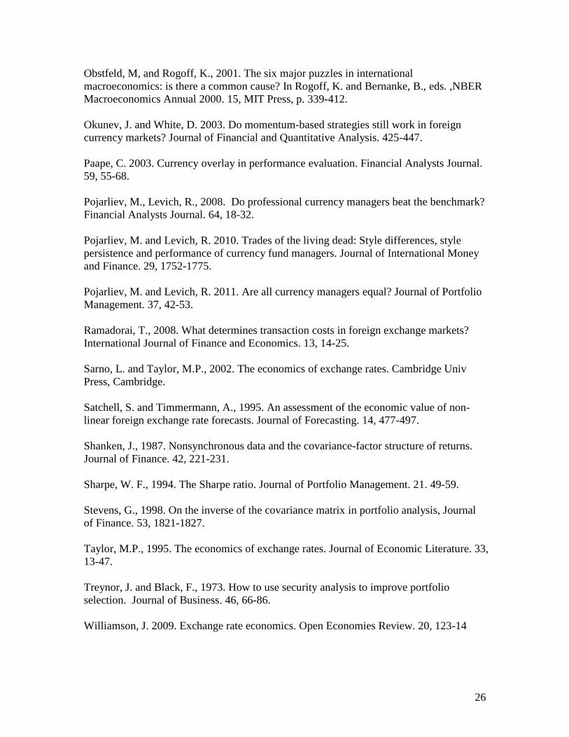
trading strategy based on it is investible. Figure 1 plots the spot exchange rate along with

the PPP-implied fair value for each currency.

We contrast the results of two different approaches to evaluating the relevance of these

forecasts to exchange rates: the academic approach of whether we can reject the null

hypothesis that each exchange rate follows a random walk, and the practitioner’s

approach of whether a portfolio formed on the basis of these forecasts has a information

ratio statistically significantly different from zero. For the first approach, we use four

standard tests of out-of-sample predictability applied in the literature: Clark-West, Clark-

McCracken, Diebold-Mariano and Theil’s U. For the second approach, we construct a

long-short portfolio of the currencies in our universe, rebalanced at the beginning of each

month. More details on how such portfolios are typically constructed by quantitative

investors are provided in Section 4. For the purposes of evaluating the performance of the

7 The London 4pm WM fixing price is a benchmark price provided by Reuters (formerly WM Company)

for foreign exchange.

6

long-short portfolio, we compare it to a benchmark portfolio with zero holdings. This is

the portfolio which would be generated (also using the methodology of Section 2) by an

assumption of uncovered interest rate parity, where the expected exchange rate change is

equal to the interest differential so that there is no expectation of gain from currency

speculation. The question of whether this is the most appropriate benchmark for a

currency strategy is discussed in more detail in the next section.

The results are shown in Table 1. In the first approach, for no currency are we able to

reject the null hypothesis of a random walk consistently across all four tests. In fact, we

can reject the null for only one currency (CAD) in one test (Clark-McCracken). The tests

across the whole panel of currencies fare slightly better, with success at rejecting the null

at the 1% significance level for two tests (Clark-West and Clark-McCracken), but again

the results are inconsistent across the four tests. We could interpret this as some evidence

that our forecasts contain information that enables us to predict the future levels of

exchange rates better than a random walk, but only for the panel. By contrast, in the

second approach, the information ratio of the portfolio formed from our forecasts is 0.5.

The statistical significance of this information ratio can be evaluated by noting that the t-

statistic is approximately equal to the information ratio multiplied by the square root of

time in years (Grinold and Kahn, 2000). In this case this yields a t-statistic of 0.5 *

sqrt(30) = 2.7, indicating that the information ratio is statistically significantly different

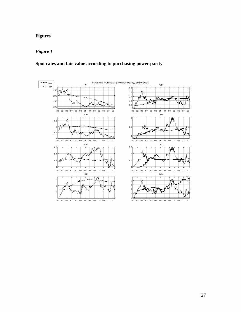
from zero8. A visual inspection of cumulative returns to the portfolio (shown in Figure 2),

normalized to take unit risk, also suggests that performance has been quite consistent

over time.

In summary, the goal of an investor in foreign exchange markets is different to that of

much of the academic literature on forecasting exchange rates. While the gold standard

for academics has been to produce accurate point forecasts for the future levels of

bilateral exchange rates, the investor has an easier task. One only need be concerned with

generating expected returns across a cross-section of currencies which correspond well to

the actual cross-section of realized relative returns. Errors in forecasts can be averaged

out over a large cross-section of currencies, and the rank order of the forecasts matters

more than their size. We showed an example of a fundamental that, while unable to beat a

random walk for any of the individual exchange rates in our sample, generated an

investing strategy which most investors would find fairly attractive. In the sections that

follow, we go into more detail of the investor’s approach: how to construct a portfolio,

how to evaluate this portfolio’s performance, and appropriate benchmarks against which

to measure this performance.

8 Lo (2002) outlines the conditions under which this Grinold and Kahn (2000) result holds, the most

important of which is the absence of serial correlation in returns to the portfolio.

7

3. Constructing a Currency Portfolio

Building a quantitatively modeled active currency portfolio involves 3 key pieces: return

or alpha9 forecasts, a risk model, and a transaction cost model.

10 We can summarize this

with the following utility function to be maximized (over h): ' 'h h Vh TC h ,

where h refers to the portfolio holdings or positions, is the alpha or return forecast,

is the parameter of risk aversion, V is the risk model or, typically, a covariance matrix of

returns, is the transaction cost amortization factor, TC is a transaction cost function,

and h is the change in holdings from last period to this period. A long-short hedge

fund has both positive and negative holdings, so one may also include a sum-to-zero

constraint so that the model is self-funding (the short positions fund the long positions).

We discuss each of these elements of the utility function in turn.

h: the portfolio asset holdings are derived from the utility maximization or

optimization of the portfolio subject to the return forecasts, risk constraint, and

transaction cost model.

: the alpha or return forecast is the key element of the whole enterprise. No matter

how good the risk and transaction cost models, without good forecasts of returns, no

quantitative model can survive. However, what really matters is not the forecast of

actual returns, but the relative ranking of returns across the assets in the fund in order

to identify favored long positions versus shorts. So is aimed at more of an ordinal

ranking than a true expectation.

: the risk aversion parameter is used to scale risk up or down to achieve a target

level of risk. In order to raise (lower) the risk level of the portfolio, we lower (raise)

.

V: is typically a covariance matrix estimated from historical returns. Managers may

apply some Bayesian shrinkage based upon prior information regarding elements of

the matrix. For instance, one may want to force regional blocks to always exist so that

one creates baskets of currencies for hedging that focus on Asia, Europe, and the

Americas to ensure that the returns of currencies in each block are correlated to a

sufficient degree. Alternatively, some managers may blend historical measures of

correlation with forward-looking information as contained in the implied volatility

from option prices.11

: the transaction cost amortization factor controls how much the cost model

intimidates trading. If one wants to penalize the optimization via transaction costs

more, then is raised. If is set to zero, then the model moves to the no-cost

9 Investors often refer to idiosyncratic returns of an asset as “alpha.” This term comes from equity investing

where “beta” is the return that is correlated with the overall market and alpha is the return unique to an

asset. 10

This is not intended to be more than a sketch of model construction techniques. For greater detail on

active portfolio model building see Grinold and Kahn (2000). 11

There are many ways to construct V and there is a fairly large literature associated with the topic. Some

examples of papers in this area that show the variety of approaches include Jorion (1985), Shanken (1987),

Bollerslev, Engle, and Wooldridge (1988), Konno and Yamazaki (1991), Kroner and Ng (1998), Stevens

(1988), Ledoit and Wolf (2004), and Christensen, Kinnebrock, and Podolskij (2010),

8

optimal holdings every day. Typically, this is too much trading and the costs seriously

erode the realized returns. The higher the for given cost forecasts, the slower we

will trade to reach our desired positions. This means that the model will typically

have some backlog as the difference between the zero cost optimal holdings and the

transaction cost intimidated holdings, and this backlog existence is optimal. The

choice of will also depend upon the speed of the factors driving the model holdings.

For a slow model, a relatively high value may be optimal as one would not need to

trade quickly into new positions as the return forecasts are persistent.

TC: the transaction cost function generates estimates of the cost of trading. We can

think of the trade costs as being of two types: a) fixed costs, as in a bid-ask spread

that one must pay; and b) variable costs, as in the market impact of our trades. The

latter arises as our trades may affect the market price. If we are a small fund, then we

will trade small size in all our currencies and market impact is not a concern.

However, if we are a large fund then we will find that the market impact of our trades

may be significant at times and will be increasing in trade size. Costs differ across

currencies, so that we will not have to worry too much about trading euro (EUR)

versus the U.S. dollar (USD), the most liquid market. However, if we trade a less-

liquid currency like the New Zealand dollar (NZD) or Norwegian kroner (NOK)

against the dollar, we will have to be much more careful if we are trading in size.

Table 2 provides information on different transaction costs associated with different

currencies. These are representative spreads a customer would face if calling a bank

and requesting a two-way quote. One can see that costs vary inversely with liquidity

of the currency pair. Trading U.S. dollars against euros at the commonly quoted units

of dollars per euro (EURUSD), has the lowest cost as the most liquid currency pair in

the market. Trading U.S. dollars against New Zealand dollars at the exchange rate

quoted in USD per NZD (NZDUSD), being the least liquid currency pair in the table,

has the highest cost.12

As stated earlier, the most important input into the optimization is the alpha or return

forecast. In the previous section we discussed the importance of getting the ordering of

currencies correct, from the most likely to appreciate to the most likely to depreciate. If

we are unable to forecast this with skill over time, we will not succeed no matter how

good the risk or transaction cost models are. If we have skill, then we will generate alpha

over time. There remains an issue of how an active currency manager should be judged.

Are there benchmarks against which performance can be measured as in equity

investing? The next section takes up this controversial issue.

4. Benchmarks for Currency Investors

Academic forecasting exercises focus on metrics like mean square error when evaluating

alternative forecasts. In the academic literature on forecasting exchange rates, the most

12

There is a limited literature on currency transaction costs. A representative sample of papers includes

Glassman (1987); Bessembinder (1994); Bollerslev and Melvin (1994); Hartmann (1999); Naranjo and

Nimalendran (2000); Melvin and Taylor (2009); and Ramadorai (2007).

9

popular metric is comparing the mean square error of a particular forecast of bilateral

exchange rates against that of a random walk. On the other hand, investors measure

forecast success in terms of model performance in delivering risk-adjusted returns. There

are two broad categories of investing: passive and active. A passive investment strategy

seeks to achieve the same return as some benchmark, like the S&P 500 index of U.S.

equities for passive equity investing. The passive investor holds a portfolio of assets that

will replicate the benchmark return. Active investors seek to outperform a benchmark

return. So active investing in U.S. equities should seek to deliver returns in excess of a

benchmark like the S&P 500. If the active investment strategy cannot outperform the

benchmark, then the investor would be better served by just choosing a lower-cost

passive strategy and not trying to “beat the market.” Foreign exchange markets are

different from other asset classes in some important respects. From an investor’s

perspective, one important difference is the lack of a well-defined benchmark to be used

in assessing investment manager performance. This leads to questions like the following:

How should an active currency manager be evaluated? From the broader perspective,

evaluating the currency forecasts of an active currency manager is more complicated than

in other asset classes due to the lack of an accepted metric for “passive” performance.13

Unlike the equity market, where popular notions of “the market” exist, there is nothing

like that in currencies. One can buy the S&P 500 index and feel reasonably comfortable

that you have a broad exposure to the U.S. equity market. In the foreign exchange market,

one does not “buy and hold.” Since every trade in the foreign exchange market involves

buying one currency while selling another, an investor is naturally long and short across

the chosen currencies. So how may one think about a passive strategy in currencies? First,

there is no such thing as a purely passive strategy. All the various indices that have been

suggested for currency investors involve some degree of active management in that they

must be rebalanced over time as market conditions change. One may conclude that there

really is no passive strategy for currency investors. As a result, trade execution and

strategy are extremely important.

If we rule out the concept of passive investing in the currency market, can we still

identify useful benchmarks for performance evaluation? The suggested benchmarks have

all been indices representing known investment strategies in the currency market: carry,

trend (sometimes called momentum), and value (often some version of purchasing power

parity). Rather than passive strategies, one may think in terms of common risk factors

that currency investors are exposed to. In this spirit, there have been suggestions that

active managers should beat these common factors in order to add value. However, there

are many ways that such strategies are employed by investors and the indices on offer

reflect interesting differences. So the common factors are really not exactly “common.”

For an example, we analyze a representative sample of indices.

13

Papers that address the issue of benchmarks for active currency management include Leqeux and Acar

(1998); Paape (2003); Pojarliev and Levich (2008, 2010, 2011) and Melvin and Shand (2011).

10

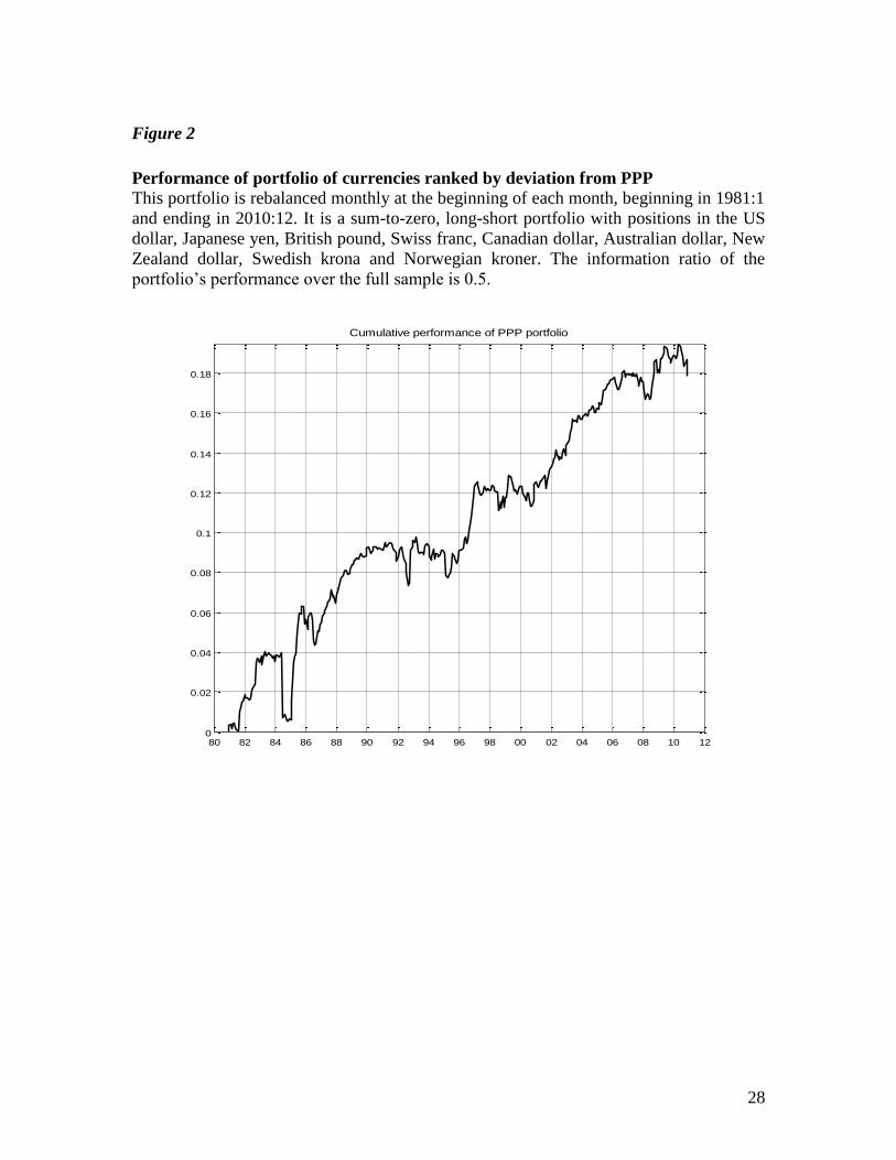
Figure 3 displays cumulative returns from three different trend strategies as offered by

indices created by the Centre for International Banking Economics and Finance (known

as the AFX Currency index), Credit Suisse (CS), and Deutsche Bank (DB). The AFX and

DB samples begin in June 1989, while the CS sample begins in June 1999. A cursory

look at the figure suggests that there is no such thing as a single concept of “trend.” Each

firm has a different approach to modeling exchange rate momentum.

DB calculates 12-month returns and then once-a-month ranks the G10 currencies,

going long the top 3 while shorting the bottom 3.

AFX uses three moving averages of 32, 61, and 117 days and if the current spot

rate exceeds (is less than) a moving average value a long (short) position is

established. The benchmark return is the average of the returns from the three

rules.

CS defines “trend” as a 12-month exponentially-weighted moving average of total

returns (including carry or the interest rate) and then takes long (short) positions

in currencies whose total returns are above (below) the trend. So this trend

concept includes an element of carry.

The cumulative performance of the three different strategies in Figure 4.1 are quite

different at times. One can observe periods when one index is rising while others are flat

or falling. The lesson is that even a simple concept like “trend” can be employed many

different ways which yield differential performance so that it is an oversimplification to

claim that there are clear benchmarks for applying in currency markets. This is reflected

in academic studies of technical analysis in currency markets where survey data indicate

a wide variety of trading rules are employed in trend-following strategies as reported in

the survey by Menkhoff and Taylor (2007).14

To further investigate the extent to which alternative reasonable measures of “benchmark

factors” may differ, we examine correlations across a set of alternative indices as

provided by Deutsche Bank (DB), Credit Suisse (CS), and Citi. For Trend, we also

include the AFX index that was studied by Pojarliev and Levich (2008). Table 3 displays

the estimated correlations. Trend factor index correlations range from 0.20 for AFX/DB

to 0.76 for CS/DB. Carry factor index correlations range from 0.46 for Citi/CS to 0.81 for

Citi/DB. Finally, PPP factor index correlations range from 0.39 for CS/DB to 0.45 for

Citi/DB or Citi/CS. Clearly the notion of a “generic” strategy in currency investing does

not result in alternative indices of the generic factors looking much alike. This is unlike

the case of equity markets where the S&P 500 and the Dow Jones Industrial average have

a correlation of 0.99 over the period from March 1980 to March 2010. In the case of

equities, it is entirely reasonable to talk about the “market” and then benchmark returns

against such a concept. In currency markets, the situation is much different.

14

There is a fairly large literature on so-called technical trading rules for trading currencies, which include

trend-following strategies. A sample of papers includes James (2003); Okunev and White (2003); Neely

and Weller (2009); De Zwart, G., Markwat, T., Swinkels, L., and van Dijk (2009); and Menkhoff, Sarno,

Schmeling, and Schrimpf (forthcoming).

11

Melvin and Shand (2011) analyze a data set of currency hedge fund managers to examine

if the generic investment styles can explain their performance. In other words, were they

just trading the well-known strategies of momentum, trend, and carry, in which case

some might assert that this was just earning “beta” rather than “alpha?” The empirical

results indicate that returns associated with those currency investors are often generated

quite independently from the generic style factors. This seems to be particularly true of

the most successful managers. An analysis of timing ability reveals that some managers

appear to have superior ability to time the factors. Such skill is what investors should

willingly pay for. An additional skill involves risk controls and the analysis indicates that

many managers have ability in avoiding worst-case drawdowns that are associated with a

mechanical implementation of the generic factors. Loss avoidance is appreciated more

now, in the aftermath of the crisis, than pre-crisis and this is a skill that is rewarded in the

market. All of these results are conditioned upon the use of particular constructions of the

generic factors and, as discussed above, there are many reasonable alternatives that could

lead to very different findings. As a result, it is prudent to conclude that the simple use of

style factors in currency investing is fraught with dangers and is of limited use as a

benchmark for currency managers. There is no buy-and-hold or passive strategy

benchmark to employ, so the issue of benchmarks for active currency investing remains

problematic. Given this limitation of performance evaluation for FX compared to other

asset classes, the next section suggests some analytical tools that may be of use.

12

5. Forecast Skill Evaluation: tilt and timing

The prior section pointed out problems with identifying useful benchmarks for currency

investing. Things are not hopeless here as one can think of skill along the lines of ability

in timing important return-generating factors. This section will look at this issue in detail

by focusing on active portfolio return decomposition along the following lines:

1. Analysing tilt and timing in active portfolios

2. Factor tilt and timing in active portfolios

Factors and portfolios from foreign exchange will be used to illustrate this.

For many active managers, measuring tilt and timing is important in evaluating the

performance of trading strategies. Active managers are paid to take time varying

positions in the markets in which they operate. Assume you have a portfolio manager

who can trade two assets, an equity index and cash. The manager may expect to get a

positive expected return through the equity risk premium by running a portfolio which is

100% long equities and 100% short cash. For most clients, this portfolio is easily and

cheaply replicable, by buying an index tracking fund, for example. Investors will be

inclined to pay higher fees for portfolios which are on average less correlated with these

‘commoditised’ portfolios: a fund which was long equities 50% of the time and long cash

50% of the time and provides alpha is highly desirable. The tilt and timing discussed in

this section are special cases of the performance attribution shown in Chapter 17 of

Grinold and Kahn (2000) and Lo (2007) where market factors are used in the ‘static’ or

tilt portfolios.

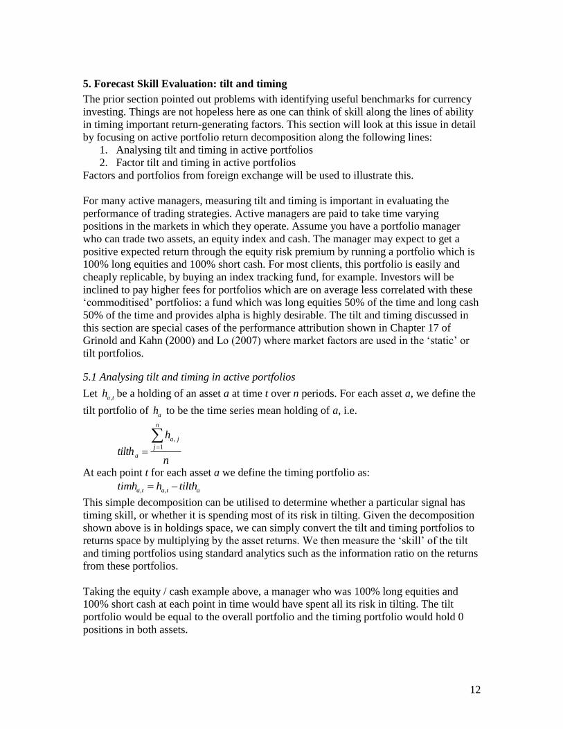
5.1 Analysing tilt and timing in active portfolios

Let ,a th be a holding of an asset a at time t over n periods. For each asset a, we define the

tilt portfolio of ah to be the time series mean holding of a, i.e.

n

h

tilth

n

j

ja

a

1

,

At each point t for each asset a we define the timing portfolio as:

, ,a t a t atimh h tilth

This simple decomposition can be utilised to determine whether a particular signal has

timing skill, or whether it is spending most of its risk in tilting. Given the decomposition

shown above is in holdings space, we can simply convert the tilt and timing portfolios to

returns space by multiplying by the asset returns. We then measure the ‘skill’ of the tilt

and timing portfolios using standard analytics such as the information ratio on the returns

from these portfolios.

Taking the equity / cash example above, a manager who was 100% long equities and

100% short cash at each point in time would have spent all its risk in tilting. The tilt

portfolio would be equal to the overall portfolio and the timing portfolio would hold 0

positions in both assets.

13

Using full sample time series means to determine the tilt exposure of a portfolio is a blunt

tool. A further refinement of this analysis uses a moving window mean to determine the

tilt portfolio. In the analysis below a backward looking window of 3 years of data15

is

used.

We look at simple examples from the foreign exchange market. We use simple decision

rules for succinctness. In fact, this can be thought of as a special case of the mean

variance optimisation process described in Section 2, where in the utility function the

alpha (or return forecast) is equal to the result of the decision rule, the covariance matrix

V is the identity matrix and the transaction cost function TC equals 0.

Example 1

We generate a carry portfolio16

as follows:

1. At the end of every month, rank interest rates in G10 countries

2. For the next month hold a portfolio of +30% currencies with the 3 highest interest

rates, -30% currencies with the 3 lowest interest rates

Example 2

We generate a trend portfolio17

as follows:

1. At the end of each month, rank G10 currencies by spot exchange rate appreciation

(or depreciation) versus US Dollar over the previous 3 months (US Dollar equals

0). We will call this the period over which the foreign exchange appreciation or

depreciation is measured the ‘look back period’.

2. For the next month hold a portfolio of +30% currencies which are highest ranked

in step 1, -30% currencies the 3 currencies which are ranked lowest

Note that the choice of 30% positions in each of these examples is somewhat arbitrary,

although they were used in the Deutsche Bank G10 Currency Future Harvest Index18

. The

15

There is also an issue at the start point with a backward looking moving window. In the analysis below

we have assumed no tilt until there are at least 36 monthly observations. 16

The carry strategy is a very well-known strategy in foreign exchange and has been written about

extensively in both the practitioner and academic world. Burnside, Eichenbaum and Rebelo (2008) look at

the impact of diversification on the carry trade; Burnside, Kleshchelski and Rebelo (2011) look at the

relationship of the carry trade with Peso problems; Menkhoff , Sarno, Schmeling and Schrimpf (2012) look

at the relationship of volatility and liquidity with the carry trade. Lustig, Roussanov and Verdelhan (2011)

show empirical results associating the carry trade with global risk as proxied by global equity market

volatility.

17

Trend following (or momentum) strategies are not solely the province of the foreign exchange world.

The work of Asness, Moskowitz and Pedersen (2009) shows weak momentum effects in most asset classes.

In foreign exchange in particular, Menkhoff and Taylor (2007) give a comprehensive description of trend

following strategies used in the market, and Lequeux and Acar (1998) show that three trend following rules

can help to replicate the trend following style of some investment managers. Burnside, Eichenbaum and

Rebelo (2011) investigate why trend following strategies and carry strategies are successful. Menkhoff ,

Sarno, Schmeling and Schrimpf (forthcoming) show that while momentum does appear to be a meaningful

factor in the foreign exchange markets, it is not easily exploitable.

18

See, for example, https://index.db.com/dbiqweb2/home.do?redirect=search&search=currency+harvest

14

information ratio, the preferred measure of skill in active portfolio management, is

insensitive to the size of the positions chosen here. As mentioned earlier, the information

ratio is a ratio of annualized active return to annualized tracking error, where the active

return is measured as the difference between actual return and a relevant financial

benchmark. In Treynor and Black (1973) this is called the appraisal ratio. This is similar

in spirit to the Sharpe ratio (Sharpe (1994)) where the ratio is annualized excess return to

annualized tracking error, where excess return is measured as the asset return minus the

risk free rate.

The information ratio is not the only analytic which is used to ascribe skill to a trading

strategy. Also important is the consistency of the forecast of returns, so cumulative return

plots are also heavily relied upon in the practitioner community. Statistically, the standard

error bands on these charts are generally very wide, but the ability to forecast returns

consistently is highly valued by clients.

Figure 4 shows the cumulative returns to the tilt, timing and overall strategies. The

performance is calculated from January 1978 to December 2010.

<Figure 4 goes here>

The carry portfolio spends most of its risk in a tilt, whereas the trend portfolio spends

most of its risk in timing. The carry signal is equally effective (performance wise) in tilt

and timing, whereas the trend signal shows only timing skill.

The trend signal construction above uses a 3 month look back period. We vary the look

back period below using 1, 2, 3 and 6 months look back parameters. The table below

shows the information ratio of these different strategies:

'Look back' Information Ratio

1m 0.18

2m 0.29

3m 0.51

6m 0.20

The 3 month look back period dominates in terms of signal performance. In general, an

active manager tries to avoid cherry picking parameters that maximize the backtest

performance: the poor performance using different parameterisations should act as a

warning sign. Indeed, only the 3 month ‘look back’ parameterisation shows statistical

significance. The work of Kahnemann (2011), for example, shows the dangers of

investment managers who believe their own skill over the statistical properties of their

trading strategies. Below we look to see whether there is any more consistent

information we can find from these trend portfolios.

We can combine the trend and carry strategies to build a more complex strategy. Simply

looking at the correlation of the returns from the two different strategies shows they

should be additive:

15

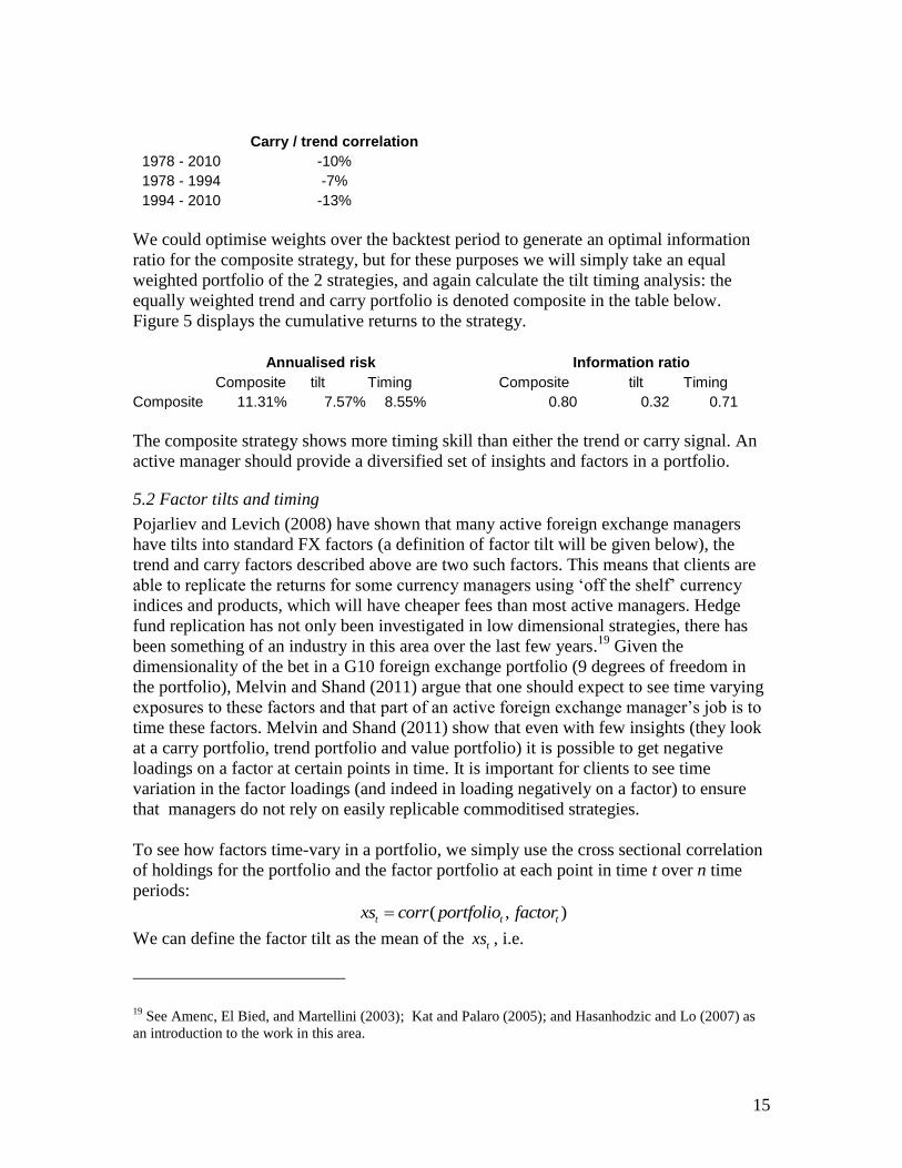
Carry / trend correlation

1978 - 2010 -10%

1978 - 1994 -7%

1994 - 2010 -13%

We could optimise weights over the backtest period to generate an optimal information

ratio for the composite strategy, but for these purposes we will simply take an equal

weighted portfolio of the 2 strategies, and again calculate the tilt timing analysis: the

equally weighted trend and carry portfolio is denoted composite in the table below.

Figure 5 displays the cumulative returns to the strategy.

Annualised risk Information ratio

Composite tilt Timing Composite tilt Timing

Composite 11.31% 7.57% 8.55% 0.80 0.32 0.71

The composite strategy shows more timing skill than either the trend or carry signal. An

active manager should provide a diversified set of insights and factors in a portfolio.

5.2 Factor tilts and timing

Pojarliev and Levich (2008) have shown that many active foreign exchange managers

have tilts into standard FX factors (a definition of factor tilt will be given below), the

trend and carry factors described above are two such factors. This means that clients are

able to replicate the returns for some currency managers using ‘off the shelf’ currency

indices and products, which will have cheaper fees than most active managers. Hedge

fund replication has not only been investigated in low dimensional strategies, there has

been something of an industry in this area over the last few years.19

Given the

dimensionality of the bet in a G10 foreign exchange portfolio (9 degrees of freedom in

the portfolio), Melvin and Shand (2011) argue that one should expect to see time varying

exposures to these factors and that part of an active foreign exchange manager’s job is to

time these factors. Melvin and Shand (2011) show that even with few insights (they look

at a carry portfolio, trend portfolio and value portfolio) it is possible to get negative

loadings on a factor at certain points in time. It is important for clients to see time

variation in the factor loadings (and indeed in loading negatively on a factor) to ensure

that managers do not rely on easily replicable commoditised strategies.

To see how factors time-vary in a portfolio, we simply use the cross sectional correlation

of holdings for the portfolio and the factor portfolio at each point in time t over n time

periods:

( , )t t txs corr portfolio factor

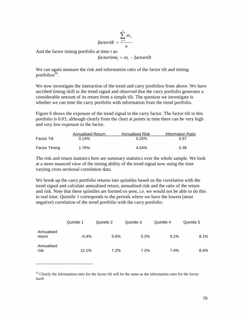
We can define the factor tilt as the mean of the txs , i.e.

19

See Amenc, El Bied, and Martellini (2003); Kat and Palaro (2005); and Hasanhodzic and Lo (2007) as

an introduction to the work in this area.

16

n

xs

factortilt

n

j

j

1

And the factor timing portfolio at time t as:

t tfactortime xs factortilt

We can again measure the risk and information ratio of the factor tilt and timing

portfolios20

.

We now investigate the interaction of the trend and carry portfolios from above. We have

ascribed timing skill to the trend signal and observed that the carry portfolio generates a

considerable amount of its return from a simple tilt. The question we investigate is

whether we can time the carry portfolio with information from the trend portfolio.

Figure 6 shows the exposure of the trend signal to the carry factor. The factor tilt in this

portfolio is 0.03, although clearly from the chart at points in time there can be very high

and very low exposure to the factor. Annualised Return Annualised Risk Information Ratio

Factor Tilt 0.14% 0.25% 0.57 Factor Timing 1.76% 4.54% 0.39

The risk and return statistics here are summary statistics over the whole sample. We look

at a more nuanced view of the timing ability of the trend signal now using the time

varying cross sectional correlation data.

We break up the carry portfolio returns into quintiles based on the correlation with the

trend signal and calculate annualised return, annualised risk and the ratio of the return

and risk. Note that these quintiles are formed ex-post, i.e. we would not be able to do this

in real time. Quintile 1 corresponds to the periods where we have the lowest (most

negative) correlation of the trend portfolio with the carry portfolio.

Quintile 1 Quintile 2 Quintile 3 Quintile 4 Quintile 5

Annualised return -0.4% 5.6% 5.2% 9.1% 8.1%

Annualised risk 12.1% 7.2% 7.2% 7.4% 8.4%

20

Clearly the information ratio for the factor tilt will be the same as the information ratio for the factor

itself.

17

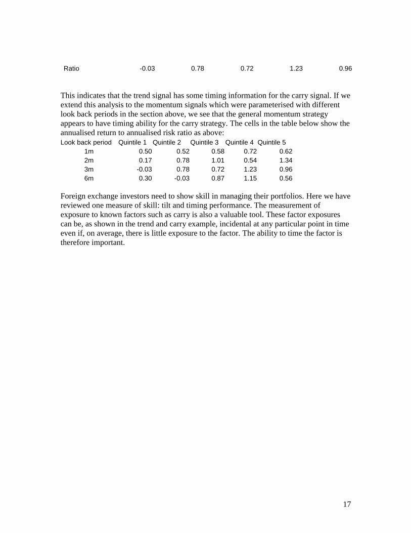
Ratio -0.03 0.78 0.72 1.23 0.96

This indicates that the trend signal has some timing information for the carry signal. If we

extend this analysis to the momentum signals which were parameterised with different

look back periods in the section above, we see that the general momentum strategy

appears to have timing ability for the carry strategy. The cells in the table below show the

annualised return to annualised risk ratio as above:

Look back period Quintile 1 Quintile 2 Quintile 3 Quintile 4 Quintile 5

1m 0.50 0.52 0.58 0.72 0.62

2m 0.17 0.78 1.01 0.54 1.34

3m -0.03 0.78 0.72 1.23 0.96

6m 0.30 -0.03 0.87 1.15 0.56

Foreign exchange investors need to show skill in managing their portfolios. Here we have

reviewed one measure of skill: tilt and timing performance. The measurement of

exposure to known factors such as carry is also a valuable tool. These factor exposures

can be, as shown in the trend and carry example, incidental at any particular point in time

even if, on average, there is little exposure to the factor. The ability to time the factor is

therefore important.

18

6. Enhancing Forecasts with Conditioners

Currency investors employ forecasts with the aim of generating attractive risk-adjusted

returns. In the prior section we saw that a static tilt into the carry trade can generate long-

run profitable strategies. In fact, if one believed the Meese-Rogoff result of a random

walk being the best forecast of future spot returns in currencies, this might imply that the

carry trade is a reasonable investment strategy as you never should expect the exchange

rate to change from the current spot rate. But empirical analysis teaches that the ability to

profit from interest differentials without offsetting exchange rate movements is

threatened by exchange rate volatility. So even if one accepts that a random walk is the

best forecast at a point in time looking forward, ex-post, we know that exchange rates

will change from the current spot rate so that the greater the expected volatility, the

greater the threat to a successful carry strategy. We should expect carry trades to deliver

positive returns in normal market conditions but underperform in periods of financial

market stress, when volatility spikes. The best investors have skill in timing factors,

dialing risk up when a strategy outperforms and turning risk down when drawdown

periods are realized, so in the case of carry trades, a measure of market stress can be a

useful input into investing. Melvin and Taylor (2009) developed such a stress index and

showed that it offered potential for enhancing returns to the carry trade. Such a general

financial stress index (FSI) is similar in some respects to the index recently proposed by

the International Monetary Fund (IMF) (IMF, 2008).21

However, an important difference

between the FSI and the IMF version is that in operationalizing the FSI we do not use

full-sample data in constructing the index (e.g. by fitting generalised autoregressive

conditional heteroskedasticity, GARCH, models using the full-sample data or subtracting

off full-sample means). This is important as investors do not have the advantage of

perfect foresight in calibrating models and must, therefore, analyze models using only

what is known in real time in each period. The FSI is built for the same group of

seventeen developed countries as in the IMF study, namely: Australia, Austria, Belgium,

Canada, Denmark, Finland, France, Germany, Italy, Japan, Netherlands, Norway, Spain,

Sweden, Switzerland, the UK and the USA. In contrast to the IMF analysis, however, we

built a ‘global’ FSI based on an average of the individual FSI for each of these seventeen

countries.

The FSI is a composite variable built using market-based indicators in order to capture

four essential characteristics of a financial crisis: large shifts in asset prices, an abrupt

increase in risk and uncertainty, abrupt shifts in liquidity and a measurable decline in

banking system health indicators.

In the banking sector, three indicators were used:

i) The beta of banking sector stocks, constructed as the twelve-month rolling

covariance of the year-over-year percent change of a country’s banking sector

equity index and its overall stock market index, divided by the rolling twelve-

month variance of the year-over-year percent change of the overall stock

market index.

21

See also Illing and Liu (2006).

19

ii) The spread between interbank rates and the yield on Treasury Bills, i.e. the so-

called TED spread that we discussed above: three-month LIBOR or

commercial paper rate minus the government short-term rate.

iii) The slope of the yield curve, or inverted term spread: the government short-

term Treasury Bill yield minus the government long-term bond yield.

In the securities market, a further three indicators were used:

i) Corporate bond spreads: the corporate bond yield minus the long-term

government bond yield.

ii) Stock market returns: the monthly percentage change in the country equity

market index.

iii) Time-varying stock return volatility. This was calculated as the square root of

an exponential moving average of squared deviations from an exponential

moving average of national equity market returns. An exponential moving

average with a 36-month half-life was used in both cases.

Finally, in the foreign exchange market:

iv) For each country a time-varying measure of real exchange rate volatility was

similarly calculated – i.e. the square root of an exponential moving average of

squared deviations from an exponential moving average of monthly

percentage real effective exchange rate changes. An exponential moving

average with a 36-month half-life was used in both cases.

All components of the FSI are in monthly frequency and each component is scaled to be

equal to 100 at the beginning of the sample. A national FSI index is constructed for each

country by taking an equally weighted average of the various components. Then, a global

FSI index is constructed by taking an equally weighted average of the seventeen national

FSI indices. The calculated global FSI series runs from December 1983 until October

2008.22

In order to ascertain whether an extreme value of the FSI has been breached, we scored

the FSI by subtracting off a time-varying mean (calculated using an exponential moving

average with a 36-month half-life) and dividing through by a time-varying standard

deviation (calculated taking the square root of an exponential moving average, with a 36-

month half-life, of the squared deviations from the time-varying mean). The resulting

scored FSI gives a measure of how many standard deviations the FSI is away from its

time-varying mean.

As can be seen from Figure 7, the global FSI crosses the threshold of one standard

deviation above the mean for most of the major crises of the past twenty years or so,

including the 1987 stock market crash, the Nikkei/junk bond collapse of the late 1980s,

the 1990 Scandinavian banking crisis and the 1998 Russian default/LTCM crisis. The

1992 ERM crisis is less evident at the global level.

22

No doubt, one can fine-tune the FSI in terms of weighting components and countries as a function of

contribution to performance. Here we follow the IMF approach, but for any particular application, one

could probably extend the analysis and achieve some marginal improvement in results.

20

Most interestingly, however, the global FSI shows a very marked effect during the recent

crisis. Mirroring the carry unwind in August 2007 that we documented above, there is a

brief lull in the FSI as it drops below one standard deviation from its mean before leaping

up again in November 2007 to nearly 1.5 standard deviations from the mean. The global

FSI then breaches the two-standard deviation threshold in January 2008 and again in

March 2008 (coinciding with the near collapse of Bear Stearns). With the single

exception of a brief lull in May 2008, when the global FSI falls to about 0.7 standard

deviations above the mean, it then remains more than one standard deviation above the

mean for the rest of the sample, spiking up in October to more than four standard

deviations from the mean following the Lehman Brothers debacle in September.23

It is tempting to infer from this analysis that an active currency manager could have

significantly defended their portfolio by taking risk off (or perhaps even going short

carry) in August 2007, especially as the carry unwind that occurred that month is

confirmed as a crisis point by the movements in the global FSI in the same month. We

carried out a first exploration of this idea by estimating a Probit model of significant

drawdowns from the carry trade investment as a function of the global FSI, where a

“significant drawdown” is defined as greater than a one standard deviation negative

return. Table 4 presents the specification and estimation results. Clearly, the probability

of a major drawdown from a carry trade investment is increasing in the FSI. Table 4

yields evidence of statistical significance of the effect of the FSI on the carry trade.24

What about economic significance?

To examine the economic significance of the FSI effects on carry trade returns, we

simulate the returns an investor would earn from investing in the Deutsche Bank Carry

Return Index (long the 3 highest yielding currencies and short the 3 lowest yielding

currencies across the developed markets). Suppose the investor just invests in the index in

an unconditional sense, without regard to market conditions. We will call this the

“Unconditional Return.” Alternatively, the investor can invest in the index in “normal”

periods and close out the position in stressful periods, where stress is measured by the

global FSI. Specifically, when the FSI exceeds a value of 1, the carry trade exposure is

shut off; otherwise, the investment is held. Figure 8 illustrates the cumulative returns to

such strategies. The cumulative unconditional return is -1% while the conditional return

is +38% over the period studied.25

23

Apart from financial forecasting, a measure like the FSI could be useful for policymakers to gauge the

stresses in financial markets to help inform monetary and fiscal decisions. 24

A consideration of factors that might control carry trade losses is receiving increased attention in the

literature lately. Some examples are Brunnermeier, Nagel, and Pedersen (2008); Jurek (2007); Clarida,

Davis, and Pedersen (2009); Habib and Straccca (2012); and Jorda and Taylor (forthcoming). 25

Recall that the FSI only uses information known at each point in time in the sample, there is no peek-

ahead in the data. In addition, these results are achieved with the arbitrary choice of FSI threshold of one

standard deviation with no specification search over alternative cut-offs,

21

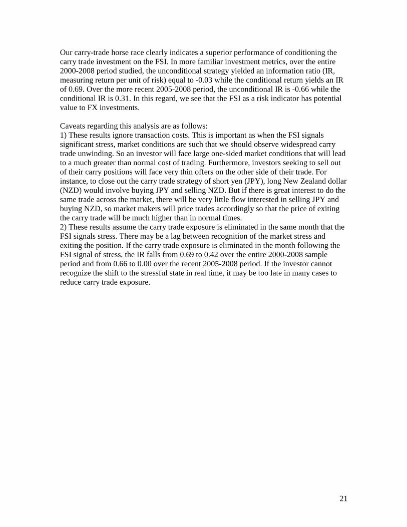
Our carry-trade horse race clearly indicates a superior performance of conditioning the

carry trade investment on the FSI. In more familiar investment metrics, over the entire

2000-2008 period studied, the unconditional strategy yielded an information ratio (IR,

measuring return per unit of risk) equal to -0.03 while the conditional return yields an IR

of 0.69. Over the more recent 2005-2008 period, the unconditional IR is -0.66 while the

conditional IR is 0.31. In this regard, we see that the FSI as a risk indicator has potential

value to FX investments.

Caveats regarding this analysis are as follows:

1) These results ignore transaction costs. This is important as when the FSI signals

significant stress, market conditions are such that we should observe widespread carry

trade unwinding. So an investor will face large one-sided market conditions that will lead

to a much greater than normal cost of trading. Furthermore, investors seeking to sell out

of their carry positions will face very thin offers on the other side of their trade. For

instance, to close out the carry trade strategy of short yen (JPY), long New Zealand dollar

(NZD) would involve buying JPY and selling NZD. But if there is great interest to do the

same trade across the market, there will be very little flow interested in selling JPY and

buying NZD, so market makers will price trades accordingly so that the price of exiting

the carry trade will be much higher than in normal times.

2) These results assume the carry trade exposure is eliminated in the same month that the

FSI signals stress. There may be a lag between recognition of the market stress and

exiting the position. If the carry trade exposure is eliminated in the month following the

FSI signal of stress, the IR falls from 0.69 to 0.42 over the entire 2000-2008 sample

period and from 0.66 to 0.00 over the recent 2005-2008 period. If the investor cannot

recognize the shift to the stressful state in real time, it may be too late in many cases to

reduce carry trade exposure.

22

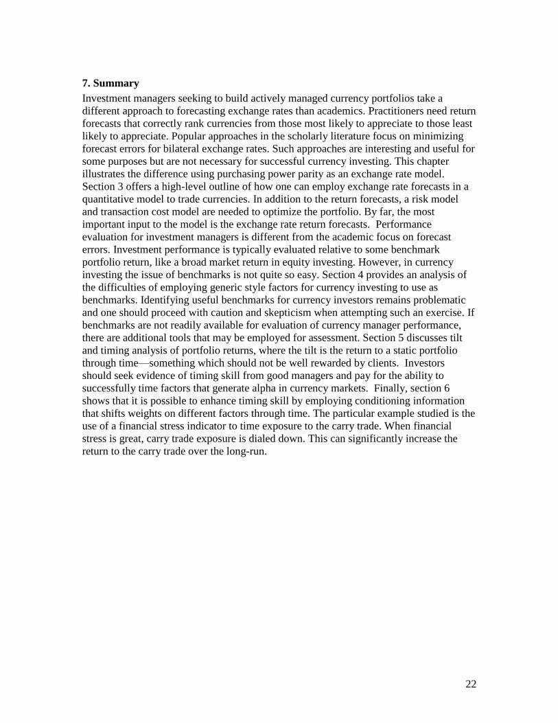
7. Summary

Investment managers seeking to build actively managed currency portfolios take a

different approach to forecasting exchange rates than academics. Practitioners need return

forecasts that correctly rank currencies from those most likely to appreciate to those least

likely to appreciate. Popular approaches in the scholarly literature focus on minimizing

forecast errors for bilateral exchange rates. Such approaches are interesting and useful for

some purposes but are not necessary for successful currency investing. This chapter

illustrates the difference using purchasing power parity as an exchange rate model.

Section 3 offers a high-level outline of how one can employ exchange rate forecasts in a

quantitative model to trade currencies. In addition to the return forecasts, a risk model

and transaction cost model are needed to optimize the portfolio. By far, the most

important input to the model is the exchange rate return forecasts. Performance

evaluation for investment managers is different from the academic focus on forecast

errors. Investment performance is typically evaluated relative to some benchmark

portfolio return, like a broad market return in equity investing. However, in currency

investing the issue of benchmarks is not quite so easy. Section 4 provides an analysis of

the difficulties of employing generic style factors for currency investing to use as

benchmarks. Identifying useful benchmarks for currency investors remains problematic

and one should proceed with caution and skepticism when attempting such an exercise. If

benchmarks are not readily available for evaluation of currency manager performance,

there are additional tools that may be employed for assessment. Section 5 discusses tilt

and timing analysis of portfolio returns, where the tilt is the return to a static portfolio

through time—something which should not be well rewarded by clients. Investors

should seek evidence of timing skill from good managers and pay for the ability to

successfully time factors that generate alpha in currency markets. Finally, section 6

shows that it is possible to enhance timing skill by employing conditioning information

that shifts weights on different factors through time. The particular example studied is the

use of a financial stress indicator to time exposure to the carry trade. When financial

stress is great, carry trade exposure is dialed down. This can significantly increase the

return to the carry trade over the long-run.

23

References

Amenc, N., El Bied, S., and Martellini, L., 2003. Predictability in hedge fund returns,

Financial Analysts Journal. 59, 32-46.

Bessembinder, H., 1994. Bid-ask spreads in the interbank foreign exchange markets.

Journal of Financial Economics. 35, 317-348.

Bollerslev, T., Engle, R.F., Wooldridge, J.M., 1988. A capital asset pricing model with

time-varying covariances. Journal of Political Economy. 96, 116-131.

Bollerslev, T., Melvin, M., 1994. Bid-ask spreads and volatility in the foreign exchange

market. Journal of International Economics. 36, 355-372.

Brunnermeir , M., Nagel, S., Pedersen, L., 2008. Carry trades and currency crashes.

NBER Macroeconomics Annual, 2008.

Burnside, C., Eichenbaum, M., and Rebelo, S., 2008. Carry trade: the gains from

diversification. Journal of the European Economic Association. 6(2-3), 581-588.

Burnside, C., Eichenbaum, M., and Rebelo, S., 2011. Carry trade and momentum in

currency markets. Annual Review of Financial Economics. 3, 511-535.

Burnside, C., Kleshchelski, I., and Rebelo, S., 2011. Do peso problems explain the

returns to the carry trade. Review of Financial Studies . 24, 853-891.

Cheung, Y., Chinn, M, and Pascual, A. G., 2005. Empirical exchange rate models of the

nineties: are any fit to survive? Journal of International Money and Finance. 24, 1150-

1175.

Christensen, K., Kinnebrock, S., and Podolskij, M., 2010. Pre-averaging estimators of the

ex-post covariance matrix in noisy diffusion models with non-synchronous data. Journal

of Econometrics. 159, 116-133.

Clarida, R., Davis, J., Pedersen, N., 2009. Currency carry trade regimes: Beyond the

Fama regression. Journal of International Money and Finance. 28, 1375-1389.

Della Corte, Pasquale, Sarno, Lucio, and Tsiakas, Ilias, 2009. An economic evaluation of

empirical exchange rate models. The Review of Financial Studies. 22, 3491-3530.

De Zwart, G., Markwat, T., Swinkels, L. and van Dijk, D. 2009. The economic value of

fundamental and technical information in emerging currency markets. Journal of

International Money and Finance. 28, 581-604.

24

Elliott, G. and Ito, T., 1999. Heterogeeneous expectations and test of efficiency in the

yen/dollar forward exchange rate market. Journal of Monetary Economics. 43, 435-456.

Engel, C., Mark, N.C., and West, K.D., 2007. Exchange rate models are not as bad as you

think. NBER Macroeconomics Annual. 381-441.

Evans, M.D.D., 2011. Exchange Rate Dynamics. Princeton Univ Press, Princeton.

Frankel, J.A. and Rose, A.K., 1995. Empirical research on nominal exchange rates.

Handbook of International Economics. 3, Elsevier, Amsterdam.

Glassman, D. 1987. Exchange rate risk and transactions costs: Evidence from bid-ask

spreads. Journal of International Money and Finance. 6, 479-490.

Grinold, R and Kahn, R., 2000. Active Portfolio Management. McGraw Hill, New York.

Habib, M.M. and Stracca, L., 2012. Getting beyond carry trade: What makes a safe haven

currency? Journal of International Economics. 87, 50-64.

Hartmann, P. 1999. Trading volumes and transaction costs in the foreign exchange

market: Evidence from daily dollar-yen spot data. Journal of Banking and Finance. 23,

891-824.

Hasanhodzic, J. and Lo, A., 2007. Can hedge fund returns be replicated?: The linear case.

Journal oF Investment Management. 5, 5–45.

Illing, M. and Liu, Y., 2006. Measuring financial stress in a developed country: an

application to Canada. Journal of Financial Stability. 2, 243-265.

James, J., 2003. Simple trend-following strategies in currency trading. Quantitative

Finance. 3, C75-C77.

Jorda, O. and Taylor, A.M., forthcoming. The carry trade and fundamentals: Nothing to

fear but FEER itself. Journal of International Economics.

Jorion, P., 1985. International portfolio diversification with estimation risk. The Journal

of Business. 58, 259-278.

Jurek, J., 2007. Crash-neutral currency carry trades. Princeton, Bendheim Center for

Finance. Working Paper.

Kahneman, D., 2011. Thinking fast and slow. Allen Lane, London.

Kat, H. and Palaro, H., 2005. Hedge fund returns: you can make them yourself!

Journal of Wealth Management. 8, 62-68.

25

Konno, H. and Yamazaki, H., 1991. Mean-absolute deviation portfolio optimization

model and its applications to Tokyo stock market. Management Science. 37, 519-531.

Kroner, K.E. and Ng, V.K., 1998. Modeling asymmetric comovements of asset returns.

Review of Financial Studies. 11, 817-844.

Ledoit, O. and Wolf, M., 2004. Honey, I shrunk the sample covariance matrix. The

Journal of Portfolio Management. 30, 110-119.

Lequeux, P. and Acar. E., 1998. A dynamic index for managed currencies funds using

CME currency contracts. European Journal of Finance. 4, 311-330.

Lo, A., 2002. The Statistics of Sharpe Ratios. Financial Analysts Journal. 58, 36-52.

Lo, A., 2007. Where do alphas come from?: A new measure of the value of active

investment management. Journal of Investment Management. 6, 1–29.

Lustig, H., Roussanov, N and Verdelhan A., 2011. Common risk factors in currency

Markets. Review of Financial Studies. 24, 3731-3777.

Meese, R. and Rogoff, K., 1983. Empirical exchange rate models of the seventies: Do

they fit out of sample? Journal of International Economics. 14, 3-24.

Melvin, M. and Shand, D., 2011. Active currency investing and performance

benchmarks. The Journal of Portfolio Management. 37, 46-59.

Melvin, M. and Taylor, M., 2009. The crisis in the foreign exchange market. Journal of

International Money and Finance. 28, 1317-1330.

Menkhoff, L. and Taylor, M., 2007. The obstinate passion of foreign exchange

professionals: Technical Analysis. Journal of Economic Literature. 45, 935-972.

Menkhoff, L., Schmeling, M., Sarno, L., and Schrimpf, A., 2012. Carry trades and global

foreign exchange volatility. Journal of Finance. 67, 681-718.

Menkhoff, L., Schmeling, M., Sarno, L., and Schrimpf, A., Forthcoming. Currency

momentum strategies. Journal of Financial Economics.

Naranjo, A., and Nimalendran, M., 2000. Government intervention and adverse selection

costs in foreign exchange markets. The Review of Financial Studies. 13, 453-477.

Neely, C., Weller, P. and Ulrich, J. 2009. The adaptive markets hypothesis: Evidence

from the foreign exchange market. Journal of Financial and Quantitative Analysis. 44,

467-488.

26

Obstfeld, M, and Rogoff, K., 2001. The six major puzzles in international

macroeconomics: is there a common cause? In Rogoff, K. and Bernanke, B., eds. ,NBER

Macroeconomics Annual 2000. 15, MIT Press, p. 339-412.

Okunev, J. and White, D. 2003. Do momentum-based strategies still work in foreign

currency markets? Journal of Financial and Quantitative Analysis. 425-447.

Paape, C. 2003. Currency overlay in performance evaluation. Financial Analysts Journal.

59, 55-68.

Pojarliev, M., Levich, R., 2008. Do professional currency managers beat the benchmark?

Financial Analysts Journal. 64, 18-32.

Pojarliev, M. and Levich, R. 2010. Trades of the living dead: Style differences, style

persistence and performance of currency fund managers. Journal of International Money

and Finance. 29, 1752-1775.

Pojarliev, M. and Levich, R. 2011. Are all currency managers equal? Journal of Portfolio

Management. 37, 42-53.

Ramadorai, T., 2008. What determines transaction costs in foreign exchange markets?

International Journal of Finance and Economics. 13, 14-25.

Sarno, L. and Taylor, M.P., 2002. The economics of exchange rates. Cambridge Univ

Press, Cambridge.

Satchell, S. and Timmermann, A., 1995. An assessment of the economic value of non-

linear foreign exchange rate forecasts. Journal of Forecasting. 14, 477-497.

Shanken, J., 1987. Nonsynchronous data and the covariance-factor structure of returns.

Journal of Finance. 42, 221-231.

Sharpe, W. F., 1994. The Sharpe ratio. Journal of Portfolio Management. 21. 49-59.

Stevens, G., 1998. On the inverse of the covariance matrix in portfolio analysis, Journal

of Finance. 53, 1821-1827.

Taylor, M.P., 1995. The economics of exchange rates. Journal of Economic Literature. 33,

13-47.

Treynor, J. and Black, F., 1973. How to use security analysis to improve portfolio

selection. Journal of Business. 46, 66-86.

Williamson, J. 2009. Exchange rate economics. Open Economies Review. 20, 123-14

27

Figures

Figure 1

Spot rates and fair value according to purchasing power parity

Spot and Purchasing Power Parity, 1980-2010

80 82 85 87 90 92 95 97 00 02 05 07 10

100

150

200

250

JP

spot

ppp

80 82 85 87 90 92 95 97 00 02 05 07 10

0.5

0.6

0.7

0.8

0.9

GB

80 82 85 87 90 92 95 97 00 02 05 07 10

1

1.5

2

2.5

CH

80 82 85 87 90 92 95 97 00 02 05 07 10

1

1.5

2

AU

80 82 85 87 90 92 95 97 00 02 05 07 10

1

1.2

1.4

1.6

CA

80 82 85 87 90 92 95 97 00 02 05 07 10

1

1.5

2

2.5

NZ

80 82 85 87 90 92 95 97 00 02 05 07 10

6

8

10

SE

80 82 85 87 90 92 95 97 00 02 05 07 10

5

6

7

8

9

NO

28

Figure 2

Performance of portfolio of currencies ranked by deviation from PPP

This portfolio is rebalanced monthly at the beginning of each month, beginning in 1981:1

and ending in 2010:12. It is a sum-to-zero, long-short portfolio with positions in the US

dollar, Japanese yen, British pound, Swiss franc, Canadian dollar, Australian dollar, New

Zealand dollar, Swedish krona and Norwegian kroner. The information ratio of the

portfolio’s performance over the full sample is 0.5.

80 82 84 86 88 90 92 94 96 98 00 02 04 06 08 10 120

0.02

0.04

0.06

0.08

0.1

0.12

0.14

0.16

0.18

Cumulative performance of PPP portfolio

29

Figure 3

Cumulative Returns to Trend Following Strategies

The figure displays the cumulative returns to momentum or trend investment strategies offered by indexes created by AFX, Credit

Suisse, and Deutsche Bank.

88 90 92 94 96 98 00 02 04 06 08 10-20

-10

0

10

20

30

40

50

60

70

80

Cumulative Returns to Trend Following Strategies

AFX

CS

DB

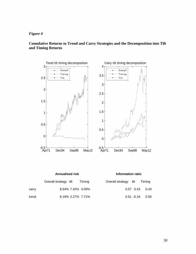
30

Figure 4

Cumulative Returns to Trend and Carry Strategies and the Decomposition into Tilt

and Timing Returns

Annualised risk Information ratio

Overall strategy tilt Timing Overall strategy tilt Timing

carry 8.64% 7.42% 4.09% 0.57 0.43 0.43

trend 8.19% 2.27% 7.71% 0.51 -0.16 0.56

Apr71 Dec84 Sep98 May12-0.5

0

0.5

1

1.5

2

2.5

3Trend tilt timing decomposition

Overa l l

T im ing

Ti lt

Apr71 Dec84 Sep98 May12-0.5

0

0.5

1

1.5

2

2.5

3

3.5

4Carry tilt timing decomposition

Overa l l

T im ing

Ti lt

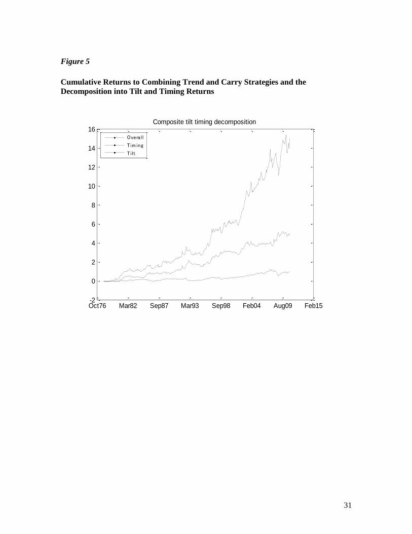
31

Figure 5

Cumulative Returns to Combining Trend and Carry Strategies and the

Decomposition into Tilt and Timing Returns

Oct76 Mar82 Sep87 Mar93 Sep98 Feb04 Aug09 Feb15-2

0

2

4

6

8

10

12

14

16Composite tilt timing decomposition

Overa l l

T im ing

Ti lt

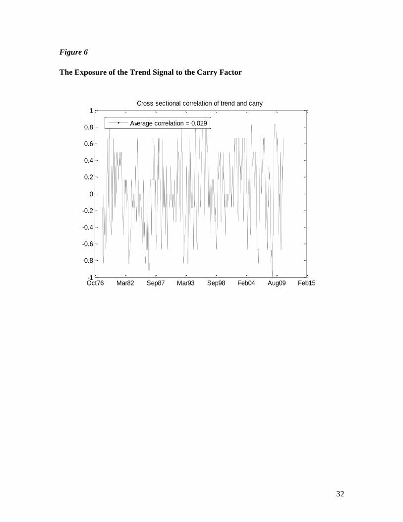
32

Figure 6

The Exposure of the Trend Signal to the Carry Factor

Oct76 Mar82 Sep87 Mar93 Sep98 Feb04 Aug09 Feb15-1

-0.8

-0.6

-0.4

-0.2

0

0.2

0.4

0.6

0.8

1Cross sectional correlation of trend and carry

Average correlation = 0.029

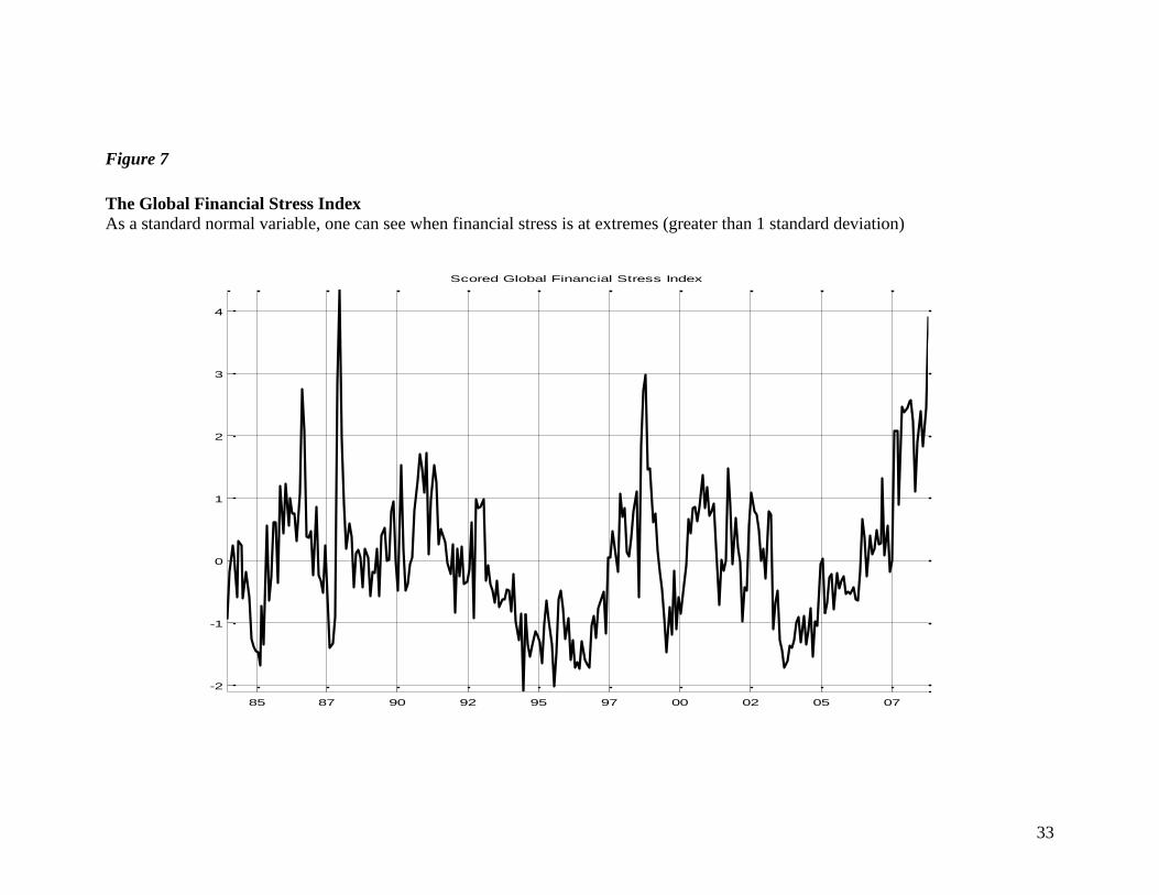
33

Figure 7

The Global Financial Stress Index

As a standard normal variable, one can see when financial stress is at extremes (greater than 1 standard deviation)

85 87 90 92 95 97 00 02 05 07

-2

-1

0

1

2

3

4

Scored Global Financial Stress Index

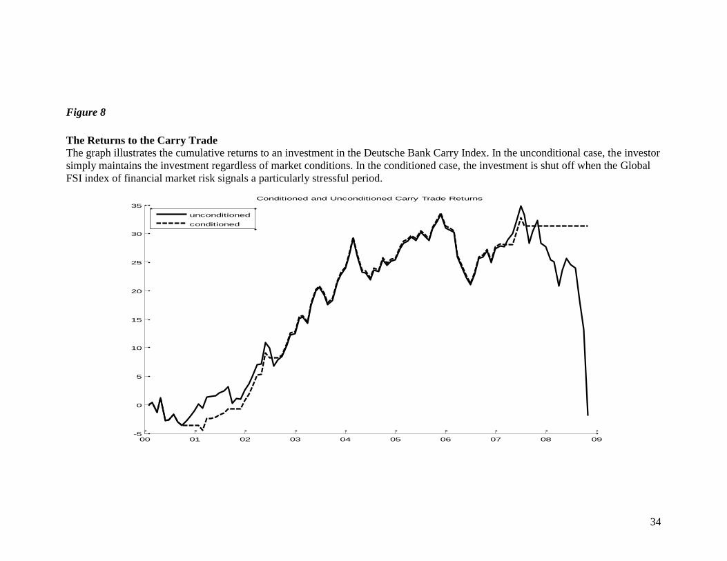
34

Figure 8

The Returns to the Carry Trade

The graph illustrates the cumulative returns to an investment in the Deutsche Bank Carry Index. In the unconditional case, the investor

simply maintains the investment regardless of market conditions. In the conditioned case, the investment is shut off when the Global

FSI index of financial market risk signals a particularly stressful period.

00 01 02 03 04 05 06 07 08 09-5

0

5

10

15

20

25

30

35

Conditioned and Unconditioned Carry Trade Returns

unconditioned

conditioned

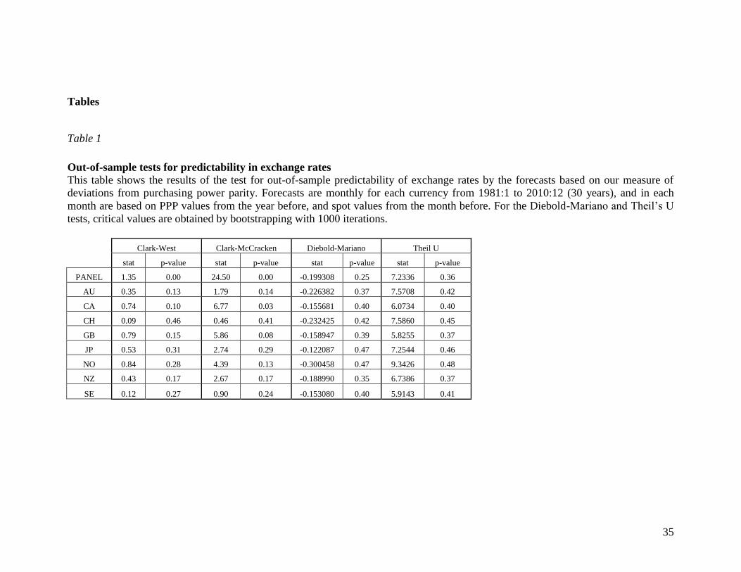
35

Tables

Table 1

Out-of-sample tests for predictability in exchange rates

This table shows the results of the test for out-of-sample predictability of exchange rates by the forecasts based on our measure of

deviations from purchasing power parity. Forecasts are monthly for each currency from 1981:1 to 2010:12 (30 years), and in each

month are based on PPP values from the year before, and spot values from the month before. For the Diebold-Mariano and Theil’s U

tests, critical values are obtained by bootstrapping with 1000 iterations.

Clark-West Clark-McCracken Diebold-Mariano Theil U

stat p-value stat p-value stat p-value stat p-value

PANEL 1.35 0.00 24.50 0.00 -0.199308 0.25 7.2336 0.36

AU 0.35 0.13 1.79 0.14 -0.226382 0.37 7.5708 0.42

CA 0.74 0.10 6.77 0.03 -0.155681 0.40 6.0734 0.40

CH 0.09 0.46 0.46 0.41 -0.232425 0.42 7.5860 0.45

GB 0.79 0.15 5.86 0.08 -0.158947 0.39 5.8255 0.37

JP 0.53 0.31 2.74 0.29 -0.122087 0.47 7.2544 0.46

NO 0.84 0.28 4.39 0.13 -0.300458 0.47 9.3426 0.48

NZ 0.43 0.17 2.67 0.17 -0.188990 0.35 6.7386 0.37

SE 0.12 0.27 0.90 0.24 -0.153080 0.40 5.9143 0.41

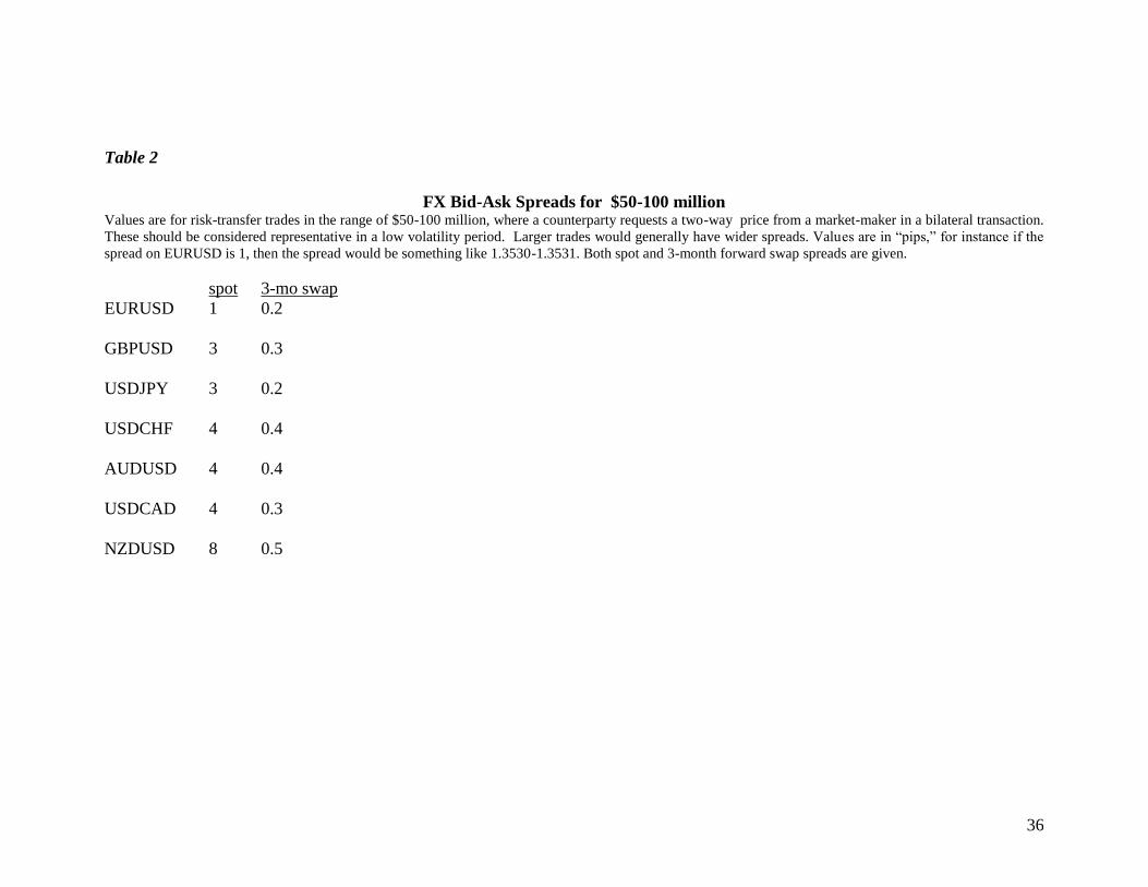
36

Table 2

FX Bid-Ask Spreads for $50-100 million Values are for risk-transfer trades in the range of $50-100 million, where a counterparty requests a two-way price from a market-maker in a bilateral transaction.

These should be considered representative in a low volatility period. Larger trades would generally have wider spreads. Values are in “pips,” for instance if the

spread on EURUSD is 1, then the spread would be something like 1.3530-1.3531. Both spot and 3-month forward swap spreads are given.

spot 3-mo swap

EURUSD 1 0.2

GBPUSD 3 0.3

USDJPY 3 0.2

USDCHF 4 0.4

AUDUSD 4 0.4

USDCAD 4 0.3

NZDUSD 8 0.5

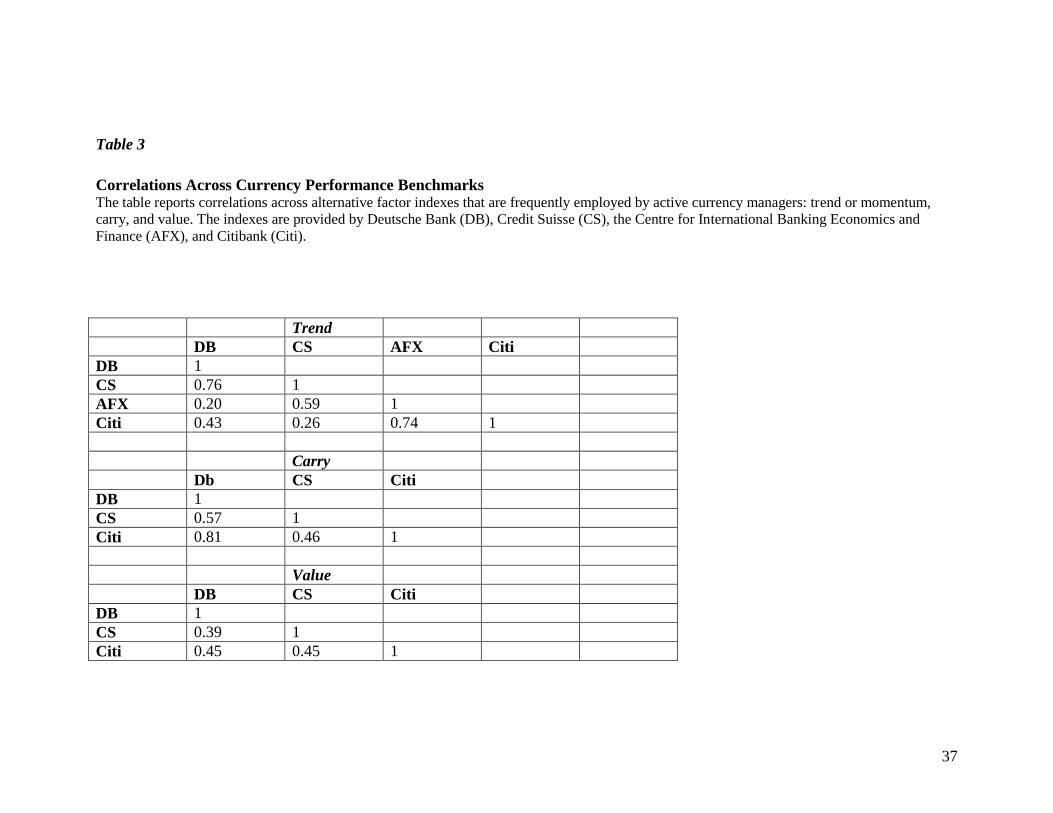
37

Table 3

Correlations Across Currency Performance Benchmarks The table reports correlations across alternative factor indexes that are frequently employed by active currency managers: trend or momentum,

carry, and value. The indexes are provided by Deutsche Bank (DB), Credit Suisse (CS), the Centre for International Banking Economics and

Finance (AFX), and Citibank (Citi).

Trend

DB CS AFX Citi

DB 1

CS 0.76 1

AFX 0.20 0.59 1

Citi 0.43 0.26 0.74 1

Carry

Db CS Citi

DB 1

CS 0.57 1

Citi 0.81 0.46 1

Value

DB CS Citi

DB 1

CS 0.39 1

Citi 0.45 0.45 1

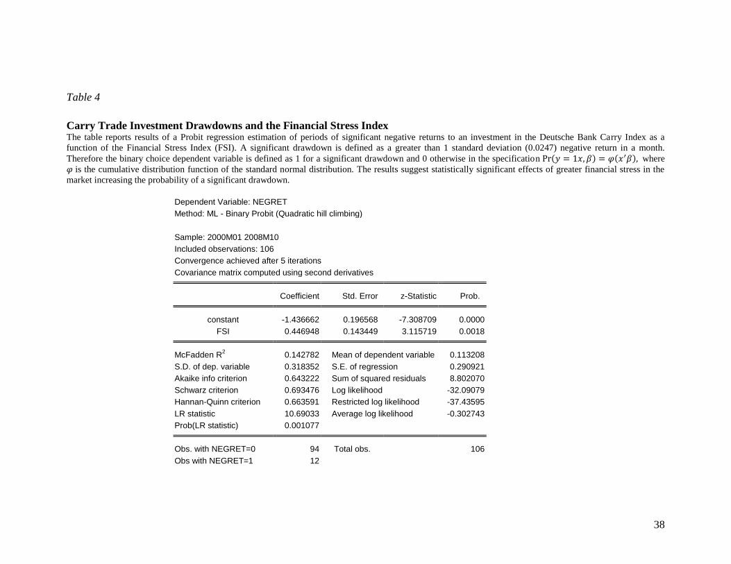
38

Table 4

Carry Trade Investment Drawdowns and the Financial Stress Index The table reports results of a Probit regression estimation of periods of significant negative returns to an investment in the Deutsche Bank Carry Index as a

function of the Financial Stress Index (FSI). A significant drawdown is defined as a greater than 1 standard deviation (0.0247) negative return in a month.

Therefore the binary choice dependent variable is defined as 1 for a significant drawdown and 0 otherwise in the specification ( ) ( ) where

is the cumulative distribution function of the standard normal distribution. The results suggest statistically significant effects of greater financial stress in the

market increasing the probability of a significant drawdown.

Dependent Variable: NEGRET

Method: ML - Binary Probit (Quadratic hill climbing)

Sample: 2000M01 2008M10

Included observations: 106

Convergence achieved after 5 iterations

Covariance matrix computed using second derivatives Coefficient Std. Error z-Statistic Prob.

constant -1.436662 0.196568 -7.308709 0.0000

FSI 0.446948 0.143449 3.115719 0.0018

McFadden R2 0.142782 Mean of dependent variable 0.113208

S.D. of dep. variable 0.318352 S.E. of regression 0.290921

Akaike info criterion 0.643222 Sum of squared residuals 8.802070

Schwarz criterion 0.693476 Log likelihood -32.09079

Hannan-Quinn criterion 0.663591 Restricted log likelihood -37.43595

LR statistic 10.69033 Average log likelihood -0.302743

Prob(LR statistic) 0.001077

Obs. with NEGRET=0 94 Total obs. 106

Obs with NEGRET=1 12