forecasting dr. everette s. gardner, jr.. forecasting 2 judgment exercises exercise 1 finished files...
TRANSCRIPT

ForecastingForecasting
Dr. Everette S. Gardner, Jr.

Forecasting 2
Judgment exercises
Exercise 1
Finished files are the result of years of scientific study combined with the experience of years.
How many times does the letter F appear in the sentence above? Count them only once; do not go back and count them again. ________
How confident are you in your answer? Rate your confidence on a scale of 0 to 100, where 0 means that you are sure you are wrong, and 100 means that you are sure you right. _________

Forecasting 3
Judgment exercises (cont.)
Exercise 2
Threatened by a superior enemy force, the general faces a dilemma. His intelligence officers say his soldiers will be caught in an ambush in which 600 of them will die unless he leads them to safety by one of two available routes. If he takes the first route, 200 soldiers will be saved. If he takes the second route, there’s a one-third chance that 600 soldiers will be saved and a two-thirds chance that none will be saved. Which route should he take? ________

Forecasting 4
Judgment exercises (cont.)
Exercise 3
The general again has to choose between two escape routes. But this time his aides tell him that if he takes the first, 400 soldiers will die. If he takes the second, there’s a one-third chance that no soldiers will die, and a two-thirds chance that 600 soldiers will die. Which route should he take? _______

Forecasting 5
Judgment exercises (cont.)
Exercise 4
Linda is 31, single, outspoken, and very bright. She majored in philosophy in college. As a student, she was deeply concerned with discrimination and other social issues, and participated in anti-nuclear demonstrations. Which statement is more likely?a. Linda is a bank teller.b. Linda is a bank teller and active in the feminist
movement._______

Forecasting 6
Human biases in forecasting
Company Politics● Forecast what the boss wants to hear
Overconfidence● Confidence has no relation to accuracy
Wishful thinking● Optimistic forecasts more probable
Success/failure attribution● Good forecasts due to skill, bad due to chance

Forecasting 7
Human biases in forecasting
Gambler’s fallacy● Bad luck and good luck will balance out
Data presentation● Misleading graphs/tables easily accepted
Conservatism● Refusal to accept drastic change

Forecasting 8
Forecasting methods
Human judgment● Subject to bias and inconsistency● Models usually beat humans
Time series forecasting● Based on analysis of past history● Cheap and easy● On average, most accurate method● Should always be attempted

Forecasting 9
Forecasting methods (cont.)
Regression modeling● Based on causal relationships● Expensive and difficult● Must forecast independent variables
Growth or market development models● Based on assumed growth patterns● Cheap and easy● Difficult to validate
Forecasting 10
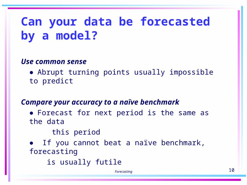
Can your data be forecastedby a model?
Use common sense● Abrupt turning points usually impossible to predict
Compare your accuracy to a naïve benchmark● Forecast for next period is the same as the data
this period● If you cannot beat a naïve benchmark, forecasting is usually futile

Forecasting 11
Forecast profiles
Additive Multiplicative Nonseasonal Seasonality Seasonality
Constant
Level
Linear Trend
Exponential
Trend
Damped Trend

Forecasting 12
Simple exponential smoothing
(1) Error in t = Actual data – Forecast for t
(2) Forecast for t+1 = Forecast for t + α(Error in t)
To get started:Set first forecast equal to mean of first few data.
Smoothing weight (α):
In practice, α is usually 0.30 – 0.50.
Effects of extreme α values:If α = 0, the forecast never changes.If α = 1, this is a naïve or random walk
model.Simple.xls

Forecasting 13
Error measures forevaluating forecast models
● MAD = Mean absolute deviation (error)
● MSE = Mean squared error
● MAPE = Mean absolute percentage error

Forecasting 14
Smoothing a linear trend
(1) Error in t = Actual data - Forecast for t
(2) Level at end of t = Forecast for t + h1(Error in t)
(3) Trend at end of t = Trend at end of t–1 + h2(Error in t)
(4) Forecast for t+1 = Level at end of t + Trend at end of t
To get started, set:Initial trend = Average growth in first four data
Initial level = First data observation – initial trend
Search for weights in the following ranges:Level weight (h1) 0.10 to 0.90, increments of .10
Trend weight (h2) 0.05 to 0.30, increments of .05
Trendsmooth.xls

Forecasting 15
The general trend model(1) Error in t = Actual data – Forecast for t
(2) Level at end of t = Forecast for t + h1(Error in t)
(3) Trend at end of t = ø(Trend at end of t – 1) + h2(Error in t)(4) Forecast for t+1 = Level at end of t + ø(Trend at end of t)
Long-term forecasting:
Forecast for t+2 = Forecast for t+1 + ø2(Trend at end of t) Forecast for t+3 = Forecast for t+2 + ø3(Trend at end of t)
Trend possibilities:
If ø < 1, the trend is damped.If ø = 1, the trend is linear.If ø > 1, the trend is exponential.If ø = 0, there is no trend (same as simple smoothing).

Forecasting 16
Starting up the general trend model
Initial valuesInitial trend = Average growth in first four dataInitial level = First data observation – Initial trend
Search for parameters in the following rangesLevel weight (h1) 0.10 to 0.90
Trend weight (h2) 0.05 to 0.30
Phi (ø) 0.60 to 1.00

Forecasting 17
Multiplicative seasonality
The seasonal index is the expected ratio of actual
data to the average for the year.
Actual data / Index = Seasonally adjusted data
Seasonally adjusted data x Index = Actual data
Multimon.xls
Forecasting 18
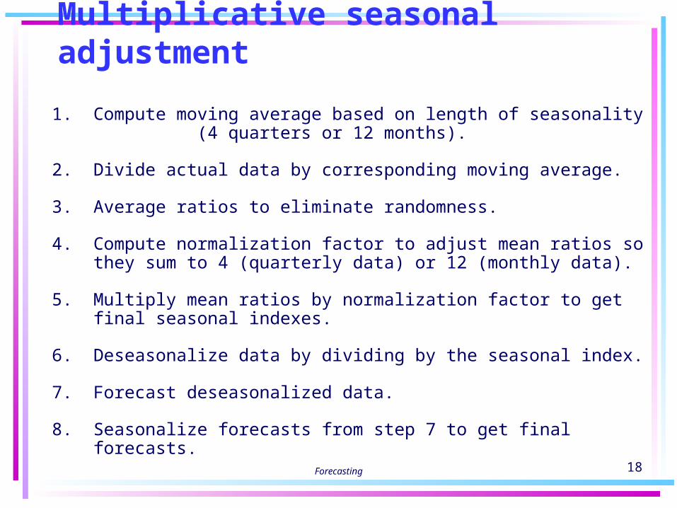
Multiplicative seasonal adjustment
1. Compute moving average based on length of seasonality (4 quarters or 12 months).
2. Divide actual data by corresponding moving average.
3. Average ratios to eliminate randomness.
4. Compute normalization factor to adjust mean ratios so they sum to 4 (quarterly data) or 12 (monthly data).
5. Multiply mean ratios by normalization factor to get final seasonal indexes.
6. Deseasonalize data by dividing by the seasonal index.
7. Forecast deseasonalized data.
8. Seasonalize forecasts from step 7 to get final forecasts.

Forecasting 19
Additive seasonality
The seasonal index is the expected difference between actual data and the average for the year.
Actual data - Index = Seasonally adjusted data
Seasonally adjusted data + Index = Actual data
Additmon.xls

Forecasting 20
Additive seasonal adjustment1. Compute moving average based on length of seasonality
(4 quarters or 12 months).
2. Compute differences: Actual data - moving average.
3. Average differences to eliminate randomness.
4. Compute normalization factor to adjust mean differences so they sum to zero.
5. Compute final indexes: Mean difference – normalization factor.
6. Deseasonalize data: Actual data – seasonal index.
7. Forecast deseasonalized data.
8. Seasonalize forecasts from step 7 to get final forecasts.

Forecasting 21
Forecasting simulations
Dynamic simulation● Short-range (one-step-ahead) forecasting test● Use data in fit periods to select model● During forecast periods:
1. Make one forecast.2. Observe error.3. Adjust model.4. Go to 1.
Static simulation● Long-range forecasting test● Use data in fit periods to select model● Make all forecasts at once
Forecasting 22
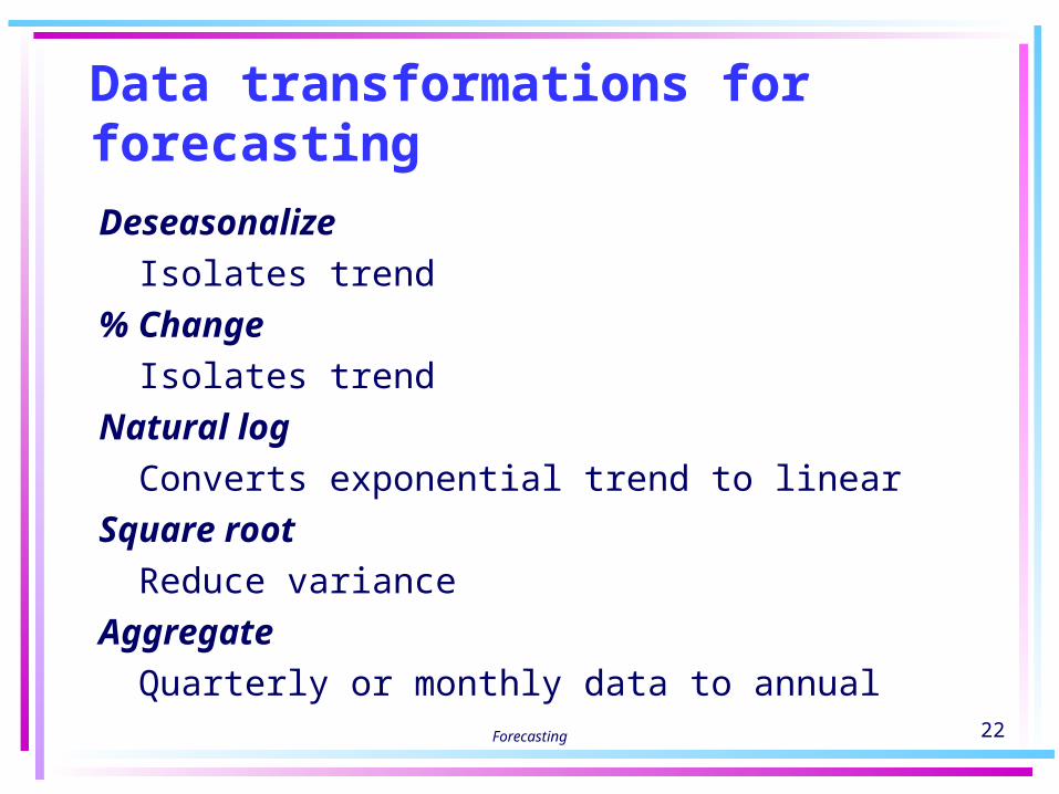
Data transformations for forecasting
DeseasonalizeIsolates trend
% ChangeIsolates trend
Natural logConverts exponential trend to linear
Square rootReduce variance
AggregateQuarterly or monthly data to annual

Forecasting 23
Forecasting management
Organize for forecasting● Pinpoint responsibility● Only one corporate forecast● Separate forecasting and planning
Monitor accuracy● Choose a standard measure● Keep a track record● Benchmark● Hold performance reviews
Scrub the data● Adjust outliers● Throw out unique data

Forecasting 24
Forecasting management (cont.)
Compare alternative forecasts● Top-down vs. bottom up● Monthly vs. quarterly data● Deseasonalized vs. raw data● Percent change data● Time series forecasts● Regression forecasts
Simulate forecasting● One-step-ahead● Long-range
Estimate confidence limits● What is the range of forecast errors in past?