forecasting and time series analysis using the sca …this edition of forecasting and time series...
TRANSCRIPT

FORECASTING AND TIME SERIES ANALYSIS USING THE SCA STATISTICAL SYSTEM
VOLUME 1
Box-Jenkins ARIMA Modeling Intervention Analysis
Transfer Function Modeling Outlier Detection and Adjustment
Exponential Smoothing Related Univariate Methods
by
Lon-Mu Liu
Gregory B. Hudak
in collaboration with
George E. P. Box Mervin E. Muller George C. Tiao
This manual is published by
Scientific Computing Associates Corp. 913 West Van Buren Street, Suite 3H
Chicago, Illinois 60607-3528 U.S.A.
Copyright Scientific Computing Associates Corp., 1992-1994

PREFACE
This edition of Forecasting and Time Series Analysis Using the SCA Statistical System
initiates the replacement process of the document entitled The SCA Statistical System: Reference Manual for Forecasting and Time Series Analysis (May 1986). When the replacement process is complete, the older manual will have been completely replaced in both scope and style by a two volume set.
This manual is Volume I of the set. It encompasses topics related to the capabilities of the UTS Module and the Extended UTS Module of the SCA Statistical System. Hence the contents of this manual replace Chapters 1, 2, 3, 7, and 8 of the 1986 manual entirely. Chapters 4, 5, and 6 of the 1986 manual are still valid until the release of Volume II of the new set. In addition, information related to the spectral analysis capabilities of the SCA System may be found in SCA Working Paper 115.
As noted above, this manual is a complete revision of parts of the 1986 manual. Chapter 4, “Linear Regression Analysis”, replaces Chapter 8 of the previous manual. The chapter is a modified version of the regression chapter of the document The SCA Statistical System: Reference Manual for General Statistical Analysis. Chapters 5 through 8 are a detailed replacement of Chapter 3 of the 1986 document. Information related to the modeling and forecasting of univariate time series is divided into chapters on “Box-Jenkins ARIMA Modeling and Forecasting” (Chapter 5), “Intervention Analysis” (Chapter 6), “Outlier Detection and Adjustment” (Chapter 7), and “Transfer Function Modeling” (Chapter 8). Chapter 7 of this manual contains material not present in the 1986 edition. This new chapter includes much of the current information of the burgeoning research and activities associated with outlier detection, adjustment and estimation. Chapter 9, “Forecasting Using General Exponential Smoothing”, is an upgrade of Chapter 7 of the earlier manual. Examples have been added to illustrate all supported smoothing methods.
Almost all material of the above chapters is presented in a “data analysis” form. That is, SCA capabilities, commands, and output are presented within the context of a data analysis. Many concepts related to data analysis are reviewed and explained. Examples have been chosen to demonstrate the use of the SCA System, and to provide some insights or guidelines for an analysis.
Within chapters, information regarding specific capabilities and features of the SCA System are presented from those most frequently used to those that are less commonly employed. All detailed information regarding the command structure of the SCA System is presented at the end of each chapter.
This manual is designed to be self-contained. Chapter 1 of this document provides complete information on the contents of all available SCA software products and where specific information on various SCA System capabilities can be found. Chapter 2 provides an overview of the command language of the SCA System. Chapter 3 summarizes useful plotting features for modeling time series. Five appendices provide information on the basic

use of analytic statements; data generation, editing and creation; SCA macro procedures; and selected utility commands. More complete information on SCA commands can be found in The SCA Statistical System: Reference Manual for Fundamental Capabilities.
Acknowledgements
The SCA Statistical System was designed and developed by Lon-Mu Liu with the assistance of the SCA programming staff. Acknowledgements specific to capabilities described in other reference manuals are found in selected chapters. We are particularly grateful to Chung Chen of Syracuse University and George C. Tiao of The University of Chicago for their contributions related to outlier detection and adjustment, and Ruey S. Tsay of The University of Chicago for his program related to the EACF paragraph. Bovas Abraham of The University of Waterloo and Johannes Ledolter of The University of Iowa contributed greatly to the development of the GFORECAST paragraph and providing a review of our 1986 chapter on exponential smoothing. Houston H. Stokes of The University of Illinois has constantly rendered his programming expertise in the development of the SCA System. We are also grateful to Ki-Kan Chan and Alan Montgomery for their programming and testing efforts regarding SCA products on various computer platforms.
This manual was prepared by Lon-Mu Liu, The University of Illinois at Chicago, and Gregory Hudak, Scientific Computing Associates Corporation. We thank George E.P. Box, George C. Tiao, and Mervin E. Muller, for their valuable comments and suggestions related to various aspects of the SCA System. We are indebted to the tireless efforts of Ching-Te Liu in the entry and editing of all chapters of this manual. This volume could not have been completed without her complete dedication to this project.
Scientific Computing Associates Corporation February, 1992

CHAPTER 1
INTRODUCTION
The Forecasting and Modeling Package of the SCA Statistical System is comprised of
four products. These products are:
UTS: Univariate time series analysis and forecasting using Box-Jenkins ARIMA, intervention and transfer function models. This product also includes forecasting capabilities using general exponential smoothing methods.
Extended UTS: Univariate time series analysis and forecasting with automatic outlier detection and adjustment, as well as analysis and forecasting of time series containing missing data
MTS: Multivariate time series analysis and forecasting using vector ARMA models
ECON/M: Econometric modeling and forecasting using simultaneous transfer function models. This module also provides the seasonal adjustment procedures X-11, X-11-ARIMA, and a model-based canonical decomposition method.
This manual describes the capabilities of the SCA UTS and Extended UTS products of the SCA System. Capabilities described in this manual (and chapters containing them) include:
Plotting data: (Chapter 3)
Plots of one or more variables over time, and scatter plots of two or more variables.
Linear regression analysis: (Chapter 4)
Multiple linear regression analysis, the effect of serial correlation, and dynamic regression
Box-Jenkins ARIMA modeling: (Chapter 10)
Time series analysis and forecasting of a single series using Box-Jenkins ARIMA models. Data simulation is also discussed.
Intervention analysis: (Chapter 6)
Modeling and analysis of the effects of known external events on a single time series.
Outlier detection and adjustment: (Chapter 7)
Descriptions of outliers and methods for outlier detection and adjustment. Also included are forecasting in the presence of outliers and modeling a time series that contains missing observations.

Transfer function modeling: (Chapter 8)
Modeling a response variable (series) in the presence of one or more explanatory variables and a serially correlated disturbance term. Also presented are special cases of transfer function models; applications of transfer function modeling for handling the effects of trading days and moving holidays; and data simulation.
General exponential smoothing forecasting: (Chapter 9)
Forecasting a nonseasonal series using single and double exponential smoothing, or Holt's two parameter method. Forecasting a seasonal series using Winters additive or multiplicative methods, seasonal indicators and harmonic functions. Relationships to Box-Jenkins ARIMA models are also discussed.
Analytic functions and matrix operations: (Appendix A)
Analytic functions and matrix operations that supplement the SCA System's statistical capabilities.
Data generation: (Appendix B)
User specified data generation, editing and other data manipulation of variables that are not necessarily time dependent.
Time series data generation: (Appendix C)
User specified data generation and editing of time series data.
Macro procedures: (Appendix D)
Creation and use of sequences of SCA statements to either perform SCA data analyses or to augment SCA capabilities.
Utility information: (Appendix E)
Output saving and review, management of files, internal workspace (memory), and other utility related tasks of an SCA session.
Most of the information contained in the Appendices is condensed from that described in The SCA Statistical System: Reference Manual for Fundamental Capabilities and The SCA Statistical System: Reference Manual for General Statistical Analysis. Selected information regarding the basic use of the SCA System and data entry can be found in Chapter 2. The information in Chapter 2 and the Appendices are designed to provide self-contained documentation for the use of the SCA-UTS and Extended UTS products.
Whenever possible, material in this manual is presented in a “data analysis” form. That is, SCA System capabilities, commands, and output are usually presented within the context of a data analysis. Examples have been chosen to both demonstrate the use of the SCA System and to provide some broad guidelines for forecasting and time series analysis. One

INTRODUCTION 1.3
key reference and source of examples in this manual is the text Time Series Analysis: Forecasting and Control by Box and Jenkins (1970). This text contains many important concepts and properties of forecasting and time series analysis.
1.1 Forecasting and Time Series Analysis for Business, Industry and the Public Sector
In recent years, business, industry and the public sector have coped with the two-fold problem of providing quality goods and services while contending with limited or shrinking resources. Statistical methods can provide broad and effective means to address this problem.
In particular, accurate forecasts are necessary for such diverse activities as capital budgeting, sales forecasting, market research, financial planning, and inventory planning and control. Statistical modeling and analyses are important for such activities as understanding the structure of a process, price analyses, and impact (or regulatory) analyses. The overall decision making process can benefit greatly from accurate forecasting and modeling tools.
Processes of interest are usually characterized by the response measured for one or more process attributes. In addition to such responses, we may also have recorded the values or operating conditions of possibly related (explanatory) variables. Statistical methods are often used to construct models that employ some, or all, of this information. Box (1979a) has noted that “Models ... are never true, but fortunately it is only necessary that they be useful”.
One key element in statistical model building is how to deal with variation. Whenever we attempt to learn about a process, we are faced with dealing with the natural variation that is present in it. Such variation is confounded with the variation that occurs in simply determining (measuring) the values of all variables related to the model. In the case of data that are gathered according to some time order, we also must account for the time related correlation that is present in recorded values. Time series methods have proven useful for the characterization and forecasting of such time dependent processes.
1.2 Iterative Model Building and the SCA Statistical System
Box has often noted (e.g., 1974, 1976, 1979a, 1979b, and 1983) that statistical analyses or model building are most effective when an inductive-deductive approach is used. Observation and basic knowledge leads to the postulation of a theory or model. The theory or model is tried and the results are reviewed to provide insight for the modification or correction of the theory or model as necessary. The process continues until a satisfactory result is obtained. Within the model building process, this is realized as the cycle of initial model identification (or specification), model estimation, and diagnostic checking.
With the advent of high-speed computers, model building can be automated by incorporating sophisticated rules for decision making. Box (1984) notes that he and Gwilym Jenkins “thought that it was particularly important not to try to make the model-building process automatic and entirely controlled by the computer, but to ensure that the human brain intervened and controlled, particularly at the identification and the diagnostic checking/model

modification stages. Subsequent experience has (he contends) demonstrated the rightness of this idea”. This dynamic inductive-deductive approach to model building and analysis is greatly facilitated by the flexibility in the SCA Statistical System allowing its capabilities to be blended in any logical order for such purposes. The SCA System also provides important automated capabilities for model estimation and modification.
1.3 The SCA System
The Scientific Computing Associates Corporation (SCA) provides several self-contained modules in its statistical software system. At present, the SCA Statistical System includes the SCA-UTS module for univariate time series analysis and forecasting, the Extended UTS module for univariate time series analysis and forecasting with automatic outlier detection and adjustment, the SCA-MTS module for multivariate time series analysis and forecasting, the SCA-ECON/M module for econometric modeling and forecasting, the SCA-GSA module for general statistical analysis, and the SCA-QPI module for industrial quality and process improvement. The capabilities of other modules are discussed in other documents. In addition to its own unique capabilities, each module of the SCA System also contains a complete set of SCA fundamental capabilities, including data input and output, analytic functions and matrix operations, data manipulation and editing, histograms and plots, macro procedures and other utility capabilities. Details regarding these capabilities are also described in The SCA Statistical System: Reference Manual for Fundamental Capabilities.
The modules described above are available as components in three statistical packages offered by SCA. These packages and their component modules are:
General Application Package: GSA
Forecasting and Modeling Package: UTS, Extended UTS, MTS, ECON/M and GSA
Quality Improvement Package: QPI and GSA
In addition to the statistical modules described above, SCA provides software for employing windows and graphics, the SCA Windows/Graphics Package. This package provides an innovative means to integrate the computing power of mainframe computers and workstations with the user-friendly features and high-resolution graphics capabilities available on personal computers. The SCA Windows/Graphics Package provides for:
• A window environment for the SCA System, • Menus to access all SCA capabilities, • Convenient on-line help for SCA capabilities, and • Two-way data transfer between mainframe computers and a PC.
A component of the SCA Windows/Graphics Package is the PC product SCAGRAF.
SCAGRAF is a Microsoft Windows application product providing such statistical and graphical features as:

INTRODUCTION 1.5
• Single (and multiple) time series plots and scatter plots, • Box-Cox transformations, • Time series model identification tools, • Forecast and outlier plots, • Quality control charts, and • Contour plots,
Many of the figures in this document were generated using SCAGRAF.
REFERENCES Box, G.E.P. (1974). “Statistics and the Environment”. Journal of the Washington Academy
of Science, 64: 52-59.
Box, G.E.P. (1976). “Science and Statistics”. Journal of the American Statistical Association, 71: 791-799.
Box, G.E.P. (1979a). “Some Problems of Statistics and Everyday Life”. Journal of the American Statistical Association, 74: 1-4.
Box, G.E.P. (1979b). “Robustness in the Strategy of Scientific Model Building”. Robustness in Statistics (ed. by R.L. Launer and G.N. Wilkenson): 201-236. New York: Academic Press.
Box, G.E.P. (1983). “An Apology for Ecumenism in Statistics”. Scientific Inference, Data Analysis, and Robustness (ed. by G.E.P. Box, Tom Leonard and Chien-Fu Wu): 51-84. New York: Academic Press.
Box, G.E.P. (1984). “Gwilym Jenkins, Experimental Design and Time Series”. The Collected Works of George E.P. Box (ed. by George C. Tiao). Belmont, CA: Wadsworth.
Box, G.E.P. and Jenkins, G.M. (1970). Time Series Analysis: Forecasting and Control. San Francisco: Holden-Day. (Revised edition published 1976).


CHAPTER 2
SYSTEM BASICS
Every software system has its own vocabulary and language to put user’s “words” into
action. This chapter provides the basics of the SCA command language and the use of the SCA System. In addition, information concerning the entry of data to the SCA System is also provided. More complete information can be found in The SCA Statistical System: Reference Manual for Fundamental Capabilities.
2.1 Getting Started
The SCA System is a command driven system. That is, the System responds to user instructions (commands) rather than to user chosen options from a menu. When the SCA System is used through the SCA Windows/Graphics Package, a Command Builder creates necessary commands from menu selections. In this manner, the SCA System has the same command language at all computing levels. All command lines must be followed by a carriage return. For easier reading in the remainder of this manual, we shall not explicitly display ‘<cr>’ (carriage return) when presenting command lines. However, all command lines of the SCA System are preceded with the symbols ‘-- >’ as a means to indicate a line entered by the user. The symbols ‘-- >’ themselves should not be entered.
Mainframe and workstation computers
To access the SCA System on a mainframe computer, we enter
SCA ( or sca )
If this command does not invoke the System, a local computer consultant should be contacted regarding the appropriate command. It is possible a computing center may have installed the SCA System under a different command name.
Personal computers
The SCA System is also available for use on personal computers having a DOS, OS/2 or Macintosh operating system. Within the DOS or OS/2 environment, we first enter the subdirectory in which the SCA System was installed. The PC SCA System installation guide advises that the subdirectory be named SCA for DOS operating systems and OS2-SCA for OS/2 operating system. Thus enter
CD \SCA (or CD \OS2-SCA).
To invoke the SCA System in this directory, enter

2.2 SYSTEM BASICS
SCA
To invoke the SCA System on Macintosh, we can simply double click the SCA icon from the folder in which it is stored. The icon should be created when the SCA System is installed.
System heading and prompt
When the SCA System is appropriately invoked, a set of short descriptive information appears. For example, the heading at an IBM/CMS mainframe site will be something like
* * * * * COMPUTER SERIAL NUMBER ( 172353 / 12345 ) * * * * * THE SCA STATISTICAL SYSTEM ( RELEASE IV.3 ) SCA PRODUCT IDENTIFICATION: GSA, UTS, MTS, ECON/M & QPI HOST COMPUTER OPERATING SYSTEM: IBM/CMS COPYRIGHT 1985 - 1990, SCIENTIFIC COMPUTING ASSOCIATES. ALL RIGHTS RESERVED RELEASED DATE: 3/ 1/90 SIZE OF WORKSPACE IS 50000 SINGLE PRECISION WORDS DATE -- 11/30/90 TIME -- 10:10:43 --
This set of information includes SCA release version, product names, host computer and operating system, and workspace (memory) size. The heading information is followed by a double dash, ‘--‘. The double dash is a prompt issued by the SCA System. This indicates we can now enter an SCA command.
When the SCA System on a mainframe or workstation computer is invoked through the SCA Windows/Graphics Package (see the related document SCA Windows/Graphics Package User's Guide for more information), the following windows appear on the PC screen.

SYSTEM BASICS 2.3
The heading information and subsequent SCA output are contained in the output wind
Creating a larger workspace environment
ow SCAOUTP.OTP. SCA commands are entered in the SCA command window, SCAHIST.CMD, or are generated from menu selections through the SCA Command Builder. The command history (i.e., the set of all SCA commands entered) of the SCA session is maintained in this window.
We can designate a larger workspace (memory) size for an SCA session when we invok
The designation of a larger workspace varies somewhat between computers and opera
SCA n
here n is an integer, will allocate nK words of memory for the session. The instruction is
e the SCA System. This is a useful feature when we are dealing with larger data sets or complex computations. The amount of workspace that can be designated may be restricted due to local computer installation constraints or an SCA System constraint, depending on the subscription level. The maximum workspace size for the SCA System on personal computers varies between 30K and 35K words (1K words = 1000 words), while the maximum workspace for the SCA System on mainframe and workstation computers usually does not have a specific limit.
ting systems. For most operating systems, invoking the SCA System with
wdifferent for IBM TSO and CMS operating systems where we must use either SCA SIZE(n) (for an IBM TSO operating system)

2.4 SYSTEM BASICS
or SCA SIZE n (for an IBM CMS operating system)
none of the above instructions affect the workspace size, it is necessary to check with a
2.2 General Syntax of System Commands
Once we are in the SCA System, we have begun an SCA session. All SCA commands withi
Each statement is entered after the ‘--‘ prompt. We can use blanks freely in a statement to spa
Iflocal computer consultant to determine what to do.
n a session are the same across all computer types. These commands are also called “statements”.
ce words, but blanks cannot be used within names or numbers. Usually command lines are limited to 72 spaces and most commands can be written in one line. If we need to continue to another line, the current line must be ended with the character ‘@’. We refer to the symbol ‘@’ as the continuation character. It must be the last non-blank character of any line being continued. It cannot be used as a hyphenation character. That is, words and numbers cannot be divided with ‘@’. The SCA System processes a command whenever a line is entered that does not end with ‘@’.
Analytic statements
There are two types of statements that we can use during an SCA session, analytic or “Eng
v = e
where “e” is an expression involving a combination of operators and variable names (the labels
LNY = LN(Y)
will take the natural logarithm of the data currently being held in the variable Y and store
TEMP = INV(A) # B
will multiply the matrix B by the inverse of the matrix A (i.e., ), then store the result
A complete list of SCA analytic functions and matrix operators can be found in Appe
lish-like”. Analytic statements are used for most vector and matrix operations or manipulations. These statements have the general form
used to retain data in the SCA workspace); and “v” is a variable name (label) that will be used to hold results. For example,
the result into the variable LNY. The statement
1A B−
s into the variable TEMP.
ndix A. Some examples are also provided. A more detailed discussion regarding analytic statements can be found in The SCA System: Reference Manual for Fundamental Capabilities.

SYSTEM BASICS 2.5
English-like statements
English-like statements (or paragraphs) are used to accomplish most operations in an SCA session. These statements consist of a paragraph name that can be followed by one or
For example,
ph name is PRINT and the modifying sentence is VARIABLE IS GROWTH. Here the function of the statement is implicit in the paragraph
a e. odifying sentence is sufficient for the execution f the command.
be ended with a period if another sentence is to follow. Each line within the paragraph, except for the last line, must have the continuation character (‘@’) as its last chara
An optional sentence is used only if we wish to change a default condition. A sentence is required if no default condition (or value) exists. If we omit any required sente
PLOT VARIABLES ARE TAX, INCOME
200 data pairs (see Chapter 3 for more information on scatter plots). If we enter
PLOT VARIABLES ARE TAX, INCOME. SPAN IS 1,150
using only the first 150 pairs of data. The entences VARIABLES and SPAN must be separated by a period. If we only enter
PLOT SPAN IS 1, 150
BLES is required sentence.
more modifying sentences.
PRINT VARIABLE IS GROWTH is an English-like statement. The paragra
n m Information contained in the single mo
The first word of a paragraph must be a valid paragraph name. This name is then followed by any number of modifying sentences. Sentences have no specific order of entry. A sentence must
cter.
Modifying sentences fall into two categories: required and optional. A sentence is optional if there is a default condition (or value) that can be used during the execution of the paragraph.
nce, the System will issue prompts requesting the information omitted.
For example, suppose there are two variables in the SCA workspace, TAX and INCOME, each containing 200 values. If we enter
then the System will produce a scatter plot using all
then the System will produce a scatter plots then the System will prompt us for the variables to be used in the plot, since VARIAa
Most frequently used required sentence
For our convenience, the subject and verb of the ``most frequently used sentence'' of a paragraph can be omitted provided the sentence is the first sentence used after the paragraph

2.6 SYSTEM BASICS
name. For example, the VARIABLE sentence is the most frequently used sentence of both the PRINT and PLOT paragraphs. If we desire, we can omit the words VARIABLES ARE in these
IS GROWTH
1,150
the SCA System in the same fashion as the statement
. SPAN IS 1, 150
urs. The System would interpret TAX as the first three letters of a ntence name and not
paragraphs. That is, the statement
PRINT GROWTH is equivalent to the statement
PRINT VARIABLE The statement PLOT TAX, INCOME. SPAN IS is processed by PLOT VARIABLES ARE TAX, INCOME Note that if the statement PLOT SPAN IS 1, 150. TAX, INCOME is entered, then an error occse as variable information. Very often, the “most frequently used
The portion of the “most frequently sed sentence” that can be omitted is highlighted in the syntax description for every paragraph
To illustrate the types of commands and using the SCA System, we will examine some data taken from the text Statistics for Experimenters by Box, Hunter and Hunter (1978). The
h the growth rate (in coded units) of experimental rats and the amount (in grams) of a dietary substance fed to the rats.
sentence” is the only sentence specified in a paragraph.uof the SCA System.
2.3 An Example
data, s own below, are

SYSTEM BASICS 2.7
Growth rate Dietary supplement 73 10 78 10 85 15 90 20 91 20 87 25 86 25 91 25 75 30 65 35
We first want to transmit (or enter) data into the System's workspace (memory). There are many ways in which data can be entered. Complete information on the entry of data into the SCA workspace is provided in Chapter 3 of The SCA Statistical System: Reference Manual for Fundamental Capabilities. A summary of some frequently used methods for data entry is given in Section 10 of this Chapter. In this example we will enter both columns of data directly from the terminal. To enter the growth rate data we can enter
-->INPUT GROWTH Note that the use of ‘-->’ in this document denotes a line we are entering (and should not be typed). We also must press the carriage return key to end our entry. We have informed the System that we will be transmitting data to it and want it retained in the System's workspace (memory) under the label GROWTH. Any valid name (see Section 2.4) can be used as a label for a variable. GROWTH has been chosen since this label is well suited to designate the data. The System responds with
READY FOR DATA INPUT
The ‘--‘ prompt is not displayed because the System is not expecting any sort of instruction, just data. We can enter the data on one line by entering: -->73 78 85 90 91 87 86 91 75 65 In order to tell the System that we are finished entering data for GROWTH, we now type
-->END OF DATA The System responds with
GROWTH , A 10 BY 1 VARIABLE, IS STORED IN THE WORKSPACE
Now we enter the dietary supplement data and retain it in the workspace under the label
DIET.

2.8 SYSTEM BASICS
-->INPUT DIET
READY FOR DATA INPUT
-->10 10 15 20 20 25 25 25 30 35 -->END OF DATA
DIET , A 10 BY 1 VARIABLE, IS STORED IN THE WORKSPACE
Before we continue, we can display the data that has been transmitted. We do this by
entering
-->PRINT GROWTH, DIET
GROWTH IS A 10 BY 1 VARIABLE DIET IS A 10 BY 1 VARIABLE VARIABLE GROWTH DIET COLUMN--> 1 1 ROW 1 73.000 10.000 2 78.000 10.000 3 85.000 15.000 4 90.000 20.000 5 91.000 20.000 6 87.000 25.000 7 86.000 25.000 8 91.000 25.000 9 75.000 30.000 10 65.000 35.000
To get an idea of how growth rate and dietary supplement are related, we display a
scatter plot (see Chapter 3) by entering
-->PLOT GROWTH, DIET
91.80 + * * I * I I 2 I * 82.80 + I G I R I * O I * W 73.80 + * T I H I I I 64.80 + * -+---------+---------+---------+---------+ 9.10 16.10 23.10 30.10 37.10 DIET

SYSTEM BASICS 2.9
We observe that the effect of the dietary supplement on the growth rate increases to a peak level, then falls off. As a result we may wish to use regression analysis (see Chapter 4) to estimate the model.
20 1 2Y b b X b X error= + + +
where Y is the growth rate and X is the amount of dietary supplement. We do not have the quadratic term, X at present, but we can create it by using an analytic statement (see Appendix A). One means to create X is to enter
2
2
-->DIET2 = DIET**2 The data generated by this command are retained in the workspace under the label DIET2. We are now ready for a regression analysis. We can fit the model above by entering -->REGRESS GROWTH, DIET, DIET2
The output generated from this command is suppressed at this time. Other options are available to us within the REGRESS paragraph, for example diagnostic checking, retaining calculated values and methods of fitting (see Chapter 4 for more information).
2.4 Names and Abbreviations
All data and models are stored in the SCA workspace (memory). We are required to provide names for all data and models that we place in the workspace. Other names used in an SCA session (i.e., paragraph and sentence names) are a part of the System's command language.
The names we specify for data or models can be of any length, although only the first eight characters are interpreted by the System. The first character of a name (label) must be a letter. The other characters may be letters, numbers or the underscore symbol, ‘_’. Blanks cannot be used as part of a name. Examples of valid names that we may specify are:
X, XDATA, X_DATA, X1, SERIES1, SERIES_1, DATASET1,
XDCDDEA, S33E45, F55XX_2, INFORMATION_FOR_SERIES_1 Examples of some invalid names are: 1X (the first character is not a letter)
X DATA (blanks are not permitted)
X0DATA (the special character ‘-‘, hyphen, is not permitted)

2.10 SYSTEM BASICS
Abbreviation rules
All names used in an SCA session can be abbreviated. Names and labels that we specify are identified by the SCA System by their first eight (8) characters only. Hence the name
INFORMATION_FOR_SERIES_1 is interpreted by the SCA System as INFORMAT. The remaining characters are not maintained in memory, but may be used for readability. Thus, the name INFORMATION_FOR_SERIES_2 is also interpreted by the System as INFORMAT. As a result, if we transmit data sequentially using these two names then all data first stored in the workspace under the label INFORMAT would be overwritten by the latter.
All sentence names are uniquely defined by their first three characters. Paragraph names are likewise defined, with a few exceptions due to name multiplicity (e.g., CORNER and CORRELATION). These names may be reduced to the first four characters. For example, the System internally interprets the statement
-->PLOT VARIABLES ARE WITHHOLDING, INCOME. @ --> SPAN IS 1, 30. as -->PLO VAR ARE WITHHOLD, INCOME. SPA IS 1, 30.
2.5 Reserved Words and Symbols
Certain words and symbols have special meaning to the SCA System. They are summarized below and should only be used in their special context. More details can be found in The SCA Statistical System: Reference Manual for Fundamental Capabilities.
(1) FOR, TO, BY and $ are used to specify an implied list of arguments.
(2) The apostrophe ( ‘) is used in the identification of character strings.
(3) @ is a continuation symbol. It can also be used within macro procedures. (4) -- is interpreted as an in-line comment when it is specified by the user. (5) . specifies either a decimal point or a period.
(6) IS, ARE, IN, and ON are used as verbs within SCA sentences provided they immediately follow a sentence name. Otherwise, they are interpreted as variable names.

SYSTEM BASICS 2.11
(7) The exclamation mark ! is used to cancel a statement when it appears as the last
character of a statement.
2.6 Obtaining On-Line Help
The SCA System provides interactive on-line help on the capabilities and syntax of statements of the System. To obtain help information, enter the statement
-->HELP More complete information is then provided. To obtain information on a specific SCA paragraph, enter -->HELP paragraph-name To terminate a help session on mainframe computers, enter QUIT. To terminate the help session on a PC, press the ESC key. The System will then display the prompt ‘--‘ and the user will be at that position in an SCA session where help was requested. (If the DOS or OS/2 prompt ‘C>’ appears in the PC environment, enter the command QUIT.)
2.7 Responding to Prompts
Whenever a required sentence of a paragraph is either omitted or incomplete, the System will prompt for information it requires. When the System issues prompts, it only wants a direct response to its inquiries. For example, if we enter the statement
-->PLOT rather than the statement -->PLOT TAX, INCOME then the System will issue a prompt for the variable names omitted. Although the sentence that has been omitted is VARIABLES ARE TAX, INCOME, the System does not want the entry of the text for this full sentence. In issuing a prompt, the System “knows” what sentence has been omitted, and it only wants the information omitted, i.e., TAX and INCOME. The response we need to provide is simply -->TAX, INCOME
Prompts will continue until the System has all the necessary information it requires to proceed with the specified paragraph. If we wish to terminate the prompting session, we can do so by entering the instruction QUIT. In addition to terminating the prompting session, the QUIT command will also abort the execution of the paragraph.

2.12 SYSTEM BASICS
2.8 Panic Buttons
Occasionally, we may want to stop what is currently happening and get back to the basic command level (‘--‘). The following are useful “panic” buttons:
(1) CTRL-C The execution of any paragraph can be terminated by simultaneously holding down the CTRL and C keys (or Break key for IBM MVS and IBM CMS operating systems). Output may not stop immediately as some output may already have been sent to a print buffer. In the IBM MVS and IBM CMS environments, be careful not to enter the Break key continuously as three successive entries of the Break key will terminate the SCA session.
(2) QUIT The instruction QUIT will terminate any prompting session. This will also
terminate the execution of the specified command.
(3) ! The exclamation mark will cancel any statement, provided it is the last character of the statement. For example, suppose we enter the lines
-->PLOT TEX, INCOME. @ --> SPAN IS 1, 30
If we realize we have misspelled TAX as TEX before we transmit the second line, we can cancel the entire command by ending the second line with ‘! ‘.
2.9 Ending an SCA Session
To exit from an SCA session, enter the command -->STOP
2.10 Entering Data
There are many ways in which data can be transmitted to the SCA System. This section presents examples of the most common ways to enter data. The SCA paragraph INPUT may be used to transmit any data to the SCA System. Other paragraphs, BINPUT and FINPUT, are also available for special types of data.
2.10.1 Entering data from the terminal
We will first demonstrate how to enter data directly from a terminal during an SCA session. We will use the two data sets presented in Section 2.3 of this Chapter, growth rate and dietary supplement. The data sets are small enough that we may consider entering the data directly from the keyboard. Previously, all the data of one variable were entered, then all the data of the other were entered. This is called variable by variable data entry.

SYSTEM BASICS 2.13
Alternatively, we could choose to enter both variables at the same time by entering the first pair of data, then the second, and so on. This is called case by case data entry.
Entering data of a single variable
To enter the data for growth rate in a variable by variable fashion and store the data in the SCA workspace under the label GROWTH, enter
-->INPUT GROWTH This is equivalent to the statement -->INPUT VARIABLE IS GROWTH in which the complete VARIABLE sentence is specified. The System responds with
READY FOR DATA INPUT
We now can enter data using free format (that is, data are separated by one or more blanks). We can enter all data on the same line, for example -->73 78 85 90 91 87 86 91 75 65 or -->73 78 85 90 91 87 86 91 75 65 We can also enter one data value per line, for example -->73 --> 78 --> 85 --> 90 --> 91 -->87 --> 86 -->91 --> 75 --> 65 or we could enter the data on multiple lines -->73 78 85 --> 90 91 -->87 86 91 75 65

2.14 SYSTEM BASICS
As soon as we are through entering data, we enter -->END OF DATA (or -->END) This completes the data entry for the variable GROWTH. The System will then respond with the message
GROWTH , A 10 BY 1 VARIABLE, IS STORED IN THE WORKSPACE
Entering data for more than one variable
Instead of entering the two data sets in a variable by variable fashion, we could transmit both data sets simultaneously (i.e., in a case by case fashion) by entering
-->INPUT GROWTH, DIET After the System prompt for data, we enter the ten cases of data using free format. Each case must be on a new line (record). This is, we enter -->73 10 -->78 10 -->85 15 -->90 20 -->91 20 -->87 25 -->86 25 -->91 25 -->75 30 -->65 35 -->END OF DATA The System will then respond with the message
GROWTH , A 10 BY 1 VARIABLE, IS STORED IN THE WORKSPACE DIET , A 10 BY 1 VARIABLE, IS STORED IN THE WORKSPACE
Each case (or record, or row) is transmitted in free format, so that the alignment shown above is arbitrary. Each line of data can be written in any convenient form.
2.10.2 Options related to the INPUT paragraph
When we enter data from the terminal, the only required sentence associated with the INPUT paragraph is the VARIABLES sentence. Unless informed otherwise, the SCA System assumes the data of any variable to be in free format, be a single column vector, be of single precision, and have no missing values. If we need to change any of these default conditions then an appropriate modifying sentence must be added.

SYSTEM BASICS 2.15
Entering a matrix of data
When we transmit a matrix of data to the SCA System, we need to indicate the number of columns (NCOL) in the matrix. The number of rows is determined from the number of rows of data entered. For example, suppose the growth rate data was actually a matrix consisting of two columns of data. The value in the first column is the growth rate in week 1 and the value in the second column is the growth rate in week 2. To enter the GROWTH data as a 10 x 2 matrix, we may enter
-->INPUT GROWTH. NCOL ARE 2. and now enter data in a case by case fashion after the System prompt, for example -->73 70 -->78 81 -->85 86 -->90 87 -->91 92 -->87 86 -->86 87 -->91 89 -->75 79 -->65 62 -->END OF DATA
The default value of NCOL for each variable is 1. If NCOL is changed from 1 for any variable, then data must be transmitted in a case by case fashion as above. For example, if we enter
-->INPUT XVECTOR, YMATRIX. NCOL ARE 1, 3. and enter the following data -->1 2 3 4 5 6 7 8 -->8 7 6 5 4 3 2 1 -->0 1 1 2 2 3 3 3 -->END OF DATA Then XVECTOR will be a 3 x 1 vector consisting of the values 1, 8, and 0; and YMATRIX will be the 3 x 3 matrix 2 3 4 7 6 5 1 1 2 All values after the 1 + 3 = 4th column of any row are ignored by the System.

2.16 SYSTEM BASICS
Entering non-numeric data, the PRECISION sentence
The SCA System assumes that all data transmitted are single precision numeric data. To alter this default, we need to employ the PRECISION sentence. For example, suppose dietary data to be transmitted consist of the type of diet the rat was fed, A, B or C (i.e., character data) as well as the above two weeks worth of growth data. We can enter the statement
-->INPUT GROWTH, DIET. NCOLS ARE 2, 1. @ --> PRECISIONS ARE SINGLE, CHARACTER Here two modifying sentences, NCOL and PRECISIONS, are used. NCOL specifies that the variable GROWTH has two columns of data and that DIET has one column of data. The PRECISION sentence is used to specify that DIET consists of character information. Since the default condition of the PRECISION sentence was changed for one variable (DIET), we need to specify the appropriate modifier for all variables of the sentence. Also note that since we were unable to write the INPUT statement entirely on one line, we used the continuation symbol, ‘@’.
2.10.3 Entering data from a file
In practice, we do not always enter data directly from a terminal. Often data exists on an external “flat file”. A “flat file” is one that can be created or edited by a text editor. Flat files generally contain only one data set, or one set of case by case data records. When we enter data from an external file, we need to include the modifying sentence FILE in the INPUT paragraph to inform the SCA System that the data exists on a file as well as providing the file's name. If the FILE sentence is omitted, the System will assume that the data will be entered directly from the keyboard. Specification of the FILE sentence does not affect other default conditions of the INPUT paragraph (e.g., free format, single precision, no missing data). The line END OF DATA is not necessary in the external file, as the System will understand when it encounters the physical end of the file. For example, to enter the single variable GROWTH from file, we enter
-->INPUT GROWTH. FILE IS ‘file-name’ where “file-name” represents the appropriate name of the file containing the data. The actual name will be dependent on the conventions of the computer environment we are in. Note the file name must be enclosed within a pair of single quotes.
Other modifying sentences, such as FORMAT, NCOL, and PRECISION can be included as in the case that data are transmitted from a keyboard. The FORMAT sentence is one that could be used if the data have been written onto the external file according to a specific format.

SYSTEM BASICS 2.17
File name conventions
The convention used to name files varies according to the type of the computer and operating system. For example GROWTH.DAT is a valid file name on VAX VMS computers, GROWTH DATA A1 is a valid file name on IBM CMS computers, and U01234.GROWTH.DAT is a valid file name on IBM MVS computers. The file name GROWTH.DAT is also valid on IBM PC's and compatibles operating under DOS. On PC DOS computers, a drive may be added to a file name (e.g., A:GROWTH.DAT). If we are on a VAX with a VMS operating system and our data are stored in the file GROWTH.DAT, we would enter
-->INPUT GROWTH. FILE IS ‘GROWTH.DAT’ If we are on a PC with GROWTH.DAT in drive A, we would enter -->INPUT GROWTH. FILE IS ‘A:GROWTH.DAT’ Note that the file name must be enclosed within the pair of single quotes (‘). In the remainder of this document, we will employ data set names appropriate in a VAX VMS or PC DOS setting, unless otherwise noted.
2.10.4 More examples of data entry
This section provides more examples on data entry using the INPUT paragraph. In addition to the INPUT paragraph, the FINPUT and BINPUT paragraphs can be used to access data that are stored on external files containing internal documentation specific for SCA usage. Information on SCA files and related paragraphs can be found in The SCA Statistical System: Reference Manual for Fundamental Capabilities.
In the following examples, we do not provide specific data. Instead data are only described and illustrated when necessary.
(1) Entry of character and numeric data from a terminal Three variables will be entered from the terminal in a case by case fashion. The first variable is a list of names (last name and first name). The second and third are mathematics and English scores. We need to alter both the defaults for PRECISION and NCOL as the first variable is character data and has two columns of data. An appropriate statement is
-->INPUT NAMES, MATH, ENGLISH. NCOLS ARE 2, 1, 1. @ --> PRECISIONS ARE CHARACTER, SINGLE, SINGLE (2) Entry of character and numeric data from a file
Same data as in (1), but the data is on an IBM CMS file TESTDATA DATA A1. An appropriate statement is

2.18 SYSTEM BASICS
-->INPUT NAMES, MATH, ENGLISH. NCOL ARE 2, 1, 1. @ --> FILE IS ‘TESTDATA DATA A1’. @
--> PRECISIONS ARE CHARACTER, SINGLE, SINGLE (3) Specifying a format for data Some sales data have been downloaded from a mainframe computer to a PC. The name of
the file on PC is SALES.DAT. The data are of one variable. There are 15 years of data, with each record having the sales totals (in thousands of dollars) for each month of the year. The data have been compressed so that a typical record on the file looks like
95.3 88.2 87.1 90.2 88.1 91.4101.3 87.2 88.6 91.6 95.8100.4
That is, the sales for January were $95,300, the sales for February $88,200, and so on. We
need to include a FORMAT statement indicating that every record has 12 sets of numbers, each number is in a field of 5 characters of the form “xxx.x”. An appropriate statement for this data is
-->INPUT SALES. FILE IS ‘SALES.DAT’. @
--> FORMAT IS ‘12F5.1’ (4) Data having missing data code as values We will transmit the same data as in (3), but some months had missing sales figures. In
those cases the missing data code ***** appears in the five character string for the month. For example, suppose the third value of the “typical record” is missing. Then this record is
95.3 88.2***** 90.2 88.1 91.4101.3 87.2 88.6 91.6 95.8100.4
In this case the statement given in (3) is still appropriate for data entry. (5) Data having a numeric substitute for missing values
Same data as in (4), except those missing entries are recorded as -99.9. We can either use the INPUT statement of (3) above and work with the value -99.9, or we
can redefine -99.9 to an internal missing data code. In the latter case, we can employ the statement
-->INPUT SALES. FILE IS 'SALES.DAT'. @ --> FORMAT IS '12F5.1'. REDEFINE -99.9
REFERENCE Box, G.E.P., Hunter, W.G., and Hunter, J.S. (1978). Statistics for Experimenters. New York:
Wiley.

CHAPTER 3
PLOTTING DATA
Data displays in various forms are essential tools in the analyses of a data set. Often the
best way to comprehend data comes from visual depictions, rather than from extensive statistical analyses. We can immediately realize the need to account for trend or the seasonal behavior of time series data through a time plot, a plot of the data over time. Relationships that may exist between variables can be discerned through scatter plots, plots of one variable against another. Moreover, we may be able to determine the basic functional form of relationships (e.g., linear, quadratic) with these plots. We may discover that it may be more appropriate statistically to analyze the data in a metric other than the one in which the data are recorded. For example, a logarithmic, square root, or other type of transformation, may be appropriate. Spurious observations, or typographical errors in data entry, may be quickly spotted in a data plot. For such reasons, it is important that we should always view data first instead of relying on statistical summaries alone.
The SCA System provides a number of paragraphs useful in the display of data. Time plots and scatter plots are discussed in this Chapter. Plots specific to experimental design and analysis or statistical control are found in the SCA reference manual Quality and Productivity Improvement Using the SCA Statistical System. Histograms dispersion plots and probability plots are explained in the SCA reference manual The SCA Statistical System: Reference Manual for Fundamental Capabilities.
3.1 Plotting Data Over Time
Data collected over time usually embody some time dependent characteristics. The exact nature of these characteristics are not always obvious. Some may be suspected or assumed, such as a trend or seasonal behavior, as occur often in business data. Others may be hidden. For example, an experiment may be conducted in which the cutting precision of a tool on metals of various alloy compositions is measured. It may be the case that the tool is subject to wear regardless of the metal being cut, hence it may be necessary to include time as a factor in the analysis. In general, if data are gathered or recorded in any sort of time dependent order, it is a good practice to plot the data against time.
3.1.1 Plots of a single variable over time
A set of data from the Commodity Year Book (1986) will be used to illustrate plots over time. The data, listed in Table 3.1, are comprised of monthly observations, from January 1980 through December 1986, of the following prices:
(1) The average wholesale price of gasoline (regular grade, leaded) (2) The average price of crude petroleum at wells

3.2 PLOTTING DATA
The data are stored in the SCA workspace under the names PGAS and PCRUDE, respectively. A more complete description and analysis of these data can be found in Chapters 4 and 5.
Table 3.1 Gasoline data
Obs. Month Gasoline
Price PGAS
Crude oil Price
PCRUDE Obs. Month
Gasoline Price PGAS
Crude oil Price
PCRUDE
1 1/80 481.1 447.8 37 1/83 576.7 627.5 2 2/80 517.5 449.1 38 2/83 551.4 604.1 3 3/80 560.4 455.8 39 3/83 533.5 591.1 4 4/80 585.4 465.5 40 4/83 515.3 591.1 5 5/80 595.5 470.9 41 5/83 537.2 591.1 6 6/80 598.6 478.6 42 6/83 559.5 591.0 7 7/80 601.1 480.7 43 7/83 566.6 589.1 8 8/80 602.9 494.2 44 8/83 571.2 588.6 9 9/80 599.6 498.1 45 9/83 566.3 589.1
10 10/80 591.5 505.3 46 10/83 559.2 589.1 11 11/80 590.8 523.6 47 11/83 548.2 589.0 12 12/80 596.1 551.7 48 12/83 535.8 588.0 13 1/81 607.5 614.1 49 1/84 518.3 589.0 14 2/81 632.9 734.7 50 2/84 512.4 589.0 15 3/81 683.2 734.8 51 3/84 517.9 589.0 16 4/81 694.7 734.5 52 4/84 520.5 587.5 17 5/81 690.4 732.3 53 5/84 532.6 587.5 18 6/81 685.6 711.3 54 6/84 531.0 587.0 19 7/81 677.4 696.5 55 7/84 520.9 586.4 20 8/81 668.4 694.7 56 8/84 504.6 585.1 21 9/81 666.4 694.7 57 9/84 500.3 584.7 22 10/81 666.1 687.2 58 10/84 509.8 584.0 23 11/81 661.7 685.2 59 11/84 511.3 571.8 24 12/81 657.7 686.3 60 12/84 502.0 566.2 25 1/82 651.7 686.3 61 1/85 480.5 550.3 26 2/82 642.3 671.6 62 2/85 458.4 536.3 27 3/82 621.1 649.3 63 3/85 467.2 536.6 28 4/82 578.6 625.9 64 4/85 493.9 538.4 29 5/82 555.7 625.8 65 5/85 522.5 541.3 30 6/82 582.7 626.2 66 6/85 535.7 540.6 31 7/82 628.8 626.3 67 7/85 539.3 539.6 32 8/82 636.3 626.3 68 8/85 526.7 535.4 33 9/82 628.4 626.7 69 9/85 513.6 536.6 34 10/82 617.2 641.1 70 10/85 506.1 539.2 35 11/82 611.0 640.0 71 11/85 520.1 541.8 36 12/82 600.7 628.1 72 12/85 523.0 544.3
Since these data are collected on a monthly basis, we would like to indicate the end of each year of data. We will plot the PGAS data using the TSPLOT (Time Series PLOT) paragraph.

PLOTTING DATA 3.3
-->TSPLOT PGAS. SEASONALITY IS 12. SYMBOL IS ‘*’.
TIME SERIES PLOT FOR THE VARIABLE PGAS
------------+-----------+-----------+-----------+-----------+-----------+-------- 690.00 + **** +
I ** I I **** I I ** I
630.00 + * *** + I * * ** I I ***** * * I I * ** * * I
570.00 + * *** + I * * * * ** I I * * * * ** I I * * ** ** * * ** I
510.00 + * * * ** ** + I * * * I I* * I I ** I
450.00 + + ------------+-----------+-----------+-----------+-----------+-----------+--------
12 24 36 48 60 72
We see the data are plotted against a horizontal time axis. Marks along the axis are at
multiples of 12, that specified in the SEASONALITY sentence. The use of the SYMBOLS sentence is explained in detail in Section 3.3, but its purpose is evident.
Remark: The SEASONALITY sentence is a replacement of the sentence, TIC-MARK. In the event your version of the SCA System does not recognize the SEASONALITY sentence, it is likely you have an older version of the System. In such a case, please substitute TIC-MARK for SEASONALITY.
The display provided by the TSPLOT paragraph is dependent on the output width available to the SCA System. The SCA System automatically scales the plot to fit within the space available for display, and the TSPLOT paragraph will uniquely represent any data point displayed. Consequently, if the SCA System does not have “enough space” available to present the complete time plot, it will truncate the data displayed. Since the last data points are often the most influential in forecasting a time series, the SCA System plots all data it can from the end of the series forward. Any truncation of data occurs at the beginning of the series.
The display of the above plot was generated on a “wide screen”. The default output width assumed by the SCA System is 80 characters. This value is appropriate for virtually all output devices (terminals, printers, files). This output width can be altered by the PROFILE paragraph (see The SCA Statistical System: Reference Manual For Fundamental Capabilities). We can increase the output width to 132 characters (i.e., that of “large” computer paper) by entering
PROFILE OWIDTH IS 132 If we are limited to 80 characters of output width, the following display occurs

3.4 PLOTTING DATA
-->TSPLOT PGAS. SEASONALITY IS 12. SYMBOL IS ‘*’.
TIME SERIES PLOT FOR THE VARIABLE PGAS -------+-----------+-----------+-----------+-----------+-----------+--- 690.00 + **** + I ** I I **** I I ** I 630.00 + * *** + I * * ** I I**** * * I I ** * * I 570.00 + * *** + I * * * ** I I * * * * ** I I * ** ** * * ** I 510.00 + * * * ** ** + I * * * I I * I I ** I 450.00 + + -------+-----------+-----------+-----------+-----------+-----------+--- 12 24 36 48 60 72
If we are confined to a limited output space yet desire a plot of the complete series, there
are two things we may do. One is to plot the series vertically rather than horizontally. This may be done using the TPLOT paragraph (shown later). The second option is to split the plot into pieces using the SPAN sentence. We will do this here, by displaying the first 36 observations then the last 36 observations. Since the range of values may be different in the two plots, we will impose a range of 450 to 700. This appears reasonable given the values of the above plot.
-->TSPLOT PGAS. SPAN IS 1, 36. SEASONALITY IS 12. @ --> SYMBOL IS ‘*’. RANGE IS 450, 700.
TIME SERIES PLOT FOR THE VARIABLE PGAS
------------+-----------+-----------+----------- 690.00 + **** + I ** I I **** I I ** I 630.00 + * *** + I * * ** I I ***** * * I I * ** * * I 570.00 + + I * * I I I I * I 510.00 + + I I I* I I I 450.00 + + ------------+-----------+-----------+----------- 12 24 36

PLOTTING DATA 3.5
-->TSPLOT PGAS. SPAN IS 37,72. SYMBOL IS ‘*’. @ --> SEASONALITY IS 12, 37. RANGE IS 450, 700.
TIME SERIES PLOT FOR THE VARIABLE PGAS
------------+-----------+-----------+----------- 690.00 + + I I I I I I 630.00 + + I I I I I I 570.00 +* *** + I * * ** I I * * * * ** I I * ** ** * * ** I 510.00 + * * * ** ** + I * * * I I * I I ** I 450.00 + + ------------+-----------+-----------+----------- 48 60 72
3.1.2 Plots of more than one variable over time
We have several options available if we wish to display the plots of more than one variable over time. One option is to use the TSPLOT separately for each variable. We can also specify more than one variable in the TSPLOT paragraph. For example, suppose both PGAS and PCRUDE are specified in TSPLOT. We have
-->TSPLOT PGAS, PCRUDE. SEASONALITY IS 12. SYMBOL IS '*'.
TIME SERIES PLOT FOR THE VARIABLE PGAS
------------+-----------+-----------+-----------+-----------+-----------+-------- 720.00 + +
I * I I * *** I I ***** I
648.00 + ** + I * * *** I I * ** I I ********* * I
576.00 + * * * * + I * * * ** ** I I * * ** ** ** I I * * * ** * * ** ** I
504.00 + * ***** * + I* * * I I * I I * I
432.00 + + ------------+-----------+-----------+-----------+-----------+-----------+--------
12 24 36 48 60 72

3.6 PLOTTING DATA
TIME SERIES PLOT FOR THE VARIABLE PCRUDE
------------+-----------+-----------+-----------+-----------+-----------+-------- 720.00 + ***** +
I *** I I **** I I * I
648.00 + * ** + I ****** ** I I * * I I ****************** I
576.00 + *** + I * ** I I *********** I I * I
504.00 + ** + I *** I I ** I I*** I
432.00 + + ------------+-----------+-----------+-----------+-----------+-----------+--------
12 24 36 48 60 72
We obtain two separate time series plots, but the same range of values is used as the Y axis of both plots. The SCA System automatically determines a range appropriate for all variables involved.
We may wish to view the variables in the same display frame. This can be useful in determining if the values assumed by one variable may be influenced by the values of another. Perhaps one series “leads” another in some way. For example, a low value for one series may indicate a low (or high) value of another series in a future time period. Similarly, a turn in one series (e.g., a decreasing set of values that change to increasing) may indicate a subsequent turn in another series.
The MTSPLOT (Multiple Time Series PLOT) paragraph may be used to display the plots of two or more series, or variables, over time on the same frame. Data are distinguished by letters. Unless we specify our own set of symbols, the symbol ‘A’ is used to represent the first variable specified, ‘B’ for the second, and so on. The symbol ‘*’ is used if any displayed values are coincident. We can specify our own symbols by including the SYMBOLS sentence in the paragraph.
We will display the time plots of PGAS and PCRUDE in the same frame to illustrate the use of the MTSPLOT paragraph. We will use the symbol ‘X’ to represent PGAS data and ‘+’ for PCRUDE data. As before, we will also include the SEASONALITY sentence. We have increased the display width to assure plots of the complete data sets.

PLOTTING DATA 3.7
-->MTSPLOT PGAS, PCRUDE. SEASONALITY IS 12. SYMBOLS ARE ‘X’, ‘+’.
TIME SERIES PLOT FOR VARIABLES PGAS AND PCRUDE
------------+-----------+-----------+-----------+-----------+-----------+-------- 720.00 + +++++ +
I X +++ I I X XXX ++++ I I XXXXX + I
648.00 + XX+ ++ + I X X+++*** ++ I I * XX + I I XXXXXXXXX X ++++++++++++++++++ I
576.00 + X X X X +++ + I X + X X XX XX ++ I I X X XX XX ++++**+++++ I I X + X X XX X X XX XX I
504.00 + ++ X XXXXX X + IX +++ X X I I ++ X I I+++ X I
432.00 + + ------------+-----------+-----------+-----------+-----------+-----------+--------
12 24 36 48 60 72
The MTSPLOT paragraph can be a useful visual tool if two variables are slightly “out of
synch”, or if we wish to display the actual values of a series together with forecasted values (and standard errors). For more information on the latter, see Chapter 5. However, it is possible that the overlap of the two or more plots presents a more confusing pattern than we may like. Even less useful information may be obtained when either the range of values of one variable dwarf those of another, or if the combined ranges of all variables are extreme.
3.1.3 Vertical time plots
The time axis for all plots above has been horizontal. This can be convenient for the visual display of a relatively short series of data, but it can be limiting if a data set is lengthy. As an alternative, we can choose to have a vertical time axis. This will permit the time plot of a data set of any length, but the display will usually run over several pages, or screens. It is advised that when a vertical time axis is used, the plot should be routed to a printer or to a file.
Two paragraphs are provided for plotting data over a vertical time axis, TPLOT and MTPLOT. We can plot one or more data sets using TPLOT, and we can display multiple plots on the same time frame using MTPLOT. MTPLOT offers more clarity than MTSPLOT in its display of multiple plots since more “space” is available to it. Options for these paragraphs are the same as for TSPLOT and MTSPLOT.
TPLOT provides us with an additional means to display more than one series. If more than one variable is specified, then all variables will be shown in parallel to one another on the display device. For example, consider a time plot of PGAS and PCRUDE in the same TPLOT paragraph (the display has been edited for presentation purposes).

3.8 PLOTTING DATA
-->TPLOT PGAS, PCRUDE. SEASONALITY IS 12. SYMBOL IS ‘X’. PGAS PCRUDE 450.000 550.000 650.000 540.000 660.000 780.000 500.000 600.000 700.000 480.000 600.000 720.000 .+----+----+----+----+----+--- .---+----+----+----+----+----+ I X IX I X IX I X I X I X I X I X I X I X I X I X I X I X I X I X I X I X I X I X I X 12 + X 12 + X I X I X I X I X I X I X I X I X I X I X I X I X I X I X I X I X I X I X I X I X I X I X 24 + X 24 + X I X I X I X I X I X I X I X I X I X I X I X I X I X I X I X I X I X I X I X I X I X I X 36 + X 36 + X I X I X I X I X I X I X I X I X I X I X I X I X I X I X I X I X I X I X I X I X I X I X 48 + X 48 + X I X I X I X I X I X I X I X I X I X I X I X I X I X I X I X I X I X I X I X I X I X I X 60 + X 60 + X I X I X I X I X I X I X I X I X I X I X I X I X I X I X I X I X I X I X I X I X I X I X 72 + X 72 + X

PLOTTING DATA 3.9
The advantage in this sort of display is that concurrent observations are aligned for
variables that may be related, but the individual pattern of each series is still separate from all others. A disadvantage is that the width of the display device will diminish the resolution for each series as more series are plotted in parallel. As with TSPLOT, we can increase the display width through the PROFILE paragraph. Alternatively, we can limit the number of series that are displayed. It is recommended that no more than three or four variables be displayed at one time, depending on the width of the display device. There is a caution that accompanies this recommendation. Since the width of any plot is a function of the number of plots being displayed, the width and resolution of the display of the time plot of the same series will be different if it is plotted alone, with one other series, or with more series. This problem can be resolved easily.
Suppose we find that the resolution associated with the parallel display of three series is what we want, but we need to plot five different series. The easiest “solution” to this problem is to use TPLOT with any three of the series, then use TPLOT again with the remaining two series and one of the first three plotted. By artificially “padding” the total number of series, we have achieved the desired resolution for all plots that are displayed.
3.2 Scatter Plots
To illustrate plots of one or more variables against another, we will consider a data set analyzed in Neter, Wasserman, and Kutner (1983, Chapters 8 and 11). The data came from a study of the relation of bodyfat to triceps skinfold thickness and thigh circumference of 20 subjects. The data are shown in Table 3.2 and are stored in the SCA workspace under the labels, BODYFAT, TRICEPTS, and THIGH, respectively.
Table 3.2 Bodyfat study data
Subject Triceps Skinfold Thickness TRICEPS
Thigh Circumfrence THIGH
Body Fat BODYFAT
1 19.5 43.1 11.9 2 24.7 49.8 22.8 3 30.7 51.9 18.7 4 29.8 54.3 20.1 5 19.1 42.2 12.9 6 25.6 53.9 21.7 7 31.4 58.5 27.1 8 27.9 52.1 25.4 9 22.1 49.9 21.3 10 25.5 53.5 19.3 11 31.1 56.6 25.4 12 30.4 56.7 27.2 13 18.7 46.5 11.7 14 19.7 44.2 17.8 15 14.6 42.7 12.8 16 29.5 54.4 23.9 17 27.7 55.3 22.6 18 30.2 58.6 25.4 19 22.7 48.2 14.8 20 25.2 51.0 21.1

3.10 PLOTTING DATA
We wish to discover the relationships, if any, that exist between BODYFAT and the
variables TRICEPS and THIGH. One set of visual representations are the individual plots of the values of the BODYFAT variable with the associated values of both the TRICEPS and THIGH variables. These scatter plots may be obtained using the PLOT paragraph as follows.
-->PLOT BODYFAT, TRICEPS
28.80 + I * * I I * * * I * 22.80 + * * I * ** B I * O I * * D I * Y 16.80 + F I A I * T I * * I * * 10.80 + -+---------+---------+---------+---------+ 13.50 18.50 23.50 28.50 33.50
TRICEPS
-->PLOT BODYFAT, THIGH
28.80 + I * * I I * * * I * 22.80 + * * I * * * B I * O I * * D I * Y 16.80 + F I A I * T I ** I * * 10.80 + -+---------+---------+---------+---------+ 41.00 46.00 51.00 56.00 61.00 THIGH
The PLOT paragraph provides us with a display of symbols on an L-shaped frame. The
frame is composed of a vertical Y-axis for the first variable specified, BODYFAT, and a horizontal X-axis for the second variable specified, TRICEPS or THIGH. The symbol ‘*’ is used to indicate a data point; that is, one of the (x,y) pairs displayed.
The SCA System automatically chooses suitable intervals for the values of the axes based on the range of values assumed by the ‘X’ and ‘Y’ variables and the amount of space available for the display. In the plots above, the range for the Y-axis is the same for both

PLOTTING DATA 3.11
plots, since the same variable is used; but the ranges for the X-axes are different. The values of TRICEPS range between 13.50 and 33.50, and those of THIGH range between 41.00 and 60.00.
We observe what appears to be a linear relationship between BODYFAT and TRICEPS as well as between BODYFAT and THIGH. For illustrative purposes, we can re-scale the plots so that the ranges for the axes are the same in both plots. We can see from the plots, and from Table 3.2, that the largest value of BODYFAT, the Y variable, is under 30, and the largest value of either TRICEPS or THIGH, the X variables, is less than 60. We can construct plots in which 0.0 is used as the lower end-point of both axes and 30.0 or 60.0 is used as the upper end-point of the Y or X axis, respectively. We can accomplish this by including the RANGE sentence as follows:
-->PLOT BODYFAT, TRICEPS. RANGE IS Y(0.0,30.0), X(0.0,60.0)
30.00 + I ** I *** I * I **2* 20.00 + * * I * * B I O I * D I * *2 Y 10.00 + F I A I T I I .00 + -+---------+---------+---------+---------+ .00 15.00 30.00 45.00 60.00
TRICEPS
-->PLOT BODYFAT, THIGH. RANGE IS Y(0.0,30.0), X(0.0,60.0)
30.00 + I ** I * ** I * I 2* ** 20.00 + 2 I * * B I O I * D I 2* * Y 10.00 + F I A I T I I .00 + -+---------+---------+---------+---------+ .00 15.00 30.00 45.00 60.00 THIGH

3.12 PLOTTING DATA
Now we can observe the data on the same scales for all variable involved. In the above two plots the symbol ‘2’ appears several times. The symbol ‘2’ indicates there are two data points so close together that they cannot be shown uniquely. The reason for this is immediate. Since we have imposed an arbitrary scale for the X-axis, the resultant data points are “bunched” together a little more than before. As a result, all data pairs cannot be displayed distinctly. The same inference can be made for the symbols ‘3’, ‘4’, . . . , ‘9’ should any appear. ‘A’ through ‘Z’ represent 10 through 35 data points, and ‘#’ is used for 36 or more. Other “tagging” of points is possible (see Section 3.3.3).
In the plots above, we have plotted exactly one Y variable against one X variable in the same frame. If we wished to display other scatter plots, we must use separate frames. However, we can display multiple plots on the same frame through the MPLOT paragraph. To display the scatter plots of BODYFAT against TRICEPS and BODYFAT against THIGH on the same frame, we can enter the following.
-->MPLOT Y-VARIABLES ARE BODYFAT, BODYFAT. @ --> X-VARIABLES ARE THIGH, TRICEPS. @ --> SYMBOLS ARE ‘T’, ‘R’.
28.80 + I RR T T I I R RR T T T I R T 22.80 + R R T T I R 2 2 T B I R T O I R R T T D I R T Y 16.80 + F I A I R T T IR R TT I 2 T T 10.80 + -+---------+---------+---------+---------+ 14.40 26.40 38.40 50.40 62.40 TRICEPS
Note the values of the axes have been determined automatically by the SCA System. In
addition, we have “distinguished” the two scatter plots by using the symbol ‘T’ for the data points of the first plot (X-variable is THIGH and Y-variable is BODYFAT), and `R' for the second plot (TRICEPS and BODYFAT).
It may appear redundant that we specified the Y-VARIABLES above as BODYFAT and BODYFAT, but it was necessary. The MPLOT paragraph does not place any limitation on the X or Y variables that can appear on the same frame. For example, we can display the scatter plots of two distinct Y variables against two distinct X variables on the same frame. For the purpose of illustration, we will display the scatter plots of BODYFAT against TRICEPS and TRICEPS against THIGH on the same frame. Here TRICEPS is used as both an X and a Y variable. the symbols ‘B’ and ‘T’ will be used to distinguish the Y variable.

PLOTTING DATA 3.13
We will also force the ranges for the X-axis and Y-axis to be 0.0 to 60.0 and 0.0 to 40.0, respectively.
-->MPLOT Y-VARIABLES ARE TRICEPS, BODYFAT. @ --> X-VARIABLES ARE THIGH, TRICEPS. @ --> SYMBOLS ARE ‘T’, ‘B’. RANGES ARE Y(0.0, 40.0), X(0.0, 60.0)
37.50 + I I T I T2 2T I BB T T 25.00 + B2B TT 2 I BBBB TT B I 2 B T2 O I B B T D I B T Y 12.50 + B B2 F I A I T I I .00 + -+---------+---------+---------+---------+ .00 15.00 30.00 45.00 60.00 TRICEPS
The SCA System will use the names of the last X and Y variables specified for axes labels.
3.3 Altering Basic Displays
The plotting paragraphs of the SCA System are designed so that we only need to specify the names of the variables involved in order to generate a plot. While the default options taken by a paragraph are sufficient in most situations, other features are available for specific needs. This section explains and illustrates many of these features.
3.3.1 Symbols for plots over time
The SCA System displays a symbol to represent a data point. In the case of a time plot, a data point is the value of a series at a time index. Symbols are not connected to others in any way. Specific symbols used are dependent upon the paragraph or those defined by the user.
TSPLOT and TPLOT paragraphs
The default set of symbols used for data in the TSPLOT paragraph is ‘1’, ‘2’, . . . , ‘9’, ‘0’. This set is repeated as needed. The default symbol to designate a data point in the TPLOT paragraph is ‘X’. If we desire, we can provide an alternative set of symbols. Symbols we provide for time plots are usually for the purpose of highlighting the periodic

3.14 PLOTTING DATA
occurrences of data. As a result, we only provide a sequence of symbols for the number of points that comprise a period. The symbol set is then repeated over and over until the data set to be plotted is exhausted. For example, if the data in a series represent daily observations recorded on a weekly basis, then we may specify seven distinct symbols. As a consequence, when the plots are displayed all “Mondays” will have the same symbol, all “Tuesdays” will have the same symbol, and so on. Symbols are limited to 0 to 9 and A to Z, hence a maximum period of 36.
For our convenience a default set of symbols is generated automatically in the TSPLOT paragraph that corresponds to the value specified in the SEASONALITY sentence. The default symbol set generated is the first i symbols from
‘1’, ‘2’, . . . , ‘9’, ‘0’, ‘A’, ‘B’, . . . , ‘Z’ where i is the value in “SEASONALITY IS i”. Hence the default set generated for the examples of TSPLOT presented in Section 3.1 should be ‘1’, ‘2’, . . . , ‘9’, ‘0’, ‘A’, ‘B’. This sequence of symbols would be repeated in the display. However, this default symbol set as overridden by our inclusion of the sentence SYMBOL IS ‘*’ The plot of PGAS over time is now shown with the System generated default set of symbols.
-->TSPLOT PGAS. SEASONALITY IS 12.
TIME SERIES PLOT FOR THE VARIABLE PGAS
------------+-----------+-----------+-----------+-----------+-----------+-------- 690.00 + 3456 +
I 78 I I 90AB I I 12 I
630.00 + 2 789 + I 1 3 0A I I 56789 B B I I 4 0A 4 6 I
570.00 + 1 789 + I 3 5 2 6 0A I I 3 5 B 5 67 I I 2 1 34 67 5 8 AB I
510.00 + 4 2 8 0A 90 + I 9 B 4 I I1 1 I I 23 I
450.00 + + ------------+-----------+-----------+-----------+-----------+-----------+--------
12 24 36 48 60 72

PLOTTING DATA 3.15
MTSPLOT and MTPLOT paragraphs
When multiple time plots are displayed on the same frame, the symbol ‘A’ is used for all data points from the first series, ‘B’ for the second series, and so on unless we otherwise specify. When a symbol set is specified, the symbols replace ‘A’, ‘B’, and so on; but cannot be used to indicate observations of the same period (e.g., day or month) as in the TSPLOT and TPLOT paragraphs.
3.3.2 Tic marks, seasonality
Tic marks appear along the time axis at specific multiples. The default multiple for the TSPLOT and MTSPLOT paragraphs is 10; that is at 10, 20, 30, . . . . The default multiple for the TPLOT and MTPLOT paragraphs is 5.
It is also assumed that the index for the first observation of a series is 1. However, we may wish to specify a different multiple for the tic mark, as well as a beginning index value. The former is useful when plotting periodic data such as hourly (24), weekly (7), or monthly (12) observations (as we did in Section 3.3.1 and above). The SEASONALITY sentence provides a new multiple for the tic marks.
The latter specification is useful in those cases when the data set being plotted does not begin at the start of a period. For example, if a series is of monthly observations, we may want tic marks every December. If the data actually begins in March, then we want to associate the first observation with the number 3. In such a case the initial index for the data to be plotted may be specified as a second value in the SEASONALITY sentence. For example,
SEASONALITY IS 12, 3. indicates a periodicity of 12, but the first data point is the 3rd observation in a period (e.g., March). If the SPAN sentence is used in conjunction with the SEASONALITY sentence, the System will determine tic-marks and symbols as if the entire data set is to be plotted, but only display the plot of the specified span. This was evident in the TSPLOT of PGAS on page 3.6. For example, if we had entered -->TSPLOT PGAS. SEASONALITY IS 12. SPAN IS 39, 65. then the plot displayed would have tic-marks at 48 and 60, and the symbol for the first observation plotted would be ‘3’. Remark: The SEASONALITY sentence is a replacement of the older sentence, TIC-MARK. In the event your version of the SCA System does not recognize the SEASONALITY sentence, it is likely you have an older version of the System. In such a case, please substitute TIC-MARK for SEASONALITY.

3.16 PLOTTING DATA
3.3.3 Symbols for scatter plots
As noted previously, the SCA System displays a symbol to represent a data point. For a scatter plot, data point is a specific realization of a coordinate pair of values. Symbols are not connected to others in any way. Specific symbols used are dependent upon the paragraph or those defined by the user.
PLOT paragraph
When a single pair of variables is plotted in a frame, the default symbol displayed at any coordinate is ‘*’. If two or more data points are required to be displayed at the coordinate, the following symbol is used:
2, 3, . . . , 9 occurrences : ‘2’, ‘3’, . . . , ‘9’, respectively;
10, . . . , 35 occurrences : ‘A’, . . . , ‘Z’, respectively;
36 or more occurrences : ‘#’
In lieu of the symbol ‘*’, we can define a variable of of symbolic “tags” that are to be used in the display for each data pair. This “tagging” information can be useful to keep track of occurrences that share some common trait. For example, in our plots of BODYFAT against TRICEPS and THIGHS, we may wish to distinguish individuals based on age (under 20, over 20) or race. We may also wish to “tag” data recorded according to, or otherwise follow, a periodic pattern.
The number of symbols contained in the “tagging” variable must be the same as the number of data points displayed. The coordinate pair is represented by the first symbol of the tagging variable, the second pair by the second symbol, and so on. The distinct “tags” that are available are the symbol ‘*’, the values 2-9, and the letters A-Z. The SCA System makes the following association between the value in the tagging variable and the symbol that is displayed:
If the value of tagging variable is the symbol displayed is 1 * 2, 3, ..., 9 2, 3, ..., 9 10, 11, ..., 35 A, B, ..., Z
Values may be repeated within the tagging variable. This variable must be created outside of the PLOT paragraph, either by using the INPUT paragraph (see Chapter 2) or by the GENERATE or other data editing paragraphs (see Appendix B).
To illustrate the creation and use of tags, the scatter plot of BODYFAT against TRICEPS of Section 3.2 will be displayed. The symbol ‘A’ will be used to represent the first 10 cases, and the symbol ‘B’ will be used to represent the last 10 cases. First, we will generate a variable of tags, TAGS, using the GENERATE paragraph. The number 10

PLOTTING DATA 3.17
(associated with ‘A’) is assigned to the first 10 values and 11 (associated with ‘B’) is assigned to the next 10 values.
-->GENERATE TAGS. NROWS ARE 20. VALUES ARE 10 FOR 10, 11 FOR 10. THE SINGLE PRECISION VARIABLE TAGS IS GENERATED
We now use the TAGSET sentence within the PLOT paragraph.
-->PLOT BODYFAT, TRICEPS. TAGSET IS TAGS.
28.80 + I B A I I A B B I B 22.80 + A B I A BA B I A O I A A D I B Y 16.80 + F I A I B T I B A I B A 10.80 + -+---------+---------+---------+---------+ 13.50 18.50 23.50 28.50 33.50 TRICEPS
The tags show that the levels of bodyfat and triceps do not seem to be affected by the
order in which measurements were taken (or recorded).
MPLOT paragraph
When multiple pairs of variables are displayed on the same frame, the symbol ‘A’ represents the coordinate of a value from the first pair of variables, ‘B’ represents the coordinate of a value from the second pair of variables, and so on. The symbol ‘*’ is used to represent any overlapped data points. No distinctions are made regarding which data points overlap. For example, the ‘*’ symbol will be displayed if two coordinates of values from the first pair of variables are the same, if two coordinates of values from the second pair of variables are the same, or if the coordinate of a value from the first pair of variables is the same as the coordinate of a value from the second pair of variables. Hence we may need to employ some caution in interpreting the ‘*’ symbol should it appear.
We can designate a specific symbol for each pair of variables, as we did in the MPLOT examples of Section 3.2. The SYMBOLS sentence is used for this purpose.

3.18 PLOTTING DATA
3.3.4 Scatter plot displays
Scatter plots are displayed with a horizontal X-axis and vertical Y-axis. The name of the variable of each axis is also displayed. In the case of multiple plots on the same frame, the names of the last X and Y variables are displayed.
Display layouts
Three types of display layouts are available. The type of layout may be changed by using the LAYOUT sentence. Available layouts (and associated keywords) are:
L-shape (L) -- Axes form to resemble the letter ‘L’. This is the default. Box-type (BOX) -- ‘L’ above is “completed” to resemble a rectangle. Grid-type (GRID) -- Cross hatch markings are included in a box-type layout.
Markings occur at tic-marks. Titles for plots
A title can be included with any plot. The TITLE sentence is included in the paragraph with the desired title. The title may be 72 characters or less and must be enclosed in a pair of apostrophes (‘),
To illustrate a box-type and grid-type layout, and the use of titles, the scatter plot BODYFAT against TRICEPS will be shown in both forms.
-->PLOT BODYFAT, TRICEPS. LAYOUT IS BOX. TITLE IS @ --> ‘ SCATTER PLOT OF BODYFAT VS TRICEPS WITH A BOX-TYPE LAYOUT ‘.
SCATTER PLOT OF BODYFAT VS TRICEPS WITH A BOX-TYPE LAYOUT 13.50 18.50 23.50 28.50 33.50 -+---------+---------+---------+---------+- 28.80 + + I * * I I I I * * * I I * I 22.80 + * * + I * ** I B I * I O I * * I D I * I Y 16.80 + + F I I A I * I T I * * I I * * I 10.80 + + -+---------+---------+---------+---------+- 13.50 18.50 23.50 28.50 33.50 TRICEPS

PLOTTING DATA 3.19
-->PLOT BODYFAT, TRICEPS. LAYOUT IS GRID. TITLE IS @ --> ‘SCATTER PLOT OF BODYFAT VS TRICEPS WITH A GRID-TYPE LAYOUT ‘.
SCATTER PLOT OF BODYFAT VS TRICEPS WITH A GRID-TYPE LAYOUT 13.50 18.50 23.50 28.50 33.50 -+---------+---------+---------+---------+- 28.80 + I I I + I I I I * * I I I I I I I I I *I * * I I I I I * I 22.80 +----------I---------I-*-----*-I----------+ I I * I ** I I B I I I I * I O I I I * I * I D I I * I I I Y 16.80 +----------I---------I---------I----------+ F I I I I I A I I * I I I T I * I* I I I I * * I I I 10.80 + I I I + -+---------+---------+---------+---------+- 13.50 18.50 23.50 28.50 33.50 TRICEPS

3.20 PLOTTING DATA
SUMMARY OF THE SCA PARAGRAPHS IN CHAPTER 3
This section provides a summary of those SCA paragraphs employed in this chapter.
The syntax for each paragraph is presented in both a brief and full form. The brief display of the syntax contains the most frequently used sentences of a paragraph, while the full display presents all possible modifying sentences of a paragraph. In addition, special remarks related to a paragraph may also be presented with the description.
Each SCA paragraph begins with a paragraph name and is followed by modifying sentences. Sentences that may be used as modifiers for a paragraph are shown below and the types of arguments used in each sentence are also specified. Sentences not designated required may be omitted as default conditions (or values) exist. The most frequently used required sentence is given as the first sentence of the paragraph. The portion of this sentence that may be omitted is underlined. This portion may be omitted only if this sentence appears as the first sentence in a paragraph. Otherwise, all portions of the sentence must be used. The last character of each line except the last line must be the continuation character, ‘@’.
The paragraphs to be explained in this summary are TSPLOT, MTSPLOT, TPLOT, MTPLOT, PLOT, and MPLOT.
Legend (see Chapter 2 for further explanation) v : variable name i : integer r : real value w : keyword ‘c’ : character data (must be enclosed within single apostrophes) TSPLOT, TPLOT Paragraphs
The TSPLOT paragraph is used to specify the horizontal time plot of one or more series in separate frames. The TPLOT paragraph is used to display the vertical time plot of one or more series in separate, parallel frames on the display device.

PLOTTING DATA 3.21
Syntax of the TSPLOT or TPLOT Paragraph Brief syntax
Full syntax
TSPLOT VARIABLES ARE v1, v2, --- . or TPLOT VARIABLES ARE v1, v2, --- .
TSPLOT VARIABLES ARE v1, v2, --- . @ (or TPLOT) SEASONALITY IS i1, i2. @ SPAN IS i1, i2. @
TITLE IS ‘c’. @ SYMBOLS ARE ‘c1’, ‘c2’, --- . @
RANGE IS r1, r2. Required sentence: VARIABLE(S)
Sentences Used in the TSPLOT or TPLOT Paragraph
VAThe VARIABLES sentence is used to specify the names of the series to be plotted.
SE
EASONALITY replaces the sentence TIC-MARK of older versions of the SCA System.
SPAhich
values will be plotted. The default is that all observations in the series will be used.
TIT
rophes and have no more than 72 characters. The default is that no title will be displayed.
RIABLES sentence
ASONALITY sentence The SEASONALITY sentence is used to specify the multiple (i1) at which a tic-mark is printed along the time axis and the value of the index (i2) of the first observation. The default value of i1 is 10 and of i2 is 1 (or the lower limit of the SPAN sentence if this sentence is specified). Specification of a seasonality will also generate a default set of symbols (unless overwritten by the SYMBOLS sentence). See Section 3.3 for a further explanation. Note S
N sentence The SPAN sentence is used to specify the span of time indices, from i1 to i2, for w
LE sentence The TITLE sentence is used to specify the title for the plot(s). The specified title must be enclosed in a pair of apost

3.22 PLOTTING DATA
SYMBOLS sentence The SYMBOLS sentence is used to specify a sequence of symbols repeated in the plot. The default symbols used are the first i characters of the set ‘1’, ‘2’, ... ‘9’, ‘0’, ‘A’, ‘B’, ..., ‘Z’ where i is the distance between axis tic-marks. The value of i corresponds to the SEASONALITY specified (default is i=10). Specification of the SYMBOLS sentence overrides this default set of symbols.
RANGES sentence The RANGES sentence is used to specify the upper and lower limits for the series to be plotted. The default are limits determined automatically by the SCA System.
MTSPLOT, MTPLOT Paragraphs
The MTSPLOT paragraph is used to display the time plot of more than one series on the same horizontal frame. The MTPLOT paragraph is used to display the time plot of more than one series on the same vertical time frame.
Syntax for the MTSPLOT or MTPLOT Paragraph Brief syntax
Full syntax
MTSPLOT VARIABLES ARE v1, v2, --- . or MTPLOT VARIABLES ARE v1, v2, --- .
MTSPLOT VARIABLES ARE v1, v2, --- . @ (or MTPLOT) SEASONALITY IS i1, i2. @ SPAN IS i1, i2. @ TITLE IS 'c'. @
SYMBOLS ARE 'c1', 'c2', --- . @ SPAN IS i1, i2. @
RANGE IS r1, r2. Required sentence: VARIABLES

PLOTTING DATA 3.23
Sentences Used in the MTSPLOT or MTPLOT Paragraph VARIABLES sentence
The VARIABLES sentence is used to specify the names of the series to be plotted.
SEASONALITY sentence The SEASONALITY sentence is used to specify the multiple (i1) at which a tic-mark is printed along the time axis and the value of the index (i2) of the first observation. The default value of i1 is 10 and of i2 is 1 (or the lower limit of the SPAN sentence if this sentence is specified). See Section 3.3 for a further explanation. Note SEASONALITY replaces the sentence TIC-MARK of older versions of the SCA System.
SPAN sentence The SPAN sentence is used to specify the span of time indices, from i1 to i2, for which values will be plotted. The default is that all observations in the series will be used.
TITLE sentence The TITLE sentence is used to specify the title for the plot(s). The specified title must be enclosed in a pair of apostrophes and have no more than 72 characters. The default is that no title will be displayed.
SYMBOLS sentence The SYMBOLS sentence is used to specify the SYMBOLS for distinguishing different series. If this sentence is omitted, `A' represents the first series, `B' the second, etc.
RANGES sentence The RANGES sentence is used to specify the upper and lower limits for the series to be plotted. The default are limits determined automatically by the SCA System.

3.24 PLOTTING DATA
PLOT Paragraph
The PLOT paragraph is used to construct and display the scatter plot of a single pair of variables or the plots of multiple pairs of variables on separate frames, each frame having the same X and Y scaling.
Syntax for the PLOT Paragraph Brief syntax
Full syntax
PLOT Paragraph
PLOT VARIABLES ARE v1, v2
PLOT VARIABLES ARE v1, v2. @ X-VARIABLES ARE v1, v2, --- . @ Y-VARIABLES ARE v1, v2, --- . @ TITLE IS ‘c’. @ SPAN IS i1, i2. @ TAGSETS ARE v1, v2, --- . @ RANGES ARE X(r1,r2), Y(r3,r4) @ LAYOUT IS w. @ SIZE IS X(i1), Y(i2). @ TIC-MARK IS X(i1), Y(i2). @ GRID IS X(i1), Y(I2). Required sentences: VARIABLES, or X-VARIABLES and Y-VARIABLES
Sentences Used in the VA
. Note that when this sentence is used, the X-VARIABLE and Y-VARIABLE sentences are ignored. It is invalid to specify more than
es in this sentence.
X-Vify the names of the variables to be plotted
along the horizontal axis. The number of variables specified in this sentence must be the same as that in the Y-VARIABLE sentence.
RIABLES sentence The VARIABLES sentence is used to specify the names (labels) of the Y (vertical) variable, v1, and X (horizontal) variable, v2
one pair of variable nam
ARIABLE sentence The X-VARIABLE sentence is used to spec

PLOTTING DATA 3.25
Y-VARIABLE sentence The Y-VARIABLE sentence is used to specify the names of the variables to be plotted along the vertical axis. The number of variables specified in this sentence must be the same as that in the X-VARIABLE sentence.
TITLE sentence The TITLE sentence is used to specify the title for the plot(s). The specified title must be enclosed in a pair of apostrophes and have no more than 72 characters. The default is that no title will be displayed.
SPAN sentence The SPAN sentence is used to specify the span of indices, from i1 to i2, for which the values of the co-ordinates will be plotted. The default is to plot all cases.
TAGSETS sentence The TAGSETS sentence is used to specify the name(s) of variable(s) containing the “tags” to be used in plotting data. The default is none. See Section 3.3.3 for the way the values of the TAGSET variable(s) are converted to symbols. If the TAGSET sentence is used, one variable must be specified for each Y-VARIABLE specified.
RANGES sentence The RANGES sentence is used to specify the upper and lower limits for the X and Y variable values to be plotted. The default are limits determined automatically by the SCA System.
LAYOUT sentence The LAYOUT sentence is used to specify the layout type for the axes of the plot. The valid keywords are L for L-shape layout, BOX for box-type layout, and GRID for grid-type layout. The default layout is L-shape.
SIZE sentence The SIZE sentence is used to specify the number of character units for the width of the X-axis and Y-axis. The default is 50 characters for the X-axis and 30 characters for the Y-axis.
TIC-MARK sentence The TIC-MARK sentence is used to specify the intervals (in number of character units) for the printing of tic-marks on the X and Y axes. The default is 10 units for the X-axis and 5 units for the Y-axis.
GRID sentence The GRID sentence is used to specify the number of tic-marks on each axis within a grid for hatch markings. This sentence can be specified only if the plot layout is GRID. The default is 1 for both X and Y.

3.26 PLOTTING DATA
MPLOT Paragraph
The MPLOT paragraph is used to display the scatter plot(s) as one or more pair(s) of variables on the same frame.
Syntax for the MPLOT Paragraph Brief syntax
Full syntax
PLOT Paragraph
MPLOT X-VARIABLES ARE v1, v2, --- . @ Y-VARIABLES ARE v1, v2, --- .
MPLOT X-VARIABLES ARE v1, v2, --- . @ Y-VARIABLES ARE v1, v2, --- . @ TITLE IS ‘c’. @
SPAN IS i1, i2. @ RANGES ARE X(r1,r2), Y(r3,r4). @
SYMBOLS ARE ‘c1’, ‘c2’, --- . @ LAYOUT IS w. @
SIZE IS X(i1), Y(i2). @ TIC-MARK IS X(i1), Y(i2). @
GRID IS X(i1), Y(i2). Required sentences: X-VARIABLES and Y-VARIABLES
Sentences Used in the M X-V
ify the names of the variables to be plotted along the horizontal axis. The number of variables specified in this sentence must be the
ARIABLE sentence.
Y-Vify the names of the variables to be plotted
along the vertical axis. The number of variables specified in this sentence must be the the X-VARIABLE sentence.
TITd to specify the title for the plot(s). The specified title must be
enclosed in a pair of apostrophes and have no more than 72 characters. The default is that no title will be displayed.
ARIABLE sentence The X-VARIABLE sentence is used to spec
same as that in the Y-V
ARIABLE sentence The Y-VARIABLE sentence is used to spec
same as that in
LE sentence The TITLE sentence is use

PLOTTING DATA 3.27
SPAN sentence The SPAN sentence is used to specify the span of indices, from i1 to i2, for which the values of the co-ordinates will be plotted. The default is all cases.
RANGES sentence The RANGES sentence is used to specify the upper and lower limits for the X and Y variable values to be plotted. The default is all the values.
SYMBOLS sentence The SYMBOLS sentence is used to specify the SYMBOLS that will represent co-ordinates of different pairs of variables. If no set of symbols is specified, ‘A’ represents co-ordinates of the first pair of variables, and ‘B’ represents co-ordinates of the second pair, etc.
LAYOUT sentence The LAYOUT sentence is used to specify the layout type for the axes of the plot. The valid keywords are L for L-shape layout, BOX for box-type layout, and GRID for grid-type layout. The default layout is L-shape.
SIZE sentence The SIZE sentence is used to specify the number of character units for the width of the X-axis and Y-axis. The default is 50 characters for the X-axis and 30 characters for the Y-axis.
TIC-MARK sentence The TIC-MARK sentence is used to specify the intervals (in number of character units) for the printing of tic-marks on the X and Y axes. The default is 10 units for the X-axis and 5 units for the Y-axis.
GRID sentence The GRID sentence is used to specify the number of tic-marks on each axis within a grid for hatch markings. This sentence can be specified only if the plot layout is GRID. The default is 1 for both X and Y.
REFERENCES
Commodity Year Book (1986). New York: Commodity Research Bureau.
Neter, J., Wasserman, W., and Kutner, M.H. (1983). Applied Linear Regression Models. Homewood, IL: Richard D. Irwin, Inc.

CHAPTER 4
LINEAR REGRESSION ANALYSIS
Regression analysis is a statistical method used in modeling relationships that may exist
between variables. In a regression analysis, we relate the response of a dependent variable to the values of potential explanatory variables. We have great flexibility in the choice of such explanatory variables. We may use variables whose values are recorded concurrently with the dependent variable, as well as variables provided from other sources (e.g., government statistics, stock prices, interest rate data, etc.). Regression models can also be used to incorporate such time entities as trends and seasonal indicators into a model, but it is more appropriate to use time series models in such cases. Once a model is established, it may be used to make inferences about the formulated relationships, or to make predictions for future responses when the explanatory variables are at designated levels.
Regression methods provide us with modeling tools that: (1) are easily understandable and presentable; (2) are flexible enough to include various types of information; and (3) produce results (e.g., estimates, forecasts) that are quantified. The latter is important as it permits us to statistically assess the validity of the model and/or its predicted values, as well as the relative “importance” of components of the model. As a result, regression models are popular tools for analysis and forecasting.
Traditional uses of regression have a number of drawbacks. One problem is the blind incorporation of a flood of explanatory variables in a model. The inclusion of too many variables within a model can obscure the information that may be obtained from a more meaningful subset. The explanatory variables may be highly correlated, which may cause problems in the estimation of model parameters. However, the most serious problem in the use of regression models occurs with time dependent data (i.e., data collected over time). Serial correlation in the error component of a regression model can result in a model that is ineffectual (Granger and Newbold, 1974) or, more likely, incorrect (Box and Newbold, 1971).
A brief overview of the linear regression model and the regression analysis capabilities of the SCA System is presented in this chapter. A more detailed presentation of topics related to the SCA implementation of the linear regression model (including computational methods used) may be found in Chapter 9 of The SCA Statistical System: Reference Manual for General Statistical Analysis. More information on the properties of linear models and regression analysis can be found in such texts as Draper and Smith (1981), Neter, Wasserman, and Kutner (1983), Daniel and Wood (1980), Graybill (1961), and Seber (1977).

4.2 LINEAR REGRESSION ANALYSIS
4.1 A Brief Overview of Linear Regression Analysis
The linear regression model is part of a more general class of linear models. Properties of linear models and regression analysis have been considered by many authors including Draper and Smith (1981), Seber (1977), Neter and Wasserman (1974), Neter, Wasserman, and Kutner (1983), Searle (1971), Daniel and Wood (1980), Graybill (1961), Rao (1973) and references contained therein. This section briefly reviews the linear regression model. Information regarding various diagnostic checks for a fitted regression model is found in Section 4.4.2.
The simplest type of relationships between variables occurs when the responses for the dependent variable appear to nearly follow a straight line when plotted against the values of a single explanatory variable. In such a relationship, the predicted value of the dependent variable, , can be obtained from the linear equation Y
Y a b X= + (4.1)
where X is an explanatory variable and a and b are estimated values. We can extend this linear relation to include more than one explanatory variables with the equation
0 1 1 2 2 mY b b X b X b X= + + + ⋅⋅⋅ m (4.2)
The general form of the linear regression model can be written as
j 0 1 1j 2 2 j m mj jY X X X , j 1, 2,..., n;= β +β +β + ⋅⋅⋅+β + ε = (4.3)
where is the observation (trial, case) of a response, or dependent, variable; jY thj is the observation of the i explanatory, or independent, variable (i.e., ijX thj th
a variable whose values are known); are parameters to be estimated, and 0 1 2 m, , ,....,β β β β is an error term. jε The error terms are assumed to be uncorrelated random variables with mean zero and unknown variance, σ . The estimates for parameters in the above equation, β β , are chosen to minimize the sum of the squared errors, i.e.,
20 1 m
ˆ ˆ ˆ, ,...,β
n
2j j
j 1
ˆSSE (Y Y )=
= −∑

LINEAR REGRESSION ANALYSIS 4.3
where (4.4) j 0 1 1j 2 2 j mˆ ˆ ˆ ˆY X X= β +β +β + ⋅⋅⋅β mjX
The estimates obtained in the above manner are referred to as the least squares estimates of the regression model. When we use a regression model with time dependent data, the index t will be used in lieu of the index j. In this way, we more explicitly emphasize the presence of time, or any time dependent relationships, in the model.
We may observe that equations (4.2) and (4.4) are the same (with the index j omitted). A usual assumption is that the error terms follow a normal distribution (i.e., N(0, 2σ )). In such a case, the least squares estimates for the parameters are also the maximum likelihood estimates. Note that in this chapter we use p to indicate the number of parameters to be estimated. We observe that p=m+1 if a constant is included in the model (i.e., is included in the model) and p=m otherwise.
0β
4.2 A Regression Example
The specification and estimation of a linear regression model is easily accomplished using the REGRESS paragraph. To illustrate the use of regression analysis, we will analyze a set of data pertaining to beer distribution (Montgomery, 1991, page 501). In an effort to analyze the delivery system of a beer distributor, in particular, the time required to service a retail outlet, the following data and factors are studied:
(1) The delivery time (in minutes) to service an outlet, (2) The number of cases of beer delivered to the outlet, and (3) The maximum distance the delivery man must travel. The data are shown in Table 4.1 and are stored in the SCA workspace under the labels DELIVERY, CASES, and DISTANCE, respectively.
Table 4.1 Beer delivery time data
Observation Number
Number of Cases CASES
Distance DISTANCE
Delivery Time (minutes)
DELIVERY
1 10 30 24 2 15 25 27 3 10 40 29 4 20 18 31 5 25 22 25 6 18 31 33 7 12 26 26 8 14 34 28 9 16 29 31 10 22 37 39 11 24 20 33 12 17 25 30 13 13 27 25 14 30 23 42 15 24 33 40

4.4 LINEAR REGRESSION ANALYSIS
We first plot DELIVERY against both CASES and DISTANCE to check if there are any obvious relationships or unusual occurrences in the data.
-->PLOT DELIVERY, CASES
42.00 + * I I * I * D I E 36.00 + L I I I V I * * E I * * R 30.00 + * Y I* I * I * * I * * 24.00 +* -+---------+---------+---------+---------+ 10.00 15.00 20.00 25.00 30.00 CASES
-->PLOT DELIVERY, DISTANCE
42.00 + * I I * I * D I E 36.00 + L I I I V I * * E I* * R 30.00 + * Y I * I * I ** I * * 24.00 + * -+---------+---------+---------+---------+ 18.00 24.00 30.00 36.00 42.00 DISTANCE
In the scatter plot between DELIVERY and CASES, we observe a strong linear
relationship between the number of cases delivered and delivery time. However, there appears to be an aberration from linearity for the delivery time when 25 cases are delivered. This corresponds to observation number 5. No clear patterns are seen in the scatter plot between DELIVERY and DISTANCE.
We now will regress DELIVERY on CASES and DISTANCE. That is, we will use the REGRESS paragraph to obtain the fitted equation (omitting the “hat”)

LINEAR REGRESSION ANALYSIS 4.5
0 1 2DELIVERY b b CASES b DISTANCE= + + To obtain this fit, we specify the dependent and explanatory variables as REGRESS DELIVERY, CASES, DISTANCE
The actual REGRESS command is shown below together with other modifying (or optional) sentences that will be explained later. The continuation character (@) is used to continue our commands to a second line.
-->REGRESS DELIVERY, CASES, DISTANCE. DIAGNOSTICS ARE FULL. @ --> HOLD RESIDUALS(RESID), FITTED(FIT)
We obtain the following:
REGRESSION ANALYSIS FOR THE VARIABLE DELIVERY PREDICTOR COEFFICIENT STD. ERROR T-VALUE INTERCEPT 2.31120 5.85730 .39 CASES .87720 .15303 5.73 DISTANCE .45592 .14676 3.11 CORRELATION MATRIX OF REGRESSION COEFFICIENTS CASES 1.00 DISTANCE .41 1.00 CASES DISTANCE S = 3.1408 R**2 = 73.7% R**2(ADJ) = 69.3% --------------------------- ANALYSIS OF VARIANCE TABLE --------------------------- SOURCE SUM OF SQUARES DF MEAN SQUARE F-RATIO REGRESSION 331.359 2 165.679 16.795 RESIDUAL 118.375 12 9.865 ADJ. TOTAL 449.733 14 SOURCE SEQUENTIAL SS DF MEAN SQUARE F-RATIO CASES 236.161 1 236.161 23.940 DISTANCE 95.198 1 95.198 9.650 DIAGNOSTIC STATISTICS: STUDENTIZED CASE OBSERVED STANDARDIZED DELETED COOK'S NO. VALUE RESIDUAL RESIDUAL RESIDUAL DISTANCE LEVERAGE 1 24.0000 -.7609 -.27 -.26 .006 .198 2 27.0000 .1327 .05 .04 .000 .124 3 29.0000 -.3201 -.13 -.12 .003 .356 4 31.0000 2.9381 1.09 1.09 .136 .258 5 25.0000 -9.2716 -3.27 * -9.44 * .803 .184 6 33.0000 .7656 .26 .24 .002 .086 7 26.0000 1.3084 .46 .45 .016 .183 8 28.0000 -2.0934 -.72 -.70 .028 .139 9 31.0000 1.4318 .47 .46 .006 .075 10 39.0000 .5212 .21 .20 .008 .348 11 33.0000 .5175 .18 .18 .003 .203

4.6 LINEAR REGRESSION ANALYSIS
12 30.0000 1.3783 .46 .45 .007 .094 13 25.0000 -1.0247 -.35 -.34 .007 .137 14 42.0000 2.8865 1.14 1.16 .237 .352 15 40.0000 1.5905 .59 .57 .041 .262 "*" DENOTES AN OBSERVATION WITH A LARGE RESIDUAL
A discussion of SCA output and regression diagnostic statistics is given in Section 4.4.
The fitted equation from the above regression can be obtained from the first few lines of output as
DELIVERY = 2.31 + .88 CASES + .46 DISTANCE. The estimates associated with CASES and DISTANCE are statistically significant as their absolute t-values are greater than 2.15 (the approximate 5% critical level for the sample size). The small t-value associated with the intercept term, 0.39, implies that this estimate cannot be distinguished statistically from zero. Hence we may wish to exclude this term from our model (see Section 4.2.3). However, before we employ this equation, we need to check the models's validity.
4.2.1 Some diagnostic checks of the model
A regression analysis is not complete without diagnostic checks of the fit. A more complete discussion of diagnostic checking is given in Section 4.4.2. In an effort to assess the above model's validity, we requested a display of a set of diagnostic statistics by including the DIAGNOSTICS sentence in the paragraph. By asking for a FULL display, we obtain the values of these diagnostic statistics for all cases. These statistics are meaningful provided there is no serial correlation in the data (see Section 4.3.1) and the sample size is not very large. The value of the standardized residual, studentized deleted residual and Cook’s distance (see Section 4.4.2) for case number 5 mark it as a potential outlier.
The values obtained using the fitted equation have been retained under the label FIT. The residuals of the fit (i.e., DELIVERY - FIT) are stored in the variable RESID. The residuals should approximate values that are randomly drawn from a standard normal distribution. We can observe the spurious nature of this observation (case number 5) in the probability plot of the residuals and in the plots of the residual series RESID against the explanatory variables CASES and DISTANCE (see Section 4.4.2). In each case there is only one observation that leads us to question the adequacy of the fitted model, observation 5.
-->PPLOT RESID

LINEAR REGRESSION ANALYSIS 4.7
NORMAL PROBABILITY -10.50 -5.50 -.50 4.50 -+---------+---------+---------+- 2.000 + + I * I I I I * I I * I .750 + * + I * I S I ** I C I * I O I ** I R -.500 + * + E I * I I * I I * I I I -1.750 + * + -+---------+---------+---------+- -10.50 -5.50 -.50 4.50 RESID
-->PLOT RESID, CASES
2.400 + * * I * * * * I * * * I* * I* * -1.600 + I * R I E I S I I -5.600 + D I I I I -9.600 + * -+---------+---------+---------+---------+ 10.00 15.00 20.00 25.00 30.00 CASES
-->PLOT RESID, DISTANCE 2.400 +* * I ** * * I * * * I * * I * * -1.600 + I * R I E I S I I -5.600 + D I I I I -9.600 + * -+---------+---------+---------+---------+ 18.00 24.00 30.00 36.00 42.00 DISTANCE
4.2.2 Observing the effect of a spurious observation
Montgomery (1991, page 504) suggests that a data recording error could have been made at observation 5 (DELIVERY entered as 25 instead of 35). However, there was no way to verify this. To observe the effect of a possible recording error, we will recode the value to 35 and re-run the regression analysis. We can recode the value directly using an analytic assignment statement (see Appendix A).
-->DELIVERY(5) = 35 -->REGRESS DELIVERY, CASES, DISTANCE. DIAGNOSTICS ARE FULL. @ --> HOLD RESIDUALS (RESID), FITTED (FIT)

4.8 LINEAR REGRESSION ANALYSIS
REGRESSION ANALYSIS FOR THE VARIABLE DELIVERY PREDICTOR COEFFICIENT STD. ERROR T-VALUE INTERCEPT 2.84270 2.05241 1.39 CASES .98803 .05362 18.43 DISTANCE .38951 .05143 7.57 CORRELATION MATRIX OF REGRESSION COEFFICIENTS CASES 1.00 DISTANCE .41 1.00 CASES DISTANCE S = 1.1005 R**2 = 96.6% R**2(ADJ) = 96.0%
--------------------------- ANALYSIS OF VARIANCE TABLE --------------------------- SOURCE SUM OF SQUARES DF MEAN SQUARE F-RATIO REGRESSION 411.199 2 205.600 169.750 RESIDUAL 14.534 12 1.211 ADJ. TOTAL 425.733 14 SOURCE SEQUENTIAL SS DF MEAN SQUARE F-RATIO CASES 341.716 1 341.716 282.133 DISTANCE 69.483 1 69.483 57.368 DIAGNOSTIC STATISTICS: STUDENTIZED CASE OBSERVED STANDARDIZED DELETED COOK'S NO. VALUE RESIDUAL RESIDUAL RESIDUAL DISTANCE LEVERAGE 1 24.0000 -.4081 -.41 -.40 .014 .198 2 27.0000 -.4007 -.39 -.37 .007 .124 3 29.0000 .6968 .79 .78 .115 .356 4 31.0000 1.3857 1.46 1.54 .247 .258 5 35.0000 -1.1125 -1.12 -1.13 .094 .184 6 33.0000 .2981 .28 .27 .003 .086 7 26.0000 1.1738 1.18 1.20 .104 .183 8 28.0000 -1.9183 -1.88 -2.14 * .190 .139 9 31.0000 1.0532 .99 .99 .027 .075 10 39.0000 .0090 .01 .01 .000 .348 11 33.0000 -1.3454 -1.37 -1.43 .160 .203 12 30.0000 .6232 .60 .58 .012 .094 13 25.0000 -1.2037 -1.18 -1.20 .074 .137 14 42.0000 .5579 .63 .61 .072 .352 15 40.0000 .5910 .63 .61 .046 .262 "*" DENOTES AN OBSERVATION WITH A LARGE RESIDUAL
We observe that the fitted equation is only slightly changed from TIME = 2.31 + .88 CASES + .46 DISTANCE to TIME = 2.84 + .99 CASES + .39 DISTANCE However, recoding the single point has an appreciable effect on variance. We see:

LINEAR REGRESSION ANALYSIS 4.9
(1) Standard errors of coefficients for CASES and DISTANCE are 1/3 of what they were previously (resulting in a dramatic change in the t-values of the coefficients);
(2) A substantial change in the amount of the REGRESSION sum of squares in the
ANOVA table (from 331.359 to 411.199); and hence a (3) Change in from 73.7% to 96.6%. (Please see Section 4.4.1 for a more complete
discussion on the interpretation of .)
2R2R
The probability plot of the residuals reveals no apparent model inadequacy.
-->PPLOT RESID
NORMAL PROBABILITY -1.920 -.720 .480 1.680 -+---------+---------+---------+- 2.000 + + I * I I I I * I I * I .750 + * + I * I S I 2 I C I * I O I * * I R -.500 + * + E I * I I * I I * I I I -1.750 +* + -+---------+---------+---------+- -1.920 -.720 .480 1.680 RESID
Similarly, as would be expected, the plots of RESID against the explanatory variables
CASES and DISTANCE now show no evidence of model inadequacy. Hence it is possible a simple recording error has affected the results of the analysis dramatically. This indicates the need for a careful diagnostic check of a model (see Section 4.4.2).
4.2.3 An overview of model specification in the REGRESS paragraph
The SCA System provides a number of ways to specify information regarding a regression or a fit of a linear model. This section describes the most frequently used information.

4.10 LINEAR REGRESSION ANALYSIS
Specifying dependent and independent variables
The basic information required for a regression analysis are the names of the dependent and independent variables. In the above example, DELIVERY was regressed on CASE and DISTANCE. These variables are easily specified by listing their names immediately after the REGRESS command. The first variable specified is used as the dependent variable. All other variables are used as regressors in the model. Hence
REGRESS VARIABLES ARE DELIVERY, CASES, DISTANCE. or, as we used in abbreviated form, REGRESS DELIVERY, CASES, DISTANCE. is interpreted as a regression specification of DELIVERY on CASES and DISTANCE. Including a constant term
Whenever we list the variables involved in a regression, a constant term is also included. This is the default formulation used by the SCA System. The constant term is usually important in a regression analysis as we try to determine if more information than mean level alone can be obtained from the dependent variable. If we do not want a constant term in the regression, we need to add the logical sentence NO CONSTANT after the variable specification. For example, if we do not want a constant in a regression for the beer data, we need to state
REGRESS DELIVERY, CASES, DISTANCE. NO CONSTANT.
4.3 A Regression Analysis of Financial Data
To illustrate the use of regression analysis for business or financial data, we consider some data sets related to the stock market. The data consist of the following monthly series, each from January 1976 through June 1990 inclusive:
(1) The monthly average of the Standard and Poor’s 500 stock index,
(2) The monthly average of long term government security interest rates (from the Federal Reserve Bulletin), and
(3) The monthly composite index of leading indicators (from Business Conditions Digest).
The data are listed in Table 4.2 and are plotted in Figure 4.1 (The plots were created using the SCAGRAF program). The data are stored in the SCA workspace under the labels SP500, LONGTERM and LINDCTR, respectively.

LINEAR REGRESSION ANALYSIS 4.11
Table 4.2 Stock market data Year Monthly Average of Standard and Poor's 500 Index (SP500) 1976 96.87 100.64 101.08 101.93 101.16 101.77 104.20 103.29 105.45 101.89 101.19 104.66 1977 103.81 100.96 100.57 99.05 98.76 99.29 100.18 97.75 96.23 93.74 94.28 93.82 1978 90.25 88.98 88.82 92.71 97.41 97.66 97.19 103.92 103.86 100.58 94.71 96.11 1979 99.71 98.23 100.11 102.07 99.73 101.73 102.71 107.36 108.60 104.47 103.66 107.78 1980 110.87 115.34 104.69 102.97 107.69 114.55 119.83 123.50 126.51 130.22 135.65 133.48 1981 132.97 128.40 133.19 134.43 131.73 132.28 129.13 129.63 118.27 119.80 122.92 123.79 1982 117.28 114.50 110.84 116.31 116.35 109.70 109.38 109.65 122.43 132.66 138.10 139.37 1983 144.27 146.80 151.88 157.71 164.10 166.39 166.96 162.42 167.16 167.65 165.23 164.36 1984 166.39 157.25 157.44 157.60 156.55 153.12 151.08 164.42 166.11 164.82 166.27 164.48 1985 171.61 180.88 179.42 180.62 184.90 188.89 192.54 188.31 184.06 186.18 197.45 207.26 1986 208.19 219.37 232.33 237.98 238.46 245.30 240.18 245.00 238.27 237.36 245.09 248.61 1987 264.51 280.93 292.47 289.32 289.12 301.38 310.09 329.36 318.66 280.16 245.01 240.96 1988 250.48 258.13 265.74 262.61 256.12 270.68 269.05 263.73 267.97 277.40 271.02 276.51 1989 285.41 294.01 292.71 302.25 313.93 323.73 331.93 346.61 347.33 347.40 340.22 348.57 1990 339.97 330.45 338.47 338.18 350.25 360.39
Year Monthly Average of Longterm Interest Rates (LONGTERM) 1976 6.94 6.92 6.87 6.73 6.99 6.92 6.85 6.79 6.70 6.65 6.62 6.39 1977 6.68 7.15 7.20 7.14 7.17 6.99 6.97 7.00 6.94 7.08 7.14 7.23 1978 7.50 7.60 7.63 7.74 7.87 7.94 8.09 7.87 7.82 8.07 8.16 8.36 1979 8.43 8.43 8.45 8.44 8.55 8.32 8.35 8.42 8.68 9.44 9.80 9.59 1980 10.03 11.55 11.87 10.83 9.82 9.40 9.83 10.53 10.94 11.20 11.83 11.89 1981 11.65 12.23 12.15 12.62 12.96 12.39 13.05 13.61 14.14 14.13 12.68 12.88 1982 13.73 13.63 12.98 12.84 12.67 13.32 12.97 12.15 11.48 10.51 10.18 10.33 1983 10.37 10.60 10.34 10.19 10.21 10.64 11.10 11.42 11.26 11.21 11.32 11.44 1984 11.29 11.44 11.90 12.17 12.89 13.00 12.82 12.23 11.97 11.66 11.25 11.21 1985 11.15 11.35 11.78 11.42 10.96 10.36 10.51 10.59 10.67 10.56 10.08 9.60 1986 9.51 9.07 8.13 7.59 8.02 8.23 7.86 7.72 8.08 8.04 7.81 7.67 1987 7.60 7.69 7.62 8.31 8.79 8.63 8.70 8.97 9.58 9.61 8.99 9.12 1988 8.82 8.41 8.61 8.91 9.24 9.04 9.20 9.33 9.06 8.89 9.07 9.13 1989 9.07 9.16 9.33 9.18 8.95 8.40 8.19 8.26 8.31 8.15 8.03 8.02 1990 8.39 8.66 8.74 8.92 8.90 8.62
Year Monthly Composite Index of Leading Indicators (LINDCTR) 1976 121.20 122.00 123.20 123.00 124.50 125.60 125.70 125.60 125.30 126.10 127.00 127.70 1977 126.30 127.30 130.00 130.40 129.90 129.70 129.40 131.40 132.50 133.80 134.20 135.40 1978 139.10 140.30 140.30 141.50 141.80 142.50 141.20 142.00 142.90 143.60 142.80 143.00 1979 142.60 142.30 143.20 140.30 141.40 141.60 141.20 140.10 140.10 137.80 135.60 135.20 1980 134.70 134.10 131.50 126.20 123.00 123.90 128.10 130.70 134.40 135.00 136.50 136.40 1981 135.20 134.20 135.80 137.30 136.00 135.20 134.80 134.10 130.70 128.30 128.20 127.10 1982 135.10 135.70 134.70 136.00 136.20 135.50 136.20 136.10 137.50 138.60 139.40 140.90 1983 145.20 147.40 150.20 152.50 154.40 157.30 158.20 158.90 160.00 162.40 162.50 163.40 1984 164.50 166.50 167.20 168.10 168.20 166.70 163.90 164.40 165.70 164.20 165.10 164.10 1985 166.30 167.10 167.40 166.70 167.10 167.70 169.20 169.80 170.60 171.60 171.60 173.60 1986 174.10 175.00 176.40 178.10 178.50 178.30 179.90 180.30 179.90 181.20 182.70 186.70 1987 185.36 186.45 187.13 187.40 188.62 190.51 192.41 194.17 193.63 192.82 190.11 189.29 1988 188.75 191.06 191.60 192.41 192.14 195.12 193.76 195.26 194.71 195.12 195.26 196.61 1989 197.83 197.29 196.07 197.56 195.39 195.12 195.26 196.20 196.48 195.66 195.93 196.88 1990 197.02 195.26 197.02 196.75 197.83 198.10

4.12 LINEAR REGRESSION ANALYSIS
Figure 4.1 Time Series Plots of Stock Market Data
We see that SP500 increases steadily until observation 142, at which time it plummets
for three consecutive periods. This period corresponds to the stock market crash in October-December 1987. Since special modeling considerations are necessary to handle this period appropriately (see Chapters 6 and 7), we will restrict our regression analysis to the first 141 observations. A time series analysis for the data over the same data span is provided in Chapter 8.
We will also analyze the natural logarithms of all time series. The logarithmic transformation is frequently used to achieve a more homogeneous variance in a data set. In the case of economic data, it is also employed so that the parameters in the model can be interpreted in terms of elasticity. In this way, we can assess the percent change in the response for a 1% change in an explanatory variable. We can modify the data using the following sequence of commands:
-->LNSP500 = LN(SP500) -->LNLONG = LN(LONGTERM) -->LNLEAD = LN(LINDCTR) -->SELECT LNSP500, LNLONG, LNLEAD. SPAN IS (1,141).

LINEAR REGRESSION ANALYSIS 4.13
The plots of LNSP500, LNLONG and LNLEAD are shown in Figure 4.2. We anticipate the effect of long term interest rates on the stock index to be negative, since as the long term rate increases, investors tend to purchase bonds rather than stocks. We also expect that the stock index should reflect the current state of the leading indicators. The latter may be true based on these plots.
To explore possible relationships, a common practice is to regress the dependent variable on the explanatory variables. Hence, we will regress LNSP500 on both LNLONG and LNLEAD. That is, we will obtain the fitted equation
0 1 2LNSP500 b b LNLONG b LNLEAD= + +
-->REGRESS LNSP500, LNLONG, LNLEAD. DW. HOLD RESIDUALS(RES).
REGRESSION ANALYSIS FOR THE VARIABLE LNSP500 PREDICTOR COEFFICIENT STD. ERROR T-VALUE INTERCEPT -7.06436 .45610 -15.49 LNLONG .10307 .05376 1.92 LNLEAD 2.35479 .09067 25.97 CORRELATION MATRIX OF REGRESSION COEFFICIENTS LNLONG 1.00 LNLEAD -.11 1.00 LNLONG LNLEAD S = .1405 R**2 = 83.5% R**2(ADJ) = 83.2% --------------------------- ANALYSIS OF VARIANCE TABLE --------------------------- SOURCE SUM OF SQUARES DF MEAN SQUARE F-RATIO REGRESSION 13.763 2 6.881 348.590 RESIDUAL 2.724 138 .020 ADJ. TOTAL 16.487 140 SOURCE SEQUENTIAL SS DF MEAN SQUARE F-RATIO LNLONG .448 1 .448 22.678 LNLEAD 13.315 1 13.315 674.502 DURBIN-WATSON STATISTIC = .08

4.14 LINEAR REGRESSION ANALYSIS
Figure 4.2 Logged Stock Market Data (January 1976 through September 1987)
The fitted equation from the above regression is LNSP500 = -7.06 + 0.10 LNLONG + 2.35 LNLEAD. The above estimates (except that for LNLONG) are significant at about the 5% level. The
value (see Section 4.4.1) is over 83% and the F-value of the regression is highly significant. If we rely on this information alone, we may conclude that we have a good fit. However, a closer inspection of the fitted model will show this is
2R
not the case.
One concern we may have regarding the fitted model is the sign of the parameter estimate associated with LNLONG. As noted previously, we expect it to be negative, and it is not in this fit. Another problem is seen in the value of the Durbin-Watson statistic (see Section 4.4.2 and Section 4.3.1 below for more information on this statistic). The statistic was requested with the inclusion of the logical sentence DW in the above paragraph. Its value, 0.08, is a clear indication of first-order serial correlation in the residual series.

LINEAR REGRESSION ANALYSIS 4.15
The residual series (i.e., the difference between the observed values and those from the fitted equation) is a crucial series for diagnostic checks of the model. The series, maintained here in the SCA workspace under the label RES, should approximate values that are drawn randomly from a normal distribution. Such a series is also known as a white noise process. White noise displays no pattern when plotted over time. However, a distinct pattern is still observable in a time plot of the residual series RES (see Figure 4.3).
Figure 4.3 Time Plot of the Residuals of the Regression of LNSP500 on LNLONG and LNLEAD
4.3.1 Serial correlation
The error terms of our linear model (see Section 4.1) are usually assumed to be serially uncorrelated in a regression analysis. That is, the value of the error associated with one observation should not be related to the value of the error of another observation. If we analyze data that have been recorded over time, it is often the case that this assumption is not true. This is particularly true of business data (as in this example) and of data from industrial experiments that have not been randomized. If we do not detect the presence of serial correlation and correct for it, the model estimates are inefficient and our analysis can be flawed seriously. For a discussion of the problems that can arise, see Box and Newbold (1971) and Neter, Wasserman, and Kutner (1983, Chapter 13).
We can check for serial correlation in a residual series by using the ACF paragraph (see Chapter 5). The ACF paragraph calculates a statistic measuring the correlation present between residual at time t (i.e., e ) and the residual that occurred time periods prior to it (i.e., ). The value l is known as the
t l
te −l lag. The ACF paragraph can be used to calculate and display a sequence of autocorrelations in the residual series. It is useful to observe the values of the autocorrelations for a sequence of lags. Autocorrelations of higher lags may provide us with meaningful information (e.g., a seasonal period). The ACF paragraph will graphically display the calculated values together with a set of 95% confidence intervals. To obtain the autocorrelations of the above residual series RES for the first 12 lags, we can simply enter
-->ACF RES. MAXLAG IS 12. We obtain

4.16 LINEAR REGRESSION ANALYSIS
TIME PERIOD ANALYZED . . . . . . . . . 1 TO 141 NAME OF THE SERIES . . . . . . . . . . RES EFFECTIVE NUMBER OF OBSERVATIONS . . . 141 STANDARD DEVIATION OF THE SERIES . . . .1390 MEAN OF THE (DIFFERENCED) SERIES . . . .0000 STANDARD DEVIATION OF THE MEAN . . . . .0117 T-VALUE OF MEAN (AGAINST ZERO) . . . . .0000 AUTOCORRELATIONS 1- 12 .95 .88 .81 .76 .70 .63 .56 .49 .44 .39 .33 .26 ST.E. .08 .14 .18 .20 .22 .24 .25 .26 .26 .27 .27 .27 Q 130 241 337 422 496 556 603 639 668 691 708 718 -1.0 -.8 -.6 -.4 -.2 .0 .2 .4 .6 .8 1.0 +----+----+----+----+----+----+----+----+----+----+ I 1 .95 + IXXX+XXXXXXXXXXXXXXXXXXXX 2 .88 + IXXXXXX+XXXXXXXXXXXXXXX 3 .81 + IXXXXXXXX+XXXXXXXXXXX 4 .76 + IXXXXXXXXX+XXXXXXXXX 5 .70 + IXXXXXXXXXX+XXXXXXX 6 .63 + IXXXXXXXXXXX+XXXX 7 .56 + IXXXXXXXXXXX+XX 8 .49 + IXXXXXXXXXXXX+ 9 .44 + IXXXXXXXXXXX + 10 .39 + IXXXXXXXXXX + 11 .33 + IXXXXXXXX + 12 .26 + IXXXXXXX +
A frequently used statistic to assess serial correlation is the Durbin-Watson (DW)
statistic. The DW statistic can be used in a test for the presence of a first order auto- correlation in the residual series. Inclusion of the sentence DW will lead to a display of the DW statistic. As noted before, the value of the Durbin-Watson statistic above is .08.
An exact test based on the DW statistic is not always possible. However, tabulated upper and lower bounds for the statistic can be used in one or two tailed tests (see Section 3.11 of Draper and Smith, 1981, or Section 13.3 of Neter, Wasserman and Kutner, 1983). The DW statistic above is significant at the 1% level. This indicates the presence of serial correlation in the residual series. This conclusion is more apparent by observing the ACF of the residual series. It is worth noting that for large samples the DW statistic is approximately equal to 2 , where r is the lag 1 autocorrelation of the residual series. In the above example = .95 and 2-2(.95) = .10; the DW value displayed is .08.
12r−1r
1
The ACF of the residuals adds important information that is missed by the Durbin-Watson statistic. In some situations, the DW statistic may imply there is no correlation present in the residuals. This can be misleading as the DW statistic is only used to check for first-order serial correlation in the residuals. Instead, the ACF provides us with a sequence of autocorrelations. This is particularly important when seasonality is present in the data. Because of the relationship between and the DW statistic, and the fact that more informative statistics can be obtained from the ACF paragraph, it is not recommended that the DW statistic be used as the only check for serial correlation.
1r

LINEAR REGRESSION ANALYSIS 4.17
4.3.2 Adjustments for serial correlation
If serial correlation is present, then we need to make appropriate accommodations in our model. There are a number of options available to us within the linear regression framework. For example, if the correlation is the result of the presence of a linear, quadratic, or seasonal trend in the series, then we may be able to incorporate specific time dependent variables as explanatory variables in our model (see Section 3.3 of Cryer, 1986). Such remedies are usually not satisfactory.
A more effective adjustment for serial correlation may be to alter the model itself. For example, one such method is to model the change in a series, rather than the series itself. That is, instead of using the recorded (or transformed) values of the dependent variable (i.e.,
), we use the change from one period to the next (i.e., ). We replace the original series with one consisting of
differences, or differenced data. We also use the differenced series for each of the explanatory variables.
1 2 3Y ,Y ,Y ,...2 1Y Y ,Y− −3 2 4 3Y ,Y Y ,....−
We can use the DIFFERENCE paragraph (see Appendix C) to create these differenced series. We then can use the REGRESS paragraph to regress the differenced values of LNSP500 on the differenced values of LNLONG and LNLEAD (the SCA output below is edited for presentation purposes).
-->DIFFERENCE LNSP500,LNLONG,LNLEAD. NEW ARE DLNSP500, DLNLONG, DLNLEAD.
-->REGRESS DLNSP500, DLNLONG, DLNLEAD. DW. HOLD RESIDUALS(RES).
REGRESSION ANALYSIS FOR THE VARIABLE DLNSP PREDICTOR COEFFICIENT STD. ERROR T-VALUE INTERCEPT .00695 .00259 2.69 DLNLONG -.34222 .06512 -5.26 DLNLEAD .69946 .21660 3.23 CORRELATION MATRIX OF REGRESSION COEFFICIENTS DLNLONG 1.00 DLNLEAD -.12 1.00 DLNLONG DLNLEAD S = .0294 R**2 = 20.1% R**2(ADJ) = 18.9% --------------------------- ANALYSIS OF VARIANCE TABLE --------------------------- SOURCE SUM OF SQUARES DF MEAN SQUARE F-RATIO REGRESSION .030 2 .015 17.246 RESIDUAL .119 137 .001 ADJ. TOTAL .148 139 SOURCE SEQUENTIAL SS DF MEAN SQUARE F-RATIO DLNLONG .021 1 .021 24.063 DLNLEAD .009 1 .009 10.428 DURBIN-WATSON STATISTIC = 1.70

4.18 LINEAR REGRESSION ANALYSIS
The fitted equation for this model is
DLNSP500 = .007 - .342 DLNLONG + .699 DLNLEAD. (4.4)
All parameter estimates and the F-ratios for the regression are significant. Moreover, the signs of the regression coefficients have the sense we expect and the Durbin-Watson statistic does not indicate serial correlation.
Other diagnostic checks of this model support its validity. One check, the time series plot of the residuals (see Figure 4.4), reveals no apparent pattern in the residual series. Note that the R value for this model is only about 20%, yet the model seems to fit well. This is an indication of why we should not rely on the value as a measure of the adequacy of a model. We will examine the R value for this example in more detail in the next section and in Chapter 8.
2
2R2
Figure 4.4 Time plot of the Residual of the Regression of DLNSP500 on DLNLONG and DLNLEAD
4.3.3 Lagged regression
In the previous section, we illustrated one effective method for dealing with serial correlation, altering the variables used in the regression model. A better change may be to include a serially correlated error term in the model. Such a change is within the framework of transfer function modeling, and is discussed in more detail in Chapter 8. Another possibility is to consider a lagged regression.
In a lagged regression, we broaden the explanatory variables of a model by including lagged values of one or more variables within the model. To illustrate this concept, consider the fitted equation used in Section 4.3.1
0 1 2LNSP500 b b LNLONG b LNLEAD= + + (4.5)
This fitted equation considers only the contemporaneous values of the variables involved (that is, observations recorded at the same time period). We can show this by explicitly including time subscripts in (4.5) to obtain
t 0 1 t 2LNSP500 b b LNLONG b LNLEAD= + + t (4.6)

LINEAR REGRESSION ANALYSIS 4.19
It is possible that an explanatory variable may “lead” the dependent variable. That is, the value of the dependent variable may be related to values of the explanatory variable that occur earlier. To allow for such leading relationships, we could consider regressing the dependent variable on both contemporaneous and prior observations of a variable; in effect “creating” new explanatory variables by shifting existing ones in time. For example, we may consider relating LNSP500 to both the current (monthly) value of LNLONG and the value of LNLONG observed one period (month) ago. We may also do the same for LNLEAD. In such a case, the fitted equation (4.6) becomes
t 0 1 t 2 t
3 t 4
LNSP500 b b LNLONG b LNLONGb LNLEAD b LNLEAD
1
t 1
−
−
= + ++ +
(4.7)
We can also allow for other system dynamics by using previously observed values of the dependent variable as one or more explanatory variables. For example, if we add the prior (monthly) value of LNSP500 as an explanatory variable in (4.7) we have
t 0 1 t 2 t 1
3 t 4 t 1 5
LNSP500 b b LNLONG b LNLONG
t 1b LNLEAD b LNLEAD b LNSP500−
− −
= + ++ + +
(4.8)
Since lagged regression models can display a level of system dynamics, they are sometimes referred to as dynamic regression models.
We can obtain the above fit by using the LAG paragraph to create the “lagged” series (see Appendix C) and the REGRESS paragraph. The above model is discussed in more detail in Chapter 8.
In Section 4.3.2, we fit a regression model using differenced data for all series. The differenced series can be represented in terms of current and lagged series. Specifically, for the series used in Section 4.3.2 we have
t tDLNSP500 LNSP500 LNSP500t 1−= − , t tDLNLONG LNLONG LNLONGt 1−= − , and t tDLNLEAD LNLEAD LNLEADt 1−= + , for t=2, 3, ... (the value for t=1 is undefined). If we employ the time index, t, in the fitted equation obtained in Section 4.3.2, we have
t tDLNSP500 .007 .342DLNLONG .699DLNLEAD= − + t
t 1
. (4.9)
We can re-write this in terms of a lagged regression as
t t 1 t
t t 1
(LNSP500 LNSP500 ) .007 .342(LNLONG LNLONG ).699(LNLEAD LNLEAD )− −
−
− = − −+ −
(4.10)

4.20 LINEAR REGRESSION ANALYSIS
The equation given in (4.10) is equivalent to the lagged regression of (4.8) above with 1 2b b .342= = − ; 3 4b b .69= = 9 ; and 5b 1.0= . An unrestricted fit of (4.8) (shown in Chapter
8) results in approximately these estimates.
A final note on the value corresponding to the fitted equation (4.9) and the value for the fitted equation (4.8). The value associated with (4.9) is about 20%. However, the
value for the equivalent model (4.8) is almost 100%. The difference in the value is due to variation in the dependent series (DLNSP500 versus LNSP500) and
2R 2R
2
2R2R R
not the variation in the residual series (as the residual series for each fitted model are virtually identical to one another). Hence the value can be a very misleading statistic. 2R
4.3.4 Interpretation of transformations
In Section 4.3.1, the logarithmic transformation of all data was used in the analysis, while the difference of logged values was used in the model of Section 4.3.2. As noted briefly in Section 4.3.1, the logarithmic transformation was used more for how the parameters of the model could be interpreted, than for any need to achieve a homogeneity in the variance of the errors (Box and Cox, 1964). Neter, Wasserman and Kutner (1983, page 137) note that such a use of the logarithmic transformation is often preferred by economists to linearize the relationship between the input variables and the output. In this way, the parameters can be interpreted as the elasticity between the variables.
The use of the differences of logged data in Section 4.3.2 also has a physical interpretation. Mathematically, the analysis of the difference of logged values is essentially the same as the analysis of the percent change of the original series (i.e., not differenced and not logged). This can be confirmed by comparing the first-order Taylor series approximation of each representation (see page 90 of Abraham and Ledolter, 1983).
4.4 Other Regression Topics
This section provides an overview of some topics related to the SCA REGRESS paragraph and to regression analysis. This material may be skipped, and selected information be referenced as needed. The material presented, and the section containing it, are:
Section Topic 4.4.1 Interpreting SCA output
4.4.2 Diagnostic checks in regression analysis
4.4.3 Statistical measures for spurious and influential observations Information on other special regression related topics can be found in Section 9.6 of The SCA Statistical System: Reference Manual for General Statistical Analysis.

LINEAR REGRESSION ANALYSIS 4.21
4.4.1 Interpreting SCA output
The SCA System generates and displays important information regarding a regression. This information can be used in several contexts, including inference and prediction. It is important to note that the validity of the estimates of the regression equation, and any inference or prediction made from a regression, is based on the data at hand and the validity of the model being fit. Hence it is important to carefully check any model for outliers or spurious observations and for deviations from the assumptions of the model.
To illustrate the use of SCA output for inference and prediction, we will consider the output of the initial regression of the beer data (without an adjustment of observation 5). We will reproduce the output in a more complete form.
-->REGRESS DELIVERY, CASES, DISTANCE. DIAGNOSTICS ARE FULL. @ FIT. HOLD RESIDUALS (RESID), FITTED(FIT).
REGRESSION ANALYSIS FOR THE VARIABLE DELIVERY PREDICTOR COEFFICIENT STD. ERROR T-VALUE INTERCEPT 2.31120 5.85730 .39 CASES .87720 .15303 5.73 DISTANCE .45592 .14676 3.11 CORRELATION MATRIX OF REGRESSION COEFFICIENTS CASES 1.00 DISTANCE .41 1.00 CASES DISTANCE S = 3.1408 R**2 = 73.7% R**2(ADJ) = 69.3% --------------------------- ANALYSIS OF VARIANCE TABLE --------------------------- SOURCE SUM OF SQUARES DF MEAN SQUARE F-RATIO REGRESSION 331.359 2 165.679 16.795 RESIDUAL 118.375 12 9.865 ADJ. TOTAL 449.733 14 SOURCE SEQUENTIAL SS DF MEAN SQUARE F-RATIO CASES 236.161 1 236.161 23.940 DISTANCE 95.198 1 95.198 9.650 DIAGNOSTIC STATISTICS: STUDENTIZED CASE OBSERVED STANDARDIZED DELETED COOK'S NO. VALUE RESIDUAL RESIDUAL RESIDUAL DISTANCE LEVERAGE 1 24.0000 -.7609 -.27 -.26 .006 .198 2 27.0000 .1327 .05 .04 .000 .124 3 29.0000 -.3201 -.13 -.12 .003 .356 4 31.0000 2.9381 1.09 1.09 .136 .258 5 25.0000 -9.2716 -3.27 * -9.44 * .803 .184 6 33.0000 .7656 .26 .24 .002 .086 7 26.0000 1.3084 .46 .45 .016 .183 8 28.0000 -2.0934 -.72 -.70 .028 .139 9 31.0000 1.4318 .47 .46 .006 .075 10 39.0000 .5212 .21 .20 .008 .348

4.22 LINEAR REGRESSION ANALYSIS
11 33.0000 .5175 .18 .18 .003 .203 12 30.0000 1.3783 .46 .45 .007 .094 13 25.0000 -1.0247 -.35 -.34 .007 .137 14 42.0000 2.8865 1.14 1.16 .237 .352 15 40.0000 1.5905 .59 .57 .041 .262
"*" DENOTES AN OBSERVATION WITH A LARGE RESIDUAL FITTED VALUES AND THEIR STANDARD ERRORS: CASE OBSERVED FITTED STD ERR OF NO. VALUE VALUE FITTED VALUE LEVERAGE 1 24.0000 24.7609 1.3969 .1978 2 27.0000 26.8673 1.1073 .1243 3 29.0000 29.3201 1.8736 .3559 4 31.0000 28.0619 1.5941 .2576 5 25.0000 34.2716 1.3476 .1841 6 33.0000 32.2344 .9228 .0863 7 26.0000 24.6916 1.3436 .1830 8 28.0000 30.0934 1.1708 .1390 9 31.0000 29.5682 .8582 .0747 10 39.0000 38.4788 1.8527 .3480 11 33.0000 32.4825 1.4161 .2033 12 30.0000 28.6217 .9641 .0942 13 25.0000 26.0247 1.1643 .1374 14 42.0000 39.1135 1.8645 .3524 15 40.0000 38.4095 1.6079 .2621
Estimate of the variation of the error terms
Inferences or predictions drawn from this regression are based on the sample that is drawn, or the “information at hand”. For example, if we obtain another sample of 15 observations for the beer data, it is likely the fitted equation will change. A key is how much it may change. Hence it is important to have some measure of uncertainty (or variation). In examining the linear regression model, we see a key uncertainty is the variability of what is still unexplained after fitting the model, that is, the error term. The smaller , in relation to the unit of measurement of Y, the more precise our prediction of Y for values of
.
2σ
1 2X ,X ,...,Xm
An estimate of , the standard deviation of the error terms, is calculated from the data. This value, denoted by s, is computed according to
σ
SSEsn p
=−
where SSE is the sum of squared errors, n is the number of observations, and p is the number of parameters estimated. SSE and (n - p) are displayed in the analysis of variance table on the line labeled RESIDUAL. We see in the initial fit of the beer data = mean square error = 118.375/12 = 9.865 , 2s

LINEAR REGRESSION ANALYSIS 4.23
so that s = = 3.1408. This value is displayed just above the analysis of various table.
1/ 2(9.865)
Parameter inference, tests of significance
We can construct tests of significance of the parameters of our model. The test statistic that is used is
(estimate) (hypothesized value)t(estimated standard deviation of estimate)
−=
This statistic is then compared with a critical value of the t-distribution with (n-p) degrees of freedom.
The t-value displayed by the SCA System is the value associated with a test of “parameter = 0”. In the beer data example, the t-values for both of the estimates associated with CASES and DISTANCE are significant at the 1% level. Hence these estimates are statistically different from zero. However, the hypothesis that the intercept is zero cannot be rejected at the 5% level, since the t-value is 0.39.
We can also use displayed information for tests of other specific values. For example, to test the hypothesis that the coefficient of DISTANCE is .5 against the alternative it is not, we compute
.45592 .5t .3004.14676
−= = −
|t| = .3004 is not significant at the 5% significance level, so the hypothesis cannot be rejected at this level.
Amount of variation explained
A measure of how well a regression model “explains” a response variable is in the amount of the variability of the response variable that can be attributed to the linear model. This value, , can be calculated as 2R
2 (sum of squares due to regression)R(total sum of squares, adjusted for the mean)
=
These quantities are all displayed by the SCA System. In the first regression of the beer example, we had = 331.359/449.733 = .7368 = 73.7% 2R

4.24 LINEAR REGRESSION ANALYSIS
The value is sometimes used as a criterion in choosing the most appropriate regression model from among subsets of possible explanatory variables. Since the value above does not account for the number of parameters present in a model, it is useful to adjust the value for the number of parameters. This value, , is calculated as
2R2R
2aR
2a
n 1 sum of squares due to errorR 1n p adjusted total sum of squares −
= − −
In the beer example we have = 1 - [(15 - 1)/(15 - 3)][118.375/449.733] = .6929 = 69.3% 2
aR This value is displayed as R**2(ADJ).
Predicted values from a regression
The fitted equation from the beer regression is
DELIVERY = 2.311 + .877 CASES + .456 DISTANCE
To predict the value of DELIVERY for observation number 1 (CASES = 10, DISTANCE = 30), we would use the above equation and obtain, approximately,
DELIVERY = 2.311 + .877(10) + .456(30) = 24.76 .
By including the logical sentence FIT in the REGRESS paragraph, we obtain fitted values for all cases in our sample. We may also wish to predict the value of DELIVERY at other plausible combinations of values for CASES and DISTANCE that are not part of our sample. For example, if we wish to predict a value of DELIVERY for CASES = 20 and DISTANCE = 30, we would use the fitted equation and obtain
DELIVERY = 2.311 + .877(20) + .456(30) = 33.53
Deviation of a fitted value
When the FIT sentence is included in the REGRESS paragraph, an estimate of the standard error of fit is provided for each fitted value. For each case we can also obtain a confidence interval for the average value of the response. This interval is calculated using the fitted value, Y , the estimated standard error of fit, and a value taken from a t-table for (n - p) degrees of freedom and the size of the confidence interval desired. The end points of the interval are
ˆ
± (estimated standard error of fit) x (tabled t-value) Y

LINEAR REGRESSION ANALYSIS 4.25
For the beer data, the tabled t-value for a 95% confidence interval is 2.179. The end points of confidence interval for the average value of TIME for the specific realization CASES = 10, DISTANCE = 30 (observation 1) are 24.761 ± (1.397)(2.179) or 21.717 and 27.805 Hence, given the data, we have a 95% level of confidence that the average time of delivery for all situations in which 10 cases are delivered to a maximum distance of 30 miles is between 21.717 and 27.805 minutes.
Prediction interval for a single fitted value
The fitted value at a point as calculated above gives us an indication of the average value we could observe for a given realization of values of the explanatory variables. We can also construct a prediction (confidence) interval for the specific values that can occur. The interval is calculated in the same manner as above, except the estimate of standard error is larger. It can be shown this standard error is
2 2estimate of standard error of fitted value) s( +
Using this standard error, the end points for a 95% prediction (confidence) interval for the first observation are
24.761 ± 2.179 2 2(1.397) (3.141)+ or 17.270 and 32.252.
We can also obtain prediction (confidence) intervals for points not in our sample. This can be done by including additional observations in all explanatory variables of the regression and giving the response variable the missing value code. For example, suppose we add a 16th observation to the beer sample with CASES = 20 and DISTANCE = 30. If we now use the REGRESS command as before including the FIT sentence, we will obtain the same results as before with the following change in the fitted information.
FITTED VALUES AND THEIR STANDARD ERRORS: CASE OBSERVED FITTED STD ERR OF NO. VALUE VALUE FITTED VALUE LEVERAGE 1 24.0000 24.7609 1.3969 .1978 2 27.0000 26.8673 1.1073 .1243 3 29.0000 29.3201 1.8736 .3559 4 31.0000 28.0619 1.5941 .2576 5 25.0000 34.2716 1.3476 .1841 6 33.0000 32.2344 .9228 .0863 7 26.0000 24.6916 1.3436 .1830 8 28.0000 30.0934 1.1708 .1390 9 31.0000 29.5682 .8582 .0747 10 39.0000 38.4788 1.8527 .3480 11 33.0000 32.4825 1.4161 .2033 12 30.0000 28.6217 .9641 .0942

4.26 LINEAR REGRESSION ANALYSIS
13 25.0000 26.0247 1.1643 .1374 14 42.0000 39.1135 1.8645 .3524 15 40.0000 38.4095 1.6079 .2621 16 ***** 33.5329 .9541 .0923
We see the fitted value listed for the 16 observation is 33.53, as we calculated before.
The end points of 95% prediction interval for this fitted value are th
33.53 ± 2.179 2 2(.954) (3.141)+ or 26.38 and 40.68
Although a prediction and prediction interval can be obtained for any set of values for the explanatory variables, it is important to realize the validity of a prediction is less reliable the further removed we are from the range of values the explanatory variables assume in the regression. That is, although it may be reasonable to predict DELIVERY for CASES = 10 and DISTANCE = 30, it is unreasonable to try to extend a prediction for CASES = 100 or DISTANCE = 75 as these values are far removed from the range of values used to obtain the fitted equation.
4.4.2 Diagnostic checks of a fitted model
A careful regression analysis includes more than the specification and estimation of a regression model. A model should be checked carefully to determine if there are any model inadequacies or deviations from the assumptions of the model. The REGRESS paragraph can calculate and display several statistics that are useful in a diagnostic check of a model. In addition, the residuals from a fit, that is, the variable consisting of the values
. j j jˆe Y Y j 1,2,..., n= − =
can be retained in the SCA workspace for further analysis. The analysis of residuals includes, but is not limited to, various plots of residuals and the examination of statistics of the residuals to ascertain if they are consonant with postulated assumptions of the error structure. This section reviews useful diagnostic checks that are readily available within the SCA System. A more complete discussion of these checks can be found in Draper and Smith (1981, Chapter 3) and Neter, Wasserman and Kutner (1983, Chapter 4).
Many diagnostic checks are discussed in the section. It is worth noting that not all possible diagnostic checks are discussed here, nor is it recommended that all checks discussed here be used in every analysis. Clearly some checks are more relevant than others and often the context of a problem will dictate those checks that are worth consideration.
Diagnostic checks can usually be classified as either being a check of how well a model fits (i.e., checks for lack of it) or a check of the assumptions of the model. Checks on model assumptions include examination for the presence of serial correlation, checks for a zero mean

LINEAR REGRESSION ANALYSIS 4.27
and constant variance in the residuals, and checks on the assumption of normality. When possible, we will indicate the purpose of the diagnostic check discussed.
Plots of residuals
Listed below are some useful plots of residuals. These plots should be considered, when appropriate, in a regression analysis. Also included below are the names of the SCA paragraph(s) that can be used to generate the plot.
(A) Plots to detect lack of fit Plot against explanatory variables (PLOT): The plots here can help to reveal any model
inadequacy and indicate if any extra terms are needed in the model (e.g., X2 in addition to X to account for a curvilinear relationship)
Plots against variables not used in model (PLOT): Plotting residuals against variables
excluded from a model could reveal the presence of important explanatory variables that should be included in the analysis (see Neter, Wasserman and Kutner, 1983, page 120).
Time series plots: See (B) below (B) Plots to detect serial correlation Time series plot (TSPLOT): Whenever observations are recorded in time order, it is
important to plot data over time. This can reveal outliers, a variance that is not constant over time, or the presence of linear or quadratic trend that should have been included in the model. A plot over time is also useful in observing “runs” of positive or negative residual terms, and thus indicating if serial correlation is present in the residual series.
Plot of the autocorrelation function (ACF): The ACF can be used to detect those lag orders at
which there is significant serial correlation. The ACF is a more powerful tool than the Durbin-Watson statistic (see Section 4.3.1). The ACF can also be used to detect nonstationarity in the original series (see Chapter 5).
(C) Plots to check on mean and variance Plot against fitted values, Y (PLOT): A plot of the residuals against can help reveal
outliers (large residuals) or non-homogenous variance (a variance that increases with the level of ).
Y
Y Plot against explanatory variables: The plots here can help reveal similar anomalies as a plot
against fitted values. In addition, these may be useful in determining specific explanatory variables that could be involved.

4.28 LINEAR REGRESSION ANALYSIS
(D) Checks on normality Probability plot of residuals (PPLOT): This is a useful visual check of the residuals. If the
assumption of normality is valid, a normal or half-normal plot of residuals should yield an approximate straight line with no point too far apart from the rest.
Simple plot of residuals (HISTOGRAM or DPLOT): This is useful as a visual check of the
normality assumption and to spot potential outlying or spurious observations. Statistics of residuals or fit
The SCA System can also calculate and display useful diagnostic statistics of a regression or the residuals of a regression. Listed below is a summary of useful diagnostic statistics and how they may be obtained in the SCA System:
(a) Leverage, Cook's distance, standardized residuals, studentized deleted residuals (DIAGNOSTICS sentence): These are useful in the identification of spurious and influential observations. See Section 4.4.3 below for a discussion.
(b) Checks on randomness (DW sentence, ACF and NPAR paragraphs): The Durbin-
Watson statistic (DW) can be used to assess the randomness of residuals. The DW statistic and the autocorrelation function (ACF) are discussed in Section 4.3.1. The nonparametric RUNS test can also be employed to test the randomness of the residuals. (See Chapter 11 of The SCA Statistical System: Reference Manual for General Statistical Analysis for information on nonparametric tests.)
(c) Tests for normality (NPAR paragraph): The residuals of the fit can be examined by
many nonparametric test statistics to check on “goodness of fit”. Possible tests are the Kolmogorov-Smirnov or chi-square test. (See Chapter 11 of The SCA Statistical System: Reference Manual for General Statistical Analysis for information on nonparametric tests.)
4.4.3 Statistical measures for spurious and influential observations
In Section 4.1, we saw the need to diagnostically check a model to discover a spurious observation. In this section we summarize the diagnostic statistics computed in the SCA System that may be used to help highlight spurious and influential observations. These statistics are only appropriate when the sample size is not large and when there is no serial correlation in the data. Discussions related to the identification of such observations, and remedial measures, can be found in Neter, Wasserman, and Kutner (1983, Sections 11.5 and 11.6).
The inclusion of the DIAGNOSTICS sentence in the REGRESS paragraph provides us with a number of useful statistical measures for the identification of both spurious and influential observations. The computational measures used to calculate these statistics can be

LINEAR REGRESSION ANALYSIS 4.29
found in Section 9.6 of The SCA Statistical System: Reference Manual for General Statistical Analysis.
Leverage
An outlying or spurious observation may have little influence on the fitted regression equation. However, any point can be very influential based on its relative position to the other observations used in the fit. These observations should be studied to see if, in addition, they are outliers. One measure of the “importance” of a single observation is the leverage it has on a fit. A large leverage indicates the observation is distant from the center of the remaining observations. As a result the mass of other observations act as a fulcrum for the leverage applied by the single point.
In order to establish the “significance” of the leverage value, we may check to see if it is greater than 2p/n where n is the number of observations in the regression and p is the total number of parameters calculated. This rule of thumb is useful in spotting influential points (Neter, Wasserman and Kutner, 1983, page 403).
In the beer example, 2p/n = 2(3/15) = .40. No case of this example has a leverage value greater than this “cut off” value. Although an observation with a high leverage is important in an analysis, an outlier does not need to have great leverage. The outlier that was found in this example did not have statistically significant leverage, but it affected fitted results greatly. In any event, we need to be aware of observations with great leverage.
Cook’s distance
An overall measure of the impact of a single observation on the fit of a regression equation is given by Cook’s distance. If an observation has a substantial effect on a fit and is determined to be spurious or an outlier, then a decision regarding possible remedial measures is required (see page 409 of Neter, Wasserman and Kutner, 1983, for a discussion). The value of Cook's distance should be compared with percentage points of the F(p, n-p) distribution (n and p are the same as defined above) to determine its significance.
The Cook’s distance associated with observation 5 of the beer data is also not significant at the 5% level of the F(3,12) distribution. On the basis of this statistic alone, we may conclude that no remedial measures are required. However, we have seen the consequence of one such measure (that is, recoding the value of the response from 25 to 35).
Standardized residual
The residuals of the fitted equation, iˆY Yi− , are usually assumed to approximate a
normal or t distribution with a zero mean. If these values are divided by their standard error, they should then be consonant with the standard normal or t distribution.

4.30 LINEAR REGRESSION ANALYSIS
For each observation, the REGRESS paragraph can display the observed value, , the residual, and the standardized value of the residual. In the REGRESS paragraph, each residual is standardized using an estimate of the standard error based on its leverage and the value . Residuals standardized in this manner are also known as
iY
2s studentized residuals. These values can be compared with percentage points of the standard normal or t distribution.
The value of the standardized residual of observation 5 of the beer data, -3.27, is clearly significant. This indicates the observation merits further study, or some remedial measure.
Studentized deleted residual
As a refinement to the standardized (studentized) residual, we can also calculate the residual at the observation when the fitted regression is based on all observations thj except the observation. In this manner the individual observation cannot influence the regression. Residual values obtained are appropriately standardized and are known as deleted studentized residuals. Values are compared with the t(n-p-1) distribution, with n and p as before.
thj
In the beer data example, the t(11) distribution is used. The 5 observation is a clear aberration (the value -9.44 is significant at almost all levels) and warrants study. It should be noted if two or more outliers are almost coincident, this measure may fail to be useful. Hence it is always important to plot the residuals.
th

LINEAR REGRESSION ANALYSIS 4.31
SUMMARY OF THE SCA PARAGRAPH IN CHAPTER 4
This section provides a summary of the SCA paragraph employed in this chapter. The syntax is presented in both a brief and full form. The brief display of the syntax contains the most frequently used sentences of the paragraph, while the full display presents all possible modifying sentences of the paragraph. In addition, special remarks related to the paragraph may also be presented with the description.
Each SCA paragraph begins with a paragraph name and is followed by modifying sentences. Sentences that may be used as modifiers for a paragraph are shown below and the types of arguments used in each sentence are also specified. Sentences not designated required may be omitted as default conditions (or values) exist. The most frequently used required sentence is given as the first sentence of the paragraph. The portion of this sentence that may be omitted is underlined. This portion may be omitted only if this sentence appears as the first sentence in a paragraph. Otherwise, all portions of the sentence must be used. The last character of each line except the last line must be the continuation character, ‘@’.
In this section, we provide a summary of the REGRESS paragraph. Legend (see Chapter 2 for further explanation) v : variable name i : integer r : real value w : keyword REGRESS Paragraph
The REGRESS paragraph is used either
(1) to specify and estimate the parameters of a linear model by listing the response (dependent) and explanatory (independent) variables of the model, or
(2) to modify and estimate the parameters of an existing model.

4.32 LINEAR REGRESSION ANALYSIS
Syntax of the REGRESS Paragraph Brief syntax
Full syntax
Sen
tences Used in the REGRESS Paragraph
RIABLES sentence A list of variables or the VARIABLES sentence is used to list the dependent and explanatory variables of the regression model. The first variable specified is
VA
used as the dependent variable and all other specified variables are used as explanatory variables.
NAodel. This is an
ME sentence The NAME sentence is used to specify a name for the regression moptional sentence when variables (i.e., the VARIABLES sentence) are specified. If a
REGRESS VARIABLES ARE v1, v2, ---. @ DIAGNOSTICS ARE w. @ DW. / NO DW. @ FIT. / NO FIT. @ HOLD RESIDUALS(v1), FITTED(v1). Required: List of variables (i.e., VARIABLES sentence)
REGRESS VARIABLES ARE v1, v2, ---. @ NAME IS v. @ NO CONSTANT. / CONSTANT. @ DIAGNOSTICS ARE w. @
DW. / NO DW. @ FIT. / NO FIT. @
HOLD RESIDUALS (v1,v2,---), @ FITTED(v1,v2,---), ESTIMATE(v), @
INVXPX(v), MSE(v), ---. @ SPAN IS i1, i2. @
WEIGHT IS v. @ v1, v2, --- . @
EXCLUDE v1, v2, --- . @ ANOVA IS w. @
RIDGE IS v. @ @
PRINT(w1, w2, ---), NOPRINT(w).
INCLUDE
OUTPUT IS LEVEL(w),
Required: List of variables (i.e., VARIABLES sentence) or NAME sentence

LINEAR REGRESSION ANALYSIS 4.33
name is specified, the regression model and related information will be stored under the specified model name and can be used in subsequent analyses. When an existing model is being modified, variable (i.e., the VARIABLES sentence) should not be used.
CONSTANT sentence NOThe NO CONSTANT sentence is used to exclude a constant term from an analysis. The
include a constant term in the analysis).
DIAThe DIAGNOSTICS sentence is used to specify that diagnostic statistics should be
d keywords are FULL and BRIEF. If FULL is specified
DW that the Durbin-Watson statistic be computed for the
residuals of the model. The default is NO DW, that is, no computation of the statistic.
FIT
r points not in the sample can be computed by including additional value(s) in all explanatory vardisplay of fitted valu
HOLD sentence The HOLD sentenbe retained in the be retained need be named.
al laced t no values are ta
LS
sed on the estimated model. r of
ated variance-covariance matrix of the parameter estimates.) MSE : the mean square error (matrix) of the model
GE : the leverage of each observation
SDR : the studentized deleted residual for each observation
default is CONSTANT (that is,
GNOSTICS sentence (see Section 4.4.3)
computed and displayed. Valithen the residual, standardized residual, studentized deleted residual, Cook's distance and leverage are computed and displayed for all data points. If BRIEF is specified then the above statistics are displayed for significant values only.
sentence (see Section 4.3.1) The DW sentence is used to specify
sentence (see Section 4.4.1) The FIT sentence is used to specify the display of fitted values of the response variable, and associated statistics, for all observations. Also displayed are the standard error of the fitted value and the leverage of the observation. A fitted (predicted) value fo
iables and the missing value code in the response variable. The default is NO FIT, no e information.
ce is used to specify those values computed for particular functions to workspace. Only those statistics desired to
V ues are p in the variable named in parentheses. The default is thare ined after the paragraph is executed. The values that may be retained are:
RESIDUA : the residuals of the fitted model. The number of variable names dependent variable specified must be the same as the number of
columns in the model. FITTED : the value for each response variable ba
The number of variables specified must be the same as the numbe response variable columns in the model.
SEFIT : the estimated standard error of fit for each fitted value ESTIMATES : the complete set of parameter estimates
INVXPX : the inverse of X’X (The product of INVXPX and MSE yields the estim
LEVERA COOK : the Cook's distance for each observation SRESID : the standardized (studentized) residual value for each observation

4.34 LINEAR REGRESSION ANALYSIS
Thethe eference Manual for General Statistical Analysis.
SPA
y variables to be used in the analysis. The sentence for the piecewise fitting of a model. The default is all observations.
WEponse
efault is 1.0 for each observation. The WEIGHT sentence cannot be
INCthose
xplanatory variables to be included in the analysis. Note that the
EX
ANis used to obtain different analysis of variance tables. The
keyword may be PARTIAL (for partial sum of squares), SEQUENTIAL (for sequential ), BOTH, or NONE. The default is SEQUENTIAL. The partial sum of
RIDThe RIDGE sentence is used to specify the name of a vector of q values containing the
r a ridge regression analysis, where q is the order of the corrected X’X
odel does not have a constant term). The default is nts.
UTPUT sentence e amount of output displayed for selected
a basic LEVEL of output
following are infrequently used sentences of the paragraph. More information regarding ir use may be found in Section 9.6 of The SCA Statistical System: R
N sentence
The SPAN sentence is used to specify the span of cases, from i1 to i2, of the response variable and corresponding explanatormay be employedThe SPAN sentence cannot be used if a model is being re-estimated.
IGHT sentence The WEIGHT sentence is used to specify a variable containing a weight for each resobservation. The dused if a model is being re-estimated.
LUDE sentence The INCLUDE sentence is used to modify a previously defined model by specifying response and eINCLUDE and EXCLUDE sentence are mutually exclusive in the same paragraph.
CLUDE sentence The EXCLUDE sentence is used to modify a previously defined model by specifying those response or explanatory variables to be excluded from the analysis. Note that the INCLUDE and EXCLUDE sentences are mutually exclusive in the same paragraph.
OVA sentence The ANOVA sentence
sum of squaressquares table shows how each explanatory variable of a regression contributes to the total sum of squares if all other factors in the model are included. The sequential sum of squares table shows the contribution to the total sum of squares of each factor in the regression model, assuming each factor is fitted in the sequential order specified in the VARIABLES sentence.
GE sentence
ridge constants fomatrix (that is the matrix derived using deviations from sample means as entries in the X matrix. The corrected X’X matrix does not contain elements related to the constant term as each element is subtracted by a mean correction value. Note that q = p-1 if the model has a constant term, and q = p if the m0.0 for all ridge constants, that is, no ridge constrai
OThe OUTPUT sentence is used to control thstatistics. Control is achieved in a two stage procedure. First,

LINEAR REGRESSION ANALYSIS 4.35
(default NORMAL) is designated. Output may then be increased (decreased) from this
:
L : D :
SUMMARY hich include sample mean, standard deviation, and coefficient of variation
RCORR : the correlation matrix for the estimates of the regression coefficients CORR : the correlation ma in the regression analysis COVAR : the covariance matrix for the estimates of the regression coefficients
AIC : Akaike's Information Criterion and Schwarz' Information Criterion (for
level by use of PRINT (NOPRINT).
The keywords for LEVEL and output printed are:
BRIEF SUMMARY and ESTIMATES NORMA SUMMARY, ESTIMATES, and RCORR DETAILE SUMMARY, ESTIMATES, RCORR, CORR, COVAR, and AIC
where the reserved words (and keywords for PRINT, NOPRINT) on the right denote:
: the summary of all variables in regression analysis w
trix for all variables
ESTIMATES : the estimates of the regression coefficients
more information, please see Section 9.6 of The SCA Statistical System: Reference Manual for General Statistical Analysis)
Ab (1983). Statistical Methods for Forecasting. New York: Wiley.
ns. Journal of the Royal
Box, G.E.P., and Newbold, P. (1971). “Some Comments on a Paper of Coen, Gomme, and
Cook, R.D. (1977). “Detection of Influential Observations in Linear Regression.”
Cr Analysis. Boston: Duxbury Press.
-120.
ork:
REFERENCES
raham, B. and Ledolter, J.
Box, G.E.P. and Cox, D.R. (1964). An Analysis of TransformatioStatistical Society, B, 26: 211-243.
Kendall”. Journal of the Royal Statistical Society, A, 134: 229-240.
Technometrics 11: 15-18.
yer, J.D. (1986). Time Series
Daniel, C., and Wood, F.S. (1980). Fitting Equations to Data. 2nd edition. New York: Wiley.
Draper, N.R., and Smith, H. (1981). Applied Regression Analysis. 2nd edition. New York: Wiley.
Granger, C.W.J. and Newbold, P. (1974). “Spurious Regressions in Econometrics”. Journal of Econometrics 2: 111
Graybill, F.A. (1961). An Introduction to Linear Statistical Models, Vol. 1. New York: McGraw-Hill.
Montgomery, D.C. (1991). Design and Analysis of Experiments. 3rd edition. New YWiley.

4.36 LINEAR REGRESSION ANALYSIS
Neter, J., and Wasserman, W. (1974). Applied Linear Statistical Models. Homewood, IL:
Neter, J., Wasserman, W., and Kutner, M.H. (1983). Applied Linear Regression Models. Homewood, IL: Richard D. Irwin, Inc.
Pankratz, A. (1991). Forecasting with Dynamic Regression Models. New York: Wiley.
Rao, C.R. (1973). Linear Statistical Inference and Its Applications. 2nd edition. New York: Wiley.
Searle, S.R. (1971). Linear Models. New York: Wiley.
Seber, G.A.F. (1977). Linear Regression Analysis. New York: Wiley.
Richard D. Irwin, Inc.

CHAPTER 5
BOX-JENKINS ARIMA MODELING AND FORECASTING
In the previous chapter, we observed the inadequacy of regression models in the presence of serial correlation. That is, when a variable maintains a “memory” of its past, any model of the data must incorporate this “memory”. This phenomenon is likely to occur whenever data are collected in a time sequence. A set of data generated or obtained sequentially over time is known as a time series.
Modern time series analyses and applications are usually model based. There are many different types of models used for time series analysis. One popular class of models has become known as Box-Jenkins ARIMA (autoregressive-integrated moving average) models. These models are popular for many reasons including:
(1) their adaptive ability to represent a wide range of processes with a parsimonious model;
(2) their ability to be extended to permit modeling in the presence of external events (interventions) or multiple exogenous stochastic variables (i.e., transfer function models); and
(3) a well established procedure for modeling has been developed. Some of the texts and reference sources for these models include Box and Jenkins (1970), Abraham and Ledolter (1983), Pankratz (1983), Vandaele (1983), Granger and Newbold (1987), Cryer (1986), Wei (1990), and references contained therein.
5.1 Box-Jenkins Modeling
ARIMA models employ a combination of linear operators for the representation of a time series. This type of representation has a long history, and may be traced to Yule (1921, 1927), Slutsky (1937) and Wold (1938). The landmark contribution of Box and Jenkins (1970) was to both consolidate the models and methodologies that had existed and, more importantly, provide a cohesive framework for model building. As a result, these models are often referred to as Box-Jenkins ARIMA models, or even Box-Jenkins models.
Box and Jenkins (1970) proposed an iterative procedure for modeling a time series. This iterative modeling approach encompasses three phases:

5.2 ARIMA MODELING AND FORECASTING
(1) Identification, in which we examine characteristics and statistics of a time series and attempt to relate them to those of specific models;
(2) Estimation, in which we estimate the parameters of the tentatively identified model(s) using the data at hand; and
(3) Diagnostic checking, in which we examine the estimated model(s), and residuals of the fitted model(s), to see if the model(s) make sense and are consonant with our assumptions.
After an appropriate model is determined, we may use it for forecasting, control or
simply to better understand the structure of the time series. We will first consider two examples using non-seasonal series to better understand the Box-Jenkins modeling procedure and ARIMA models. A seasonal example is provided in Section 5.3. The ARIMA model can be extended to incorporate deterministic impacts (interventions) on a series; to create an effective procedure to detect outliers and adjust for their effects; and to model a dependent series in the presence of exogenous explanatory variables and a serially correlated error term. These topics are discussed in Chapters 6 - 8, respectively.
5.1.1 Example: Series A of Box and Jenkins (1970)
As an illustration of the Box-Jenkins modeling procedure, we will consider a data set of Box and Jenkins (1970). The data, Series A, consist of 197 concentration readings (one every two hours) of an “uncontrolled” chemical process. The data are listed in Table 5.1, and are stored in the SCA workspace under the name SERIESA.
Table 5.1 Series A of Box and Jenkins (1970): Concentration readings
of a chemical process (Data read across the line)
17.0 16.6 16.3 16.1 17.1 16.9 16.8 17.4 17.1 17.0 16.7 17.4 17.2 17.4 17.4 17.0 17.3 17.2 17.4 16.8 17.1 17.4 17.4 17.5 17.4 17.6 17.4 17.3 17.0 17.8 17.5 18.1 17.5 17.4 17.4 17.1 17.6 17.7 17.4 17.8 17.6 17.5 16.5 17.8 17.3 17.3 17.1 17.4 16.9 17.3 17.6 16.9 16.7 16.8 16.8 17.2 16.8 17.6 17.2 16.6 17.1 16.9 16.6 18.0 17.2 17.3 17.0 16.9 17.3 16.8 17.3 17.4 17.7 16.8 16.9 17.0 16.9 17.0 16.6 16.7 16.8 16.7 16.4 16.5 16.4 16.6 16.5 16.7 16.4 16.4 16.2 16.4 16.3 16.4 17.0 16.9 17.1 17.1 16.7 16.9 16.5 17.2 16.4 17.0 17.0 16.7 16.2 16.6 16.9 16.5 16.6 16.6 17.0 17.1 17.1 16.7 16.8 16.3 16.6 16.8 16.9 17.1 16.8 17.0 17.2 17.3 17.2 17.3 17.2 17.2 17.5 16.9 16.9 16.9 17.0 16.5 16.7 16.8 16.7 16.7 16.6 16.5 17.0 16.7 16.7 16.9 17.4 17.1 17.0 16.8 17.2 17.2 17.4 17.2 16.9 16.8 17.0 17.4 17.2 17.2 17.1 17.1 17.1 17.4 17.2 16.9 16.9 17.0 16.7 16.9 17.3 17.8 17.8 17.6 17.5 17.0 16.9 17.1 17.2 17.4 17.5 17.9 17.0 17.0 17.0 17.2 17.3 17.4 17.4 17.0
18.0 18.2 17.6 17.8 17.7 17.2 17.4

ARIMA MODELING AND FORECASTING 5.3
The first aspect of a time series analysis, and almost all statistical analyses, is to plot the data. Here it would be informative if we plot the data as it occurs in time, that is, a time plot. We can use the TSPLOT or TPLOT paragraph (see Chapter 3) or the time plot capability of SCAGRAF (see The SCA Graphics Package User's Guide) for this purpose. An SCAGRAF plot of SERIESA is given in Figure 5.1.
Figure 5.1 Series A of Box and Jenkins (1970): Concentration readings of a chemical process
From this plot, we note that the series seems to drift upwards slightly, then downwards, and then upwards again. Because of this drift, we may observe a different mean level for the series, depending on where we compute it. Hence we may conclude that the series does not have a fixed mean level appropriate for the entire data span. This is an indication of a nonstationary behavior in the time series.
In order to proceed with the identification stage of the analysis, we need to acquire a working knowledge of ARIMA models and notation. If you are familiar with ARIMA models and the backshift operator, you may wish to skip the next section.
5.1.2 The univariate ARIMA model
We wish to match the characteristics of our series with those of one or more autoregressive-integrated moving average (ARIMA) models. We have a time series, , t = 1, 2, . . ., n (here n is 197). An autoregressive-moving average (ARMA) model has the form
tZ
t 1 t 1 2 t 2 p t p t 1 t 1 2 t 2 q t qZ Z Z Z C a a a a− − − − −− φ −φ − ⋅⋅⋅− φ = + −θ −θ − ⋅⋅⋅− θ −
2=
qta
(5.1)
where { a } is a sequence of random errors that are independently and identically distributed with a normal distribution, N(0, σ ). If we introduce the backshift operator, B, where
t2
a
; and so on, 2
t t 1 t t tBZ Z ; B Z B(BZ ) Z− −= = we can rewrite (5.1) as
2 p 2t 1 t 2 t p t t 1 t 2 t qZ BZ B Z B Z C a Ba B a B−φ −φ − ⋅⋅⋅ − φ = + −θ −θ − ⋅⋅⋅ − θ (5.2)
or

5.4 ARIMA MODELING AND FORECASTING
2 p 21 2 p t 1 2 q(1 B B B )Z C (1 B B B )a−φ −φ − ⋅⋅⋅ − φ = + −θ −θ − ⋅⋅⋅ − θ q
t (5.3)
We can abbreviate (5.3) further by writing it as
t t(B)Z C (B)aφ = + θ (5.4)
where 2 p
1 2 p(B) (1 B B B )φ = −φ −φ − ⋅⋅⋅ − φ , and 2 q
1 2 q(B) (1 B B B )θ = −θ −θ − ⋅⋅⋅ − θ .
This is known as an ARMA(p,q) model. The value p denotes the order of the auto-regressive operator (B), and q denotes the order of the moving average operator φ θ (B). The model in (5.4) can also be expressed as
t t(B)Z a(B)θ
= µ +φ
, (5.5)
where µ is the mean of the stationary time series. The mathematical properties or requirements of the above models are not discussed here. For a more detailed discussion of these properties see Box and Jenkins (1970).
1 2 pC /(1 )= −φ −φ − ⋅⋅⋅− φ
Relationship to a regression model
The ARMA(p,q) model of a time series is closely related to a regression model of the series. In Chapter 4 we noted a way to incorporate serial correlation in a model is through a lagged regression; that is a regression of a series on its own past. We could write such a lagged regression model as (omitting the constant term for notational convenience):
t 1 t 1 2 t 2 3 t 3Z Z Z Z− − −= π − π − π − ⋅⋅⋅+ ta , (5.6)
or, after moving all Z terms to the left-hand side of the equation and employing the backshift operator, we have
t t(B)Z aπ = , (5.7)
where 2 3
1 2 3(B) (1 B B B )π = − π − π − π − ⋅⋅⋅ .
Depending upon the nature of the series, we may have a large number of parameters to estimate here. The number of parameters can be greatly reduced if we can approximate π (B) as a quotient of polynomials, say (B)/φ θ (B) for some choice of p and q. In this manner, we may approximate (5.7) as
t t(B)θ
(B) Z aφ=
(5.8)

ARIMA MODELING AND FORECASTING 5.5
Multiplication of both sides of (5.8) by θ (B) yields the ARMA(p,q) model as shown in (5.4).
If the series is not stationary (i.e., has no fixed mean level), then the autoregressive portion of the ARMA(p,q) model must include a stationary inducing operator. For a non-seasonal series, this is most frequently accomplished through a differencing operator (or product of differencing operators) of the form (1-B). That is, instead of modeling the nonstationary series , we model the series tZ
t t t(1 B)Z Z Z −− = − 1 .
Physically this corresponds to modeling the change in the series rather than the series itself. Usually only a single differencing operator is required. On rare occasions in the modeling of non-seasonal series, the operator may need to be repeated, say d times. The model we then consider is an autoregressive-integrated moving average model of the form
dt t(B)(1 B) Z C (B)aφ − = + θ . (5.9)
or d
t t(B)(1 B) Z a(B)θ
− = µ +φ
with . The model of (5.9), and its equivalent representation, is also known as an ARIMA(p,d,q) model.
1 2 pC /(1 )µ = −φ −φ − ⋅⋅⋅− φ
5.1.3 Model identification
In the model identification stage, we try to determine “appropriate” orders for p, d, and q of the ARIMA(p,d,q) model. We may not be able to determine a unique model (i.e., a unique set of values for p, d, and q), but we may be able to restrict our study to a limited number of models. It may also be the case that not all the autoregressive and moving average parameters of an ARIMA(p,d,q) model are required. For example, if p=3, it may be the case that the lag 2 parameter is zero. We can determine significance during the estimation and diagnostic checking stages.
Determining whether or not to difference the data
We have already stated that from its plot, SERIESA may not be stationary. If this is true, we may expect to difference the series at least one time. We can confirm the stationarity or non-stationarity of SERIESA by computing the autocorrelation function (ACF) of the series.
The autocorrelation function measures the correlation of the observations within a time series at various lags. For any positive integer , the lag autocorrelation is the correlation between and . The autocorrelation function, ACF, is a sequence of these autocorrelations from lag 1 through a specified lag order. If a series is nonstationary, then its
l l
tZ t 1Z −

5.6 ARIMA MODELING AND FORECASTING
ACF will be positive and high for a number of lags; and often decreases slowly to zero. To compute and display the sample ACF of our series, we may enter
-->ACF SERIESA. MAXLAG IS 12.
TIME PERIOD ANALYZED . . . . . . . . . 1 TO 197 NAME OF THE SERIES . . . . . . . . . . SERIESA EFFECTIVE NUMBER OF OBSERVATIONS . . . 197 STANDARD DEVIATION OF THE SERIES . . . .3982 MEAN OF THE (DIFFERENCED) SERIES . . . 17.0624 STANDARD DEVIATION OF THE MEAN . . . . .0284 T-VALUE OF MEAN (AGAINST ZERO) . . . . 601.3643 AUTOCORRELATIONS 1- 12 .57 .50 .40 .36 .33 .35 .39 .32 .30 .25 .19 .16 ST.E. .07 .09 .10 .11 .12 .12 .13 .13 .14 .14 .14 .14 Q 65.0 114 146 172 194 219 251 272 291 305 312 318
-1.0 -.8 -.6 -.4 -.2 .0 .2 .4 .6 .8 1.0 +----+----+----+----+----+----+----+----+----+----+ I 1 .57 + IXX+XXXXXXXXXXX 2 .50 + IXXX+XXXXXXXX 3 .40 + IXXXX+XXXXX 4 .36 + IXXXX+XXXX 5 .33 + IXXXXX+XX 6 .35 + IXXXXX+XXX 7 .39 + IXXXXX+XXXX 8 .32 + IXXXXXX+X 9 .30 + IXXXXXX+X 10 .25 + IXXXXXX+ 11 .19 + IXXXXX + 12 .16 + IXXXX +
We obtain summary information of our data and the display of the ACF for lags 1
through 12. We limited the total number of lags to be computed by including the MAXLAG sentence in the paragraph (the default is 36 lags). The ACF information is given in two forms. It is listed, together with the standard error of each estimate, and it is also plotted. A “Q-value” is also presented in the list of values. We will defer discussion of this statistic until Section 5.1.5 . We note that although there are no extremely large values in the ACF (i.e., values near 1), all values are positive and decrease very slowly. This behavior and the previous time plot support the need to difference the series (i.e., to incorporate a d value of at least 1). We will include the differencing operator (1-B) in the remaining modeling of this series.
Obtaining initial orders for p and q
If the differenced series is stationary we can use its sample ACF and sample partial autocorrelation function (PACF) to determine orders for p and q. We have previously discussed the meaning of the ACF. The PACF is a relative measure of the importance of adding terms in a lagged regression of a stationary time series. That is, the sample PACF can be obtained by sequentially fitting

ARIMA MODELING AND FORECASTING 5.7
t 11 t 1Z C Z a−= + φ + t
t t 21 t 1 22 t 2Z C Z Z a− −= + φ + φ + t 31 t 1 21 t 2 33 t 3 tZ C Z Z Z a− − −= + φ + φ + φ +
. . .
and retaining the estimate of the last term of each fit. Hence 11φ is a measure of the effect of including a first-order lagged term in a model; 22φ is a measure of the effect of including a second-order lagged term in the model given the model contains a first-order term; 33φ is a measure of the effect of adding a third-order term when first and second order lagged terms are already present; and so on. The estimate of φll
tZ typically has a value between -1 and 1,
and can be interpreted as the correlation between and tZ −l after accounting for the effects due to . Thus the set of estimates of t 1 t 2 t 1Z , Z ,..., Z− − −l+ 11φ , 22φ , . . . is referred to as the sample PACF of the series . tZ
As we may infer from the way that values are computed, the sample PACF provides direct information on the order of autoregressive operator (i.e., p) provided q=0. Alternatively, the ACF provides direct information on the order of the moving average operator (i.e., q) if p=0. More precisely, if a series can be represented as a pure AR or MA process, we observe the following:
ACF PACF
MA(q) “Cuts off” after lag q “Dies out” in an exponential or sinusoidal fashion AR(p) “Dies out” in an exponential “Cuts off” after lag p or sinusoidal fashion By “cut off” we mean that the sample ACF or PACF has only a few low order significant autocorrelations. Typically we judge that an autocorrelation is significant if it is greater (in absolute value) than twice of its standard error. We can compute the sample ACF and PACF for the first-order differenced SERIESA by using the ACF and PACF paragraphs separately, or by simply entering
-->IDEN SERIESA. DFORDER IS 1. MAXLAG IS 12. The DFORDER sentence specifies the order of differencing we desire (see the note in Section 5.4.1). As in the ACF paragraph, the MAXLAG sentence is used to restrict the number of lags to compute for the sample ACF and PACF to 12 (the default is 36). We obtain the following:

5.8 ARIMA MODELING AND FORECASTING
1 DIFFERENCE ORDERS. . . . . . . . . . . (1-B ) TIME PERIOD ANALYZED . . . . . . . . . 1 TO 197 NAME OF THE SERIES . . . . . . . . . . SERIESA EFFECTIVE NUMBER OF OBSERVATIONS . . . 196 STANDARD DEVIATION OF THE SERIES . . . .3694 MEAN OF THE (DIFFERENCED) SERIES . . . .0020 STANDARD DEVIATION OF THE MEAN . . . . .0264 T-VALUE OF MEAN (AGAINST ZERO) . . . . .0774 AUTOCORRELATIONS 1- 12 -.41 .02 -.07 -.01 -.07 -.02 .15 -.07 .04 .02 -.05 -.06 ST.E. .07 .08 .08 .08 .08 .08 .08 .08 .08 .08 .08 .09 Q 33.9 34.0 34.9 34.9 35.9 35.9 40.3 41.2 41.5 41.6 42.1 42.9 -1.0 -.8 -.6 -.4 -.2 .0 .2 .4 .6 .8 1.0 +----+----+----+----+----+----+----+----+----+----+ I 1 -.41 XXXXXX+XXXI + 2 .02 + I + 3 -.07 + XXI + 4 -.01 + I + 5 -.07 + XXI + 6 -.02 + XI + 7 .15 + IXXXX 8 -.07 + XXI + 9 .04 + IX + 10 .02 + IX + 11 -.05 + XI + 12 -.06 + XXI + PARTIAL AUTOCORRELATIONS 1- 12 -.41 -.18 -.17 -.14 -.19 -.21 -.00 -.05 -.02 .04 -.01 -.08 ST.E. .07 .07 .07 .07 .07 .07 .07 .07 .07 .07 .07 .07 -1.0 -.8 -.6 -.4 -.2 .0 .2 .4 .6 .8 1.0 +----+----+----+----+----+----+----+----+----+----+ I 1 -.41 XXXXXX+XXXI + 2 -.18 X+XXXI + 3 -.17 XXXXI + 4 -.14 +XXXI + 5 -.19 X+XXXI + 6 -.21 X+XXXI + 7 .00 + I + 8 -.05 + XI + 9 -.02 + I + 10 .04 + IX + 11 -.01 + I + 12 -.08 + XXI +
We see that the ACF cuts off after the first lag and the PACF decays exponentially. These results appear to indicate that an ARMA model with p=0 and q=1 may be appropriate. Hence, we have tentatively identified SERIESA as an ARIMA(0,1,1) model.
Mixed ARIMA models
We have relatively simple and effective tools to determine the order of differencing, d, and p (or q), if we have a pure autoregressive (or pure moving average) model, after any

ARIMA MODELING AND FORECASTING 5.9
necessary differencing. If both p and q are not zero, then the identification of the model can be more difficult if only sample ACF and PACF of a series are available for use. Box and Jenkins (1970) provide some information on how to determine the orders of p and q from “reading” the sample ACF of a stationary series. However, this approach is usually not very effective in practice.
Tsay and Tiao (1984) introduced a unified approach to the identification of both the mixed stationary and nonstationary ARMA model. They construct and display a table of values, called the extended autocorrelation function (EACF), to suggest the maximum orders of p and q for an appropriate ARMA(p,q) model. The table of values can be summarized in a condensed form by replacing those values that are within two standard errors of zero by an ‘O’ (to indicate not different from zero), and by an ‘X’ otherwise. The order of p and q can then be determined by finding a position ( q ) in the table so that all values in the table are ‘0’ for the (i,j) coordinates in the triangular region where i = + k, and , k = 0, 1, 2, . . . .
0p , 0
0p 0j q k≥ +
To illustrate the EACF, we will construct the table for the first-order differenced SERIESA. To do this, we simply enter
-->EACF SERIESA. DFORDER IS 1. 1 DIFFERENCE ORDERS. . . . . . . . . . . (1-B ) TIME PERIOD ANALYZED . . . . . . . . . 1 TO 197 NAME OF THE SERIES . . . . . . . . . . SERIESA EFFECTIVE NUMBER OF OBSERVATIONS . . . 196 STANDARD DEVIATION OF THE SERIES . . . .3694 MEAN OF THE (DIFFERENCED) SERIES . . . .0020 STANDARD DEVIATION OF THE MEAN . . . . .0264 T-VALUE OF MEAN (AGAINST ZERO) . . . . .0774 THE EXTENDED ACF TABLE (Q-->) 0 1 2 3 4 5 6 7 8 9 10 11 12 ------------------------------------------------------------------------ (P= 0) -.41 .02 -.07 -.01 -.07 -.02 .15 -.07 .04 .02 -.05 -.06 -.01 (P= 1) -.39 -.13 -.05 .01 -.05 -.02 .16 .01 .04 .03 -.02 -.05 -.01 (P= 2) -.51 -.02 .15 -.01 -.01 -.03 .16 -.00 .09 -.03 -.01 .01 -.06 (P= 3) -.48 -.03 .13 -.02 -.01 -.04 .14 .06 .07 -.03 -.03 .00 -.08 (P= 4) -.47 -.44 -.18 .01 -.16 -.03 .10 -.02 .05 .04 -.01 .01 -.06 (P= 5) -.51 .12 -.19 -.00 -.27 -.09 .08 -.10 .05 .01 -.03 -.04 -.04 (P= 6) .04 -.15 -.08 .22 .13 -.15 -.25 .01 -.01 -.00 -.05 -.07 -.06 SIMPLIFIED EXTENDED ACF TABLE (5% LEVEL) (Q-->) 0 1 2 3 4 5 6 7 8 9 10 11 12 ----------------------------------------------- (P= 0) X O O O O O O O O O O O O (P= 1) X O O O O O X O O O O O O (P= 2) X O O O O O X O O O O O O (P= 3) X O O O O O O O O O O O O (P= 4) X X O O O O O O O O O O O (P= 5) X O O O X O O O O O O O O (P= 6) O O O X O O X O O O O O O
We obtain the same summary information as in the previous IDEN output, a sample
EACF table with values displayed, and a simplified EACF table. We may observe that a

5.10 ARIMA MODELING AND FORECASTING
triangular region of ‘0’ values appears to emanate from the vertex where p=0 and q=1. We have highlighted this region by hand. There are two significant values in this region. We can observe from the table of EACF values, these values barely exceed two standard errors. In general, the EACF results support our previous conclusion regarding the order of this model, i.e., an ARIMA(0,1,1) model.
We noted above that the EACF can be used for nonstationary series as well. To illustrate this, we will compute the EACF for the original series, SERIESA.
-->EACF SERIESA
TIME PERIOD ANALYZED . . . . . . . . . 1 TO 197 NAME OF THE SERIES . . . . . . . . . . SERIESA EFFECTIVE NUMBER OF OBSERVATIONS . . . 197 STANDARD DEVIATION OF THE SERIES . . . .3982 MEAN OF THE (DIFFERENCED) SERIES . . . 17.0624 STANDARD DEVIATION OF THE MEAN . . . . .0284 T-VALUE OF MEAN (AGAINST ZERO) . . . . 601.3643 THE EXTENDED ACF TABLE (Q-->) 0 1 2 3 4 5 6 7 8 9 10 11 12 ------------------------------------------------------------------------ (P= 0) .57 .50 .40 .36 .33 .35 .39 .32 .30 .25 .19 .16 .19 (P= 1) -.39 .04 -.06 -.01 -.07 -.01 .16 -.07 .04 .04 -.04 -.06 -.00 (P= 2) -.29 -.27 -.04 .01 -.05 -.01 .17 .03 .04 .07 -.02 -.05 -.00 (P= 3) -.50 -.01 .09 -.01 -.01 -.03 .16 -.03 .11 -.02 -.01 .01 -.06 (P= 4) -.48 -.02 .08 -.02 -.01 -.04 .14 .03 .09 -.03 -.02 .00 -.08 (P= 5) -.39 -.41 -.17 .01 -.17 -.02 .10 -.01 .06 .07 -.01 .01 -.06 (P= 6) -.49 .15 -.18 -.00 -.26 -.06 .09 -.10 .05 .02 -.02 -.03 -.05 SIMPLIFIED EXTENDED ACF TABLE (5% LEVEL) (Q-->) 0 1 2 3 4 5 6 7 8 9 10 11 12 ----------------------------------------------- (P= 0) X X X X X X X X X O O O O (P= 1) X O O O O O O O O O O O O (P= 2) X X O O O O X O O O O O O (P= 3) X O O O O O X O O O O O O (P= 4) X O O O O O O O O O O O O (P= 5) X X O O O O O O O O O O O (P= 6) X O O O X O O O O O O O O
The initial summary information is the same as that for the ACF of the original series.
Now the triangle of insignificant values appears to emanate from p=1, q=1. This result is consistent with our ARIMA(0,1,1) model as the differencing operator (1-B) can be viewed as the AR operator (1- B) with =1. Hence the EACF, ACF, and PACF can be used to “validate” one another.
φ φ
Due to sampling fluctuations, the condensed EACF table may not always provide clear cut patterns as shown above. However, it may indicate a few possible sets of candidates for p and q. We should not be concerned by this lack of “uniqueness”, since the purpose of the identification stage is to merely suggest a few reasonable models for us to pursue.

ARIMA MODELING AND FORECASTING 5.11
5.1.4 Model specification and estimation
Now that we have tentatively identified an ARIMA(0,1,1) model for our series, we need to estimate the model. This requires two steps. First, we need to specify the model using the TSMODEL paragraph. Once the model is specified, we can estimate the model using the ESTIM paragraph.
We have determined that we will specify a model having a differencing term and one moving average parameter. However, should we also include a constant term in the model? Use of a constant term here indicates we believe there may be a trend in the series. Our time plot did not indicate the presence of any definitive trend. We can also examine the summary statistics provided in the IDEN or EACF display of the differenced series. As part of the summary, we are provided with an estimate of the mean of the (differenced) series, its standard error and the associated t-value. This estimate is obtained assuming no serial correlation. We see the t-value here is .0774, which does not warrant the inclusion of a constant term. Although we are not including a constant term here, whenever we are in doubt it is often wise to include a constant term. We can then let the data “decide” whether the constant is significant or not. Omitting a constant term, when one is required, will affect our analysis more adversely than including a constant term when there is no need.
Model specification We want to then specify the following model: t t(1 B)Z (1 B)a− = −θ We can specify this model by entering
-->TSMODEL NAME IS MODELA. MODEL IS SERIESA((1-B)) = (1-THETA*B)NOISE
We need to provide a model in the SCA workspace with a name (label) so that we can refer to it later. Individual names are required since we can maintain more than one model in the workspace in the same SCA session. Note that a model name must be distinct from any variable name. As a result, we cannot call the model SERIESA, as that is the name of our data. We call our model MODELA in the above model specification. We can use the TSMODEL paragraph later in our SCA session to modify this model. However, if we use the MODEL sentence again in the TSMODEL paragraph with this name, the newer specification will completely replace the information held under the model name.
The model specified in the MODEL sentence is a virtual transcription of (5.10), with one exception. The differencing operator (1-B) is specified to the right of our series name, and not on the left as in (5.10). This convention permits the SCA System to distinguish autoregressive operators from “descriptive” modifiers of the series.

5.12 ARIMA MODELING AND FORECASTING
The label THETA used in the specified model is arbitrary. We have chosen it here for convenience. The SCA System permits us to simultaneously maintain and modify many models. Parameter names are used to distinguish and maintain current values of parameters. After we estimate the above model, the estimate of θ will be maintained in the workspace under the label THETA. Since no variable named THETA exists currently, the SCA System will now create one and assign it the initial value 0.10. We see this in the model summary that follows the above model specification.
-->TSMODEL MODELA. MODEL IS SERIESA((1-B)) = (1-THETA*B)NOISE
SUMMARY FOR UNIVARIATE TIME SERIES MODEL -- MODELA ----------------------------------------------------------------------- VARIABLE TYPE OF ORIGINAL DIFFERENCING VARIABLE OR CENTERED 1 SERIESC RANDOM ORIGINAL (1-B ) ----------------------------------------------------------------------- PARAMETER VARIABLE NUM./ FACTOR ORDER CONS- VALUE STD T LABEL NAME DENOM. TRAINT ERROR VALUE 1 THETA SERIESA MA 1 1 NONE .1000
The sentence name and verb “NAME IS” have been omitted above since the NAME
sentence is the most frequently used required sentence (see page 2.6) of the TSMODEL paragraph. We do not always need to be “elaborate” in the specification of a model, as the SCA System only requires information on the order of parameters to be estimated, or differencing operators used. Either of the following can be used to describe the model of (5.10):
-->TSMODEL MODELA. MODEL IS SERIESA(1) = (1-THETA*B)NOISE. (5.11)
-->TSMODEL MODELA. MODEL IS SERIESA(1) = (1)NOISE. (5.12)
In (5.11), the differencing operator is reduced to the order of the B operator, that is, 1. If we enter (5.11), the same model summary as given above will occur. In (5.12), we also reduce the moving average operator to simply (1). This indicates only a first-order term is present in the moving average operator. If we enter (5.12) we will obtain the same summary as above, except the parameter estimate will be held internally since no label for the MA parameter is specified.
Model estimation
To estimate the above model we may simply enter
-->ESTIM MODELA. HOLD RESIDUALS(RESIDA). The HOLD sentence is included so that residuals are maintained in the workspace for the purpose of subsequent diagnostic checking. We obtain

ARIMA MODELING AND FORECASTING 5.13
ITERATION 1, USING STANDARD ERROR = .35561116 ITER. OBJ. PARAMETER ESTIMATES 1 .2072E+02 .466 2 .2005E+02 .606 3 .1992E+02 .663 4 .1989E+02 .687 5 .1989E+02 .697 6 .1989E+02 .702 ITERATION TERMINATED DUE TO: RELATIVE CHANGE IN (OBJECTIVE FUNCTION)**0.5 LESS THAN .1000D-03 TOTAL NUMBER OF ITERATIONS . . . . . . . . . . . . 6 RELATIVE CHANGE IN (OBJECTIVE FUNCTION)**0.5 . . . .1319D-04 MAXIMUM RELATIVE CHANGE IN THE ESTIMATES . . . . . .6166D-02 THE RECIPROCAL CONDITION VALUE FOR THE CROSS PRODUCT MATRIX OF THE PARAMETER PARTIAL DERIVATIVES IS .100000D+01 SUMMARY FOR UNIVARIATE TIME SERIES MODEL -- MODELA ----------------------------------------------------------------------- VARIABLE TYPE OF ORIGINAL DIFFERENCING VARIABLE OR CENTERED 1 SERIESA RANDOM ORIGINAL (1-B ) ---------------------------------------------------------------------- PARAMETER VARIABLE NUM./ FACTOR ORDER CONS- VALUE STD T LABEL NAME DENOM. TRAINT ERROR VALUE 1 THETA SERIESA MA 1 1 NONE .7015 .0511 13.73 TOTAL SUM OF SQUARES . . . . . . . . .312420E+02 TOTAL NUMBER OF OBSERVATIONS . . . . 197 RESIDUAL SUM OF SQUARES. . . . . . . .198853E+02 R-SQUARE . . . . . . . . . . . . . . .360 EFFECTIVE NUMBER OF OBSERVATIONS . . 196 RESIDUAL VARIANCE ESTIMATE . . . . . .101456E+00 RESIDUAL STANDARD ERROR. . . . . . . .318521E+00
We are provided with a summary of how our parameters change during the nonlinear
estimation process, the reason the estimation procedure ended, and a summary of the estimated model. We see our estimate of THETA is .7015 with a t-value of 13.73. The t-value indicates that the estimate is clearly significant. The variance of the residuals, that is, the variation in the series that is still not accounted for after our modeling efforts, is .1015. This results in a standard error of about .319. The standard error of our original series (see the ACF summary statistics) is .398. Consequently, (.319/.398)2, or 64%, of the variation of the series is still unexplained. This is reflected in the R-square value of .360 (i.e., 1-.640).
Estimation algorithms for MA parameters
The ARMA parameter estimates obtained above are maximum likelihood estimates, i.e. estimates that maximize a likelihood function. This function may be reasonably approximated by a conditional likelihood function as discussed in Box and Jenkins (1970). The SCA System also adopts an approximation to the likelihood function that incorporates a

5.14 ARIMA MODELING AND FORECASTING
more exact likelihood function as shown in Hillmer and Tiao (1979). With n observations , both approaches compute the likelihood function on the basis of the stochastic
structure of n-p observations, 1Z ,...., Zn
p
p q
t i t i j t j ti 1 j 1
Z C Z a a , t p 1,.....n− −= =
= + φ − θ + = +∑ ∑ where are regarded as fixed. The two methods differ in that the “conditional” likelihood algorithm assumes
1Z ,...., Z
pa = ... = p q 1a − − = 0 while the “exact” likelihood algorithm computes estimates for those values. Hence this “exact” approach is exact for MA parameters only. The conditional and exact algorithms do not affect the estimates of a pure AR process. Anderson (1971) shows that such estimates have desirable properties; hence a more exact estimate is not required. A Gauss-Marquardt nonlinear least-squares method (MACC 1965) is used to perform parameter estimation in the SCA System. The objective function to be minimized and displayed in the estimation summary is the sum of squared residuals in the conditional method; and is the sum of squared residuals plus an adjustment term in the exact method. Details are shown in Hillmer and Tiao (1979).
The exact algorithm is computationally more burdensome, but it can appreciably reduce the biases in estimating the moving average parameters jθ ‘s under the conditional approach, especially when some of the roots of θ (B) are near the unit circle (e.g., seasonal ARIMA models). It is usually good practice to employ the exact algorithm whenever an MA parameter is present (in particular, in a seasonal model).
The most efficient way to employ the exact estimation method is to first estimate a model using the default conditional method. Then we can re-estimate the model using the exact method. The advantage in doing so is that the conditional method will provide a good starting point from which the exact method may begin. We can accomplish this easily in the SCA System since each model maintains a “memory” of the last estimate of a parameter.
We will now employ the exact method, starting from the current estimate for the MA parameter. We simply enter
-->ESTIM MODELA. METHOD IS EXACT. HOLD RESIDUALS(RESIDA). We obtain the following (the SCA output is edited for presentation purposes):
SUMMARY FOR UNIVARIATE TIME SERIES MODEL -- MODELA ----------------------------------------------------------------------- VARIABLE TYPE OF ORIGINAL DIFFERENCING VARIABLE OR CENTERED 1 SERIESA RANDOM ORIGINAL (1-B ) ----------------------------------------------------------------------- PARAMETER VARIABLE NUM./ FACTOR ORDER CONS- VALUE STD T LABEL NAME DENOM. TRAINT ERROR VALUE 1 THETA SERIESA MA 1 1 NONE .7015 .0505 13.90

ARIMA MODELING AND FORECASTING 5.15
TOTAL SUM OF SQUARES . . . . . . . . .312420E+02 TOTAL NUMBER OF OBSERVATIONS . . . . 197 RESIDUAL SUM OF SQUARES. . . . . . . .197429E+02 R-SQUARE . . . . . . . . . . . . . . .365 EFFECTIVE NUMBER OF OBSERVATIONS . . 196 RESIDUAL VARIANCE ESTIMATE . . . . . .100729E+00 RESIDUAL STANDARD ERROR. . . . . . . .317378E+00
We note that there has been virtually no change in the results. This is due to the fact
that the estimate for θ, 0.7, is not near the unit circle.
5.1.5 Diagnostic checks of the model
The final stage of model building is to diagnostically check the model we have estimated. In checking our model(s) we may ask:
(1) Is the model statistically consonant with our assumptions?
(2) Does the model make sense? The latter is best answered by an individual who “knows” the data. Often when two or more models lead to approximately the same results (e.g., explanation of variation or forecasts), the “best” model may be the one that is most interpretable.
Diagnostic checks of model assumptions can be quantified statistically. The most basic assumption made in ARIMA models is that the errors a 's are independently and normally distributed. Such a serially independent series is also referred to as a white noise series. If checks show this assumption is not true, then our model is not adequate and needs to be modified. If the assumption is correct, then the residuals of our model should approximate a serially independent sample and follow a normal distribution with
t
zero mean and constant variance.
We can check our residuals in a number of ways. The most comprehensive check is a time plot of the residuals. The plot of the residuals from this fit is shown in Figure 5.2.
Figure 5.2 Residuals from an ARIMA(0,1,1) fit of SERIESA
No apparent pattern is present in the plot, but two points (at t=43 and t=64) appear to “stick out” from the rest. These points may be spurious observations, or outliers. Outliers are

5.16 ARIMA MODELING AND FORECASTING
discussed in more detail in Chapter 7. The variation of the residuals appears to be the same over time.
Another diagnostic check of the fitted model is the ACF of the residual series. If the residuals approximate white noise, then no autocorrelations should be significant. We can check this by computing the ACF of our residual series by entering
-->ACF RESIDA. MAXLAG IS 12.
TIME PERIOD ANALYZED . . . . . . . . . 2 TO 197 NAME OF THE SERIES . . . . . . . . . . RESIDA EFFECTIVE NUMBER OF OBSERVATIONS . . . 196 STANDARD DEVIATION OF THE SERIES . . . .3166 MEAN OF THE (DIFFERENCED) SERIES . . . .0118 STANDARD DEVIATION OF THE MEAN . . . . .0226 T-VALUE OF MEAN (AGAINST ZERO) . . . . .5239 AUTOCORRELATIONS 1- 12 .10 .01 -.11 -.12 -.12 -.01 .14 .02 .04 -.01 -.10 -.12 ST.E. .07 .07 .07 .07 .07 .07 .07 .08 .08 .08 .08 .08 Q 1.9 1.9 4.1 6.9 10.0 10.1 14.2 14.3 14.6 14.6 16.9 20.0
-1.0 -.8 -.6 -.4 -.2 .0 .2 .4 .6 .8 1.0 +----+----+----+----+----+----+----+----+----+----+ I 1 .10 + IXX + 2 .01 + I + 3 -.11 +XXXI + 4 -.12 +XXXI + 5 -.12 +XXXI + 6 -.01 + I + 7 .14 + IXXXX 8 .02 + IX + 9 .04 + IX + 10 -.01 + I + 11 -.10 +XXXI + 12 -.12 +XXXI +
From the summary statistics we see the mean of the residuals is not distinguishable from
zero (since the t-value is not significant). In addition, all computed ACF values are within two standard errors of zero. We also are provided with a crude global check on the residuals, a portmanteau test, the Ljung-Box Q statistic (1978). This value, provided in the ACF table in the “Q row”, represents a scaled sum of squares of the computed ACF values. It is scaled so that we can use a χ2 distribution, with ( -p-q) degrees of freedom, to determine its significance. For l =12, the Q value 20.0 is marginally significant at the 5% level for a χ2 distribution with 12-1-1=10 degrees of freedom.
l
We may also wish to check if we have overfit the series. That is, if some estimates are not statistically different from zero, we may be able to omit them from our model. Here, we have only one parameter in the model, and it is significant, as noted above.
As a final check of the model, we may also wish to test quantitatively to see if there are any spurious residuals that may have affected our fit; and if so, how to correct for them. We have already spotted two potential outliers in the residual plot. A more complete discussion

ARIMA MODELING AND FORECASTING 5.17
on outliers, and methods to detect and adjust for outliers, is provided in Chapter 7. The normality assumption for ARIMA models, assuming no outliers existed, typically is satisfied.
5.1.6 Forecasting an estimated model
Once we have determined that we have an adequate fit, we can forecast the series using the FORECAST paragraph. To forecast SERIESA using our estimated model, we can enter
-->FORECAST MODELA. NOFS ARE 12.
NOTE: THE EXACT METHOD FOR COMPUTING RESIDUALS IS USED ---------------------------------- 12 FORECASTS, BEGINNING AT 197 ---------------------------------- TIME FORECAST STD. ERROR ACTUAL IF KNOWN 198 17.5045 .3174 199 17.5045 .3312 200 17.5045 .3445 201 17.5045 .3573 202 17.5045 .3696 203 17.5045 .3816 204 17.5045 .3932 205 17.5045 .4044 206 17.5045 .4154 207 17.5045 .4260 208 17.5045 .4365 209 17.5045 .4466
We are provided with 12 forecasts, together with the standard error of each forecast.
The sentence NOFS was included to limit the number of forecasts to 12. If the sentence is omitted, then 24 forecasts are produced.
It may appear unusual that all forecasts are the same value, yet the standard error of the forecast increases. However, a brief examination of the model used provides necessary explanations. The model we have is (approximately)
t t(1 B)SERIESA (1 .7B)a− = −or . t t 1 tSERIESA SERIESA a .7a− −= + − t 1
This model states that the value for SERIESA at any time period is the observed value from the period before plus a weighted amount of the errors that occur at both the existing and prior period. Hence the value for t=198 (the first value beyond our data span) would be . 198 197 198 197SERIESA SERIESA a .7a= + − We know the value of our last observation, SERI ; but what about the a ‘s? We can use the value of the residual series at t=197 (i.e., ) as a surrogate for , but the
197ESA
197at
197a

5.18 ARIMA MODELING AND FORECASTING
best “guess” we can make for a is its assumed mean value, 0. Therefore the forecast for is
198
197SA
198SA
ESA
199
SERI
198ESA
198SERIESA
SERI
SERI
199SERIESA
tZ +l
q t
Z (
E (
l l
t tZ +
198 197ˆESA SERIE .7a= − Our model also states that the value for t=199 (the second value beyond our data span) would be . 199 199 198ESA SERIE a .7a= + − Now none of the values on the right-hand side of the equation are exactly known to us. The best choice of a value for is the value we have just forecasted (for t=198). The best value we can use for a or a is the mean value, 0. Therefore the forecast for
is the same as . Similarly, the best forecast we can provide for each successive time period is the value made for the previous forecast. This value will always be the forecast made for SERI . Hence all of the forecasts are the same for this particular model. This may not be the case for other models.
198SERI
19
198ESA8
The increasing value for the standard error of the forecast is directly related to what we
do not know, and are “forced” to use, for each time period. For t=198, is unknown and hence the standard error of the forecast is the standard error of the noise sequence (since we use the mean level 0 for ). This value is .3174, the residual standard error of our model. For t=199, we need to “account for” and the weights assigned to them. Hence the error increases. For subsequent periods we need to “account for” the two error terms and their associated weights (as before), as well as the error accumulating by using the same value for the forecast. Thus, the error continues to increase. The formal statistical derivations for the forecasts and standard errors from any ARIMA model are discussed below.
198a
198a198a , 199a
Calculations of forecasts and forecast standard errors
Forecasts and the standard errors of forecasts are obtained based on the values through the forecast origin, the fitted ARIMA model, and the residuals from the fitted model. Suppose observations , , ... are available up to time t and it is desired to forecast future observations . Forecasts calculated in the SCA System are the minimum mean squared error (MMSE) forecasts so that the forecast for
1Z1
2ZtZ , + ≥l l
tZ +l is the condition expectation of based on all information to time t. It can be shown that the MMSE forecast, , can
be recursively computed using tZ ( )l
t 1 t p t t t 1 t
t q
ˆ ˆ ˆZ ( ) C 1) Z ( p) E (a ) E (a )
a )+
+ −
= + φ − + ⋅⋅⋅+ φ − − −θ
− ⋅⋅⋅−θl
l
l t 1+ −l
where , jZ ( j) for j 0= ≤

ARIMA MODELING AND FORECASTING 5.19
t t j t+jE (a ) = a for j 0+ ≤ , , t t jE (a ) 0 for j>0+ =
In practice, neither the parameter values nor the values of the error sequence are known. Hence we use the estimated parameter values and the corresponding residual sequence in their place. The residuals used in the FORECAST paragraph are those derived using the EXACT likelihood method unless we direct otherwise.
Assuming that the white noise sequence for the model has a variance , the error
is normally distributed with zero mean and variance V( ) =
2aσ
)t t tˆe ( ) Z Z ( )+= −ll l te (l
12 2i a
i 0
−
=
ψ σl
∑
. The 's are coefficients of the linear polynomial ψ ψ (B), such that φ (B) (B) = ψ θ (B). In practice, the values for the 's are determined from the estimated parameter values, and the residual standard error is use for
ψ
aσ .
5.2 A Second Example: Sales Data
As a second illustration of ARIMA model building, we consider a series of sales data. The data, part of Series M of Box and Jenkins (1970), consist of 150 observations and are listed in Table 5.2. These data are modeled together with a series of leading indicators by Box and Jenkins (1970, Section 11.5.3). We will also present this model in Chapter 8. However, here we will model the sales data alone. The data are stored in the SCA workspace under the label SALES. A time series plot of SALES (produced by SCAGRAF) is shown in Figure 5.3.
Table 5.2 Sales data of Series M of Box and Jenkins (1970) (Data read across the line)
200.1 199.5 199.4 198.9 199.0 200.2 198.6 200.0 200.3 201.2 201.6 201.5 201.5 203.5 204.9 207.1 210.5 210.5 209.8 208.8 209.5 213.2 213.7 215.1 218.7 219.8 220.5 223.8 222.8 223.8 221.7 222.3 220.8 219.4 220.1 220.6 218.9 217.8 217.7 215.0 215.3 215.9 216.7 216.7 217.7 218.7 222.9 224.9 222.2 220.7 220.0 218.7 217.0 215.9 215.8 214.1 212.3 213.9 214.6 213.6 212.1 211.4 213.1 212.9 213.3 211.5 212.3 213.0 211.0 210.7 210.1 211.4 210.0 209.7 208.8 208.8 208.8 210.6 211.9 212.8 212.5 214.8 215.3 217.5 218.8 220.7 222.2 226.7 228.4 233.2 235.7 237.1 240.6 243.8 245.3 246.0 246.3 247.7 247.6 247.8 249.4 249.0 249.9 250.5 251.5 249.0 247.6 248.8 250.4 250.7 253.0 253.7 255.0 256.2 256.0 257.4 260.4 260.0 261.3 260.4 261.6 260.8 259.8 259.0 258.9 257.4 257.7 257.9 257.4 257.3 257.6 258.9 257.8 257.7 257.2 257.5 256.8 257.5 257.0 257.6 257.3 257.5 259.6 261.1
262.9 263.3 262.8 261.8 262.2 262.7

5.20 ARIMA MODELING AND FORECASTING
Figure 5.3 Sales data of SERIES M of Box and Jenkins (1970)
In the previous example, there was a question of whether the series was stationary or not. The plot here clearly depicts the nonstationarity of SALES. Although differencing is warranted, we will first compute the ACF of the original series to confirm it.
-->ACF SALES. MAXLAG IS 12.
TIME PERIOD ANALYZED . . . . . . . . . 1 TO 150 NAME OF THE SERIES . . . . . . . . . . SALES EFFECTIVE NUMBER OF OBSERVATIONS . . . 150 STANDARD DEVIATION OF THE SERIES . . . 21.4080 MEAN OF THE (DIFFERENCED) SERIES . . . 229.9780 STANDARD DEVIATION OF THE MEAN . . . . 1.7480 T-VALUE OF MEAN (AGAINST ZERO) . . . . 131.5699 AUTOCORRELATIONS 1- 12 .98 .96 .94 .92 .90 .87 .85 .83 .80 .78 .75 .73 ST.E. .08 .14 .18 .21 .23 .26 .28 .29 .31 .32 .33 .35 Q 148 291 430 563 690 811 926 1035 1139 1237 1330 1418 -1.0 -.8 -.6 -.4 -.2 .0 .2 .4 .6 .8 1.0 +----+----+----+----+----+----+----+----+----+----+ I 1 .98 + IXXX+XXXXXXXXXXXXXXXXXXXXX 2 .96 + IXXXXXX+XXXXXXXXXXXXXXXXX 3 .94 + IXXXXXXXX+XXXXXXXXXXXXXXX 4 .92 + IXXXXXXXXX+XXXXXXXXXXXXX 5 .90 + IXXXXXXXXXXX+XXXXXXXXXX 6 .87 + IXXXXXXXXXXXX+XXXXXXXXX 7 .85 + IXXXXXXXXXXXXX+XXXXXXX 8 .83 + IXXXXXXXXXXXXX+XXXXXXX 9 .80 + IXXXXXXXXXXXXXX+XXXXX 10 .78 + IXXXXXXXXXXXXXXX+XXX 11 .75 + IXXXXXXXXXXXXXXX+XXX 12 .73 + IXXXXXXXXXXXXXXXX+X
The ACF of SALES has large values and decays very slowly. This behavior is typical
of a nonstationary series and indicates that we should difference the series. We now compute the sample ACF and PACF of (1-B)SALES by entering
-->IDEN SALES. DFORDER IS 1. MAXLAG IS 12.
1 DIFFERENCE ORDERS. . . . . . . . . . . (1-B ) TIME PERIOD ANALYZED . . . . . . . . . 1 TO 150

ARIMA MODELING AND FORECASTING 5.21
NAME OF THE SERIES . . . . . . . . . . SALES EFFECTIVE NUMBER OF OBSERVATIONS . . . 149 STANDARD DEVIATION OF THE SERIES . . . 1.4391 MEAN OF THE (DIFFERENCED) SERIES . . . .4201 STANDARD DEVIATION OF THE MEAN . . . . .1179 T-VALUE OF MEAN (AGAINST ZERO) . . . . 3.5635 AUTOCORRELATIONS 1- 12 .31 .28 .23 .25 .15 .13 .06 .13 -.02 -.00 .11 -.01 ST.E. .08 .09 .10 .10 .10 .10 .11 .11 .11 .11 .11 .11 Q 14.8 26.6 34.5 44.4 47.9 50.7 51.3 54.1 54.2 54.2 56.0 56.0 -1.0 -.8 -.6 -.4 -.2 .0 .2 .4 .6 .8 1.0 +----+----+----+----+----+----+----+----+----+----+ I 1 .31 + IXXX+XXXX 2 .28 + IXXX+XXX 3 .23 + IXXXX+X 4 .25 + IXXXX+X 5 .15 + IXXXX+ 6 .13 + IXXX + 7 .06 + IXX + 8 .13 + IXXX + 9 -.02 + I + 10 .00 + I + 11 .11 + IXXX + 12 -.01 + I +
PARTIAL AUTOCORRELATIONS 1- 12 .31 .20 .11 .14 -.00 .01 -.05 .07 -.11 -.03 .14 -.08 ST.E. .08 .08 .08 .08 .08 .08 .08 .08 .08 .08 .08 .08 -1.0 -.8 -.6 -.4 -.2 .0 .2 .4 .6 .8 1.0 +----+----+----+----+----+----+----+----+----+----+ I 1 .31 + IXXX+XXXX 2 .20 + IXXX+X 3 .11 + IXXX+ 4 .14 + IXXX+ 5 .00 + I + 6 .01 + I + 7 -.05 + XI + 8 .07 + IXX + 9 -.11 +XXXI + 10 -.03 + XI + 11 .14 + IXXX+ 12 -.08 + XXI +
Both the ACF and the PACF appear to “die out”. This joint pattern is typical of a mixed
ARMA model. In particular, the pattern above is consistent with that of an ARMA model with p = 1 and q = 1. However, to better identify tentative orders for p and q, we will employ the sample EACF by entering
-->EACF SALES. DFORDER IS 1. 1 DIFFERENCE ORDERS. . . . . . . . . . . (1-B ) TIME PERIOD ANALYZED . . . . . . . . . 1 TO 150 NAME OF THE SERIES . . . . . . . . . . SALES EFFECTIVE NUMBER OF OBSERVATIONS . . . 149 STANDARD DEVIATION OF THE SERIES . . . 1.4391

5.22 ARIMA MODELING AND FORECASTING
MEAN OF THE (DIFFERENCED) SERIES . . . .4201 STANDARD DEVIATION OF THE MEAN . . . . .1179 T-VALUE OF MEAN (AGAINST ZERO) . . . . 3.5635 THE EXTENDED ACF TABLE (Q-->) 0 1 2 3 4 5 6 7 8 9 10 11 12 ------------------------------------------------------------------------ (P= 0) .31 .28 .23 .25 .15 .13 .06 .13 -.02 -.00 .11 -.01 -.02 (P= 1) -.47 .02 -.05 .12 -.07 .08 -.05 .13 -.07 .00 .10 -.08 -.00 (P= 2) -.43 -.16 -.01 .10 .05 -.02 -.01 .13 .02 .03 .09 -.03 -.01 (P= 3) -.49 -.34 -.14 .09 .04 -.04 -.01 .06 -.07 -.02 .08 -.08 .03 (P= 4) .03 -.07 .28 -.27 .06 .01 .01 .04 -.10 -.01 .09 .00 -.03 (P= 5) .34 .01 .07 .02 .21 .02 -.03 .03 .01 .02 .10 .01 -.03 (P= 6) .20 -.23 .07 -.00 .16 .10 .00 .02 -.01 .03 .10 -.05 .03 SIMPLIFIED EXTENDED ACF TABLE (5% LEVEL) (Q-->) 0 1 2 3 4 5 6 7 8 9 10 11 12 ----------------------------------------------- (P= 0) X X X X O O O O O O O O O (P= 1) X O O O O O O O O O O O O (P= 2) X O O O O O O O O O O O O (P= 3) X X O O O O O O O O O O O (P= 4) O O X X O O O O O O O O O (P= 5) X O O O O O O O O O O O O (P= 6) X X O O O O O O O O O O O
We are visually drawn to two possible triangular “regions” that define p and q. One
emanates from the vertex where p=1 and q=1 (highlighted by hand), and another emanates from the vertex where p=0 and q=4. The latter choice for p and q is less parsimonious than the former and is not supported by the sample ACF and PACF. As a result, we will use an ARIMA(1,1,1) model for SALES. We will also include a constant term in the model as the t-value of the mean for the differenced series is well over 3 (specifically, 3.56). We can specify this model as follows
-->TSMODEL SALESM. MODEL IS (1 - PHI*B)SALES(1) = CONST + (1 - TH*B)NOISE
SUMMARY FOR UNIVARIATE TIME SERIES MODEL -- SALESM ----------------------------------------------------------------------- VARIABLE TYPE OF ORIGINAL DIFFERENCING VARIABLE OR CENTERED 1 SALES RANDOM ORIGINAL (1-B ) ----------------------------------------------------------------------- PARAMETER VARIABLE NUM./ FACTOR ORDER CONS- VALUE STD T LABEL NAME DENOM. TRAINT ERROR VALUE 1 CONST CNST 1 0 NONE .0000 2 TH SALES MA 1 1 NONE .1000 3 PHI SALES AR 1 1 NONE .1000
We will now use the conditional likelihood algorithm to estimate this model. The SCA
output has been edited for presentation purposes.
-->ESTIM SALESM

ARIMA MODELING AND FORECASTING 5.23
SUMMARY FOR UNIVARIATE TIME SERIES MODEL -- SALESM ----------------------------------------------------------------------- VARIABLE TYPE OF ORIGINAL DIFFERENCING VARIABLE OR CENTERED 1 SALES RANDOM ORIGINAL (1-B ) ----------------------------------------------------------------------- PARAMETER VARIABLE NUM./ FACTOR ORDER CONS- VALUE STD T LABEL NAME DENOM. TRAINT ERROR VALUE 1 CONST CNST 1 0 NONE .0752 .0587 1.28 2 TH SALES MA 1 1 NONE .6039 .1367 4.42 3 PHI SALES AR 1 1 NONE .8344 .0942 8.86 TOTAL SUM OF SQUARES . . . . . . . . .687451E+05 TOTAL NUMBER OF OBSERVATIONS . . . . 150 RESIDUAL SUM OF SQUARES. . . . . . . .260400E+03 R-SQUARE . . . . . . . . . . . . . . .996 EFFECTIVE NUMBER OF OBSERVATIONS . . 148 RESIDUAL VARIANCE ESTIMATE . . . . . .175946E+01 RESIDUAL STANDARD ERROR. . . . . . . .132645E+01
Modifying a previously specified model
We see that the estimates of the AR and of the MA parameters are both significantly different from zero (since their t-values are large). However, a t-value of 1.28 indicates the estimate of the constant is not statistically different from zero at the 5% level. As a result, we would like to re-estimate the above model, but without the constant term.
We can delete the constant term from an ARIMA model in two ways. The most direct method is to re-specify the model entirely. We need to do this whenever we wish to add or delete AR or MA parameters in the model. By using the same names for those parameters that are retained in the model, we will begin estimation using the current estimates for the parameters. We can also delete the constant term from a model by including the sentence “DELETE CONSTANT” in the TSMODEL paragraph. In this example we may enter
-->TSMODEL SALESM. DELETE CONSTANT.
SUMMARY FOR UNIVARIATE TIME SERIES MODEL -- SALESM ----------------------------------------------------------------------- VARIABLE TYPE OF ORIGINAL DIFFERENCING VARIABLE OR CENTERED 1 SALES RANDOM ORIGINAL (1-B ) ----------------------------------------------------------------------- PARAMETER VARIABLE NUM./ FACTOR ORDER CONS- VALUE STD T LABEL NAME DENOM. TRAINT ERROR VALUE 1 TH SALES MA 1 1 NONE .6039 .1367 4.42 2 PH SALES AR 1 1 NONE .8344 .0942 8.86

5.24 ARIMA MODELING AND FORECASTING
To add a constant term to a model, we must completely re-specify the model using the TSMODEL paragraph.
Constraining ARMA parameters
We can use the TSMODEL to specify any constraints we wish to place on the estimation of parameters. If we include the FIXED-PARAMETER sentence in the TSMODEL paragraph, we can specify the names of parameters that we wish to remain at their currently specified values during estimation. For example, in this example we could fix the AR parameter to .8344 in subsequent estimations by including the sentence
FIXED-PARAMETER IS PHI. in the TSMODEL paragraph. A parameter can be fixed to any value in this manner. This may require the use of an analytic statement (see Appendix A) to define a value and the use of the logical sentence UPDATE within the TSMODEL paragraph to “clear” a model's memory of the parameter value and reset it to another. For example, if we wished to maintain the value of PHI as .80 during remaining estimations, we could sequentially enter
-->PHI = 0.8 -->TSMODEL SALESM. FIXED-PARAMETER IS PHI. UPDATE.
Note that if the logical sentence UPDATE is not specified, the value for PHI will remain at its previously estimated value, which was .8344. This is true if we try to modify any parameters in the model.
In addition to holding any parameters at fixed values, we can constrain one or more parameters to be equal to one another during estimation. The CONSTRAINT sentence is used for this purpose. For example, if we wish to re-estimate the above model with the AR parameter equal to the MA parameter, we can enter
-->TSMODEL SALESM. CONSTRAINT IS (PHI, TH). All parameters whose names are specified within the same parentheses are held equal during estimation. More than one set of constraints can be specified, with commas used to separate sets of parentheses, but a parameter label can be only specified once. In addition, if we use the same label to represent two or more parameters of the model, these parameters will be automatically held equal to one another during model estimation.
Once a constraint is placed on a parameter, either fixed at a particular value or held equal to one or more parameters, the constraint remains in place during all subsequent estimations. A constraint can only be removed by re-specifying the model using the MODEL sentence of the TSMODEL paragraph.
We will now re-estimate the model for SALES without a constant term. The exact likelihood algorithm is used, and residuals are held in the SCA workspace under the label RES after estimation. Again, the SCA output is edited for presentation purposes.

ARIMA MODELING AND FORECASTING 5.25
-->ESTIM SALESM. METHOD IS EXACT. HOLD RESIDUALS(RES)
SUMMARY FOR UNIVARIATE TIME SERIES MODEL -- SALESM ----------------------------------------------------------------------- VARIABLE TYPE OF ORIGINAL DIFFERENCING VARIABLE OR CENTERED 1 SALES RANDOM ORIGINAL (1-B ) ----------------------------------------------------------------------- PARAMETER VARIABLE NUM./ FACTOR ORDER CONS- VALUE STD T LABEL NAME DENOM. TRAINT ERROR VALUE 1 TH SALES MA 1 1 NONE .6304 .1142 5.52 2 PHI SALES AR 1 1 NONE .8775 .0712 12.32 TOTAL SUM OF SQUARES . . . . . . . . .687451E+05 TOTAL NUMBER OF OBSERVATIONS . . . . 150 RESIDUAL SUM OF SQUARES. . . . . . . .264462E+03 R-SQUARE . . . . . . . . . . . . . . .996 EFFECTIVE NUMBER OF OBSERVATIONS . . 148 RESIDUAL VARIANCE ESTIMATE . . . . . .178691E+01 RESIDUAL STANDARD ERROR. . . . . . . .133675E+01
The parameter estimates change only slightly. The standard error of the residuals is
approximately 1.34. We can compare this value with the standard error of our original series, 21.41 (see the summary statistics for the ACF of SALES). Hence, the resultant value is almost 100%. The high value is misleading since the variation of the modeled series is compared to that of the original series. Since our series is nonstationary, variation is reduced mainly by differencing. We can observe that the standard error of the differenced series is about 1.44 (see the summary statistics for either the IDEN or EACF paragraph for the differenced series). Hence the R attributable to differencing is about
. The R for the differenced series is approximately . In ARIMA modeling, is meaningful only if the series is stationary.
2R2R
=
2
21 (1.44 / 21.41) .995−21 (1.34 /1.44) .13− =
2
2R
We now need to check the fitted model. The time series plot of the residuals (not shown here) reveals no apparent patterns or aberrations. We can obtain the sample ACF of the residual series by entering
-->ACF RES. MAXLAG IS 12.
TIME PERIOD ANALYZED . . . . . . . . . 3 TO 150 NAME OF THE SERIES . . . . . . . . . . RES EFFECTIVE NUMBER OF OBSERVATIONS . . . 148 STANDARD DEVIATION OF THE SERIES . . . 1.3280 MEAN OF THE (DIFFERENCED) SERIES . . . .1506 STANDARD DEVIATION OF THE MEAN . . . . .1092 T-VALUE OF MEAN (AGAINST ZERO) . . . . 1.3799 AUTOCORRELATIONS 1- 12 -.03 -.01 -.02 .08 -.03 .01 -.07 .08 -.12 -.07 .13 -.03 ST.E. .08 .08 .08 .08 .08 .08 .08 .08 .08 .08 .09 .09 Q .2 .2 .3 1.2 1.4 1.4 2.1 3.2 5.4 6.1 8.7 8.9

5.26 ARIMA MODELING AND FORECASTING
-1.0 -.8 -.6 -.4 -.2 .0 .2 .4 .6 .8 1.0 +----+----+----+----+----+----+----+----+----+----+ I 1 -.03 + XI + 2 -.01 + I + 3 -.02 + XI + 4 .08 + IXX + 5 -.03 + XI + 6 .01 + I + 7 -.07 + XXI + 8 .08 + IXX + 9 -.12 +XXXI + 10 -.07 + XXI + 11 .13 + IXXX+ 12 -.03 + XI +
The ACF appears to be “clean”. We can then forecast from the fitted model by entering
-->FORECAST SALESM. NOFS ARE 12.
NOTE: THE EXACT METHOD FOR COMPUTING RESIDUALS IS USED ---------------------------------- 12 FORECASTS, BEGINNING AT 150 ---------------------------------- TIME FORECAST STD. ERROR ACTUAL IF KNOWN 151 262.8613 1.3368 152 263.0029 2.1368 153 263.1271 2.8974 154 263.2361 3.6447 155 263.3318 4.3828 156 263.4157 5.1113 157 263.4894 5.8289 158 263.5540 6.5340 159 263.6107 7.2256 160 263.6605 7.9028 161 263.7041 8.5652 162 263.7424 9.2125
Unlike the forecasts for SERIESA, the forecasts obtained here are not all the same. The
forecasts have a gradual upward trend. This is consistent with the behavior of SALES as shown in Figure 5.3 (except for the period around 84 through 96 where the sales increased greatly).
5.3 Modeling Seasonal Time Series
In the previous sections, we found we could adequately model a nonseasonal time series through the use of ARIMA models. However, we often encounter situations in which a time series exhibits some periodic or seasonal pattern. For example, data recorded monthly may exhibit “similar” behavior from year to year; that is, a seasonality of period 12. Data recorded quarterly may have 4 as its seasonality, and data recorded hourly may have 24 as its periodicity. In such situations, seasonal ARIMA models need to be employed to account for any seasonal pattern present in the series.

ARIMA MODELING AND FORECASTING 5.27
To illustrate the modeling of a seasonal time series, we will consider Series G of Box and Jenkins (1970). The data represent the totals of international airline passengers (in thousands) for the period January 1949 through December 1960, inclusive. The data are listed in Table 5.3, and are stored in the SCA workspace under the label SERIESG.
Table 5.3 Series G of Box and Jenkins (1970): Monthly totals (in thousands) of international airline passengers, January 1949 - December 1960
Year Jan Feb Mar Apr May Jun Jul Aug Sep Oct Nov Dec
1949 112 118 132 129 121 135 148 148 136 119 104 118 1950 115 126 141 135 125 149 170 170 158 133 114 140 1951 145 150 178 163 172 178 199 199 184 162 146 166 1952 171 180 193 181 183 218 230 242 209 191 172 194 1953 196 196 236 235 229 243 264 272 237 211 180 201 1954 204 188 235 227 234 264 302 293 259 229 203 229 1955 242 233 267 269 270 315 364 347 312 274 237 278 1956 284 277 317 313 318 374 413 405 355 306 271 306 1957 315 301 356 348 355 422 465 467 404 347 305 336 1958 340 318 362 348 363 435 491 505 404 359 310 337 1959 360 342 406 396 420 472 548 559 463 407 362 405 1960 417 391 419 461 472 535 622 606 508 461 390 432
Figure 5.4 Series G of Box and Jenkins (1970)
5.3.1 Model identification
A time series plot of SERIESG (using SCAGRAF) is shown in Figure 5.4. We observe both a distinct seasonality in the data and the presence of a trend. As a result of the trend, we are certain that the series does not have a fixed mean level. In addition, the variability of the data seems to increase over time. In order to stabilize this variability, a transformation of the data seems warranted. The logarithmic transformation is useful when the variability appears to be proportional to the mean. We can use an analytic statement (see Appendix A) to transform the data. We will store the transformed data under the name LNAIRPAS.
-->LNAIRPAS = LN(SERIESG)
A time series plot of LNAIRPAS is shown in Figure 5.5. The series LNAIRPAS still exhibits a trend and seasonality, but we seem to have stabilized the variability over the length of the series.

5.28 ARIMA MODELING AND FORECASTING
Figure 5.5 LNAIRPAS, the natural logarithm of SERIESG
We expect that LNAIRPAS is not stationary. This is confirmed when we compute and display the sample ACF of the series.
-->ACF LNAIRPAS TIME PERIOD ANALYZED . . . . . . . . . 1 TO 144 NAME OF THE SERIES . . . . . . . . . . LNAIRPAS EFFECTIVE NUMBER OF OBSERVATIONS . . . 144 STANDARD DEVIATION OF THE SERIES . . . .4399 MEAN OF THE (DIFFERENCED) SERIES . . . 5.5422 STANDARD DEVIATION OF THE MEAN . . . . .0367 T-VALUE OF MEAN (AGAINST ZERO) . . . . 151.1774
AUTOCORRELATIONS -1.0 -.8 -.6 -.4 -.2 .0 .2 .4 .6 .8 1.0 +----+----+----+----+----+----+----+----+----+----+ I 1 .95 + IXXX+XXXXXXXXXXXXXXXXXXXX 2 .90 + IXXXXXX+XXXXXXXXXXXXXXX 3 .85 + IXXXXXXXX+XXXXXXXXXXXX 4 .81 + IXXXXXXXXX+XXXXXXXXXX 5 .78 + IXXXXXXXXXX+XXXXXXXX 6 .76 + IXXXXXXXXXXX+XXXXXXX 7 .74 + IXXXXXXXXXXXX+XXXXX 8 .73 + IXXXXXXXXXXXX+XXXXX 9 .73 + IXXXXXXXXXXXXX+XXXX 10 .74 + IXXXXXXXXXXXXXX+XXXX 11 .76 + IXXXXXXXXXXXXXX+XXXX 12 .76 + IXXXXXXXXXXXXXXX+XXX 13 .72 + IXXXXXXXXXXXXXXX+XX 14 .66 + IXXXXXXXXXXXXXXXXX 15 .62 + IXXXXXXXXXXXXXXX + 16 .58 + IXXXXXXXXXXXXXX + 17 .54 + IXXXXXXXXXXXXXX + 18 .52 + IXXXXXXXXXXXXX + 19 .50 + IXXXXXXXXXXXXX + 20 .49 + IXXXXXXXXXXXX + 21 .50 + IXXXXXXXXXXXX + 22 .51 + IXXXXXXXXXXXXX + 23 .52 + IXXXXXXXXXXXXX + 24 .52 + IXXXXXXXXXXXXX + 25 .48 + IXXXXXXXXXXXX + 26 .44 + IXXXXXXXXXXX + 27 .40 + IXXXXXXXXXX + 28 .36 + IXXXXXXXXX + 29 .34 + IXXXXXXXX + 30 .31 + IXXXXXXXX +

ARIMA MODELING AND FORECASTING 5.29
31 .30 + IXXXXXXX + 32 .29 + IXXXXXXX + 33 .30 + IXXXXXXX + 34 .30 + IXXXXXXXX + 35 .32 + IXXXXXXXX + 36 .32 + IXXXXXXXX +
The ACF has a slow die-out pattern that is indicative of a nonstationary series. Differencing is required. However, because the data is seasonal, we may wonder if the “proper” differencing operator is (1-B) or (1-B12). We can examine the sample ACF for using each of these differencing operators. The output is edited for presentation purposes.

5.30 ARIMA MODELING AND FORECASTING
-->ACF LNAIRPAS. DFORDER IS 1. 1
DIFFERENCE ORDERS. . . . . . . . . . . (1-B ) TIME PERIOD ANALYZED . . . . . . . . . 1 TO 144 NAME OF THE SERIES . . . . . . . . . . LNAIRPAS EFFECTIVE NUMBER OF OBSERVATIONS . . . 143 STANDARD DEVIATION OF THE SERIES . . . .1062 MEAN OF THE (DIFFERENCED) SERIES . . . .0094 STANDARD DEVIATION OF THE MEAN . . . . .0089 T-VALUE OF MEAN (AGAINST ZERO) . . . . 1.0631
-->ACF LNAIRPAS. DFORDER IS 12. 12 DIFFERENCE ORDERS. . . . . . . . . . . (1-B ) TIME PERIOD ANALYZED . . . . . . . . 1 TO 144 NAME OF THE SERIES . . . . . . . . . . LNAIRPAS EFFECTIVE NUMBER OF OBSERVATIONS . . . 132 STANDARD DEVIATION OF THE SERIES . . . .0614 MEAN OF THE (DIFFERENCED) SERIES . . . .1198 STANDARD DEVIATION OF THE MEAN . . . . .0053 T-VALUE OF MEAN (AGAINST ZERO) . . . . 22.4170
AUTOCORRELATIONS -.8 -.6 -.4 -.2 .0 .2 .4 .6 .8
+----+----+----+----+----+----+----+----+ I 1 .20 + IXXX+X 2 -.12 +XXXI + 3 -.15 XXXXI + 4 -.32 XXXX+XXXI + 5 -.08 + XXI + 6 .03 + IX + 7 -.11 + XXXI + 8 -.34 XXX+XXXXI + 9 -.12 + XXXI + 10 -.11 + XXXI + 11 .21 + IXXXXX 12 .84 + IXXXX+XXXXXXXXXXXXXXXX 13 .22 + IXXXXX + 14 -.14 + XXXI + 15 -.12 + XXXI + 16 -.28 XXXXXXXI + 17 -.05 + XI + 18 .01 + I + 19 -.11 + XXXI + 20 -.34 XXXXXXXXI + 21 -.11 + XXXI + 22 -.08 + XXI + 23 .20 + IXXXXX + 24 .74 + IXXXXXXX+XXXXXXXXXX 25 .20 + IXXXXX + 26 -.12 + XXXI + 27 -.10 + XXXI + 28 -.21 + XXXXXI + 29 -.07 + XXI + 30 .02 + I + 31 -.12 + XXXI + 32 -.29 + XXXXXXXI + 33 -.13 + XXXI + 34 -.04 + XI + 35 .15 + IXXXX + 36 .66 + IXXXXXXXXX+XXXXXX
AUTOCORRELATIONS -.8 -.6 -.4 -.2 .0 .2 .4 .6 .8 +----+----+----+----+----+----+----+----+ I 1 .71 + IXXX+XXXXXXXXXXXXXX 2 .62 + IXXXXX+XXXXXXXXXX 3 .48 + IXXXXXX+XXXXX 4 .44 + IXXXXXXX+XXX 5 .39 + IXXXXXXX+XX 6 .32 + IXXXXXXXX 7 .24 + IXXXXXX + 8 .19 + IXXXXX + 9 .15 + IXXXX + 10 -.01 + I + 11 -.11 + XXXI + 12 -.24 + XXXXXXI + 13 -.14 + XXXXI + 14 -.14 + XXXXI + 15 -.10 + XXI + 16 -.15 + XXXXI + 17 -.10 + XXI + 18 -.11 + XXXI + 19 -.14 + XXXXI + 20 -.16 + XXXXI + 21 -.11 + XXXI + 22 -.08 + XXI + 23 .00 + I + 24 -.05 + XI + 25 -.10 + XXXI + 26 -.09 + XXI + 27 -.13 + XXXI + 28 -.15 + XXXXI + 29 -.19 + XXXXXI + 30 -.20 + XXXXXI + 31 -.19 + XXXXXI + 32 -.15 + XXXXI + 33 -.22 + XXXXXXI + 34 -.23 + XXXXXXI + 35 -.27 + XXXXXXXI + 36 -.22 + XXXXXXI +
Clearly the use of (1-B) alone does not remove the effects of nonstationarity from the data, since the ACF at lags 12, 24, 36 (and so on) exhibit the same slow die-out behavior as the ACF of the original series. Seasonal differencing is warranted. However, the seasonally differenced series alone is not stationary as indicated by the slow decay of its ACF.

ARIMA MODELING AND FORECASTING 5.31
In order to achieve stationarity here, we need to employ both a nonseasonal and a seasonal differencing operator in the multiplicative form (1-B)(1 B12− ). We can specify these operators and obtain the sample ACF of the differenced series by entering
-->ACF LNAIRPAS. DFORDERS ARE 1, 12. 1 12 DIFFERENCE ORDERS. . . . . . . . . . . (1-B ) (1-B ) TIME PERIOD ANALYZED . . . . . . . . . 1 TO 144 NAME OF THE SERIES . . . . . . . . . . LNAIRPAS EFFECTIVE NUMBER OF OBSERVATIONS . . . 131 STANDARD DEVIATION OF THE SERIES . . . .0457 MEAN OF THE (DIFFERENCED) SERIES . . . .0003 STANDARD DEVIATION OF THE MEAN . . . . .0040 T-VALUE OF MEAN (AGAINST ZERO) . . . . .0729 AUTOCORRELATIONS -1.0 -.8 -.6 -.4 -.2 .0 .2 .4 .6 .8 1.0 +----+----+----+----+----+----+----+----+----+----+ I 1 -.34 XXXXX+XXXI + 2 .11 + IXXX + 3 -.20 XXXXXI + 4 .02 + IX + 5 .06 + IX + 6 .03 + IX + 7 -.06 + XI + 8 .00 + I + 9 .18 + IXXXX+ 10 -.08 + XXI + 11 .06 + IXX + 12 -.39 XXXXX+XXXXI + 13 .15 + IXXXX + 14 -.06 + XI + 15 .15 + IXXXX + 16 -.14 + XXXI + 17 .07 + IXX + 18 .02 + I + 19 -.01 + I + 20 -.12 + XXXI + 21 .04 + IX + 22 -.09 + XXI + 23 .22 + IXXXXXX 24 -.02 + I + 25 -.10 + XXXI + 26 .05 + IX + 27 -.03 + XI + 28 .05 + IX + 29 -.02 + I + 30 -.05 + XI + 31 -.05 + XI + 32 .20 + IXXXXX+ 33 -.12 + XXXI + 34 .08 + IXX + 35 -.15 + XXXXI + 36 -.01 + I +
The sample ACF has significant negative values at lags 1 and 12. Many texts provide
guides for the pattern of the ACF for many types of seasonal models. These include Appendix 9.1 of Box and Jenkins (1970), Section 6.2 of Abraham and Ledolter (1983),

5.32 ARIMA MODELING AND FORECASTING
Section 4.4 of Vandaele (1983), and Section 10.2 of Cryer (1986). The above pattern is indicative of a multiplicative MA(1) and MA(12) model, that is, (1 - θ1B)(1 - θ12B12).
Frequently the sample ACF of an appropriately differenced series provides rather definitive information for the identification of a seasonal model. In some situations, however, the sample ACF's may not provide a clear-cut model for the time series. Liu (1989) provided an identification method employing a filtering technique for such situations. The EACF is not effective for the identification of seasonal time series.
Multiplicative seasonal models
Multiplicative seasonal ARIMA models are often described as models, where s is the seasonality, and P, D, and Q are the orders of the seasonal components. This multiplicative seasonal model can be expressed as:
s(p,d,q)x(P,D,Q)
spp s dt
t
2 t
s
1 p 1 p
Qq s1 p 1 q
(1 B B )(1 B B )(1 B) Z
C (1 B B )(1 B B )a
−φ − ⋅⋅⋅− φ −Φ −⋅⋅⋅−Φ −
= + −θ − ⋅⋅⋅− θ − θ − ⋅⋅⋅− θ (5.13)
The values of the differencing orders, d and D, of this model are usually either 0 or 1. The values of P and Q are also usually 0 or 1. We have tentatively identified a multiplicative
model for the logged airline data. This particular model 12(0,1,1)x(0,1,1)
12 12t 1(1 B)(1 B )Z (1 B)(1 B )a− − = −θ −θ (5.14)
has become known as the airline model and has been shown to be very useful in modeling many seasonal time series. Unfortunately this model is often mis-used. One common mistake in ARIMA modeling is to over-difference the original series, which automatically leads to an airline model.
5.3.2 Model specification and estimation
The t-value of the mean (against zero) for the multiplicatively differenced series is not significant. Thus, we have tentatively identified the model of the form in (5.14) where is the natural log of SERIESG (i.e., LNAIRPAS). We can specify this model by entering
tZ
-->TSMODEL NAME IS AIRLINE. MODEL IS @ --> LNAIRPAS(1,12) = (1 - THETA1*B)(1 - THETA12*B**12)NOISE.
SUMMARY FOR UNIVARIATE TIME SERIES MODEL -- AIRLINE ----------------------------------------------------------------------- VARIABLE TYPE OF ORIGINAL DIFFERENCING VARIABLE OR CENTERED 1 12 LNAIRPAS RANDOM ORIGINAL (1-B ) (1-B ) ----------------------------------------------------------------------- PARAMETER VARIABLE NUM./ FACTOR ORDER CONS- VALUE STD T LABEL NAME DENOM. TRAINT ERROR VALUE

ARIMA MODELING AND FORECASTING 5.33
1 THETA1 LNAIRPAS MA 1 1 NONE .1000 2 THETA12 LNAIRPAS MA 2 12 NONE .1000
Note we have specified our differencing operators (1-B)(1- ) as (1,12). This is consistent with the specification of DFORDERS in the ACF, PACF, IDEN and EACF paragraphs. We could also specify these operators as ((1-B)(1-B**12)) if we desire.
12B
Since the model AIRLINE consists entirely of MA parameters, it is prudent to use the
exact likelihood algorithm for final estimation. We will first estimate our airline model using the conditional method by simply entering
-->ESTIM AIRLINE
SUMMARY FOR UNIVARIATE TIME SERIES MODEL -- AIRLINE ----------------------------------------------------------------------- VARIABLE TYPE OF ORIGINAL DIFFERENCING VARIABLE OR CENTERED 1 12 LNAIRPAS RANDOM ORIGINAL (1-B ) (1-B ) ----------------------------------------------------------------------- PARAMETER VARIABLE NUM./ FACTOR ORDER CONS- VALUE STD T LABEL NAME DENOM. TRAINT ERROR VALUE 1 THETA1 LNAIRPAS MA 1 1 NONE .3776 .0813 4.64 2 THETA12 LNAIRPAS MA 2 12 NONE .5728 .0776 7.38 TOTAL SUM OF SQUARES . . . . . . . . .278684E+02 TOTAL NUMBER OF OBSERVATIONS . . . . 144 RESIDUAL SUM OF SQUARES. . . . . . . .181926E+00 R-SQUARE . . . . . . . . . . . . . . .993 EFFECTIVE NUMBER OF OBSERVATIONS . . 131 RESIDUAL VARIANCE ESTIMATE . . . . . .138875E-02 RESIDUAL STANDARD ERROR. . . . . . . .372659E-01
We may observe that the MA parameter estimates, .3776 and .5728, do not indicate that
either of the MA factors have roots close to the unit circle. However, we will still employ the exact estimation method and retain the residuals (in the variable RESID) after the fit by entering
-->ESTIM AIRLINE. METHOD IS EXACT. HOLD RESIDUALS(RESID).
SUMMARY FOR UNIVARIATE TIME SERIES MODEL -- AIRLINE ----------------------------------------------------------------------- VARIABLE TYPE OF ORIGINAL DIFFERENCING VARIABLE OR CENTERED 1 12 LNAIRPAS RANDOM ORIGINAL (1-B ) (1-B ) ----------------------------------------------------------------------- PARAMETER VARIABLE NUM./ FACTOR ORDER CONS- VALUE STD T LABEL NAME DENOM. TRAINT ERROR VALUE 1 THETA1 LNAIRPAS MA 1 1 NONE .4021 .0802 5.01 2 THETA12 LNAIRPAS MA 2 12 NONE .5569 .0728 7.65

5.34 ARIMA MODELING AND FORECASTING
TOTAL SUM OF SQUARES . . . . . . . . .278684E+02 TOTAL NUMBER OF OBSERVATIONS . . . . 144 RESIDUAL SUM OF SQUARES. . . . . . . .176601E+00 R-SQUARE . . . . . . . . . . . . . . .993 EFFECTIVE NUMBER OF OBSERVATIONS . . 131 RESIDUAL VARIANCE ESTIMATE . . . . . .134810E-02 RESIDUAL STANDARD ERROR. . . . . . . .367165E-01
The fitted model is, approximately,
12 12t t(1 B)(1 B )LNAIRPAS (1 .40B)(1 .56B )a− − = − − (5.15)
The parameter estimates are significant based on their t-values; and the variance of the residual series (i.e., the variation still unexplained) is 0.00134 . The variance after (1-B)(1-
) differencing is (.0457 (see the ACF summary). Hence we have reduced variation by about 36% after differencing.
12B 2)
5.3.3 Diagnostic checks of the airline model
A time plot of the residual series (not shown here) does not reveal any gross abnormalities although some unusual points appear to be present. These outliers are discussed in more detail in Chapter 7. We can compute and display 24 lags of the sample ACF of the residuals. We see the sample ACF of the residuals is “clean”. The output is edited for presentation purposes.
-->ACF RESID. MAXLAG IS 24.
TIME PERIOD ANALYZED . . . . . . . . . 14 TO 144 NAME OF THE SERIES . . . . . . . . . . RESID EFFECTIVE NUMBER OF OBSERVATIONS . . . 131 AUTOCORRELATIONS -1.0 -.8 -.6 -.4 -.2 .0 .2 .4 .6 .8 1.0 +----+----+----+----+----+----+----+----+----+----+ I 1 .01 + I + 2 .02 + IX + 3 -.13 +XXXI + 4 -.13 +XXXI + 5 .06 + IX + 6 .06 + IXX + 7 -.06 + XXI + 8 -.02 + XI + 9 .12 + IXXX+ 10 -.08 + XXI + 11 .01 + I + 12 -.06 + XI + 13 .02 + I + 14 .04 + IX + 15 .06 + IX + 16 -.14 +XXXXI + 17 .03 + IX + 18 .00 + I + 19 -.10 + XXXI + 20 -.10 + XXI +

ARIMA MODELING AND FORECASTING 5.35
21 -.03 + XI + 22 -.03 + XI + 23 .22 + IXXXXX 24 .01 + I +
5.4 Other Time Series Topics
This section provides a brief overview of topics related to time series analysis or the execution of SCA paragraphs related to ARIMA modeling. Much of the material presented in this section can be considered “advanced” or of occasional use. As a consequence, this section can be skipped, and selected topics can be referenced as necessary. The material presented, and the section containing it are:
Section Topic 5.4.1 Use of differencing operators 5.4.2 Missing data 5.4.3 Simulation of an ARIMA model 5.4.4 Model identification using the smallest canonical correlation (SCAN) table 5.4.5 Inverse autocorrelation function 5.4.6 Notational shorthands 5.4.7 Plotting forecasts with confidence limits 5.4.8 Pi and Psi weights of a specified model
5.4.1 Use of differencing operators
Sometimes we may find it necessary to use differencing operators to achieve stationarity. Differencing within the usual ARIMA(p,d,q) model is in the form
d(1 B)− (5.16)
In fact, a wider array of stationary inducing operators is available. The SCA System extends the representation of (5.16) to that of
d1 d2 d3 dk(1 B )(1 B )(1 B ) (1 B )− − − ⋅⋅⋅ − (5.17)
where d1, d2, ... , dk are referred to as differencing orders. The representation in (5.17) gives us greater flexibility in the type of differencing we want to use. However, this flexibility can lead to some “quirks” in the specification of “d” when this value is greater than 1.
For example, suppose we wish to analyze a double differenced series. Here we want to analyze (1 of a series. Suppose we specify 2B)−
DFORDER IS 2 in the ACF, PACF, IDEN, IACF (see Section 5.4.4) or EACF paragraph; or we include the differencing operator (2) within the MODEL sentence of the TSMODEL paragraph. The

5.36 ARIMA MODELING AND FORECASTING
SCA System will interpret it as single differencing of order 2 and will base its computations using the differencing operator (1 . 2B )− In order to specify the operator , we need to specify 2(1 B)− DFORDER IS 1, 1 in an “identification” paragraph, or the differencing operator (1,1) in the MODEL sentence of the TSMODEL paragraph. Although this may seem a bit complicated for the specification of d in a (p,d,q) model, a (p,d,q) model does not allow for the differencing operator 4 1(1 B)(1 B )(1 B )− − − 2
while it can be handled directly in the SCA System. The orders of the above differencing operators should be specified as 1, 4, 12.
We can also difference a time series outside the SCA paragraphs presented in this chapter. The DIFFERENCE paragraph (see Appendix C) can be used to generate a new time series through differencing. However, use of this paragraph is not advisable in typical time series analyses using the SCA System.
5.4.2 Missing data
The SCA System provides us with a degree of flexibility in the modeling of a time series that contains coded missing data. Missing data affect the usual computations employed for model identification and estimation. As a result, we are presented with three possible options when we wish to model a series containing missing data. We can
(1) Employ SCA identification and estimation paragraphs “as usual” and accept the default conditions taken by the paragraphs;
(2) Replace all missing data by some “appropriate” values before modeling the series; or
(3) Use those SCA paragraphs that make necessary computational adjustments for missing data.
Ordinarily, if missing data are present in a time series and we do not recode the data,
then the ACF, PACF, IDEN, EACF and ESTIM paragraphs will proceed as follows. The first occurrence of non-missing data and the next occurrence of a missing data point are noted internally. Only data within this span are used in the calculation of the paragraphs.
If we want to use the entire span of data, then we may replace all missing data by some “appropriate” values. We can do this using an SCA data editing paragraph (see Appendix B) or an analytic statement (see Appendix A). “Appropriate” values for missing data might consist of

ARIMA MODELING AND FORECASTING 5.37
(1) the average of all observations in a stationary series,
(2) the average of two adjacent observations,
(3) the average of all observations with the same periodicity for nonstationary series that exhibits a distinct seasonal component but no trend, or
(4) the average of two adjacent observations with the same periodicity for a nonstationary series that exhibits a distinct seasonal component and trend.
The PATCH paragraph can be used to accomplish the above (described in Appendix C).
The ACF and PACF paragraphs will also make necessary computational adjustments for missing data if we include the logical sentence MISSING in the ACF or PACF command. For example, if the series SALES contains missing data, we can compute the appropriate ACF by entering a command such as
-->ACF SALES. MISSING. MAXLAG IS 15.
A precise method to estimate the values of missing data in a time series is employed by the OESTIM paragraph. This paragraph and the method involved are discussed in more detail in Chapter 7. If we do not use the OESTIM paragraph, then we need to recode or “patch” the missing data before estimating the parameters of a time series model.
5.4.3 Simulation of an ARIMA model
The simulation of data is often beneficial for both data analyses and scientific research. Simulated data can provide us with a better understanding of various statistical methods, especially when methods are either ad hoc or difficult to understand analytically. In addition, simulated data provide a means to ascertain the sensitivity of an analysis, especially in the study of departures from distributional assumptions.
The SIMULATE paragraph can be used to generate data according to a time series model. The paragraph can also be used to generate data according to a distribution. More information on the latter can be found in Chapter 12 of The SCA Statistical System: Reference Manual for General Statistical Analysis.
We can employ the SIMULATE paragraph and the TSMODEL paragraph to simulate data that follows a univariate time series model. In this section we discuss the simulation of an ARIMA model. The simulation of transfer function models is discussed in Chapter 8.
The TSMODEL paragraph is used to specify the time series model the data should follow, and the SIMULATE paragraph generates both the noise series of the model as well as the series itself.
To illustrate this, we will simulate the following AR(1) model
t t(1 .75B)X 5.0 a− = + ,

5.38 ARIMA MODELING AND FORECASTING
where . We will store the data in the variable XDATA. First, we will specify the AR(1) model using the TSMODEL paragraph. We will give the model the name XSIM and use XDATA as a dummy name within the MODEL sentence. We also include the logical sentence SIMULATION to indicate that this model may be used for simulation purposes.
2a 2.5σ =
-->TSMODEL NAME IS XSIM. MODEL IS (1 - .75*B)XDATA = 5.0 + NOISE. @ --> SIMULATION.
SUMMARY FOR UNIVARIATE TIME SERIES MODEL -- XSIM ------------------------------------------------------------------------ VARIABLE TYPE OF ORIGINAL DIFFERENCING VARIABLE OR CENTERED XDATA RANDOM ORIGINAL NONE ----------------------------------------------------------------------- PARAMETER VARIABLE NUM./ FACTOR ORDER CONS- VALUE STD T LABEL NAME DENOM. TRAINT ERROR VALUE 1 CNST 1 0 NONE 5.0000 2 XDATA AR 1 1 NONE .7500
We now will use the SIMULATE paragraph to specify the model being used for
simulation, the number of values to simulate, and the noise process. The data are stored in the variable XDATA.
-->SIMULATE MODEL IS XSIM. NOBS ARE 200. NOISE IS N(0.0, 2.5).
THE UNIVARIATE TIME SERIES XDATA IS SIMULATED USING MODEL XSIM
The sentence “NOISE IS N(0.0, 2.5)” specifies the noise sequence should have a normal
distribution with mean 0.0 and variance 2.5. We can now check the data simulated. The mean and variance of an AR(1) process with φ =.75, C=5.0 and σ = are as follows 2
a 2.5
x C /(1 ) 5 /(1 .75) 20.0µ = −φ = − = 2 2 2 2
x a /(1 ) 2.5 /(1 (.75) ) 5.71σ = σ −φ = − ≈ x 2.39σ ≈ In addition, the ACF of the data should be , l = 1, 2, . . . ; and the PACF of the data should be .75 for l = 1; and be 0 for = 2, 3, . . . . We can compute and display these statistics using the IDEN paragraph (not shown here). We find the sample statistics to be in reasonable agreement with the theoretic values. We can also estimate an AR(1) model. The results are shown below.
(.75)l
l

ARIMA MODELING AND FORECASTING 5.39
SUMMARY FOR UNIVARIATE TIME SERIES MODEL -- XMODEL ----------------------------------------------------------------------- VARIABLE TYPE OF ORIGINAL DIFFERENCING VARIABLE OR CENTERED XDATA RANDOM ORIGINAL NONE ----------------------------------------------------------------------- PARAMETER VARIABLE NUM./ FACTOR ORDER CONS- VALUE STD T LABEL NAME DENOM. TRAINT ERROR VALUE 1 CNST CNST 1 0 NONE 6.5498 1.0819 6.05 2 PHI XDATA AR 1 1 NONE .6859 .0516 13.29 TOTAL SUM OF SQUARES . . . . . . . . .954895E+03 TOTAL NUMBER OF OBSERVATIONS . . . . 200 RESIDUAL SUM OF SQUARES. . . . . . . .506064E+03 R-SQUARE . . . . . . . . . . . . . . .467 EFFECTIVE NUMBER OF OBSERVATIONS . . 199 RESIDUAL VARIANCE ESTIMATE . . . . . .254304E+01 RESIDUAL STANDARD ERROR. . . . . . . .159469E+01
The estimated values of C, φ , and 2
xσ are 6.55, 0.69 and 2.54, respectively. These are in reasonable accord with the “true” value.
Seed values
Simulated data are derived from a sequence of pseudo random numbers. These pseudo random numbers are created by a random number generator. The generator requires an initial seed value from which to generate its first value. The random number generator creates both a random number and a new seed for the next value. If no initial seed is specified in the SIMULATE paragraph, the default value of 1234567 is used as the seed. Unless we provide a seed value, the same sequence of pseudo random numbers will be used in every model simulation. The SEED sentence may be included in the SIMULATE paragraph to either specify a specific initial seed value or the name of a variable that stores the seed value. For example, the previous SIMULATE command could have been
-->SIMULATE MODEL IS XSIM. NOBS ARE 200. NOISE IS N(0.0, 2.5). SEED IS GSEED. If the variable GSEED is undefined, the default value 1234567 is used in the simulation of the normal data. After simulation, the value last created as a seed value is stored in GSEED. This seed can be used for subsequent simulations.
It is worth restating that it is important to use the SEED sentence when generating more than one data set. If the SEED sentence is not employed, then the same initial seed value (i.e., 1234567) will be used for each data set. If we employ the SEED sentence, in the manner used above, then a new initial seed will be used for each new data set.

5.40 ARIMA MODELING AND FORECASTING
Omitting data from the beginning of a simulated sequence
When simulating a time series, simulated data are often used in the calculation of subsequent simulated values. In such cases, the recursive relationship being used may be “more valid” later in the simulated sequence. Thus we may wish to create more data than the number we actually desire and remove the “excess” from the beginning of the sequence. This is an unobtrusive rule that can be applied in the simulation of data from any distribution or model.
The OMIT sentence is used to delete a specified number of simulated values from the beginning of the sequence. Continuing with the current example, if we wish to simulate a total of 200 observations while omitting the first 50 values created, we may enter
-->SIMULATE MODEL IS XSIM. NOBS IS 250. NOISE IS N(0.0, 2.5). @ --> SEED IS GSEED. OMIT 50.
Note that 250 values are simulated, as specified in the NOBS sentence. However, only the last 250-50 = 200 are actually stored in XDATA.
Use of a variable name
We did not use a variable name in the above SIMULATE paragraph as we had embedded the name in the MODEL sentence of the TSMODEL paragraph. If we use a variable name in the SIMULATE paragraph, then the simulated data will be stored under the name specified. For example, if we had specified
-->SIMULATE YDATA. MODEL IS XSIM. NOBS ARE 250. OMIT 50. @ --> NOISE IS N(0.0, 2.5).
then the simulated data would be stored in the variable YDATA. The variable XDATA (used in the model XSIM) remains unchanged, or undefined if it has not been created previously.
5.4.4 Model identification using the smallest canonical correlation (SCAN) table
In Section 5.1.3 we discussed the extended autocorrelation function (EACF) and its use in the determination of the maximum orders of an ARMA(p,q) model. Tsay and Tiao (1985) also provide another approach for determining the orders of a mixed ARMA(p,q) model. Like the EACF method, the approach can be used for both stationary and nonstationary series.
The approach proposed by Tsay and Tiao (1985) utilizes canonical correlation and the smallest eigenvalue for a computed matrix. A table of statistics is derived. Each statistic is a function of the smallest eigenvalue of a matrix derived from the autocovariance of a series and the sample variance of the autocorrelation of a transformation of the series. The two-way table that summarizes the results is called the smallest canonical correlation (SCAN) table.
We employ the table to determine possible values for p and q by searching for a corner of insignificant values of these statistics. That is, we try to determine a value of p and q so

ARIMA MODELING AND FORECASTING 5.41
that the computed statistic is insignificant for i and . As in the case of the EACF, a simplified table is produced in which the symbol ‘O’ is displayed to indicate a position where the statistic is insignificant, and the symbol ‘X’ is displayed otherwise.
p≥ j q≥
To illustrate the use of the SCAN table, we will construct the table for SERIESA used previously in Section 5.1. At that time we found an ARIMA(0,1,1) model to be appropriate. This means that an ARMA(1,1) model would be identified for SERIESA, and an ARMA(0,1) model would be identified for the series (1-B)SERIESA. To obtain the SCAN table for SERIESA, we can simply enter
-->SCAN SERIESA We obtain the following:
TIME PERIOD ANALYZED . . . . . . . . . . . . 1 TO 197 EFFECTIVE NUMBER OF OBSERVATIONS (NOBE). . . 197 THE SCAN TABLE (NORMALIZED BY 1% CHI-SQUARE CRITICAL VALUES): Q: 0 1 2 3 4 5 6 ------------------------------------------------------- 0 11.72 4.79 2.34 1.66 1.28 1.48 1.83 1 1.97 .03 .06 .00 .11 .01 .52 2 .18 .42 .06 .01 .03 .19 .31 3 .22 .43 .03 .01 .03 .03 .27 4 .15 .03 .03 -.01 .05 .29 .14 5 .61 .04 .14 -.10 .23 -.02 .06 6 1.04 .74 .37 .51 .20 .09 .09 SIMPLIFIED SCAN TABLE (1% LEVEL): Q: 0 1 2 3 4 5 6 ---------------------------------- 0: X X X X X X X 1: X O O O O O O 2: O O O O O O O 3: O O O O O O O 4: O O O O O O O 5: O O O O O O O 6: X O O O O O O
A corner of zeros (highlighted by hand) is seen in the simplified scan table beginning at i=1 (p) and j=1 (q). Thus the model ARMA(1,1) is identified.
We can obtain the SCAN table for the first-order differenced SERIESA (i.e., (1-B)SERIESA) by entering
-->SCAN SERIESA. DFORDER IS 1. 1 DIFFERENCE ORDERS. . . . . . . . . . . . . . (1-B ) TIME PERIOD ANALYZED . . . . . . . . . . . . 1 TO 197 EFFECTIVE NUMBER OF OBSERVATIONS (NOBE). . . 196

5.42 ARIMA MODELING AND FORECASTING
THE SCAN TABLE (NORMALIZED BY 1% CHI-SQUARE CRITICAL VALUES): Q: 0 1 2 3 4 5 6 -------------------------------------------------------- 0 5.56 .01 .10 .00 .11 .01 .51 1 1.05 .09 .03 .02 .02 .20 .31 2 .91 .00 .12 .01 .03 .03 .22 3 .56 .02 .04 .02 .05 .30 .14 4 1.16 .01 .02 .03 .25 -.01 .06 5 1.54 .46 .77 .38 .12 .40 .12 6 .00 .03 .34 .07 .02 .36 .09 SIMPLIFIED SCAN TABLE (1% LEVEL): Q: 0 1 2 3 4 5 6 ---------------------------------- 0: X O O O O O O 1: X O O O O O O 2: O O O O O O O 3: O O O O O O O 4: X O O O O O O 5: X O O O O O O 6: O O O O O O O
Here the corner of insignificant statistics begins at i=0 (p) and j=1 (q). Hence the ARIMA(0,1,1) model identified previously is confirmed using the SCAN table.
The smallest canonical correlation approach for a single series can also be extended to a vector (multiple) time series model. Details regarding this approach may be found in Tiao and Tsay (1985).
5.4.5 Inverse autocorrelation function
Throughout this chapter we have employed the ACF, PACF or EACF to help identify one or more tentative models for a time series. Another tool used for tentative model identification is the sample inverse autocorrelation function (IACF). More complete information on the usage of the inverse autocorrelation function can be found in Cleveland (1972) and Chatfield (1979).
The inverse autocorrelation function is sometimes used as an alternative to the PACF for model identification. The IACF of an ARMA model is the same as ACF for the model when the AR and MA operators are reversed. As a result the IACF has properties similar to the PACF, and its use (in terms of “cut off” and “die out” patterns) is the same as the PACF.
5.4.6 Notational shorthands
Within this document, time series models are usually specified using a “longhand notation” in the MODEL sentence of the TSMODEL paragraph. That is, the ARIMA model under consideration is virtually “transcribed” in the MODEL sentence with labels replacing Greek symbols. Such a specification is useful when simple models are specified or for the convenience in reviewing the computer output associated with various models or series.

ARIMA MODELING AND FORECASTING 5.43
When the SCA System is used more frequently, or when time series models become more “complex”, it is useful to have a “shorthand notation” available for model specification. To illustrate such notation, consider the ARIMA model
2 12 12 11 2 3 t 1 2(1 B B )(1 B )(1 B )Z (1 B)(1 B )a−φ −φ −φ − = −θ −θ 2
t . (5.18)
If the series involved in (5.18) is stored in the SCA workspace under the label ZDATA, then a “longhand” transcription of (5.18) could be
(1 PHI1*B PHI2*B**2)(1 PHI3*B**12)ZDATA((1 B**12)) @=(1-THETA1*B)(1-THETA2*B**12)NOISE− − − −
(5.19)
The basic information used by the SCA System from (5.19) are the orders of the
backshift operators in each autoregressive, differencing, or moving average operator and the labels associated with all parameters. In fact, the labels are not essential unless we wish to maintain parameter estimates within variables or if constraints are used on parameters. As a result, the expression
(1, 2)(12)ZDATA(12) = (1)(12)NOISE (5.20)
is equivalent to (5.19) provided all parameters are to be estimated without any constraint. Clearly, (5.20) is a terser way to specify the same basic model but the clarity of (5.19) is sacrificed. It may be a concern that if the shorthand notation of (5.20) is used, then specific initial parameter estimates could not be specified nor subsequently modified. However, this is not the case as the AR and MA operators in this shorthand allow the more general form
(orders of backshift operators; parameter values or labels)
The portion “parameter values or labels” allows for either specific numeric values or labels of variables holding the initial estimates. Hence the following shorthand expression corresponds to (5.19) exactly
(1,2; PHI1, PHI2)(12; PHI3)ZDATA(12) = (1; THETA1)(12; THETA2)NOISE. (5.21)
The more “complete shorthand” expression in (5.21) may be more complicated to use than longhand notation for simple low order models. However, this notation is very useful when a model or operator contains many parameters. For example, the above notation can be used to specify the expression
2 3 4 51 2 3 4 5 t(1 B B B B B )Z−φ −φ −φ −φ −φ = ta
as (1 TO 5; PHI1 TO PHI5)ZDATA = NOISE .
The shorthand notation is used frequently in the specification of transfer function models (see Chapters 6 and 8, respectively).

5.44 ARIMA MODELING AND FORECASTING
5.4.7 Plotting forecasts with confidence limits
It is often valuable to plot forecast values of a time series along with the original series. In addition, plotting the confidence limits of the forecasts provides us with information on the potential variability of these forecasts.
In order to plot forecasts, we need to create forecasts (using the FORECAST paragraph), possibly modify series using analytic functions or data editing capabilities (see Appendices A and B), and then plot the resultant data (using either the capabilities of SCAGRAF or those described in Chapter 3). As an example, suppose we want to plot 12 forecast values of SALES from the model we derived in Section 5.2. In addition, suppose we want to display the 90% confidence intervals of the forecasts. The estimated model is in the SCA workspace under the label SALESM. To forecast the series and retain the forecasts and their standard errors we can enter
-->FORECAST SALESM. NOFS ARE 12. @ --> HOLD FORECASTS(FCSTSALE), STD_ERR(STDSALE).
NOTE: THE EXACT METHOD FOR COMPUTING RESIDUALS IS USED ---------------------------------- 12 FORECASTS, BEGINNING AT 150 ---------------------------------- TIME FORECAST STD. ERROR ACTUAL IF KNOWN 151 262.8613 1.3368 152 263.0029 2.1368 153 263.1271 2.8974 154 263.2361 3.6447 155 263.3318 4.3828 156 263.4157 5.1113 157 263.4894 5.8289 158 263.5540 6.5340 159 263.6107 7.2256 160 263.6605 7.9028 161 263.7041 8.5652 162 263.7424 9.2125
Our forecasts are now in the variable FCSTSALE and the standard errors are in
STDSALE. We can save the variables SALES, FCSTSALE and STDSALE on a file and use SCAGRAF to construct a plot of the forecasts (with or without the original series). This plot is shown in Figure 5.6.

ARIMA MODELING AND FORECASTING 5.45
Figure 5.6 Forecast plot for SALES using ARIMA(1,1,1) model. The plot is of only the last portion of SALES.
Forecasts (t), confidence intervals (0)
To accomplish the same type of plot within the SCA System, we need to perform a few simple steps. For example, the upper and lower confidence limits for a 90% confidence interval can be computed using the following two analytic statements (see Appendix A)
UPPER = FCSTSALE + 1.645*STDSALE
LOWER = FCSTSALE - 1.645*STDSALE We can plot the forecasts and confidence intervals directly by using the MTSPLOT paragraph (see Chapter 3) and entering
-->MTSPLOT LOWER, FCSTSALE, UPPER. SYMBOLS ARE ‘-‘, ‘+’, ‘-‘. The symbols ‘-‘, ‘+’, and ‘-‘ are specified here to represent the lower confidence limit, forecasted value, and upper confidence limit, respectively. We obtain the following display:
TIME SERIES PLOT FOR VARIABLES LOWER, FCSTSALE, AND UPPER --------------------+--------------- 277.20 + - - - + I - I I - - I I - I 270.00 + - - + I - I I - I I - + + I 262.80 + + + + + + + + + + + + I - I I - - I I - I 255.60 + - - + I - I I - - I I - - I 248.40 + - + --------------------+---------------
10

5.46 ARIMA MODELING AND FORECASTING
If we would like to plot the forecasts on the same frame as the original series, we need to append each of the above three variables to SALES. We can accomplish this through the JOIN paragraph (see Appendix B).
-->JOIN SALES, LOWER. NEW IS SALELOW.
-->JOIN SALES, UPPER. NEW IS SALEUPP.
-->JOIN SALES, FCSTSALE. NEW IS SALEFORE. We may now employ MTSPLOT as before.
5.4.8 Pi and psi weights of a specified model
An ARIMA model, for example
t t(B)Z (B)aφ = θ ,
may be rewritten in two other forms. One form is in terms of the present and past values of the series and the current shock (noise) to the system. In the other form, the current data value is written in terms of the present and past values of shock. In the former, the model above may be written as
t t(B)Z aπ = ,
where 2
1 2(B) 1 B Bπ = − π − π − ⋅⋅⋅ .
The coefficients of the linear polynomial (B)π satisfy the relationship (B) (B) (B)π θ = φ . The coefficients of , or pi-weights, indicate the relative importance (weight) of past observations in predicting the future and how the current value of the series may be derived from past values and the current shock. The pi-weights may also be used in forecasting future values.
(B)π
a
The model above can also be written as
t tZ (B)= ψ ,
where 2
1 2(B) 1 B Bψ = +ψ +ψ + ⋅⋅⋅ .
The coefficients of the linear polynomial (B)ψ are such that (B) (B) (B)ψ φ = θ . The coefficients of ψ , or psi-weights, indicate how the current value of the series may be derived from the noise series. The psi-weights are used in the calculation of the variance of the error in forecasted values (see Section 5.1.6) and may also be used in the updating of forecasts (Box and Jenkins, 1970).
(B)

ARIMA MODELING AND FORECASTING 5.47
Both the pi and psi-weights of a specified univariate model may be obtained using the WEIGHT paragraph. In addition, the transfer function weights (impulse response weights, see Chapter 8) of a transfer function model that has been specified previously may be calculated (see Section 8.7.8).
Examples
To illustrate the WEIGHT paragraph, we will compute the pi and psi-weights for the final models fitted to the SALES data used in Section 5.2 and the airline data of Section 5.3. The models fitted to these series are in the SCA workspace under the labels SALESM and AIRLINE, respectively.
To compute 24 pi and psi-weights using the model held in SALESM, we may enter
-->WEIGHT SALESM. PIWEIGHTS IN SALESPI. PSIWEIGHTS IN SALESPSI. @ --> MAXIMUM IS 24.
The MAXIMUM sentence is specified to limit the number of weights to 24 (the default is 100). The values stored in SALESPI are 0 1 2 23, , ,....,π π π π
, for the model in SALESM
( ). Similarly, the values stored in SALESPSI are 0 1π = 0 1 2,...., 3ψ ψ ψ for the same model ( ). We can use the PRINT paragraph to print the values computed. 0 1ψ =
-->PRINT SALESPI. NO LABEL. FORMAT IS '5F10.4'.
1.0000 1.2471 -.0913 -.0576 -.0363 -.0229 -.0144 -.0091 -.0057 -.0036 -.0023 -.0014 -.0009 -.0006 -.0004 -.0002 -.0001 -.901E-04 -.568E-04 -.358E-04 -.226E-04 -.142E-04 -.897E-05 -.566E-05
-->PRINT SALESPSI. NO LABEL. FORMAT IS '5F10.4'.
1.0000 1.2471 1.4639 1.6542 1.8212 1.9677 2.0962 2.2090 2.3080 2.3949 2.4711 2.5380 2.5967 2.6482 2.6934 2.7331 2.7679 2.7984 2.8252 2.8487 2.8693 2.8874 2.9033 2.9173
In like manner we can compute 50 pi and psi-weights (i.e., 0π through π and 49 0ψ
through ) corresponding to the airline model of Section 5.3 by entering 49ψ
-->WEIGHT AIRLINE. PIWEIGHTS IN AIRPI. PSIWEIGHTS IN AIRPSI. @ --> MAXIMUM IS 50.
The pi weights are computed from
12 121 12(B)(1 B)(1 B ) (1 B)(1 B )π −θ −θ = − − ,
and the psi-weights are computed from

5.48 ARIMA MODELING AND FORECASTING
12 121 12(B)(1 B)(1 B ) (1 B)(1 B )ψ − − = −θ −θ .
The values are printed below
-->PRINT AIRPI. NO LABEL. FORMAT IS '5F10.4'.
1.0000 .5979 .2404 .0967 .0389 .0156 .0063 .0025 .0010 .0004 .0002 .6606E-04 .4431 -.2649 -.1065 -.0428 -.0172 -.0069 -.0028 -.0011 -.0005 -.0002 -.728E-04 -.293E-04 .2468 -.1475 -.0593 -.0239 -.0096 -.0039 -.0016 -.0006 -.0003 -.0001 -.405E-04 -.163E-04 .1374 -.0822 -.0330 -.0133 -.0053 -.0021 -.0009 -.0003 -.0001 -.562E-04 -.226E-04 -.908E-05 .0765 -.0458
-->PRINT AIRPSI. NO LABEL. FORMAT IS '5F10.4'.
1.0000 .5979 .5979 .5979 .5979 .5979 .5979 .5979 .5979 .5979 .5979 .5979 1.0410 .8628 .8628 .8628 .8628 .8628 .8628 .8628 .8628 .8628 .8628 .8628 1.3059 1.1278 1.1278 1.1278 1.1278 1.1278 1.1278 1.1278 1.1278 1.1278 1.1278 1.1278 1.5709 1.3927 1.3927 1.3927 1.3927 1.3927 1.3927 1.3927 1.3927 1.3927 1.3927 1.3927 1.8358 1.6576

ARIMA MODELING AND FORECASTING 5.49
SUMMARY OF THE SCA PARAGRAPHS IN CHAPTER 5
This section provides a summary of those SCA paragraphs employed in this chapter.
The syntax for many paragraphs is presented in both a brief and full form. The brief display of the syntax contains the most frequently used sentences of a paragraph, while the full display presents all possible modifying sentences of a paragraph. In addition, special remarks related to a paragraph may also be presented with the description.
Each SCA paragraph begins with a paragraph name and is followed by modifying sentences. Sentences that may be used as modifiers for a paragraph are shown below and the types of arguments used in each sentence are also specified. Sentences not designated required may be omitted as default conditions (or values) exist. The most frequently used required sentence is given as the first sentence of the paragraph. The portion of this sentence that may be omitted is underlined. This portion may be omitted only if this sentence appears as the first sentence in a paragraph. Otherwise, all portions of the sentence must be used. The last character of each line except the last line must be the continuation character, ‘@’.
The paragraphs to be explained in this summary are ACF, PACF, IDEN, EACF, SCAN, IACF, TSMODEL, ESTIM, FORECAST, SIMULATE and WEIGHT.
Legend (see Chapter 2 for further explanation) v : variable or model name i : integer r : real value w : keyword

5.50 ARIMA MODELING AND FORECASTING
ACF Paragraph
The ACF paragraph is used to compute the sample autocorrelation function of a time series. The paragraph also displays some descriptive statistics including the sample mean, standard deviation and a t-statistic on the significance of a constant term. The sample ACF may also be computed within the IDEN paragraph.
Syntax for the ACF Paragraph Brief syntax
Full syntax
Sen
ACF VARIABLE IS v. @ DFORDERS ARE i1, i2, --- . @ MAXLAG IS i. Required sentence: VARIABLE
ACF VARIABLE IS v. @ DFORDERS ARE i1, i2, --- . @ MAXLAG IS i. @
SPAN IS i1, i2. @ HOLD ACF(v), SDACF(v). @
T(w1, w2, ---), @ NOPRINT(w1, w2, ---).
OUTPUT LEVEL(w), PRIN
Required sentence: VARIABLE
tences Used in the ACF Paragraph
RIABLE sentence The VARIABLE sentence is used to specify the name of the series to be analyzed.
ORDERS sentence
VA
DFThe DFORDERS sentence is used to specify the orders of differencing to be applied on the series when differencing is the stationary inducing transformation being used. For example, the order associated with the differencing operator (1-B) is 1 and that of ( ) is 12. If a power of an operator is to be used (for example, ) then the differencing order must be repeated the appropriate number of time ple, 1, 1). The default is none.
121 B− 2(1 B)−s (in this exam

ARIMA MODELING AND FORECASTING 5.51
MAXLAG sentence The MAXLAG sentence is used to specify the maximum order of sample ACF to be computed. The default is 36.
SPAN sentence The SPAN sentence is used to specify the span of time indices, from i1 to i2, for which the data will be analyzed. The default is the maximum span available for the series.
HOLD sentence
The HOLD sentence is used to specify those values computed for particular functions to be retained in the workspace. Only those statistics desired to be retained need be named. Values are placed in the variable named in parentheses. The default is that none of the values of the above statistics will be retained after the paragraph is executed. The values that may be retained are:
ACF : the sample ACF of the series SDACF : the standard deviations of the sample ACF for the series
OUTPUT sentence
The OUTPUT sentence is used to control the amount of output displayed for selected statistics. Control is achieved in a two-stage procedure. First, a basic LEVEL of output (default NORMAL) is designated. Output may then be increased (decreased) from this level by use of PRINT (NOPRINT).
The keywords for LEVEL and output printed are:
BRIEF : VALUE NORMAL : VALUE, PLOT, CI, LBQ
where the keywords on the right denote:
VALUE : values of the sample ACF PLOT : plot of the sample ACF CI : plot of the 95% confidence interval for the sample ACF LBQ : values of the Ljung-Box Q statistics (Ljung and Box 1978) for the sample ACF for each lag

5.52 ARIMA MODELING AND FORECASTING
PACF Paragraph
The PACF paragraph is used to compute the sample partial autocorrelation function of a time series. The paragraph also displays some descriptive statistics including the sample mean, standard deviation and a t-statistic on the significance of a constant term. The sample PACF may also be computed within the IDEN paragraph.
Syntax for the PACF Paragraph Brief syntax
Full syntax
Sen
tences
RIABLThe VA
ORDER
VA
DFThe DFthe serieexample(differen1). The
12(1 B−
PACF VARIABLE IS v. @ DFORDERS ARE i1, i2, --- . @ MAXLAG IS i. Required sentence: VARIABLE
PACF VARIABLE IS v. @ DFORDERS ARE i1, i2, --- . @ MAXLAG IS i. @
SPAN IS i1, i2. @ PACF(v), SDPACF(v). @
(w1, w2, ---), @
tence: VARIABLE
HOLD OUTPUT LEVEL(w), PRINT NOPRINT(w1, w2, ---).
Required sen
Used in the PACF Paragraph
E sentence RIABLE sentence is used to specify the name of the series to be analyzed.
S sentence ORDERS sentence is used to specify the orders of differencing to be applied on s when differencing is the stationary inducing transformation being used. For , the order associated with the differencing operator (1-B) is 1 and that of ) is 12. If a power of an operator is to be used (for example, ) then the
cing order must be repeated the appropriate number of time ple, 1, default is none.
) 2(1 B)−s (in this exam

ARIMA MODELING AND FORECASTING 5.53
MAXLAG sentence The MAXLAG sentence is used to specify the maximum order of sample PACF to be computed. The default is 36.
SPAN sentence The SPAN sentence is used to specify the span of time indices, from i1 to i2, for which the data will be analyzed. The default is the maximum span available for the series.
HOLD sentence The HOLD sentence is used to specify those values computed for particular functions to be retained in the workspace. Only those statistics desired to be retained need be named. Values are placed in the variable named in parentheses. The default is that none of the values of the above statistics will be retained after the paragraph is executed. The values that may be retained are:
PACF : the sample PACF of the series SDPACF : the standard deviations of the sample PACF for the series
OUTPUT sentence
The OUTPUT sentence is used to control the amount of output displayed for selected statistics. Control is achieved in a two-stage procedure. First, a basic LEVEL of output (default NORMAL) is designated. Output may then be increased (decreased) from this level by use of PRINT (NOPRINT).
The keywords for LEVEL and associated output are:
BRIEF : VALUE NORMAL : VALUE, PLOT, CI where the keywords on the right denote:
VALUE : values of the sample PACF PLOT : plot of the sample PACF CI : plot of the 95% confidence interval for the sample PACF

5.54 ARIMA MODELING AND FORECASTING
IDEN Paragraph
The IDEN paragraph can be used when performing the tentative identification of a series or in the diagnostic checking of a residual series. The paragraph is used to co-ordinate the computation of the sample ACF (autocorrelation function) and PACF (partial autocorrelation function) of a univariate time series. If only the sample ACF is desired, it may be computed using the ACF paragraph; similarly for the sample PACF. All three paragraphs also display some descriptive statistics including the sample mean, standard deviation and a t-statistic on the significance of a constant term.
Syntax for the IDEN Paragraph Brief syntax
Full syntax
Sen
IDEN VARIABLE IS v. @ DFORDERS ARE i1, i2, --- . @ MAXLAG IS i. Required sentence: VARIABLE
IDEN VARIABLE IS v. @ DFORDERS ARE i1, i2, --- . @ MAXLAG IS i. @
SPAN IS i1, i2. @ HOLD ACF(v), PACF(v), SDACF(v), SDPACF(v). @
T(w1, w2, ---), @
tence: VARIABLE
OUTPUT LEVEL(w), PRIN NOPRINT(w1, w2, ---).
Required sen
tences Used in the IDEN Paragraph
RIABLE sentence The VARIABLE sentence is used to specify the name of the series to be analyzed.
ORDERS sentence
2(1 B)−s (in this exam
VA
DFentence is used to specify the orders of differencing to be applied on
erator is to be used (for example, ) then the rder must be repeated the appropriate number of time ple, 1,
1). The default is none.
The DFORDERS sthe series when differencing is the stationary-inducing transformation being used. For example, the order associated with the differencing operator (1-B) is 1 and that of ( 121 B− ) is 12. If a power of an opdifferencing o

ARIMA MODELING AND FORECASTING 5.55
MACF and PACF
to be computed. The default is 36.
SPA
HOThe HOLD sentence is used to specify those values computed for particular functions to
ained tatistics desired to be retained need be named. parentheses. The default is that none of the
xecuted. The values
ample ACF of the series
OUTPUT sentence
nt of output displayed for selected statistics. Control is achieved in a two-stage procedure. First, a basic LEVEL of output
signated. Output may then be increased (decreased) from this
output are:
AL
VALUE : values of the sample ACF or PACF PLOT : plot of the sample ACF or PACF CI : plot of the 95% confidence interval for the sample ACF or PACF LBQ : values of the Ljung-Box Q statistics (Ljung and Box 1978) for the sample ACF for each lag
XLAG sentence The MAXLAG sentence is used to specify the maximum order of sample A
N sentence The SPAN sentence is used to specify the span of time indices, i1 to i2, for which the data will be analyzed. The default is the maximum span available for the series.
LD sentence
be ret in the workspace. Only those sValues are placed in the variable named in values of the above statistics will be retained after the paragraph is ethat may be retained are:
ACF : the sPACF : the sample PACF of the series SDACF : the standard deviations of the sample ACF for the series SDPACF : the standard deviations of the sample PACF for the series
The OUTPUT sentence is used to control the amou
(default NORMAL) is delevel by use of PRINT (NOPRINT).
The keywords for LEVEL and associated
BRIEF : VALUE NORM : VALUE, PLOT, CI, LBQ where the keywords on the right denote:

5.56 ARIMA MODELING AND FORECASTING
EACF Paragraph
The EACF paragraph is used to compute the sample extended autocorrelation function. The paragraph produces a table useful in determining the order of a mixed stationary or nonstationary ARMA process.
Syntax for the EACF Paragraph Brief syntax
Full syntax
Sen
tences
RIABLThe VA
ORDERThe DF
VA
DF
the serieexample( 121 B−differen1). The
MAXLAG The MAaverageand max
EACF VARIABLE IS v. @ DFORDERS ARE i1, i2, --- . Required sentence: VARIABLE
EACF VARIABLE IS v. @ DFORDERS ARE i1, i2, --- . @ MAXLAG IS AR(i1), MA(i2). @ SPAN IS i1, i2. @
OUTPUT LEVEL(w), PRINT(w1, w2, ---) @ NOPRINT(w1, w2, ---).
Required sentence: VARIABLE
Used in the EACF Paragraph
E sentence RIABLE sentence is used to specify the name of the series to be analyzed.
S sentence ORDERS sentence is used to specify the orders of differencing to be applied on
fferencing is the stationary inducing transformation being used. For
R order is 6 order is 12.
s when di, the order associated with the differencing operator (1-B) is 1 and that of
) is 12. If a power of an operator is to be used (for example, 2(1 B)− ) then the cing order must be repeated the appropriate number of times (in this example, 1, default is none.
sentence XLAG sentence is used to specify the maximum autoregressive (AR) and moving
(MA) orders to be computed and displayed. The default maximum Aimum MA

ARIMA MODELING AND FORECASTING 5.57
SPA
OUTPUT sentence unt of output displayed for selected
statistics. Control is achieved in a two-stage procedure. First, a basic LEVEL of output AL d. Output may then be increased (decreased) from this
he keywords for LEVEL and output displayed are:
BRIEF : TABLE
where the keywords on the right denote:
s of the table derived from the sample EACF y of the condensed summary table for the series
E
SCAN Paragraph
N sentence The SPAN sentence is used to specify the span of time indices, i1 to i2, for which the data will be analyzed. The default is the maximum span available for the series.
The OUTPUT sentence is used to control the amo
(default NORM ) is designatelevel by use of PRINT (NOPRINT).
T
NORMAL : TABLE, VALUES DETAILED : TABLE, VALUES, EAR
VALUE : valueTABLE : displa
AR : the computed extended autoregressive coefficients for the series
The SCAN paragraph is used to compute and display the smallest canonical correlation developed by Tsay and Tiao (1985). The SCAN table is useful in determining
e order of a mixed stationary or nonstationary ARMA process (see Section 5.4.4).
Syntax for the SCAN Paragraph
(SCAN) tableth
Brief syntax
SCAN VARIABLE IS v. @ DFORDERS ARE i1, i2, --- . Required sentence: VARIABLE

5.58 ARIMA MODELING AND FORECASTING
Full syntax
SCAN VARIABLE IS v. @ DFORDERS ARE i1, i2, --- . @ MAXLAG IS AR(i1), MA(i2). @ SPAN IS
Sen
i1, i2. @ OUTPUT LEVEL(w), PRINT(w1, w2, ---) @
NOPRINT(w1, w2, ---). Required sentence: VARIABLE
tences Used in the SCAN Paragraph
RIABLE sentence VA
sentence is used to specify the name of the series to be analyzed.
DF
the differencing operator (1-B) is 1 and that of sed (for example, ) then the
differencing order must be repeated the appropriate number of time ple, 1,
MAXLAG sentence y the maximum autoregressive (AR) and moving
average (MA) orders to be computed and displayed. The default maximum AR order is 6
PAN sentence The SPAN sentence is used to specify the span of time indices, i1 to i2, for which the data
The default is the maximum span available for the series.
UT
INT).
ut displayed are:
: TABLE NORMAL : TABLE, VALUES where the keywords on the right denote:
VALUES : the values of the SCAN table
The VARIABLE
ORDERS sentence The DFORDERS sentence is used to specify the orders of differencing to be applied on the series when differencing is the stationary inducing transformation being used. For example, the order associated with( 121 B− ) is 12. If a power of an operator is to be u 2(1 B)−
s (in this exam1). The default is none.
The MAXLAG sentence is used to specif
and maximum MA order is 12.
S
will be analyzed.
O PUT sentence The OUTPUT sentence is used to control the amount of output displayed for selected statistics. Control is achieved in a two-stage procedure. First, a basic LEVEL of output (default NORMAL) is designated. Output may then be increased (decreased) from this level by use of PRINT (NOPR
The keywords for LEVEL and outp
BRIEF

ARIMA MODELING AND FORECASTING 5.59
TABLE : display of the condensed SCAN table
IACF Paragraph
The IACF paragraph is used to compute the sample inverse autocorrelation function of a time series (see Section 5.4.5 for more information). The paragraph also displays some descriptive statistics including the sample mean, standard deviation and a t-statistic on the significance of a constant term.
Syntax for the IACF Paragraph Brief syntax
Ful syntaxl
Required sentence: VARIABLE
IACF VARIAB
IACF VARIABLE IS v. @ DFORDERS ARE i1, i2, --- . @ MAXLAG IS i.
LE IS v. @ ORDERS ARE i1, i2, --- . @
, SDIACF(v). @ OUTPUT LEVEL(w), PRINT(w1, w2, ---). @
DF MAXLAG IS i. @ SPAN IS i1, i2. @ HOLD IACF(v) NOPRINT(w1, w2, ---). Required sentence: VARIABLE
Sentences Used in the IACF Paragraph
RIABLE sentence The VARIABLE sentence
VA
is used to specify the name of the series to be analyzed.
DF R applied on
differencing is the stationary inducing transformation being used. For
1). The default is none.
O DERS sentence The DFORDERS sentence is used to specify the orders of differencing to bethe series when example, the order associated with the differencing operator (1-B) is 1 and that of ( 121 B− ) is 12. If a power of an operator is to be used (for example, 2(1 B)− ) then the differencing order must be repeated the appropriate number of times (in this example, 1,

5.60 ARIMA MODELING AND FORECASTING
MAe maximum order of sample ACF to be
computed. The default is 36.
SPAN sentence ed to specify the span of time indices, from i1 to i2, for which
fault is the maximum span available for the series.
HOThe HOLD sentence is used to specify those values computed for particular functions to
d e statistics desired to be retained need be named. ed in parentheses. The default is that none of the
ecuted. The values that may be retained are:
IACF : the sample IACF of the series SDIACF : the standard deviations of the sample IACF for the series
OUTPUT sentence
The OUTPUT sentence is used to control the amount of output displayed for selected statistics. Control is achieved in a two-stage procedure. First, a basic LEVEL of output (default NORMAL) is designated. Output may then be increased (decreased) from this level by use of PRINT (NOPRINT).
The keywords for LEVEL and associated output are:
BRIEF : VALUE NORMAL : VALUE, PLOT, CI where the keywords on the right denote:
VALUE : values of the sample IACF PLOT : plot of the sample IACF CI : plot of the 95% confidence interval for the sample IACF
XLAG sentence The MAXLAG sentence is used to specify th
The SPAN sentence is usthe data will be analyzed. The de
LD sentence
be retaine in the workspace. Only thosValues are placed in the variable namvalues of the above statistics will be retained after the paragraph is ex

ARIMA MODELING AND FORECASTING 5.61
TSMODEL Paragraph
The TSMODEL paragraph is used to specify or modify a univariate ARIMA model. The paragraph is also used for the specification or modification of an intervention or transfer function model. The syntax description for these usages is provided in Chapters 6 and 8, respectively. For each model specified in a TSMODEL paragraph, a distinguishing label or name must also be given. A number of different models may be specified, each having a unique name, and subsequently employed at a user's discretion. Moreover, the label also enables the information contained under it to be modified.
Syntax for the TSMODEL Paragraph Brief syntax
Full syntax
Sen
tences
paragra
MODEL sThe MO
NAME senThe NAthe par
TSMODEL NAME IS model-name. @ MODEL IS “model”. Required sentence: NAME
p
e
a
TSMODEL NAME IS model-name. @ MODEL IS “model”. @ DELETE CONSTANT. @
FIXED-PARAMETERS ARE v1, v2, ---. @ CONSTRAINTS ARE (v1,v2,---), ---, @
(v1,v2,---). @ VARIANCE IS v. @ SHOW./NO SHOW. @
CHECK./NO CHECK. @ ROOTS./NO ROOTS. @
ATION. @
SIMULATION./NO SIMUL UPDATE./NO UPDATE.
Required sentence: NAME
Used in the TSMODEL Paragraph
fied in related
hs or if the model is to be modified.
ntence DEL sentence is used to specify a univariate Box-Jenkins ARIMA model.
tence ME sentence is used to specify a unique label (name) for the model specigraph. This label is used to refer to this model in other time series

5.62 ARIMA MODELING AND FORECASTING
DELETE sentence The DELETE sentence is used to delete the constant term from an existing ARIMA model. Once the constant term is deleted, it can only be re-inserted using the MODEL sentence.
FIXED-PARAMETER sentence The FIXED-PARAMETER sentence is used to specify the parameters whose values will be held constant during model estimation, where v’s are the parameter names. See Section 5.2 for a brief discussion of this sentence. The default condition is that no parameters are fixed.
CONSTRAINT sentence The CONSTRAINT sentence is used to specify that the parameters within each pair of parentheses will be constrained to have the same value during model estimation. See Section 5.2 for a brief discussion of this sentence. The default condition is that no parameters are constrained to be equal.
VARIANCE sentence The VARIANCE sentence is used to specify a variable where the value of the noise variance is or will be stored. If a value for the variable is known, this value will be used as initial variance in estimation and the final estimated value of the variance will be stored in this variable for future estimation or in forecasting. Otherwise the variance is calculated from the residual series derived from the specified model and parameter estimates. Note that the SCA System designates an internal variable for the VARIANCE sentence so that the specification of this sentence is optional.
SHOW sentence The SHOW sentence is used to display a summary of the specified model. The default is SHOW. The summary includes series name, differencing (if any), span for data, parameter labels (if any) and current values for parameters.
CHECK sentence The CHECK sentence is used to check whether all roots of the AR, MA, and denominator polynomials lie outside the unit circle. The default is NO CHECK.
ROOTS sentence The ROOTS sentence is used to display all roots of the AR, MA and denominator polynomials. The default is NO ROOTS.
SIMULATION sentence The SIMULATION sentence is used to specify that the model will be used for simulation purposes. Ordinarily this sentence is not specified. See Section 5.4.2 or 8.7.7 for more details. The default is NO SIMULATION.
UPDATE sentence The UPDATE sentence is used to specify that parameter values of the model are updated using the most current information available. The default is NO UPDATE. In the default

ARIMA MODELING AND FORECASTING 5.63
case, parameter values are updated only after execution of the ESTIM paragraph rather than immediately.
ESTIM Paragraph
The ESTIM paragraph is used to control the estimation of the parameters of an ARIMA model.
Syntax of the ESTIM Paragraph Brief syntax
Full syntax
e ESTIM Paragraph
ESTIM MODEL IS v. @ HOLD RESIDUALS(v). Required sentence: MODEL
ESTIM MODEL IS v. @ METHOD IS w. @
STOP-CRITERIA ARE MAXIT(i), LIKELIHOOD(r1), @ ESTIMATE(r2). @
SPAN IS i1, i2. @ HOLD RESIDUALS(v), FITTED(v), VARIANCE(v). @
PRINT(w1, w2, ---), @ , ---).
OUTPUT LEVEL(w), NOPRINT(w1, w2
Required sentence: MODEL
Sentences Used in th MO
aragraph.
METHOD sentence The METHOD sentence is used to specify the likelihood function used for model estimation. The keyword may be CONDITIONAL for the “conditional” likelihood or EXACT for the “exact” likelihood function. See Section 5.1.4 for a discussion of these two likelihood functions. The default is CONDITIONAL.
DEL sentence The MODEL sentence is used to specify the label (name) of the model to be estimated. The label must be one specified in a previous TSMODEL p

5.64 ARIMA MODELING AND FORECASTING
STOP sentence The STOP sentence is used to specify the stopping criterion for nonlinear estimation. The argument, i, for the keyword MAXIT specifies the maximum number of iterations (default is i=10); the argument, r1, for the keyword LIKELIHOOD specifies the value of the relative convergence criterion on the likelihood function (default is r1=0.0001); and the argument, r2, for the keyword ESTIMATE specifies the value of the relative convergence criterion on the parameter estimates (default is r2=0.001). Estimation iterations will be terminated when the relative change in the value of the likelihood function or parameter estimates between two successive iterations is less than or equal to the convergence criterion, or if the maximum number of iterations is reached.
SPAN sentence The SPAN sentence is used to specify the span of time indices, from i1 to i2, for which the data will be analyzed. The default is the maximum span available for the series.
HOLD sentence The HOLD sentence is used to specify those values computed for particular functions to be retained in the workspace. Only those statistics desired to be retained need be named. Values are placed in the variable named in parentheses. The default is that none of the values of the above statistics will be retained after the paragraph is used. The values that may be retained are:
RESIDUAL : the residual series FITTED : the one-step-ahead forecasts (fitted values) of the series VARIANCE : variance of the noise
OUTPUT sentence
The OUTPUT sentence is used to control the amount of output displayed for selected statistics. Control is achieved in a two stage procedure. First, a basic LEVEL of output (default NORMAL) is designated. Output may then be increased (decreased) from this level by use of PRINT (NOPRINT).
The keywords for LEVEL and output displayed are:
BRIEF : estimates and their related statistics only NORMAL : RCORR DETAILED : ITERATION, CORR, and RCORR where the keywords on the right denote:
ITERATION : the parameter and covariance estimates for each iteration CORR : the correlation matrix for the parameter estimates RCORR : the reduced correlation matrix for the parameter estimates (i.e., a
display in which all values have no more than two decimal places and those estimates within two standard errors of zero are displayed as dots, ‘.’).

ARIMA MODELING AND FORECASTING 5.65
FORECAST Paragraph
The FORECAST paragraph is used to compute the forecast of future values of a time series based on a specified ARIMA model. The FORECAST paragraph requires the current estimate of the variance σ2 to compute standard errors of forecasts. The variance for the estimated model is always stored internally during the execution of the ESTIM paragraph, but the internal estimate is overwritten at each subsequent execution of a ESTIM paragraph for the same model.
The FORECAST paragraph has other sentences available, not described below. These are used in the forecasting of intervention and transfer function models and are described in Chapters 6 and 8, respectively.
Syntax of the FORECAST Paragraph Brief syntax
Full syntax
the FORECAST Paragraph
FORECAST MODEL IS v. @ NOFS ARE i1, i2, --- . @
ORIGINS ARE i1, i2, ---. Required sentence: MODEL
FORECAST MODEL IS v. @ NOFS ARE i1, i2, --- . @
ORIGINS ARE i1, i2, --- . @ JOIN. /NO JOIN. @
METHOD IS w. @ HOLD FORECASTS(v1,v2,---), STD_ERRS(v1,v2,---). @
OUTPUT PRINT(w), NOPRINT(w). Required sentence: MODEL
Sentences Used in MO
The MODEL sentence is used to specify the label (name) of the model for the series to be e label must be one specified in a previous TSMODEL paragraph.
NO
ich forecasts will be generated. The number of arguments in this sentence
DEL sentence
forecasted. Th
FS sentence The NOFS sentence is used to specify for each time origin the number of time periods ahead for wh

5.66 ARIMA MODELING AND FORECASTING
must be the same as that in the ORIGINS sentence. The default is 24 forecasts for each time origin.
ORIGINS sentence
JOIN sentence e is used to specify that the forecasts calculated should be appended to
MEOD sentence is used to specify the likelihood function used for the
computation of the residual series employed in forecasting. The keyword may be L for the “conditional” likelihood, or EXACT for the exact likelihood
HOs used to specify those values computed for particular functions to
be retained in the workspace. Only those statistics desired to be retained need be named. ault is that none of the
The values that may be retained are:
OUTPUT sentence
The OUTPUT sentence is used to control the amount of output displayed for various statistics. The default condition is PRINT(FORECASTS); that is, to display forecast values for each time origin. To suppress this, specify NOPRINT(FORECASTS).
The ORIGINS sentence is used to specify the time origins for forecasts. The default is one origin, the last observation.
The JOIN sentencthe variable of the model relative to the specified origin. If more than one origin is specified only the last will be used. The default is NO JOIN.
THOD sentence The METH
CONDITIONAfunction. See Section 5.1.4 for a discussion of these two likelihood functions. The default is EXACT.
LD sentence The HOLD sentence i
Values are placed in the variable named in parentheses. The defvalues of the above statistics will be retained after the paragraph is used.
FORECASTS : forecasts for each corresponding time origin STD_ERRS : standard errors of the forecasts at the last time origin

ARIMA MODELING AND FORECASTING 5.67
SIMULATE Paragraph
The SIMULATE paragraph is used to generate data according to a user specified univariate time series model. A univariate time series model must have been specified previously using the TSMODEL paragraph. The paragraph is also used to generate data according to a user specified distribution. More information on this can be found in Chapter 12 of The SCA Statistical System: Reference Manual for General Statistical Analysis.
Syntax for the SIMULATE Paragraph
SIMULATE VARIABLE IS v. @ MODEL IS model-name. @
NOISE IS distribution (parameters) or VARIABLE(v). @ NOBS IS i. @
SEED IS i @ OMIT IS i. Required sentences: MODEL, NOISE and NOBS
Sentences Used in the SIMULATE Paragraph
VA
used in the MODEL sentence of the TSMODEL paragraph is used to store the results.
MO
paragraph. The sentence SIMULATION must also appear in the TSMODEL paragraph.
NO
values to be used as the sequence is specified. The following distributions can be used:
atrix v2. Note that v1 and v2 must be names of variables defined previously.
NOThe NOBS sentence is used to specify the number of observations to be simulated.
RIABLE sentence The VARIABLE sentence is used to specify the name of the variable to store the simulation results. The sentence is not required if a univariate time series is generated. If the sentence is not specified, the variable name
DEL sentence The MODEL sentence is used to specify the name (label) of the model to be simulated. The model may be an ARIMA model specified in a TSMODEL
ISE sentence The NOISE sentence is used to specify the noise sequence for the simulated time series model. Either the distribution for generating the noise sequence or the name of a variable containing
U(r1,r2) : uniform distribution between r1 and r2 N(r1,r2) : normal distribution with mean r1 and variance r2 MN(v1,v2): multivariate normal distribution with mean vector v1 and covariance m
BS sentence

5.68 ARIMA MODELING AND FORECASTING
SEED sentence The SEED sentence is used to specify an integer or the name of a variable for starting the random number generation. When a variable is used, the seven digit value 1234567 is used as a seed if it is not defined yet, or the value of the variable is used if the variable is an existing one. After the simulation, the variable contains the seed last used. The number of digits for the seed must not be more than 8 digits. The default is 1234567.
OMIT sentence The OMIT sentence is used to specify the number of observations to be omitted at the beginning of the simulated data.
WEIGHT Paragraph
The WEIGHT paragraph is used to compute the pi and psi weights of an ARIMA time series model. It can also be used to compute the impulse response weights of a transfer function model (see Section 8.7.8).
Syntax of the WEIGHT paragraph
WEIGHT MODEL model-name. @ PIWEIGHTS IN v. @ PSIWEIGHTS IN v. @
MAXIMUM IS i. @ CUTOFF IS r. Required sentences: MODEL
Sentences Used in the WEIGHT Paragraph
MO
be computed. The label must be the one specified in a previous TSMODEL paragraph.
PIWfy the name of the variable to store the pi-
weights associated with the ARIMA model.
PSIify the name of the variable to store the psi-
weights associated with the ARIMA model.
MA number of weights to be
computed. The default is 100 for all weights to be computed.
DEL sentence The MODEL sentence is used to specify the label (name) of the ARIMA model for which pi or psi-weights are to
EIGHTS sentence The PIWEIGHTS sentence is used to speci
WEIGHTS sentence The PSIWEIGHTS sentence is used to spec
XIMUM sentence The MAXIMUM sentence is used to specify the maximum

ARIMA MODELING AND FORECASTING 5.69
CUTOFF sentence The CUTOFF sentence is used to specify a cutoff value to limit the number of weights that will be stored. The last weights stored represents the last value greater than or equal to (in absolute value) the cutoff value. Note that the specification of a cutoff value will cause the variables that store the weights to have different lengths. The default cutoff value is 0; that is, all weights will be stored.
REFERENCES
Abraham, B., and Ledolter, J. (1983). Statistical Methods for Forecasting. New York: Wiley.
Anderson, T.W. (1971). The Statistical Analysis of Time Series. New York: Wiley:
Box, G.E.P., and Jenkins, G.H. (1970). Time Series Analysis: Forecasting and Control. San Francisco: Holden Day. (Revised edition published 1976).
Chatfield, C. (1979). “Inverse Autocorrelations”. Journal of the Royal Statistical Society 142: 363-377.
Cleveland, W.S. (1972). “The Inverse Autocorrelations of a Time Series and Their Applications”. Technometrics 14: 277-298.
Cryer, J.D. (1986). Time Series Analysis. Boston: Duxbury Press.
Granger, C.W.J., and Newbold, P. (1987). Forecasting Economic Time Series. New York: Academic Press.
Hillmer, S.C., and Tiao, G.C. (1979). “Likelihood Function of Stationary Multiple Autoregressive Moving Average Models”. Journal of the American Statistical Association 74: 652-660.
Liu, L.-M. (1989). “Identification of Seasonal ARIMA Models Using a Filtering Method”. Communication in Statistics A 18: 2279-2288.
Ljung, G.M., and Box, G.E.P. (1978). “On a Measure of Lack of Fit in time Series Models.” Biometrika 65: 297-304.
MACC (1965). GAUSHAUS -- Nonlinear Least Squares. Madison, WI: Madison Academic Computing Center, University of Wisconsin.
Pankratz, A. (1983). Forecasting with Univariate Box-Jenkins Models: Concepts and Cases. New York: Wiley.
Slutsky, E. (1937). “The Summation of Random Causes as the Source of Cyclic Processes.” Econometrica 5: 105 (translation of original 1927 Russian paper).
Tiao, G.C. and Tsay, R.S. (1985). “A Canonical Correlation Approach to Modeling Multivariate Time Series”. American Statistical Association 1985 Proceedings of the Business and Economic Statistics Section: 112-120.

5.70 ARIMA MODELING AND FORECASTING
Tsay, R.S. and Tiao, G.C. (1984). “Consistent Estimates of Autoregressive Parameters and Extended Sample Autocorrelation Function for Stationary and Non-stationary ARMA Models”. Journal of the American Statistical Association 79: 84-96.
Tsay, R.S. and Tiao, G.C. (1985). “Use of Canonical Analysis in Time Series Model Identification”. Biometrika 72: 299-315.
Vandaele, W. (1983). Applied Time Series Analysis and Box-Jenkins Models. New York: Academic Press.
Wei, W.W.S. (1990). Time Series Analysis: Univariate and Multivariate Methods. Redwood City, CA: Addison-Wesley.
Wold, H. (1938). A Study in the Analysis of Stationary Time Series (2nd ed. 1954). Uppsala: Almquist and Wicksell.
Yule, G.U. (1921). “On the Time-Correlation Problem with Special Reference to the Variate Difference Correlation Method.” Journal of the Royal Statistical Society 84: 497-526.
Yule, G.U. (1927). “On a Method of Investigating Periodicities in Disturbed Series, with Special Reference to Wölfer’s Sunspot Numbers.” Philosophical Transactions of the Royal Society of London, Series A, 226: 267-298.

CHAPTER 6
INTERVENTION ANALYSIS
Time series are often affected by various external events such as major corporate,
political or economic policy initiatives or changes; technological changes; work stoppages; sales promotions; advertising; and so forth. These external events are commonly known as interventions. When such interventions are known to us, we may either wish to evaluate the effect of these external events or to incorporate the interventions into our time series model to possibly improve parameter estimates or forecasts. In this chapter, we discuss intervention analysis (or impact analysis) and how the SCA System can be employed for such analyses. The SCA System also has capabilities for the analysis of a time series when interventions, or the timings for interventions, are unknown to us. Such an analysis is an aspect of outlier detection and adjustment, and is discussed in Chapter 7.
6.1 The Intervention Model
Traditionally, if a time series was subjected to an intervention at a particular time period, say T, its effect in changing the mean level of the series was determined by using a two-sample t-test. The mean level in the pre-intervention period was contrasted with that after the intervention occurred. Box and Tiao (1965) showed that the t-test is not appropriate in the case of serially correlated data. Moreover, an intervention may not be a step change, which is the basic assumption of the two-sample t-test.
Box and Tiao (1975) provided a procedure for analyzing a time series in the presence of known external events. This procedure has become known as intervention (or impact) analysis. In their approach, a time series is represented by two distinct components: an underlying disturbance term, and the set of interventions on the series. In the case of a single intervention, the form of the intervention model is
t
(B)Y C I N(B)
ω= + +
δ t t (6.1)
It is a binary indicator vector (that is, a vector assuming the values 0 or 1) that defines the period of the intervention. The term (ω(B)/δ(B)) is a characterization of the effect(s) of the intervention and will be discussed later. The term is called the disturbance, which can be expressed as
tN
t t
(B)N Y C I(B)
ω= − −
δ t . (6.2)
We assume that may be modeled as an ARIMA process as defined in the previous chapter. In the case that there are no exogenous events, then the model for Y reduces to the
tN
t

6.2 INTERVENTION ANALYSIS
ARIMA models discussed previously. The model given in (6.1) can be directly extended to include more than one interventions.
To illustrate equations (6.1) and (6.2), consider the SALES data of the previous chapter. There are 150 observations in this data set. Suppose that a strike occurred in the month represented by t = 120, and a new set of governmental regulations affecting sales went into effect beginning at month t = 135 and staying in effect thereafter. There are two interventions. They can be defined as follows
1t
1, t=120I
0, otherwise
=
and
2t
0, prior to t=135I
1, after t=135
=
The form of the intervention model in this case is
1 2t 1t
1 2
(B) (B)Y C I I N(B) (B)
ω ω= + + +
δ δ 2t t
t
. (6.3)
In the absence of any interventions, as was the case in Chapter 5, an adequate model for the data was found to be
t(1 B)(1 B)Z (1 B)a−φ − = −θ . (6.4)
We may then wish to consider using an ARIMA(1,1,1) model as a model for . The structure of the polynomials used in each intervention period is dependent on the type of intervention indicator used and the postulated effect of intervention, as will now be discussed.
tN
6.2 Characterizations for an Intervention
Two different types of interventions were described in the example above. The strike (defined by ) was in effect for one time period only. The government regulations (defined by ) remained in effect once they were instituted.
1tI2tI
An indicator variable representing an intervention that takes place for one time period only is called a pulse function. It is usually represented as , where T is the time that the intervention occurs (i.e., has the value 1). In the example above, T = 120.
(T)tP
An indicator variable representing an intervention that remains in effect beginning from a particular time period is called a step function. This variable is usually represented as S , where T is the time that the intervention begins. In the example above, T = 135.
(T)t
The pulse and step functions are the most common characterizations for the intervention scenarios. As noted above, the response to an intervention is characterized by the rational polynomial

INTERVENTION ANALYSIS 6.3
(B)(B)
ωδ
.
The operator in the numerator, (B)ω , represents the impact(s) of the intervention and the length of time (delay) it takes the impact(s) to be reflected in the time series. For example, the effect of a strike may only be in the time period in which it occurred, while the effect of an advertising campaign may affect the current time period and have a residual effect on the next period. Hence we may use the characterization 0(B)ω = ω to indicate a contemporaneous (same time) effect; 1(B) Bω = ω to describe an effect not “felt” until the next time period; or
to describe an event that affects the measured response in both the current and next time period.
0 1(B) (B)ω = ω +ω
The operator in the denominator, (B)δ , represents the way in which an impact
dissipates. In most cases, the δ of an intervention model is a low order polynomial, for example,
(B)
1(B) 1 Bδ = −δ .
If an intervention has a relatively long term residual effect (or growth pattern), then the value of will be moderate to large. However, if the effect is short term, then the value of 1δ 1δ will be small. In an extreme case, the intervention may not have any residual effect. In such a case, we have . 1 0δ =
To formally summarize, the rational polynomial (B) / (B)ω δ consists of the operators 2 s
0 1 2 s 1(B) B B B 1−−ω = ω +ω +ω + ⋅⋅⋅+ ω , and
2 r1 2 r(B) 1 B B Bδ = −δ −δ − ⋅⋅⋅− δ .
However, in practice ω usually consists of only a few terms (often no more than 1 or 2 terms) while usually can be represented as either
(B)(B)δ (B)δ =1 or 1(B) 1 Bδ = −δ .
A useful set of information are the descriptions of the responses to a step and pulse input
function for various configurations of (B)ω and (B)δ . In Figure 6.1 responses are shown for , , and for both a step and a pulse function. Visuals, or
descriptions, of other frequently used responses can be found in Box and Tiao (1975), Vandaele (1983, pages 335-338), Wei (1990, pages 185-186), and Abraham and Ledolter (1983, pages 355-356).
Bω /(1 B)ω −δ (B) /(1 B)ω −

6.4 INTERVENTION ANALYSIS
Figure 6.1 Some responses to a step and a pulse function
Bω
1 Bω−δ
B1 Bω−
Step function
Pulse function
In Figure 6.1 we note that there is an exact relationship between a step and a pulse function. That is,
(T) (T)t t(1 B)S P− = . (6.5)
Because of this relationship, an intervention can be described equally well by either a pulse or a step function. The form used often depends upon the one that is more convenient to use, or the form that provides the easier interpretation.
6.3 A Modeling Strategy for Intervention Analysis
There are two “separate” components in an intervention model: a deterministic component describing the intervention(s) and the associated response(s), and a stochastic disturbance term. The overall modeling strategy is to obtain reasonable initial representations for both components and iterate to a final model based on intermediate estimations, diagnostic check, and model interpretations.
It may be difficult to initially identify a model for the disturbance term since it is directly affected by the effects of the intervention(s). One strategy is to model using either the observations prior to the occurrence of any intervention or the observations well after the time of occurrence of the last intervention, depending upon which portion provides
tNtN

INTERVENTION ANALYSIS 6.5
the longer set of data. Alternatively, models may be constructed for each of the two periods and compared. A “composite” choice for may then be made. During the estimation and checking process, may then be modified based on the changes made to the exogenous effects and on the residual series.
tNtN
The exogenous intervention portion of the model cannot be identified using rigorous statistical techniques. This portion is generally postulated based on the plot of the time series or using knowledge of the data under study, and is then modified as necessary. Usually, the known characterizations of responses to pulse and step functions (as described above) are used to provide initial representations for the interventions.
Three examples are used in the remainder of this chapter to illustrate intervention analysis and the use of the SCA System in such analyses. Further analyses and discussions of these examples can be found in Chapter 7.
6.4 Intervention Analysis of a Production Process
As a simple example of an intervention analysis, we consider the daily production data of an automobile component. The data are listed in Table 6.1 and are plotted in Figure 6.2. The data are stored in the SCA workspace in the variable PRODUCTN.
Table 6.1 Production process data (read across)
1715 1825 1700 1770 2000 1690 2070 1825 1725 2090 1975 1505 1925 1430 1990 1680 1750 1940 2070 1915 1860 1950 2050 1110 1540 1050 1500 1580 1830 1790 1470 2100 1960 1880 1900 2005 1860 2040 2070 1960 2035 1560 1880 1900 1525 1600 2500 2460 2200 2405 2365 2375 2225 2030 2300 2380 1940 2480 2365 2280 1895 2520 2680 2205 2330 2345 1840 1875 2370 2160 2200 2275 2170 2400 2250 2395 2325 2300 2155 2230
2240 2570 2325 2355 2090
Figure 6.2 Production process data
Our attention is immediately drawn to a change in the mean level in the plot of PRODUCTN. In fact, the production process was changed beginning at t=47. In Figure 6.3, two separate mean level lines are inserted, one prior to the process change and one after.

6.6 INTERVENTION ANALYSIS
Figure 6.3 Production process data with mean level lines before and after a process change
Since the change in the process remained in effect from its introduction, we will use a step function to represent the period of the intervention. Specifically, we will use S as the step function for this intervention. It appears that the effect of the intervention was an upward shift in the mean level. As a result, the deterministic component of our model will be
(47)t
(47)tSω . (6.6)
We will restrict our attention to the first 46 observations to identify a model for the disturbance term, . Since the number of observations is relatively small, there may be some ambiguity in the order of the model identified. The ACF of the first 46 observations reveals the following
tN
-->ACF PRODUCTN. SPAN IS 1, 46. MAXLAG IS 12.
TIME PERIOD ANALYZED . . . . . . . . . 1 TO 46 NAME OF THE SERIES . . . . . . . . . . PRODUCTN EFFECTIVE NUMBER OF OBSERVATIONS . . . 46 STANDARD DEVIATION OF THE SERIES . . . 241.5422 MEAN OF THE (DIFFERENCED) SERIES . . . 1795.5430 STANDARD DEVIATION OF THE MEAN . . . . 35.6135 T-VALUE OF MEAN (AGAINST ZERO) . . . . 50.4176 AUTOCORRELATIONS 1- 12 .18 .31 .14 -.01 -.08 -.20 -.23 -.17 -.23 -.05 -.09 -.00 ST.E. .15 .15 .16 .17 .17 .17 .17 .18 .18 .19 .19 .19 Q 1.6 6.2 7.3 7.3 7.7 10.0 12.9 14.7 17.8 17.9 18.4 18.4 -1.0 -.8 -.6 -.4 -.2 .0 .2 .4 .6 .8 1.0 +----+----+----+----+----+----+----+----+----+----+ I 1 .18 + IXXXX + 2 .31 + IXXXXXX+X 3 .14 + IXXXX + 4 -.01 + I + 5 -.08 + XXI + 6 -.20 + XXXXXI + 7 -.23 + XXXXXXI + 8 -.17 + XXXXI + 9 -.23 + XXXXXXI + 10 -.05 + XI + 11 -.09 + XXI + 12 .00 + I +

INTERVENTION ANALYSIS 6.7
Except for the autocorrelation at lag 2, the ACF is “clean”. To obtain more information, we will now use the EACF for the same period.
-->EACF PRODUCTN. SPAN IS 1,46.
TIME PERIOD ANALYZED . . . . . . . . . 1 TO 46 NAME OF THE SERIES . . . . . . . . . . PRODUCTN EFFECTIVE NUMBER OF OBSERVATIONS . . . 46 STANDARD DEVIATION OF THE SERIES . . . 241.5422 MEAN OF THE (DIFFERENCED) SERIES . . . 1795.5430 STANDARD DEVIATION OF THE MEAN . . . . 35.6135 T-VALUE OF MEAN (AGAINST ZERO) . . . . 50.4176 THE EXTENDED ACF TABLE (Q-->) 0 1 2 3 4 5 6 7 8 9 10 11 12 ------------------------------------------------------------------------ (P= 0) .18 .31 .14 -.01 -.08 -.20 -.23 -.17 -.23 -.05 -.09 -.00 -.14 (P= 1) -.47 .22 .17 -.05 .01 -.06 -.06 .05 -.19 .12 -.10 .04 -.15 (P= 2) -.19 .37 -.04 -.05 .04 -.03 -.09 -.02 -.17 .02 .09 .06 -.11 (P= 3) .30 .35 -.05 -.15 .08 -.02 -.03 .00 -.17 .04 .06 .09 -.12 (P= 4) -.51 -.05 .12 .19 -.12 .06 -.01 -.02 -.14 .08 -.05 .13 -.12 (P= 5) -.50 -.33 .03 .23 .01 -.00 -.00 -.02 -.13 .01 .01 .06 -.07 (P= 6) -.50 .18 -.17 .23 .04 .02 .03 -.03 -.14 -.01 -.02 .01 -.03 SIMPLIFIED EXTENDED ACF TABLE (5% LEVEL) (Q-->) 0 1 2 3 4 5 6 7 8 9 10 11 12 ----------------------------------------------- (P= 0) O O O O O O O O O O O O O (P= 1) X O O O O O O O O O O O O (P= 2) O O O O O O O O O O O O O (P= 3) O O O O O O O O O O O O O (P= 4) X O O O O O O O O O O O O (P= 5) X O O O O O O O O O O O O (P= 6) X O O O O O O O O O O O O
From the summary statistics of both the ACF and EACF, we see that a constant term (to represent the mean level) should be in the model. The simplified EACF table indicates that an ARMA(0,0) model may be appropriate for the data. We will slightly overfit this model by considering an ARMA(0,1) model. That is,
tN (1 B)a= −θ t
t
. (6.7)
By combining (6.6) and (6.7), we have the following initial model for the production data:
(47)t tY C S (1 B)a= +ω + −θ . (6.8)
In order to fit the model of (6.8), we need to first create the step function and then specify the model. We will use the GENERATE paragraph (see Appendix B) to create the step function. The step function will be given the variable name SHIFT. The SCA output is edited for presentation purposes.

6.8 INTERVENTION ANALYSIS
-->GENERATE SHIFT. NROW ARE 85. VALUES ARE 0 FOR 46, 1 FOR 39. -->TSMODEL PRODUCT. MODEL IS @ --> PRODUCTN = CONST + (WO)SHIFT(BINARY) + (1-THETA*B)NOISE.
SUMMARY FOR UNIVARIATE TIME SERIES MODEL -- PRODUCT ----------------------------------------------------------------------- VARIABLE TYPE OF ORIGINAL DIFFERENCING VARIABLE OR CENTERED PRODUCTN RANDOM ORIGINAL NONE SHIFT BINARY ORIGINAL NONE ----------------------------------------------------------------------- PARAMETER VARIABLE NUM./ FACTOR ORDER CONS- VALUE STD T LABEL NAME DENOM. TRAINT ERROR VALUE 1 CONST CNST 1 0 NONE .0000 2 WO SHIFT NUM. 1 0 NONE .1000 3 THETA PRODUCTN MA 1 1 NONE .1000
Note that the intervention component within the TSMODEL paragraph is specified as “(W0)SHIFT(BINARY)”. As noted above, SHIFT is the name of the step function. It is designated as a BINARY series to distinguish it from a series that is not deterministic (see Chapter 8). The parentheses on the operator (W0) are necessary so that the SCA System can distinguish the model parameter ω and the intervention indicator (47)
tS .
We can estimate the above model by entering (SCA output is edited)
-->ESTIM PRODUCT. HOLD RESIDUALS(RES)
SUMMARY FOR UNIVARIATE TIME SERIES MODEL -- PRODUCT ----------------------------------------------------------------------- VARIABLE TYPE OF ORIGINAL DIFFERENCING VARIABLE OR CENTERED PRODUCTN RANDOM ORIGINAL NONE SHIFT BINARY ORIGINAL NONE ----------------------------------------------------------------------- PARAMETER VARIABLE NUM./ FACTOR ORDER CONS- VALUE STD T LABEL NAME DENOM. TRAINT ERROR VALUE 1 CONST CNST 1 0 NONE 1794.5048 34.6732 51.75 2 WO SHIFT NUM. 1 0 NONE 483.0584 51.1227 9.45 3 THETA PRODUCTN MA 1 1 NONE -.0990 .1086 -.91 TOTAL SUM OF SQUARES . . . . . . . . .888999E+07 TOTAL NUMBER OF OBSERVATIONS . . . . 85 RESIDUAL SUM OF SQUARES. . . . . . . .395200E+07 R-SQUARE . . . . . . . . . . . . . . .555 EFFECTIVE NUMBER OF OBSERVATIONS . . 85 RESIDUAL VARIANCE ESTIMATE . . . . . .464941E+05 RESIDUAL STANDARD ERROR. . . . . . . .215625E+03

INTERVENTION ANALYSIS 6.9
Modifying an existing model
As we may have expected, the estimate of the MA parameter is not statistically significant and we may consider dropping it from the model. Although the model is simple and does not involve many parameters, we may not wish to re-specify the entire model simply to alter one portion of it. Here we wish to change our noise component from (1 to just
. We can do this using the CHANGE sentence of the TSMODEL paragraph. If we enter tB)a−θ
ta
-->TSMODEL PRODUCT. CHANGE NOISE. we will alter the existing model held under the name PRODUCT in the manner indicated. Currently the model named PRODUCT has two components, one involving the variable SHIFT and another involving NOISE. We can change any component by simply re-stating it. For example, if CHANGE sentence above had been specified as
CHANGE (1 - THETA*B - THETA2*B**2)NOISE then we would have changed the component involving NOISE from an MA(1) model to an MA(2) model. More information on altering existing intervention models is provided in Section 6.7. The TSMODEL paragraph above yields the following
SUMMARY FOR UNIVARIATE TIME SERIES MODEL -- PRODUCT ----------------------------------------------------------------------- VARIABLE TYPE OF ORIGINAL DIFFERENCING VARIABLE OR CENTERED PRODUCTN RANDOM ORIGINAL NONE SHIFT BINARY ORIGINAL NONE ----------------------------------------------------------------------- PARAMETER VARIABLE NUM./ FACTOR ORDER CONS- VALUE STD T LABEL NAME DENOM. TRAINT ERROR VALUE 1 CONST CNST 1 0 NONE 1794.5048 34.6732 51.75 2 WO SHIFT NUM. 1 0 NONE 483.0584 51.1227 9.45
We can estimate the changed model by entering (SCA output is edited)
-->ESTIM PRODUCT. HOLD RESIDUALS(RES)
SUMMARY FOR UNIVARIATE TIME SERIES MODEL -- PRODUCT ----------------------------------------------------------------------- VARIABLE TYPE OF ORIGINAL DIFFERENCING VARIABLE OR CENTERED PRODUCTN RANDOM ORIGINAL NONE SHIFT BINARY ORIGINAL NONE ----------------------------------------------------------------------- PARAMETER VARIABLE NUM./ FACTOR ORDER CONS- VALUE STD T LABEL NAME DENOM. TRAINT ERROR VALUE 1 CONST CNST 1 0 NONE 1795.5121 31.9710 56.16

6.10 INTERVENTION ANALYSIS
2 WO SHIFT NUM. 1 0 NONE 481.5542 47.1991 10.20 TOTAL SUM OF SQUARES . . . . . . . . .888999E+07 TOTAL NUMBER OF OBSERVATIONS . . . . 85 RESIDUAL SUM OF SQUARES. . . . . . . .399660E+07 R-SQUARE . . . . . . . . . . . . . . .550 EFFECTIVE NUMBER OF OBSERVATIONS . . 85 RESIDUAL VARIANCE ESTIMATE . . . . . .470188E+05 RESIDUAL STANDARD ERROR. . . . . . . .216838E+03
Residuals are maintained in the variable RES for diagnostic checking purposes. The
ACF of RES (not shown) reveals no anomalies. In the time plot of RES (also not shown here) there are two points (at t = 24 and 26) that are apart from the rest. These will be discussed in Chapter 7.
As expected, we find evidence of a significant shift in the mean level of the production data caused by the change in the production process.
6.5 Intervention Analysis of the Rate of Change in the U.S. Consumer Price Index
As a second example of intervention analysis, we consider an example from Box and Tiao (1975) concerning the rate of change in the U.S. Consumer Price Index (CPI). The data consist of 234 successive monthly values during the period July 1953 through December 1972. The data are stored in the SCA workspace under the name RATECPI and are listed and plotted in Table 6.2 and Figure 6.4, respectively.
Table 6.2 Monthly rate of change in the U.S. Consumer Price Index July 1953 through December 1972 from Box and Tiao (1975)
(Read data across. Data should be divided by 100.)
.129 .385 .256 .128 -.383 -.128 .385 -.256 -.256 -.128 .385 .128
.128 -.256 -.384 -.128 .129 -.385 .000 .000 .000 -.129 .000 .258
.258 -.128 .386 .000 .128 -.384 .000 .000 .000 .257 .513 .894
.760 -.126 .252 .629 .125 .125 .250 .498 .248 .372 .247 .616
.613 .244 .122 .000 .486 .000 .605 .241 .842 .119 .119 .119
.119 -.119 .000 .000 .119 -.119 .119 -.119 .000 .119 .119 .475
.473 -.118 .354 .235 .117 -.117 .000 .117 .117 .469 .117 .233
.000 .000 .233 .465 .116 .116 -.115 .116 .000 .000 -.115 .231
.462 -.115 .345 .000 .000 -.115 .000 .344 .229 .229 .000 .114
.228 .000 .682 -.113 .000 -.226 .227 .113 .113 .000 .000 .452
.563 .000 .000 .112 .224 .223 .112 -.111 .112 .111 .000 .223
.333 .000 .111 .111 .221 .110 .110 .000 .110 .330 .329 .547
.109 -.218 .218 .218 .217 .434 .000 .649 .430 .536 .107 .320
.425 .530 .316 .421 .105 .105 .000 .105 .209 .313 .312 .415
.517 .412 .205 .410 .306 .407 .406 .405 .504 .402 .400 .599
.596 .395 .295 .687 .488 .292 .388 .483 .963 .764 .380 .757
.564 .468 .559 .464 .647 .736 .457 .637 .634 .721 .537 .535
.444 .265 .529 .703 .349 .610 .087 .260 .346 .431 .601 .683
.340 .254 .085 .253 .169 .421 .168 .502 .334 .249 .332 .331 .413 .247 .492 .327 .326 .325

INTERVENTION ANALYSIS 6.11
Figure 6.4 Rate of change of the U.S. Consumers Price Index (July 1953 through December 1972)
In September, October and November of 1971, a collection of federal controls termed Phase I were imposed on the U.S. economy. These controls were followed by Phase II controls that lasted for the remainder of the observation period. These control policies were designed to reduce the level of inflation. As a result, it was postulated that each phase produced a (negative) change in the level of the rate of change of the CPI.
6.5.1 Preliminary model postulation
Box and Tiao (1975) identified an ARIMA model for the period prior to September 1971 and used it as the model for the disturbance term. The model was an ARIMA (0,1,1) model; that is,
. (6.9)
In order to incorporate this ARIMA model with the intervention components, we can re-write (6.9) as
t t(1 B)N (1 B)a− = −θ
t t1 BN a1 B−θ
=−
. (6.10)
It was assumed that the model for the disturbance remained essentially the same during the intervention period. As a result, the following model was used
t 1 1t 2 2t1 BY I I1 B−θ
= ω +ω +− ta , (6.11)
where
and is the rate of change of the CPI (that is, RATECPI).
1t
1, t September,October, November 1971I
0, otherwise=
=
1, t December 1971≥2tI
0, otherwise=
tY

6.12 INTERVENTION ANALYSIS
6.5.2 Creating indicators for the interventions
We need to create indicators representing and The GENERATE paragraph (see Appendix B) will be used twice to create the binary variables labeled PHASE1 and PHASE2, corresponding to and respectiv have the value 1 for t = 219, 220 and 221; while PHASE2 is the step function We can use the following commands (the SCA responses to the commands are not shown) to generate these two indicators.
-->GENERATE PHASE1. NROW ARE 234. @ --> VALUES ARE 0 FOR 218, 1, 1, 1, 0 FOR 13. -->GENERATE PHASE2. NROW ARE 234. VALUES ARE 0 FOR 221, 1 FOR 13.
6.5.3 Model specification with a differencing factor
The TSMODEL paragraph permits the use of denominator terms in the specification of any polynomial operator. For example, an ARMA(1,1) disturbance term can be specified as
(1 - THETA*B)/(1 - PHI*B)NOISE since at is the same as
1tI
ely. PHASE1 will 222) .
2tI .
1tI 2tI ,(tS
t tN {(1 B) /(1 B)}a= −θ −φ t t(1 B)N (1 B)a−φ = −θ . As a result, we may consider specifying the model of (6.11) in the same manner as that used in the production process example. That is, we may consider specifying the model as
RATECPI = (W1)PHASE1(BINARY) + (W2)PHASE2(BINARY) + (1-TH*B)/(1-B)NOISE However, in the SCA convention, a differencing term may not be specified as a denominator of an operator. The reason for this is twofold. First, by excluding differencing operators from the denominator of such expressions, the SCA System can distinguish AR operators from differencing operators. This is especially true when only orders of operators are specified. In this way the shorthand notation (see Section 5.4.5)
(1,2)/(1)NOISE can be uniquely interpreted as the specification of an ARMA(1,2) process. More importantly, this restriction ensures that an unstable model is not specified by mistake.
As a consequence of this restriction on the specification of differencing operations, we must phrase the differencing operator of (6.11) in such a fashion that can be treated as the modifier of one or more series. If we treat the differencing factor (1-B) as an operator, we can multiply both sides of (6.11) by (1-B). The resultant expression is
t (6.12)
Now the differencing operator can be specified as a modifier of and Hence we now specify the model of (6.12) as
t 1 1t 2 2t(1 B)Y (1 B)I (1 B)I (1 B)a− = ω − +ω − + −θ
tY , 1tI 2tI .

INTERVENTION ANALYSIS 6.13
-->TSMODEL CPIMODEL. MODEL IS RATECPI(1) = (W1)PHASE1(BINARY,1) + @ --> (W2)PHASE2(BINARY,1) + (1 - TH*B)NOISE.
SUMMARY FOR UNIVARIATE TIME SERIES MODEL -- CPIMODEL ----------------------------------------------------------------------- VARIABLE TYPE OF ORIGINAL DIFFERENCING VARIABLE OR CENTERED 1 RATECPI RANDOM ORIGINAL (1-B ) 1 PHASE1 BINARY ORIGINAL (1-B ) 1 PHASE2 BINARY ORIGINAL (1-B ) ----------------------------------------------------------------------- PARAMETER VARIABLE NUM./ FACTOR ORDER CONS- VALUE STD T LABEL NAME DENOM. TRAINT ERROR VALUE 1 W1 PHASE1 NUM. 1 0 NONE .1000 2 W2 PHASE2 NUM. 1 0 NONE .1000 3 TH RATECPI MA 1 1 NONE .1000
Note that we employed a shorthand notation for the specification of the differencing operator. That is, we specified “RATECPI((1-B))” simply as “RATECPI(1)” and “RATECPI(BINARY, (1-B) )” as “RATECPI(BINARY,1)” in the MODEL sentence above. Since the model contains an MA parameter, we will estimate the model sequentially, first employing the conditional likelihood function and then the exact likelihood function (see Section 5.2 for a discussion of these methods). Only the results for the exact estimation are shown, and all SCA output below is edited for presentation purposes.
-->ESTIM CPIMODEL -->ESTIM CPIMODEL. METHOD IS EXACT. HOLD RESIDUAL(RESCPI).
SUMMARY FOR UNIVARIATE TIME SERIES MODEL -- CPIMODEL ----------------------------------------------------------------------- VARIABLE TYPE OF ORIGINAL DIFFERENCING VARIABLE OR CENTERED 1 RATECPI RANDOM ORIGINAL (1-B ) 1 PHASE1 BINARY ORIGINAL (1-B ) 1 PHASE2 BINARY ORIGINAL (1-B ) ----------------------------------------------------------------------- PARAMETER VARIABLE NUM./ FACTOR ORDER CONS- VALUE STD T LABEL NAME DENOM. TRAINT ERROR VALUE 1 W1 PHASE1 NUM. 1 0 NONE -.0026 .0014 -1.86 2 W2 PHASE2 NUM. 1 0 NONE -.0009 .0013 -.73 3 TH RATECPI MA 1 1 NONE .8532 .0335 25.49 TOTAL SUM OF SQUARES . . . . . . . . .154003E-02 TOTAL NUMBER OF OBSERVATIONS . . . . 234 RESIDUAL SUM OF SQUARES. . . . . . . .106273E-02 R-SQUARE . . . . . . . . . . . . . . .307

6.14 INTERVENTION ANALYSIS
EFFECTIVE NUMBER OF OBSERVATIONS . . 233 RESIDUAL VARIANCE ESTIMATE . . . . . .456105E-05 RESIDUAL STANDARD ERROR. . . . . . . .213566E-02
Based on the signs of the estimates for 1ω and 2ω , both control periods appear to have
reduced the level of inflation. However, neither ef ect is significant at the 5% level even though the effect associated with Phase I is close to be significant. Clearly, Phase II produced no significant drop in the change of CPI. The ACF of the residual series (not shown) is fairly clean and does not indicate any major flaw in the model. However, a check of outliers, or spurious values, in the residuals reveals a few questionable observations. This example will be continued in Chapter 7 to demonstrate the effect of these observations on the above results.
6.6 Intervention Analysis of Los Angeles Ozone Data
As a last example of intervention analysis, we consider the monthly average of the ozone (O3) level in downtown Los Angeles for the period January 1955 through December 1972. These data were used by Box and Tiao (1975) and are stored in the SCA workspace under the name OZONE. The values of OZONE are listed in Table 6.3 and are plotted in Figure 6.5.
Table 6.3 Monthly averages of ozone (in 10-3 pphm)
in downtown Los Angeles (1955-1972) (read data across)
2.7 2.0 3.6 5.0 6.5 6.1 5.9 5.0 6.4 7.4 8.2 3.9 4.1 4.5 5.5 3.8 4.8 5.6 6.3 5.9 8.7 5.3 5.7 5.7 3.0 3.4 4.9 4.5 4.0 5.7 6.3 7.1 8.0 5.2 5.0 4.7 3.7 3.1 2.5 4.0 4.1 4.6 4.4 4.2 5.1 4.6 4.4 4.0 2.9 2.4 4.7 5.1 4.0 7.5 7.7 6.3 5.3 5.7 4.8 2.7 1.7 2.0 3.4 4.0 4.3 5.0 5.5 5.0 5.4 3.8 2.4 2.0 2.2 2.5 2.6 3.3 2.9 4.3 4.2 4.2 3.9 3.9 2.5 2.2 2.4 1.9 2.1 4.5 3.3 3.4 4.1 5.7 4.8 5.0 2.8 2.9 1.7 3.2 2.7 3.0 3.4 3.8 5.0 4.8 4.9 3.5 2.5 2.4 1.6 2.3 2.5 3.1 3.5 4.5 5.7 5.0 4.6 4.8 2.1 1.4 2.1 2.9 2.7 4.2 3.9 4.1 4.6 5.8 4.4 6.1 3.5 1.9 1.8 1.9 3.7 4.4 3.8 5.6 5.7 5.1 5.6 4.8 2.5 1.5 1.8 2.5 2.6 1.8 3.7 3.7 4.9 5.1 3.7 5.4 3.0 1.8 2.1 2.6 2.8 3.2 3.5 3.5 4.9 4.2 4.7 3.7 3.2 1.8 2.0 1.7 2.8 3.2 4.4 3.4 3.9 5.5 3.8 3.2 2.3 2.2 1.3 2.3 2.7 3.3 3.7 3.0 3.8 4.7 4.6 2.9 1.7 1.3 1.8 2.0 2.2 3.0 2.4 3.5 3.5 3.3 2.7 2.5 1.6 1.2 1.5 2.0 3.1 3.0 3.5 3.4 4.0 3.8 3.1 2.1 1.6 1.3
f

INTERVENTION ANALYSIS 6.15
310−Figure 6.5 Monthly averages of ozone (in pphm) in downtown Los Angeles (1955 - 1972)
As may be observed in Figure 6.5, a strong seasonality is apparent in the data. The data are not stationary, so differencing is required. A decrease in the level of ozone through the years is also visible. As noted in Box and Tiao (1975), two interventions of potential importance are:
INT1: the opening of the Golden State Freeway and the inception of a new law reducing hydrocarbons in gasoline (January 1960), and
INT2: regulations regarding engine designs (beginning in 1966). The first intervention is expected to produce a step change in the ozone level beginning in January 1960. The second intervention is expected to gradually reduce the level of ozone as new cars are introduced in the area. The effects associated with the second intervention were further divided into two seasons, “summer” and “winter”, in order to account for atmospheric conditions that result in higher readings of ozone in the “summer” season. Box and Tiao (1975) found that a multiplicative MA model is adequate for the seasonally differenced series. As a result, we will estimate a model corresponding to 12
2t
−θ (6.13)
where INT1 is a step function with the value 1 beginning in January 1960 (t = 61), and INT2S (summer) and INT2W (winter) assume the value 1 for appropriate seasonal periods beginning June 1966 and the value 0 otherwise. The response associated with INT1 is modeled as a level change. The response associated with both INT2S and INT2W requires further explanation.
To illustrate this response, consider INT2S. The “summer” period is defined as the months June-October (the “winter” period is all other months). Hence the values of INT2S associated with January, February, ..., December beginning in 1966 are 0,0,0,0,0,1,1,1,1,1,0,0. If we observe the response of in Figure 6.1, we note a “ramp” response that grows in equal increm ). The response associated with INT2S is a seasonal extension of this response. Here we have a “ramp” response that grows in uniform increments for each month in the period. The same interpretation is true for the response associated with INT2W.
32 1t 1 t t t12 12 12
(1 B)(1 B )OZONE INT1 INT2S INT2W a1 B 1 B 1 B
ωω −θ= ω + + +
− − −
(T)t( /(1 B))Sω −
ents (the value of ω

6.16 INTERVENTION ANALYSIS
There are a number of ways in which the necessary indicator variables can be introduced into the SCA workspace. In some cases, these indicators may reside with the time series on an external file and may be transmitted to the SCA workspace using the INPUT paragraph (see Chapter 2). In addition, we can use SCA commands to create the variables. For example, the following are commands or sequence of commands that can be used to create the necessary binary indicator variables here. Please see Appendix B for more information on the GENERATE and JOIN paragraphs, and Appendix A for more information on the row direct product (RDP) operator. All SCA responses to these commands are edited out for presentation purposes.
(The step function, INT1) -->GENERATE INT1. NROW IS 216. VALUES ARE 0 FOR 60, 1 FOR 156.
(The summer indicator, INT2S)
-->GENERATE ZERO. NROW IS 132. VALUES ARE 0 FOR 132. -->GENERATE SUMM. NROW IS 12. VALUES ARE 0,0,0,0,0,1,1,1,1,1,0,0. -->GENERATE NSUM. NROW IS 7. VALUES ARE 1 FOR 7. -->SUMMER = RDP(SUMM,NSUM) -->JOIN ZERO, SUMMER. NEW IS INT2S.
(The winter indicator, INT2W)
-->GENERATE W1966. NROW IS 12. VALUES ARE 0 FOR 10, 1, 1. -->GENERATE WINT. NROW IS 12. VALUES ARE 1,1,1,1,1,0,0,0,0,0,1,1. -->GENERATE NWIN. NROW IS 6. VALUES ARE 1 FOR 6. -->WINTER = RDP(WINT,NWIN) -->JOIN ZERO, W1966, WINTER. NEW IS INT2W.
As noted in Section 6.5.3, we cannot specify model (6.13) directly since it contains a differencing operator in one or more denominators. If we multiply both sides of (6.13) by
, we obtain the following
t (6.14)
We can now use the TSMODEL paragraph to specify model (6.14).
-->TSMODEL OZONEMDL. MODEL IS OZONE(12) = (W1)INT1(BINARY,12) + @ --> (W2)INT2S(BINARY) + (W3)INT2W(BINARY) + (1-TH1*B)(1-TH2*B**12)NOISE.
SUMMARY FOR UNIVARIATE TIME SERIES MODEL -- OZONEMDL ----------------------------------------------------------------------- VARIABLE TYPE OF ORIGINAL DIFFERENCING VARIABLE OR CENTERED 12 OZONE RANDOM ORIGINAL (1-B ) 12 INT1 BINARY ORIGINAL (1-B ) INT2S BINARY ORIGINAL NONE INT2W BINARY ORIGINAL NONE -----------------------------------------------------------------------
12(1 B )−
12 12 12t 1 t 2 t 3 t 1 1(1 B )OZONE (1 B )INT1 INT2S INT2W (1 B)(1 B )a− = ω − +ω +ω + −θ −θ

INTERVENTION ANALYSIS 6.17
PARAMETER VARIABLE NUM./ FACTOR ORDER CONS- VALUE STD T LABEL NAME DENOM. TRAINT ERROR VALUE 1 W1 INT1 NUM. 1 0 NONE .1000 2 W2 INT2S NUM. 1 0 NONE .1000 3 W3 INT2W NUM. 1 0 NONE .1000 4 TH1 OZONE MA 1 1 NONE .1000 5 TH2 OZONE MA 2 12 NONE .1000
Since the model contains MA parameters (in particular, a seasonal MA parameter), we will estimate the model sequentially. We first employ the conditional likelihood algorithm, then re-estimate using the exact likelihood algorithm (see Section 5.2 for a discussion of these methods). Only the results for the final estimation are shown, and the output is edited for presentation purposes.
-->ESTIM OZONEMDL -->ESTIM OZONEMDL. METHOD IS EXACT. HOLD RESIDUALS(RESOZONE)
SUMMARY FOR UNIVARIATE TIME SERIES MODEL -- OZONEMDL ----------------------------------------------------------------------- VARIABLE TYPE OF ORIGINAL DIFFERENCING VARIABLE OR CENTERED 12 OZONE RANDOM ORIGINAL (1-B ) 12 INT1 BINARY ORIGINAL (1-B ) INT2S BINARY ORIGINAL NONE INT2W BINARY ORIGINAL NONE ----------------------------------------------------------------------- PARAMETER VARIABLE NUM./ FACTOR ORDER CONS- VALUE STD T LABEL NAME DENOM. TRAINT ERROR VALUE 1 W1 INT1 NUM. 1 0 NONE -1.3358 .1911 -6.99 2 W2 INT2S NUM. 1 0 NONE -.2382 .0584 -4.08 3 W3 INT2W NUM. 1 0 NONE -.0959 .0543 -1.76 4 TH1 OZONE MA 1 1 NONE -.2650 .0679 -3.90 5 TH2 OZONE MA 2 12 NONE .7781 .0404 19.25 TOTAL SUM OF SQUARES . . . . . . . . .478369E+03 TOTAL NUMBER OF OBSERVATIONS . . . . 216 RESIDUAL SUM OF SQUARES. . . . . . . .125677E+03 R-SQUARE . . . . . . . . . . . . . . .722 EFFECTIVE NUMBER OF OBSERVATIONS . . 204 RESIDUAL VARIANCE ESTIMATE . . . . . .616064E+00 RESIDUAL STANDARD ERROR. . . . . . . .784898E+00
As expected, all estimates of the intervention parameters have a negative sign, indicating reductions of the ozone level. The estimate of 1ω , -1.34, indicates that the joint effect of the opening of a new freeway and change in ga ixtures result in a permanent level reduction in ozone of about 1.34 units. There is an approximate 0.24 unit per year reduction in ozone during the “summer” period and a 0.10 unit per year reduction in ozone during the “winter” period. The reduction associated with the “summer” period is statistically significant at the 5% level, but the reduction associated with the “winter” period is not. Box
soline m

6.18 INTERVENTION ANALYSIS
and Tiao (1975) conclude that the reduction during the winter period may be classified as “slight”.
The ACF of the residuals indicate a good fit, and no gross errors are seen in the time plot. However, if we re-estimate the above model while detecting and adjusting for possible outliers, we will obtain somewhat different results. These results are presented in Chapter 7.
6.7 Other Intervention Related Topics
This section provides a brief overview of topics related to intervention analysis or the execution of SCA paragraphs related to intervention analysis. Much of the material presented in this section can be considered “advanced” or of occasional use. As a consequence, this section can be skipped, and selected topics can be referenced as necessary. The material presented, and the section containing it are:
Section Topic 6.7.1 Modifying an intervention model
6.7.2 Estimation of interventions containing a denominator polynomial
6.7.3 Forecasting from an intervention model
6.7.4 Constraints on parameters
6.7.5 Notational shorthand
6.7.1 Modifying an intervention model
An intervention model may be modified by adding or deleting interventions as well as changing the existing interventions or disturbance. This is accomplished through the inclusion of the ADD, CHANGE, or DELETE sentence in the TSMODEL paragraph.
To illustrate these capabilities, we will assume that we have the already specified following modified version of the intervention model used in Section 6.5 (only a portion of the MODEL sentence is given below).
(6.15)
As in Section 6.5, we will use the name CPIMODEL for the above specification.
RATECPI(1) CONST (W1)PHASE1(BINARY,1) (W2)PHASE2(BINARY,1)@(1 TH*B)NOISE
= + ++ −

INTERVENTION ANALYSIS 6.19
The ADD sentence The ADD sentence is used in TSMODEL paragraph to modify an existing intervention model by the addition of new interventions. Any intervention must be represented with a new binary variable and the complete response associated with it. For example, if the component
t is to be added to CPIMODEL where is a defined PHASE3 period, then the following command suffices
TSMODEL CPIMODEL. ADD (W3)PHASE3(BINARY,1). It is important that the labels of parameters used in the ADD sentence as well as the label of the binary series be different from any labels in the existing model. More than one interventions may be added to an existing model by joining each intervention with an addition symbol (+). For example, if both the above PHASE3 component and the component
t are to be added to CPIMODEL where is a defined PHASE4 period, then the following command may be used
TSMODEL CPIMODEL. @ ADD (W3)PHASE3(BINARY,1) + (W4)PHASE4(BINARY,1).
The CHANGE sentence
3 3(1 B)Iω − 3tI
4 4(1 B)Iω − 4tI
The CHANGE sentence is used in the TSMODEL paragraph to modify operators of existing components within an intervention model. In the CPIMODEL employing (6.15), there are three components associated with the variable names PHASE1, PHASE2 and NOISE. The change is made by a complete re-specification of affected components. Hence the sentence has a syntax similar to that of ADD sentence. For example, if the ARMA operator of the disturbance in (6.15) is to be changed to {1/(1 B)−φ } then the following TSMODEL paragraph suffices
TSMODEL CPIMODEL. CHANGE 1/(1-PHI*B)NOISE.
It is important to emphasize that only operators of existing components of an intervention model are affected by the CHANGE sentence. As in the ADD sentence, if more than one component are to be changed, then each component must be separated by an addition symbol (+). The SCA System will not process a CHANGE sentence involving variables not present in the existing model, it only changes existing components.
The CHANGE sentence may be used to modify a component specified in an ADD sentence when both sentences are used within the same TSMODEL paragraph. In such situation, the SCA System first processes the ADD sentence and then the CHANGE sentence regardless of the order in which they are written.
ta

6.20 INTERVENTION ANALYSIS
The DELETE sentence
The DELETE sentence is used in a TSMODEL paragraph to modify an existing intervention model by deleting specified intervention components or the constant term from the model. The former is accomplished by deleting the variable describing the intervention period. For example, if the intervention occurring during PHASE1 is to be removed from the intervention model CPIMODEL, the following command suffices
TSMODEL CPIMODEL. DELETE PHASE1. To delete the constant term from the model CPIMODEL, we simply enter
TSMODEL CPIMODEL. DELETE CONSTANT. We do not enter the variable name, the keyword CONSTANT is recognized as the constant term. A constant term can only be added by re-specification of a model through the MODEL sentence.
6.7.2 Estimation of interventions containing a denominator polynomial
The general representation of the response of an intervention is given by . As noted in Section 6.1, the order of the
(B) / (B)ω δ(B)δ polynomial is usually
Hence some of the most common intervention response functions used are not greater than 1.
0 1; B; and 1 Bω
ω ω +ω−δ
(6.16)
The estimation procedure used by the SCA System is fairly robust; that is, in most cases
any non-zero initial estimates of parameters will lead to the convergence to a final set. However, problems can arise in the case of intervention response functions that contain a denominator polynomial (e.g., ). A more detailed discussion can be found in Liu and Tiao (1980). The same is true in the case of transfer function models (see Chapter 8). In these cases, it is often im asonable initial estimates of parameters in the numerator polynomial (i.e., ) be provided. If reasonable initial estimates are not provided, the estimation process may result in an overflow error and cause the estimation process to terminate.
A simple strategy to prevent such an overflow error is to proceed sequentially whenever a denominator polynomial is to be used. First, estimate the model without
/(1 B)ω −δ
portant that re(B)ω
denominator terms to obtain reasonable estimates of the terms in (B)ω . Next use the CHANGE sentence to “insert” the denominator terms into the model.
To illustrate this, suppose the response function we wanted to use to describe the effect of Phase I of Section 6.5 was instead of 1 1/(1 B)ω −δ 1ω , the one actually used. As a result, at some point we would want a com
(W1)/(1-D1*B)PHASE1(BINARY,1)
ponent like

INTERVENTION ANALYSIS 6.21
in the model. However, since we are unsure of the approximate value for initially, it would be unwise to specify the model with this component immediately. Instead, we should use a model that includes the component (W1)PHASE1(BINARY,1) such as in the CPIMODEL specified in Section 6.5. After an initial estimation, we can change the component using a command similar to TSMODEL CPIMODEL. CHANGE (W1)/(1-D1*B)PHASE1(BINARY,1). In this manner, we are more certain of estimating
1ω
/(1 B)ω −δ beginning from a “reasonable” estimate of ω. In using this strategy, it is necessary that label(s) are given to the numerator parameter(s).
6.7.3 Forecasting from an intervention model
Forecasts calculated using the SCA System for intervention models are minimum mean squared error forecasts, discussed in Section 5.1.6. The basic difference between forecasting an ARMA model and an intervention model is that the intervention model includes binary series representing intervention periods. Since binary series are deterministic and cannot be forecasted, we must provide the future values of these series. That is, the variables in the SCA workspace that contain the data for the intervention indicator may need to be appended using editing paragraphs (see Appendix B). The extra values in the binary series represent the envisioned “future” of the intervention.
For example, if we were to forecast 12 values from the end of the data using CPIMODEL of Section 6.5, then we would need to append 12 zero values to the end of PHASE1 and 12 values to the end of PHASE2 indicating how much longer the second intervention period would be. We can initially generate longer series for PHASE1 and PHASE2 if we know that we will later forecast from the model. By default, the ESTIM paragraph will only use the commonly shared periods of PHASE1, PHASE2 and RATECPI.
6.7.4 Constraints on parameters
Constraints on parameters in an intervention model are accommodated in the same manner as in the case of ARMA parameters. Parameters may be fixed to a specific value or constrained to be equal to other parameters using the FIXED-PARAMETER or CONSTRAINT sentences in the TSMODEL paragraph. These sentences have the same meaning as those described in Section 5.2. In addition, if we use the same label names to represent two or more parameters, these parameters will be held equal to one another during model estimation.

6.22 INTERVENTION ANALYSIS
6.7.5 Notational shorthand
The notational shorthand available for ARIMA model specification (see Section 5.4.5) extends to intervention model specification as well. The only appreciable difference is that the numerator of an intervention component can contain a contemporaneous (i.e., a zero-order) term. Each intervention component permits parameters to be abbreviated as
(order of the backshift term; parameter labels or values) where the parameter labels may be omitted as before.
To illustrate longhand and shorthand expressions of a model, the following specifications of a model are all equivalent (provided all parameters are estimated without constraint):
RATECPI((1-B)) = CONST + (W1)PHASE1(BINARY,(1-B)) @
+ (W2)PHASE2(BINARY,(1-B)) + (1-TH*B)NOISE
RATECPI(1) = CONST + (W1)PHASE1(BINARY,1) + (W2)PHASE2(BINARY,1) @ + (1-TH*B)NOISE
RATECPI(1) = CONST + (0;W1)PHASE1(BINARY,1) + (0;W2)PHASE2(BINARY,1) @ +(1;TH)NOISE RATECPI(1) = CONST +(0)PHASE1(BINARY,1) + (0)PHASE2 + (1)NOISE

INTERVENTION ANALYSIS 6.23
SUMMARY OF THE SCA PARAGRAPHS IN CHAPTER 6
This section provides a summary of those SCA paragraphs employed in this chapter.
The syntax for many paragraphs is presented in both a brief and full form. The brief display of the syntax contains the most frequently used sentences of a paragraph, while the full display presents all possible modifying sentences of a paragraph. In addition, special remarks related to a paragraph may also be presented with the description.
Each SCA paragraph begins with a paragraph name and is followed by modifying sentences. Sentences that may be used as modifiers for a paragraph are shown below and the types of arguments used in each sentence are also specified. Sentences not designated required may be omitted as default conditions (or values) exist. The most frequently used required sentence is given as the first sentence of the paragraph. The portion of this sentence that may be omitted is underlined. This portion may be omitted only if this sentence appears as the first sentence in a paragraph. Otherwise, all portions of the sentence must be used. The last character of each line except the last line must be the continuation character, ‘@’.
The paragraphs to be explained in this summary are TSMODEL, ESTIM, FORECAST, and SIMULATE.
Legend (see Chapter 2 for further explanation) v : variable or model name i : integer r : real value w : keyword TSMODEL Paragraph
The TSMODEL paragraph is used to specify or modify an intervention model. The paragraph is also used for the specification or modification of an ARIMA or transfer function model. The syntax description for these usages is provided in Chapters 5 and 8, respectively. For each model specified in a TSMODEL paragraph, a distinguishing label or name must also be given. A number of different models may be specified, each having a unique name, and subsequently employed at a user's discretion. Moreover, the label also enables the information contained under it to be modified.

6.24 INTERVENTION ANALYSIS
Syntax for the TSMODEL Paragraph Brief syntax
Full syntax
Sen NAM
Ttp
MOT
ADDTm
TSMODEL NAME IS model-name. @ MODEL IS “model”. Required sentence: NAME
TSMODEL NAME IS model-name. @ MODEL IS “model”. @
ADD “components of a model”. @ CHANGE “components of a model”. @
DELETE CONSTANT. @ FIXED-PARAMETERS ARE v1, v2, ---. @
CONSTRAINTS ARE (v1,v2,---), ---, @ (v1,v2,---). @
VARIANCE IS v. @ SHOW./NO SHOW. @
CHECK./NO CHECK. @ ROOTS./NO ROOTS. @
SIMULATION./NO SIMULATION. @ UPDATE./NO UPDATE.
Required sentence: NAME
tences Used in the TSMODEL Paragraph
E sentence he NAME sentence is used to specify a unique label (name) for the model specified in
he paragraph. This label is used to refer to this model in other time series related aragraphs or if the model is to be modified.
DEL sentence he MODEL sentence is used to specify an intervention model.
sentence he ADD sentence is used to specify component terms that will be added to an existing odel. More information is provided in Section 6.7.1.

INTERVENTION ANALYSIS 6.25
CHANGE sentence The CHANGE sentence is used to modify component terms of an existing model. More information is provided in Section 6.7.1.
DELETE sentence The DELETE sentence is used to delete intervention components or the constant term from an existing intervention model. An intervention component is deleted by listing the name of the binary variable representing the intervention period. The constant term is deleted by specifying the keyword CONSTANT. Once the constant term is deleted, it can only be re-inserted using the MODEL sentence.
FIXED-PARAMETER sentence The FIXED-PARAMETER sentence is used to specify the parameters whose values will be held constant during model estimation, where v’s are the parameter names. See Section 5.2 for a brief discussion of this sentence. The default condition is that no parameters are fixed.
CONSTRAINT sentence The CONSTRAINT sentence is used to specify that the parameters within each pair of parentheses will be constrained to have the same value during model estimation. See Section 6.7.4 for a brief discussion of this sentence. The default condition is that no parameters are constrained to be equal.
VARIANCE sentence The VARIANCE sentence is used to specify a variable where the value of the noise variance is or will be stored. If a value for the variable is known, this value will be used as initial variance in estimation and the final estimated value of the variance will be stored in this variable for future estimation or in forecasting. Otherwise the variance is calculated from the residual series derived from the specified model and parameter estimates. Note that the SCA System designates an internal variable for the VARIANCE sentence so that the specification of this sentence is optional.
SHOW sentence The SHOW sentence is used to display a summary of the specified model. The default is SHOW. The summary includes series name, differencing (if any), span for data, parameter labels (if any) and current values for parameters.
CHECK sentence The CHECK sentence is used to check whether all roots of the AR, MA, and denominator polynomials lie outside the unit circle. The default is NO CHECK.
ROOTS sentence The ROOTS sentence is used to display all roots of the AR, MA and denominator polynomials. The default is NO ROOTS.

6.26 INTERVENTION ANALYSIS
SIMULATION sentence The SIMULATION sentence is used to specify that the model will be used for simulation purposes. Ordinarily this sentence is not specified. See Section 5.4.2 or 8.7.7 for more details. The default is NO SIMULATION.
UPDATE sentence The UPDATE sentence is used to specify that parameter values of the model are updated using the most current information available. The default is NO UPDATE. In the default case, parameter values are updated only after execution of the ESTIM paragraph rather than immediately.
ESTIM Paragraph
The ESTIM paragraph is used to control the estimation of the parameters of an intervention model.
Syntax of the ESTIM Paragraph Brief syntax
Full syntax
ESTIM MODEL v. @ HOLD RESIDUALS(v). Required sentence: MODEL
ESTIM MODEL v. @ METHOD IS w. @ STOP-CRITERIA ARE MAXIT(i), LIKELIHOOD(r1), @ ESTIMATE(r2). @
SPAN IS i1, i2. @ HOLD RESIDUALS(v), FITTED(v), VARIANCE(v). @
OUTPUT LEVEL(w), PRINT(w1, w2, ---), @ NOPRINT(w1, w2, ---). Required sentence: MODEL

INTERVENTION ANALYSIS 6.27
Sentences Used in the ESTIM Paragraph MODEL sentence
The MODEL sentence is used to specify the label (name) of the model to be estimated. The label must be one specified in a previous TSMODEL paragraph.
METHOD sentence The METHOD sentence is used to specify the likelihood function used for model estimation. The keyword may be CONDITIONAL for the “conditional” likelihood or EXACT for the “exact” likelihood function. See Section 5.1.4 for a discussion of these two likelihood functions. The default is CONDITIONAL.
STOP sentence The STOP sentence is used to specify the stopping criterion for nonlinear estimation. The argument, i, for the keyword MAXIT specifies the maximum number of iterations (default is i=10); the argument, r1, for the keyword LIKELIHOOD specifies the value of the relative convergence criterion on the likelihood function (default is r1=0.0001); and the argument, r2, for the keyword ESTIMATE specifies the value of the relative convergence criterion on the parameter estimates (default is r2=0.001). Estimation iterations will be terminated when the relative change in the value of the likelihood function or parameter estimates between two successive iterations is less than or equal to the convergence criterion, or if the maximum number of iterations is reached.
SPAN sentence The SPAN sentence is used to specify the span of time indices, from i1 to i2, for which the data will be analyzed. The default is the maximum span available for the series.
HOLD sentence The HOLD sentence is used to specify those values computed for particular functions to be retained in the workspace. Only those statistics desired to be retained need be named. Values are placed in the variable named in parentheses. The default is that none of the values of the above statistics will be retained after the paragraph is used. The values that may be retained are:
RESIDUAL : the residual series FITTED : the one-step-ahead forecasts (fitted values) of the series VARIANCE : variance of the noise DISTURBANCE : the disturbance series of the model
OUTPUT sentence
The OUTPUT sentence is used to control the amount of output displayed for selected statistics. Control is achieved in a two stage procedure. First, a basic LEVEL of output (default NORMAL) is designated. Output may then be increased (decreased) from this level by use of PRINT (NOPRINT).
The keywords for LEVEL and output displayed are:
BRIEF : estimates and their related statistics only

6.28 INTERVENTION ANALYSIS
NORMAL : RCORR DETAILED : ITERATION, CORR, and RCORR
where the keywords on the right denote:
ITERATION : the parameter and covariance estimates for each iteration CORR : the correlation matrix for the parameter estimates RCORR : the reduced correlation matrix for the parameter estimates (i.e., a display
in which all values have no more than two decimal places and those estimates within two standard errors of zero are displayed as dots, ‘.’).
FORECAST Paragraph
The FORECAST paragraph is used to compute the forecast of future values of a time series based on a specified intervention model. The binary variables representing intervention periods must be defined for the forecast period (see Section 6.7.3).
The FORECAST paragraph requires the current estimate of the variance σ2 to compute standard errors of forecasts. The variance for the estimated model is always stored internally during the execution of the ESTIM paragraph, but the internal estimate is overwritten at each subsequent execution of a ESTIM paragraph for the same model.
The FORECAST paragraph has other sentences available, but are not described below. These are used in the forecasting of transfer function models and are described in Chapter 8.
Syntax of the FORECAST Paragraph Brief syntax
FORECAST MODEL v. @ NOFS ARE i1, i2, --- . @ ORIGINS ARE i1, i2, ---. Required sentence: MODEL

INTERVENTION ANALYSIS 6.29
Full syntax
Sentences Used in the FORECAST Paragraph MODEL sentence
The MODEL sentence is used to specify the label (name) of the model for the series to be forecasted. The label must be one specified in a previous TSMODEL paragraph.
NOFS sentence The NOFS sentence is used to specify for each time origin the number of time periods ahead for which forecasts will be generated. The number of arguments in this sentence must be the same as that in the ORIGINS sentence. The default is 24 forecasts for each time origin.
ORIGINS sentence The ORIGINS sentence is used to specify the time origins for forecasts. The default is one origin, the last observation.
JOIN sentence The JOIN sentence is used to specify that the forecasts calculated should be appended to the variable of the model relative to the specified origin. If more than one origin is specified only the last will be used. The default is NO JOIN.
METHOD sentence The METHOD sentence is used to specify the likelihood function used for the computation of the residual series employed in forecasting. The keyword may be CONDITIONAL for the “conditional” likelihood, or EXACT for the exact likelihood function. See Section 5.1.4 for a discussion of these two likelihood functions. The default is EXACT.
HOLD sentence The HOLD sentence is used to specify those values computed for particular functions to be retained in the workspace. Only those statistics desired to be retained need be named. Values are placed in the variable named in parentheses. The default is that none of the values of the above statistics will be retained after the paragraph is used. The values that
FORECAST MODEL v. @ NOFS ARE i1, i2, --- . @
ORIGINS ARE i1, i2, --- . @ JOIN. /NO JOIN. @
METHOD IS w. @ HOLD FORECASTS(v1,v2,---), STD_ERRS(v1,v2,---). @
OUTPUT PRINT(w), NOPRINT(w). Required sentence: MODEL
may be retained are:

6.30 INTERVENTION ANALYSIS
FORECASTS : forecasts for each corresponding time origin STD_ERRS : standard errors of the forecasts at the last time origin
OUTPUT sentence
The OUTPUT sentence is used to control the amount of output displayed for various statistics. The default condition is PRINT(FORECASTS); that is, to display forecast values for each time origin. To suppress this, specify NOPRINT(FORECASTS).
SIMULATE Paragraph
The SIMULATE paragraph is used to generate data according to a user specified univariate time series model. See Sections 5.4.2 and 8.7.7 for more information on this paragraph. A univariate time series model must have been specified previously using the TSMODEL paragraph. The paragraph is also used to generate data according to a user specified distribution. More information on this can be found in Chapter 12 of The SCA Statistical System: Reference Manual for General Statistical Analysis.
Syntax for the SIMULATE Paragraph
Sentences VARIABL
The VAsimulatithe sentTSMOD
MODEL seThe MOThe moSIMUL
SIMULATE VARIABLE IS v. @ MODEL IS model-name. @
NOISE IS distribution (parameters) or VARIABLE(v). @ NOBS IS i. @
SEED IS i. Required sentences: MODEL, NOISE and NOBS
Used in the SIMULATE Paragraph
E sentence RIABLE sentence is used to specify the name of the variable to store the
on results. The sentence is not required if a univariate time series is generated. If ence is not specified, the variable name used in the MODEL sentence of the EL paragraph is used to store the results.
ntence DEL sentence is used to specify the name (label) of the model to be simulated.
del may be an ARIMA model specified in a TSMODEL paragraph. The sentence ATION must also appear in the TSMODEL paragraph.

INTERVENTION ANALYSIS 6.31
NOISE sentence The NOISE sentence is used to specify the noise sequence for the simulated time series model. Either the distribution for generating the noise sequence or the name of a variable containing values to be used as the sequence is specified. The following distributions can be used:
U(r1,r2) : uniform distribution between r1 and r2 N(r1,r2) : normal distribution with mean r1 and variance r2 MN(v1,v2): multivariate normal distribution with mean vector v1 and covariance matrix v2. Note that v1 and v2 must be names of variables defined previously.
NOBS sentence
The NOBS sentence is used to specify the number of observations to be simulated.
SEED sentence The SEED sentence is used to specify an integer or the name of a variable for starting the random number generation. When a variable is used, the seven digit value 1234567 is used as a seed if it is not defined yet, or the value of the variable is used if the variable is an existing one. After the simulation, the variable contains the seed last used. The number of digits for the seed must not be more than 8 digits. The default is 1234567.
REFERENCES
Abraham, B., and Ledolter, J. (1983). Statistical Methods for Forecasting. New York: Wiley.
Box, G.E.P., and Tiao, G.C. (1965). “A Change in Level of a Non-Stationary Time Series”. Biometrika 52: 181-192.
Box, G.E.P. and Tiao, G.C. (1975). “Intervention Analysis With Applications to Economic and Environmental Problems”. Journal of the American Statistical Association 70: 355-365.
Liu, L.-M. and Tiao, G.C. (1980). “Parameter Estimation in Dynamic Models”. Communication in Statistics A9: 501-517.
Vandaele, W. (1983). Applied Time Series Analysis and Box-Jenkins Models. New York: Academic Press.
Wei, W.W.S. (1990). Time Series Analysis: Univariate and Multivariate Methods. Redwood City, CA: Addison-Wesley.


CHAPTER 7
OUTLIER DETECTION AND ADJUSTMENT
As noted in Chapter 6, time series are often subject to unexpected or uncontrolled
events. If these events are known to us, we may be able to account for their effects through an intervention model. However, if the events are not initially known, or if the times of the events are unknown, then other approaches may be necessary for their detection and adjustment.
This chapter considers how to detect and adjust for the effects of such unknown or unexpected occurrences in a time series. These unusual observations are referred to as outliers. Depending on their nature, outliers may have moderate to substantial impact on an analysis. It is important to detect outliers for a number of reasons:
(1) Better understanding of the series under study. The detection of outliers may highlight the occurrences of those external events affecting a series, and in what manner. Uncovering such occurrences can lead to enlightenment on why a series performs as it does. In addition, we may discover spurious observations (e.g., recording errors) that may mask the proper modeling of a time series.
(2) Better modeling and estimation. Unknown external events can alter the structures of statistics typically used for model identification. Uncovering outliers can result in simplifying the structure of a model used. Moreover, even if we employ the “proper” model for a series, the presence of unaccounted external events may seriously affect the parameter estimates of the model.
(3) Improved intervention analyses. As noted above, parameter estimates can be affected by the presence of unknown external events. As a result, if we employ an intervention model, we need to be certain that the intervention effects are not contaminated by any outlier effects. In this manner we are also more confident that test statistics for parameter estimates will not be biased due to an inflated variance.
(4) Better forecasting performance. Depending upon the timing and nature of the event, an external event may affect the forecasting performance of a model. By adjusting for the presence of an outlier, we may be able to improve the forecasts and the overall forecasting performance of a model. In addition, should a detected event re-occur, we may be able to better forecast how a series will respond to it.
Additional information regarding the nature and motivation for outlier detection and adjustment can be found in Fox (1972), Chang (1982), Hillmer, Bell, and Tiao (1983), Tsay (1988), Chang, Tiao and Chen (1988), Ledolter (1987 and 1989), Pankratz (1991), Chen and Liu (1990), and Liu and Chen (1991).

7.2 OUTLIER DETECTION AND ADJUSTMENT
7.1 Outliers in a Time Series
In Chapter 5, we introduced the autoregressive moving average (ARMA) model that may be written as:
q− , (7.1)
or more simply
. (7.2)
The model of equation (7.2) can be directly extended to include differencing operators to induce stationarity and to encompass seasonal terms (as multiplicative AR or MA operators, see Section 5.3). In Chapter 6, we introduced deterministic (binary) series into a time series model to represent interventions. In the latter case, equation (7.2) was used to represent the model for the underlying disturbance term.
To facilitate our understanding of outliers, in this section we will concentrate our discussions to non-seasonal models. Moreover we will assume C=0 so that we may re-write (7.2) as
t 1 t 1 p t p t 1 t 1 q tZ Z Z C a a a− − −− φ − ⋅⋅⋅− φ = + −θ − ⋅⋅⋅− θ
t t(B)Z C (B)aφ = + θ
t t(B)Z a(B)θ
=φ
. (7.3)
In the above equation, represents a series that is not contaminated with outliers. We will use in the presence of an outlier. As we will see, our representation for an outlier will take the form of the intervention model used in Chapter 6 in which:
(a) the intervention period must be determined, and
(b) the disturbance term, Nt, represents the uncontaminated series Zt of equation (7.2) or (7.3).
We will now define and illustrate four types of outliers. These are additive outlier (AO), innovational outlier (IO), level shift (LS), and temporary (or transient) change (TC).
To illustrate the effect of each type of outlier, we consider how an outlier affects the values of a simulated AR(1) process. For this purpose, 65 observations are simulated from the model
tZ to represent the values observed for tY tZ
t t1Z a
1 .6B=
−, with a 1.0σ =
The data are shown in Figure 7.1.

OUTLIER DETECTION AND ADJUSTMENT 7.3
Figure 7.1 Data from a simulated AR(1) process
7.1.1 Additive outlier (AO)
An additive outlier (AO) is an event that affects a series for one time period only. One illustration of an AO is a recording error (e.g., the actual value 2.1 may be recorded as 21.0, 0.1, or the like). For this reason, an additive outlier is sometimes called a gross error. If we assume that an outlier occurs at time t=T, we can represent the series we observe by the model
(7.4)
where is a pulse function (that is, assumes the value 1 when t = T and is 0 represents the amount of deviation from the “true” value of
To illustrate the effect of an AO on the base AR(1) model, we include an AO at time t =
30 with = 5. The plot of the resultant series is shown, together with the original value at e see that all observations are unchanged, except for the change in the
value at t = 30.
Figure 7.2 Additive outlier at t = 30 in a simulated AR(1) process
(T)t t A tY Z P= +ω
(T)tP
otherwise). The value
(T)tP
Aω TZ .
Aωt=30 in Figure 7.2. W

7.4 OUTLIER DETECTION AND ADJUSTMENT
7.1.2 Innovational outlier (IO)
Unlike an additive outlier, an innovational outlier (IO) is an event whose effect is propagated according to the ARIMA model of the process. In this manner, an IO affects all values observed after its occurrence. In practice, an IO often represents the onset of an external cause (Tsay, 1988). The model for the observed series is
(T)(B)θ (7.5)
The m
t t I tY Z P(B)
= + ωφ
odel given in (7.5) can be re-written as
(T)t t I
(B)Y (a P(B)θ
= +ωφ t ) (7.6)
We may better understand the difference between an IO and an AO by comparing (7.6) with (7.4). We see in (7.4) that an AO alters only the observation while an IO alters only the shock As a result, an AO only affects one observation, while the effect of an IO is
es of or according to the
TZ ,
TY ,Ta .present in all valu tY f t T≥ ψ -weights of the model (see Box and Jenkins (1970) for mo information regarding re ψ -weights). The term
is sominology IO arises
resen in (7.6) as th etimes referred to as the innovation series.
To illustrate the effect of an IO on the base AR(1) model, we include an IO at time t = 30 with = 5. The plot of the resultant series, along with the original points, is shown in
ay observe that the values plotted from t=30 through t=38 are all noticeably above those of the original series. Moreover, a comparison of the values of the simulated AR(1) series and those with the IO effect present reveals the effect of the IO can be observed (to 3 significant digits) through t = 47.
Figure 7.3 Innovational outlier at t = 30 in a simulated AR(1) process
because of the rep tation given e series { ta }
IωFigure 7.3. We m

OUTLIER DETECTION AND ADJUSTMENT 7.5
7.1.3 Level shift (LS)
A level shift (LS) is an event that affects a series at a given time, and whose effect becomes permanent. A level shift could reflect the change of a process mechanism, the change in a recording device, or a change in the definition of the variable itself. The model for the series we observe may be represented by
(T)t t L t
1Y Z P1 B
= + ω−
(7.7)
Equation (7.7) is the same as
(7.8)
where is a step function
(T)t t L tY Z S= +ω
(T)tS
thereafter). WtZ (T)
tP
tZ (T)tS
(i.e., assumes the value 0 before t = T and has the value 1 e can see that the model for an AO, given by (7.4), and the model for a level
shift, given by (7.8), are the same, except that an AO affects only at t = T ( ) while an LS affects permanently from t = T onwards ( ).
To illustrate the effect of an LS, we include an LS at time t = 30 on the base AR(1) model. As before, we use = 5. Plots of the resultant series and the original series are shown in Figure 7.4. We observe that after t=30 the mean level of the resultant series is higher than before. Except for this, the two series are identical in all other ways.
Figure 7.4 Level shift at t = 30 in a simulated AR(1) process
7.1.4 Temporary change (TC)
An additive outlier (AO) and a level shift (LS) represent two distinct patterns in which an event affects a series. For a level shift, the level of the underlying process is affected for all future time, while an additive outlier affects the series for only one time period. It is useful to consider an event that has some initial impact on a series, and the impact eventually disappears. A temporary (or transient) change (TC) is an event having such an initial impact
Lω

7.6 OUTLIER DETECTION AND ADJUSTMENT
and whose effect decays exponentially according to some dampening factor, say δ. We can represent the observed series as
(T)t t C t
1Y Z P , 01 B
= + ω < δ <−δ
1 (7.9)
We can see that (7.4) and (7.7) are the limiting cases of (7.9). In (7.4), the dampening factor δ is 0, while in (7.7) this factor is 1.
To illustrate the effect of a TC, we include a TC at time t=30 with Cω =5 and δ=.8. Plots of the resultant series and the original series are displayed in Figure 7.5. We may note the resultant plot looks similar to that of an IO. This is especially true in the case of an AR(1) model since the form of the decay of the impact is identical to an AR(1). Here, the TC is identical to an IO if δ = .6. Since δ is relatively close to 1, the effect of the outlier is discernible to the eye for a number of periods (here through about t = 45).
Figure 7.5 Temporary change at t = 30 in a simulated AR(1) process
7.2 Methods for Outlier Detection and Adjustment
In this section we provide an overview of methods for detection and adjustment of one or more outliers. This section may be skipped on first reading and later referenced as necessary. A more complete discussion of the materials presented in this section may be found in Chen and Liu (1990) and Chang, Tiao and Chen (1988).
7.2.1 Outlier detection when ARMA parameters are known
It is natural to consider the residuals of a fitted model for use in detecting outliers in a time series, since most diagnostic checks of a model are based on residuals (see Sections 4.4.2 and 5.1.5). However, outliers in a time series can affect both the model we may identify for the series as well as the parameter estimates of the identified model. As a result, it is unclear how useful the residuals may be for outlier detection in certain situations. To better understand how a single outlier manifests itself in the residual series, consider the filtered series

OUTLIER DETECTION AND ADJUSTMENT 7.7
Y (7.10)
where π(B) is the polynomial operator in the π-weights of the ARIMA model (see Section 5.1.2). The weights in π(B) may be obtained by equating coefficients in the backshift operator in an expression involving π(B) and the polynomial operators of the model. In the case of the nonseasonal model (i.e., the ARMA model of (7.3)), these π-weights may be computed from
(7.11)
The values of become the residuals of the fitted model if the π-weights are computed from the estimated parameters of the ARIMA model rather than from the known parameters of the “true” ARIMA model.
To illustrate the filtering concept above and how a single outlier may appear in the residual series, we consider an AO imposed on the base AR(1) model (see Section 7.1.1). The “true” model for our original series is
.
As a result, from (7.11) we obtain
It is informative to compare the filtered series we obtain by applying the above π(B) to both the original series, and the contaminated series, The series obtained from
t te (B)= π
(B) (B) (B)θ π = φ
te
t t a(1 .6B)Z a , with 1.0− = σ =
(B) (B) (1 .6B)π = φ = −
tZ , tY . t(B)Zπ produces the produces the “tru ise series used in generating the data, while
“residual” series by applying the true value of e” no t(B)Yπ
φ (i.e., 0.6) to filter th These two series are plotted together in Figure 7.6. The series are identical except at t=30 and t=31.
Figure 7.6 Filtered series, π(B)Yt, for a simulated AR(1) process with an AO; and filtered values when outlier is not present(O)
e contaminated series.

7.8 OUTLIER DETECTION AND ADJUSTMENT
Although an AO only affects the observed series for one period, it affects the filtered (residual) series for more than one period. Specifically, the information (affect) for an AO in the series et begins at the period in which the AO occurs, and then decays according to the π-weights of the ARIMA model. Hence we cannot detect an AO by simply looking for a single large outlier in the residual (filtered) series. Similarly, the effect of a single IO, LS or TC is not the same in both the observed and residual series.
The effect of a single outlier on residuals typically is not as “clean” as displayed above, since the outlier also affects the estimation results of our fitted model. We can observe the influence that outliers have on parameter estimation by fitting an AR(1) model to the four simulated series that have been considered previously. Table 7.1 lists the estimate of φ , its standard error, and the estimate of for each of the four simulated series.
Table 7.1 Estimation results for an AR(1) fit of the simulated AR(1) processes
Case
aσ
φ S.E. of φ aσ
Without outlier .517 .105 0.900 AO at t = 30 .340 .116 1.104 IO at t = 30 474 .110 1.062 LS at t = 30 954 .041 1.191 TC at t = 30 620 .097 1.090
Depending on the nature of the outlier present, we see different effects on the estimates of and . Except in the LS case, the estimates of φ aσ φ are rather close to the true parameter. Due to the nature and the positioning of the fitted model for s
and the estimate of is more inflated than that of the other cases.
In all cases, except for that of the LS outlier, the residuals obtained have a plot similar to that of its associated shown earlier. Hence although the estimate of
the LS outlier, tY iapproximately
t t(1 B)Y a− =
aσ
te φ may be biased, the information we may expect to “extract” regarding outliers from these residuals is similar to that provided by e w en is known. To illustrate this, in Figure 7.7 we plot the residual
contaminated with an AO. We see the residual series are virtually identical to those displayed in Figure 7.6. Hence the residuals of the contaminated series contain almost complete information for the detection and estimation of outliers.
t hseries of both the original series and the series
φ

OUTLIER DETECTION AND ADJUSTMENT 7.9
Figure 7.7 Residual series for a simulated AR(1) process with an AO (solid line) and that when outlier is not present (dashed line)
Suppose we have a single outlier, say an AO at time T, in the series We can obtain an analytic description of by substituting (7.4) into (7.10). Similar analytic descriptions can be derived for a single IO, LS, or TC in like manner. The precise analytic descriptions of
for each type of outlier a e provided in Section 7.8.1.
We may be able to use the analytic representation of to test for the effect of an outlier. If only one outlier occurs in a time series, then a least squares estimate for the effect of the outlier at time , and the statis ay be used for testing its
ng, Tiao, and Chen, 1988, and Chen and Liu 1990). An adjusted series (i.e., one with the outlier effect removed) can also be obtained. However, some problems remain since:
(1) we do not know whether an outlier occurs, and if it occurs, the time of its occurrence; (2) in the event there is an outlier, we do not know its type; (3) there may be more than one outlier present in the series; and (4) we do not know precisely what the “true” underlying model is, nor are we sure of the
accuracy of the estimates of a correct model.
Procedures to account for (1) - (3) above have been developed during the past few years. Most of these outlier detection procedures are based on the residuals from fitted models. In this way, we can diagnostically check a fitted model for the presence of outliers. An overview of such a procedure is provided below. Recently, Chen and Liu (1990) developed an iterative procedure for the joint estimation of model parameters and outlier effects. This procedure addresses problems (1) - (4) above more thoroughly.
7.2.2 Detecting outliers from a fitted model
In practice, the ARMA parameters and
tY .te
rte
te
tics that miˆt T, (i 1,2,3,4)= ω =significance can be easily derived (see Cha
aσ are unknown, but estimates for the model parameters and can be obtained. We may then use the residuals of the fitted model (i.e.,
to ch rs in the series. Cha 82), Hillmer, Bell, and Tiao (1983), and Chang, Tiao and Chen (1988) all provide a similar procedure for detecting outliers in such a case, as we now summarize.
aσeck for outliete ) ng (19

7.10 OUTLIER DETECTION AND ADJUSTMENT
Since we do not know when an outlier may occur nor its type, we first proceed sequentially through time and calculate four test statistics (one for each type of outlier) for each time index. We maintain the largest test statistic (in absolute value) for each outlier type and retain its time index. We then compare the largest (in absolute value) of all these statistics with some pre-specified critical value. If the critical value is not exceeded, then it is concluded there is no outlier in the series.
However, if the critical value is exceeded, then we have determined that an outlier has occurred and have identified its type. The residuals are now adjusted for the presence of the detected outlier and a new estimate of aσ is computed. We again proceed through the adjusted residuals to see if another outlier can be detected. We iteratively detect and adjust residuals until no additional outlier can be found.
The critical value for such tests is dependent on the underlying ARIMA model and the sample size. As a result, only broad guidelines can be provided for a general choice of the critical value. In practice, the value 3.0 provides reasonable “sensitivity” to outliers. Lower sensitivity is provided by using larger critical values and higher sensitivity is provided by using smaller critical values. Often a value less than 3.0 is recommended for time series with a small number of observations (say fewer than 100 or so).
Although the above procedure can be used as a simple device for the detection of outliers in a time series, two potential problems exist. First, it may be argued that the iterative search for outliers may not be efficient. Second, and more importantly, the detection procedure is completely dependent on the ARIMA model that has been identified and estimated based on the contaminated series, which often has biased parameter estimates.
The OUTLIER paragraph of the SCA System employs a procedure similar to that described above to detect outliers in a fitted model. Temporary changes (TC) are not considered in the current release of the OUTLIER paragraph. The OFILTER paragraph employs a procedure described in Section 7.2.4 and may be used in lieu of the OUTLIER paragraph. The OFILTER paragraph can detect all four types of outlier, and is discussed in more detail in Section 7.6.
7.2.3 Adjustment of detected outliers using intervention models
In Section 7.2.2, we outlined a procedure for the detection of outliers when the ARIMA parameters of a model are known (or have been estimated). Such a procedure can be used as a diagnostic check of a fitted model. We now address the issues for the detection and adjustment of outliers. In doing so, we need to consider:
(1) Model re-estimation, to obtain better estimates of ARIMA parameters as well as checking on the general adequacy of the underlying ARIMA model, and
(2) Incorporation of outlier effects within a model, to estimate potential outlier effects
jointly with the underlying ARMA model in order to check whether the outliers detected are real.

OUTLIER DETECTION AND ADJUSTMENT 7.11
Two procedures are discussed. Details regarding these procedures may be found in Chang, Tiao and Chen (1988), and Chen and Liu (1990).
A straightforward procedure for outlier detection and adjustment is to sequentially employ the detection techniques described in Section 7.2.2 with intervention models described in Chapter 6. A method for implementing the procedure is described in Chang, Tiao, and Chen (1988). In this procedure, an ARIMA model is first identified and estimated assuming there are no outliers present. The outlier detection procedure is applied to the residuals to check if any outliers are present. If so, an adjusted model is estimated. This model includes detected outliers as intervention components. Outlier detection and adjustment continues as necessary after the intervention model is estimated. This procedure apparently can be laborious and time consuming.
The above procedure can be conducted in the SCA System using the TSMODEL, ESTIM and OUTLIER paragraphs. Special considerations involving model specification must be taken in the event an IO is detected. More details regarding employing such a procedure may be found in Pankratz (1991) and Wei (1990).
7.2.4 An iterative procedure for joint estimation of model parameters and outlier effects
The intervention based procedure outlined above is useful to a certain extent. However, such a procedure has some deficiencies. Among these are:
(1) outliers may result in an inappropriately identified initial model, (2) the efficiency of the outlier detection procedure may be affected by the bias in
parameter estimates due to the presence of outliers, (3) some outliers may be masked and not identified, and (4) some spurious outliers may be detected.
Chen and Liu (1990) propose an iterative procedure for the joint estimation of model parameters and outlier effects to address these concerns. This procedure provides the basis of the SCA OESTIM paragraph for the estimation of a time series model in the presence of possible outliers.
An outline of the steps of the procedure is presented in Section 7.8.2. A more complete discussion of this joint estimation procedure can be found in Chen and Liu (1990). As in the previous procedure of Chang, Tiao and Chen (1988), the procedure starts with a model having potentially biased parameter estimates. An iterative outlier detection procedure is applied to the residuals of the empirically built model. The original series is adjusted (to remove the effects of outliers) according to the types of the detected outliers and their effects. The usual maximum likelihood estimation is applied to the adjusted series. The residuals of the above estimated model are examined again. The three steps (1) outlier detection, (2) outlier adjustment, and (3) parameter estimation based on the adjusted series are iterated until no outliers are found. At this point, the accumulated information of outliers is employed to jointly estimate the outlier effects and produce a series of final adjusted observations. After

7.12 OUTLIER DETECTION AND ADJUSTMENT
this step, the maximum likelihood estimation is applied to the final adjusted series to obtain the final estimates of the parameters. At the last step, the outlier detection procedure is applied to the residuals of the original series using the final parameter estimates of the model.
This joint estimation procedure differs from that described in the previous section in several respects. First, the outlier detection is conducted iteratively based on the adjusted residuals as well as the adjusted observations. That is, once an outlier is detected, its effect can be removed from the observed series, just as it can be removed from the residuals of the estimated model. By adjusting the observed series, the procedure avoids the need to formulate and estimate an intervention model. Secondly, the outliers are detected based on robust estimates of model parameters. Finally, in the new procedure the outlier effects are jointly estimated using multiple regression. As a result, the new procedure produces more robust estimates of model parameters, and reduces spurious outliers and masking effects in outlier detection.
Dampening factor in a temporary change
In the outlier detection procedures discussed above, the dampening factor (δ) of a TC outlier is not estimated. A single value is used throughout the procedure. The default value for δ is 0.7, the value recommended by Chen and Liu (1990). The OESTIM paragraph permits the specification of a different value for δ. Since the value for δ is fixed, we see that only the effects of TC outliers are estimated.
7.3 Example: Production Process Data
To illustrate outlier detection (using the OUTLIER paragraph) and outlier detection and adjustment (using the OESTIM paragraph), we re-consider the daily production data of an automotive component. The data were used in Section 6.4 and are stored in the SCA workspace under the label PRODUCTN. A plot of the series is given in Figure 7.8.
Figure 7.8 Production process data
iω
In Section 6.4 we noted that a process change occurred at t=47 causing a mean level change. The fitted equation of the final intervention model estimated for this series was
. (7.12) (47)t tPRODUCTN 1794.5 483.1S= +

OUTLIER DETECTION AND ADJUSTMENT 7.13
To illustrate outlier detection and adjustment in the SCA System, we will now model PRODUCTN assuming we were unaware of the intervention that occurred. We may first compute the ACF of PRODUCTN by entering
-->ACF PRODUCTN. MAXLAG IS 12.
TIME PERIOD ANALYZED . . . . . . . . . 1 TO 85 NAME OF THE SERIES . . . . . . . . . . PRODUCTN EFFECTIVE NUMBER OF OBSERVATIONS . . . 85 STANDARD DEVIATION OF THE SERIES . . . 323.4009 MEAN OF THE (DIFFERENCED) SERIES . . . 2016.4710 STANDARD DEVIATION OF THE MEAN . . . . 35.0778 T-VALUE OF MEAN (AGAINST ZERO) . . . . 57.4857 AUTOCORRELATIONS 1- 12 .56 .52 .50 .43 .32 .31 .34 .34 .28 .34 .39 .38 ST.E. .11 .14 .16 .18 .19 .20 .20 .21 .21 .22 .22 .23 Q 27.9 51.7 74.6 91.4 101 110 121 132 140 151 166 180 -1.0 -.8 -.6 -.4 -.2 .0 .2 .4 .6 .8 1.0 +----+----+----+----+----+----+----+----+----+----+ I 1 .56 + IXXXX+XXXXXXXXX 2 .52 + IXXXXXX+XXXXXX 3 .50 + IXXXXXXX+XXXXX 4 .43 + IXXXXXXXX+XX 5 .32 + IXXXXXXXX+ 6 .31 + IXXXXXXXX + 7 .34 + IXXXXXXXXX+ 8 .34 + IXXXXXXXXX+ 9 .28 + IXXXXXXX + 10 .34 + IXXXXXXXXX + 11 .39 + IXXXXXXXXXX+ 12 .38 + IXXXXXXXXX +
Based on the above ACF, we would conclude that PRODUCTN is not stationary. We can obtain the ACF and PACF for the first difference of PRODUCTN using the IDEN paragraph (SCA output is edited for presentation purposes).
-->IDEN PRODUCTN. DFORDER IS 1. MAXLAG IS 12.
1 DIFFERENCE ORDERS. . . . . . . . . . . (1-B ) TIME PERIOD ANALYZED . . . . . . . . . 1 TO 85 NAME OF THE SERIES . . . . . . . . . . PRODUCTN EFFECTIVE NUMBER OF OBSERVATIONS . . . 84 STANDARD DEVIATION OF THE SERIES . . . 302.1284 MEAN OF THE (DIFFERENCED) SERIES . . . 4.4643 STANDARD DEVIATION OF THE MEAN . . . . 32.9649 T-VALUE OF MEAN (AGAINST ZERO) . . . . .1354 -1.0 -.8 -.6 -.4 -.2 .0 .2 .4 .6 .8 1.0 +----+----+----+----+----+----+----+----+----+----+ I 1 -.45 XXXXXX+XXXXI + 2 -.05 + XI + 3 .08 + IXX + 4 .05 + IX + 5 -.13 + XXXI +

7.14 OUTLIER DETECTION AND ADJUSTMENT
6 -.03 + XI + 7 .03 + IX + 8 .06 + IXX + 9 -.13 + XXXI + 10 .02 + IX + 11 .04 + IX + 12 .11 + IXXX + PARTIAL AUTOCORRELATIONS -1.0 -.8 -.6 -.4 -.2 .0 .2 .4 .6 .8 1.0 +----+----+----+----+----+----+----+----+----+----+ I 1 -.45 XXXXXX+XXXXI + 2 -.31 XXX+XXXXI + 3 -.13 + XXXI + 4 .03 + IX + 5 -.09 + XXI + 6 -.18 +XXXXI + 7 -.17 +XXXXI + 8 -.03 + XI + 9 -.12 + XXXI + 10 -.15 +XXXXI + 11 -.14 +XXXXI + 12 .07 + IXX +
Since the ACF of the differenced series “cuts off” after the first lag and the PACF “dies
out”, we would conclude that an ARIMA(0,1,1) model is appropriate for the series. The sample EACF of PRODUCTN (not shown here) indicates that an ARMA(1,1) model is appropriate. Here p=1 represents the differencing operator (i.e., (1 B)−φ with = 1). The EACF of the first difference of PRODUCTN (not shown) confirms the use of a ARIMA(0,1,1) model.
We will now specify and fit the model
(7.13)
A constant term is included in the model as a slight over-parameterization. The exact likelihood algorithm is employed in estimation since an MA parameter is present in the model (see Section 5.2). SCA output is edited for presentation purposes.
-->TSMODEL PRODUCT1. MODEL IS PRODUCTN(1)=CONST + (1-THETA*B)NOISE. -->ESTIM PRODUCT1. METHOD IS EXACT. HOLD RESIDUALS(RESP).
SUMMARY FOR UNIVARIATE TIME SERIES MODEL -- PRODUCT1 ----------------------------------------------------------------------- VARIABLE TYPE OF ORIGINAL DIFFERENCING VARIABLE OR CENTERED 1 PRODUCTN RANDOM ORIGINAL (1-B ) ----------------------------------------------------------------------- PARAMETER VARIABLE NUM./ FACTOR ORDER CONS- VALUE STD T LABEL NAME DENOM. TRAINT ERROR VALUE 1 CONST CNST 1 0 NONE 6.2268 6.7046 .93
φ
t t(1 B)Y C (1 B)a− = + −θ

OUTLIER DETECTION AND ADJUSTMENT 7.15
2 THETA PRODUCTN MA 1 1 NONE .7662 .0707 10.84 TOTAL SUM OF SQUARES . . . . . . . . .888999E+07 TOTAL NUMBER OF OBSERVATIONS . . . . 85 RESIDUAL SUM OF SQUARES. . . . . . . .522068E+07 R-SQUARE . . . . . . . . . . . . . . .406 EFFECTIVE NUMBER OF OBSERVATIONS . . 84 RESIDUAL VARIANCE ESTIMATE . . . . . .621510E+05 RESIDUAL STANDARD ERROR. . . . . . . .249301E+03
The fitted equation for this model is
(7.14)
with the estimate of the constant term not significantly different from zero at the 5% level. The residuals have been retained under the label RESP for diagnostic checking. The ACF of the residual series does not indicate any anomalies.
-->ACF RESP. MAXLAG IS 12.
TIME PERIOD ANALYZED . . . . . . . . . 2 TO 85 NAME OF THE SERIES . . . . . . . . . . RESP EFFECTIVE NUMBER OF OBSERVATIONS . . . 84 STANDARD DEVIATION OF THE SERIES . . . 249.2195 MEAN OF THE (DIFFERENCED) SERIES . . . .6841 STANDARD DEVIATION OF THE MEAN . . . . 27.1921 T-VALUE OF MEAN (AGAINST ZERO) . . . . .0252 AUTOCORRELATIONS 1- 12 .07 .03 .07 -.01 -.21 -.17 -.08 -.06 -.15 -.00 .09 .13 ST.E. .11 .11 .11 .11 .11 .12 .12 .12 .12 .12 .12 .12 Q .5 .5 .9 1.0 5.1 7.8 8.5 8.8 10.9 10.9 11.8 13.5 -1.0 -.8 -.6 -.4 -.2 .0 .2 .4 .6 .8 1.0 +----+----+----+----+----+----+----+----+----+----+ I 1 .07 + IXX + 2 .03 + IX + 3 .07 + IXX + 4 -.01 + I + 5 -.21 XXXXXI + 6 -.17 + XXXXI + 7 -.08 + XXI + 8 -.06 + XI + 9 -.15 + XXXXI + 10 .00 + I + 11 .09 + IXX + 12 .13 + IXXX +
Based on the above fit and diagnostic check, we may conclude that an ARIMA(0,1,1)
model (without a constant term) is an adequate model for PRODUCTN. However, if we also use the OUTLIER paragraph as a diagnostic check, the following outliers are revealed. -->OUTLIER PRODUCT1. TYPES ARE AO,IO,LS.
t t(1 B)PRODUCTN 6.23 (1 .77B)a− = + −

7.16 OUTLIER DETECTION AND ADJUSTMENT
INITIAL RESIDUAL STANDARD ERROR = 249.22 TIME ESTIMATE T-VALUE TYPE 47 568.32 3.72 LS 24 -845.90 -4.01 IO 26 -651.29 -3.49 AO ADJUSTED RESIDUAL STANDARD ERROR = 195.56
A level shift (LS) outlier is detected at t=47, the time of the process change. Two other
outliers are also detected. Based on this diagnostic check, we would be led to the intervention model used initially in Section 6.4 (with perhaps additional intervention components for t=24 and t=26). Hence we are directed toward the “correct” model.
Alternatively, we could have estimated model PRODUCT1 using the OESTIM paragraph, rather than the ESTIM paragraph. In this way the SCA System will simultaneously detect outliers and jointly estimate their effects with the MA parameter. We may enter
-->OESTIM PRODUCT1. METHOD IS EXACT.
THE FOLLOWING ANALYSIS IS BASED ON TIME SPAN 1 THRU 85 SUMMARY FOR UNIVARIATE TIME SERIES MODEL -- PRODUCT1 ----------------------------------------------------------------------- VARIABLE TYPE OF ORIGINAL DIFFERENCING VARIABLE OR CENTERED 1 PRODUCTN RANDOM ORIGINAL (1-B ) ----------------------------------------------------------------------- PARAMETER VARIABLE NUM./ FACTOR ORDER CONS- VALUE STD T LABEL NAME DENOM. TRAINT ERROR VALUE 1 CONST CNST 1 0 NONE 4.4042 .8804 5.00 2 THETA PRODUCTN MA 1 1 NONE .9987 .0379 26.35 SUMMARY OF OUTLIER DETECTION AND ADJUSTMENT ------------------------------------- TIME ESTIMATE T-VALUE TYPE ------------------------------------- 24 -941.934 -6.45 TC 47 163.332 4.89 LS ------------------------------------- TOTAL NUMBER OF OBSERVATIONS. . . . . . . . . . . . . . 85 EFFECTIVE NUMBER OF OBSERVATIONS. . . . . . . . . . . . 84 RESIDUAL STANDARD ERROR (WITH OUTLIER ADJUSTMENT) . . . 0.203795E+03 RESIDUAL STANDARD ERROR (WITHOUT OUTLIER ADJUSTMENT). . 0.271831E+03
The results of the OESTIM paragraph reveal two outliers, a TC at t=24 and an LS at
t=47. Moreover, with the incorporation of these outliers, the estimate of θ is close to 1.0, effectively cancelling the differencing operator. We now will re-specify and re-fit the simpler model
. (7.15) t tY a= µ +

OUTLIER DETECTION AND ADJUSTMENT 7.17
-->TSMODEL PRODUCT2. MODEL IS PRODUCTN=CONST+NOISE. -->OESTIM PRODUCT2.
THE FOLLOWING ANALYSIS IS BASED ON TIME SPAN 1 THRU 85 SUMMARY FOR UNIVARIATE TIME SERIES MODEL -- PRODUCT2 ----------------------------------------------------------------------- VARIABLE TYPE OF ORIGINAL DIFFERENCING VARIABLE OR CENTERED PRODUCTN RANDOM ORIGINAL NONE ----------------------------------------------------------------------- PARAMETER VARIABLE NUM./ FACTOR ORDER CONS- VALUE STD T LABEL NAME DENOM. TRAINT ERROR VALUE 1 CONST CNST 1 0 NONE 1856.1226 20.0614 92.52 SUMMARY OF OUTLIER DETECTION AND ADJUSTMENT ------------------------------------- TIME ESTIMATE T-VALUE TYPE ------------------------------------- 24 -800.962 -5.99 TC 47 420.947 14.05 LS ------------------------------------- TOTAL NUMBER OF OBSERVATIONS. . . . . . . . . . . . . . 85 EFFECTIVE NUMBER OF OBSERVATIONS. . . . . . . . . . . . 85 RESIDUAL STANDARD ERROR (WITH OUTLIER ADJUSTMENT) . . . 0.187163E+03 RESIDUAL STANDARD ERROR (WITHOUT OUTLIER ADJUSTMENT). . 0.360970E+03
The estimation results indicate that the production data follow a simple mean model.
Before t=47, the production varies around the mean level of 1856. After t=47 this mean level increases to about 2277 (i.e., 1856+421). There was some slight perturbation in the process at t=24.
The fitted equation of the intervention model (7.12) implies the mean level is about 1795 before t=47 and about 2277 (1794.5+483.1) thereafter. The intervention results are in remarkable accord with the above fit (the higher mean level in PRODUCT2 prior to t=47 is attributed to the adjustment made for the TC detected at t=24). We see that by use of the OESTIM paragraph, we both “discover” the intervention and produce a simpler model.
7.4 Intervention Analysis in the Presence of Outliers
In this section, we will demonstrate the use of outlier detection and adjustment in intervention analysis (see Chapter 6). The essence of intervention analysis is to “isolate” the effect of an intervention from other occurrences and the underlying disturbance present in the series under study. Within the framework of an intervention model, an observed series is described as the sum of various components. These include the underlying ARIMA model and all known intervention effects.

7.18 OUTLIER DETECTION AND ADJUSTMENT
As previously noted, undetected outliers in a time series can bias the parameter estimates of a model. Hence outlier detection and adjustment are essential to the estimation of an intervention model. By incorporating outlier detection within an intervention analysis, we can be more confident that we have not “missed” any important events that may influence the validity of our findings. Moreover, outlier detection and adjustment may lead to changes in the parameter estimates and the significance levels of intervention effects. The latter may be the result of the improvement in the estimate of the residual standard deviation (causing a once not significant test statistic to become significant) or a change in the parameter estimate due to the adjustment of outlier effects.
We illustrate the use of outlier detection and adjustment in intervention analysis by re-estimating the last two intervention examples of Chapter 6.
7.4.1 Example: The rate of change in the U.S. Consumer Price Index
We will first consider the use of the OESTIM paragraph for the estimation of the intervention model employed for the monthly rate of change in the U.S. Consumer Price Index (see Section 6.5). The time series was stored in the SCA workspace under the label RATECPI, and the intervention model used was
t 1 t 2 t1 BRATECPI PHASE1 PHASE2 a1 B t−θ
= ω +ω +−
or equivalently,
tθ (7.16)
where PHASE1 and PHASE2 were binary series generated to represent the periods at which Phase I and Phase II controls were in place. The model described in (7.16) was specified through the TSMODEL paragraph and given the label CPIMODEL (see Section 6.5.3). We can fit this model using the OESTIM paragraph by entering
-->OESTIM CPIMODEL. METHOD IS EXACT.
SUMMARY FOR UNIVARIATE TIME SERIES MODEL -- CPIMODEL ----------------------------------------------------------------------- VARIABLE TYPE OF ORIGINAL DIFFERENCING VARIABLE OR CENTERED 1 CPI RANDOM ORIGINAL (1-B ) 1 PHASE1 BINARY ORIGINAL (1-B ) 1 PHASE2 BINARY ORIGINAL (1-B ) ----------------------------------------------------------------------- PARAMETER VARIABLE NUM./ FACTOR ORDER CONS- VALUE STD T LABEL NAME DENOM. TRAINT ERROR VALUE 1 W1 PHASE1 NUM. 1 0 NONE -.0027 .0013 -2.06 2 W2 PHASE2 NUM. 1 0 NONE -.0010 .0011 -.86 3 TH CPI MA 1 1 NONE .8665 .0317 27.35
t 1 t 2 t(1 B)RATECPI (1 B)PHASE1 (1 B)PHASE2 (1 B)a− = ω − +ω − + −

OUTLIER DETECTION AND ADJUSTMENT 7.19
SUMMARY OF OUTLIER DETECTION AND ADJUSTMENT ------------------------------------- TIME ESTIMATE T-VALUE TYPE ------------------------------------- 36 0.008 3.98 IO 57 0.007 3.38 AO 111 0.006 3.08 AO ------------------------------------- TOTAL NUMBER OF OBSERVATIONS. . . . . . . . . . . . . . 234 EFFECTIVE NUMBER OF OBSERVATIONS. . . . . . . . . . . . 233 RESIDUAL STANDARD ERROR (WITH OUTLIER ADJUSTMENT) . . . 0.199955E-02 RESIDUAL STANDARD ERROR (WITHOUT OUTLIER ADJUSTMENT). . 0.214010E-02
Three outliers are detected and jointly estimated with the model parameters. The
estimates of and and are virtually the same as those obtained in Section 6.5. However, by including the three detected outliers, the residual standard error decreases from
1ω 2ω
.00214 to .00200, a reduction of about 7% in
θ
aσ . Because of this reduction in the estimate of residual stan rror, the t-v lue for the ate of dard e a estim 1ω is now significant at the 5% level. By using OESTIM, a questionably significan ate has “become” significant.
This is a clear illustration for the need to account for all possible spurious observations. The results obtained above are more valid than the ones obtained previously as we have more confidence that the intervention effects are not confounded with outlier effects and that the residual standard error is appropriately estimated.
7.4.2 Example: Los Angeles ozone data
As a second illustration of the use of the OESTIM paragraph for the estimation of an intervention model, we consider the intervention model used for the monthly average of the ozone ( level in downtown Los Angeles (see Section 6.6). The data are stored in the variab ONE, and the intervention model employed was
t estim
3O )le OZ
122
t−θ
or equivalently,
t
More information regarding this model can be found in Section 6.6. The above model was stored in the SCA workspace under the name OZONEMDL (see Section 6.6). To estimate this model using the OESTIM paragraph, we may enter
-->OESTIM OZONEMDL. METHOD IS EXACT.
THE FOLLOWING ANALYSIS IS BASED ON TIME SPAN 1 THRU 216
32 1t 1 t t t12 12 12
(1 B)(1 B )OZONE INT1 INT2S INT2W a1 B 1 B 1 B
ωω −θ= ω + + +
− − −
12 12 12t 1 t 2 t 3 t 1 2(1 B )OZONE (1 B )INT1 INT2S INT2W (1 B)(1 B )a− = ω − +ω +ω + −θ −θ
(7.17)

7.20 OUTLIER DETECTION AND ADJUSTMENT
SUMMARY FOR UNIVARIATE TIME SERIES MODEL -- OZONEMDL ----------------------------------------------------------------------- VARIABLE TYPE OF ORIGINAL DIFFERENCING VARIABLE OR CENTERED 12 OZONE RANDOM ORIGINAL (1-B ) 12 INTV1 BINARY ORIGINAL (1-B ) INTV2S BINARY ORIGINAL NONE INTV2W BINARY ORIGINAL NONE ----------------------------------------------------------------------- PARAMETER VARIABLE NUM./ FACTOR ORDER CONS- VALUE STD T LABEL NAME DENOM. TRAINT ERROR VALUE 1 W1 INTV1 NUM. 1 0 NONE -1.5315 .1666 -9.20 2 W2 INTV2S NUM. 1 0 NONE -.2400 .0521 -4.61 3 W3 INTV2W NUM. 1 0 NONE -.0955 .0482 -1.98 4 TH1 OZONE MA 1 1 NONE -.2106 .0688 -3.06 5 TH2 OZONE MA 2 12 NONE .7627 .0412 18.51 SUMMARY OF OUTLIER DETECTION AND ADJUSTMENT ------------------------------------- TIME ESTIMATE T-VALUE TYPE ------------------------------------- 21 2.237 3.46 AO 39 -1.927 -3.52 TC 43 -1.889 -3.46 TC ------------------------------------- TOTAL NUMBER OF OBSERVATIONS. . . . . . . . . . . . . . 216 EFFECTIVE NUMBER OF OBSERVATIONS. . . . . . . . . . . . 204 RESIDUAL STANDARD ERROR (WITH OUTLIER ADJUSTMENT) . . . 0.703201E+00 RESIDUAL STANDARD ERROR (WITHOUT OUTLIER ADJUSTMENT). . 0.773795E+00
Three outliers are detected: an AO at t=21 and temporary changes at t=39 and t=41.
The positive value for the AO at t=21 corresponds to the extremely high ozone concentration recorded in September, 1956. The two TC outliers at t=39 and t=43 both have negative signs. These outliers correspond to the unusually low ozone levels recorded in 1958. The TC effects are observable in Figure 6.5. It is uncertain what may be responsible for the low ozone level recordings in 1958, but we are sure it is not caused by the interventions under study. We also observe that the inclusion of these three outliers reduces the estimate of aσ from .774 to .703, a reduction of about 10%.
If we compare the parameter estimates of (7.17) obtained using OESTIM above and ESTIM in Section 6.6, we observe that the point estimates of 2ω , 3ω , and 1θ 2θ are approximately the same. The estimates of 2ω and 3ω correspond to the second intervention, the regulations in engine designs. We ere is an approxim te 0.24 unit reduction of ozone per year during the summer periods and a 0.10 unit reductiperiods. These estimates are both significant at about the 5% le The standard errors of these estimates are larger in the ESTI ecause rger. Hence, the reduction in the winter period,
see th
3ˆ
a
M results b
on per year during the winter vel in the OESTIM results.
aσ is laω , is not significant at the 5 TIM
results. % level in the ES

OUTLIER DETECTION AND ADJUSTMENT 7.21
The magnitudes of the estimate of 1ω are different in the results of the OESTIM ( ω = -1.53) and of the ESTIM ( = -1.34) paragraphs. The results of the OESTIM paragraph indicate the first intervention affects a permanent level reduction in ozone of about 1.53 units. This level reduction is only 1.34 units f ESTIM paragraph. A smaller value is obtained in the ESTIM paragrap e TC at t=39 and t=43 are not accounted for. That is, the estimate of from the ESTIM paragraph is biased by the presence of outliers (the unusually low ozone levels) in 1958. In the OESTIM paragraph, these outlier effects are accounted for. A more detailed discussion of intervention analysis with outlier adjustment can be found in Liu and Chen (1991).
We see that the inclusion of the detection and adjustment of outliers in this example has a two-fold benefit. First, a possible flaw in the analysis (confounding the low ozone level recordings of 1958 with the effect of the first intervention) is avoided. Moreover, if outliers are not incorporated into the analysis, a potentially significant effect (
ω
h because thor the
1ω
3ω ) is not revealed.
7.5 Forecasting in the Presence of Outliers
Depending upon the timing and the nature of an event, an outlier can substantially affect the forecasts of a model. Forecasts are computed using the parameter estimates (obtained from all the data of the time series) and those observations near to the forecast origin that are necessary for the calculation of forecasts. As a result, outliers that most affect forecasts are those at the end, or near the end, of the series.
The OESTIM paragraph is useful for the detection and adjustment of outliers that can affect the parameter estimates of the underlying ARIMA model. However, the effectiveness of outlier detection is more limited if outliers occur near the end of a time series. Due to the nature of outliers, we often “require” a few observations after the time of the occurrence of an outlier in order to both detect it and identify its type. For example, suppose the last observation of a series is an outlier. We may be able to detect its presence (depending upon the size of its effect, ), but we cannot identify its type (i.e., AO, IO, LS, or TC) based on the data alone. We ill be unable to do so empirically (i.e., based on data alone) until we have one or more additional observations. The inability to empirically identify the type of the outlier at the end of a series will not affect parameter estimation for the ARMA model, but it can affect forecasting.
The OFORECAST paragraph extends the outlier detection and adjustment capabilities of the SCA System to the forecasting of a time series in the presence of outliers. Unlike other forecasting capabilities that simply utilize the current parameter estimates and the data on hand to compute forecasts, the OFORECAST paragraph also performs its own outlier detection and adjustment. As a result, it provides us with:
(1) a closer scrutiny of the last few observations of a series,
(2) the ability to incorporate our judgment on the nature of an outlier in the forecasting process, and
iω w

7.22 OUTLIER DETECTION AND ADJUSTMENT
(3) the capability of effectively using updated information in forecasting without re-estimating a model.
More detailed discussions of forecasting with outliers can be found in Chen and Liu (1991).
7.5.1 Outlier detection at the end of a series
The OFORECAST paragraph uses the current estimates of the model parameters to derive the residuals of a series. It then detects and adjusts for outliers before the forecasts are computed. Forecasts are then computed using the estimated model with outlier adjustment. Usually the outliers detected are the same as those found by the OESTIM paragraph. However, the OFORECAST paragraph takes a more critical look at the end of the series than the OESTIM paragraph.
The method used for outlier detection is the same in both paragraphs, but the OFORECAST paragraph reduces the critical value by 0.5 for the forecast origin (usually the end of the series) and the two observations preceding it. In this manner, the paragraph is more sensitive to outliers at the end of the series (or the forecast origin) than the OESTIM paragraph. We then have some assurance that forecasts are computed from both the “best” possible model and data.
7.5.2 Handling end effects
As noted above, when an outlier is the last observation of a series, it is not possible to identify its type. However, its type is crucial to the forecasts that are made. For example, an additive outlier will adversely affect the forecasts unless the last observation is properly adjusted for the AO effect. If the last observation is determined to be an LS outlier, a permanent effect in all future forecasts is caused.
The outlier type the OFORECAST paragraph assumes for the last observation of a series is specified in the TYPE sentence. The TYPE sentence specifies the types of outliers to detect and other special actions to take. The default is to detect all types of outliers (i.e., AO, IO, LS and TC). A keyword specified after the slash (/) in the TYPE sentence dictates the action to take if the last observation of a series is detected to be an outlier. If AO is specified, then an outlier at the end of a series is treated as an additive outlier. Similar actions are taken if IO, TC or LS is specified. If no specification is made, then the last observation is not treated as an outlier for forecasting purposes, even if it is detected as an outlier. This is the default employed for forecasting using the OFORECAST paragraph. In forecasting, treating an outlier at the end of a series as an ordinary observation is the same as assuming that it is an IO (see Ledolter 1989, Hillmer 1984, or Chen and Liu 1991).
It may be the case that we have relevant information of the type of outlier at the time of forecasting; or we may wish to compute forecasts under a particular type of outlier that represents a “particular scenario”. The OFORECAST paragraph permits us to specify how we want the outlier at the end of a series to be handled (see the description of the TYPE sentence in the syntax description at the end of this chapter).

OUTLIER DETECTION AND ADJUSTMENT 7.23
7.5.3 Forecasts with updated data
Sometimes it is the case that forecasts are updated as new data become available, but we do not wish to re-estimate the parameters of the underlying model. The OFORECAST paragraph provides us with the capability to re-use the same estimated parameter values with updated data. We can use the paragraph to forecast from all periods since the model was last estimated. In this manner, the forecasts may be compared continually with the actual occurrences. The OFORECAST paragraph will make automatic adjustment for any new outliers detected based on the specified model before a forecast is made from the last time origin (i.e., the last available data point).
7.5.4 Example: Airline data
To illustrate the OFORECAST paragraph, we consider the monthly totals (in thousands) of international airline passengers from January 1949 through December 1960. The data are Series G of Box and Jenkins (1970), and we modeled previously in Section 3 of Chapter 5. We have 144 observations in this series, but for this illustration we will reserve the last 12 observations for post-sample comparisons. As in our previous ARIMA modeling of the series, we will use the natural logarithm of the monthly totals to obtain a more homogenous variance. These values are stored in the SCA workspace in the variable LNAIRPAS.
In Section 5.3, we determined an appropriate model for this data to be an ARIMA that is,
t . (7.18)
The above model was specified using the TSMODEL paragraph and held in the SCA workspace under the model name AIRLINE. To estimate this model using the OESTIM paragraph (and only observations 1 through 132), we enter
-->OESTIM AIRLINE. METHOD IS EXACT. SPAN IS 1,132.
SUMMARY FOR UNIVARIATE TIME SERIES MODEL -- AIRLINE ----------------------------------------------------------------------- VARIABLE TYPE OF ORIGINAL DIFFERENCING VARIABLE OR CENTERED 1 12 LNAIRPAS RANDOM ORIGINAL (1-B ) (1-B ) ----------------------------------------------------------------------- PARAMETER VARIABLE NUM./ FACTOR ORDER CONS- VALUE STD T LABEL NAME DENOM. TRAINT ERROR VALUE 1 TH1 LNAIRPAS MA 1 1 NONE .3180 .0875 3.63 2 TH2 LNAIRPAS MA 2 12 NONE .4824 .0773 6.24
12(0,1,1)x(0,1,1) ;
12 12t 1 2(1 B)(1 B )LNAIRPAS (1 B)(1 B )a− − = −θ −θ

7.24 OUTLIER DETECTION AND ADJUSTMENT
SUMMARY OF OUTLIER DETECTION AND ADJUSTMENT ------------------------------------- TIME ESTIMATE T-VALUE TYPE ------------------------------------- 29 0.095 4.08 AO 54 -0.097 -3.55 LS 62 -0.080 -3.44 AO ------------------------------------- TOTAL NUMBER OF OBSERVATIONS. . . . . . . . . . . . . . 132 EFFECTIVE NUMBER OF OBSERVATIONS. . . . . . . . . . . . 119 RESIDUAL STANDARD ERROR (WITH OUTLIER ADJUSTMENT) . . . 0.332230E-01 RESIDUAL STANDARD ERROR (WITHOUT OUTLIER ADJUSTMENT). . 0.384778E-01
Three outliers are detected, none of them are near to the forecast origin we will use
(t=132). By correcting for these outliers, aσ is reduced by about 14%. We now use the OFORECAST paragraph to compute one-step-ahead forecasts for the forecast origins 132 through 143 by entering
-->OFORECAST AIRLINE. ORIGINS ARE 132 TO 143. NOF IS 1. @ --> TYPES ARE AO,IO,LS,TC/AO.
We include the TYPES sentence to specify that we wish to detect all possible types of outliers. The specification of AO after the slash (/) indicates that we want an outlier detected at the forecast origin to be treated as an additive outlier.
We are provided with a sequential summary of the detected outliers and adjustments that are made at each forecast origin before forecasts are made. For example, at our first forecast origin (t = 132), we obtain
RESIDUAL STANDARD ERROR (USES DATA UP TO THE FIRST FORECAST ORIGIN)= .33223E-01 TIME ESTIMATE T-VALUE TYPE 29 .095 4.08 AO 54 -.097 -3.55 LS 62 -.080 -3.44 AO ---------------------------------- 1 FORECASTS, BEGINNING AT 132 ---------------------------------- TIME FORECAST STD. ERROR ACTUAL IF KNOWN 133 6.0410 .0332 6.0331
Here the outliers detected are the same as those detected by the OESTIM paragraph. The computed forecast for t = 133 (with the indicated adjustments) is 6.0410. The information provided for forecast origin t = 133 is
RESIDUAL STANDARD ERROR (USES DATA UP TO THE FIRST FORECAST ORIGIN)= .33223E-01 TIME ESTIMATE T-VALUE TYPE 29 .095 4.08 AO 54 -.097 -3.55 LS 62 -.080 -3.44 AO

OUTLIER DETECTION AND ADJUSTMENT 7.25
---------------------------------- 1 FORECASTS, BEGINNING AT 133 ---------------------------------- TIME FORECAST STD. ERROR ACTUAL IF KNOWN 134 5.9846 .0332 5.9687
We see that the same outliers are detected when the forecast origin is t = 134. However, an additional outlier is detected when the forecast origin is t = 135. Note that the detected outlier at t=135 has a t-statistic of 2.79 (in absolute value), which is greater than 2.5, but smaller than 3.0.
RESIDUAL STANDARD ERROR (USES DATA UP TO THE FIRST FORECAST ORIGIN)= .33223D-01 TIME ESTIMATE T-VALUE TYPE 29 0.095 4.08 AO 54 -0.097 -3.55 LS 62 -0.080 -3.44 AO 135 -0.093 -2.79 AO ---------------------------------- 1 FORECAST , BEGINNING AT 135 ---------------------------------- TIME FORECAST STD. ERROR ACTUAL IF KNOWN 136 6.1037 0.0332 6.1334
The detected outlier is treated as an AO according to our specifications. The forecast for t = 136 is now based on the estimated model and the detected outliers. No additional outliers are detected in the subsequent forecast origins, and the outlier at t = 135 is continually detected as an additive outlier.
The summary of the one-step-ahead forecasts from the OFORECAST paragraph, the actual values, the forecast errors, and the resultant root mean squared error (RMSE) for the post-sample period are provided in Table 7.2. Also presented in Table 7.2 are the one-step-ahead forecasts we obtain for time indices 133 through 144 if we sequential employ the ESTIM and FORECAST paragraph in lieu of OESTIM and OFORECAST. The parameter estimates obtained by ESTIM differ slightly from those obtained in Section 5.3.2 (since only the first 132 observations are used here). The fitted model in the restricted time span is
with = .0362. The actual values for the “forecast period” are also listed.
12 12t t(1 B)(1 B )LNAIRPAS (1 0.3488B)(1 0.5624B )a− − = − −
σ

7.26 OUTLIER DETECTION AND ADJUSTMENT
Table 7.2 Forecasts of the airline data in the post-sample period OFORECAST paragraph FORECAST paragraph Actual Step-ahead Forecast Step-ahead Forecast t value forecast error forecast error 133 6.0331 6.0410 -0.0079 6.0386 -0.0055 134 5.9687 5.9846 -0.0159 5.9851 -0.0164 135 6.0379 6.1306 -0.0927 6.1311 -0.0932 136 6.1334 6.1037 0.0297 6.0440 0.0894 137 6.1570 6.1715 -0.0145 6.1429 0.0141 138 6.2823 6.3052 -0.0229 6.2971 -0.0148 139 6.4329 6.4214 0.0115 6.4160 0.0169 140 6.4069 6.4446 -0.0377 6.4397 -0.0328 141 6.2305 6.2343 -0.0038 6.2391 -0.0086 142 6.1334 6.1018 0.0316 6.1030 0.0304 143 5.9661 5.9960 -0.0299 5.9945 -0.0284 144 6.0684 6.0810 -0.0126 6.0825 -0.0141 -------- -------- RMSE .0343 .0416
We see that the post-sample RMSE for the forecasts from the OFORECAST paragraph is about 17.5% less than that from the FORECAST paragraph. The difference is almost entirely caused by the result of the one-step-ahead forecast for t = 136. We were informed by the OFORECAST paragraph that an outlier occurs at t = 135. As a result, the one-step-ahead forecast from either the OFORECAST or FORECAST paragraph is larger than the actual value by about the same amount. However, by detecting the outlier at t=135, the OFORECAST for t = 136 is much more accurate than that from the FORECAST paragraph. Hence the OFORECAST paragraph is able to adapt to the occurrence of a new outlier and improve the accuracy of the forecasts.
7.6 Outlier Detection with a Known Model: The OFILTER Paragraph
The OFILTER paragraph detects and adjusts for outliers based on a model that has been estimated previously. The parameter estimates are not revised in this paragraph. The OFILTER paragraph can then be used for a number of purposes including:
(1) Derivation of an adjusted residual series or adjusted observed series
The OFILTER paragraph permits us to obtain an adjusted residual series or an adjusted observed series without the re-estimation of a model. This can save computer time, particularly in the case when new data are acquired for the same series. The results from the OFILTER paragraph and the adjusted residual series can be used to check for outliers and the validity of the model.

OUTLIER DETECTION AND ADJUSTMENT 7.27
(2) Outlier detection for a fitted model
As noted previously, the OFILTER paragraph can be used in lieu of the OUTLIER paragraph to detect outliers in a model estimated using the ESTIM paragraph. Thus, the OFILTER paragraph can be used as a diagnostic tool, much like the OUTLIER paragraph. In this way we do not need to expend the computation time required to detect, adjust, and estimate the parameters using the OESTIM paragraph. In addition, the OFILTER paragraph can detect a TC that the OUTLIER paragraph cannot.
(3) Quality control of a time dependent process
In some situations a time dependent process may be monitored to assure that the attributes or the yield of a process are in a state of statistical control. In most situations, it is not necessary to continually re-fit a model as new data are acquired. As a result, a time series model may be estimated infrequently, but it may be continually employed for control purposes.
Alwan and Roberts (1988) discuss how the residuals from a fitted time series model can be used to highlight special causes (Deming, 1982) of a process. The OFILTER paragraph provides for the application of a fitted model as more data are acquired. We may then be able to locate the occurrence of a special cause in the newly acquired data by examining any new outliers that are detected. We can also obtain an adjusted residual series for further study.
Example: Airline data
To illustrate the OFILTER paragraph, we will consider the airline data used in the previous section. The model AIRLINE was fit using the OESTIM paragraph based on the first 132 observations of the series LNAIRP. Three outliers were identified at t=29, 54 and 62. We can now apply this model to the entire time series. We will store the residuals derived from the OFILTER paragraph in the variable ADJRES and the adjusted observed series (adjusted for detected outliers) in the variable ADJY. We can obtain this by entering
-->OFILTER AIRLINE. NEW ARE ADJRES, ADJY. METHOD IS EXACT.
THE FOLLOWING ANALYSIS IS BASED ON TIME SPAN 1 THRU 144 SUMMARY FOR UNIVARIATE TIME SERIES MODEL -- AIRLINE ----------------------------------------------------------------------- VARIABLE TYPE OF ORIGINAL DIFFERENCING VARIABLE OR CENTERED 1 12 LNAIRP RANDOM ORIGINAL (1-B ) (1-B ) ----------------------------------------------------------------------- PARAMETER VARIABLE NUM./ FACTOR ORDER CONS- VALUE STD T LABEL NAME DENOM. TRAINT ERROR VALUE 1 TH1 LNAIRP MA 1 1 NONE .3180 .0875 3.63 2 TH2 LNAIRP MA 2 12 NONE .4824 .0773 6.24

7.28 OUTLIER DETECTION AND ADJUSTMENT
SUMMARY OF OUTLIER DETECTION AND ADJUSTMENT ------------------------------------- TIME ESTIMATE T-VALUE TYPE ------------------------------------- 29 0.094 4.30 AO 39 -0.078 -3.06 LS 54 -0.097 -3.80 LS 62 -0.075 -3.42 AO 135 -0.104 -4.09 AO ------------------------------------- TOTAL NUMBER OF OBSERVATIONS. . . . . . . . . . . . . . 144 EFFECTIVE NUMBER OF OBSERVATIONS. . . . . . . . . . . . 131 RESIDUAL STANDARD ERROR (WITH OUTLIER ADJUSTMENT) . . . 0.311761E-01 RESIDUAL STANDARD ERROR (WITHOUT OUTLIER ADJUSTMENT). . 0.388903E-01
In addition to the previously detected outliers at t=29, 54, and 62, outliers are detected at
t=135 and t=39. The outlier at t=39 is marginal (t value = -3.06) and is caused by the reduction in the estimate of (from 0.0332 to 0.0312). This example shows that the OFILTER pa ers as new data are added to the time series.
7.7 Modeling and Forecasting Time Series in the Presence of Missing Observations
One common assumption of time series analysis is that the series to be analyzed has no missing observations. In practice, missing data may occur in a time series. For example, there may be occasions in which no data are generated (e.g., occasional production line shut downs due to equipment malfunctions, re-tooling, or the like) or data may simply not be recorded, or lost. Often the actual effect of missing data may be slight. A simple time series plot of the data may indicate a likely (small) range of values for a missing data point, based either on the values assumed by neighboring points or points of the same periodicity.
However, most modeling procedures tacitly assume all data are present. The procedures will be still usable if the missing observations are “patched” appropriately. As a result, ad hoc methods are often employed to recode missing observations with “suitable” replacement values. Unfortunately, software usually does not possess the “visual extrapolation” ability of a time series analyst. Many packages are limited to modeling or estimating only the longest sequential run of non-missing observations. The SCA System provides the PATCH paragraph for the ad hoc replacement of missing observations before
aσragraph can be used to detect outli
the use of traditional modeling, estimation and forecasting procedures. More complete information on the PATCH paragraph can be found in Appendix C.
As noted previously in Section 5.4.2, new capabilities of the SCA System permit a direct analysis of a time series with missing data. Information necessary for model identification can be obtained using the ACF and PACF paragraphs provided the logical sentence MISSING is included in the paragraph. In this manner, the SCA System “anticipates” the presence of missing observations and makes proper “accommodations” whenever missing data are encountered. A tentatively identified model can then be estimated

OUTLIER DETECTION AND ADJUSTMENT 7.29
and forecasted using the OESTIM and OFORECAST paragraphs, respectively. The OESTIM paragraph will provide estimates of missing values and will also automatically detect and estimate outliers in the time series jointly with model parameters. In the remainder of this section, we will illustrate the handling of missing data by the OESTIM and OFORECAST paragraphs.
7.7.1 Characterization and estimation of missing data
A natural characterization for a missing value is as an additive outlier (AO). The AO characterization has been employed by a number of authors including Ljung (1989a, 1989b) and Liu and Chen (1991). Recall (see Section 7.1.1) if we assume that an outlier occurs at time t=T, we can represent the series we observe by the model
. (7.18)
The value represents the amount of deviation from the “true” value of In this case Chen and Liu (1990) have shown that the adjusted value for (i.e., after removing the outlier effect from is:
(T)t t A tY Z P= +ω
Aω TZ .
TY TY )
n T j
j
− + −
π (7.19)
The adjusted value in (7.19) is an interpolated value based on the observations of the series preceding and following The adjusted value has nothing to do with the observation This suggests we may be able to estimate missing data in a time series by treating any missing value as an AO.
The procedure of Chen and Liu (1991) that utilizes (7.19) is iterative. To begin the iteration, tentative values are assigned to the missing data. Equation (7.19) is then employed to estimate the missing value. The estimated missing value is only dependent upon the estimates of the model parameters and the observed values before and after it, but is not dependent upon the patching value itself. It can be shown that the estimate given in (7.19) is the conditional expectation of the missing value given the observed values and the model parameters. This implies that the procedure optimally employs all the relevant information to estimate the missing value. When a consecutive sequence of missing data occurs, the estimated missing values may also be obtained based on the observed values and the estimated model parameters.
As noted above, the iterative estimation procedure requires a tentative initial value for a missing observation. The SCA System uses an intuitive initial “patching” value. If s missing, the average of and
T 1 n T n T n T2
T k k j T j k k j T jj 1 k j j 1 k j j 0
Y Y Y − − −
− − − += = = = =
= π π + π π ∑ ∑ ∑ ∑ ∑%
TY . TY .
TY iT 1Y − T 1Y + are used if the series is stationary or if only non-
seasonal (i.e., first order) differencing is needed. If seasonal differencings are needthe average value of d
ed, then T 1− anY T 1Y + is used, where i is the minimum value of the s
differencing orders em ilar patching scheme is used if consecutive observations are missing.
easonal ployed. A sim

7.30 OUTLIER DETECTION AND ADJUSTMENT
7.7.2 Example: Airline data
We now illustrate the modeling of a time series with missing observations, and contrast results with those obtained when no data are missing. To accomplish this, we will use a data set that has no missing values, then “insert” missing values in various positions. Specifically, we consider the monthly totals (in thousands) of international airline passengers from January 1949 through December 1960. The data are Series G of Box and Jenkins (1970), and have been used previously in Section 5.3 and 7.5.4. The logged values of this series are held in the SCA workspace in the variable LNAIRPAS. As in Section 7.5.4, we will reserve the last 12 observations for a post-sample comparison of forecasts.
Analysis with no missing data
In section 5.3 we showed that an appropriate model for this time series is an ARIMA that is,
t . (7.20)
The identification of the above model was based on the ACF of . This ACF will be shown later, together with the ACF of the series with inserted missing observations.
In Table 7.3 we summarize the estimation results of this model. In using the OESTIM paragraph, we both detect outliers in the series and then estimate their effects jointly with ARMA parameters.
Table 7.3 Estimation results for the airline model (7.20) using conditional and exact likelihood functions and the
ESTIM and OESTIM paragraphs (standard errors of estimates are in parentheses).
Outlier summary (if any)
Paragraph Method
12(0,1,1)x(0,1,1) ;12 12
t 1 2(1 B)(1 B )LNAIRPAS (1 B)(1 B )a− − = −θ −θ
12t(1 B)(1 B )Y− −
1θ 2θ aσ t Type Estimate t-value ESTIM Conditional .327 .578 .0368 (.087) (.079) OESTIM Conditional .275 .540 .0342 29 AO .094 3.90 (.090) (.083) 54 LS -.095 -3.29 62 AO -.080 -3.35 ESTIM Exact .348 .563 .0362 (.086) (.073) OESTIM Exact .318 .482 .0332 29 AO .095 4.08 (.088) (.077) 54 LS -.097 -3.55 62 AO -.080 -3.44

OUTLIER DETECTION AND ADJUSTMENT 7.31
aσ For both the conditional and exact likelihood methods, the use of OESTIM reduces by 9%. Three outliers are detected at time indices 29, 54 and 62.
Analysis with missing data
To illustrate the modeling of a univariate time series in the presence of missing data, we will re-analyze the above airline data after we recode the values of LNAIRPAS at t=48, 70 and 110 to the SCA internal missing value code (the actual recoding is not shown). A tentative model for LNAIRPAS can be identified based on the ACF of the series. We can obtain the ACF of this modified series (i.e., with missing data) by simply entering
-->ACF LNAIRPAS. DFORDER IS 1, 12. MISSING. The PACF can be obtained in like fashion. The logical sentence MISSING is included so that ACF is computed in the usual manner except terms involving missing values are excluded. In so doing, the effective number of observations used in the computation of a lagged autocovariance is dependent on the number of terms used in the computation at this specific lag. If the MISSING sentence is not specified, the ACF is computed using the data span that begins with the first non-missing observation and ends with the observation that precedes the first missing value encountered (here t=48). The ACF pattern for all data and for the modified series are given in Figure 7.9.
Figure 7.9 ACF of LNAIRPAS
No missing data -1.0 -.8 -.6 -.4 -.2 .0 .2 .4 .6 .8 1.0 +----+----+----+----+----+----+----+----+----+----+ I 1 -.34 XXXXX+XXXI + 2 .11 + IXXX + 3 -.20 XXXXXI + 4 .02 + IX + 5 .06 + IX 6 .03 + IX 7 -.06 + XI 8 .00 + I 9 .18 + IXXXX+ 10 -.08 + XXI + 11 .06 + IXX + 12 -.39 XXXXX+XXXXI + 13 .15 + IXXXX + 14 -.06 + XI + 15 .15 + IXXXX + 16 -.14 + XXXI + 17 .07 + IXX + 18 .02 + I + 19 -.01 + I + 20 -.12 + XXXI + 21 .04 + IX + 22 -.09 + XXI + 23 .22 + IXXXXXX 24 -.02 + I + 25 -.10 + XXXI + 26 .05 + IX +
Missing data at t = 48, 70 and 110 -1.0 -.8 -.6 -.4 -.2 .0 .2 .4 .6 .8 1.0 +----+----+----+----+----+----+----+----+----+----+ I 1 -.39 XXXXXX+XXXI + 2 .10 + IXX + 3 .20 XXXXXI + 4 .03 + IX + 5 .04 + IX + 6 .02 + IX + 7 -.05 + XI + 8 -.03 + XI + 9 .21 + IXXXXX 10 -.10 + XXI + 11 .09 + IXX + 12 -.38 XXX+XXXXXI + 13 .14 + IXXXX + 14 -.05 + XI + 15 .15 + IXXXX + 16 -.15 + XXXXI + 17 .12 + IXXX + 18 .04 + IX + 19 -.04 + XI + 20 -.13 + XXXI + 21 .05 + IX + 22 -.09 + XXI + 23 .23 + IXXXXXX 24 -.04 + XI + 25 -.09 + XXI + 26 .06 + IX +
12(1 B)(1 B )− −

7.32 OUTLIER DETECTION AND ADJUSTMENT
27 -.03 + XI + 28 .05 + IX + 29 -.02 + I + 30 -.05 + XI + 31 -.05 + XI + 32 .20 + IXXXXX+ 33 -.12 + XXXI + 34 .08 + IXX + 35 -.15 + XXXXI + 36 -.01 + I +
27 -.04 + XI + 28 .05 + IX + 29 -.05 + XI + 30 -.05 + XI + 31 -.05 + XI + 32 .25 + IXXXXXX+ 33 -.15 + XXXXI + 34 .07 + IXX + 35 -.14 + XXXI + 36 -.03 + XI +
We observe that the ACFs of both time series provide the same information for the
identification of a tentative model. We can now specify the airline model (7.20) and use the OESTIM paragraph for its estimation. That is, we enter (some SCA output is suppressed for presentation purposes)
-->TSMODEL AIRLINE. MODEL IS LNAIRPAS(1,12)=(1-TH1*B)(1-TH2*B**12)NOISE
-->OESTIM AIRLINE. SPAN 1,132.
THE FOLLOWING ANALYSIS IS BASED ON TIME SPAN 1 THRU 132 THE 48-TH OBSERVATION IS RECODED TO 5.20765 THE 70-TH OBSERVATION IS RECODED TO 5.48249 THE 110-TH OBSERVATION IS RECODED TO 5.77096 THE AVERAGE OF THE OBSERVATIONS THAT ARE 12 TIME PERIOD(S) APART ARE USED AS AN INITIAL PATCH FOR THE MISSING VALUE(S) SUMMARY FOR UNIVARIATE TIME SERIES MODEL -- AIRLINE ----------------------------------------------------------------------- VARIABLE TYPE OF ORIGINAL DIFFERENCING VARIABLE OR CENTERED 1 12 LNAIRPAS RANDOM ORIGINAL (1-B ) (1-B ) ----------------------------------------------------------------------- PARAMETER VARIABLE NUM./ FACTOR ORDER CONS- VALUE STD T LABEL NAME DENOM. TRAINT ERROR VALUE 1 TH1 LNAIRPAS MA 1 1 NONE .3356 .0887 3.78 2 TH2 LNAIRPAS MA 2 12 NONE .5317 .0825 6.44 SUMMARY OF MISSING OBSERVATION ADJUSTMENT --------------------- TIME ESTIMATE --------------------- 48 5.265 70 5.441 110 5.762 --------------------- SUMMARY OF OUTLIER DETECTION AND ADJUSTMENT ------------------------------------- TIME ESTIMATE T-VALUE TYPE ------------------------------------- 29 .093 3.79 AO 54 -.095 -3.37 LS 62 -.081 -3.32 AO -------------------------------------

OUTLIER DETECTION AND ADJUSTMENT 7.33
TOTAL NUMBER OF OBSERVATIONS. . . . . . . . . . . . . . 132 EFFECTIVE NUMBER OF OBSERVATIONS. . . . . . . . . . . . 119 RESIDUAL STANDARD ERROR (WITH OUTLIER ADJUSTMENT) . . . .342099E-01 RESIDUAL STANDARD ERROR (WITHOUT OUTLIER ADJUSTMENT). . .390480E-01
We are informed that the initial estimate of is 5.20765, the average of and
(since the only seasonal difference is 12). Sim and are recoded to 5.48249 and 5.77096, respectively. The final estimates for and are 5.265, 5.441 and 5.762, respectively. The actual values for these observations are 5.268, 5.434 and 5.762, respectively. Hence the missing values have been estimated appropriately.
The conditional estimates of
48Yilarly,
48Y , Y
36Y 60Y 70Y
70
110Y110Y
1θ and 2θ are .336 and .532, respectively; and are in agreement with the conditional estim tes displayed in Table 7.3. The outliers detected are the same as before, and is reduced by 9%
Using OESTIM with the conditional algorithm accomplishes two tasks. First, we obtain good initial parameter estimates if we ultimately wish to use the exact algorithm. Second, all missing data of LNAIRPAS are now estimated and recoded to the estimated values indicated in the above output. We can now use the exact algorithm to obtain estimates of and
aaσ , as before.
1θ 2θ by entering
-->OESTIM AIRLINE. METHOD IS EXACT. SPAN 1,132. We obtain the following results:
THE FOLLOWING ANALYSIS IS BASED ON TIME SPAN 1 THRU 132 SUMMARY FOR UNIVARIATE TIME SERIES MODEL -- AIRLINE ----------------------------------------------------------------------- VARIABLE TYPE OF ORIGINAL DIFFERENCING VARIABLE OR CENTERED 1 12 LNAIRPAS RANDOM ORIGINAL (1-B ) (1-B ) ----------------------------------------------------------------------- PARAMETER VARIABLE NUM./ FACTOR ORDER CONS- VALUE STD T LABEL NAME DENOM. TRAINT ERROR VALUE 1 TH1 LNAIRPAS MA 1 1 NONE .3244 .0873 3.72 2 TH2 LNAIRPAS MA 2 12 NONE .4770 .0775 6.16 SUMMARY OF OUTLIER DETECTION AND ADJUSTMENT ------------------------------------- TIME ESTIMATE T-VALUE TYPE ------------------------------------- 29 .095 4.08 AO 54 -.097 -3.57 LS 62 -.080 -3.45 AO ------------------------------------- TOTAL NUMBER OF OBSERVATIONS. . . . . . . . . . . . . . 132 EFFECTIVE NUMBER OF OBSERVATIONS. . . . . . . . . . . . 119 RESIDUAL STANDARD ERROR (WITH OUTLIER ADJUSTMENT) . . . .332143E-01 RESIDUAL STANDARD ERROR (WITHOUT OUTLIER ADJUSTMENT). . .384971E-01
The results are in accord with those presented in Table 7.3. Note that no missing values
are estimated here since they have already been estimated and recoded to non-missing values

7.34 OUTLIER DETECTION AND ADJUSTMENT
in the previous use of OESTIM. If we desire, we can employ the EXACT algorithm directly after the model specification paragraph (TSMODEL) instead of the sequential use of the conditional and exact algorithms. In such a case, we may affect the ARMA estimates slightly, and may also affect the outliers detected, their type, and their estimated effects. Differences are due to the fact that the exact algorithm is more sensitive to initial patching values and outliers.
It is also possible to obtain the estimates of missing data without performing outlier adjustment in the OESTIM paragraph. To accomplish this task, the sentence OADJUSTMENT IS NONE must be included in the OESTIM paragraph.
7.7.3 Forecasting with missing data
Once a model has been estimated using the OESTIM paragraph, we can compute forecasts from it using the OFORECAST paragraph. The OFORECAST paragraph provides us with the capability to re-use estimated parameter values with updated data. In this manner, forecasts may be compared continually with actual occurrences, and the OFORECAST paragraph will make automatic adjustment for any new outliers detected based on the specified model (see Section 7.5).
As in Section 7.5.4, we illustrate the effectiveness of the OESTIM paragraph in handling and recoding missing data, we consider one-step-ahead forecasts from time origins 132 through 136 for the estimated model of the airline data. We use both the original series and the modified series with estimated missing data. We compute forecasts, and perform outlier detection and adjustment during the post-sample period using the OFORECAST paragraph. To obtain these results, we may enter
-->OFORECAST AIRLINE. ORIGINS ARE 132 TO 136. NOFS IS 1. @ --> TYPES ARE AO,IO,LS,TC/AO.
The output produced by the above paragraph for this data set is similar to that shown in
Section 7.5.4 and is not shown here. The differences between the results for outlier detection and adjustment using the estimated model (7.20) with the original airline data and the modified airline data (after recoding the missing observations with their estimates) are slight, and are due to the different estimates obtained for 1θ and 2θ . A summary of outliers detected and one-step-ahead forecasts for both tim able 7.4.
e series is given in T

OUTLIER DETECTION AND ADJUSTMENT 7.35
Table 7.4 Summary of outlier detection and forecasts for the airline model of LNAIRPAS (original series and modified series)
(A) Outliers detected up to the forecast origins at t=132, 133 and 134 For original LNAIRPAS For modified LNAIRPAS ---------------------------- ------------------------------- t TYPE ESTIMATE t-value t TYPE ESTIMATE t-value ---------------------------- ------------------------------- 29 AO .095 4.08 29 AO .095 4.08 54 LS -.097 -3.57 54 LS -.097 -3.55 62 AO -.080 -3.44 62 AO -.080 -3.45
(B) Outliers detected up to the forecast origins at t=135 and 136
For original LNAIRPAS For modified and recoded LNAIRPAS ---------------------------- -------------------------------- t TYPE ESTIMATE t-value t TYPE ESTIMATE t-value ---------------------------- -------------------------------- 29 AO .095 4.08 29 AO .095 4.08 54 LS -.097 -3.57 54 LS -.097 -3.55 62 AO -.080 -3.44 62 AO -.080 -3.45 135 AO -.093 -2.79 135 AO -.093 -2.80
(C) One-step-ahead forecast summary (standard error = .0332 in all cases)
Forecast Actual Forecasted value for LNAIRPAS using Origin Value Original Data Modified Data ---------------------------------------------------------- 132 6.0331 6.0410 6.0409 133 5.9687 5.9846 5.9846 134 6.0379 6.1306 6.1308 135 6.1334 6.1037 6.1038 136 6.1570 6.1715 6.1716
7.8 Other Related Topics
This section provides a brief overview of topics related to outlier detection and adjustment. The material presented in this section can be considered “advanced” or of occasional use. As a consequence, this section can be skipped, and referenced as necessary. The material presented, and the section containing it are:
Section Topic 7.8.1 Effect of an outlier on a filtered “residual” series when ARMA parameters are
known 7.8.2 Outline of the outlier detection and adjustment procedure of the OESTIM
paragraph

7.36 OUTLIER DETECTION AND ADJUSTMENT
7.8.1 Effect of an outlier on a filtered “residual” series when ARMA parameters are known
In Section 7.2.1, we consider the case that the parameters of an underlying ARIMA model are known. In order to observe the effect of an outlier on a residual series, the following filtered series was considered:
Y ,
where π(B) is the polynomial operator in the π-weights of the ARIMA model. The values of et become the residuals of the fitted model if the above π-weights are computed from an estimated ARIMA model rather than from known parameters.
If we have a single outlier at time t = T, then can be re-written according to the type of outlier present. Specifically,
O
O (7.20)
t te (B)= π
te
(T)t A t te (B)P a , for an A= ω π +
(T)t I t te P a , for an I= ω +
ω (T)Lt t te (B)P a , for a
1 B= π +
− n LS
(T)C
t t te (B)P a , for a1 Bω
= π +−δ
TC
The et series can also be expressed as
A , for an AOω
(7.21)
It t t
L
C
, for an IOe x a , where
, for an LS, for a TC
ω= ω + ω = ωω
In equation (7.21) above, the series tx assumes the value 0 for and for T+k (k = 1, 2, . . . , n-T) the value for x is
t T≤
t
; the value 1 for t = T;
(7.22)
More information regarding the values in (7.22) can be found in Chen and Liu (1990).
kfor an AO: -π
for an IO: 0k
jj 1
for an LS: 1=
− π∑ k 1−
k k jj k
j 1
for a TC: −
=
δ − δ π − π∑

OUTLIER DETECTION AND ADJUSTMENT 7.37
7.8.2 Outline of outlier detection and adjustment procedure of the OESTIM paragraph
A summary of the steps employed in the outlier detection and adjustment procedure used in the OESTIM paragraph is given below. A more complete discussion of this detection and estimation procedure is found in Chen and Liu (1990).
Stage 1 (initial detection and estimation)
(1.1) Estimate the identified ARMA model using the most recently adjusted observed series. (The procedure begins with no adjustment.) Compute a residual series.
(1.2) Employ the method described in Section 7.2.2 to determine if there is an
outlier in the current residual series.
(1.3) If a potential outlier is discovered, remove its postulated effect from the residuals and repeat step (1.2). Otherwise, proceed to (1.4).
(1.4) If no outlier has been discovered in the residuals of the original data, then we
are done and the series is free from outlier effects. However, if an outlier has been found, then adjust the observed data and repeat (1.1) - (1.3). Continue to adjust the data and repeat (1.1) - (1.3) until no new outliers are found. Now proceed to Stage 2.
Stage 2 (joint estimation of outlier effects)
(2.1) Estimate the effects of the existing identified outliers using a multiple regression model.
(2.2) Standardize the estimated effects. If the smallest (in absolute value) of these
standardized effects is less than the critical level used in outlier detection (1.2), then delete the outlier from the existing set and return to (2.1). Otherwise proceed to (2.3).
(2.3) Obtain an adjusted set of observations based only on those outliers that are still
significant.
(2.4) Use the adjusted observations to estimate ARMA parameters. If the model contains a constant term (or if requested by the user), compute a residual standard error and check to see if the relative change in its estimate exceeds a specified value. If so, return to (2.1). Otherwise (or if this check is not used), proceed to Stage 3.

7.38 OUTLIER DETECTION AND ADJUSTMENT
Stage 3 (final estimation of parameter and effects)
(3.1) The last set of parameters estimates computed in (2.4) are the final estimates of the ARMA parameters.
(3.2) Use the parameter estimates of (3.1) and the original set of observations to
compute a residual series.
(3.3) Repeat Stage 1 except that no ARMA parameters are re-estimated.
(3.4) Repeat (2.1) and (2.2) of Stage 2 as necessary. The estimates obtained in the final iteration of (2.1) are those of the outlier effects.
Stage 1 is essentially the procedure of Chang, Tiao and Chen (1988) as described in
Section 7.2.3. The stepwise procedure of Stage 2 is used to evaluate outlier effects jointly and remove any spurious effects. Once “true” outliers are determined and estimated, the series is adjusted and the ARMA parameters can be more properly estimated. Now the residual series should be closer to et (described in Section 7.8.1 above) and outliers can be detected, estimated jointly and “re-evaluated”. Hence when Stage 1 is repeated at step (3.3), it begins assuming no outliers are present and essentially “re-discovers” them (and any that may have been masked). The re-application of Stage 2 re-estimates the effects.

OUTLIER DETECTION AND ADJUSTMENT 7.39
SUMMARY OF THE SCA PARAGRAPHS IN CHAPTER 7
This section provides a summary of those SCA paragraphs employed in this chapter.
The syntax for the paragraphs is presented in both a brief and full form. The brief display of the syntax contains the most frequently used sentences of a paragraph, while the full display presents all possible modifying sentences of a paragraph. In addition, special remarks related to a paragraph may also be presented with the description. It is recommended that the brief form of the syntax of a paragraph be used before employing any System capability that can be accessed only through the use of the full form of the paragraph syntax.
Each SCA paragraph begins with a paragraph name and is followed by modifying sentences. Sentences that may be used as modifiers for a paragraph are shown below and the types of arguments used in each sentence are also specified. Sentences not designated required may be omitted as default conditions (or values) exist. The most frequently used required sentence is given as the first sentence of the paragraph. The portion of this sentence that may be omitted is underlined. This portion may be omitted only if this sentence appears as the first sentence in a paragraph. Otherwise, all portions of the sentence must be used. The last character of each line except the last line must be the continuation character, “@”.
The paragraphs to be explained in this summary are OESTIM, OFORECAST, OFILTER, and OUTLIER.
Legend
v : variable or model name r : real value i : integer w : keyword

7.40 OUTLIER DETECTION AND ADJUSTMENT
OESTIM Paragraph
The OESTIM paragraph is used to estimate jointly the model parameters and outlier effects in an ARIMA or transfer function model (see Chapter 8). This paragraph also creates a number of variables which are useful for further analyses.
Syntax for the OESTIM paragraph Brief syntax
Full syntax
Sentences used in the OESTIM paragraph MODEL sentence
The MODEL sentence is used to specify the label (name) of the model to be estimated. The label must be one specified in a previous TSMODEL paragraph. It is a required sentence.
OESTIM MODEL model-name. @ TYPES ARE w1, w2, - - - . @ DELTA IS r. @ OSTOP ARE MXOUTLIERS(i1), CRITICAL(r). @ NEW-SERIES IN v1, v2. @ HOLD RESIDUALS(v), FITTED(v), VARIANCE(v).
Required sentence: MODEL
OESTIM MODEL model-name. @ TYPES ARE w1, w2, - - - . @ DELTA IS r. @ OSTOP ARE MXOUTLIERS(i1), CRITICAL(r), @ MXESTIM(i2). @ NEW-SERIES IN v1, v2, v3, v4, v5. @ METHOD IS w. @ STOP ARE MAXIT(i), LIKELIHOOD(r1), @ ESTIMATE(r2), STDEV(r3). @ OADJUSTMENT IS w. @ STDEV IS w(r). @ SPAN IS i1, i2. @ OUTPUT IS LEVEL(w), PRINT(w1, w2, - - -), @ NOPRINT(w1, w2, - - -). @ HOLD RESIDUALS(v), FITTED(v), VARIANCE(v).
Required sentence: MODEL

OUTLIER DETECTION AND ADJUSTMENT 7.41
TYPE sentence The TYPE sentence is used to specify types of outliers to be detected. The valid keywords are IO (innovative outlier), AO (additive outlier), LS (level shift), and TC (temporary change). The default is IO, AO, TC, and LS.
DELTA sentence The DELTA sentence is used to specify the δ value employed for the TC outlier (see Sections 7.1.4 and 7.2.4). The default is δ=0.7.
OSTOP sentence The OSTOP sentence is used to specify the stopping criterion for outlier detection. Parameter estimation and outlier detection and adjustment are done iteratively. If any outlier is detected after a parameter estimation, the time series is adjusted for outliers and parameters are re-estimated. The iteration stops if the maximum number of outliers that may be adjusted is reached, if the maximum number of re-estimations of parameters is reached; or if all outlier statistics are smaller than a specified critical value.
The argument for the keyword MXOUTLIERS (i1) specifies the maximum number of outliers permitted to be detected and adjusted. The default for i1 is equal to 10% of the number of observations.
The argument for the keyword CRITICAL (r) specifies a critical value for testing the presence of outliers. The recommended value for r is 3.50 for low sensitivity, 3.00 for medium sensitivity, and 2.70 for high sensitivity. The default for r is 3.0.
The argument for the keyword MXESTIM (i2) specifies the maximum number of re-estimations of model parameters within each estimation. The default for i2 is 3.
NEW-SERIES sentence The NEW-SERIES sentence is used to specify the labels (names) of variables to be created for saving information of the outlier detection process. Only those results desired to be retained need be named. The default is that no variable is retained after the paragraph is executed. The variables that may be retained (and the position a label must occupy in the sentence) are:
v1: the name used to store the residuals after all outlier adjustments
v2: the name used to store the adjusted series (i.e., the resultant series after removing detected outlier effects from the original observations)
v3: the name used to store an indicator variable designating the types of outliers, if any, found during the outlier detection process. The value of the t-th observation of this variable is 0 if the t-th value of the time series is not an outlier; 2 if it is an innovative outlier; 3 if it is an additive outlier; 4 if it is a temporary change; 5 if it is a level shift, and 1 if its value is missing.
v4: the name used to store the estimates of any detected outliers
v5: the name used to store the effects of detected outliers on residuals

7.42 OUTLIER DETECTION AND ADJUSTMENT
METHOD sentence The METHOD sentence is used to specify the method for the computation of the likelihood function used in model estimation. The keyword may be CONDITIONAL for the “conditional” likelihood or EXACT for the “exact” likelihood function. The default is CONDITIONAL.
STOP sentence The STOP sentence is used to specify the stopping criterion for the nonlinear estimation of parameters. This estimation is conditional on the most recent outlier adjustment.
Estimation is terminated when the relative change in the value of the likelihood function or parameter estimates between two successive iterations is less than or equal to the convergence criterion, or if the maximum number of iterations is reached.
The argument, i, for the keyword MAXIT specifies the maximum number of iterations. The default is i=10.
The argument, r1, for the keyword LIKELIHOOD specifies the value of the relative convergence criterion on the likelihood function. The default is r1 = 0.0001.
The argument, r2, for the keyword ESTIMATE specifies the value of the relative convergence criterion on the parameter estimates. The default is r2 = 0.001.
The argument, r3, for the keyword STDEV specifies the value of the relative convergence criterion on the estimate of the standard deviation σa in the iteration.
The last criterion (r3) is employed by the SCA System to provide further control of accuracy in parameter estimates. The default is r3=0.001 when a constant term is present, and the criterion is disabled otherwise. The criterion can be disabled by the user by specifying a negative value for r3. The criterion is enabled if a positive value is specified for r3 even if no constant term is present.
OADJUSTMENT sentence The OADJUSTMENT sentence is used to specify the method of outlier estimation and adjustment. The keyword may be SEQUENTIAL for the detection and adjustment of outliers sequentially from largest effect to smallest (see Chang, Tiao and Chen 1988). JOINT specifies the detection and joint estimation of outlier effects (the default). The use of NONE is equivalent to using ESTIM (except missing data are estimated).
STDEV sentence The STDEV sentence is used to specify a method for the estimation of . TRIM(r) specifies that an rx100% trimmed standard deviation is used (i.e., the top rx100% largest observations, according to absolute values, are excluded from the computation). A specification of TRIM(0.0) indicates that
aσ
aσ
o aσ ( edian absolute deviation). For further information, see Chen and Liu (1990).
aσ = 1.483*m
is computed at each observation (residual) using all data except the current observation. TRIM(0.0) is the default. MAD(r) specifies that the median absolute deviation is used f r the estimation of

OUTLIER DETECTION AND ADJUSTMENT 7.43
SPAN sentence The SPAN sentence is used to specify the span of time indices, i1 to i2, for which data are analyzed. The default is the maximum span available for the series.
OUTPUT sentence The OUTPUT sentence is used to control the amount of output displayed for selected statistics. Control is achieved in a two stage procedure. First, a basic LEVEL of output (default NORMAL) is designated. Output may then be increased (decreased) from this level by use of PRINT (NOPRINT).
The keywords for LEVEL and output displayed are:
BRIEF : estimates and their related statistics only NORMAL : RCORR DETAILED : ITERATION, CORR, and RCORR where the keywords on the right denote:
ITERATION : the parameter and covariance estimates for each iteration
CORR : the correlation matrix for the parameter estimates
RCORR : the reduced correlation matrix for the parameter estimates (i.e., a display in which all values have no more than two decimal places and those estimates within two standard errors of zero are displayed as dots, ‘.’).
HOLD sentence The HOLD sentence is used to specify those values computed for particular functions to be retained in the workspace until the end of the session. Only those statistics desired to be retained need be named. Values are placed in the variable named in parentheses. The default is that none of the values of the above statistics will be retained after the paragraph is used. The values that may be retained are:
RESIDUALS: the residual series without outlier adjustment FITTED: the one-step-ahead forecasts (fitted values) of the series VARIANCE: the variance of the noise

7.44 OUTLIER DETECTION AND ADJUSTMENT
OFORECAST Paragraph
The OFORECAST paragraph is used to compute the forecast of future values of a time series based on a specified ARIMA or transfer function model. Unlike the FORECAST paragraph the OFORECAST paragraph handles outliers that may exist in the output time series. The OFORECAST should be used in conjunction with a model estimated using the OESTIM paragraph.
Syntax of the OFORECAST paragraph Brief syntax
Full
Sen MO
Tf
ORITo
OFORECAST MODEL model-name. @NOFS ARE i1, i2, - - -. @TYPES ARE w1, w2, - - - /w. @DELTA IS r. @OSTOP IS MXOUTLIERS(i), CRITICAL(r1, r2). @HOLD FORECASTS(v1, v2, ---), STD_ERRS(v1, v2, ---).
Required sentence: MODEL
syntax
tences used in the OFORECAST paragraph
DEL sentence he MODEL sentence is used to specify the label (name) of the model for the series to be
orecasted. The label must be one specified in a previous TSMODEL paragraph.
GINS sentence he ORIGINS sentence is used to specify the time origins for forecasts. The default is ne origin, the last observation.
OFORECAST MODEL model-name. @ ORIGINS ARE i1, i2, - - -. @ NOFS ARE i1, i2, - - -. @ TYPES ARE w1, w2, - - - /w. @ DELTA IS r. @ OSTOP IS MXOUTLIERS(i), CRITICAL(r1, r2), @ MXESTIM(i2). @ METHOD IS w. @ OADJUSTMENT IS w. @ STDEV IS w(r). @ HOLD FORECASTS(v1, v2, ---), STD_ERRS(v1, v2, ---).
Required sentence: MODEL

OUTLIER DETECTION AND ADJUSTMENT 7.45
NOFS sentence The NOFS sentence is used to specify for each time origin the number of time periods ahead for which forecasts are generated. The number of arguments in this sentence must be the same as that in the ORIGINS sentence. The default is 24 forecasts for each time origin.
TYPE sentence The TYPE sentence is used to specify types of outliers to be detected and how to treat the last observation should it be detected as an outlier. The valid keywords are AO (additive outlier), IO (innovative outlier), LS (level shift), and TC (temporary change). Those keywords specified before a slash ( / ) indicate the types of outlier to be detected. The keyword, if any, specified after the slash indicates the type of outlier at the end of the series, should one be detected, for forecasting purposes. If no keyword is specified after the slash, then the last observation is not treated as an outlier in the computation of forecasts. The default is AO, IO, LS, TC, and the last observation is not treated as an outlier even if it has a significant test statistic.
DELTA sentence The DELTA sentence is used to specify the δ value employed for the TC outlier (see Sections 7.1.4 and 7.2.4). The default is δ=0.7.
OSTOP sentence The OSTOP sentence is used to specify the stopping criterion for outlier detection. Parameter estimation and outlier detection and adjustment are done iteratively. If any outlier is detected after a parameter estimation, the time series is adjusted for outliers and parameters are re-estimated. The iteration stops if the maximum number of outliers that may be adjusted is reached, if the maximum number of re-estimations of parameters is reached; or if all outlier statistics are smaller than a specified critical value.
The argument for the keyword MXOUTLIERS (i1) specifies the maximum number of outliers permitted to be detected and adjusted. The default for i1 is equal to 10% of the number of observations.
The argument for the keyword CRITICAL (r1, r2) specifies a critical values for testing the presence of outliers. One or two values may be specified. The critical value r1 is used for all observations except the forecast origin and the two observations preceding it. The critical value r2 is used for these three observations. If r2 is not specified, then the value r1-0.5 will be used. The default value for r1 is 3.0 and the smallest value permitted for r2 is 1.96. The recommended value for r1 is 3.50 for low sensitivity, 3.00 for medium sensitivity, and 2.70 for high sensitivity.
METHOD sentence The METHOD sentence is used to specify the likelihood function used in the calculation of residuals. The keyword may be CONDITIONAL for the “conditional” likelihood or EXACT for the “exact” likelihood function. The default is EXACT.

7.46 OUTLIER DETECTION AND ADJUSTMENT
OADJUSTMENT sentence The OADJUSTMENT sentence is used to specify the method of outlier estimation and adjustment. The keyword may be SEQUENTIAL for the detection and adjustment of outliers sequentially from largest effect to smallest (see Chang, Tiao and Chen 1988). JOINT specifies the detection and joint estimation of outlier effects (the default). The use of NONE is equivalent to using ESTIM (except missing data are estimated).
STDEV sentence The STDEV sentence is used to specify a method for the estimation of . TRIM(r) specifies that an rx100% trimmed standard deviation is used (i.e., the top rx100% largest observations, according to absolute values, are excluded from the computation). A specification of TRIM(0.0) indicates that
aσ
aσ
o aσ ( edian absolute deviation).
HOLD sentence The HOLD sentence is used to specify those values computed for particular functions to be retained in the workspace until the end of the session. Only those statistics desired to be retained need be named. Values are placed in the variable named in parentheses. The default is that none of the values of the above statistics will be retained after the paragraph is used. The values that may be retained are:
FORECASTS: a new variable that stores the original values of the series up to the forecast origin, and the forecasts after the origin.
STD_ERRS: a new variable that stores the value 0.0 up to the forecast origin, and the ndard errors of the forecasts after the forecast origin.
Note that if the number of variables specified (say m) is fewer than the number of forecasting time origins, then only the forecasts and standard errors for the first m time origins will be held.
aσ = 1.483*m
is computed at each observation (residual) using all data except the current observation. TRIM(0.0) is the default. MAD(r) specifies that the median absolute deviation is used f r the estimation of

OUTLIER DETECTION AND ADJUSTMENT 7.47
OFILTER Paragraph
The OFILTER paragraph is used to perform outlier detection, generate residual time series with outlier adjustment, and the adjusted output time series. This paragraph can be used in conjunction with fitted models from either the OESTIM or ESTIM paragraph.
Syntax for the OFILTER paragraph Brief syntax
Full syntax
Sentences used in the OFILTER paragraph MODEL sentence
The MODEL sentence is used to specify the label (name) of the model to be estimated. The label must be one specified in a previous TSMODEL paragraph. It is a required sentence.
NEW-SERIES sentence The NEW-SERIES sentence is used to specify the labels (names) of variables to be created for saving information of the outlier detection process. Only those results desired to be retained need be named. The default is that no variable is retained after the paragraph is executed. The variables that may be retained (and the position a label must occupy in the sentence) are:
v1: the name used to store the residuals after all outlier adjustments
OFILTER MODEL model-name. @ NEW-SERIES IN v1, v2, v3, v4, v5. @ TYPES ARE w1, w2, - - - .
Required sentence: MODEL, NEW-SERIES
OFILTER MODEL model-name. @ NEW-SERIES IN v1, v2, v3, v4, v5. @ TYPES ARE w1, w2, - - - . @ DELTA IS r. @ OSTOP IS MXOUTLIERS(i1), CRITICAL(r), @ MXESTIM(i2). @ METHOD IS w. @ OADJUSTMENT IS w. @ STDEV IS w(r). @ SPAN IS i1, i2.
Required sentence: MODEL, NEW-SERIES

7.48 OUTLIER DETECTION AND ADJUSTMENT
v2: the name used to store the adjusted series (i.e., the resultant series after removing etected outlier effects from the original observations)
v3: the name used to store an indicator variable designating the types of outliers, if any, found during the outlier detection process. The value of the t-th observation of this variable is 0 if the t-th value of the time series is not an outlier; 2 if it is an innovative outlier; 3 if it is an additive outlier; 4 if it is a temporary change; 5 if it is a level shift, and 1 if its value is missing.
v4: the name used to store the estimates of any detected outliers
v5: the name used to store the effects of detected outliers on residuals
TYPES sentence The TYPES sentence is used to specify types of outliers to be detected. The valid keywords are AO (additive outlier), IO (innovative outlier), LS (level shift), and TC (temporary change). The default is IO, AO, TC, and LS.
DELTA sentence The DELTA sentence is used to specify the δ value employed for the TC outlier (see Sections 7.1.4 and 7.2.4). The default is δ=0.7.
OSTOP sentence The OSTOP sentence is used to specify the stopping criterion for outlier detection. Parameter estimation and outlier detection and adjustment are done iteratively. If any outlier is detected after a parameter estimation, the time series is adjusted for outliers and parameters are re-estimated. The iteration stops if the maximum number of outliers that may be adjusted is reached, if the maximum number of re-estimations of parameters is reached; or if all outlier statistics are smaller than a specified critical value.
The argument for the keyword MXOUTLIERS (i1) specifies the maximum number of outliers permitted to be detected and adjusted. The default for i1 is equal to 10% of the number of observations.
The argument for the keyword CRITICAL (r) specifies a critical value for testing the presence of outliers. The recommended value for r is 3.50 for low sensitivity, 3.00 for medium sensitivity, and 2.70 for high sensitivity. The default for r is 3.0.
The argument for the keyword MXESTIM (i2) specifies the maximum number of re-estimations of model parameters within each estimation. The default for i2 is 3.
METHOD sentence The METHOD sentence is used to specify the method for the computation of the likelihood function used in model estimation. The keyword may be CONDITIONAL for the “conditional” likelihood or EXACT for the “exact” likelihood function. The default is CONDITIONAL.

OUTLIER DETECTION AND ADJUSTMENT 7.49
OADJUSTMENT sentence The OADJUSTMENT sentence is used to specify the method of outlier estimation and adjustment. The keyword may be SEQUENTIAL for the detection and adjustment of outliers sequentially from largest effect to smallest (see Chang, Tiao and Chen 1988). JOINT specifies the detection and joint estimation of outlier effects (the default). The use of NONE is equivalent to using ESTIM (except missing data are estimated).
STDEV sentence The STDEV sentence is used to specify a method for the estimation of . TRIM(r) specifies that an rx100% trimmed standard deviation is used (i.e., the top rx100% largest observations, according to absolute values, are excluded from the computation). A specification of TRIM(0.0) indicates that
aσ
aσ
o aσ ( edian absolute deviation).
SPAN sentence The SPAN sentence is used to specify the span of time indices, from i1 to i2, for which data are analyzed. The default is the maximum span available for the series.
OUTLIER Paragraph
aσ = 1.483*m
is computed at each observation (residual) using all data except the current observation. TRIM(0.0) is the default. MAD(r) specifies that the median absolute deviation is used f r the estimation of
The OUTLIER paragraph is used for the detection of outliers in a time series using the detection procedure of Chang (1982) (as described in Section 7.2.2). The OUTLIER paragraph can be used in conjunction with fitted models from the ESTIM paragraph. This paragraph can be used for the detection of AO, IO and LS outliers only. The OFILTER paragraph employs a procedure of Chen and Liu (1990), and may be used in lieu of the OUTLIER paragraph.
Syntax for the OUTLIER paragraph Brief syntax
OUTLIER MODEL model-name. @ TYPES ARE w1, w2, - - - . @ INDICATOR IN v.
Required sentence: MODEL

7.50 OUTLIER DETECTION AND ADJUSTMENT
Full syntax
Sen MO
Tdvs
TYPTkd
OLDTws
RESTdrf
INDTdpss
STOTM
OUTLIER MODEL model-name. @TYPES ARE w1, w2, - - - . @OLD IN v. @RESIDUAL IN v. @INDICATOR IN v. @STOP IS MAXIT(i), CRITICAL(r). @VARIANCE IS TRIMMED(r). @SPAIN IS i1, i2.
Required sentence: MODEL
tences used in the OFILTER paragraph
DEL sentence he MODEL sentence is used to specify the label (name) of a univariate time series model efined previously that will be used in the detection of outliers associated with the output ariable of the model or with the variable(s) specified in the OLD or RESIDUAL entence.
ES sentence he TYPES sentence is used to specify types of outliers to be detected. The valid eywords are AO (additive outlier), IO (innovative outlier), and LS (level shift). The efault is AO, and IO.
sentence he OLD sentence is used to specify the name of the series for which outlier detection ill be performed. If this sentence is omitted, the output variable of the univariate model
pecified in the MODEL sentence will be used in outlier detection.
IDUAL sentence he RESIDUAL sentence is used to specify the name of a residual series for which outlier etection will be performed. Computationally, when this sentence is used, this specified esidual series, rather than that derived from the output series and the model, will be used or outlier detection. However, some computations are still based on the specified model.
ICATOR sentence he INDICATOR sentence is used to specify the label (name) for an indicator variable esignating the types of outliers, if any, that are determined during the outlier detection rocess. The value of the t-th observation of this variable is 0 if the t-th value of the time eries is not an outlier, 2 if an additive outlier, 3 if an innovative outlier, and 4 if a level hift.
P sentence he STOP sentence is used to specify the stopping criterion for the outlier detection. AXIT(i) specifies the maximum number of iterations (i) to be performed, and

OUTLIER DETECTION AND ADJUSTMENT 7.51
CRITICAL(r) specifies a critical value for testing the presence of outliers. The iteration stops if the maximum number of iterations is reached or if all outlier statistics are smaller than this critical value. The recommended value for r is 3.50 for low sensitivity, 3.00 for medium sensitivity, and 2.50 for high sensitivity. The default is 3.00 for r.
VARIANCE sentence The VARIANCE sentence is used to specify the amount of trimming to be performed in the computation of robust residual variance. For the ordered values of the residual series, r percent of both the smallest and largest values is removed in the computation of variance. The default is r=0.0, no trimming.
SPAN sentence The SPAN sentence is used to specify the span of time indices, from i1 to i2, for which the data are analyzed. The default is the maximum span available for the variables.
REFERENCES
Alwan, L.C. and Roberts, H.V. (1985). “Time Series Modeling for Statistical Process Control”. Journal of Business & Economic Statistics 6: 87-95.
Box, G.E.P. and Jenkins, G.M. (1970). Time Series Analysis: Forecasting and Control. San Francisco: Holden Day. (Revised edition published in 1976).
Box, G.E.P. and Tiao, G.C. (1975). “Intervention Analysis with Application to Economic and Environmental Problems”. Journal of the American Statistical Association 70: 70-79.
Chang, I. (1982). “Outliers in Time Series”. Unpublished Ph.D. Dissertation, University of Wisconsin-Madison, Department of Statistics.
Chang, I., Tiao, G.C. and Chen, C. (1988). “Estimation of Time Series Parameters in the Presence of Outliers”. Technometrics 30: 193-204.
Chen, C. and Liu, L.-M. (1990). “Joint Estimation of Model Parameters and Outlier Effects in Time Series”. Working Paper Series, Scientific Computing Associates, P.O. Box 625, DeKalb, Illinois 60115. To appear in the Journal of the American Statistical Association (1993).
Chen, C. and Liu, L.-M. (1991). “Forecasting Time Series with Outliers”. Working Paper Series, Scientific Computing Associates, P.O. Box 625, DeKalb, Illinois 60115. To appear in the Journal of Forecasting.
Deming, W.C. (1982). Quality, Productivity and Competitive Position. Cambridge, MA: MIT Center for Advanced Engineering Study.
Fox, A.J. (1972). “Outliers in Time Series”. Journal of the Royal Statistical Society, Series B 34: 350-363.
Hillmer, S.C. (1984). “Monitoring and Adjusting Forecasts in the Presence of Additive Outliers”. Journal of Forecasting 3: 205-215.

7.52 OUTLIER DETECTION AND ADJUSTMENT
Hillmer, S.C., Bell, W.R. and Tiao, G.C. (1983). “Modeling Considerations in the Seasonal Adjustment of Economic Time Series”. Applied Time Series Analysis of Economic Data, Washington, D.C.: US Bureau of the Census, 74-100.
Ledolter, J. (1987). “The Effect of Outliers on the Estimates in and the Forecasts from ARIMA Time Series Models”, American Statistical Association 1987 Proceedings of the Business and Economic Statistics Section, 453-458.
Ledolter, J. (1989). “The Effect of Additive Outliers on the Forecasts from ARIMA Models”. International Journal of Forecasting 5: 231-240.
Liu, L.-M., and Chen, C. (1991). “Recent Developments of Time Series Analysis in Intervention in Environmental Impact Studies”. Journal of Environmental Science and Health A 26: 1217-1252.
Ljung, G.M. (1989a). “A Note on the Estimation of Missing Values in Time Series”. Communications in Statistics, B 17: 459-465.
Ljung, G.M. (1989b). “Outliers and Missing Observations in Time Series”. American Statistical Association 1989 Proceedings of the Business and Economic Statistics Section: 397-401.
Pankratz, A. (1991). Forecasting with Dynamic Regression Models. New York: John Wiley & Sons.
Tsay, R.S. (1988). “Outliers, Level Shifts, and Variance Changes in Time Series”. Journal of Forecasting 7: 1-20.
Wei, W.W.S. (1990). Time Series Analysis: Univariate and Multivariate Methods. Redwood City, CA: Addison-wesley.

CHAPTER 8
TRANSFER FUNCTION MODELING
In Chapter 4, we discussed relating a response variable to one or more explanatory
variables using linear regression models. We observed the deficiency of regression analysis when the error terms of the model were serially correlated. In order to account for the correlated structure of time series data, autoregressive-integrated moving average (ARIMA) models were introduced. In Chapters 5 through 7, we presented aspects of the modeling and forecasting of a single time series. Chapter 5 laid the foundations of ARIMA modeling. In Chapter 6, we extended the ARIMA model to incorporate (deterministic) intervention components into the model. Chapter 7 discussed the handling of outliers and missing data that may be present in a time series.
The univariate modeling methods presented in Chapters 5 through 7 are useful for the analysis of a single time series. In such a case, we basically limit our modeling to the information contained in the series own past, and we do not explicitly use the information contained in other related (stochastic) time series. In many cases, we may be able to relate the response (i.e., the observed value) of one series to its own past values, and also to the past and present values of other time series. In this manner we effectively merge the basic concepts of the regression model with that of ARIMA models.
In this chapter we introduce a class of models known as transfer function models. As will be seen, transfer function models are flexible time series models that can be used for a variety of applications. A simple scheme for transfer function modeling is also presented. An alternative to this simple scheme, the “classical” method for transfer function modeling, is contained in Section 8.7.
8.1 Extending the Linear Regression Model: Regression with Serially Correlated Errors
As an introduction to transfer function models, we begin with the linear regression model. A brief overview of linear regression is found in Section 4.1. In Section 4.3, we illustrated the use of regression models for time dependent data in an analysis of three series related to the stock market. The data consist of monthly observations (from January 1976 through 1990) of
(1) The monthly average of the Standard and Poor’s 500 stock index,
(2) The monthly average of long term government security interest rates, and
(3) The monthly composite index of leading indicators.

8.2 TRANSFER FUNCTION MODELING
The data, listed in Table 4.2 and shown in Figure 4.1, are stored in the SCA workspace under the labels, SP500, LONGTERM and LINDCTR, respectively. In Chapter 4 we limited our analysis to only the first 141 observations. The natural logarithms of the series were used in order to provide a more convenient interpretation. Plots of the log transformed series used in the analysis are given in Figure 8.1. The data analyzed are stored in the SCA workspace under the labels LNSP500, LNLONG and LNLEAD.
Figure 8.1 Logged stock market data (January 1976 through September 1987)
8.1.1 Using the regression model to incorporate serial correlation
In Chapter 4, a regression of LNSP500 on LNLONG and LNLEAD was performed. Serial correlation was found in the residual series (see Section 4.3.1). In an effort to account for serial correlation, a dynamic regression was considered (see Section 4.3.2). Specifically, we indicated that we could regress the current monthly observation of LNSP500 on the current values of LNLONG and LNLEAD and on the values of LNLONG, LNLEAD and

TRANSFER FUNCTION MODELING 8.3
LNSP500 that were observed in the prior month. The fitted equation for this model can be written as
t 1
t 0 1 t 2 t 1
3 t 4 t 1 5
LNSP500 b b LNLONG b LNLONGb LNLEAD b LNLEAD b LNSP500 .
−
− −
= + ++ + +
(8.1)
In (8.1) the serial correlation, or the “memory” maintained by the response variable
LNSP500 is accounted for through the inclusion of the most recently observed value of LNSP500 as a regressor (i.e., an explanatory variable) in the regression. We can create the three lagged explanatory variables by using the LAG paragraph (see Appendix C). SCA output is suppressed.
-->LAG LNSP500. NEW IS LNSP1. -->LAG LNLONG. NEW IS LNLONG1. -->LAG LNLEAD. NEW IS LNLEAD1.
We can obtain the fit for the model of (8.1) by entering
-->REGRESS LNSP500,LNLONG,LNLONG1,LNLEAD,LNLEAD1,LNSP1. DW. @ --> HOLD RESIDUALS(RES).
The residuals are maintained for diagnostic checking and the Durbin-Watson statistic (see Section 4.3.1) is printed as a check for first-order serial correlation in the residuals. We obtain
REGRESSION ANALYSIS FOR THE VARIABLE LNSP500 PREDICTOR COEFFICIENT STD. ERROR T-VALUE INTERCEPT -.11961 .16073 -.74 LNLONG -.34435 .06563 -5.25 LNLONG1 .33555 .06529 5.14 LNLEAD .66127 .22363 2.96 LNLEAD1 -.63358 .22035 -2.88 LNSP1 1.00167 .01842 54.36 CORRELATION MATRIX OF REGRESSION COEFFICIENTS LNLONG 1.00 LNLONG1 -.98 1.00 LNLEAD -.09 .12 1.00 LNLEAD1 .11 -.13 -.98 1.00 LNSP1 -.04 .872E-02 -.22 .02 1.00 LNLONG LNLONG1 LNLEAD LNLEAD1 LNSP1 S = .0294 R**2 = 99.3% R**2(ADJ) = 99.3% --------------------------- ANALYSIS OF VARIANCE TABLE --------------------------- SOURCE SUM OF SQUARES DF MEAN SQUARE F-RATIO REGRESSION 16.243 5 3.249 3754.316 RESIDUAL .116 134 .001 ADJ. TOTAL 16.359 139 SOURCE SEQUENTIAL SS DF MEAN SQUARE F-RATIO LNLONG .398 1 .398 459.623

8.4 TRANSFER FUNCTION MODELING
LNLONG1 .045 1 .045 51.553 LNLEAD 13.228 1 13.228 15287.124 LNLEAD1 .015 1 .015 17.750 LNSP1 2.557 1 2.557 2955.528 DURBIN-WATSON STATISTIC = 1.73
The value of the Durbin-Watson statistic does not indicate any first-order serial
correlation in the residual series. The ACF of the residuals (not shown here) is relatively “clean”. The fitted equation obtained is
t 1
t t t 1
t t 1
LNSP500 0.12 ( 0.34)LNLONG (0.34)LNLONG(0.66)LNLEAD ( 0.63)LNLEAD (1.00)LNSP500 .
−
− −
= − + − ++ + − +
(8.2)
If we collect like terms and use the backshift operator, we can re-write (8.2) as
, (8.3)
or approximately
t . (8.4)
Equation (8.4) suggests that we model series comprised of the differences of the logged data rather than the original series. We fit just such a model previously (see Section 4.3.3) and obtained almost identical estimates for the parameters associated with LNLONG and LNLEAD.
8.1.2 A time series model for regression
With a slight generalization, equation (8.4) can also be interpreted as a fit of the model
t . (8.5)
If we treat as a mathematical operator, we can divide all terms of (8.5) by it to obtain
t t
t
(1 1.00B)LNSP500 0.12 (0.34 0.34B)LNLONG(0.66 0.63B)LNLEAD
− = − − −+ −
t t(1 B)LNSP500 0.12 (0.34)(1 B)LNLONG (0.66)(1 B)LNLEAD− = − − − + −
t 0 1 t 2 t(1 B)LNSP500 (1 B)LNLONG (1 B)LNLEAD a−φ = β +β −φ +β −φ +
(1 B)−φ
t 1 t 2 t1LNSP500 C LNLONG LNLEAD a
1 B= +β +β +
−φ
0C /(1 )= β −φ . We can also represent the error component by
t , (8.6)
where where
tN ,
t t1N a
1 B=
−φ or equivalently t t(1 B)N a−φ = .
Equation (8.6) is of the same form as an intervention model (see Chapter 6), except
LNLONG and LNLEAD are not deterministic binary series. Here both LNLONG and

TRANSFER FUNCTION MODELING 8.5
LNLEAD are stochastic series, that is, the series exhibit random variation. We can fit the model specified in (8.6) using the TSMODEL and ESTIM paragraphs as follows (SCA output is edited for presentation purposes):
-->TSMODEL STOCKMDL. MODEL IS LNSP500 = CNST + (B1)LNLONG + (B2)LNLEAD @ --> + 1/(1-PHI*B)NOISE. -->ESTIM STOCKMDL
SUMMARY FOR UNIVARIATE TIME SERIES MODEL -- STOCKMDL ----------------------------------------------------------------------- VARIABLE TYPE OF ORIGINAL DIFFERENCING VARIABLE OR CENTERED LNSP500 RANDOM ORIGINAL NONE LNLONG RANDOM ORIGINAL NONE LNLEAD RANDOM ORIGINAL NONE ----------------------------------------------------------------------- PARAMETER VARIABLE NUM./ FACTOR ORDER CONS- VALUE STD T LABEL NAME DENOM. TRAINT ERROR VALUE 1 CNST CNST 1 0 NONE 1.6103 1.2611 1.28 2 B1 LNLONG NUM. 1 0 NONE -.3349 .0638 -5.25 3 B2 LNLEAD NUM. 1 0 NONE .6601 .2134 3.09 4 PHI LNSP500 D-AR 1 1 NONE 1.0092 .0087 116.52 TOTAL SUM OF SQUARES . . . . . . . . .164869E+02 TOTAL NUMBER OF OBSERVATIONS . . . . 141 RESIDUAL SUM OF SQUARES. . . . . . . .117639E+00 R-SQUARE . . . . . . . . . . . . . . .993 EFFECTIVE NUMBER OF OBSERVATIONS . . 140 RESIDUAL VARIANCE ESTIMATE . . . . . .840279E-03 RESIDUAL STANDARD ERROR. . . . . . . .289876E-01
The results above are virtually identical to those of the above regression. The only
perceived difference is the estimate of the constant term, which is not significant. The estimate of is close to 1. As a result the constant term in (8.6) may assume any value. Moreover, we may be better served by using a model involving differenced series. Fitting such a model yields results that are identical to the regression fit given in Section 4.3.3 and is not presented here.
By using the time series model representation of (8.6) for this example, we achieve a number of valuable results. These include:
(1) Maximum likelihood estimates of the “regression” parameters together with an AR(1) adjustment of the disturbance term;
(2) A model that is easy to interpret; and
(3) A clear indication that we should analyze differenced series rather than the original (log transformed) series.
Although the model in (8.6) has advantages, it also has some limitations. The most
obvious limitations are
φ

8.6 TRANSFER FUNCTION MODELING
(1) the use of only contemporaneous (i.e., lag 0) information from the explanatory series; and
(2) restricting the disturbance term to that of an AR(1) process only. It would be beneficial if we can appropriately extend the model. We do so in the next section.
8.2 The transfer function model
The basic form of the model given in (8.6) above is
t , (8.7)
where represents a stationary ARMA process. To avoid any notational confusions, we will develop the transfer function model from equation (8.7), but will restrict our discussion to a single explanatory variable. Hence we first consider the model
t . (8.8)
In equation (8.8), the response (output) variable is related to the current (contemporaneous) value of the explanatory (input) variable We can extend (8.8) by replacing β1 with either a linear polynomial or a rational polynomial operator.
Specifically, if we assume that the input and output variables are both stationary time series, the general form of the single-input, single-output transfer function model can be expressed as
t 1 1t 2 2tY C X X N= +β +β +
tN
t 1 tY C X N= +β +
tY
tX .
t t(B)Y C X N(B)
ω= + +
δ t , (8.9)
where follows an ARMA model (i.e., tN t t(B)N a(B)θ
=φ
, or t t(B)N (B)aφ = φ ),
1 b , (8.10)
and . (8.11)
In practice, the number of terms in is small and the value of r in (8.11) is usually 0 or 1. We can also represent the rational polynomial operator
2 s0 1 2 s 1(B) ( B B B )B−
−ω = ω +ω +ω + ⋅⋅⋅+ω
2 r1 2 r(B) (1 B B B )δ = −δ −δ − ⋅⋅⋅− δ
(B)ω(B) / (B)ω δ with a linear operator
v(B), where
⋅ . (8.12)
The polynomial operators are related according to
20 1 2v(B) v v B v B= + + + ⋅⋅
(B)v(B)(B)
ω=δ
.

TRANSFER FUNCTION MODELING 8.7
Since we assume the transfer function is stable (i.e., not explosive), the coefficients v0, v1, v2, . . . diminish to zero regardless the order of the (B)δ polynomial. If the linear operator v(B) is used, the model given in (8.9) can be written as
t . (8.13)
In the event that (i.e., r=0), we have v(B)=ω(B) and v(B) has a finite number of terms. In the case that (i.e., r>0), then v(B) has an infinite number of terms. For convenience, we will often use v(B) to denote either the linear or rational form of the transfer function in the remainder of this chapter. A discussion of the terms of these operators is given in Section 8.2.1.
in the above models is referred to as the disturbance of the transfer function models. me interpretation as the disturbance of the intervention model of Chapter 6.
The representation in (8.9) can be extended directly to the case of multiple-input transfer function models as
t tY C v(B)X N= + +
(B) 1δ =(B) 1δ ≠
tNIt has the sa
1 mt 1t
1 m
(B) (B)Y C X X N(B) (B)
ω ω= + + ⋅⋅⋅+ +
δ δ mt t , (8.14)
We can also use the linear form of the transfer function by writing (8.13) as
t . (8.15)
8.2.1 Interpreting the terms of the transfer function operators
The value b in (8.10) represents the delay of response in the process. The parameters of the numerator polynomial describe the initial effects of the input (as well as any effects that follow no specific pattern). The denominator polynomial
t 1 1t 2 2t m mtY C v (B)X v (B)X v (B)X N= + + + ⋅⋅⋅+ +
(B)ω (B)δ characterizes the decay
pattern of initial eff nse. As noted previous and ects in the respo ly, the operators (B)ω (B)δ are either usually consist of only a few terms. The most frequent representations of
or
The values v0, v1, v2, ... are either referred to as the transfer function (TF) weights or the impulse response weights for the input series (see Chapter 9 of Box and Jenkins, 1970). These weights provide a measure of how the input series affects the output series, and the weight given to each time lag. That is, v0 is a measure of how the current response is affected by the current value of the input series; v1 is a measure of how the current response is affected by the value of the input series one period ago; v2 is a measure of how the current response is affected by the value of the input series two periods ago; and so on. The sum of all weights, usually represented by g, is called the steady state gain and represents the total change in the mean level of the response variable if we maintain the input at a single unit increase above its mean level.
(B)δ(B) 1δ = (B) 1 Bδ = −δ .
tX

8.8 TRANSFER FUNCTION MODELING
8.2.2 Assumptions of the transfer function model
As noted previously, the general form of the transfer function model is t , where v(B) describes the transfer function between and (either in a linear form or as a rational polynomial). There are two principal assumptions of this model:
(1) The input series can affect the response variable, but not conversely (i.e., the relationship between and is unidirectional); and
(2) The input series is assumed to be independent of the disturbance. Another tacit assumption of the model is that the system being modeled is stable. This is usually manifested as assuming the input and output series are stationary time series, and that the sum of the TF weights is finite.
The assumption that the output series does not affect the input series is often appropriate for physical or engineering processes. In these cases the input may be viewed as a controller mechanism that is used to maintain a certain level in the response variable. If we model economic and business data, we may wish to use more dynamic models that allow for bi-directional (or feedback) relationships. Examples of such models include simultaneous transfer function (STF) models, vector ARMA models and numerous econometric models. These are not discussed here. However, although the assumption of a unidirectional relationship may not be strictly true, transfer function models can still be used effectively in modeling business and economic data.
8.2.3 Relationship of transfer function models to regression models
As seen above, there are many similarities between transfer function and linear regression models. The models differ in two important respects:
(1) The assumption regarding the disturbance (or error) term, and
(2) The complexity of the parameter representations. The first of these differences has been discussed. Transfer function models are more general than regression models since they permit an ARMA representation for the disturbance component of the model. The second difference is also important. If we consider the rational polynomial representation of the transfer function (i.e., ), then when
t tY C v(B)X N= + +
tX tY
tX tY
(B) / (B)ω δ (B) 1δ =for lagged relationships and correlated error). If
we obtain the typical lagged regression model (that allows , we permit a nonlinear representation of the model; and may have a more effective utilization of parameters in a model.
(B) 1δ ≠

TRANSFER FUNCTION MODELING 8.9
8.2.4 Some special cases of the transfer function model
We have already indicated how the transfer function model is an extension of various other models. For the sake of completeness, we now summarize some special cases of the transfer function model. We relate these cases to the multiple-input transfer function model shown in (8.14).
(A) Simple linear regression If we let ; β and 0C = β j j(B)ω = j (B) 1δ = for each transfer function; and t tN a= , we have the classic linear regression model
ta .
(B) First-order autoregressive models
t 0 1 1t 2 2t m mtY X X X= β +β +β + ⋅⋅⋅+β +
If we assume (equivalently, t tN {1/(1 B)}a= −φ t t(1 B)N a−φ =on with a first-or
) in the representation above, then we have a si der autoregressive error process. Cochrane and Orcutt (1949) and Hildreth and Lu (1960) proposed procedures for the estimation of
(C) Distributed lag and Koyck distributed lag model
multiple linear regres
in such a situation. φ
The transfer function representation with t tN a= is also known as a distributed lag model. A special case of this model was considered by Koyck (1954). We can obtain the Koyck model from the rational polynomial representation of a single-input equation by letting
and .
Using this representation, we have
0(B)ω = ω (B) 1 Bδ = −δ
0(B)(B)(B) 1 B
ωων = =
δ −δ. (8.16)
If we now multiply both sides of (8.16) by (1 B)−δ we obtain
ω
or 0 . (8.17)
By expanding the left-hand side of (8.17), we obtain
0 . (8.18)
0(B)(1 B)ν −δ =
0 1 2 2( B B )(1 B)ν + ν + ν + ⋅⋅⋅ − δ = ω
20 1 0 2 1( )B ( )Bν + ν −δν + ν −δν + ⋅⋅⋅ = ω

8.10 TRANSFER FUNCTION MODELING
From (8.18), we see and 10 0ν = ω j j−ν = δν for . Hence
In the Koyck model, there is a contemporaneous effect that then decays exponentially. The steady state gain of this model is
j 1≥
2 k0 0 1 0 2 0 k 0w , , , ...., w , .....ν = ν = δω ν = δ ω ν = δ
00 1 2 (1)
1ω
ν + ν + ν + ⋅⋅⋅ = ν =− δ
. (8.19)
We see from (8.19) that the steady state gain may be obtained by letting B=1 in the polynomial operators. Hence (1)g (1)
(1)ω
= ν =δ
.
(D) ARIMA models
If there are no explanatory variables, then the transfer function model is the ARIMA model discussed in Chapter 5.
(E) Intervention models
The intervention models discussed in Chapter 6 can be obtained directly if all input series are binary series (that is, series consisting of only the values 0 and 1).
8.3 Transfer Function Modeling
As in the case of intervention analysis (see Chapter 6), there are two distinct components in a transfer function model. One component consists of the explanatory variables and the transfer function for each variable. The disturbance term is the other component. For intervention models, we need to identify a model for the disturbance while we postulate models for the rest. However, for transfer function models, models are identified for both components based on the data.
8.3.1 The iterative modeling strategy
As in the case of ARIMA model building (see Chapter 5), there are three stages for transfer function modeling: identification, estimation, and diagnostic checking. Here the most difficult of these stages is the identification of one or more reasonable transfer function models.
Some preliminary modeling ordinarily precedes the determination of the form of the transfer function and the ARIMA model of the disturbance term. Plots of the series are useful to detect any potential spurious observations, the need for a variance stabilizing

TRANSFER FUNCTION MODELING 8.11
transformation, the possibility of the use of a stationary inducing operation (e.g., differencing), and perhaps the nature of the transfer function.
Pankratz (1991, page 169) also states that it is good practice to construct separate ARIMA models for all series of our proposed model. Such ARIMA modeling may be viewed as part of preliminary analysis in transfer function modeling. An ARIMA model for the output (response) is particularly useful, and provides a measure for the relative performance of a transfer function model. Models for all input series are necessary if we intend to compute forecasts from our estimated model. In addition, separate ARIMA models may provide useful modeling information.
8.3.2 The linear transfer function (LTF) identification method
The identification stage of transfer function modeling can be divided into three parts:
(1) the estimation of a set of TF (transfer function) weights;
(2) the determination of the form of the ARMA model for the disturbance, and
(3) the determination of the form of a rational polynomial to represent the estimated TF weights if these weights display a “die-out pattern”.
Two procedures have evolved for the realization of parts (1) and (2) above. One
procedure utilizes a cross correlation function and a filtering technique known as prewhitening. This procedure has been termed the CCF method, and is discussed in Section 8.7.1. The other procedure, discussed below, directly utilizes the linear transfer form of the transfer function model and has been termed the LTF method. The underlying rationale for each can be found in Box and Jenkins (1970). However, Box and Jenkins only provided a comprehensive procedure for single-input transfer function modeling using the CCF method. As a result, the CCF method has been the only method discussed in most subsequent texts.
The LTF method follows an approach proposed by Liu and Hanssens (1982) and is detailed in Liu et. al. (1986), Liu and Hudak (1985), Liu (1986, 1987), and Pankratz (1991). The LTF approach is appealing because it can be easily explained (as an extension to regression) and simplifies the identification stage by reducing the steps necessary to obtain required information. Moreover, the LTF method can be generalized to multiple-input transfer function modeling easily. Such a generalization using the CCF method is difficult.
Since we assume the transfer function relationship to be stable, in practice the rational transfer function model in (8.9) can be approximated by the following linear model:
t , (8.20)
where k is a sufficiently large number. The above linear transfer function model is the basis of the LTF method. Whenever we estimate (8.20) we obtain information on both the TF weights and the series Nt. Information on the latter can be used to identify an ARMA model for the disturbance process. Hence it is possible to reduce our modeling steps if we exploit
tN ;
2 kt 0 1 2 k tY C (v v B v B v B )X N= + + + + ⋅⋅⋅+ +

8.12 TRANSFER FUNCTION MODELING
(8.20). The general scheme of the LTF method consists of the steps given below. The complete set of steps assumes that the input and output series are stationary. Hence, the method includes a check for stationarity.
(1) Initially estimate (8.20) for a “sufficiently” large value of k and a “reasonable” approximation for These are discussed below.
(2) Examine the estimates of the parameters in the model for and the residuals from the fitted equation. The estimated parameters may indicate that differencing is necessary (see Section 8.3.3). The residuals are used to discover any gross discrepancies in the model.
(3) Use the estimated TF weights to determine the form of the transfer function (see Section 8.3.5). In addition, examine the disturbance from the fitted model, that is,
t , (8.21)
where 12, ..., 13 are estimated values. We now may use standard ARMA techniques to determine an appropriate ARMA model for
If, in step (2), it is determined that differencing is necessary, then the complete set of
steps is repeated for differenced data. Step (3) is only valid if the series are stationary.
There are two key elements in the LTF method, the choice for the number of TF weights and the proxy used for the disturbance term. The latter is discussed in more detail in Section 8.3.3 below. The choice for the number of TF weights is somewhat arbitrary, but can be based on practical considerations. There should be enough weights to account for the longest lagged response between input and output. This may be known based on prior knowledge, theory, or physical properties (e.g., seasonality) of the process under study. Ultimately, the sample size will limit our choice for the number of weights. A small sample size dictates that relatively few weights be used.
8.3.3 Useful approximations for the disturbance term in the LTF method
In the LTF method outlined above, the disturbance term should not assumed to be white noise. That is, the approximation used for the model of should not
tN .
tN
2 kt t 0 1 2 k
ˆˆ ˆ ˆ ˆ ˆN Y C (v v B v B v B )X= − − + + + ⋅⋅⋅ +
tN .
tN t tN a= .timtN ,
be If we use reasonable approximations for we can both obtain more efficient es ates of the TF weights and obtain useful information regarding differencing in certain cases. In particular, two useful representations of the disturbance term are:
(a) An AR(1) approximation when there is no seasonality present. That is,
t t1N a
1 B=
−φ .

TRANSFER FUNCTION MODELING 8.13
(b) A multiplicative AR approximation when we have seasonality (with seasonal period s). Specifically, we use
t ts1 2
1N a(1 B)(1 B )
=−φ −φ
.
The usefulness of these approximations becomes clear after a short inspection. For
example, consider the AR(1) approximation for the nonseasonal case. The approximation is useful since:
(1) it is correct if the disturbance is actually an AR(1) process;
(2) it is a reasonable approximation if the disturbance actually follows a pure MA process of low order;
(3) it provides an indication of differencing if ˆ 1φ ≈ or if the ACF of consists of positive values that die out slowly; and
(4) it validates a white noise representation for f
tN
tN i ˆ 0φ ≈ . A similar argument is true for the use of a multiplicative AR model when seasonality is present.
8.3.4 An example of the LTF method: Stock market data
To briefly illustrate the LTF method, we will continue to model the stock market data of Section 8.1 using a transfer function model. Here the LTF method is applied in a multiple-input model (two input variables in this case).
We begin the analysis by extending the model used in Section 8.1.2. Instead of limiting ourselves to contemporaneous terms only, we will first fit the model
2 3 4t 0 1 2 3 4 t
2 3 40 1 2 3 4 t
LNSP500 C (v v B v B v B v B )LNLONG1(w w B w B w B w B )LNLEAD a
1 B
= + + + + +
+ + + + + +−φ t
.
The above model is an illustration of the first step in the LTF method. Since the data are nonseasonal, an AR(1) approximation is used. We fit 5 weights for each linear transfer functions (i.e., k=4). We can specify this model by entering
-->TSMODEL STOCKLTF. MODEL IS LNSP500 = CONST + @ --> (0 TO 4; V0 TO V4)LNLONG + (0 TO 4; W0 TO W4)LNLEAD + 1/(1)NOISE.
The specification above uses a shorthand notation for all operators (see Sections 5.4.5,
8.4.2 and 8.7.6). Note that no variable label is used to maintain the estimate of . We do this deliberately to force the initial value used for
φφ to be 0.1 whenever the m it. In this
way, we will not begin the estimation process with a value of odel is f
φ that may be inappropriate.

8.14 TRANSFER FUNCTION MODELING
However, it is useful to maintain estimates of the TF weights (see Sections 8.4.4 and 8.7.5). The SCA output for this specification has been suppressed.
We can estimate the model STOCKLTF, and retain the residuals and estimated disturbance term, by entering the following command (SCA output is edited for presentation purposes):
-->ESTIM STOCKLTF. HOLD RESIDUALS(RES), DISTURBANCE(NT)
SUMMARY FOR UNIVARIATE TIME SERIES MODEL -- STOCKLTF ----------------------------------------------------------------------- VARIABLE TYPE OF ORIGINAL DIFFERENCING VARIABLE OR CENTERED LNSP500 RANDOM ORIGINAL NONE LNLONG RANDOM ORIGINAL NONE LNLEAD RANDOM ORIGINAL NONE ----------------------------------------------------------------------- PARAMETER VARIABLE NUM./ FACTOR ORDER CONS- VALUE STD T LABEL NAME DENOM. TRAINT ERROR VALUE 1 CONST CNST 1 0 NONE 7.4864 44.9031 .17 2 V0 LNLONG NUM. 1 0 NONE -.2940 .0730 -4.03 3 V1 LNLONG NUM. 1 1 NONE -.1146 .0819 -1.40 4 V2 LNLONG NUM. 1 2 NONE -.1304 .0882 -1.48 5 V3 LNLONG NUM. 1 3 NONE .1568 .0838 1.87 6 V4 LNLONG NUM. 1 4 NONE .0121 .0778 .16 7 W0 LNLEAD NUM. 1 0 NONE .6136 .2381 2.58 8 W1 LNLEAD NUM. 1 1 NONE .1557 .2474 .63 9 W2 LNLEAD NUM. 1 2 NONE -.1741 .2479 -.70 10 W3 LNLEAD NUM. 1 3 NONE .3298 .2377 1.39 11 W4 LNLEAD NUM. 1 4 NONE -.0557 .2278 -.24 12 LNSP500 D-AR 1 1 NONE .9990 .0092 108.20 TOTAL SUM OF SQUARES . . . . . . . . .164869E+02 TOTAL NUMBER OF OBSERVATIONS . . . . 141 RESIDUAL SUM OF SQUARES. . . . . . . .105722E+00 R-SQUARE . . . . . . . . . . . . . . .993 EFFECTIVE NUMBER OF OBSERVATIONS . . 136 RESIDUAL VARIANCE ESTIMATE . . . . . .777366E-03 RESIDUAL STANDARD ERROR. . . . . . . .278813E-01
The estimate of is virtually 1 (in accord with previous estimations). Hence we will
now re-specify and estimate the same model as above, with all series differenced. We may enter the following sequence of commands (SCA output is edited for presentation purposes):
-->TSMODEL STOCKLTF. MODEL IS LNSP500(1) = CONST + @ --> (0 TO 4; V0 TO V4)LNLONG(1) + (0 TO 4; W0 TO W4)LNLEAD(1) + @ --> 1/(1)NOISE. -->ESTIM STOCKLTF. HOLD RESIDUALS(RES), DISTURBANCE(NT).
φ

TRANSFER FUNCTION MODELING 8.15
SUMMARY FOR UNIVARIATE TIME SERIES MODEL -- STOCKLTF ----------------------------------------------------------------------- VARIABLE TYPE OF ORIGINAL DIFFERENCING VARIABLE OR CENTERED 1 LNSP500 RANDOM ORIGINAL (1-B ) 1 LNLONG RANDOM ORIGINAL (1-B ) 1 LNLEAD RANDOM ORIGINAL (1-B ) ----------------------------------------------------------------------- PARAMETER VARIABLE NUM./ FACTOR ORDER CONS- VALUE STD T LABEL NAME DENOM. TRAINT ERROR VALUE 1 CONST CNST 1 0 NONE .0065 .0032 2.03 2 V0 LNLONG NUM. 1 0 NONE -.3194 .0730 -4.38 3 V1 LNLONG NUM. 1 1 NONE -.0998 .0766 -1.30 4 V2 LNLONG NUM. 1 2 NONE -.1470 .0827 -1.78 5 V3 LNLONG NUM. 1 3 NONE .1533 .0785 1.95 6 V4 LNLONG NUM. 1 4 NONE .0262 .0767 .34 7 W0 LNLEAD NUM. 1 0 NONE .5423 .2367 2.29 8 W1 LNLEAD NUM. 1 1 NONE .1780 .2379 .75 9 W2 LNLEAD NUM. 1 2 NONE -.1610 .2381 -.68 10 W3 LNLEAD NUM. 1 3 NONE .3053 .2260 1.35 11 W4 LNLEAD NUM. 1 4 NONE .0200 .2250 .09 12 LNSP500 D-AR 1 1 NONE .1773 .0865 2.05 TOTAL SUM OF SQUARES . . . . . . . . .164869E+02 TOTAL NUMBER OF OBSERVATIONS . . . . 141 RESIDUAL SUM OF SQUARES. . . . . . . .102399E+00 R-SQUARE . . . . . . . . . . . . . . .994 EFFECTIVE NUMBER OF OBSERVATIONS . . 135 RESIDUAL VARIANCE ESTIMATE . . . . . .758515E-03 RESIDUAL STANDARD ERROR. . . . . . . .275411E-01
We have achieved a fitted stationary model. Before we use the results of this model, we
should examine the ACF of the residuals to see if there are any gross discrepancies that still need to be corrected. We obtain the ACF for the residuals (stored in RES) by entering
-->ACF RES. MAXLAG IS 12.
TIME PERIOD ANALYZED . . . . . . . . . 7 TO 141 NAME OF THE SERIES . . . . . . . . . . RES EFFECTIVE NUMBER OF OBSERVATIONS . . . 135 STANDARD DEVIATION OF THE SERIES . . . .0275 MEAN OF THE (DIFFERENCED) SERIES . . . .0000 STANDARD DEVIATION OF THE MEAN . . . . .0024 T-VALUE OF MEAN (AGAINST ZERO) . . . . .0000 AUTOCORRELATIONS 1- 12 -.01 .08 -.01 .09 .06 -.00 .04 .02 .04 -.06 .09 -.13 ST.E. .09 .09 .09 .09 .09 .09 .09 .09 .09 .09 .09 .09 Q .0 .9 1.0 2.1 2.7 2.7 2.8 2.9 3.2 3.7 4.9 7.4

8.16 TRANSFER FUNCTION MODELING
-1.0 -.8 -.6 -.4 -.2 .0 .2 .4 .6 .8 1.0 +----+----+----+----+----+----+----+----+----+----+ I 1 -.01 + I + 2 .08 + IXX + 3 -.01 + I + 4 .09 + IXX + 5 .06 + IXX + 6 .00 + I + 7 .04 + IX + 8 .02 + IX + 9 .04 + IX + 10 -.06 + XXI + 11 .09 + IXX + 12 -.13 +XXXI +
No anomalies are apparent. Hence, we can use the estimated response weights and
estimated disturbance term to determine a form for the transfer function model. Note we should not always expect an ACF pattern as clean as the one above. Since we are roughly approximating we may anticipate some significant lags in the ACF of the residuals. We
the residual series is grossly different from a white noise process.
We see that the TF weights associated with LNLEAD “cut off” after the contemporaneous lag (i.e., lag 0). Moreover, only the estimate of the weight associated with the contemporaneous lag for LNLONG is significant at the 5% level. The t-value of V3 is near significance.
Since the transfer function weights for both inputs cut-off, there is no need to incorporate the denominator polynomial
tN ,only need to be concerned when
(B)δ . In this case (B) 1δ =ear significance, we m
for each transfer function and . Because the value of V3 is n ay wish to explore either of the m dels
t+
or t+ .
The former model is more plausible than the latter, unless there is a possible reason that the current percent change in the S&P's 500 index is influenced by the percent change in long term government security interest rates three months ago.
We can now use the estimated disturbance term, stored in the variable NT, to determine a model for We can compute the ACF and PACF by entering
-->IDEN NT. MAXLAG IS 12.
TIME PERIOD ANALYZED . . . . . . . . . 6 TO 141 NAME OF THE SERIES . . . . . . . . . . NT EFFECTIVE NUMBER OF OBSERVATIONS . . . 136 STANDARD DEVIATION OF THE SERIES . . . .0279 MEAN OF THE (DIFFERENCED) SERIES . . . -.0001 STANDARD DEVIATION OF THE MEAN . . . . .0024 T-VALUE OF MEAN (AGAINST ZERO) . . . . -.0355
i iv (B)ω =o
t 0 t 0 t(1 B)LNSP500 C (v )(1 B)LNLONG (w )(1 B)LNLEAD N− = + − + −
3t 0 3 t 0(1 B)LNSP500 C (v v B )(1 B)LNLONG (w )(1 B)LNLEAD N− = + + − + −
tN .

TRANSFER FUNCTION MODELING 8.17
AUTOCORRELATIONS 1- 12 .18 .12 .02 .11 .08 .02 .04 .04 .04 -.04 .06 -.11 ST.E. .09 .09 .09 .09 .09 .09 .09 .09 .09 .09 .09 .09 Q 4.3 6.2 6.3 8.0 8.9 9.0 9.2 9.4 9.7 9.9 10.5 12.2 -1.0 -.8 -.6 -.4 -.2 .0 .2 .4 .6 .8 1.0 +----+----+----+----+----+----+----+----+----+----+ I 1 .18 + IXXXX 2 .12 + IXXX+ 3 .02 + IX + 4 .11 + IXXX+ 5 .08 + IXX + 6 .02 + I + 7 .04 + IX + 8 .04 + IX + 9 .04 + IX + 10 -.04 + XI + 11 .06 + IXX + 12 -.11 + XXXI + PARTIAL AUTOCORRELATIONS 1- 12 .18 .09 -.01 .10 .05 -.02 .03 .02 .02 -.06 .07 -.14 ST.E. .09 .09 .09 .09 .09 .09 .09 .09 .09 .09 .09 .09 -1.0 -.8 -.6 -.4 -.2 .0 .2 .4 .6 .8 1.0 +----+----+----+----+----+----+----+----+----+----+ I 1 .18 + IXXXX 2 .09 + IXX + 3 -.01 + I + 4 .10 + IXXX+ 5 .05 + IX + 6 -.02 + XI + 7 .03 + IX + 8 .02 + I + 9 .02 + I + 10 -.06 + XI + 11 .07 + IXX + 12 -.14 +XXXI +
Both the ACF and PACF “cut-off” after the first lag. Hence we can consider using
either an MA(1) or AR(1) representation for Nt. We can also observe the EACF for NT by entering
-->EACF NT. MAXLAG IS 12.
TIME PERIOD ANALYZED . . . . . . . . . 6 TO 141 NAME OF THE SERIES . . . . . . . . . . NT EFFECTIVE NUMBER OF OBSERVATIONS . . . 136 STANDARD DEVIATION OF THE SERIES . . . .0279 MEAN OF THE (DIFFERENCED) SERIES . . . -.0001 STANDARD DEVIATION OF THE MEAN . . . . .0024 T-VALUE OF MEAN (AGAINST ZERO) . . . . -.0355

8.18 TRANSFER FUNCTION MODELING
THE EXTENDED ACF TABLE (Q-->) 0 1 2 3 4 5 6 7 8 9 10 11 12 ------------------------------------------------------------------------ (P= 0) .18 .12 .02 .11 .08 .02 .04 .04 .04 -.04 .06 -.11 .01 (P= 1) -.39 .08 -.02 .06 .06 -.03 .02 -.01 .04 .00 -.00 -.10 -.01 (P= 2) .12 -.15 -.10 .07 .07 -.05 .00 .03 .02 .01 .00 -.09 .04 (P= 3) .10 -.44 -.43 .02 .02 -.06 .01 .04 .01 -.01 .02 -.05 -.04 (P= 4) -.38 .29 -.36 .14 .01 -.01 .02 .05 -.01 -.02 .03 -.03 -.03 (P= 5) .37 -.13 -.36 -.10 -.08 .00 -.00 .03 .03 -.01 -.00 -.04 -.03 (P= 6) .44 -.27 -.20 -.20 -.08 .01 -.00 .03 .03 -.00 -.00 -.07 .00 SIMPLIFIED EXTENDED ACF TABLE (5% LEVEL) (Q-->) 0 1 2 3 4 5 6 7 8 9 10 11 12 ----------------------------------------------- (P= 0) X O O O O O O O O O O O O (P= 1) X O O O O O O O O O O O O (P= 2) O O O O O O O O O O O O O (P= 3) O X X O O O O O O O O O O (P= 4) X X X O O O O O O O O O O (P= 5) X O X O O O O O O O O O O (P= 6) X X X O O O O O O O O O O
The EACF seems to support an MA(1) representation for Hence we may consider
fitting either the model
tθ , or simplified variations of this model. Estimation results for various models are presented below.
Estimates (and t-values) for various transfer function models of (1-B)LNSP500t
tN .
3t 0 3 t 0 t(1 B)LNSP500 C (V V B )(1 B)LNLONG (W )(1 B)LNLEAD (1 B)a− = + + − + − + −
t(1 B)LNLONG− t(1 B)LNLEAD− Constant 0v 3v 0w aσ θ
Model 1
.006 (2.21)
-.329 (-4.92)
.145 (2.11)
.724 (3.26)
-1.44 (-1.64) .0285
Model 2
.006 (2.41)
-.333 (-5.20)
.142 (2.12)
.826 (3.73) .0288
Model 3
.007 (2.71)
-3.42 (-5.31) .700
(3.26) .0291
The ACF of all the models above are relatively clean. Due to the similar values of a, we
may likely choose the simplest model
t t+ .
The above model is virtually identical to that obtained in Section 4.3.3.
t t(1 B)LNSP500 0.007 0.342(1 B)LNLONG 0.700(1 B)LNLEAD a− = − − + −

TRANSFER FUNCTION MODELING 8.19
8.4 Example: Series M of Box and Jenkins
As an illustration of the complete transfer function modeling procedure using the LTF method, we consider the data of Series M of Box and Jenkins (1970). The output series (response) consists of sales data, and the input series (explanatory variable) is a leading indicator. There are 150 observations in each series. The data are listed in Table 8.1 and are displayed in Figure 8.2. The data are stored in the SCA workspace under the labels SALES and LEADING.
Table 8.1 Data of Series M of Box and Jenkins (1970)
Output variable: Sales data (read across a line) 200.1 199.5 199.4 198.9 199.0 200.2 198.6 200.0 200.3 201.2 201.6 201.5 201.5 203.5 204.9 207.1 210.5 210.5 209.8 208.8 209.5 213.2 213.7 215.1 218.7 219.8 220.5 223.8 222.8 223.8 221.7 222.3 220.8 219.4 220.1 220.6 218.9 217.8 217.7 215.0 215.3 215.9 216.7 216.7 217.7 218.7 222.9 224.9 222.2 220.7 220.0 218.7 217.0 215.9 215.8 214.1 212.3 213.9 214.6 213.6 212.1 211.4 213.1 212.9 213.3 211.5 212.3 213.0 211.0 210.7 210.1 211.4 210.0 209.7 208.8 208.8 208.8 210.6 211.9 212.8 212.5 214.8 215.3 217.5 218.8 220.7 222.2 226.7 228.4 233.2 235.7 237.1 240.6 243.8 245.3 246.0 246.3 247.7 247.6 247.8 249.4 249.0 249.9 250.5 251.5 249.0 247.6 248.8 250.4 250.7 253.0 253.7 255.0 256.2 256.0 257.4 260.4 260.0 261.3 260.4 261.6 260.8 259.8 259.0 258.9 257.4 257.7 257.9 257.4 257.3 257.6 258.9 257.8 257.7 257.2 257.5 256.8 257.5 257.0 257.6 257.3 257.5 259.6 261.1 262.9 263.3 262.8 261.8 262.2 262.7 Input series: A leading indicator (read across a line) 10.01 10.07 10.32 9.75 10.33 10.13 10.36 10.32 10.13 10.16 10.58 10.62 10.86 11.20 10.74 10.56 10.48 10.77 11.33 10.96 11.16 11.70 11.39 11.42 11.94 11.24 11.59 10.96 11.40 11.02 11.01 11.23 11.33 10.83 10.84 11.14 10.38 10.90 11.05 11.11 11.01 11.22 11.21 11.91 11.69 10.93 10.99 11.01 10.84 10.76 10.77 10.88 10.49 10.50 11.00 10.98 10.61 10.48 10.53 11.07 10.61 10.86 10.34 10.78 10.80 10.33 10.44 10.50 10.75 10.40 10.40 10.34 10.55 10.46 10.82 10.91 10.87 10.67 11.11 10.88 11.28 11.27 11.44 11.52 12.10 11.83 12.62 12.41 12.43 12.73 13.01 12.74 12.73 12.76 12.92 12.64 12.79 13.05 12.69 13.01 12.90 13.12 12.47 12.47 12.94 13.10 12.91 13.39 13.13 13.34 13.34 13.14 13.49 13.87 13.39 13.59 13.27 13.70 13.20 13.32 13.15 13.30 12.94 13.29 13.26 13.08 13.24 13.31 13.52 13.02 13.25 13.12 13.26 13.11 13.30 13.06 13.32 13.10 13.27 13.64 13.58 13.87 13.53 13.41 13.25 13.50 13.58 13.51 13.77 13.40

8.20 TRANSFER FUNCTION MODELING
Figure 8.2 Sales data of SERIES M of Box and Jenkins (1970)
Leading indicator data of SERIES M
Sales data of SERIES M
The sales data were modeled previously using an ARIMA model (see Section 5.2). In this section, we will only use the first 126 observations for model building and estimation. In Section 8.4.1 we will provide the revised estimates of the ARIMA model for SALES for this span of data. Estimated models for both SALES alone and the transfer function model involving SALES and LEADING will be used to compute one-step-ahead forecasts from time origins 126 through 149. We can then compare transfer function and ARIMA results with actual values.
8.4.1 Preliminary modeling phase
As noted in Section 8.3.1, some preliminary exploratory analysis and modeling should precede the construction of a transfer function model. This preliminary stage involves inferences drawn from plots or other sources and the development of separate ARIMA models for (possibly) all series involved in our proposed model.
We can use the plots of Figure 8.2 to make some initial observations regarding SALES and LEADING. We see that
(1) there are no apparent aberrations in either series,
(2) the variation present in each series appears to be constant over time,
(3) both series display non-stationary behavior as there is no fixed mean level,

TRANSFER FUNCTION MODELING 8.21
(4) the LEADING series appears to be a good indicator for the SALES series as its “peaks”, “valleys” and “turning points” are seen in SALES after a short delay.
ARIMA models for SALES and LEADING
An ARIMA model was constructed for SALES in Section 5.2. This model was based on all 150 observations of the series. The same model is found if only the first 126 observations are used (details not shown here). The fitted model obtained in this case is
, (8.22)
with . These results are almost identical to those obtained in Section 2 of Chapter 5.
An ARIMA model is now constructed for LEADING using only the first 126 observations, but only the results are given here. The fitted model for LEADING is found to be
, (8.23)
with e = 0.30. The error series associated with the ARIMA model for LEADING is distinct
t t(1 0.89B)(1 B)SALES (1 0.64B)a− − = −
a 1.41σ =
t t(1 B)LEADING (1 0.44B)e− = −
from the error series associated with the disturbance of the transfer function model since the series LEADINGt and Nt are assumed to be independent. The model information for LEADING is stored in the SCA workspace under the label LEADMDL.
From the time series plots of LEADING and SALES and the results from individual ARIMA model building, we may conclude that differencing will be used in our transfer function model and that the underlying disturbance for SALES (i.e., may contain a moving average term. We will verify this in the identification stage using the LTF method.
8.4.2 Transfer function identification using the LTF method
We will now use the LTF method to identify a transfer function model. Since there is no apparent seasonality in the data, we will use an AR(1) approximation for Nt. Although we suspect that differencing is necessary, we will initially examine the original series. Based on the plots in Figure 8.2, we may detect a delay in the process (of about 2 to 5 time periods). We will begin the LTF method with 11 TF weights (i.e., the 0th through 10th lags inclusive). We may decide to adjust the number of weights later. Hence the model we will fit is
t . (8.23)
We can specify this model by entering
-->TSMODEL SALESMDL. MODEL IS SALES = CNST + (0 TO 10; V0 TO V10)LEADING @ --> + 1/(1)NOISE.
tN )
10t 0 1 10 tSALES C (v v B v B )LEADING {1/(1 B)}a= + + + ⋅⋅⋅+ + −φ

8.22 TRANSFER FUNCTION MODELING
We used a shorthand notation in the above model specification (see Section 5.4.5). That is, 1/(1)NOISE indicates an AR(1) representation for Nt; and
(0 TO 10; V0 TO V10) in the above specification is equivalent to entering (VO + V1*B + V2*B**2 + V3*B**3 + V4*B**4 + V5*B**5 + V6*B**6 + V7*B**7 + V8*B**8 + V9*B**9 + V10*B**10) We suppressed the SCA output generated by the above paragraph. To estimate this model, we may enter
-->ESTIM SALESMDL. HOLD RESIDUALS(RES), DISTURBANCE(NT). The estimates of all parameters will be held in the SCA workspace under the labels designated in the previous TSMODEL paragraph. The HOLD sentence is used above to designate that the residuals of the fitted model will be retained in the variable RES and the estimated disturbance (i.e., ) will be retained in the variable NT. We obtain the following (the SCA output is edited for presentation purposes)
SUMMARY FOR UNIVARIATE TIME SERIES MODEL -- SALESMDL ----------------------------------------------------------------------- VARIABLE TYPE OF ORIGINAL DIFFERENCING VARIABLE OR CENTERED SALES RANDOM ORIGINAL NONE LEADING RANDOM ORIGINAL NONE ----------------------------------------------------------------------- PARAMETER VARIABLE NUM./ FACTOR ORDER CONS- VALUE STD T LABEL NAME DENOM. TRAINT ERROR VALUE 1 CNST CNST 1 0 NONE 84.0082 169.4053 .50 2 V0 LEADING NUM. 1 0 NONE -.0818 .0879 -.93 3 V1 LEADING NUM. 1 1 NONE -.0732 .0964 -.76 4 V2 LEADING NUM. 1 2 NONE -.0094 .0976 -.10 5 V3 LEADING NUM. 1 3 NONE 4.7920 .0971 49.34 6 V4 LEADING NUM. 1 4 NONE 3.4797 .0979 35.55 7 V5 LEADING NUM. 1 5 NONE 2.3791 .0976 24.38 8 V6 LEADING NUM. 1 6 NONE 1.8208 .0980 18.59 9 V7 LEADING NUM. 1 7 NONE 1.2588 .0973 12.94 10 V8 LEADING NUM. 1 8 NONE 1.1099 .0977 11.35 11 V9 LEADING NUM. 1 9 NONE .6659 .0963 6.91 12 V10 LEADING NUM. 1 10 NONE .3237 .0876 3.69 13 SALES D-AR 1 1 NONE .9979 .0112 89.36 TOTAL SUM OF SQUARES . . . . . . . . .444823E+05 TOTAL NUMBER OF OBSERVATIONS . . . . 126 RESIDUAL SUM OF SQUARES. . . . . . . .819994E+01 R-SQUARE . . . . . . . . . . . . . . 1.000 EFFECTIVE NUMBER OF OBSERVATIONS . . 115 RESIDUAL VARIANCE ESTIMATE . . . . . .713038E-01 RESIDUAL STANDARD ERROR. . . . . . . .267028E+00
tN

TRANSFER FUNCTION MODELING 8.23
Our attention is drawn immediately to the estimate of the AR parameter. This value is essentially 1, as we anticipated. Hence we may conclude that we should employ differencing to achieve stationarity. We can also confirm this by computing the ACF of the estimated disturbance, NT.
-->ACF NT. MAXLAG IS 12.
TIME PERIOD ANALYZED . . . . . . . . . 11 TO 126 NAME OF THE SERIES . . . . . . . . . . NT EFFECTIVE NUMBER OF OBSERVATIONS . . . 116 STANDARD DEVIATION OF THE SERIES . . . 2.2808 MEAN OF THE (DIFFERENCED) SERIES . . . -38.3571 STANDARD DEVIATION OF THE MEAN . . . . .2118 T-VALUE OF MEAN (AGAINST ZERO) . . . . -181.1284 AUTOCORRELATIONS 1- 12 .96 .92 .88 .85 .81 .77 .73 .69 .66 .62 .58 .55 ST.E. .09 .16 .20 .23 .25 .28 .29 .31 .32 .33 .34 .35 Q 109 210 304 392 472 546 613 674 729 779 823 863 -1.0 -.8 -.6 -.4 -.2 .0 .2 .4 .6 .8 1.0 +----+----+----+----+----+----+----+----+----+----+ I 1 .96 + IXXXX+XXXXXXXXXXXXXXXXXXX 2 .92 + IXXXXXXX+XXXXXXXXXXXXXXX 3 .88 + IXXXXXXXXX+XXXXXXXXXXXX 4 .85 + IXXXXXXXXXX+XXXXXXXXXX 5 .81 + IXXXXXXXXXXX+XXXXXXXX 6 .77 + IXXXXXXXXXXXX+XXXXXX 7 .73 + IXXXXXXXXXXXXX+XXXX 8 .69 + IXXXXXXXXXXXXXX+XX 9 .66 + IXXXXXXXXXXXXXXXX 10 .62 + IXXXXXXXXXXXXXXXX 11 .58 + IXXXXXXXXXXXXXXX + 12 .55 + IXXXXXXXXXXXXXX +
We will now alter the model being fit to include differencing in the disturbance. That is,
we want to consider the model
t . (8.24)
We cannot fit the model of (8.23) directly since a differencing operator may not be specified in a denominator (see Section 6.5.3). The above model is equivalent to
t . (8.25)
We can specify and estimate this revised model in the same manner as we used above. That is, we can enter the following commands (SCA output is edited for presentation purposes).
-->TSMODEL SALESMDL. MODEL IS SALES(1) = CNST + @ --> (0 TO 10; V0 TO V10)LEADING(1) + 1/(1)NOISE. -->ESTIM SALESMDL. HOLD RESIDUALS(RES), DISTURBANCE(NT).
10t 0 1 10 tSALES C (v v B v B )LEADING {1/(1 B)(1 B)}a= + + + ⋅⋅⋅+ + −φ −
10t 0 10 t(1 B)SALES C (v v B )(1 B)LEADING {1/(1 B)}a− = + + ⋅⋅⋅+ − + −φ

8.24 TRANSFER FUNCTION MODELING
SUMMARY FOR UNIVARIATE TIME SERIES MODEL -- SALESMDL ----------------------------------------------------------------------- VARIABLE TYPE OF ORIGINAL DIFFERENCING VARIABLE OR CENTERED 1 SALES RANDOM ORIGINAL (1-B ) 1 LEADING RANDOM ORIGINAL (1-B ) ----------------------------------------------------------------------- PARAMETER VARIABLE NUM./ FACTOR ORDER CONS- VALUE STD T LABEL NAME DENOM. TRAINT ERROR VALUE 1 CNST CNST 1 0 NONE .0771 .0213 3.62 2 V0 LEADING NUM. 1 0 NONE -.0715 .0844 -.85 3 V1 LEADING NUM. 1 1 NONE -.0802 .0860 -.93 4 V2 LEADING NUM. 1 2 NONE -.0168 .0859 -.20 5 V3 LEADING NUM. 1 3 NONE 4.8043 .0855 56.18 6 V4 LEADING NUM. 1 4 NONE 3.4728 .0862 40.28 7 V5 LEADING NUM. 1 5 NONE 2.3710 .0859 27.60 8 V6 LEADING NUM. 1 6 NONE 1.8128 .0864 20.98 9 V7 LEADING NUM. 1 7 NONE 1.2433 .0860 14.45 10 V8 LEADING NUM. 1 8 NONE 1.1346 .0867 13.09 11 V9 LEADING NUM. 1 9 NONE .6734 .0855 7.88 12 V10 LEADING NUM. 1 10 NONE .3834 .0838 4.57 13 SALES D-AR 1 1 NONE -.2554 .0896 -2.85 TOTAL SUM OF SQUARES . . . . . . . . .444823E+05 TOTAL NUMBER OF OBSERVATIONS . . . . 126 RESIDUAL SUM OF SQUARES. . . . . . . .749880E+01 R-SQUARE . . . . . . . . . . . . . . 1.000 EFFECTIVE NUMBER OF OBSERVATIONS . . 114 RESIDUAL VARIANCE ESTIMATE . . . . . .657789E-01 RESIDUAL STANDARD ERROR. . . . . . . .256474E+00
The estimates of the first three TF weights (V0, V1 and V2) cannot be statistically
distinguished from 0. Hence there is a delay of three time periods in the process. This is consistent with what was observed in the time series plots. The values of the estimated TF weights for the remaining lags are significant, but exhibit a die-out pattern. As a result, we may be able to use a rational polynomial representation for the transfer function. If we use a linear transfer function form, we will need to include many lags.
The above speculation regarding the TF weights is only valid if the estimated weights are to some degree “correct”. One means to assess the validity of the fit is to compute the ACF of the residuals from this fit. It is important to note that the residuals are distinct from the estimated disturbance. The estimated disturbance is “what is left over” after accounting for a constant term and transfer function components. The residual series represents the error remaining after accounting for all components of the model. We have the following
-->ACF RES. MAXLAG IS 12.
TIME PERIOD ANALYZED . . . . . . . . . 13 TO 126 NAME OF THE SERIES . . . . . . . . . . RES EFFECTIVE NUMBER OF OBSERVATIONS . . . 114 STANDARD DEVIATION OF THE SERIES . . . .2565 MEAN OF THE (DIFFERENCED) SERIES . . . .0000 STANDARD DEVIATION OF THE MEAN . . . . .0240

TRANSFER FUNCTION MODELING 8.25
T-VALUE OF MEAN (AGAINST ZERO) . . . . .0001 AUTOCORRELATIONS 1- 12 -.00 .04 .07 -.04 .13 .10 -.09 .09 -.07 .07 .05 .03 ST.E. .09 .09 .09 .09 .09 .10 .10 .10 .10 .10 .10 .10 Q .0 .2 .8 1.0 2.9 4.1 5.1 6.1 6.7 7.4 7.6 7.8 -1.0 -.8 -.6 -.4 -.2 .0 .2 .4 .6 .8 1.0 +----+----+----+----+----+----+----+----+----+----+ I 1 .00 + I + 2 .04 + IX + 3 .07 + IXX + 4 -.04 + XI + 5 .13 + IXXX + 6 .10 + IXXX + 7 -.09 + XXI + 8 .09 + IXX + 9 -.07 + XXI + 10 .07 + IXX + 11 .05 + IX + 12 .03 + IX +
The above ACF indicates that the residuals are consonant with white noise. Hence the
estimated transfer function weights may be used to identify the form of the transfer function. We will do this in Section 8.4.4. Before we do that we will obtain a model for the disturbance term.
8.4.3 Obtaining a model for the disturbance term
So far, we have used an AR(1) approximation of the disturbance term, Although the residual series of our last fit appear to be white noise and the estim eter is statistically significant, we may not have the most appropriate model for e can now use the estimated disturbance series, maintained in the variable NT, to determine an ARIMA model for If we compute the ACF and PACF (not shown here), we will see that both the ACF and the PACF “cut-off” after lag 1. Due to relatively small ma the value of the lag 1 ACF and lag 1 PACF, we may conclude we can represent R(1) or MA(1) process. However, if we compute the EACF of we obtain
TIME PERIOD ANALYZED . . . . . . . . . 12 TO 126 NAME OF THE SERIES . . . . . . . . . . NT EFFECTIVE NUMBER OF OBSERVATIONS . . . 115 STANDARD DEVIATION OF THE SERIES . . . .2680 MEAN OF THE (DIFFERENCED) SERIES . . . .0034 STANDARD DEVIATION OF THE MEAN . . . . .0250 T-VALUE OF MEAN (AGAINST ZERO) . . . . .1342 THE EXTENDED ACF TABLE (Q-->) 0 1 2 3 4 5 6 7 8 9 10 11 12 ------------------------------------------------------------------------ (P= 0) -.26 .09 .04 -.08 .11 .09 -.12 .13 -.13 .12 .01 .05 -.05 (P= 1) .10 .14 .06 .00 .09 .11 -.03 .01 .00 .10 -.03 .03 .00 (P= 2) -.30 .27 .09 -.01 .07 .12 .02 .03 .00 .07 .08 .01 -.01 (P= 3) .48 -.34 -.12 .09 -.00 .12 -.11 -.02 .01 .07 .07 .03 -.02 (P= 4) .46 -.12 -.41 .10 -.01 .11 -.04 -.03 .01 .06 .08 -.03 .01 (P= 5) -.41 .34 -.45 .18 .29 .16 -.10 .05 -.07 .10 .04 -.03 .02
tN .ate of the AR param
t . W
either as an A
N
gnitude oftN .
tNtN

8.26 TRANSFER FUNCTION MODELING
(P= 6) .43 -.05 .11 -.04 -.30 -.22 .01 .00 -.04 -.02 .02 .01 -.01 SIMPLIFIED EXTENDED ACF TABLE (5% LEVEL) (Q-->) 0 1 2 3 4 5 6 7 8 9 10 11 12 ----------------------------------------------- (P= 0) X O O O O O O O O O O O O (P= 1) O O O O O O O O O O O O O (P= 2) X X O O O O O O O O O O O (P= 3) X X O O O O O O O O O O O (P= 4) X O X O O O O O O O O O O (P= 5) X X X O X O O O O O O O O (P= 6) X O O O X O O O O O O O O
The EACF supports an MA(1) process. As a result, we will use the MA(1) representation in the remainder of this analysis.
8.4.4 Obtaining a model for the transfer function
As noted in Section 8.4.2, if we wish to use the linear form of the transfer function, then we will need a relatively large number of terms, beginning with lag 3. However, a decay pattern appears to be present in the TF weights. As a result, we may consider using
in the denominator of the rational polynomial to represent this decay. There are many significant transfer function weights beginning at lag 3. It may not be clear how many terms to include in . For example, if we use only one term in
(B) 1 Bδ = −δ
(B)ω (B)ω we have
, and . (8.26)
In this case, we have a form of the Koyck (1954) distributed lag model (see Section 8.1.6 and Section 4.2 of Pankratz 1991) with a three period delay.
Often a visual inspection of the estimated TF weights is sufficient to determine a reasonable and parsimonious representation for the transfer function, v(B). Any delay in the process can be seen in any initial estimated weights that are statistically indistinguishable from 0. If there is a cut-off pattern in the estimated weights, then we are well served by using the linear transfer function form for v(B). That is, we can use v(B) = V(B), where V(B) is comprised of only the significant terms that have been estimated.
If the estimated weights have a die-out pattern, then we may be well served by using the rational polynomial representation for v(B). In some cases it may be relatively easy to determine appropriate forms for and
33(B) Bω = ω (B) 1 Bδ = −δ
(B)ω (B)δ . However, often it is difficult to “read” a pattern in the weights. In such cases, the corner method proposed by Liu and Hanssens (1982) can be used to determine the orders of these operators.

TRANSFER FUNCTION MODELING 8.27
The corner method When a set of estimated TF weights exhibits a die-out pattern, we can use the corner method to identify the orders in a corresponding rational transfer function, (B) / (B)ω δ . The method employs a corner table that we will now describe.
The corner table proposed by Liu and Hanssens (1982) consists of determinants of matrices composed of the TF weights. For the row f (f = 0, 1, 2, ... ) and column g (g = 1, 2, 3, ... ) the value in position (f,g) is the determinant of a matrix using through f g 1v − + f g 1v + − . The specific form of this matrix can be found in Liu and Hanssens (1982) or Appendix 5A of Pankratz (1991).
If the orders associated with (B)ω and (B)δ are b, s, and r (as defined in equations (8.13) and (8.14) ), then the corner table has the following pattern:
g
f 1 2 ⋅ ⋅ ⋅ r r+1 r+2 ⋅ ⋅ ⋅
0 0 0 ⋅ ⋅ ⋅ 0 0 0 ⋅ ⋅ ⋅ 1 0 0 ⋅ ⋅ ⋅ 0 0 0 ⋅ ⋅ ⋅
⋅ ⋅ ⋅ ⋅ ⋅ ⋅
⋅ ⋅ ⋅ ⋅ ⋅ ⋅
⋅ ⋅ ⋅ ⋅ ⋅ ⋅
b
b-1 0 0 ⋅ ⋅ ⋅ 0 0 0 ⋅ ⋅ ⋅
b x x ⋅ ⋅ ⋅ x x x ⋅ ⋅ ⋅
⋅ ⋅ ⋅ ⋅ ⋅ ⋅
⋅ ⋅ ⋅ ⋅ ⋅ ⋅
s+b-1 x x ⋅ ⋅ ⋅ x x x ⋅ ⋅ ⋅
s+b x x ⋅ ⋅ ⋅ x 0 0 ⋅ ⋅ ⋅ s+b+1 x x ⋅ ⋅ ⋅ x 0 0 ⋅ ⋅ ⋅
⋅ ⋅ ⋅ ⋅ ⋅ ⋅
s
⋅ ⋅ ⋅ ⋅ ⋅ ⋅
r144424443
The symbol ‘x’ denotes a term that may be different from 0, while the symbol ‘0’ denotes a term that is not significantly different from 0. Note that in the above table, the elements in the first b rows and in the lower right-hand corner (beginning at the row labeled s+b and column r+1) are all zeros.
The CORNER paragraph produces a table of values (not symbols). The values are normalized so that the largest value of the first column is 1.00. In practice, the estimated values of the TF weights are subject to random error. As a result, we will usually find some

8.28 TRANSFER FUNCTION MODELING
small values instead of the indicated zero values. However, we will note either sudden increases in values (in going from the row labeled b-1 to the row labeled b) or sudden decreases (in going into the lower right-hand corner). Further, because of sampling fluctuations, the corner table may not have a clear cut pattern. However, we may still be able to determine some good candidates for b, s and r. We should always apply the principal of parsimony in such cases and try to rely on a small number of parameters in whatever models we determine from the table. It is useful to note that in practice it is typically the case that the order of (i.e., the r value) is seldom greater than 1.
To illustrate the use of the corner table in the SCA System, we will construct a table from the estimated weights V0 through V10. The CORNER paragraph will construct and display the table. In the CORNER paragraph, the TF weights need to be the values of a single variable. We can append the estimates V0 through V10 together using the JOIN paragraph (see Appendix B) and then request a corner table by sequentially entering the following commands (SCA output is edited for presentation purposes, and lines are superimposed in the corner table displayed):
-->JOIN OLD ARE V0 TO V10. NEW IS TFWEIGHTS. -->CORNER TFWEIGHTS
CORNER TABLE FOR THE TRANSFER FUNCTION WEIGHTS IN TFWEIGHT 1 2 3 4 5 0 -.01 .00 .00 .00 .00 1 -.02 .00 .00 .00 .00 2 .00 .02 -.01 .00 .00 3 1.00 1.00 1.00 1.01 1.01 4 .72 .03 .04 .03 .06 5 .49 -.03 .00 .00 .00 NOTE: "*****" (IF ANY) MEANS THAT THE ENTRY CANNOT BE COMPUTED
We observe three rows of zero values, indicating a delay of b=3. The row of non-zero
values begin in the row labeled 3. A corner begins in the row labeled 4 and column labeled 2. As a result, the value of r is 1, and the value of s is 4-3 = 1. Hence the operators in the rational polynomial representation are
and
(B)δ
3(B) Bω = ω (B) 1 Bδ = −δ . These operators are the same as those in (8.26). Moreover, V3 provides an initial estimate for the parameter .
8.4.5 Specifying and estimating the identified model
In Sections 8.4.3 and 8.4.4 above, we have identified the following model
ω
3
t tB(1 B)SALES C (1 B)LEADING (1 B)a
1 B ω
− = + − + −θ − δ t . (8.27)

TRANSFER FUNCTION MODELING 8.29
We have reasonable initial estimates of C and ω in CNST and V3, respectively. We can specify (8.27) in a straightforward manner (and utilize the estimates obtained previously) by entering
-->TSMODEL SALESMDL. MODEL IS SALES(1) = CNST + @ --> (V3*B**3)/(1-D1*B)LEADING(1) + (1-THETA*B)NOISE.
SUMMARY FOR UNIVARIATE TIME SERIES MODEL -- SALESMDL ----------------------------------------------------------------------- VARIABLE TYPE OF ORIGINAL DIFFERENCING VARIABLE OR CENTERED 1 SALES RANDOM ORIGINAL (1-B ) 1 LEADING RANDOM ORIGINAL (1-B ) ----------------------------------------------------------------------- PARAMETER VARIABLE NUM./ FACTOR ORDER CONS- VALUE STD T LABEL NAME DENOM. TRAINT ERROR VALUE 1 CNST CNST 1 0 NONE .0771 2 V3 LEADING NUM. 1 3 NONE 4.8043 3 D1 LEADING DENM 1 1 NONE .1000 4 THETA SALES MA 1 1 NONE .1000
We can estimate this model using the EXACT method for θ (and retain the residual and
estimated disturbance terms for diagnostic checking purposes) by entering the following commands (SCA output is edited, and only the final estimation summary is provided):
-->ESTIM SALESMDL. -->ESTIM SALESMDL. METHOD IS EXACT. HOLD RESIDUALS(RES).
SUMMARY FOR UNIVARIATE TIME SERIES MODEL -- SALESMDL ----------------------------------------------------------------------- VARIABLE TYPE OF ORIGINAL DIFFERENCING VARIABLE OR CENTERED 1 SALES RANDOM ORIGINAL (1-B ) 1 LEADING RANDOM ORIGINAL (1-B ) ----------------------------------------------------------------------- PARAMETER VARIABLE NUM./ FACTOR ORDER CONS- VALUE STD T LABEL NAME DENOM. TRAINT ERROR VALUE 1 CNST CNST 1 0 NONE .0350 .0091 3.85 2 V3 LEADING NUM. 1 3 NONE 4.7263 .0535 88.32 3 D1 LEADING DENM 1 1 NONE .7239 .0038 192.77 4 THETA SALES MA 1 1 NONE .6261 .0730 8.58 TOTAL SUM OF SQUARES . . . . . . . . .444823E+05 TOTAL NUMBER OF OBSERVATIONS . . . . 126 RESIDUAL SUM OF SQUARES. . . . . . . .572508E+01 R-SQUARE . . . . . . . . . . . . . . 1.000 EFFECTIVE NUMBER OF OBSERVATIONS . . 116 RESIDUAL VARIANCE ESTIMATE . . . . . .493541E-01 RESIDUAL STANDARD ERROR. . . . . . . .222158E+00

8.30 TRANSFER FUNCTION MODELING
8.4.6 Diagnostic checks of a transfer function model
The fitted values for and are consistent with our prior estimates or conjectures. In addition the estimate of θ is highly significant. At this time, we need to diagnostically check our model. We do this in much the same manner as for an ARIMA model (see Section 5.1.5). Our two basic concerns remain the same as before. That is,
(1) Is the model statistically consonant with our assumptions, and
(2) Does the model make sense? Since we have more model assumptions than in the ARIMA case, our checks relating to (1) increase (as discussed below). Moreover, since we are using more variables in our model, it is also useful to consider
(3) Does our model perform “better” than either a simple ARIMA model or other simple alternative models?
The checks under (2) and (3) relate to model interpretation and model performance.
They may not relate directly to the more basic checks for adherence to model assumptions, but they can be important when more than one model are considered for a problem. Often the “checks” employed here relate to specific concern(s) of the practitioner. If inferences based on the structure of the process are important, then appropriate checks may include the signs and magnitudes of estimates, or how well a model adheres to known or assumed axioms that apply to the problem at hand. If forecasting is a concern, then post-sample forecasts may be made from various models. A post-sample check can be conducted when we withhold a portion of data (at the end of the series) from modeling, then examine how well a model forecasts these values.
Regardless how we treat (2) and (3) above, we must be concerned with how well a model adheres to the assumptions of the model. As in the case of ARIMA models, we employ two basic tools for this purpose:
(a) Visual inspection of residuals (i.e., plots of the residuals), and
(b) Checks for correlation.
In a diagnostic check of an ARIMA model, the only check for correlation was the ACF of the residual series. This again is an important check of a transfer function model. In addition, we need to check for the presence of correlation between our explanatory variables and the residual series. This check is necessary due to our assumption of independence between the explanatory variables and the disturbance. The cross correlation function is used as a check here. It is discussed in more detail below.
Another natural check (related to (a) above) is a check for outliers that may have affected the form of our model or biased the estimates. Other diagnostic checks are discussed in Section 11.3 of Box and Jenkins (1970) and Chapter 6 of Pankratz (1991).
0ω δ

TRANSFER FUNCTION MODELING 8.31
For the current example, we will focus on the following three important checks: a visual inspection of the residuals, checks of correlation, and an outlier check. A plot of the residual series for our current model is shown in Figure 8.3. No obvious pattern, nor spurious observation, is readily apparent.
Figure 8.3 Time plot of residuals from transfer function model for SALES
Correlation functions involving the residual series
The ACF of the residuals is computed and displayed below to examine if there is any overall inadequacy of the transfer function model. Since all sample autocorrelations are within a 95% confidence limit of zero, this part of diagnostic checking reveals no model inadequacy.
-->ACF VARIABLE IS RES. MAXLAG IS 12.
TIME PERIOD ANALYZED . . . . . . . . . 11 TO 126 NAME OF THE SERIES . . . . . . . . . . RES EFFECTIVE NUMBER OF OBSERVATIONS . . . 116 STANDARD DEVIATION OF THE SERIES . . . .2219 MEAN OF THE (DIFFERENCED) SERIES . . . -.0010 STANDARD DEVIATION OF THE MEAN . . . . .0206 T-VALUE OF MEAN (AGAINST ZERO) . . . . -.0488 AUTOCORRELATIONS 1- 12 .01 .01 -.09 -.04 .13 .10 -.11 -.02 -.11 .08 .00 -.04 ST.E. .09 .09 .09 .09 .09 .10 .10 .10 .10 .10 .10 .10 Q .0 .0 .9 1.1 3.2 4.4 5.8 5.9 7.5 8.5 8.5 8.7 -1.0 -.8 -.6 -.4 -.2 .0 .2 .4 .6 .8 1.0 +----+----+----+----+----+----+----+----+----+----+ I 1 .01 + I + 2 .01 + I + 3 -.09 + XXI + 4 -.04 + XI + 5 .13 + IXXX + 6 .10 + IXX + 7 -.11 + XXXI + 8 -.02 + XI + 9 -.11 + XXXI +

8.32 TRANSFER FUNCTION MODELING
10 .08 + IXX + 11 .00 + I + 12 -.04 + XI +
The ACF provides a measure of our currently observed values (or residuals) of a time
series are related to values at prior time periods (lags). We can also construct a measure of association between the currently observed values (or residuals) of one series with the values of another series at current and prior time periods. One such measure is the cross correlation function (CCF). For an integer , the lag cross correlation between and s the correlation between and .
According to the definition of the CCF, it should be immediately apparent that there is a difference between the lag l cross correlation between and and the lag l cross correlation between and For positive values of l, the lag l cross correlation between
and w the series is a leadin r while the lag l cross correlation between is a measure of how the series is a leading indicator
e n between is the same as the lag -l cross correlation between nd Hence we can compute the CCF between two series for both positive and negative lags. The “leading” and “lagging” series. When the computation of the CCF for two variables is requested, the SCA System computes both the lag -l and lag l values of the CCF.
Since the (stationary) input variables of a transfer function are assumed to be independent of the disturbance, the CCF between such a series and at should have no significant values. This provides us with a diagnostic check of our fitted model. If the model is adequate, then there should be no significant cross correlations between an input series and the residuals, except for those attributable to sampling variation. If significant cross correlations are found, especially at low lags, then we have an indication of an inadequate model.
In practice, we compute the CCF between the residuals of the transfer function model (stored here in RES) and the residuals of the ARIMA model of an input series. In this way we are certain of computing the CCF between two (assumed) stationary series. As noted in Section 8.4.1, an ARIMA model was fit for LEADING. The residuals of this model were stored in RESLEAD. We can compute the CCF between RES and RESLEAD by entering
-->CCF RES, RESLEAD. MAXLAG IS 12.
TIME PERIOD ANALYZED . . . . . . . . . 11 TO 126 NAMES OF THE SERIES . . . . . . . . . RES RESLEAD EFFECTIVE NUMBER OF OBSERVATIONS . . . 116 116 STANDARD DEVIATION OF THE SERIES . . . .2219 .2957 MEAN OF THE (DIFFERENCED) SERIES . . . -.0010 .0456 STANDARD DEVIATION OF THE MEAN . . . . .0206 .0275 T-VALUE OF MEAN (AGAINST ZERO) . . . . -.0488 1.6603 CORRELATION BETWEEN RESLEAD AND RES IS -.09 CROSS CORRELATION BETWEEN RES(T) AND RESLEAD(T-L) 1- 12 -.13 -.01 .03 .09 -.15 -.01 -.15 .19 .00 .01 -.01 .06 ST.E. .09 .09 .09 .09 .09 .10 .10 .10 .10 .10 .10 .10
l l tY tX itY tX −l
tX
g indica
tY
tor fotY
and
difference is in what is perceived to be the
tY is a measure of ho
may note that the la
tX .
t and tY
for
tX
W
tX
ss correlatio.
tY ,X tY
g l crotX a
tX . tY tXtY

TRANSFER FUNCTION MODELING 8.33
CROSS CORRELATION BETWEEN RESLEAD(T) AND RES(T-L) 1- 12 -.01 -.09 .02 .00 -.08 -.14 .10 -.11 .06 -.12 -.10 .04 ST.E. .09 .09 .09 .09 .09 .10 .10 .10 .10 .10 .10 .10
-1.0 -.8 -.6 -.4 -.2 .0 .2 .4 .6 .8 1.0 +----+----+----+----+----+----+----+----+----+----+ I -12 .04 + IX + -11 -.10 + XXXI + -10 -.12 + XXXI + -9 .06 + IXX + -8 -.11 + XXXI + -7 .10 + IXXX + -6 -.14 + XXXI + -5 -.08 + XXI + -4 .00 + I + -3 .02 + I + -2 -.09 + XXI + -1 -.01 + I + 0 -.09 + XXI + 1 -.13 + XXXI + 2 -.01 + I + 3 .03 + IX + 4 .09 + IXX + 5 -.15 +XXXXI + 6 -.01 + I + 7 -.15 +XXXXI + 8 .19 + IXXXXX 9 .00 + I + 10 .01 + I + 11 -.01 + I + 12 .06 + IX +
Note we obtain summary information on both series, RES and RESLEAD, the lag 0
correlation (i.e., a measure of any contemporaneous association), and the lagged correlations when RESLEAD “leads” RES and when RES “leads” RESLEAD. The CCF gives no reason to doubt the adequacy of the model.
We can obtain the ACF and CCF simultaneously by computing cross correlation matrices (CCM). The CCM paragraph between residual series produces a sequences of such matrices. The diagonal elements are the values of the ACF of each series and the off-diagonal elements of these matrices are the values of the CCF (presented according to which series leads the other). We expect all values of these matrices to be insignificant. Additional information concerning the CCM paragraph may be found in Liu et al (1986).
Outlier detection and estimation
Another valuable diagnostic tool is a check for outliers in the model. As noted in Chapter 7, outliers can have an important effect in an analysis. We should be aware of any outliers, and take appropriate actions. If we desire, we can use the OESTIM paragraph in lieu of the ESTIM paragraph in the fitting of our transfer function models. If the OESTIM paragraph is used, then the SCA System will automatically check for outliers and then estimate their effects jointly with the parameters of the model. If the OESTIM paragraph is

8.34 TRANSFER FUNCTION MODELING
used to estimate (8.27), we obtain the following (SCA output is edited for presentation purposes):
-->OESTIM SALESMDL. -->OESTIM SALESMDL. METHOD IS EXACT. HOLD RESIDUALS(RES).
THE FOLLOWING ANALYSIS IS BASED ON TIME SPAN 1 THRU 126 SUMMARY FOR UNIVARIATE TIME SERIES MODEL -- SALESMDL ----------------------------------------------------------------------- VARIABLE TYPE OF ORIGINAL DIFFERENCING VARIABLE OR CENTERED 1 SALES RANDOM ORIGINAL (1-B ) 1 LEADING RANDOM ORIGINAL (1-B ) ----------------------------------------------------------------------- PARAMETER VARIABLE NUM./ FACTOR ORDER CONS- VALUE STD T LABEL NAME DENOM. TRAINT ERROR VALUE 1 CNST CNST 1 0 NONE .0351 .0094 3.73 2 V3 LEADING NUM. 1 3 NONE 4.7348 .0528 89.63 3 D1 LEADING DENM 1 1 NONE .7234 .0038 191.81 4 THETA SALES MA 1 1 NONE .5955 .0750 7.94 SUMMARY OF OUTLIER DETECTION AND ADJUSTMENT ------------------------------------- TIME ESTIMATE T-VALUE TYPE ------------------------------------- 92 -0.596 -3.10 AO ------------------------------------- TOTAL NUMBER OF OBSERVATIONS. . . . . . . . . . . . . . 126 EFFECTIVE NUMBER OF OBSERVATIONS. . . . . . . . . . . . 116 RESIDUAL STANDARD ERROR (WITH OUTLIER ADJUSTMENT) . . . 0.215154E+00 RESIDUAL STANDARD ERROR (WITHOUT OUTLIER ADJUSTMENT). . 0.223063E+00
An additive outlier is detected at t=92. Since there is only one outlier and its effect is
not large, we obtain essentially the same parameter estimates as before.
We can also use the OFILTER or OUTLIER paragraph to detect outliers in a fitted model. If we use the OFILTER paragraph for the above fitted model, we obtain the same outlier (and the same effect) as shown above. However, if we use the OUTLIER paragraph after the ESTIM paragraph, we do not detect any outlier if only AO and IO are considered, and obtain the following result if AO, IO, and LS are considered.
-->OUTLIER SALESMDL. TYPES ARE AO,IO,LS.
INITIAL RESIDUAL STANDARD ERROR = .24440 TIME ESTIMATE T-VALUE TYPE 10 -.70 -3.75 LS ADJUSTED RESIDUAL STANDARD ERROR = .23197

TRANSFER FUNCTION MODELING 8.35
The discrepancies occur because the OESTIM and OFILTER paragraphs use a more
elaborate algorithm than the OUTLIER paragraph, and the outlier at t=92 is only marginally greater than 3. The level shift at t=10 detected by the above OUTLIER paragraph is not reliable since it is too close to the beginning of the series. When outliers have large effects, the OUTLIER paragraph usually produces similar results to those of the OESTIM and OFILTER paragraphs. When the results are different, those obtained from the OESTIM and OFILTER paragraphs are usually more reliable.
8.4.7 Forecasting from a transfer function model
Our current estimated model appears to be adequate, we may now wish to use it for forecasting. In the case of an ARIMA model, we are able to use the FORECAST paragraph directly for this purpose since only one variable is involved. In the case of an intervention model, we can also use the FORECAST paragraph directly assuming that information is provided for all necessary binary (intervention) series. As in the case of an intervention model, the forecasts of the output (response) variable are dependent on the forecasts (or known values) of any input variables.
In our current example, we have retained the last 24 observations of both series for the purpose a post-sample check of forecasts for SALES from the ARIMA model alone and from the transfer function model. This is presented in Section 8.4.8. In the remainder of this section we will pretend that there are only 126 observations for each series. In order to obtain forecasts of SALES for this case, we also must obtain forecasts for our input variable, LEADING. Values forecasted for LEADING will be used to forecast SALES according to the estimated transfer function model.
In order to forecast LEADING, we need to construct an ARIMA model for it. This was done in the preliminary modeling phase of our transfer function model building process (see Section 8.4.1). It was found that LEADING was well represented as an ARIMA(0,1,1) process. The model information for LEADING is stored under the label LEADMDL.
We can use the SFORECAST paragraph to produce forecasts from both the model LEADMDL and SALESMDL. The SFORECAST paragraph (for the computation of forecasts from a simultaneous transfer function model) is discussed in Liu et al (1986). Here we will use the FORECAST paragraph twice in order to forecast SALES. First, we will forecast 24 values from the end of the LEADING series. Since we will use these values in the forecast of SALES, we will append the forecasted values to the end of LEADING. We can accomplish this by entering
-->FORECAST LEADMDL. NOFS IS 24. JOIN.
NOTE: THE EXACT METHOD FOR COMPUTING RESIDUALS IS USED ---------------------------------- 24 FORECASTS, BEGINNING AT 126 ----------------------------------

8.36 TRANSFER FUNCTION MODELING
TIME FORECAST STD. ERROR ACTUAL IF KNOWN 127 13.1474 .2952 128 13.1474 .3385 129 13.1474 .3769 130 13.1474 .4117 131 13.1474 .4438 132 13.1474 .4738 133 13.1474 .5019 134 13.1474 .5286 135 13.1474 .5539 136 13.1474 .5782 137 13.1474 .6015 138 13.1474 .6239 139 13.1474 .6455 140 13.1474 .6665 141 13.1474 .6868 142 13.1474 .7065 143 13.1474 .7257 144 13.1474 .7443 145 13.1474 .7626 146 13.1474 .7804 147 13.1474 .7978 148 13.1474 .8148 149 13.1474 .8315 150 13.1474 .8478
Now that we have computed forecasts for LEADING, we can forecast SALES using the
model SALESMDL by entering
-->FORECAST SALESMDL. IARIMA IS LEADING(LEADMDL). NOFS IS 24.
NOTE: THE EXACT METHOD FOR COMPUTING RESIDUALS IS USED ---------------------------------- 24 FORECASTS, BEGINNING AT 126 ---------------------------------- TIME FORECAST STD. ERROR ACTUAL IF KNOWN 127 257.6489 .2222 128 257.8108 .2372 129 257.0870 .2513 130 256.8912 1.4200 131 256.7592 2.2888 132 256.6732 3.0947 133 256.6207 3.8507 134 256.5923 4.5599 135 256.5814 5.2252 136 256.5832 5.8501 137 256.5941 6.4380 138 256.6117 6.9926 139 256.6341 7.5173 140 256.6599 8.0153 141 256.6883 8.4892 142 256.7185 8.9415 143 256.7500 9.3746 144 256.7825 9.7902 145 256.8157 10.1901 146 256.8493 10.5757 147 256.8833 10.9483 148 256.9176 11.3091

TRANSFER FUNCTION MODELING 8.37
149 256.9521 11.6590 150 256.9867 11.9988
The IARIMA sentence is used to specify the name of the ARIMA model associated with
each input series. Here we specify that the name of the ARIMA model associated with LEADING is LEADMDL. Since we have already appended forecasted values to LEADING, it may appear that the IARIMA sentence is redundant. This is not the case for two important reasons. First, we are able to distinguish stochastic series from deterministic series (since we can also incorporate interventions into our transfer function model if we so desire). If we do not specify an ARIMA model for an input series through the IARIMA sentence, then that series will be treated as a deterministic series. A second reason for the use of IARIMA is to provide the SCA System with necessary information for the computation of the standard errors of the forecasts. These standard errors will depend on the transfer function model, its residual standard error, and the residual standard error of each ARIMA model of the input series. The values of SALES, its forecasts and standard error limits are displayed in Figure 8.4.
Figure 8.4 Forecast plot of SALES from a transfer function model
8.4.8 Comparing forecasts of SALES from an ARIMA and transfer function model
We have constructed two models for the series SALES. One is an ARIMA(0,1,1) model and the other is the transfer function model obtained above. It is useful to compare the forecasting performance of these two models. Since we have reserved the last 24 observations of SALES, we may conduct a post-sample check of forecasting performance.
In Table 8.2, we list the one-step ahead forecasts made from origins 126 through 149 obtained for SALES using both the ARIMA(0,1,1) model and the transfer function model. A plot of these forecasts, together with the actual values of SALES in the period, is given in Figure 8.5. The one-step-ahead forecasts of SALES using the ARIMA(0,1,1) model may be obtained by entering
-->FORECAST SALESM. NOFS IS 1. ORIGINS ARE 126 TO 149.

8.38 TRANSFER FUNCTION MODELING
The output from this paragraph is suppressed. Similarly, we can use either the SFORECAST paragraph or sequentially obtain one-step-ahead forecasts of LEADING and SALES using the transfer function SALESMDL from origins 126 though 149. The SCA commands and output for the latter are not presented here.
From Table 8.2 and Figure 8.5, it is immediately evident that the transfer function forecasts better track the data as compared to the ARIMA forecasts. The better transfer function forecasts occur because the auxiliary information enables the model to better anticipate the movement of sales. Since the univariate model for sales has no leading indicator, it cannot “anticipate” its own changes, hence its forecasts amount to a reflection of the amount of sales in the prior historical data.
Table 8.2 Comparison of one-step-ahead forecasts
of SALES using different methods
Time Index
Actual Sales
ARIMA forecast
Forecast error
T.F. forecast
Forecast error
127 128 129 130 131 132 133 134 135 136 137 138 139 140 141 142 143 144 145 146 147 148 149 150
257.7 257.9 257.4 257.3 257.6 258.9 257.8 257.7 257.2 257.5 256.8 257.5 257.0 257.6 257.3 257.5 259.6 261.1 262.9 263.3 262.8 261.8 262.2 262.7
256.88 257.44 257.79 257.20 257.15 257.58 259.21 257.72 257.63 257.03 257.47 256.60 257.55 256.91 257.69 257.28 257.54 260.15 261.83 263.81 263.98 263.11 261.75 262.27
.82
.46 -.39 .10 .45
1.32 -1.41 -.02 -.43 .47 -.67 .90 -.56 .69 -.39 .22
2.06 .95
1.08 -.51
-1.18 -1.31 .46 .44
257.65 257.83 257.13 257.47 257.93 259.18 257.72 257.86 257.28 257.54 257.04 257.51 256.78 257.58 257.07 257.60 259.64 260.86 263.22 263.15 262.68 261.60 262.05
262.77
.05
.07
.27 -.17 -.33 -.28 .08 -.16 -.08 -.04 -.24 -.01 .22 .02 .23 -.10 -.04 .24 -.32 .15 .12 .20 .15 -.07
Root mean squared error = 0.858 Maximum absolute error = 2.06
Root mean squared error = 0.179 Maximum absolute error = 0.33

TRANSFER FUNCTION MODELING 8.39
Figure 8.5 Comparison of one-step-ahead forecasts of SALES using different methods
8.5 Transfer Function Identification With Several Explanatory Variables
A modeling strategy was presented in Section 8.3 and illustrated for the case of a single-input transfer function. In the case of a multiple-input transfer function, we assume a model of the general form
t , (8.28)
where is the transfer function (either in linear or rational polynomial form) for the input series is the disturbance.
The general modeling strategy for multiple-inputs is the same as that of a single-input. In particular, the preliminary investigation, estimation, diagnostic checking and forecasting portions of the process are exactly the same as that outlined in Sections 8.3 and 8.4. The LTF method for model identification for two inputs was illustrated in Section 8.3.4.
In addition to the assumption of uni-directional relationships, a basic assumption of transfer function models is that all input series are independent of the disturbance term. However, the input series (explanatory variables) themselves may be correlated. If the input
t 1 1t 2 2t m mtY C (B)X (B)X (B)X N= + ν + ν + ⋅⋅⋅+ ν +
iv (B)
itX and tN

8.40 TRANSFER FUNCTION MODELING
series are uncorrelated with one another, then the estimated TF weights for each input series will be virtually the same if they are obtained separately or jointly (using either the LTF method employed in Section 8.3.2 or the CCF method described in Section 8.7.1).
If the input series are correlated, then model identification can become more complicated. The CCF method is extremely difficult to use in the multiple-input case when the input series are correlated. The LTF method can still be applied, but some care should be taken. The number of transfer function weights estimated for each series should not be too large as these estimates can be highly correlated. Also, it is a good idea to delete insignificant terms or input variables whenever possible. Altering components of a transfer function model is discussed in Section 8.7.3.
8.6 Adjustments for Trading Days and Calendar Variation
In this section, we demonstrate an application of a transfer function model. Many economic and business data are compiled and reported on a monthly basis. Such data are often subjected to variation related to the composition of the calendar, as well as the occurrence of traditional festivals or holidays. The first phenomenon is known as “trading day variation” (Young, 1965). This type of variation arises because the activity of a time series varies with the days of the week. Examples of such monthly series are retail and wholesale sales, and telephone or traffic volumes.
The second phenomenon, a holiday effect, occurs because consumer behavior patterns and business activities vary depending upon whether a particular month contains a specific holiday or not. Some traditional holidays (e.g., Easter, Chinese New Year and Passover) are set according to lunar calendars and their occurrences typically vary between two adjacent months from year to year. Information to adjust for these effects must be incorporated in the model. Other fixed date holiday effects (e.g., Christmas and New Year's) can be accounted for in a model with the inclusion of a seasonal component.
If calendar variation is not considered in the modeling process, unsatisfactory results may occur. A number of authors including Hillmer, Bell and Tiao (1981), Hillmer (1982), Cleveland and Grupe (1983), Salinas (1983), Bell and Hillmer (1983), and Salinas and Hillmer (1987b) have proposed simple methods to account for trading day variation in ARIMA modeling. Liu (1980, 1986) suggested modifications of ARIMA models to account for calendar variation and recommended the LTF method for model identification.
The following model has been employed for a time series, (possibly transformed), subject to calendar variation:
t , (8.29)
where f is a function of , a vector of parameters, and , a vector of fixed independent variables observed at tim t, and is the disturbance term he model. We can see that the form of (8.29) is similar to that of a transfer function model (depending on the functional form of f), except the function is specified rather than identified.
tY
t tY f ( ,X ) N= ω +%%
ω%
etX% of ttN

TRANSFER FUNCTION MODELING 8.41
Trading Day Effects
Trading day effects can be handled in a straightforward manner. If we let i = 1, 2, ... , 7, represent the number of times the day i occurs in month t, then the function f can be written as
7t . (8.30)
If we substitute (8.30) into (8.29), we see that we have a transfer function model in the form of a regression with serially correlated error terms (see Section 8.1).
It has been shown that the above representation can result in multicollinearity and a transformation of the values Wit should be used (Hillmer, 1982 or Bell and Hillmer, 1983). One useful transformation is
, i = 1, 2, ... , 6 ,
.
In this transformation (i = 1, 2, ... , 6) reflects the number of occurrences of a day of a week relative to the nu er of Sundays in the month, while reflects the total number of days in the month. Further discussions regarding the parameters associated with these terms can be found in Hillmer (1982), Bell and Hillmer (1983), and Liu (1986). Holiday Effects
itW ,
t 1 1t w 2t 7f ( ,X ) W W Wω = ω +ω + ⋅⋅⋅+ ω%%
it it 7 tD W W= −
7t 1t 2t 7tD W W W= + + ⋅⋅⋅+
itDmb 7tD
If the effect due to a specific holiday is relatively constant over the years, then the function f can be represented as
1t , (8.31)
where represents the proportion of the holiday in the t-th month. If the holiday effect increases or decreases linearly over time, then
2t , (8.32)
where . is 1 for observations in the first year, 2 for observations in the second year, and so on. Again, the use of either (8.31) or (8.32) in (8.29) is a representation of regression with correlated errors. Example: Monthly Outward Station Movements
t 1f ( ,X ) Hω = ω%%
1tH
t 1 1t 2f ( ,X ) H Hω = ω +ω%%
2t 1t tH H *K= tK
To illustrate the incorporation of trading days into an ARIMA model, we consider the monthly outward station movements (i.e., disconnections) of the Wisconsin Telephone Company from January 1951 through October 1968. The data are listed in Table 8.3 and a plot of the data is given in Figure 8.6. The series was studied by Thompson and Tiao (1971) and Liu (1986). The data are stored in the SCA workspace under the name CALLOUT.

8.42 TRANSFER FUNCTION MODELING
Table 8.3 Monthly outward station movements of the Wisconsin Telephone Company (January 1951 - October 1968) (Read data across a line)
8291 7874 8026 8761 9379 11018 9838 10976 9900 11965 10227 8109 7606 7900 8972 9157 9171 11012 10640 10465 11698 12225 9569 9096 7049 7709 8988 9146 9175 12275 10890 10695 12286 11159 10519 9560 7429 8334 10319 10182 9838 13408 10934 12199 12489 11971 12284 9992 8568 9345 10872 10863 11738 14278 12209 13777 14374 13220 12624 10459 9681 9720 10717 11463 12753 15485 14205 15172 14589 15607 12969 11068 11037 10845 11389 13265 14189 15622 15835 15927 15505 16936 13743 12971 11732 12045 12678 13548 14502 18070 16473 15901 17888 16509 13563 13635 10786 11059 12635 13532 13438 18577 16289 16391 19588 16673 15572 13263 10607 12190 13600 13005 15547 20257 16469 20119 19625 17428 17637 13041 13892 13904 14420 13529 17323 20367 16994 20198 18041 19396 16392 13052 13838 12653 13052 15231 16857 20956 19794 21423 19002 19946 17574 13338 13850 13383 13632 16201 17739 20503 21503 21921 21226 20799 16648 15157 14398 12308 15307 15507 16010 24656 20678 21647 23468 18843 18141 15654 11912 14010 17269 16205 15742 27795 20525 24868 24512 19064 19267 15674 14625 14556 17114 16893 18937 30260 21816 28004 25685 21088 20179 15937 16138 15245 16184 16173 20760 31371 22376 27167 25645 23712 20641 16690 17822 17275 16902 16686 23702 30940 27551 28164 26328 23369
Figure 8.6 Monthly outward station movements of the Wisconsin Telephone Company (January 1951 - October 1968)
All but the last two years of data are used for modeling. The last two years of data are reserved for evaluation of forecasting performance. Thompson and Tiao (1971) analyzed the natural logarithm of the data in order to obtain a more homogeneous variance. We can use an analytic statement (see Appendix A) to transform the data (not shown here). The logged data are stored in LNCALL.
The ACF of LNCALL for the first 190 observations depicts nonstationary behavior (output not shown). We now consider the ACF using both first and twelfth differencing for the first 190 observations. SCA output shown below is edited.

TRANSFER FUNCTION MODELING 8.43
-->ACF LNCALL. DFORDER IS 1, 12. SPAN IS 1, 190. 1 12 DIFFERENCE ORDERS. . . . . . . . . . . (1-B ) (1-B ) TIME PERIOD ANALYZED . . . . . . . . . 1 TO 190 NAME OF THE SERIES . . . . . . . . . . LNCALL EFFECTIVE NUMBER OF OBSERVATIONS . . . 177 STANDARD DEVIATION OF THE SERIES . . . .1051 MEAN OF THE (DIFFERENCED) SERIES . . . .0011 STANDARD DEVIATION OF THE MEAN . . . . .0079 T-VALUE OF MEAN (AGAINST ZERO) . . . . .1339 -1.0 -.8 -.6 -.4 -.2 .0 .2 .4 .6 .8 1.0 +----+----+----+----+----+----+----+----+----+----+ I 1 -.56 XXXXXXXXXX+XXXI + 2 -.12 + XXXI + 3 .43 + IXXXX+XXXXXX 4 -.35 XXXX+XXXXI + 5 .04 + IX + 6 .23 + IXXXXXX 7 -.25 XXXXXXI + 8 -.02 + I + 9 .31 + IXXXXX+XX 10 -.40 XXXX+XXXXXI + 11 .30 + IXXXXX+X 12 -.02 + I + 13 -.33 X+XXXXXXI + 14 .38 + IXXXXXX+XX 15 -.13 + XXXI + 16 -.14 + XXXI + 17 .21 + IXXXXX + 18 -.06 + XI + 19 -.15 + XXXXI + 20 .24 + IXXXXXX+ 21 -.09 + XXI + 22 -.22 + XXXXXI + 23 .39 + IXXXXXXX+XX 24 -.29 +XXXXXXXI + 25 -.02 + XI + 26 .27 + IXXXXXXX+ 27 -.25 + XXXXXXI + 28 .03 + IX + 29 .17 + IXXXX + 30 -.17 + XXXXI + 31 -.02 + I + 32 .22 + IXXXXXX + 33 -.25 + XXXXXXI + 34 .08 + IXX + 35 .17 + IXXXX + 36 -.30 XXXXXXXXI +
The differencing operators appear to achieve stationarity, but the pattern of the ACF is
confusing. The final model determined and fit by Thompson and Tiao (1971) had the form
t . (8.33)
This model is not easy to interpret. Thompson and Tiao (1971) suggest that φ1 and θ1 may be due to the accounting procedure adopted by the Wisconsin Telephone Company. However, they also remark that an analyst of Bell Canada thought that these may be the result of “the variation in the number of working days in the months covered by the data”. As a
3 12 9 12 131 2 t 1 2 3(1 B )(1 B )Y (1 B B B )a−φ −φ = −θ −θ −θ

8.44 TRANSFER FUNCTION MODELING
result, it may be informative to model LNCALL in the presence of possible trading days (i.e., working days).
We will work with the model of equation (8.29) with functional representation given in (8.30) and the transformed number of trading days per month. We can generate the necessary trading day information through the DAYS paragraph (see Appendix C.1.1) by entering
-->DAYS VARIABLES ARE D1 TO D7. BEGIN 1951, 1. END 1968,10. TRANSFORM. The trading day information is stored in the SCA workspace in the variables D1 through D7 (the SCA output to the above command is not shown here). Because of our prior knowledge regarding differencing, we postulate that our transfer function model has the form
7t t . (8.34)
Our model identification procedure is an application of the LTF method for the case of multiple-inputs. Here it is reasonable to assume the TF weights for each input involve only the contemporaneous term. Hence the purpose of using the LTF method is to verify the existence of the trading days effects and to determine a model for Nt.
We have no direct knowledge of the model to use for Following the LTF method outlined in Section 8.3.2, we will estimate (8 roximate with a multiplicative AR(1) and AR(12) model. We can then ex ine the estim e term to construct an ARIMA model for We may proceed with the following SCA commands (although the output from these commands is suppressed for presentation purposes)
-->TSMODEL CALLMDL. MODEL IS LNCALL(1,12) = (0)D1(1,12) + (0)D2(1,12) @ --> + (0)D3(1,12) + (0)D4(1,12) + (0)D5(1,12) + (0)D6(1,12) @ --> + (0)D7(1,12) + 1/(1-PHI1*B)(1-PHI2*B**12)NOISE. -->ESTIM CALLMDL. SPAN IS 1,190. HOLD RESIDUALS(RES), DISTURBANCE(NT).
The model specification used in the TSMODEL paragraph above uses a shorthand
notation (see Section 8.7.6). The ACF of RES (not shown) is not “clean”, but no severe anomalies are found. Hence we have some confidence in the estimated TF weights for each input series. We now examine the ACF of the estimated disturbance series (held in the SCA workspace under the name NT). The SCA output has been edited slightly.
-->ACF NT
TIME PERIOD ANALYZED . . . . . . . . . 14 TO 190 NAME OF THE SERIES . . . . . . . . . . NT EFFECTIVE NUMBER OF OBSERVATIONS . . . 177 STANDARD DEVIATION OF THE SERIES . . . .0574 MEAN OF THE (DIFFERENCED) SERIES . . . .0008 STANDARD DEVIATION OF THE MEAN . . . . .0043 T-VALUE OF MEAN (AGAINST ZERO) . . . . .1791
12 12t 1 1t 2 2t 7(1 B)(1 B )Y (1 B)(1 B )( D D D ) N− − = − − ω +ω + ⋅⋅⋅+ ω +
tN ..34) and initially app
amtN
ated disturbanctN .

TRANSFER FUNCTION MODELING 8.45
-1.0 -.8 -.6 -.4 -.2 .0 .2 .4 .6 .8 1.0 +----+----+----+----+----+----+----+----+----+----+ I 1 -.49 XXXXXXXX+XXXI + 2 -.01 + I + 3 .09 + IXX + 4 -.08 + XXI + 5 .02 + IX + 6 -.03 + XI + 7 .05 + IX + 8 -.08 + XXI + 9 .07 + IXX + 10 -.09 + XXI + 11 .31 + IXXXX+XXX 12 -.41 XXXXX+XXXXI + 13 .09 + IXX + 14 .13 + IXXX + 15 -.15 +XXXXI + 16 .12 + IXXX + 17 -.04 + XI + 18 .03 + IX + 19 -.01 + I + 20 .00 + I + 21 -.05 + XI + 22 .10 + IXXX + 23 -.13 + XXXI + 24 .02 + I + 25 .13 + IXXX + 26 -.18 +XXXXXI + 27 .16 + IXXXX + 28 -.09 + XXI + 29 .02 + I + 30 .00 + I + 31 -.01 + I + 32 .04 + IX + 33 .01 + I + 34 -.08 + XXI + 35 .12 + IXXX + 36 .00 + I +
The above ACF is that of the “classic airline model” (see Section 5.3). Hence we
should model Nt with multiplicative MA(1) and MA(12) factors. We will now use the TSMODEL to change our NOISE component, then estimate the model. Since we have MA parameters, we will first use the conditional likelihood algorithm, then the exact method. We show all SCA commands below, but only provide the results from the final fitted model.
-->TSMODEL CALLMDL. CHANGE (1-THETA1*B)(1-THETA2*B**12)NOISE. -->ESTIM CALLMDL. SPAN IS 1,190. -->ESTIM CALLMDL. SPAN IS 1,190. METHOD IS EXACT. HOLD RESIDUALS(RES).
SUMMARY FOR UNIVARIATE TIME SERIES MODEL -- CALLMDL PARAMETER VARIABLE NUM./ FACTOR ORDER CONS- VALUE STD T LABEL NAME DENOM. TRAINT ERROR VALUE 1 D1 NUM. 1 0 NONE .0262 .0058 4.53 2 D2 NUM. 1 0 NONE .0230 .0057 4.02 3 D3 NUM. 1 0 NONE .0208 .0058 3.59 4 D4 NUM. 1 0 NONE -.0043 .0058 -.74

8.46 TRANSFER FUNCTION MODELING
5 D5 NUM. 1 0 NONE .0121 .0057 2.11 6 D6 NUM. 1 0 NONE -.0494 .0057 -8.64 7 D7 NUM. 1 0 NONE -.0330 .0173 -1.91 8 THETA1 LNCALL MA 1 1 NONE .6912 .0536 12.90 9 THETA2 LNCALL MA 2 12 NONE .4896 .0684 7.16 TOTAL SUM OF SQUARES . . . . . . . . .167642E+02 TOTAL NUMBER OF OBSERVATIONS . . . . 190 RESIDUAL SUM OF SQUARES. . . . . . . .301054E+00 R-SQUARE . . . . . . . . . . . . . . .981 EFFECTIVE NUMBER OF OBSERVATIONS . . 177 RESIDUAL VARIANCE ESTIMATE . . . . . .170087E-02 RESIDUAL STANDARD ERROR. . . . . . . .412416E-01
The diagnostic checks of this model reveal no inadequacies. This fitted model is
simpler than that of Thompson and Tiao, and accounts for working days in a month. To evaluate the forecasting performance of the above model with that of Thompson and Tiao, the root mean squared error (RMSE) of one-step-ahead forecasts during the post-sample period (November 1966 through October 1968) are considered. In order to compute this value, we need to use the FORECAST paragraph to compute 24 one-step-ahead forecasts. We can accomplish this, and retain the necessary forecasts in the SCA workspace by entering
-->FORECAST CALLMDL. ORIGINS ARE 190 TO 213. NOFS ARE 1 FOR 24. @ --> HOLD FORECASTS(F1 TO F24).
We obtain the following (SCA output is edited)
TIME FORECAST STD. ERROR ACTUAL IF KNOWN 191 9.9579 .0412 9.9124 192 9.6751 .0412 9.6764 193 9.6871 .0412 9.6889 194 9.6574 .0412 9.6320 195 9.7979 .0412 9.6918 196 9.7009 .0412 9.6911 197 9.9073 .0412 9.9408 198 10.2840 .0412 10.3536 199 10.0348 .0412 10.0157 200 10.2382 .0412 10.2098 201 10.1312 .0412 10.1521 202 10.0595 .0412 10.0737 203 9.9387 .0412 9.9350 204 9.6886 .0412 9.7226 205 9.7847 .0412 9.7882 206 9.6553 .0412 9.7570 207 9.7328 .0412 9.7352 208 9.9231 .0412 9.7223 209 9.9227 .0412 10.0733 210 10.3150 .0412 10.3398 211 10.2250 .0412 10.2238 212 10.2233 .0412 10.2458 213 10.2688 .0412 10.1784 214 10.1465 .0412 10.0592
The RMSE for the above model is 0.0687, and the RMSE for that of Thompson and
Tiao (1971) is 0.0711. Hence the forecasting performances of the two models are similar, but the model with trading day effects is simpler and easier to interpret.

TRANSFER FUNCTION MODELING 8.47
8.7 Other Transfer Function Related Topics
This section provides an overview of topics related to transfer function models and modeling. Much of the material presented in this section can be considered “advanced” or of occasional use. As a result, this section can be skipped, and selected topics referenced as required. The material presented, and the section containing it, are:
Section Topic 8.7.1 CCF method for transfer function identification
8.7.2 Determining what is wrong in a transfer function model
8.7.3 Modifying a transfer function model
8.7.4 Constraints on model parameters
8.7.5 Estimations of transfer functions containing a denominator polynomial
8.7.6 Notational shorthands
8.7.7 Simulation of a transfer function model
8.7.8 Computing the transfer function weights of a transfer function model
8.7.1 The CCF method for transfer function identification
In Section 8.3.2 we noted that there are two distinct procedures for the determination of the TF weights of an input series and the form of the disturbance term Nt. We explained the LTF method in Section 8.3.2 and used it in the remainder of the section. Box and Jenkins (1970) proposed a method for the single-input case. We refer to this procedure the CCF method and it is now discussed. This procedure has a number of significant difficulties and should be used with caution. However, since it was the only procedure detailed by Box and Jenkins (1970) and has often been cited in subsequent texts, it remains a frequently used method.
The CCF method is based on the cross correlation function (described in Section 8.4.6). The method was employed by Box and Jenkins (1970, page 370) as a means to obtain necessary modeling information without estimating many parameters. Information in this method is obtained sequentially, rather than jointly as in the LTF method.
An important basis of the CCF method is the fact that if the input series is a white noise process, then the values of positive lags of the CCF between and are proportional to the TF weights of v(B). Since is usually not a white noise process, we need to create one.
We assume we can represent with an ARIMA model. That is, (ignoring a constant term for simplicity) we have
t . (8.35)
tX
tY tX
tX
tX
x t x(B)X (B)eφ = θ

8.48 TRANSFER FUNCTION MODELING
If we let be a rational polynomial filter where (B)α x x(B) { (B) / (B)}α = φ θ , then from (8.35) we have
xt t
x
(B)(B)X X e(B)
φα = =
θ t . (8.36)
The filter effectively transforms to a white noise process. Suppose we now apply this filter to all series in the transfer function model (again omitting the constant term for simplicity)
t . (8.37)
We obtain the following
t . (8.38)
or t , (8.39)
where Y and . In equation (8.39) we have created a new transfer function m del having the sam transfer function form as in (8.37) (i.e., v(B) ), but with an
process. Hence if we compute the CCF of and obtain d ation on the TF weights of v(B). If we multiply th
the standard error of and then divide the rd e ., multiply the CCF values by
(B)α tX
t tY v(B)X N= +
t t(B)Y v(B)[ (B)X ] (B)Nα = α +α
t ty v(B)e n= +
t ty (B)= αo
input series that is approxim, then we
values of the non-negative the standa
t tn (B)N= αe
ately a white noiseirect inform lags of this CCF by
rror or et (i.e
te ety
result byty/y eσ σ ), then we obtain
estimates for the transfer function weights of v(B).
The process of creating a white noise series from the input series in (8.36) is known as prewhitening. The component of (8.39) is referred to as the prewhitened input series, and the component is referred to as the fitted output series. Unfortunately, novices to transfer function m that is prewhitened with the series that is filtered. As a result, sometimes it is believed that both series represent white noise processes.
In its application, is the residual series for the ARIMA model built for the input series If we replac by in such an ARIMA model, we will filter in the same ma The resultant ser es is used with the previously obtained residual series to com tes of eights. The filtered series is not used thereafter.
The estimated TF weights are used to determine a rational polynomial representation for v(B). A transfer function model is then fitted using this rational polynomial representation and with . The residuals from this fit are examined in order to determine a model for
To illustrate prewhitening and the estimation of the TF weights using the CCF method, we will consider Series M data used in Section 8.4. Standard ARIMA modeling techniques
te
odeling often confuse the series ty
tee X
the TF w
tX .nner as pute estim
t tYi
tYtX .a
t tN a=tN .

TRANSFER FUNCTION MODELING 8.49
indicate that an ARIMA(0,1,1) model may be appropriate for LEADING. We can specify and estimate this model by sequential entering (SCA output is suppressed or edited)
-->TSMODEL LEADMDL. MODEL IS LEADING(1) = (1-TH*B)NOISE. -->ESTIM LEADMDL. HOLD RESIDUALS(RESLEAD).
SUMMARY FOR UNIVARIATE TIME SERIES MODEL -- LEADMDL ----------------------------------------------------------------------- VARIABLE TYPE OF ORIGINAL DIFFERENCING VARIABLE OR CENTERED 1 LEADING RANDOM ORIGINAL (1-B ) ----------------------------------------------------------------------- PARAMETER VARIABLE NUM./ FACTOR ORDER CONS- VALUE STD T LABEL NAME DENOM. TRAINT ERROR VALUE 1 TH LEADING MA 1 1 NONE .4386 .0796 5.51 TOTAL SUM OF SQUARES . . . . . . . . .152667E+03 TOTAL NUMBER OF OBSERVATIONS . . . . 126 RESIDUAL SUM OF SQUARES. . . . . . . .108912E+02 R-SQUARE . . . . . . . . . . . . . . .928 EFFECTIVE NUMBER OF OBSERVATIONS . . 125 RESIDUAL VARIANCE ESTIMATE . . . . . .871297E-01 RESIDUAL STANDARD ERROR. . . . . . . .295177E+00
The residuals from the above fit are stored in the SCA workspace under the label
RESLEAD. We can now filter the output variable SALES using the above model, LEADMDL, by entering (SCA output is suppressed)
-->FILTER LEADMDL. OLD IS SALES. NEW IS FSALES.
As a result of the above command, our filtered series is stored in the SCA workspace under the name FSALES. We can compute the cross correlation function for FSALES and RESLEAD by entering
-->CCF FSALES, RESLEAD. MAXLAG IS 12. HOLD CCF(VCCF).
The HOLD sentence is used in order to retain the values of the CCF that are computed in the SCA workspace. In the above command, we specify that these values be stored under the label VCCF. We obtain
TIME PERIOD ANALYZED . . . . . . . . . 2 TO 126 NAMES OF THE SERIES . . . . . . . . . FSALES RESLEAD EFFECTIVE NUMBER OF OBSERVATIONS . . . 125 125 STANDARD DEVIATION OF THE SERIES . . . 2.0464 .2918 MEAN OF THE (DIFFERENCED) SERIES . . . .8277 .0447 STANDARD DEVIATION OF THE MEAN . . . . .1830 .0261 T-VALUE OF MEAN (AGAINST ZERO) . . . . 4.5218 1.7130 CORRELATION BETWEEN RESLEAD AND FSALES IS .09 CROSS CORRELATION BETWEEN FSALES(T) AND RESLEAD(T-L) 1- 12 .09 .02 .69 .44 .33 .26 .27 .20 .18 .08 .15 .05 ST.E. .09 .09 .09 .09 .09 .09 .09 .09 .09 .09 .09 .09

8.50 TRANSFER FUNCTION MODELING
CROSS CORRELATION BETWEEN RESLEAD(T) AND FSALES(T-L) 1- 12 .11 .01 .03 -.01 .03 -.07 -.00 .03 -.06 -.08 -.07 -.04 ST.E. .09 .09 .09 .09 .09 .09 .09 .09 .09 .09 .09 .09 -1.0 -.8 -.6 -.4 -.2 .0 .2 .4 .6 .8 1.0 +----+----+----+----+----+----+----+----+----+----+ I -12 -.04 + XI + -11 -.07 + XXI + -10 -.08 + XXI + -9 -.06 + XXI + -8 .03 + IX + -7 .00 + I + -6 -.07 + XXI + -5 .03 + IX + -4 -.01 + I + -3 .03 + IX + -2 .01 + I + -1 .11 + IXXX+ 0 .09 + IXX + 1 .09 + IXX + 2 .02 + I + 3 .69 + IXXX+XXXXXXXXXXXXX 4 .44 + IXXX+XXXXXXX 5 .33 + IXXX+XXXX 6 .26 + IXXX+XXX 7 .27 + IXXXX+XX 8 .20 + IXXXXX 9 .18 + IXXXXX 10 .08 + IXX + 11 .15 + IXXXX+ 12 .05 + IX +
We note that the values of the CCF when FSALES “leads” RESLEAD (i.e., the negative
lags above) are all statistically indistinguishable from zero. This confirms the validity of a uni-directional representation for our model. In addition, the summary information of FSALES and RESLEAD provides us with the standard error of each series, 2.0464 and 0.2918, respectively. If we multiply the CCF values by the quotient (2.0464/0.2918), we will have estimates for the TF weights. We can use an SCA analytic statement (see Appendix A) for this purpose. We can then print the last 13 values of the resultant variable, as these are the estimated values of through
-->WEIGHTS = VCCF*(2.0464/0.2918) -->PRINT WEIGHTS. SPAN IS 13, 25.
.617 .603 .129 4.814 3.094 2.302 1.827 1.924 1.414 1.282 .580 1.018 .362
In Section 8.4.2 we used the LTF method to estimate the above values from the model
0v 13v .
10t 0 10 t
1(1 B)SALES C (v v B )(1 B)LEADING a1 B
− = + + ⋅⋅⋅+ − +−φ
ates of the 11 TF weights using this model were
t .
The estim
-0.0715 -0.0802 -.0168 4.8043 3.4728 2.3710 1.8128 1.2433 1.1346 0.6734 0.3834

TRANSFER FUNCTION MODELING 8.51
The two sets of estimates are in good agreement. We can use the estimated weights obtained using the CCF method in the CORNER paragraph to determine orders for the rational polynomial representation of the transfer function. Again, we only wish to use the last 13 estimated weights. The variable containing the estimated weights, here named WEIGHTS, is edited using the SELECT paragraph (see Appendix B) before we construct a corner table. The SCA output that follows has been edited, and lines have been superimposed on the corner table.
-->SELECT WEIGHTS. SPAN IS (13,25). -->CORNER WEIGHTS
CORNER TABLE FOR THE TRANSFER FUNCTION WEIGHTS IN WEIGHTS 1 2 3 4 5 6 0 .13 .02 .00 .00 .00 .00 1 .13 .01 .02 .00 .00 .00 2 .03 -.12 .13 .00 -.02 .02 3 1.00 .98 .96 .93 .90 .87 4 .64 -.07 .03 -.10 -.06 -.03 5 .48 -.02 -.01 .01 .00 -.01 6 .38 -.05 .01 .00 .00 .00 NOTE: "*****" (IF ANY) MEANS THAT THE ENTRY CANNOT BE COMPUTED
The above table indicates that b=3 and r=s=1, the same as was determined in Section 8.4.4.
The CCF method has produced the similar estimates for the TF weights associated with the input series LEADING as the LTF method. The effort required to produce these values using the LTF method (see Section 8.4.2) consisted of fitting two models. The results from the first fitted model indicated the need for differencing (based on the estimate of the AR parameter and the ACF of the estimated disturbance term). The second fit (with differencing) provided us with more refined estimates of the transfer function weights. Moreover, the estimated disturbance term from the fit can be immediately used to determine an ARIMA model for
More effort was required for transfer function identification using the CCF method. First an ARIMA model was constructed and estimated for the input series LEADING. Next the output series SALES was filtered by this model. The CCF of the filtered output and prewhitened input series (i.e., the residuals of the ARIMA model for LEADING) was produced. The values of the CCF were then scaled to obtain the estimated TF weights. Moreover, the CCF method has not yet provided any information on We still must estimate a transfer function to obtain a useful series for the identification of odel for
We have stated that there are some significant drawbacks with the CCF method, as compared to the LTF method, for the identification of a transfer function model. Clearly, the effort required is a drawback of the CCF method. Another important obstacle for the CCF method is its sequential approach. Any misstep in the process (e.g., incorrect ARIMA model for the input series, inadequate prewhitening of the input series, or determining a less than adequate representation of the transfer function) affects all future work. Moreover, and
tN .
tN . a m tN .

8.52 TRANSFER FUNCTION MODELING
perhaps most importantly, the CCF method cannot be extended directly to the multiple-input case. For these reasons, we recommend the use of the LTF method for transfer function modeling.
8.7.2 Determining what is wrong in a transfer function model
Some diagnostic checks of an estimated transfer function model were given in Section 8.4.6. Such checks provide us with information on whether a fitted model is adequate or not. In the event that our model is not adequate, it is useful to know which component(s) of the model require corrective action. In this section we provide some insight into the diagnostic measures that direct us toward this end.
(A) Structure for the transfer function is correct, but the structure for the disturbance term is not
In single-equation transfer function models, the input series is assumed to be
independent of the errors of the disturbance term. As a result the CCF between the series should be “clean” (i.e., insignificant). In the case of the sales data, we observed that the CCF between the residuals of the ARIMA model for LEADING (i.e., RESLEAD) and the residuals of the fitted model had no significant values.
Suppose the structure of the transfer function for the input series is correct, but the ARIMA model for is not correct. In such a case the CCF between the residuals of the ARIMA model for the input series, and the residuals of the transfer function fit, will not show significant values. However, the series will exhibit significant autocorrelations. We can then use the estim to construct a more appropriate model for
(B) Structure for the transfer function is incorrect
tNte ,
ated disturbance term
ta ,ta
tN .
If we do not have an adequate representation of the transfer function, then both the CCF between and and the ACF ofa t will exhibit significant values or systematic patterns. This w true r gardless of whether the ARIMA model for is correct or not.
It may be possible to use the information contained in the CCF between and o correct the deficiency in the model for the transfer function. However, it m y be m re convenient to re-examine the transfer function weights and revise the structure of the transfer function accordingly. More information on this can be found in Section 11.3 of Box and Jenkins (1970) and in Section 12.4 of Vandaele (1983).
8.7.3 Modifying a transfer function model
A specified transfer function may be modified in the same manner as an intervention model (see Section 6.7.1). Specifically, a model may be modified by adding or deleting input series as well as changing the existing transfer functions or the disturbance term. This is
teill be
tae tN
tea
ta to

TRANSFER FUNCTION MODELING 8.53
accomplished through the inclusion of the ADD, CHANGE, or DELETE sentence in the TSMODEL paragraph.
To illustrate these capabilities, suppose that we have the already specified following modified version of the transfer function model used in this chapter (only a portion of the MODEL sentence is given below).
SALES(1) C0 (V3*B**3) /(1 D1*B)LEADING(1) (W0 W1*B)PRICES(1)= + − + + (8.40)
odel. The ADD sentence
(1 TH*B)NOISE+ − As in the rest of this chapter, we assume the name SALESMDL was used to hold the m
The ADD sentence is used in TSMODEL paragraph to modify an existing transfer function model by the addition of new input series. Any new explanatory term must be represented completely. For example, if the component (WW1*B)(1-B)ORDERS is to be added to SALESMDL, then the following command suffices
TSMODEL SALESMDL. ADD (WW1*B)ORDERS(1) It is important that the labels of parameters used in the ADD sentence as well as the label of the input series be different from any labels in the existing model. More than one variable may be added to an existing model by joining each term with an addition symbol (+). The CHANGE sentence The CHANGE sentence is used in the TSMODEL paragraph to modify operators of existing components within a transfer function model. In the SALESMDL of (8.40), there are three components associated with the variable names LEADING, PRICES and NOISE. The change is made by a complete re-specification of affected components. Hence the sentence has a syntax similar to that of ADD sentence. For example, if the ARMA operator of the disturbance in (8.40) is to be changed to t{1/(1 B)}a−φ , then the following TSMODEL paragraph suffices
TSMODEL SALESMDL. CHANGE 1/(1-PHI*B)NOISE.
It is important to emphasize that only operators of existing components of a transfer function model are affected by the CHANGE sentence. As in the ADD sentence, if more than one component are to be changed, then each component must be joined with an addition symbol (+). The SCA System will not process a CHANGE sentence involving variables not present in the existing model. The CHANGE sentence neither adds nor deletes components from the model, it only changes existing components.
The CHANGE sentence may be used to modify a component specified in an ADD sentence when both sentences are used within the same TSMODEL paragraph. In such

8.54 TRANSFER FUNCTION MODELING
situation, the SCA System first processes the ADD sentence and then the CHANGE sentence regardless of the order in which they are written.
The DELETE sentence
The DELETE sentence is used in a TSMODEL paragraph to modify an existing transfer function model by deleting specified explanatory variables or the constant term from the model. The former is accomplished by simply specifying the name(s) of the explanatory variable(s) to be deleted. For example, if the variable PRICES is to be removed from the model SALESMDL, the following command suffices
TSMODEL SALESMDL. DELETE PRICES. To delete the constant term from SALESMDL, we simply enter
TSMODEL SALESMDL. DELETE CONSTANT. Here we do not need to enter the variable name, the keyword CONSTANT is recognized as the constant term. A constant term can only be added by respecification of a model through the MODEL sentence.
8.7.4 Constraints on model parameters
Constraints on the parameters of a transfer function model are accommodated in the same manner as in an ARIMA or intervention model. If we include the FIXED-PARAMETER sentence in the TSMODEL paragraph, we can specify the names of parameters that we wish to remain at their currently specified values during estimation. For example, if we wish to fix the value of δ in the SALESMDL of Section 8.4 to its most recently estimated value, we should include the sentence
FIXED-PARAMETER IS D1. in the TSMODEL paragraph. A parameter can be fixed to any value in this manner. This may require the use of an analytic statement (see Appendix A) to define a value and the use of the logical sentence UPDATE within the TSMODEL paragraph to “clear” a model's memory of the parameter value and reset it to another. For example, if we wished to maintain the value of D1 as .70 during remaining estimations, we could sequentially enter
-->D1 = 0.7 -->TSMODEL SALESMDL. FIXED-PARAMETER IS D1. UPDATE.
In addition to holding parameter values at fixed levels, we can constrain one or more
parameters to be equal to one another during estimation. The CONSTRAINT sentence is used for this purpose. For example, if we wish to re-estimate the “final” fitted model held in SALESMDL with the parameter equal to the MA parameter we can enter δ

TRANSFER FUNCTION MODELING 8.55
-->TSMODEL SALESMDL. CONSTRAINT IS (D1, TH). All parameters whose names are specified within the same parentheses are held equal during estimation. More than one set of constraints can be specified, with commas used to separate sets of parentheses, but a parameter label can be only specified once.
We can also constrain parameters to be held equal to other parameters during estimation by using the same label for the parameters. Thus, it is important to use different labels for model parameters if we do not want to impose an equality constraint.
Once a constraint is placed on a parameter, either fixed at a particular value or held equal to one or more parameters, the constraint remains in place during all subsequent estimations. A constraint can only be removed by the re-specifying the model using the MODEL sentence of the TSMODEL paragraph.
8.7.5 Estimation of transfer functions containing a denominator polynomial
A transfer function can be either in linear form, (B)ω , or in rational polynomial form, . As in the case of intervention m ttention is required in the f transfer function models in which a denom nator polynomial (i.e.,
(B) / (B)ω δestimation o
odels, special ai (B)δ ) is
present.
The estimation procedure used by the SCA System is fairly robust; in that in most cases any non-zero initial estimates of parameters will lead to the convergence to a final set. However, problems can arise in the case of a transfer function that contains a denominator polynomial (e.g., ). In these cases, it is often important that reasonable initial estimates of param numerator polynomial (i.e.,
/(1 B)ω −δeters in the (B)ω ) be provided. If reasonable
initial estimates are not provided, the estimation process may result in an overflow error and cause the estimation process to terminate.
If the LTF method is being used for the identification of a transfer function, then the above problem can be easily avoided. The LTF method uses the linear form approximation, V(B), to obtain the estimates for k If we find that the rational polynomial form is a preferable way to characterize the transfer function, we can use some of the estimated TF weights as initial estim ters of
0 1v , v ,...., v .
ates for the parame (B)ω . For example, if we wish to use as an initial estimate of and
are simply ma e termine our initial estim tes. W odeling LES data in Section 8.4.
If the CCF method is used, then we should scale the values of the CCF (as done in Section 8.7.1) and then match lag orders as done above.
30 1(B) ( B)Bω = ω +ω
for 1ω . Note weused this procedure when m
, then we should use the estimtching the lag ord
the SA
ate 3vrs to de
0ωa
4v e

8.56 TRANSFER FUNCTION MODELING
8.7.6 Notational shorthands
The notational shorthand available for ARIMA model specification (see Section 5.4.5) extends to transfer function model specification as well. To illustrate this shorthand, consider the transfer function model
12 2 3 12t 0 1 2 3 t(1 B)(1 B )Y C ( B B B )(1 B)(1 B )X− − = + ω +ω +ω +ω − −
. (8.41)
espectively. A
“longhand” transcription of (8.43) may be
YDATA((1-B)(1-B**12)) = CONST @ + (W0 + W1*B + W2*B**2 + W3*B**3)XDATA((1-B)(1-B**12)) @ + (1-THETA1*B)(1-THETA2*B**12)NOISE. (8.42)
The basic information used by the SCA System from (8.42) are the orders of the backshift operators in each differencing, numerator, denominator autoregressive or moving average operator and the labels associated with all parameters. In fact, the labels are not essential unless we wish to maintain parameter estimates within variables or if constraints are used on parameters. Operators having parameters can also be specified using the form
(orders of backshift operators; parameter values or labels) The portion “parameter values or labels” allows for either specific numeric values or labels of variables holding the initial estimates. This portion is optional if we only wish to specify the orders of the backshift operators. As a result, the following are all equivalent to (8.42) provided all parameters are estimated without constraint (see Section 8.7.4) YDATA(1,12) = CONST + (0,1,2,3; W0, W1, W2, W3)XDATA(1,12) @ + (1; THETA1)(12; THETA2)NOISE. YDATA(1,12) = CONST + (0 TO 3; W0 TO W3)XDATA(1,12) @ (1 - THETA*B)(12; THETA2)NOISE YDATA(1,12) = CONST + (0 TO 3; W0 TO W3)XDATA(1,12) @ + (1)(12)NOISE YDATA(1,12) = CONST + (0 TO 3)XDATA(1, 12) + (1)(12)NOISE Note that we are also able to “mix” notational specifications, depending on which form is most convenient.
121 12 t(1 B)(1 B )a+ −θ −θ
Suppose the names of the series tY and tX are YDATA and XDATA, r

TRANSFER FUNCTION MODELING 8.57
8.7.7 Simulation of a transfer function model
The SIMULATE paragraph may be used to simulate an ARIMA model or a transfer function model. The simulation of an ARIMA model and details regarding the use of the SIMULATE paragraph were presented in Section 5.4.3.
The use of the SIMULATE paragraph for the simulation of a transfer function model is identical as its use for the simulation of an ARIMA model, except for the presence of input series. The SIMULATE paragraph will first generate a noise sequence using a pseudo random number generator. This sequence is then used according to a transfer function model specified previously using the TSMODEL paragraph. In the case of the simulation of a transfer function model, the data for all input series must already be present in the SCA workspace when the SIMULATE paragraph is executed. Hence the data of the input series must be provided in some fashion. An input series can be one that has been transmitted previously, or have been simulated from a previous use of the SIMULATE paragraph.
Recall that the logical sentence SIMULATION must be included in the TSMODEL paragraph that specifies the model to be simulated. In addition, we must be certain that each input series of the model both exists and has enough data for the specified simulation.
To illustrate the simulation of a transfer function, we will simulate an input series and an output series. Specifically, we will simulate and o that
+ , (8.43)
and
tX tY s
t t(1 0.6B)X 12.0 e− =
t t0.4BY 6.0 X (1 0.75B)a
1 0.8B= + + −
− t , (8.44)
with and . We will simulate 200 observations for and and store the data in XDATA and YDATA, respectively. We can specify the above models by entering:
-->TSMODEL XSIM. MODEL IS (1-0.6*B)XDATA = 12.0 + NOISE. SIMULATION.
SUMMARY FOR UNIVARIATE TIME SERIES MODEL -- XSIM ----------------------------------------------------------------------- VARIABLE TYPE OF ORIGINAL DIFFERENCING VARIABLE OR CENTERED XDATA RANDOM ORIGINAL NONE ----------------------------------------------------------------------- PARAMETER VARIABLE NUM./ FACTOR ORDER CONS- VALUE STD T LABEL NAME DENOM. TRAINT ERROR VALUE 1 CNST 1 0 NONE 12.0000 2 XDATA AR 1 1 NONE .6000
e 2.5σ = a 1.5σ = tX tY

8.58 TRANSFER FUNCTION MODELING
-->TSMODEL YSIM. MODEL IS YDATA = 6.0 + (0.4*B)/(1 - 0.8*B)XDATA + @ --> (1 - 0.75*B)NOISE. SIMULATION.
SUMMARY FOR UNIVARIATE TIME SERIES MODEL -- YSIM ----------------------------------------------------------------------- VARIABLE TYPE OF ORIGINAL DIFFERENCING VARIABLE OR CENTERED YDATA RANDOM ORIGINAL NONE XDATA RANDOM ORIGINAL NONE ----------------------------------------------------------------------- PARAMETER VARIABLE NUM./ FACTOR ORDER CONS- VALUE STD T LABEL NAME DENOM. TRAINT ERROR VALUE 1 CNST 1 0 NONE 6.0000 2 XDATA NUM. 1 1 NONE .4000 3 XDATA DENM 1 1 NONE .8000 4 YDATA MA 1 1 NONE .7500
Note that we can directly specify values for all parameters of the above models. Also
note that the logical sentence SIMULATION is included in both paragraphs. We can sequentially: (1) specify a seed value for simulation purposes (see Section 5.4.3); (2) simulate XDATA; and (3) simulate YDATA by entering the following (SCA output is suppressed):
-->GSEED = 234567 -->SIMULATE MODEL IS XSIM. NOBS IS 250. @ --> NOISE IS N(0.0, 6.25). SEED IS GSEED. -->SIMULATE MODEL IS YSIM. NOBS IS 250. @ --> NOISE IS N(0.0, 2.25). SEED IS GSEED. -->SELECT XDATA, YDATA. SPAN IS (51, 250).
The NOISE sentence is used to specify the variation of each of the error sequences. We
intentionally simulate more than 200 observations and then select only the last 200 values of XDATA and YDATA. We do this to ensure that any potential irregularities in the beginning of the recursive computation of values are eliminated.
We now have 200 values in both XDATA and YDATA. If we desire, we can check to see how consonant these series are to and by computing the values of statistics based on (8.43) and (8.44). In particular:
(1)
tX tY
x12.0 30.0
(1 .6)µ = =
− ;
(2) the ACF for s , =1,2, . . . ;
(3) the steady state gain of the transfer function is g =
tX i (.6)l l
.4(1 .8)−
= 2 ;
(4) ; and
y x6.0 g 66.0µ = + µ =

TRANSFER FUNCTION MODELING 8.59
(5) and the values of the remaining TF weights are (.4) , l=1,2,3, . . . This is not done here. Instead, we will estimate
0v 0= 1(.8) −l
t tBYDATA C XDATA (1 B)a
1 Bω
= + + −θ−δ t
to see how close our estimates are to the “true” model (8.44). A summary from an exact estimation of this model is given below
SUMMARY FOR UNIVARIATE TIME SERIES MODEL -- YMODEL ----------------------------------------------------------------------- VARIABLE TYPE OF ORIGINAL DIFFERENCING VARIABLE OR CENTERED YDATA RANDOM ORIGINAL NONE XDATA RANDOM ORIGINAL NONE ----------------------------------------------------------------------- PARAMETER VARIABLE NUM./ FACTOR ORDER CONS- VALUE STD T LABEL NAME DENOM. TRAINT ERROR VALUE 1 CNST CNST 1 0 NONE 8.6558 .7248 11.94 2 V1 XDATA NUM. 1 1 NONE .4010 .0060 67.29 3 D1 XDATA DENM 1 1 NONE .7901 .0036 220.62 4 THETA YDATA MA 1 1 NONE .8207 .0412 19.90 TOTAL SUM OF SQUARES . . . . . . . . .254286E+04 TOTAL NUMBER OF OBSERVATIONS . . . . 200 RESIDUAL SUM OF SQUARES. . . . . . . .410783E+03 R-SQUARE . . . . . . . . . . . . . . .833 EFFECTIVE NUMBER OF OBSERVATIONS . . 193 RESIDUAL VARIANCE ESTIMATE . . . . . .212841E+01 RESIDUAL STANDARD ERROR. . . . . . . .145891E+01
The estimated values of C, ω, δ and θ (8.66, 0.40, 0.79 and 0.82 respectively) are in
reasonable to good accord with the values used in the simulation. All diagnostic checks of this model support its validity.
8.7.8 Computing the TF weights of a transfer function model
In Section 5.4.8, we discussed the use of the WEIGHT paragraph to compute the pi or psi-weights of an ARIMA model. The WEIGHT paragraph can also be used to compute the TF weights ( ) for each transfer function of a model specified previously (using the TSMODEL paragraph In the case of a transfer function model, the pi and psi-weights computed from the model are those corresponding to the disturbance term.
To illustrate the use of the WEIGHT paragraph for a transfer function model, we consider the final estimated model stored in SALESMDL (see Section 8.4.5). The fitted model is (approximately)
0 1 2v , v , v ,...).

8.60 TRANSFER FUNCTION MODELING
3
t
or
t t4.726B(1 B)SALES .35 (1 B)LEADING (1 .626B)a1 .724B
− = − + − + −−
3
t ,
where . The TF weights of a transfer function are computed according to
.
For the above model, we see 0
t t4.726BSALES .035 LEADING N1 .724B
= + +−
t t(1 B)N (1 .626B)a− = −
v(B) (B) (B)δ = ω
0 1 2v v v= = = and j 3jv 4.726(.724) −= for . The pi-
weights for the model are com
;
As a result, , ,
j 3≥puted from
(B)(1 .626B) (1 B)π − = −
0 1π = 1 .374π = j 1j .374(.626) −π = for ; and j 2≥ 1 1ψ = , j .374ψ = for .
We can compute the first 20 of the above TF, pi and psi-weights by entering
-->WEIGHT SALESMDL. PIWEIGHTS IN NTPI. PSIWEIGHTS IN NTPSI. @ --> TFWEIGHTS IN SALESTF. MAXIMUM IS 20.
If our transfer function model has more than one input (explanatory) variables, then one
variable label must be specified in the TFWEIGHTS sentence for each input variable of the model. We can display the stored information by entering
-->PRINT NTPI. NO LABEL. FORMAT IS '5F10.4'. 1.0000 .3739 .2341 .1466 .0918 .0575 .0360 .0225 .0141 .0088 .0055 .0035 .0022 .0014 .0008 .0005 .0003 .0002 .0001 .8172E-04
-->PRINT NTPSI. NO LABEL. FORMAT IS '5F10.4'. 1.0000 .3739 .3739 .3739 .3739 .3739 .3739 .3739 .3739 .3739 .3739 .3739 .3739 .3739 .3739 .3739 .3739 .3739 .3739 .3739
-->PRINT SALESTF. NO LABEL. FORMAT IS '5F10.4'. .0000 .0000 .0000 4.7263 3.4214 2.4767 1.7929 1.2979 .9395 .6801 .4923 .3564 .2580 .1868 .1352 .0979 .0709 .0513 .0371 .0269
These values are those described above.
j 1≥

TRANSFER FUNCTION MODELING 8.61
SUMMARY OF THE SCA PARAGRAPHS IN CHAPTER 8
This section provides a summary of those SCA paragraphs employed in this chapter.
The syntax for many paragraphs is presented in both a brief and full form. The brief display of the syntax contains the most frequently used sentences of a paragraph, while the full display presents all possible modifying sentences of a paragraph. In addition, special remarks related to a paragraph may also be presented with the description.
Each SCA paragraph begins with a paragraph name and is followed by modifying sentences. Sentences that may be used as modifiers for a paragraph are shown below and the types of arguments used in each sentence are also specified. Sentences not designated required may be omitted as default conditions (or values) exist. The most frequently used required sentence is given as the first sentence of the paragraph. The portion of this sentence that may be omitted is underlined. This portion may be omitted only if this sentence appears as the first sentence in a paragraph. Otherwise, all portions of the sentence must be used. The last character of each line except the last line must be the continuation character, ‘@’.
The paragraphs to be explained in this summary are FILTER, CCF, CORNER, TSMODEL, ESTIM, FORECAST, SIMULATE and WEIGHT.
Legend (see Chapter 2 for further explanation) v : variable or model name i : integer r : real value w : keyword

8.62 TRANSFER FUNCTION MODELING
FILTER Paragraph
The FILTER paragraph is used to filter a time series to a new series according to a specified time series model. A discussion of the use of filtering is found in Section 8.7.1. A special case of this procedure is known as pre-whitening. Common filtering for all input and output series is also useful when the linear transfer function (LTF) method is employed.
Syntax for the FILTER Paragraph
Sentences MODEL se
The MOunivariasentence
OLD senteThe OLis omittwill be f
NEW senteThe NEThe numspecifie
FILTER MODEL model-name. @ OLD ARE v1, v2, --- . @ NEW ARE v1, v2, --- . Required sentence: MODEL
Used in the FILTER Paragraph
ntence DEL sentence is used to specify the label (name) of a previously defined
te time series model that will be used to filter the variable(s) specified in the OLD .
nce D sentence is used to specify the names of the series to be filtered. If this sentence ed, the output variable of the univariate model specified in the MODEL sentence iltered.
nce W sentence is used to specify the variable(s) where the filtered series are stored. ber of variable(s) in this sentence must be the same as that in the OLD sentence if
d. The default are the variable(s) of the OLD sentence.

TRANSFER FUNCTION MODELING 8.63
CCF Paragraph
The CCF paragraph is used to compute the cross correlation function between two specified time series. The paragraph also displays for each series some descriptive statistics including the sample mean, standard deviation and a t-statistic on the significance of a constant term.
Syntax for the CCF Paragraph Brief syntax
Full syntax
Sentences Used in the CCF Paragraph VARIABLES sentence
The VARIABLES sentence is used to specify the names of the series to be analyzed. Two series names must be specified.
DFORDERS sentence The DFORDERS sentence is used to specify the orders of differencing to be applied on each series when differencing is the stationary-inducing transformation being used. For example, the order associated with the differencing operator (1-B) is 1 and that of ( ) is 12. If a power of an operator is to be used (for example, ) then the differencing order must be repeated the appropriate number of time ple, 1, 1). The default is none.
MAXLAG sentence The MAXLAG sentence is used to specify the maximum order of CCF to be computed. The default is 36.
CCF VARIABLES ARE v1, v2. @ DFORDERS ARE i1, i2, --- . @ MAXLAG IS i. Required sentence: VARIABLE
CCF VARIABLES ARE v1, v2. @ DFORDERS ARE i1, i2, --- . @ MAXLAG IS i. @ SPAN IS i1, i2. @ HOLD CCF(v), SDCCF(v). Required sentence: VARIABLE
121 B− 2(1 B)−s (in this exam

8.64 TRANSFER FUNCTION MODELING
SPAN sentence The SPAN sentence is used to specify the span of time indices, from i1 to i2, for which the data will be analyzed. The default is the maximum span available for the series.
HOLD sentence The HOLD sentence is used to specify those values computed for particular functions to be retained in the workspace. Only those statistics desired to be retained need be named. Values are placed in the variable named in parentheses. The default is that none of the values of the above statistics will be retained after the paragraph is used. The values that may be retained are:
CCF : the sample CCF of the series SDCCF : the standard deviations of the sample CCF of the series
CORNER Paragraph
The CORNER paragraph is used to compute the corner table for a sequence of TF (transfer function) weights. See Section 8.4.4 for more information.
Syntax for the CCF Paragraph
Sentences Used in the CORNER Paragraph VARIABLES sentence
The VARIABLES sentence is used to specify the name of the variable that contains the TF weights from which the corner table will be computed.
SIZE sentence The SIZE sentence is used to specify the number of rows (NROWS) and columns (NCOLS) for the corner table. Assuming the number of TF weights is k, the default value for NROWS is (k+2)/2 and NCOLS is k/2.
CORNER VARIABLE IS v. @ SIZE IS NROWS(i1), NCOLS(i2). Required sentence: VARIABLE

TRANSFER FUNCTION MODELING 8.65
TSMODEL Paragraph
The TSMODEL paragraph is used to specify or modify a transfer function model. The paragraph is also used for the specification or modification of an ARIMA or intervention model. The syntax description for these usages is provided in Chapters 5 and 6, respectively. For each model specified in a TSMODEL paragraph, a distinguishing label or name must also be given. A number of different models may be specified, each having a unique name, and subsequently employed at a user's discretion. Moreover, the label also enables the information contained under it to be modified.
Syntax for the TSMODEL Paragraph Brief syntax
Full syntax
Sentences NAME sen
The NAthe paraparagrap
TSMODEL NAME IS model-name. @ MODEL IS “model”. Required sentence: NAME
TSMODEL NAME IS model-name. @ MODEL IS “model”. @
ADD “components of a model”. @ CHANGE “components of a model”. @
DELETE CONSTANT. @ FIXED-PARAMETERS ARE v1, v2, ---. @
CONSTRAINTS ARE (v1,v2,---), ---, @ (v1,v2,---). @
VARIANCE IS v. @ SHOW./NO SHOW. @
CHECK./NO CHECK. @ ROOTS./NO ROOTS. @
SIMULATION./NO SIMULATION. @ UPDATE./NO UPDATE. Required sentence: NAME
Used in the TSMODEL Paragraph
tence ME sentence is used to specify a unique label (name) for the model specified in graph. This label is used to refer to this model in other time series related hs or if the model is to be modified.

8.66 TRANSFER FUNCTION MODELING
MODEL sentence The MODEL sentence is used to specify a transfer function model.
ADD sentence The ADD sentence is used to specify component terms that will be added to an existing model. More information is provided in Section 8.7.3.
CHANGE sentence The CHANGE sentence is used to modify component terms of an existing model. More information is provided in Section 8.7.3.
DELETE sentence The DELETE sentence is used to delete explanatory variables or the constant term from an existing transfer function model. An explanatory variable is deleted by simply listing its name. The constant term is deleted by specifying the keyword CONSTANT. Once the constant term is deleted, it can only be re-inserted using the MODEL sentence.
FIXED-PARAMETER sentence The FIXED-PARAMETER sentence is used to specify the parameters whose values will be held constant during model estimation, where v's are the parameter names. See Section 8.7.4 for a brief discussion of this sentence. The default condition is that no parameters are fixed.
CONSTRAINT sentence The CONSTRAINT sentence is used to specify that the parameters within each pair of parentheses will be constrained to have the same value during model estimation. See Section 8.7.4 for a brief discussion of this sentence. The default condition is that no parameters are constrained to be equal.
VARIANCE sentence The VARIANCE sentence is used to specify a variable where the value of the noise variance is or will be stored. If a value for the variable is known, this value will be used as initial variance in estimation and the final estimated value of the variance will be stored in this variable for future estimation or in forecasting. Otherwise the variance is calculated from the residual series derived from the specified model and parameter estimates. Note that the SCA System designates an internal variable for the VARIANCE sentence so that the specification of this sentence is optional.
SHOW sentence The SHOW sentence is used to display a summary of the specified model. Default is SHOW. The summary includes series name, differencing (if any), span for data, parameter labels (if any) and current values for parameters.
CHECK sentence The CHECK sentence is used to check whether all roots of the AR, MA, and denominator polynomials lie outside the unit circle. The default is NO CHECK.

TRANSFER FUNCTION MODELING 8.67
ROOTS sentence The ROOTS sentence is used to display all roots of the AR, MA and denominator polynomials. The default is NO ROOTS.
SIMULATION sentence The SIMULATION sentence is used to specify that the model will be used for simulation purposes. Ordinarily this sentence is not specified. See Section 5.4.2 or 8.7.7 for more details. The default is NO SIMULATION.
UPDATE sentence The UPDATE sentence is used to specify that parameter values of the model are updated using the most current information available. The default is NO UPDATE. In the default case, parameter values are updated only after execution of the ESTIM paragraph rather than immediately.
ESTIM Paragraph
The ESTIM paragraph is used to control the estimation of the parameters of a transfer function.
Syntax of the ESTIM Paragraph Brief syntax
Full
ESTIM MODEL v. @ HOLD RESIDUALS(v). Required sentence: MODEL
syntax
ESTIM MODEL v. @ METHOD IS w. @
STOP-CRITERIA ARE MAXIT(i), LIKELIHOOD(r1), @ESTIMATE(r2). @
SPAN IS i1, i2. @ HOLD RESIDUALS(v), FITTED(v), VARIANCE(v). @
OUTPUT LEVEL(w), PRINT(w1, w2, ---), @ NOPRINT(w1, w2, ---). Required sentence: MODEL

8.68 TRANSFER FUNCTION MODELING
Sentences Used in the ESTIM Paragraph MODEL sentence
The MODEL sentence is used to specify the label (name) of the model to be estimated. The label must be one specified in a previous TSMODEL paragraph.
METHOD sentence The METHOD sentence is used to specify the likelihood function used for model estimation. The keyword may be CONDITIONAL for the “conditional” likelihood or EXACT for the “exact” likelihood function. See Section 5.1.4 for a discussion of these two likelihood functions. The default is CONDITIONAL.
STOP sentence The STOP sentence is used to specify the stopping criterion for nonlinear estimation. The argument, i, for the keyword MAXIT specifies the maximum number of iterations (default is i=10); the argument, r1, for the keyword LIKELIHOOD specifies the value of the relative convergence criterion on the likelihood function (default is r1=0.0001); and the argument, r2, for the keyword ESTIMATE specifies the value of the relative convergence criterion on the parameter estimates (default is r2=0.001). Estimation iterations will be terminated when the relative change in the value of the likelihood function or parameter estimates between two successive iterations is less than or equal to the convergence criterion, or if the maximum number of iterations is reached.
SPAN sentence The SPAN sentence is used to specify the span of time indices, from i1 to i2, for which the data will be analyzed. The default is the maximum span available for the series.
HOLD sentence The HOLD sentence is used to specify those values computed for particular functions to be retained in the workspace. Only those statistics desired to be retained need be named. Values are placed in the variable named in parentheses. The default is that none of the values of the above statistics will be retained after the paragraph is used. The values that may be retained are:
RESIDUAL : the residual series FITTED : the one-step-ahead forecasts (fitted values) of the series VARIANCE : variance of the noise DISTURBANCE : the estimated disturbance series of the model
OUTPUT sentence
The OUTPUT sentence is used to control the amount of output displayed for selected statistics. Control is achieved in a two stage procedure. First, a basic LEVEL of output (default NORMAL) is designated. Output may then be increased (decreased) from this level by use of PRINT (NOPRINT).
The keywords for LEVEL and output displayed are:
BRIEF : estimates and their related statistics only

TRANSFER FUNCTION MODELING 8.69
NORMAL : RCORR DETAILED : ITERATION, CORR, and RCORR where the keywords on the right denote:
ITERATION : the parameter and covariance estimates for each iteration CORR : the correlation matrix for the parameter estimates RCORR : the reduced correlation matrix for the parameter estimates (i.e., a display
in which all values have no more than two decimal places and those estimates within two standard errors of zero are displayed as dots, ‘.’).
FORECAST Paragraph
The FORECAST paragraph is used to compute the forecast of future values of a time series based on a specified transfer function model. All input variables used in the model must have data in the forecast period. If necessary, an explanatory variable must be forecasted before forecasting from the transfer function model (see Section 8.4.7).
The FORECAST paragraph requires the current estimate of the variance to compute standard errors of forecasts. The variance for the estimated model is always stored internally during the execution of the ESTIM paragraph, but the internal estimate is overwritten at each subsequent execution of a ESTIM paragraph for the same model.
Syntax of the FORECAST Paragraph
2σ
Brief syntax
FORECAST MODEL v. @ OFS ARE i1, i2, --- . @
ORIGINS ARE i1, i2, ---. @ ARIMA ARE v1(model-name), @ v2(model-name), ---. Required sentence: MODEL

8.70 TRANSFER FUNCTION MODELING
Full syntax
Sentences Used in the FORECAST Paragraph MODEL sentence
The MODEL sentence is used to specify the label (name) of the model for the series to be forecasted. The label must be one specified in a previous TSMODEL paragraph.
NOFS sentence The NOFS sentence is used to specify for each time origin the number of time periods ahead for which forecasts will be generated. The number of arguments in this sentence must be the same as that in the ORIGINS sentence. The default is 24 forecasts for each time origin.
ORIGINS sentence The ORIGINS sentence is used to specify the time origins for forecasts. The default is one origin, the last observation.
IARIMA sentence The IARIMA sentence is used to specify the label associated with ARIMA model of each stochastic input series of a transfer function model. The variable name of each input series must be listed and, in parentheses, the name (label) for its Box-Jenkins ARIMA model.
JOIN sentence The JOIN sentence is used to specify that the forecasts calculated should be appended to the variable of the model relative to the specified origin. If more than one origin is specified only the last will be used. The default is NO JOIN.
METHOD sentence The METHOD sentence is used to specify the likelihood function used for the computation of the residual series employed in forecasting. The keyword may be CONDITIONAL for the “conditional” likelihood, or EXACT for the exact likelihood function. See Section 5.1.4 for a discussion of these two likelihood functions. The default is EXACT.
FORECAST MODEL v. @ NOFS ARE i1, i2, --- . @
ORIGINS ARE i1, i2, --- . @ IARIMA ARE v1(model-name), @
v2(model-name), ---. @ JOIN. /NO JOIN. @
METHOD IS w. @ HOLD FORECASTS(v1,v2,---), STD_ERRS(v1,v2,---). @
OUTPUT PRINT(w), NOPRINT(w). Required sentence: MODEL

TRANSFER FUNCTION MODELING 8.71
HOLD sentence
The HOLD sentence is used to specify those values computed for particular functions to be retained in the workspace. Only those statistics desired to be retained need be named. Values are placed in the variable named in parentheses. The default is that none of the values of the above statistics will be retained after the paragraph is used. The values that may be retained are:
FORECASTS : forecasts for each corresponding time origin STD_ERRS : standard errors of the forecasts at the last time origin
OUTPUT sentence The OUTPUT sentence is used to control the amount of output displayed for various statistics. The default condition is PRINT(FORECASTS); that is, to display forecast values for each time origin. To suppress this, specify NOPRINT(FORECASTS).
SIMULATE Paragraph
The SIMULATE paragraph is used to generate data according to a user specified univariate time series model. See Section 5.4.2 for more information on this paragraph. A transfer function model must have been specified previously using the TSMODEL paragraph. Data for all explanatory variables must have been either transmitted to the SCA workspace or simulated prior to the simulation of the response variable of the transfer function model. The paragraph is also used to generate data according to a user specified distribution. More information on this can be found in Chapter 12 of The SCA Statistical System: Reference Manual for General Statistical Analysis.
Syntax for the SIMULATE Paragraph
SIMULATE VARIABLE IS v. @ MODEL IS model-name. @
NOISE IS distribution (parameters) or VARIABLE(v). @ NOBS IS i. @
SEED IS i. Required sentences: MODEL, NOISE and NOBS

8.72 TRANSFER FUNCTION MODELING
Sentences Used in the SIMULATE Paragraph VARIABLE sentence
The VARIABLE sentence is used to specify the name of the variable to store the simulation results. The sentence is not required if a univariate time series is generated. If the sentence is not specified, the variable name used in the MODEL sentence of the TSMODEL paragraph is used to store the results.
MODEL sentence The MODEL sentence is used to specify the name (label) of the model to be simulated. The model may be an ARIMA model specified in a TSMODEL paragraph. The sentence SIMULATION must also appear in the TSMODEL paragraph.
NOISE sentence The NOISE sentence is used to specify the noise sequence for the simulated time series model. Either the distribution for generating the noise sequence or the name of a variable containing values to be used as the sequence is specified. The following distributions can be used:
U(r1,r2) : uniform distribution between r1 and r2 N(r1,r2) : normal distribution with mean r1 and variance r2 MN(v1,v2) : multivariate normal distribution with mean vector v1 and covariance matrix v2. Note that v1 and v2 must be names of variables defined previously.
NOBS sentence
The NOBS sentence is used to specify the number of observations to be simulated.
SEED sentence The SEED sentence is used to specify an integer or the name of a variable for starting the random number generation. When a variable is used, the seven digit value 1234567 is used as a seed if it is not defined yet, or the value of the variable is used if the variable is an existing one. After the simulation, the variable contains the seed last used. The number of digits for the seed must not be more than 8 digits. The default is 1234567.

TRANSFER FUNCTION MODELING 8.73
WEIGHT Paragraph
The WEIGHT paragraph is used to compute the TF, pi and psi-weights of a transfer function model. The pi and psi-weights correspond to the disturbance term. The WEIGHT paragraph can also be used to compute the pi and psi-weights of an ARIMA model (see Section 5.4.8).
Syntax of the WEIGHT paragraph
Sente MOD
Thfoon
PIWEThwe
PSIWThwe
TFWEThwesemofirsto
MAXThco
WEIGHT MODEL model-name. @ PIWEIGHTS IN v. @
PSIWEIGHTS IN v. @ TFWEIGHTS IN v1, v2, ---. @
MAXIMUM IS i. @ CUTOFF IS r.
Required sentences: MODEL
nces Used in the WEIGHT Paragraph
EL sentence e MODEL sentence is used to specify the label (name) of the transfer function model
r which pi, psi or transfer function weights are to be computed. The label must be the e specified in a previous TSMODEL paragraph.
IGHTS sentence e PIWEIGHTS sentence is used to specify the name of the variable to store the pi-ights associated with the disturbance term of the transfer function model.
EIGHTS sentence e PSIWEIGHTS sentence is used to specify the name of the variable to store the psi-ights associated with the disturbance term of the transfer function model.
IGHTS sentence e TFWEIGHTS sentence is used to specify the names of the variables to store the TF ights for the transfer function model. The number of variables specified in this
ntence must be less than or equal to the number of transfer function components in the del. The weights associated with the first transfer function component are stored in the
st variable, the weights associated with the second transfer function component are red in the second variable, and so on.
IMUM sentence e MAXIMUM sentence is used to specify the maximum number of weights to be mputed. The default is 100 for all weights to be computed.

8.74 TRANSFER FUNCTION MODELING
CUTOFF sentence The CUTOFF sentence is used to specify a cutoff value to limit the number of weights that will be stored. The last weight stored represents the last value greater than or equal to (in absolute value) the cutoff value. Note that the specification of a cutoff value will cause the variables that store the weights to have different lengths. The default cutoff value is 0; that is, all weights will be stored.
REFERENCES
Abraham, B., and Ledolter, J. (1983). Statistical Methods for Forecasting. New York: Wiley.
Bell, W.R. and Hillmer, S.C. (1983). “Modeling Time Series with Calendar Variation”. Journal of the American Statistical Association, 78: 526-534.
Box, G.E.P. and Jenkins, G.M. (1970). Time Series Analysis: Forecasting and Control. San Francisco: Holden Day. (Revised edition published in 1976).
Cleveland, W.P. and Grupe, M.R. (1983). “Modeling Time Series When Calendar Effects are Present”. Applied Time Series Analysis of Economic Data (ed. Arnold Zellner). U.S. Department of Commerce: 57-67.
Cochrane, D. and Orcutt, G.H. (1949). “Application of Least Square Regression to Relations Containing Autocorrelated Error Terms”. Journal of the American Statistical Association, 44: 32-61.
Hildreth, G. and Lu, J.Y. (1960). “Demand Relations with Autocorrelated Disturbances”. Michigan State University Agricultural Experiment Station, Technical Report 276.
Hillmer, S.C., (1982). “Forecasting Time Series with Trading Day Variation”. Journal of Forecasting, 1: 385-395.
Hillmer, S.C., Bell, W.R. and Tiao, G.C. (1981). “Modeling Considerations in the Seasonal Adjustment of Economic Time Series”. Proceedings of the Conference on Applied Time Series Analysis of Economic Data (ed. Arnold Zellner). U.S. Department of Commerce, Bureau of the Census: 74-100.
Koyck, L.M. (1954). Distributed Lags and Investment Analysis. Amsterdam: North Holland.
Liu, L.-M. (1980). “Analysis of Time Series with Calendar Effects” Management Science, 26: 106-112.
Liu, L.-M. (1986). “Identification of Time Series Models in the Presence of Calendar Variation”. International Journal of Forecasting, 2: 357-372.
Liu, L.-M. (1987). “Sales Forecasting Using Multi-Equation Transfer Function Models”. Journal of Forecasting 6: 223-238.
Liu, L.-M. and Hanssens, D.M. (1982). “Identification of Multiple-Input Transfer Function Models”. Communications in Statistics A 11: 297-314.

TRANSFER FUNCTION MODELING 8.75
Liu, L.-M. and Hudak, G.B. (1985). “Unified Econometric Model Building Using Simulations Transfer Function Equations”. Time Series Analysis: Theory and Practice 7: 277-288. Amsterdam: Elsevier Science Publishing.
Liu, L.-M., Hudak, G.B., Box, G.E.P., Muller, M.E. and Tiao, G.C. (1986). The SCA Statistical System: Reference Manual for Forecasting and Time Series Analysis. DeKalb, IL: Scientific Computing Associates.
Pankratz, A. (1991). Forecasting with Dynamic Regression Models. New York: Wiley.
Pierce, D.A. (1971). “Least Square Estimation in the Regression Model with AutoregressiveMoving Average Errors”. Biometrika, 64: 419-421.
Salinas, T.S. (1983). Modeling Time Series with Trading Variation. PhD thesis, The University of Kansas.
Salinas, T.S. and Hillmer, S.C. (1987a). “Multicollinearity Problems in Modeling Time Series with Trading-Day Variation”. Journal of Business and Economic Statistics, 5: 431-436.
Salinas, T.S. and Hillmer, S.C. (1987b). “Time Series Model Identification in the Presence of Trading Day Variation”. American Statistical Association 1987 Proceedings of the Business and Economic Statistics Section: 431-436.
Thompson, H.E. and Tiao, G.C. (1971). “Analysis of Telephone Data: A Case Study of Forecasting Seasonal Time Series”. The Bell Journal of Economics and Management Science, 2: 515-541.
Vandaele, W. (1983). Applied Time Series Analysis and Box-Jenkins Models. New York: Academic Press.
Wei, W.W.S. (1990). Time Series Analysis: Univariate and Multivariate Methods. Redwood City, CA: Addison-Wesley.
Young, A.H. (1965). “Estimating Trading-Day Variation in Monthly Economic Time Series”. Technical Paper 12, Bureau of the Census.


CHAPTER 9
FORECASTING USING GENERAL EXPONENTIAL SMOOTHING
In this chapter we discuss the use of various general exponential smoothing methods for forecasting. There are many possible ways to forecast a time series. The main emphasis of forecasting methods presented thus far is a model-based approach advocated by Box, Jenkins, Tiao, and others. Traditionally, however, forecasting has been performed using various empirical methods. Some of these methods were developed employing statistical theory, while others were developed mainly based on empirical experiences. These methods share a similar characteristic. That is, the forecasts are based essentially on smoothing (averaging) past values of a time series using some type of decreasing weighting scheme. In particular, these weights often follow an exponentially decreasing pattern. As a result, this method of forecasting is often referred to as general exponential smoothing.
We can access the exponential smoothing methods of the SCA System through the GFORECAST paragraph. We will only provide a cursory discussion of various methods in the remainder of this chapter. More complete information can be found in Abraham and Ledolter (1983), Harvey (1984), Makridakis and Wheelwright (1978), Makridakis, Wheelwright and McVee (1986), Montgomery and Johnson (1976), Box and Jenkins (1970), Bowerman and O'Connell (1987), Brown (1962), Brown and Meyer (1961), Muth (1960) and references contained therein.
In this chapter, Sections 9.1 through 9.7 provide basic information on the available general exponential smoothing methods in the SCA System. These methods are:
(1) Simple exponential smoothing (Section 9.1),
(2) Double exponential smoothing (Section 9.2),
(3) Holt's two parameter exponential smoothing (Section 9.3),
(4) Winters' additive seasonal exponential smoothing (Section 9.4),
(5) Winters' multiplicative seasonal exponential smoothing (Section 9.5),
(6) General exponential smoothing using seasonal indicators (Section 9.6), and
(7) General exponential smoothing using harmonic (trigonometric) functions (Section 9.7)
One or more examples of each smoothing method are provided in each section. Section
9.8 presents some commentary on forecasting using general exponential smoothing methods.

9.2 FORECASTING USING GENERAL EXPONENTIAL SMOOTHING
The exponential smoothing methods (1) through (3) are most often used in forecasting non-periodic (non-seasonal) time series. Methods (4) through (7) are only appropriate for periodic (seasonal) time series, in particular monthly or quarterly time series. Computational algorithms and computer programs employed in the exponential smoothing capabilities of the SCA System are adapted from those presented in Abraham and Ledolter (1983).
Relationship between general exponential smoothing and ARIMA models
Abraham and Ledolter (1983, 1986) have investigated relationships between various exponential smoothing methods and ARIMA models. They show various equivalence relationships between forecasts from general exponential smoothing and forecasts from ARIMA models. As a result, in each of the next seven sections, corresponding ARIMA models are provided whenever possible for each smoothing method. This information may be useful in light of the discussion in Section 9.8 regarding forecasting using ARIMA models (or model-based approaches) and general exponential smoothing methods.
Missing data
In the modeling of time series using ARIMA or transfer function models, we are able to employ special computational algorithms or use other procedures to identify and estimate a model for time series with missing data (see Sections 5.4.2 and 7.7). Although coded missing data can be identified, the computational algorithms in the SCA System's exponential smoothing capabilities have no special way for dealing with missing data. If missing data are present in a time series, we may wish to replace these values by some “appropriate” values (see Section 5.4.2) using analytic statements (see Appendix B), or the PATCH paragraph (see Appendix C).
If missing data are present in a series, then the first occurrence of a non-missing value and the occurrence of the next missing data point are noted internally. Only the non-missing data in this span are used in the calculation of smoothed forecasts.
9.1 Simple (Single) Exponential Smoothing
Simple (or single) exponential smoothing is a forecasting method that assumes the mean of a series is constant over short periods of time (i.e., locally constant). The mean level is allowed to change slowly over time, but it is assumed that there is no overall trend in the series. In such a case, it is reasonable to forecast all future observations by giving more weight to the most recent observations and less to distant past observations. There are many choices for such a weighting scheme. One choice is to use weights that will decrease exponentially with the age of the observations. In this case the forecast of the future observation made from time t=n (denoted by ) can be calculated from
2 (9.1)
where is called the discount coefficient (-1 <
nZ +l nZ ( )l2
n n n 1 nZ ( ) (1 )[Z Z Z ]− −= −ω +ω +ω + ⋅⋅⋅l
ω ω < 1). We can also express (9.1) as
n (9.2) 2n n n 1 n 2Z ( ) [Z (1 )Z (1 ) Z ] S− −= α + −α + −α + ⋅⋅⋅ =l

FORECASTING USING GENERAL EXPONENTIAL SMOOTHING 9.3
where is used. The value 1α = −ω α is called the smoothing constant, and is called the smoothed statistic at time t=n. We may note that in the above derivation of simple exponential smoothing, the forecasts from a fixed time origin are the same. This is reasonable as simple exponential smoothing assumes a locally constant mean that is not subject to trends. This approach differs slightly from the “traditional” implementation of simple exponential smoothing in obtaining multi-step ahead forecasts (see Section 9.1.3). We can also express the smoothed statistic as a function of and
n 1 . (9.3)
is also referred to as a single exponentially smoothed statistic and may be denoted as If we repeat the above smoothing procedure using in place of we produce a new smoothed statistic
n (9.4)
called the double smoothed statistic (see Section 9.2). Repeated applications of the smoothing procedure produce exponential smoothed statistics of higher orders (i.e., triple smoothed statistic).
9.1.1 Calculation of
Since n 1 , it is true that
0S . (9.5)
Thus a value for and an initial value for must be either specified or determined in order to begin the generation of the smoothed tic. The SCA System does not estimate any model parameters for any of the general exponential smoothing methods. As a result, we must specify a value f r . For information concerning the determination of
nS
nS nZ n 1S −
n nS Z (1 )S −= α + −α
nS [1]nS .
[1]nS nZ ,
[2] [1] [2]n nS S (1 )S= α + −α
[3]nS ,
nS
n nS Z (1 )S −= α + −α
n 1 nn n n 1 1S [Z (1 )Z (1 ) Z ] (1 )−
−= α + −α + ⋅⋅⋅+ −α + −α
α
o
0Sstatis
α α , see Abraham and Ledolter (1983) or Makridakis, Wheelwright and McVee (1986).
Since is the level of the series at its beginning (i.e., time zero), it is reasonable to estimate it b averaging the first few observations. Some authors consider the average of the
2 , while others (Makridakis and Wheelwright, 1978) advocate the choice of . In practice the choice of is usually not important for a reasonably long series. The default choice in the SCA System is 2 . This default can be changed with the inclusion of the START sentence (see ththis chapter).
Depending upon the assumptions made, can be the forecast for all future values or be used as part of the calculation of . We discuss this in more detail below.
0Sy
first two observations, 0 1 2S (Z Z ) /= +0 1S Z= 0S
0 1 2S (Z Z ) /+ +e syntax at the end of
nSnZ ( )l

9.4 FORECASTING USING GENERAL EXPONENTIAL SMOOTHING
9.1.2 Relation to ARIMA models
The forecasts from simple exponential smoothing are equivalent to those from the ARIMA(0,1,1) model (Box and Jenkins, 1970)
(9.6)
where , with and as defined above.
For this ARIMA(0,1,1) model, the minimum mean squared error forecasts (Box and Jenkins, 1970) of all future observations,
t t(1 B)Z (1 B)a− = −θ
1θ = −α = ω α ω
nZ +l ( 1, 2,....=l ), are given by the latest exponentially weighted average,
9.1.3 Some remarks on multi-step ahead forecasts
The one-step-ahead forecast for simple exponential smoothing is given by
n 1
nS .
n n nZ (1) S Z (1 )S −= = α + −α . (9.7)
If we use equation (9.7) to obtain the two-step-ahead forecast, , we have
S . (9.8)
If we now replace the unknown observation
nZ (2)
n 1 n 1 nS Z (1 )+ += α + −α
n 1Z + with its forecast, n nZ (1) S= , we obtain
n . (9.9)
If we continue to use above derivation for the three-step-ahead forecast, four-step-ahead forecast, and so on, we will see that the multi-step-ahead forecasts for simple exponential smoothing are all the same (i.e.,
n n 1 n nZ ( ) S S (1 )S S+= = α + −α =l
n nZ ( ) S=l ). This is exactly what was presented earlier in (9.2).
Some authors (e.g., Makridakis and Wheelwright, 1978) and software packages proceed differently in the calculation of multi-step-ahead forecasts. In order to obtain the two-step-ahead forecast, , the unknown value nZ (2) n 1Z + is replaced by the latest available observation,
As a result
n . (9.10)
Similarly, in the calculation of the three-step-ahead forecast,
nZ .
n n n nˆ ˆZ (2) Z (1 )S Z (1 )Z (1)= α + −α = α + −α
n 2Z + is replaced by the last observation, resulting in
. (9.11)
If we continue in this manner, we obtain
nZ ,
n n nˆ ˆZ (3) Z (1 )Z (2)= α + −α

FORECASTING USING GENERAL EXPONENTIAL SMOOTHING 9.5
n n nˆ ˆZ ( ) Z (1 )Z ( 1), 2,3,....= α + −α − =l l l . (9.12)
Using this approach, we see that the multi-step-ahead forecasts from a fixed origin will vary somewhat with the forecast lead time, l. This slight variation in forecasts has not been shown to be better than the fixed value forecasts based on minimum mean square error. It is interesting to observe that equation (9.12) is not valid for the first forecast (i.e., for l=1) since it becomes
n . (9.13)
This result is in conflict with those of simple exponential smoothing. However, the formulation described by (9.12) has become a “traditional” means to implement simple exponential smoothing.
In order to be consistent with the “traditional” results of simple exponential smoothing, the recursive formula employed in Makridakis and Wheelwright (1978) is used in the SCA System to generate multi-step-ahead forecasts. If we wish to be certain to obtain the multi-step forecasts , we should specify and forecast from an ARIMA(0,1,1) model (see Chapter 5) tion to the computation of forecasts, the latter approach also provides us
In using the ARIMA approach, we can also estimate the discount coefficient (since based on the series.
9.1.4 Examples of simple exponential smoothing
We now illustrate the use of the GFORECAST paragraph with two examples. In the first example, we explain the SCA output produced; and in the second example, we compare the forecasts obtained with those from an ARIMA (0,1,1) model.
Example: Growth rates of Iowa nonfarm income
n n n n nˆ ˆZ (1) Z (1 )Z (0) Z (1 )Z Z= α + −α = α + −α =
n nZ ( ) S=l. In addi
with standard errors of the forecasts.ω = θ
For our first example, we consider the growth rates of Iowa nonfarm income. The data, Series 2 of Abraham and Ledolter (1983), are quarterly growth rates from the second quarter of 1948 through the fourth quarter of 1979. The data, listed in Table 9.1 and shown in Figure 9.1, are stored in the SCA workspace under the label GROWTH.

9.6 FORECASTING USING GENERAL EXPONENTIAL SMOOTHING
Table 9.1 Quarterly growth rates of Iowa nonfarm income, 1948/II - 1979/IV from Abraham and Ledolter (1983) (Read data across the line)
.50 2.65 .97 2.40 .16 .47 1.55 4.12 -.59 2.06 2.17 4.10 2.31 1.33 1.57 .00 1.03 1.40 2.39 1.23 .36 .36 .24 -.12 .96 1.91 2.11 1.15 2.38 1.77 1.96 -1.07 3.78 1.35 2.05 .60 1.20 .79 .69 -.10 2.04 2.10 2.34 1.64 2.70 .96 1.65 .43 .42 1.86 .25 .08 1.16 1.23 .57 1.04 1.59 1.25 1.55 .68 .98 1.42 1.62 2.83 .99 1.75 1.72 2.30 2.05 2.85 2.83 2.14 2.76 2.62 2.95 -.17 1.05 2.35 1.12 2.85 1.90 1.51 1.59 .15 2.39 2.05 1.45 1.70 2.90 1.72 1.64 .55 3.39 1.52 1.98 1.70 2.45 1.90 3.95 3.58 2.56 4.08 2.40 2.47 3.74 3.90 2.84 1.00 2.62 2.74 2.96 2.39 2.51 1.84 3.42 2.62 3.02 2.76 2.16 2.32 2.59 3.24 3.38 1.55 2.93 3.10 2.35
Figure 9.1 Quarterly growth rates of Iowa nonfarm income (1948/II - 1979/IV)
Abraham and Ledolter (1983, page 93) determined that the minimum sum of squared errors of one-step-ahead forecasts occurs for α about 0.11. We can obtain forecasts for the next 5 quarters by entering
-->GFORECAST GROWTH. METHOD IS SIMPLE. WEIGHT IS 0.11. NOFS ARE 5.
There are three required sentences in the above use of the GFORECAST paragraph. We need to specify the variable to forecast (GROWTH), the method to use (SIMPLE to indicate simple exponential smoothing), and a value for α (0.11). The NOFS sentence is used to specify that only 5 forecasts from the last observation are desired. The default number of forecasts produced is 24. The following output is produced
SIMPLE EXPONENTIAL SMOOTHING FOR THE SERIES GROWTH SMOOTHING CONSTANT .11000 INITIAL S0 DERIVED FROM 2 OBSERVATIONS L STEP AHEAD FORECASTS FOR GROWTH FROM TIME ORIGIN 127 MSE(ALPHA) = .92632

FORECASTING USING GENERAL EXPONENTIAL SMOOTHING 9.7
TIME FORECAST 128 2.6544 129 2.6209 130 2.5911 131 2.5646 132 2.5410
The SCA output includes a summary of how the forecasts are obtained. We see that
simple exponential smoothing is used, with a smoothing constant of 0.11 and S0 is based on the average of the first two observations (see Section 9.1.1 for more information on S0). Five forecasts are computed and displayed. The forecast for n=128 is computed using equation (9.5). All remaining forecasts are based on equation (9.12). The value listed as “MSE(ALPHA)”, .92632, is the sum of squared errors of the one-step-ahead forecasts (made from t=1,2,...,n-1) divided by the number of observations (here 127).
Example: Series A of Box and Jenkins
As a second example of the use GFORECAST paragraph for simple exponential smoothing, we use Series A of Box and Jenkins (1970). The data, stored in the SCA workspace under the label SERIESA, was modeled previously (see Section 5.1.1 through 5.1.6) as an ARIMA (0,1,1) model. We found the estimate of the MA parameter to be approximately 0.7. Hence we should obtain about the same one-step-ahead forecast if we use the smoothing constant 1 - 0.7 = 0.3. We enter the following
-->GFORECAST SERIESA. METHOD IS SIMPLE. WEIGHT IS 0.3. @ --> ORIGINS ARE 195, 196, 197. NOFS ARE 5.
The command above is similar to the one used in the previous example. An additional
sentence, ORIGINS, is included. This sentence is used to specify the forecast origin(s) to use. The default origin used is from the last observation (here 197). We have specified that forecasts will be produced from the last 3 observations. As a result, we can compare forecast values to observed values, as well as comparing the one-step-ahead forecast from 197 with that obtained previously. We obtain the following output
SIMPLE EXPONENTIAL SMOOTHING FOR THE SERIES SERIESA SMOOTHING CONSTANT .30000 INITIAL S0 DERIVED FROM 2 OBSERVATIONS L STEP AHEAD FORECASTS FOR SERIESA FROM TIME ORIGIN 195 MSE(ALPHA) = .99910E-01 TIME FORECAST 196 17.6981 197 17.6987 198 17.6991 199 17.6994 200 17.6996 L STEP AHEAD FORECASTS FOR SERIESA FROM TIME ORIGIN 196 MSE(ALPHA) = .10067

9.8 FORECASTING USING GENERAL EXPONENTIAL SMOOTHING
TIME FORECAST 197 17.5487 198 17.4441 199 17.3709 200 17.3196 201 17.2837 L STEP AHEAD FORECASTS FOR SERIESA FROM TIME ORIGIN 197 MSE(ALPHA) = .10027 TIME FORECAST 198 17.5041 199 17.4729 200 17.4510 201 17.4357 202 17.4250
The output is similar to that of the previous example, except forecast information is
provided for three separate origins. The three different MSE values are attributable to the three different sample sizes used to compute forecasts.
We can compare the one-step-ahead forecasts obtained for the three origins (17.6981 from 195, 17.5487 from 196, and 17.5041 from 197) with the actual values (17.20 for 196 and 17.40 for 197) and the forecasted value obtained from model fitted previously (17.5045 from the 197 forecast origin). We see that the exponentially smoothed model slightly “under forecasts” both of the actual values. The two forecasts from the same origin are almost identical, as they should be.
9.2 Double Exponential Smoothing
Double exponential smoothing assumes that a time series follows a linear trend model near the observation so that
a . (9.14)
The estimates for and are obtained through discounted least squares (see Abraham and Ledolter, 1983 or Montgomery and Johnson, 1976). It can be shown that
nZ ,
n j 0 1 n jZ j+ += β +β +
0β 1β
[1] [2]
n
ˆ 2S Sβ = − (9.15)
where are single and double smoothed statistics respectively, as given in equations (9.3) and (9.4). If we substitute the estimates of (9.15) back into the linear trend model, we obtain the following forecasts
0 n n
[1] [2]1 n
ˆ (S S )1α
β = −−α
[1]n and [2]
nSS
[1] [2]n n nZ ( ) 2 S 1 S for =1,2,....
1 1α α = + − + −α −α
l l l l (9.16)

FORECASTING USING GENERAL EXPONENTIAL SMOOTHING 9.9
9.2.1 Calculation of
As in the case of simple exponential smoothing, the GFORECAST paragraph requires that we specify a value for the smoothing constant,
nZ ( )l
α , for the calculation of the -th step ahead forecast, . The SCA System calculates the initial values for the smoothed statistics and from the least squares estim
l
nZ ( )l[2]nS[1]
nS ates of 0β and 1β in the linea odel. provides an appropriate set of ecify the
number of observations to be used in this regression (see the START sentence in the syntax at the end of this chapter). Details regarding the method of calculation may be found in Abraham and Ledolter (1983).
9.2.2 Relation to ARIMA models
The forecasts from double exponential smoothing are equivalent to those from the restricted ARIMA(0,2,2) model
(9.16)
where , with the smoothing constant.
9.2.3 Examples of double exponential smoothing
We will use two examples to illustrate forecasting using double exponential smoothing. Both examples are discussed in Abraham and Ledolter (1983). The first example is also used in Section 9.3.
Example: Weekly thermostat sales
r trend mThe SCA System values. However, we can also sp
2 2t t(1 B) Z (1 B) a− = −θ
1θ = −α α
The first example uses 52 observations consisting of weekly thermostat sales. The data, first used by Brown (1962, page 431) and also by Abraham and Ledolter (1983, page 110), are listed in Table 9.2 and displayed in Figure 9.2. The data are stored in the SCA workspace under the label THERM.
Table 9.2 Weekly thermostat sales from Brown (1962) (Read data across the line)
206 245 185 169 162 177 207 216 193 230 212 192 162 189 244 209 207 211 210 173 194 234 156 206 188 162 172 210 205 244 218 182 206 211 273 248 262 258 233 255 303 282 291 280 255 312 296 307 281 308 280 345

9.10 FORECASTING USING GENERAL EXPONENTIAL SMOOTHING
Figure 9.2 Weekly thermostat sales
The plot in Figure 9.2 shows that there is an upward trend in the data. Hence the use of simple exponential smoothing (that assumes a mean level that is constant locally) is not appropriate. Abraham and Ledolter (1983, page 115) determine that the value for the smoothing constant should be approximately 0.14. We can forecast using this weight by entering
-->GFORECAST THERM. METHOD IS DOUBLE. WEIGHT IS 0.14. NOFS ARE 10.
The command above is similar to that used for simple exponential smoothing, except that DOUBLE is specified as the method. We also limit the number of forecasts to 10 from the last observation. We obtain
DOUBLE EXPONENTIAL SMOOTHING FOR THE SERIES THERM SMOOTHING CONSTANT .14000 INITIAL S0 AND T0 DERIVED FROM THE FIRST 2 OBSERVATIONS L STEP AHEAD FORECASTS FOR THERM FROM TIME ORIGIN 52 MSE(ALPHA) = 3592.3 TIME FORECAST 53 320.0494 54 324.3915 55 328.7336 56 333.0757 57 337.4178 58 341.7599 59 346.1020 60 350.4441 61 354.7862 62 359.1283
The output is similar to that provided for simple exponential smoothing, except that two initial values, S0 and T0 (for and respectively) are determined. Please see Section 9.2.2 for details.
[1]0S [2]
0S ,

FORECASTING USING GENERAL EXPONENTIAL SMOOTHING 9.11
Example: University enrollment
The second example forecasts the total annual student enrollment at the University of Iowa for the academic years beginning in with the fall of 1951 through the spring of 1980. The data, listed in Table 9.3 and displayed in Figure 9.3, are used by Abraham and Ledolter (1983, page 116) and are stored in the SCA workspace under the label ENROLL.
Table 9.3 Total annual student enrollment at the University of Iowa, 1951/52 through 1979/80 (Read data across the line)
14348 14307 15197 16715 18476 19404 20173 20645 20937 21501 22788 23579 25319 28250 32191 34584 36366 37865 39173 40119 39626 39107 39796 41567 43646 43534 44157 44551 45572
Figure 9.3 University of Iowa student enrollment (1951 - 1988)
Again, a trend is evident in the data. Abraham and Ledolter (1983, page 117) find that the optimal smoothing constant is 0.87. To produce forecasts for the next three academic years, we can enter
-->GFORECAST ENROLL. METHOD IS DOUBLE. WEIGHT IS 0.87. NOFS ARE 3.
DOUBLE EXPONENTIAL SMOOTHING FOR THE SERIES ENROLL SMOOTHING CONSTANT .87000 INITIAL S0 AND T0 DERIVED FROM THE FIRST 2 OBSERVATIONS L STEP AHEAD FORECASTS FOR ENROLL FROM TIME ORIGIN 29 MSE(ALPHA) = .74956E+06 TIME FORECAST 30 46438.1489 31 47314.2045 32 48190.2600

9.12 FORECASTING USING GENERAL EXPONENTIAL SMOOTHING
9.3 Holt’s Two Parameter Exponential Smoothing
An alternative method for forecasting in the presence of a linear trend was proposed by Holt (1957). In Holt's representation, we assume we have a linear trend model with time varying mean and slope. Thus forecasts from time t=n are based on the model of the form
a , (9.17)
where and are the level and slope at time t=n. The forecasts of future observations at t=n are given by
n , (9.18)
where ) , and
1
The updating equations above (for and
n j n n n jZ j+ += µ +β +
nµ nβ
n nˆˆ ˆZ ( ) = µ +βl l
n 1 n 1 n 1 n 1ˆˆ ˆZ (1 )( − −µ = α + −α µ +β
n 2 n n 1 2 nˆ ˆˆ ˆ( ) (1 )− −β = α µ −µ + −α β
µ β ) contain two smoothing constants. The value 1α is the smoothing constant for the level (µ ), and 2α is the smoothing constant for the slope ( ).
9.3.1 Calculation of forecasts and relation to double exponential smoothing
As before, the GFORECAST paragraph requires that we provide the smoothing constants used in the calculation of the
β
th−lates of
step ahead forecast. Here we must specify two smoothing constants, and . Estim1α 2α nµ and nβ are calculated by the SCA System internally. The Holt method of exponent oothing is more general than double exponential smoothing since we use two smoothing constants. The two methods are equivalent if
ial sm
21 21 (1 ) and
2α
α = − −α α =−α
(9.19)
9.3.2 Relation to ARIMA models
Forecasts derived using Holt’s two parameter exponential smoothing are equivalent to those from the ARIMA model
t , (9.20)
where 2 and , with and the smoothing constants of Holt’s method.
2 2t 1 2(1 B) Z (1 B B )a− = −θ −θ
1 1 12(1 ) (1 )θ = −α +α −α
2 1(1 )θ = − −α
1α 2α

FORECASTING USING GENERAL EXPONENTIAL SMOOTHING 9.13
9.3.3 Example: Weekly thermostat sales
To illustrate the use of the GFORECAST paragraph to implement Holt’s method, we will forecast the weekly thermostat sales of Brown (1962). Forecasts for this series, THERM, were computed previously using double exponential smoothing. Here we will use a value of 0.20 as the smoothing constant for the level, and 0.10 as the smoothing constant for the slope. As in Section 9.2.3, we will compute 10 forecasts from the last observation. To obtain the forecasts, we may enter
-->GFORECAST THERM. METHOD IS HOLT. WEIGHTS ARE 0.2, 0.1. NOFS ARE 10.
The command is almost the same as before with HOLT substituting for DOUBLE in the METHOD sentence. Since two smoothing constants are required for Holt's method, we specify two values in the WEIGHTS sentence. We obtain the following
HOLT'S EXPONENTIAL SMOOTHING FOR THE SERIES THERM SMOOTHING CONSTANTS .20000 .10000 L STEP AHEAD FORECASTS FOR THERM FROM TIME ORIGIN 52 MSE(ALPHA) = .12833E+08 TIME FORECAST (Forecasts using double exponential smoothing) 53 320.6375 320.0494 54 325.3221 324.3915 55 330.0066 328.7336 56 334.6912 333.0757 57 339.3757 337.4178 58 344.0603 341.7599 59 348.7448 346.1020 60 353.4294 350.4441 61 358.1140 354.7862 62 362.7985 359.1283
The forecasts using double exponential smoothing have been super-imposed on the SCA
output. We note the forecasts are rather similar. The smoothing constant used for double exponential smoothing was 0.14. From equation (9.19), we know that the two methods are equivalent if
, and . Since the smoothing constants used for Holt’s method are .2 and .1, we should expect reasonable agreement in the forecasts.
9.4 Winters’ Additive Seasonal Exponential Smoothing Method
Winters (1960) proposed two exponential smoothing methods to forecast time series that possess seasonal patterns: an additive and an multiplicative method. These methods differ in their assumption on how the seasonal component affects the time series. We present the multiplicative method in Section 9.5 and the additive method is discussed below.
21 1 (1 .14) .2604α = − − =
2 .14 /(2 .14) .0753α = − =

9.14 FORECASTING USING GENERAL EXPONENTIAL SMOOTHING
Winters’ additive method assumes that the data follow the model
+ , (9.21)
where is a trend component,
n j n j j n jZ T S a+ + += + +
n j n nT j+ = µ +β n jS + is an additive seasonal factor, and and l and slope of the series at tim n. If the period (season) of the series is s
(e.g., 12 for monthly data, 4 for quarterly data, etc.), then the variation due to seasonal activity is accounted for through s seasonal factors such that:
(1) and (9.22)
(2)
Winters’ additive method is usually appropriate for a time series in which the amplitude of the seasonal effect does not depend on the mean level of the series (Montgomery and Johnson, 1976). Winters' additive method is an extension of Holt’s two parameter method (see Section 9.3) in which a seasonal term is included. Forecasts for Winters’ additive methods involve weighted updates of the level, the slope and the seasonal factors. Similar to Holt's method, three different smoothing constants may be employed for the updates of , and the seasonal factors. The forecasts of future observations are
. . .
where −
1
nµ
nβ are the leve e t=
i i s i 2sS S S i=1,2,....s,+ += = = ⋅⋅⋅
1 2 sS S S 0+ + ⋅⋅⋅+ =
µ β
n n n n sˆ ˆˆ ˆZ ( ) S 1, 2,...,s+ −= µ +β + =ll l l
n n n n 2sˆ ˆˆ ˆZ ( ) S s 1,s 2,..., 2s+ −= µ +β + = + +ll l l
n 1 n n 2 1 n 1 n 1ˆ ˆˆ ˆ(Z S ) (1 )( )− −µ = α − + −α µ +β
n 2 n n 1 2 nˆ ˆˆ ˆ( ) (1 )− −β = α µ −µ + −α β
n 3 n n 3 nˆ ˆˆS (Z ) (1 )S s−= α −µ + −α
9.4.1 Calculation of ˆ
For Winter’s additive method, we are required to specify three smoothing constants (
nZ ( )l
1α , and ) in the calculation of the 2α 3α th−l step ahead forecast, . These correspond to oothing constants for the level, trend and seasonal comp ectively. Estima
other parameters are calculated by the SCA System internally. Details regarding the method of calculation may be found in Abraham and Ledolter (1983).
nZ ( )lonents, respsm tes of

FORECASTING USING GENERAL EXPONENTIAL SMOOTHING 9.15
9.4.2 Relation to ARIMA models
Forecasts derived using Winter’s additive exponential smoothing method are equivalent to those from the ARIMA model
s 1t
where 2 ) ,
3 , and
with , , the smoothing constants.
9.4.3 Examples of Winters’ additive smoothing method
The use of the GFORECAST to compute forecasts using Winters’ additive method is illustrated with two examples. The first example is also used in Sections 9.6 and 9.7. The second example is used to compare forecasts using Winters’ additive method with that of a seasonal ARIMA model.
Example: Monthly car sales
s 2 st 1 2 s s 1(1 B)(1 B )Z (1 B B B B )a+
+− − = −θ −θ − ⋅⋅⋅− θ − θ
1 11 (1θ = −α +α
j 1 2 , j 2,3,...,s 1θ = −α α = −
s 3 1 2(1 ) ( )θ = −α −α α −α
s 1 1 3(1 )(1 )+θ = − −α −α
1α 2α 3α
In the first example, we consider the monthly car sales in Quebec in the period January 1960 through December 1968. The data, listed in Table 9.4 and displayed in Figure 9.4, are Series 4 of Abraham and Ledolter (1983) and are stored in the SCA workspace under the label CARS.
Table 9.4 Monthly car sales In Quebec, January 1960 to December 1968
(Read data across the line)
6550 8728 12026 14395 14587 13791 9498 8251 7049 9545 9364 8456 7237 9374 11837 13784 15926 13821 11143 7975 7610 10015 12759 8816 10677 10947 15200 17010 20900 16205 12143 8997 5568 11474 12256 10583 10862 10965 14405 20379 20128 17816 12268 8642 7962 13932 15936 12628 12267 12470 18944 21259 22015 18581 15175 10306 10792 14752 13754 11738 12181 12965 19990 23125 23541 21247 15189 14767 10895 17130 17697 16611 12674 12760 20249 22135 20677 19933 15388 15113 13401 16135 17562 14720 12225 11608 20985 19692 24081 22114 14220 13434 13598 17187 16119 13713 13210 14251 20139 21725 26099 21084 18024 16722 14385 21342 17180 14577

9.16 FORECASTING USING GENERAL EXPONENTIAL SMOOTHING
Figure 9.4 Monthly car sales in Quebec (January 1960 - December 1968)
Abraham and Ledolter (1983, page 170) determined the optimum values of the smoothing constants to be 0.17, 0.01, and 0.01. CARS consists of 108 observations, but we will forecast from n=96. In this way we can see how well the forecasts match the last year of data. We will forecast from this origin in all subsequent uses of this data set. To compute the forecasts, we can enter
-->GFORECAST CARS. METHOD IS AWINTERS. SEASONALITY IS 12. @ --> WEIGHTS ARE 0.17, 0.01, 0.01. ORIGIN IS 96.
The number of seasonal factors is dependent on the seasonal period of the data. Hence we include the SEASONALITY sentence. The three smoothing constants are specified in the WEIGHTS sentence. We obtain the following
WINTERS ADDITIVE SEASONAL EXPONENTIAL SMOOTHING FOR THE SERIES CARS SMOOTHING CONSTANTS .17000 .01000 .01000 L STEP AHEAD FORECASTS FOR CARS FROM TIME ORIGIN 96 MSE(AL1,AL2,AL3) = .26856E+07 TIME FORECAST (Observed) 97 13703.3381 13210 98 15763.9714 14251 99 18833.6807 20139 100 20986.0445 21725 101 22149.2153 26099 102 20636.1512 21084 103 17066.8288 18024 104 14879.2964 16722 105 14076.6884 14385 106 16657.9540 21342 107 17898.2259 17180 108 15489.9037 14577 109 14448.7253 110 16509.3586 111 19579.0679 112 21731.4317 113 22894.6025 114 21381.5384 115 17812.2160 116 15624.6836 117 14822.0755 118 17403.3412 119 18643.6131

FORECASTING USING GENERAL EXPONENTIAL SMOOTHING 9.17
120 16235.2908
The observed values have been super-imposed. The post-sample RMSE for the
forecasts is about 2005.8.
Example: Airline data
As a second illustration of forecasting using Winters’ additive method, we consider Series G of Box and Jenkins (1970), airline passenger data. This series was modeled in Section 5.3. The natural logarithm of the data, LNAIRPAS, was used for modeling and forecasting. We found that an adequate model for the data was, approximately,
. (9.23)
If we multiply the MA operators of (9.23), we obtain the following
. (9.24)
Based on the relation given in Section 9.4.2, the forecasts obtained from the model given in (9.24) should be similar to those obtained from a Winters’ additive model with smoothing constants 0.6, 0.01, and 0.4 (an exact correspondence is not possible here). We can obtain the latter forecasts by entering
-->GFORECAST LNAIRPAS. METHOD IS AWINTERS. ORIGIN IS 132. @ --> WEIGHTS ARE 0.6, 0.01, 0.4. SEASONALITY IS 12. NOFS IS 12.
A forecast origin of 132 is used so that the Winters’ forecasts can be compared to those
based on both the FORECAST and OFORECAST paragraphs. These forecasts are summarized in Table 7.2 of Chapter 7. We see that the forecasts are in reasonable accord.
WINTERS ADDITIVE SEASONAL EXPONENTIAL SMOOTHING FOR THE SERIES LNAIRPAS SMOOTHING CONSTANTS .60000 .01000 .40000 L STEP AHEAD FORECASTS FOR LNAIRPAS FROM TIME ORIGIN 132 MSE(AL1,AL2,AL3) = .17155E-02 TIME FORECAST 133 6.0472 134 6.0275 135 6.1971 136 6.1759 137 6.1844 138 6.3008 139 6.3950 140 6.3806 141 6.2295 142 6.1149 143 5.9927 144 6.1197
12 12t t(1 B)(1 B )Z (1 .4B)(1 .6B )a− − = − −
12 12 13t t(1 B)(1 B )Z (1 .4B .6B .24B )a− − = − − +

9.18 FORECASTING USING GENERAL EXPONENTIAL SMOOTHING
9.5 Winters’ Multiplicative Seasonal Exponential Smoothing Methods
We now consider the multiplicative analogue of Winters’ additive exponential smoothing method. Winters' multiplicative method assumes that a time series follows the model
+ , (9.25)
where ) is a trend component,
n j n n n j n jZ ( j)S a+ += µ +β +
n n( jµ +β n jS + is a multiplicative seasonal factor, and and are l and slope of the se e t=n. The multiplicative model is u ually
appropriate for a time series in which the amplitude of the seasonal pattern is proportional to the level of the series (Montgomery and Johnson, 1976). As in the additive model, a number of seasonal factors are used, depending on the seasonal period. If the seasonal period for the model is s, there are s seasonal factors such that: (1) and (9.26)
(2) s Forecasts using the multiplicative method are similar to that of the additive method except that a ratio replaces an additive term in seasonal weighting scheme. The forecasts of future observations are
.
.
.
where
nµ
snβ the leve ries at tim
i i s i 2sS S S ... i 1, 2,...,s+ += = = =
1 2 sS S S+ + ⋅⋅⋅+ =
n n n n sˆ ˆˆ ˆZ ( ) ( )S 1, 2,...,s+ −= µ +β =ll l l
n n n n 2sˆ ˆˆZ ( ) ( )S s 1,s 2,..., 2s+ −= µ +β = + +ll l l
nn 1 1 n 1 n
n 2
Z ˆˆ ˆ(1 )( )S − −
−
µ = α + −α µ +β
1
1n 2 n n 1 2 n
ˆ ˆˆ ˆ( ) (1 )− −β = α µ −µ + −α β
nn 3 3 n
Zˆ ˆS (1ˆ −
= α + −α µ
s)S
9.5.1 Calculation of
As in the case of the additive model, we are required to specify three smoothing constants ( , and ) in the calculation of the
nZ ( )l
1α 2α 3α th−l step ahead forecast, . nZ ( )l

FORECASTING USING GENERAL EXPONENTIAL SMOOTHING 9.19
Estimates of other parameters are calculated by the SCA System internally. Details regarding the method of calculation may be found in Abraham and Ledolter (1983).
9.5.2 Relation to ARIMA models
There is no exact equivalent ARIMA model corresponding to Winters’ multiplicative method (Abraham and Ledolter, 1986). Although there is no equivalent ARIMA model, the ARIMA model
t
leads to very similar forecast functions.
9.5.3 Example: Beer shipments
To illustrate the use of the GFORECAST paragraph to compute forecasts based on Winters’ multiplicative method, we consider shipment data from a beer producer. The data, Series 8 in Abraham and Ledolter (1983), are the total shipments in consecutive four-week periods. As a result, the seasonality for the series is 13. The data, listed in Table 9.5 and displayed in Figure 9.5, are stored in the SCA workspace under the label BEERSHIP.
Table 9.5 Beer shipment data, four-week totals
(Read data across the line)
18705 20232 20467 22123 25036 26839 29640 30935 28278 24235 22370 21224 21061 19598 21463 23287 24065 27447 30413 32307 32974 29973 23986 26953 24250 23518 20816 23743 25152 28804 31158 31540 32849 33748 31910 27609 25170 24040 25368 21260 24109 26320 27701 34502 33297 31252 35173 36207 31511 28560 26828 26660
Figure 9.5 Beer shipments (four-week totals)
s 2 2 2st 1 2 2s(1 B ) Z (1 B B B )a− = −θ −θ − ⋅⋅⋅− θ
Due to the limited number of observations, Abraham and Ledolter (1983, page 173) could not clearly decide whether an additive or multiplicative model would be more appropriate. For illustration, all smoothing constants were chosen to be 0.05. We will do the same here. To compute the forecasts, we may enter

9.20 FORECASTING USING GENERAL EXPONENTIAL SMOOTHING
-->GFORECAST BEERSHIP. METHOD IS MWINTERS. SEASONALITY IS 13. @ --> WEIGHTS ARE 0.05, 0.05, 0.05. NOFS IS 26. ORIGIN IS 39.
WINTERS MULTIPLICATIVE SEASONAL EXPONENTIAL SMOOTHING FOR THE SERIES BEERSHIP SMOOTHING CONSTANTS .05000 .05000 .05000 L STEP AHEAD FORECASTS FOR BEERSHIP FROM THE ORIGIN 39 MSE(AL1,AL2,AL3) = .10791E+07 TIME FORECAST (Observed) 40 23290.6007 21260 41 25359.6647 24109 42 26539.0303 26320 43 28105.6125 27701 44 31789.6458 34502 45 34469.6615 33297 46 37201.4277 31252 47 38332.2031 35173 48 34949.4845 36207 49 28986.4655 31511 50 29332.2687 28560 51 27076.9329 26828 52 26610.0559 26660 53 24905.7578 54 27108.9757 55 28360.0315 56 30023.9808 57 33948.1374 58 36797.9632 59 39701.2616 60 40894.7760 61 37273.9634 62 30904.5328 63 31263.3887 64 28850.5882 65 28344.3899
The observed values of BEERSHIP have been superimposed on the SCA output.
9.6 General Exponential Smoothing Using Seasonal Indicators
In addition to Winters’ methods, the SCA System provides two other general exponential smoothing methods for forecasting models of the form
ta . (9.27)
In the general exponential smoothing method employing seasonal indicators, the seasonal component, is described by indicators for each of the s seasonal periods.
stI
where
t tZ t S= µ +β + +
tS ,
t 1 1t 2 2t sS I I= δ + δ + ⋅⋅⋅+ δ
jt
1, if t is in the j-th seasonal periodI
0, otherwise
=

FORECASTING USING GENERAL EXPONENTIAL SMOOTHING 9.21
It is assumed that , as the seasonal components are defined as distances from the overall linear trend.
For a seasonal time series, we may also be able to represent St by fewer parameters using trigonometric (harmonic) functions. Such a method is given in Section 9.7.
9.6.1 Forecasts from the model
Forecasts are computed directly from equation (9.27). The parameters of the model are computed using discounted least squares (see Abraham and Ledolter 1983, Montgomery and Johnson 1976) in which past observations are discounted exponentially by the discount coefficient . We are required to specify a smoothing constant, , to use in the calculations as well as the seasonal period s.
9.6.2 Relation to ARIMA models
The forecasts from general exponential smoothing with seasonal indicators are equivalent to those from the ARIMA model
s ,
where .
9.6.3 Example: Monthly car sales
To illustrate the use of the GFORECAST paragraph to forecast a series using seasonal indicators, we consider the monthly car sales in Quebec from January 1960 through December 1968. The data were used previously in Section 9.4.3 when the Winters’ additive method was employed.
Abraham and Ledolter (1983) found that the effect of an observation died out slowly for this data. As a result, we will use 0.05 as our smoothing constant below. We can forecast the series by entering
-->GFORECAST CARS. METHOD IS SINDICATOR. SEASONALITY IS 12. @ --> WEIGHT IS 0.05. ORIGIN IS 96.
As in Section 9.4.3, the forecast origin is n=96. We can then compare the RMSE for
the forecasts here with those obtained previously. We obtain
GENERAL EXPONENTIAL SMOOTHING FOR THE SERIES CARS LINEAR TREND MODEL WITH SEASONAL INDICATORS SMOOTHING CONSTANT .05000
1 2 s... 0δ + δ + + δ =
1ω = −α α
s st t(1 B)(1 B )Z (1 B)(1 B )a− − = −θ −θ
1ω = −α

9.22 FORECASTING USING GENERAL EXPONENTIAL SMOOTHING
SMOOTHING VECTOR FINV*F(0) .4867 .1915E-02 -.4386 -.4405 -.4424 -.4443 -.4462 -.4481 -.4501 -.4520 -.4539 -.4558 -.4577 L STEP AHEAD FORECASTS FOR CARS FROM TIME ORIGIN 96 MSE(ALPHA) = .22645E+07 TIME FORECAST (Observed) 97 13634.4143 13210 98 13555.6231 14251 99 21435.4588 20139 100 22224.7890 21725 101 24090.3102 26099 102 22219.6786 21084 103 16010.5625 18024 104 14909.5021 16722 105 13955.6527 14385 106 17828.4392 21342 107 17819.7444 17180 108 15493.6332 14577 109 14338.2270 110 14259.4358 111 22139.2715 112 22928.6016 113 24794.1229 114 22923.4913 115 16714.3752 116 15613.3147 117 14659.4654 118 18532.2519 119 18523.5571 120 16197.4459
As before, the observed values are superimposed. The post-sample RMSE for the
forecasts is about 1555.6 (compared to 2005.8 using the Winters’ additive method). Although the reduction in RMSE can be attributed to the greater number of parameters in the model, we see the value of using seasonal indicators for this series.
9.7 General Exponential Smoothing Using Harmonic Functions
General exponential smoothing using harmonic functions provides forecasts for the model of equation (9.27); that is,
ta
where the seasonal component, is described as a linear combination of trigonometric functions. If m harmonics are specified, is written as
t tZ t S= µ +β + +
tS ,
tS
t 1 1 2 2 m m2 4 2S A sin A sin A sins s sπ π π = + φ + + φ + ⋅⋅⋅+ +
m φ
where and are the amplitude and phase shift of the sine function with frequency iA iφ 2 i / sπ . For discrete time series, the largest number of harmonics that can be considered is m = s/2. In

FORECASTING USING GENERAL EXPONENTIAL SMOOTHING 9.23
most applications only the first few harmonics are used, thus representing a more parsimonious representation of than the previous one using indicator functions.
9.7.1 Forecasts from the model
Forecasts are com m equation (9.27). The parameters of the model are computed using discounted least squares (see Abraham and Ledolter 1983, or Montgomery and Johnson 1976) in which past observations are discounted exponentially by the discount coefficient . We are required to specify a smoothing constant, α; seasonal period, s; and number of harmonics, m, ed in the calculation of forecasts.
9.7.2 Relation to ARIMA m dels
The forecasts derived using general exponential smoothing with harmonic functions are equivalent to certain ARIMA m dels. The exact form of the ARIMA model is dependent upon the choice of s and m. xample, for s = 12 and m = 1, the corresponding ARIMA model is given by
tS
puted directly fro
to be us
o
o For e
tZ 2 2Bθ
a
LINEAR TREND MODEL WITH 3 ADDED HARMONICS
1ω = −α
2 2(1 B) (1 3B B )− − +
2t(1 B) (1 3B )a with 1= −θ −θ + θ = −α .
9.7.3 Example: Monthly c r sales
To illustrate the use of the GFORECAST paragraph to forecast a series using harmonic functions, we again consider the car sales data (used previously in Sections 9.4.3 and 9.6.3). As in Section 9.6.3, we will use 0.05 as the smoothing constant and forecast from n=96. To forecast the series we may enter
-->GFORECAST CARS. METHOD IS HARMONIC. SEASONALITY IS 12, 3. @ --> WEIGHT IS 0.05. ORIGIN IS 96.
The command above is almost identical to that used in Section 9.6.3, but with HARMONIC replacing SINDICATOR. The only substantive change is the inclusion of a second value in the SEASONALITY sentence. The additional value, 3, indicates the number of harmonic functions to use. It is a required value. The choice of m=3 here will result in the use of 6 parameters in the seasonal component (compared to 12 in Section 9.6.3). It may be instructive to observe the effect on RMSE. It should be higher than before; but it will be interesting to observe the amount of increase, if any. We obtain the following
GENERAL EXPONENTIAL SMOOTHING FOR THE SERIES CARS
SMOOTHING CONSTANT .05000 SMOOTHING VECTOR FINF*F(0) .8591E-01 .2173E-02 .1153E-01 .8433E-01 .1149E-01 .8395E-01 .1780E-01 .8239E-01

9.24 FORECASTING USING GENERAL EXPONENTIAL SMOOTHING
L STEP AHEAD FORECASTS FOR CARS FROM TIME ORIGIN 96 MSE(ALPHA) = .23928E+07 TIME FORECAST (Observed) 97 12892.5708 13210 98 15040.0841 14251 99 19741.4483 20139 100 23364.2856 21725 101 23963.6701 26099 102 21460.4403 21084 103 17116.8753 18024 104 13955.3845 16722 105 14585.6317 14385 106 17425.7143 21342 107 18074.9696 17180 108 15481.2510 14577 109 13596.5599 110 15744.0745 111 20445.4389 112 24068.2754 113 24667.6588 114 22164.4281 115 17820.8628 116 14659.3730 117 15289.6215 118 18129.7042 119 18778.9582 120 16185.2390
As in the preceding examples, the observed values are superimposed on the SCA output.
The post-sample RMSE for the forecasts is about 1676.9. The value falls between the RMSE for the forecasts using seasonal indicators (1555.6) and that using the Winters’ additive method (2005.8), as was expected.
9.8 Forecasting Using Exponential Smoothing Methods in Comparison to ARIMA Modeling
Since forecasting using exponential smoothing methods is equivalent to forecasting using certain corresponding ARIMA models (see Abraham and Ledolter 1983, 1986), there is a question of when to employ the GFORECAST paragraph. There are several reasons to employ ARIMA analysis rather than exponential smoothing methods:
(1) Selection of a particular exponential smoothing method is equivalent to the identification of an ARIMA model for a time series. However, there are only a limited number of exponential smoothing methods and the selection of such methods is usually based on a visual inspection of the time series. ARIMA modeling provides more reliable tools in the identification of appropriate models. (2) Smoothing constants in exponential smoothing methods are usually chosen arbitrarily, while the parameters in ARIMA models can be estimated with known statistical properties.

FORECASTING USING GENERAL EXPONENTIAL SMOOTHING 9.25
(3) Exponential smoothing forecasts lead to minimum mean square error forecasts provided an ARIMA process corresponds to the smoothing method being used. (4) It is difficult to compute standard errors of multi-step-ahead forecasts using exponential smoothing methods.
However, there may be several reasons why exponential smoothing methods may be considered:
(1) The time series to be forecast could be very short, hence parameter estimates from ARIMA models may not be reliable. (2) The time series may have many outliers or interventions that will require considerable effort to account for their presence in ARIMA modeling. (Such modeling efforts are reduced greatly by using the OESTIM and OFORECAST paragraphs, see Chapter 7.) Smoothing methods may be more robust to outliers since the smoothing constant(s) are pre-specified, rather than estimated based on time series data. (3) A forecaster may be proficient enough to adequately choose a smoothing method by visual inspection of a time series, or there may be historical evidence to support use of a particular smoothing method.
The GFORECAST paragraph is provided in the SCA System in order to provide a more completeness of forecasting methods.

9.26 FORECASTING USING GENERAL EXPONENTIAL SMOOTHING
SUMMARY OF THE SCA PARAGRAPH IN CHAPTER 9
This section provides a summary of the SCA paragraph employed in this chapter. The
syntax is presented in both a brief and full form. The brief display of the syntax contains the most frequently used sentences of the paragraph, while the full display presents all possible modifying sentences of the paragraph. In addition, special remarks related to the paragraph may also be presented with the description.
Each SCA paragraph begins with a paragraph name and is followed by modifying sentences. Sentences that may be used as modifiers for a paragraph are shown below and the types of arguments used in each sentence are also specified. Sentences not designated required may be omitted as default conditions (or values) exist. The most frequently used required sentence is given as the first sentence of the paragraph. The portion of this sentence that may be omitted is underlined. This portion may be omitted only if this sentence appears as the first sentence in a paragraph. Otherwise, all portions of the sentence must be used. The last character of each line except the last line must be the continuation character, ‘@’.
In this section, we provide a summary of the GFORECAST paragraph. Legend (see Chapter 2 for further explanation) v : variable name i : integer r : real value w : keyword GFORECAST Paragraph
The GFORECAST paragraph is used to compute forecasts of a time series using one of the general exponential smoothing methods discussed in Sections 9.1 through 9.7. Although there is only one paragraph, the syntax presented below is divided for the forecast of non-seasonal and seasonal time series, and includes all of the methods discussed above.

FORECASTING USING GENERAL EXPONENTIAL SMOOTHING 9.27
Syntax for the GFORECAST Paragraph (1) For non-seasonal time series (using simple or double exponential smooth, or Holt’s method) Brief syntax
Full syntax
(2) Brie
GFORECAST VARIABLES ARE v1, v2, ---. @ METHOD IS w. @
WEIGHTS ARE r1, r2. @ NOFS ARE i1, i2, ---. Required sentences: VARIABLES, METHOD and WEIGHTS
GFORECAST VARIABLES ARE v1, v2, ---. @ METHOD IS w. @ WEIGHTS ARE r1, r2. @ NOFS ARE i1, i2, ---. @ ORIGINS ARE i1, i2, ---. @ START IS i. @ OUTPUT IS PRINT(w1, w2, ---), @
NOPRINT(w1, w2, ---). Required sentences: VARIABLES, METHOD and WEIGHTS
For seasonal time series (using Winters’ methods, seasonal indicators or harmonic functions)
f syntax
GFORECAST VARIABLES ARE v1, v2, ---. @ METHOD IS w. @ WEIGHTS ARE r1, r2, r3. @ SEASONALITY IS i1, i2. @ NOFS ARE i1, i2, ---. Required sentences: VARIABLES, METHOD, WEIGHTS and SEASONALITY

9.28 FORECASTING USING GENERAL EXPONENTIAL SMOOTHING
Full syntax
Sentences Used in the GFORECAST Paragraph VARIABLES sentence
The VARIABLES sentence is used to specify the time series to be forecasted. One or more than one time series can be specified. All series specified will be forecasted using the same method. This is a required sentence.
METHOD sentence The METHOD sentence is used to specify the exponential smoothing method to be employed in forecasting. The valid keywords are:
SIMPLE : simple (single) exponential smoothing method DOUBLE : double exponential smoothing method HOLT : Holt's two parameter method AWINTERS : Winters' additive method MWINTERS : Winters' multiplicative method SINDICATOR : smoothing using seasonal indicators HARMONIC : smoothing using harmonic functions Only one method may be specified. This is a required sentence.
WEIGHT sentence
The WEIGHT sentence is used to specify values for the smoothing constant(s) for each method. The number of smoothing constants required is 1 for the methods SIMPLE, DOUBLE, SINDICATOR and HARMONIC, 2 for the HOLT method, and 3 for the AWINTERS and MWINTERS methods. This is a required sentence.
SEASONALITY sentence The SEASONALITY sentence is used to specify the seasonal period, i1, for the time series to be forecasted. This sentence is required only if the method AWINTERS, MWINTERS, SINDICATOR, or HARMONIC is used. When the HARMONIC method
GFORECAST VARIABLES ARE v1, v2, ---. @ METHOD IS w. @ WEIGHTS ARE r1, r2, r3. @ SEASONALITY IS i1, i2. @ NOFS ARE i1, i2, ---. @ ORIGINS ARE i1, i2, ---. @ START IS i. @ OUTPUT IS PRINT(w1, w2, ---), @ NOPRINT(w1, w2, ---). Required sentences: VARIABLES, METHOD, WEIGHTS and SEASONALITY

FORECASTING USING GENERAL EXPONENTIAL SMOOTHING 9.29
is used, the value i2 is required to specify the number of harmonic functions, m, to be used in forecasting (see Section 9.7).
NOFS sentence The NOFS sentence is used to specify the number of forecasts to be generated from each time origin. The number of arguments in this sentence must be the same as that in the ORIGINS sentence. The default is 24 forecasts from each time origin.
ORIGINS sentence The ORIGINS sentence is used to specify the time origins for forecasts. The default is a single origin, the last observation.
START sentence The START sentence is used to specify the number of observations used to determine the initial values for forecast computation (see Sections 9.1.2 and 9.2.2). The System provides an appropriate value and the user does not need to specify this sentence.
OUTPUT sentence The OUTPUT sentence is used to control the amount of output printed for computed statistics. Control is achieved by increasing or decreasing the basic level of output by use of PRINT or NOPRINT, respectively. The keyword for PRINT and NOPRINT is:
ESTIMATES: estimates for certain values in computing forecasts FORECASTS: forecast values for each time origin The default condition is PRINT(FORECASTS).
ACKNOWLEDGEMENT
Scientific Computing Associates gratefully appreciates the assistance of Professors Bovas Abraham and Johannes Ledolter in the development of the GFORECAST paragraph.

9.30 FORECASTING USING GENERAL EXPONENTIAL SMOOTHING
REFERENCES
Abraham, B. and Ledolter, J. (1983). Statistical Methods for Forecasting. New York: Wiley.
Abraham, B. and Ledolter, J. (1986). “Forecast Functions Implied by Autoregressive Moving Average Models and Other Related Forecast Procedures”. International Statistical Review 54: 51-66.
Bowerman, B.L. and O'Connell, R.T. (1987). Time Series Forecasting: Unified Concepts and Computer Implementation, 2nd edition. North Scituate, MA: Duxbury.
Box, G.E.P., and Jenkins, G.M. (1970). Time Series Analysis: Forecasting and Control. San Francisco: Holden Day. (Revised edition published 1976).
Brown, R.G. (1962). Smoothing, Forecasting and Prediction of Discrete Time Series. Englewood Cliffs, NJ: Prentice-Hall.
Brown, R.G. and Meyer, R.F. (1961). “The Fundamental Theorem of Exponential Smoothing”. Operations Research 9: 534-538.
Harvey, A.C. (1984). “A Unitied View of Statistical Forecasting Procedures”. Journal of Forecasting 3: 245-275.
Holt, C.C. (1957). “Forecasting Trends and Seasonals by Exponentially Weighted Moving Averages”. O.N.R. Memorandum, No.52, Carnegie Institute of Technology.
Makridakis, S. and Wheelwright, S. (1978). Interactive Forecasting. San Francisco: Holden Day.
Makridakis, S., Wheelwright, S., and McVee, V. (1986). Forecasting Methods and Applications, 2nd edition. New York: Wiley.
Montgomery, D.C. and Johnson, L.A. (1976). Forecasting and Time Series Analysis. New York: McGraw-Hill.
Muth, J.F. (1960). “Optimal Properties of Exponentially Weighted Forecasts”. Journal of the American Statistical Association 55: 299-306.
Winters, P.R. (1960). “Forecasting Sales by Exponentially Weighted Moving Averages”. Management Science 6: 324-342.

APPENDIX A
ANALYTIC FUNCTIONS AND MATRIX OPERATIONS
The SCA System provides a wide array of analytic functions and matrix operations to
augment its statistical capabilities. This appendix provides basic information regarding these analytic capabilities. More complete information can be found in The SCA Statistical System: Reference Manual for Fundamental Capabilities.
A.1 Basic Operations
The SCA System treats a variable in its workspace as a matrix. For example, a scalar variable is stored as a 1x1 matrix, and a vector variable is stored as a nx1 matrix. By storing data in this manner, analytic operations can be computed more efficiently.
To illustrate the use of some basic mathematical operations in the SCA System, suppose the following vectors are stored in the SCA workspace
100 20 5
=
WDATA, we
simply enter
-->NEWDATA = XDATA + YDATA
NEWDATA now contains the results. The SCA System will not display the result automatically. However, we can print the contents of NEWDATA by entering
-->PRINT NEWDATA We also have access to common mathematic functions. For example
-->CDATA = LN(YDATA) -->SDATA = SQRT(ZDATA)
stores the natural logarithm of each element of YDATA and the square root of each element of ZDATA in CDATA and SDATA, respectively.
We are not limited to the number of operations used in an assignment statement. For example, suppose we enter
-->RESULT = ZDATA * SQRT(YDATA) - (LN(XDATA) + 2 )
XDATA 200 YDATA 50 ZDATA 8300 30 4
= =
If we wish to add XDATA and YDATA together, storing the results in NE

A.2 ANALYTIC FUNCTIONS AND MATRIX OPERATIONS
For corresponding elements in XDATA, YDATA and ZDATA, we will take the natural logarithm of XDATA and add the value 2. This quantity is subtracted from the product of ZDATA and the square root of YDATA.
The SCA System will follow the usual order of mathematical operations for an expression. The following order is observed
1st Evaluation of a function 2nd Exponentiation (**) 3rd Multiplication or division 4th Addition or subtraction
The above hierarchy is first applied to all parenthetical expressions. The order is applied again using resultant values, if any, as operations are read in a left to right fashion.
A.2 Trigonometric and Hyperbolic Functions
We have access to the following trigonometric and hyperbolic functions: sin, cos, tan (and their inverses), sinh, cosh, and tanh. We need to keep in mind that the arguments of sin, cos, tan, sinh, cosh, and tanh are in radians and results of the inverses of sin, cos, and tan will be in radians. For this reason, it is useful to know how to obtain π and the conversion factor between radians and degrees within the SCA System.
12*ACOS(0) (i.e., 2cos (0))−π =
1 radians [ACOS(0) / 90]radians180π
= =o
1 radian [90 / ACOS(0)] degrees=
A.3 Statistical and Probability Distribution Functions
The SCA System provides a wide array of commonly used statistical functions and probability distribution functions. The distribution functions include the cumulative distribution (and inverse distribution) of the standard normal, student’s t, χ2, F and Beta distributions.
Statistical Functions
To illustrate some statistical functions, suppose the variable X1 consists of the following 17 values
16, 22, 21, 20, 23, 21, 19, 15, 13, 23, 17, 20, 29, 18, 22, 16, 25
We can compute and retain the sample mean, median and the geometric mean of X1 by entering

ANALYTIC FUNCTIONS AND MATRIX OPERATIONS A.3
-->X1MEAN = MEAN (X1) -->X1MEDIAN = MEDN (X1) -->X1GEOM = GMEN (X1)
We can display these values by entering
-->PRINT X1MEAN, X1MEDIAN, X1GEOM
X1MEAN IS A 1 BY 1 VARIABLE X1MEDIAN IS A 1 BY 1 VARIABLE X1GEOM IS A 1 BY 1 VARIABLE VARIABLE X1MEAN X1MEDIAN X1GEOM COLUMN--> 1 1 1 ROW 1 20.000 20.000 19.625
In similar fashion we can calculate and retain the variance or standard deviation of the
data. Descriptive statistics can also be obtained through the DESCRIBE paragraph (see Chapter 4 of The SCA Statistical System: Reference Manual for General Statistical Analysis).
Probability Distribution Functions (CDF)
We can quickly determine the cumulative distribution of a value following a standard normal, t, χ2, F, or Beta distribution. For example, the CDF for a value of 1.57 of a t-distribution with 16 degrees of freedom can be computed (and stored in the variable CVALUE) by entering
-->CVALUE = CDFT (1.57, 16)
Similarly, we can obtain values of critical levels from these distributions using the inverse cumulative distribution function. For example, the z-value used for a 90% confidence interval for a standard normal distribution is 1.645. We can confirm this by computing the inverse CDF of the standard normal for the value .95. We can obtain this by entering
-->ZSCORE = IDFN(.95)
A.4 Matrix Operations
To illustrate some of the available matrix operations in the SCA System, we will assume the following matrices are in the SCA workspace
1 1 1 3 0
ADATA 3 1 BDATA 2 1 00 1 0 1 1
= = −

A.4 ANALYTIC FUNCTIONS AND MATRIX OPERATIONS
We can perform matrix multiplication using the symbol ‘#’. (Note that element by element multiplication occurs if we use the symbol ‘*’.) For example, if we enter
-->C1DATA = BDATA # ADATA <result>
then C1DATA contains the above matrix product. (Note
10 45 33 0
: To display C1DATA we need to employ the PRINT paragraph. We have inserted the values of the resultant matrix above for reference only. We shall continue to do this throughout this appendix.)
The matrix product ADATA # BDATA has no sense, since the matrices are not conformable. However, the transpose of ADATA is conformable with BDATA, and we can compute this matrix product by entering
-->C2DATA = T(ADATA)#BDATA <result>
We may also compute the Kronecker product of ADATA and BDATA, the trace of
BDATA and the Cholesky decomposition of BDATA, among other operations. We can compute the determinant, inverse, and adjoint matrix of BDATA by entering
-->DETB = DET(BDATA) <result>
[5]
-->BINVERSE = INV(BDATA) <result>
7 6 03 5 1 −
.2 .6 0.4 .2 0.4 .2 1
− − − −

ANALYTIC FUNCTIONS AND MATRIX OPERATIONS A.5
-->ADJOINTB = DETB * BINVERSE <result>
Eigenvalues
1 3 02 1 02 1 5
− − −
We can compute the eigenvalues and eigenvectors of any real matrix. For example, suppose we have the following matrix in the SCA workspace
3 1 0−
W nvalues and eigenvectors by entering
-->EIGEN EDATA. VALUES IN EVAL. VECTORS IN EVEC.
EIGENVALUES FOR THE MATRIX EDATA 1 2 3 1 4.00000 3.00000 1.00000 EIGENVECTORS FOR THE MATRIX EDATA 1 2 3 1 .57735 .70711 -.40825 2 -.57735 .8412E-16 -.81650 3 .57735 -.70711 -.40825
The VALUES and VECTORS sentences were specified so that the computed
eigenvalues and corresponding matrix of eigenvectors would be maintained in the SCA workspace (under the labels EVAL and EVEC, respectively).
A.5 Summary of Analytic Functions and Syntax for the EIGEN Paragraph
Listed below is a brief list of the analytic capabilities in the SCA System. More complete information is available in Chapter 4 of The SCA Statistical System: Reference Manual for Fundamental Capabilities.
ABS(A) -- absolute value of each element in variable A AND -- A AND B; logical operator on binary scalars ACOS(A) -- inverse cosine of each element in variable A ASIN(A) -- inverse sine of each element in variable A ATAN(A) -- inverse tangent of each element in variable A
EDATA 1 2 10 1 3
= − − −
e can compute its eige

A.6 ANALYTIC FUNCTIONS AND MATRIX OPERATIONS
CDFB(X,A,B)-- cumulative distribution function of beta distribution with scale parameters A and B; 0 X 1≤ ≤ CDFC(X,N) -- cumulative distribution function of chi-square distribution with N degrees of freedom; X positive CDFF(X,M,N) -- cumulative distribution function of F-distribution with M and N d.f.; X positive CDFN(X) -- standard normal cumulative distribution function CDFT(X,N) -- cumulative distribution function of Student's t-distribution with N degrees of freedom CDP(A,B) -- column direct product of matrices A and B CHOL(A) -- Cholesky decomposition of matrix A COS(A) -- cosine of each element in variable A COSH(A) -- hyperbolic cosine of elements in variable A DET(A) -- determinant of matrix A EQ -- A EQ B; logical comparison over all elements EIGEN -- see the EIGEN paragraph EXP(A) -- exponential function applied to elements in A FACT(A) -- factorial value for each element in A GAMA(A) -- gamma function applied to elements in A GE -- A GE B; logical comparison over all elements GMEN(A) -- geometric mean of the elements in variable A GT -- A GT B; logical comparison over all elements IDFB(X,A,B) -- inverse distribution function of beta distribution with scale parameters A andIDFC(X,N) -- inverse distribution function of chi-square distribution with N d.f.; IDFF(X,M,N) -- inverse distribution function of F-distribution with M and N d.f.; IDFN(X) -- inverse distribution function of standard normal distribution (also known as the PROBIT function);
B; 0 X 1≤ ≤
0 X 1≤ ≤
0 X 1≤ ≤
0 X 1≤ ≤ IDFT(X,N) -- inverse distribution function of t-distribution with N d.f.; 1INT(A) -- largest integer value of each element of A INV(A) -- inverse of matrix A KP(A,B) -- Kroneker product of matrices A and B LE -- A LE B; logical comparison over all elements LN(A) -- natural logarithm of each element in A LOG(A) -- base 10 logarithm of each element in A LT -- A LT B; logical comparison over all elements MAX(A) -- maximum value of the elements in A MEAN(A) -- arithmetic mean of the elements of A MEDN(A) -- median value of the elements of A MIN(A) -- minimum value of the elements in A MMAX(A,B) -- element by element maximum value in A and B MMIN(A,B) -- element by element minimum value in A and B MOD(A,B) -- modular arithmetic; A(i,j)(modula B(i,j)) NCOL(A) -- number of columns in matrix A
0 X≤ ≤

ANALYTIC FUNCTIONS AND MATRIX OPERATIONS A.7
NE -- A NE B; logical comparison over all elements NMIS(A) -- number of missing values in A NOT -- NOT A; logical operator on binary scalars NROW(A) -- number of rows in matrix A OR -- A OR B; logical operator on binary scalars PACK(A) -- append columns of matrix A into a single column vector RDP(A,B) -- row direct product of matrices A and B SIGN(A,B) -- transfer of the sign of an element of B to the absolute value of the corresponding element of A SIN(A) -- sine of each element in A SINH(A) -- hyperbolic sine of each element in A SQRT(A) -- square root of each element in A STD(A) -- sample standard deviation of elements of A STD1(A) -- unbiased sample st. dev. of elements of A SUM(A) -- arithmetic sum of all elements in A T(A) -- transpose of the matrix A TAN(A) -- tangent of each element in A TANH(A) -- hyperbolic tangent of each element in A TR(A) -- trace of the matrix A VAR(A) -- sample variance of the elements of A VAR1(A) -- unbiased sample variance of the elements of A + -- A + B; element by element addition - -- A - B; element by element subtraction * -- A * B; element by element multiplication / -- A / B; element by element division ** -- A**B ; element by element exponentiation # -- A # B; matrix multiplication Syntax for the EIGEN Paragraph
The EIGEN paragraph is used to compute and display the eigenvalues and eigenvectors of any real matrix. The EIGEN paragraph begins with the paragraph name, EIGEN, and may be followed by various modifying sentences. Sentences that may be used as modifiers for this paragraph are shown below and the types of arguments used in each sentence are also specified. Sentences not listed as required may be omitted as default conditions (or values) exist. The most frequently used required sentence is given as the first sentence of the paragraph. The portion of this sentence that may be omitted is underlined. This portion may be omitted only if this sentence appears as the first sentence in a paragraph. Otherwise, all portions of the sentence must be used. The last character of each line, except the last line, must be the continuation character, ‘@’.
Legend (see Chapter 2 for further explanation): v : variable name w : keyword

A.8 ANALYTIC FUNCTIONS AND MATRIX OPERATIONS
Sente MAT
Than
VALUTheig
VECTTheigco
ORDEThcoAS
EIGEN MATRIX IS v. @ VALUES IN v. @
VECTORS IN v. @ ORDER IS w. Required sentence: MATRIX
nces Used in the EIGEN Paragraph
RIX sentence e MATRIX sentence is used to specify the name of the matrix for which eigenvalues d eigenvectors will be computed.
ES sentence e VALUES sentence is used to specify the name of the variable to store the computed envalues of the matrix.
ORS sentence e VECTORS sentence is used to specify the name of the variable to store the computed envectors of the matrix. Eigenvectors are stored columnwise; that is, the first column
rresponds to the first eigenvalue, and so on.
R sentence e ORDER sentence is used to specify the order that the eigenvalues and their rresponding eigenvectors will be stored. The keyword may be DESCENDING or CENDING. The default is DESCENDING.

APPENDIX B
DATA GENERATION, EDITING AND MANIPULATION
The SCA System provides several capabilities to generate, edit and manipulate data
stored in the SCA workspace. This appendix provides selected information on capabilities to generate and edit data that are not necessarily of a time series. More complete information can be found in The SCA Statistical System: Reference Manual for Fundamental Capabilities. Features discussed in this appendix, and the section containing them, are:
Section Feature(s) B.1 Generation of a vector or matrix variable B.2 Modification of the existing values of a variable B.3 Manipulation of variables Appendix C provides information on the generation and editing of time series data.
B.1 Generating Data: the GENERATE Paragraph
We can use the GENERATE paragraph to create data, either by direct value specification or following one of two patterns, and store the data within a vector or matrix. We will illustrate the use of the paragraph with some examples.
B.1.1 Generating a vector
We will now create four variables, each stored in the SCA workspace as a 10x1 (column) vector of data. Variables created illustrate the various manners that data can be created. First, we will generate and print the data. Afterwards, we will explain what has been created.
-->GENERATE VECTOR1. NROW ARE 10. VALUES ARE 0 FOR 5, 1 FOR 5. THE SINGLE PRECISION VARIABLE VECTOR IS GENERATED
-->GENERATE VECTOR2. NROW ARE 10. VALUES ARE 0 FOR 5, 1 FOR 2, 0 FOR 3.
THE SINGLE PRECISION VARIABLE VECTOR2 IS GENERATED
-->GENERATE VECTOR3. NROW ARE 10. PATTERN IS STEP (1.0, 0.5).
THE SINGLE PRECISION VARIABLE VECTOR3 IS GENERATED
-->GENERATE VECTOR4. NROW ARE 10. PATTERN IS RATE (1.0, 2.0).
THE SINGLE PRECISION VARIABLE VECTOR4 IS GENERATED

B.2 DATA GENERATION, EDITING AND MANIPULATION
-->PRINT VECTOR1, VECTOR2, VECTOR3, VECTOR4
VARIABLE VECTOR1 VECTOR2 VECTOR3 VECTOR4 COLUMN--> 1 1 1 1 ROW 1 0.000 0.000 1.000 1.000 2 0.000 0.000 1.500 2.000 3 0.000 0.000 2.000 4.000 4 0 000 0.000 2.500 8.000 5 0.000 0.000 3.000 16.000 6 1.000 1.000 3.500 32.000 7 1.000 1.000 4.000 64.000 8 1.000 0.000 4.500 128.000 9 1.000 0.000 5.000 256.000 10 1.000 0.000 5.500 512.000
In each use of the GENERATE paragraph, we specified the number of rows of data
(NROW) to be created as 10. The default number of rows and columns to create is 1. Hence, unless we are creating a scalar, we need to specify the number of rows or/and columns in our variable.
In the above example, we directly entered the values that comprise VECTOR1 and VECTOR2. In VECTOR1, the VALUES of the first 5 points are set to 0 and the next 5 are set to 1. In VECTOR2, the first 5 points are set to 0, the next 2 are set to 1, and the remaining 3 are set to 0. A PATTERN is used to generate the data in both VECTOR3 and VECTOR4. VECTOR3 follows a STEP function. Its first value is 1.0, and each successive value is 0.5 more than the last value. That is, for STEP (a, b) our data are described as
The data in VECTOR4 follows a geometric pattern. The initial value is 1.0 and successive values are 2.0 times the previous value. Thus, when we specify the geometric RATE (a,b), our data follow the pattern
Use of analytic functions
iX a (i 1)b, i 1, 2,.....= + − =
i 1iX a *b , i 1,2,.....−= =
We can use the GENERATE paragraph in conjunction with analytic functions or editing capabilities of the SCA System (see Appendix A, latter sections of this Appendix, and The SCA Statistical System: Reference Manual for Fundamental Capabilities) to create variables with more intricate structure.
For example, we could have also created VECTOR2 above by first generating a vector of zeros by entering
-->GENERATE VECTOR2. NROW ARE 10. VALUES ARE 0 FOR 10. THE SINGLE PRECISION VARIABLE VECTOR2 IS GENERATED

DATA GENERATION, EDITING AND MANIPULATION B.3
Then we could recode the 6th and 7th observations as 1 using the simple assignments
-->VECTOR2(6) = 1.0 -->VECTOR2(7) = 1.0
As a more intricate illustration, suppose we are to study 15 years of quarterly sales data
of a corporation. The end of the fiscal year is June, and some of the sale activity in the second quarter are related to end of year quotas or bonuses. We intend to “isolate” the second quarter by including an indicator variable that is 1 for a second quarter and 0 otherwise. We can use the GENERATE paragraph and row direct product (RDP) analytic function for this purpose.
First we will generate two vectors, one will describe the yearly pattern of the indicator (i.e., 0, 1, 0, 0). The second vector represents the number of times this pattern should be applied. We can enter
-->GENERATE VECTOR5. NROW ARE 4. VALUES ARE 0, 1, 0, 0 THE SINGLE PRECISION VARIABLE VECTOR5 IS GENERATED
-->GENERATE VECTOR6 NROW ARE 15. VALUES ARE 1 FOR 15.
THE SINGLE PRECISION VARIABLE VECTOR6 IS GENERATED
We now compute the row direct product (see Appendix A and The SCA Statistical
System: Reference Manual for Fundamental Capabilities) to create our desired indicator variable. We will call this variable INDC1.
-->INDC1 = RDP(VECTOR5, VECTOR6)
We have created a variable with 60 values, all are 0 except for the 2nd, 6th, 10th, and so on. These values are all 1. We can see this by printing INDC1.
-->PRINT INDC1. FORMAT IS ‘8F10.2’.
INDC1 IS A 60 BY 1 VARIABLE .00 1.00 .00 .00 .00 1.00 .00 .00 .00 1.00 .00 .00 .00 1.00 .00 .00 .00 1.00 .00 .00 .00 1.00 .00 .00 .00 1.00 .00 .00 .00 1.00 .00 .00 .00 1.00 .00 .00 .00 1.00 .00 .00 .00 1.00 .00 .00 .00 1.00 .00 .00 .00 1.00 .00 .00 .00 1.00 .00 .00 .00 1.00 .00 .00
B.1.2 Generating a matrix
We can also use the GENERATE paragraph to create matrices. In such cases, we must include information regarding the number of rows and columns of the matrix (NROW and NCOL, respectively) and the manner in which we want data stored. For example, we can create a 4 x 4 identity matrix by entering

B.4 DATA GENERATION, EDITING AND MANIPULATION
-->GENERATE MATRIX1. NROW ARE 4. NCOL ARE 4. @ --> VALUES ARE 1 FOR 4. ORDER IS DIAGONAL.
THE SINGLE PRECISION VARIABLE MATRIX1 IS GENERATED
We have specified that the ORDER to store data is along the DIAGONAL. In this
manner, the four values specified are entered sequentially along the diagonal of the matrix. All off diagonal elements are set to zero. If no ORDER is specified, values are stored column by column. That is, data is entered in the first column from “top” to “bottom”, then the second column, third column, and so on. Hence if we enter
-->GENERATE MATRIX2. NROW ARE 4. NCOL ARE 4. PATTERN IS STEP(1.0, 2.0) we create the following matrix
1.0 9.0 17.0 25.0 3.0 11.0 19.0 27.0 5.0 13.0 21.0 29.0 7.0 15.0 23.0 31.0
We can also choose to have data stored row by row, symmetrically or skew
symmetrically. In symmetric storage, data are stored row by row in the lower triangle of the matrix and values of the upper triangle are set equal to their corresponding lower triangular entry. Skew symmetric storage is similar, except the values of the upper triangle are set equal to the negative of their corresponding lower triangular entry. We illustrate this type of data storage in the next section.
Use of analytic functions
Analytic functions (see Appendix A) can be used in conjunction with the GENERATE paragraph to create matrices of more complicated structure. For example, earlier we created an indicator variable corresponding to the second quarter of each year in a fifteen year period. Now we will construct a four-column matrix whose columns consist of the indicators for the first, second, third and fourth quarters of a year for the same fifteen year period.
To accomplish this we will use the 4 x 4 identity matrix generated earlier and stored as MATRIX1. Each of its columns represents an indicator associated with a quarter of a given year. We also need a matrix equivalent to the number of times this periodic pattern should appear. We can then use the RDP function as before to create the desired matrix.
-->GENERATE MATRIX3. NROW ARE 15. NCOL ARE 4. VALUES ARE 1 FOR 60. THE SINGLE PRECISION VARIABLE MATRIX3 IS GENERATED
-->INDC2 = RDP(MATRIX1, MATRIX3)
We will print the first 11 rows of the resultant matrix, INDC2, to observe the pattern we
have created.

DATA GENERATION, EDITING AND MANIPULATION B.5
-->PRINT INDC2. SPAN IS 1, 11.
INDC2 IS A 60 BY 4 VARIABLE VARIABLE INDC2 INDC2 INDC2 INDC2 COLUMN--> 1 2 3 4 ROW 1 1.000 .000 .000 .000 2 .000 1.000 .000 .000 3 .000 .000 1.000 .000 4 .000 .000 .000 1.000 5 1.000 .000 .000 .000 6 .000 1.000 .000 .000 7 .000 .000 1.000 .000 8 .000 .000 .000 1.000 9 1.000 .000 .000 .000 10 .000 1.000 .000 .000 11 .000 .000 1.000 .000
To illustrate skew symmetric storage and analytic operations, we now create a 4x4
matrix whose lower tridiagonal and diagonal elements are 1 and whose upper tridiagonal elements are 0.
-->GENERATE MATRIX4. NROW ARE 4. NCOL ARE 4. VALUES ARE 1 FOR 16. THE SINGLE PRECISION VARIABLE MATRIX4 IS GENERATED
-->GENERATE MATRIX5. NROW ARE 4. NCOL ARE 4. @ --> PATTERN IS STEP (1.0, 0.0). ORDER IS SKEWSYMMETRIC.
THE SINGLE PRECISION VARIABLE MATRIX5 IS GENERATED
-->MATRIX6 = (MATRIX4 + MATRIX5)/2 + MATRIX1
MATRIX4 is a 4x4 matrix of 1’s. MATRIX5 is a 4x4 matrix whose lower triangular
elements are 1’s and whose other elements (including the diagonal) are –1’s. Adding these matrices together “zeroes out” the upper triangle and the diagonal. All values in the resultant lower triangular matrix (excluding the diagonal) are 2. If we divide this result by 2 and add the identity matrix (MATRIX1) we obtain our desired matrix. We can observe MATRIX5 and the resultant MATRIX6 by entering
-->PRINT MATRIX5, MATRIX6. FORMAT IS ‘(4F8.1,2X,4F8.1)’
MATRIX5 IS A 4 BY 4 VARIABLE MATRIX6 IS A 4 BY 4 VARIABLE VARIABLE MATRIX5 MATRIX5 MATRIX5 MATRIX5 MATRIX6 MATRIX6 MATRIX6 MATRIX6 COLUMN--> 1 2 3 4 1 2 3 4 ROW 1 -1.0 -1.0 -1.0 -1.0 1.0 .0 .0 .0 2 1.0 -1.0 -1.0 -1.0 1.0 1.0 .0 .0 3 1.0 1.0 -1.0 -1.0 1.0 1.0 1.0 .0 4 1.0 1.0 1.0 -1.0 1.0 1.0 1.0 1.0

B.6 DATA GENERATION, EDITING AND MANIPULATION
B.2 Modification of Data in a Variable
To illustrate the modification of data in a variable in the SCA workspace, we will suppose the data listed in the table below represent the percent concentration of a certain chemical in the yield of some process. The data are stored in the SCA workspace under the label CONC. The value -1.00 is used to denote a missing value.
Percent concentration of chemical in a process yield
(Read data across a line)
24.57 24.79 22.91 25.84 25.35 -1.00 -1.00 29.65 226.10 23.38 25.10 28.03 29.09 29.34 24.41 25.12 25.27 27.46 27.65 27.95 22.87 22.95 24.36 26.32 24.05 28.27 26.57 -1.00 24.35 30.04 25.18 27.42 24.50 23.21 25.10 23.59 26.98 22.94 25.27 25.84 27.18 24.69 26.35 23.05 23.37 25.46 28.84 30.09 25.42 30.11
Use of analytic statements
The value of the 9th observation, 226.10, stands out. It may be this is a simple entry error that must be corrected. If the value should be 26.10, we can quickly change it by entering
-->CONC(9) = 26.10 We can do the same with data stored in matrix form, all we need to do is to indicate the (i,j) position.
Analytic statements are also convenient for scaling data. For example, suppose the independent variables of a regression are X1DATA and X2DATA, with the values of X1DATA between 1,000,000 and 5,000,000 and the values of X2DATA between 10 and 25. For computational purposes, it is useful to have these two variables around the same scale. We can scale X1DATA by entering
-->X1DATA = X1DATA/1000000 If we also want the data in our second variable to represent a percentage relative to the first term, we can enter
-->X2DATA = X2DATA/X2DATA(1) * 100
Recoding ranges of values
For the data of CONC, suppose we know that the minimum percent of concentration in the yield is 23 and the maximum is 30. Values outside these limits are due to measurement

DATA GENERATION, EDITING AND MANIPULATION B.7
errors, and it is important that the limits not be exceeded within our analysis. If we are using regression (see Chapter 4), we know that missing entries are excluded automatically, provided the internal missing value code is used for these values. Hence, we want to do the following:
Recode all values over 30.0 to 30.0,
Recode all values under 23.0 to 23.0, and
Assign the internal missing value code to any value that is presently -1.0 . We can accomplish this directly using the RECODE paragraph. If we enter
-->RECODE CONC. NEW IS CONC2. VALUES ARE (0.0, 23.0, 23.0), @ (30.0, 100.0, 30.0), (-1.0, -1.0, MISSING).
then all data within the range 0.0 to 23.0 is recoded to 23.0; all data within the range 30.0 to 100.0 is recoded to 30.0; and the value -1.0 is recoded to the internal missing value code. The altered data are stored in the new variable CONC2. If no NEW variable is specified, then the data are stored in the original variable, CONC.
B.3 Manipulation of Variables
To illustrate some of the capabilities to manipulate data within SCA, we will suppose the following variables are in the SCA workspace:
A1DATA C1 C2 C3
1.0 0.1 9.6 1.0 3.3 5.2 3.8 9.1 9.3 4.4 5.1 5.2 7.4 7.6 7.9 2.8 2.9 4.3 6.3 4.1 8.2 6.5 6.1 4.3 3.0 5.1 7.4 4.5 3.2 5.1 3.5 6.9 2.9 5.2 5.8 7.1 4.6 6.3 3.1 3.3 5.4 8.8 0.9 5.4 3.1
A1DATA is stored as a 10x2 matrix, while C1, C2, and C3 are each vectors of data.
4.5 4.7 2.9 5.8 5.3

B.8 DATA GENERATION, EDITING AND MANIPULATION
Selecting and omitting cases
We can select or omit cases of one or more variables according to either its index or its value. For example, suppose we only wish to work with the first 8 cases of C1, C2 and C3. We can enter either
-->SELECT C1,C2,C3. NEW ARE D1,D2,D3. SPAN IS (1,8). or
-->OMIT C1,C2,C3. SPAN IS (9,10). for this purpose. In the SELECT paragraph, data are stored in the new variables D1, D2, and D3. In the OMIT paragraph, data are stored in the original variables since no NEW variables are specified. We can also select or omit cases based on the values assumed by the variable. For example, suppose we only want to use the data in C1 with values under 9.0, and the corresponding entries of C2 and C3. We can accomplish this by entering
-->SELECT C1, C2, C3. VALUES ARE (0.0, 8.9) Here, all rows, except the 2nd and 3rd, are retained for all variables. We can specify more than one range of indices or values. For example, suppose we wish to omit all values over 7.0 and under 4.0 from C3 (and accompanying cases in C1 and C2). If we enter
-->OMIT C3, C1, C2. VALUES ARE (7.0, 100.0), (0.0, 4.0). then C1, C2, and C3 will consist of the following
C1 C2 C3
9.1 9.3 4.4 4.3 6.3 4.1 4.5 3.2 5.1 2.9 5.2 5.8
The five rows of C1, C2 and C3 in which C3 had values either over 7.0 or under 4.0 have been removed. We may observe that C1 and C2 still contain values in the “excluded” ranges. These values have not been deleted since the SELECT and OMIT paragraphs only apply the selection (or deletion) criteria to the first column of the first variable specified. Corresponding entries from all other specified variables are then either selected or omitted. If we want the values of C1 and C2 to be within designated ranges, we need to sequentially apply the OMIT or SELECT commands to the variables with C1, then C2, as the first variable.
2.9 5.8 5.3

DATA GENERATION, EDITING AND MANIPULATION B.9
Appending data
C1, C2, and C3 are each 10x1 vectors. We can create one 30 x 1 vector by appending C2 to the end of C1 and C3 to the end of this result by entering
-->JOIN C1,C2,C3. NEW IS D1.
The resultant vector is stored in D1. If no NEW variable is specified, then the resultant vector is stored in the first variable specified. We can also append matrices together, provided the number of columns of all matrices is the same. We cannot append vectors to the end of matrices.
As an illustration, suppose we want to append C1 to the first column of A1DATA and C2 to the second column of A1DATA. We must first create a matrix consisting of columns C1 and C2. We can create this matrix, say CMAT, by entering
-->AUGMENT C1, C2. NEW IS CMAT. We can now append CMAT to A1DATA by entering
-->JOIN A1DATA, CMAT A1DATA will be changed to a 20x2 matrix.

B.10 DATA GENERATION, EDITING AND MANIPULATION
SUMMARY OF THE SCA PARAGRAPHS IN APPENDIX B
This section provides a summary of those SCA paragraphs employed in this appendix.
Each SCA paragraph begins with a paragraph name and is followed by modifying sentences. Sentences that may be used as modifiers for a paragraph are shown below and the types of arguments used in each sentence are also specified. Sentences not designated required may be omitted as default conditions (or values) exist. The most frequently used required sentence is given as the first sentence of the paragraph. The portion of this sentence that may be omitted is underlined. This portion may be omitted only if this sentence appears as the first sentence in a paragraph. Otherwise, all portions of the sentence must be used. The last character of each line except the last line must be the continuation character, ‘@’.
The paragraphs to be explained in this summary are GENERATE, RECODE, OMIT, SELECT, JOIN, and AUGMENT.
Legend (see Chapter 2 for further explanation) v : variable name i : integer r : real value w(.) : keyword (with argument) GENERATE Paragraph
The GENERATE paragraph can be used to create values of a new variable according to user specified conditions. A set of data may be generated in one of two ways. One technique is to specify completely every value of the set. Data may also be created according to a pattern that increases from a specified initial value according to a user specified step size, or rate. The two methods (VALUES and PATTERN) are mutually exclusive and they may not both be specified in the same paragraph. The generated values are then stored into a variable in a user specified order.

DATA GENERATION, EDITING AND MANIPULATION B.11
Syntax for the GENERATE Paragraph
Sentences VARIABL
The VAvalues t
NROW senThe NRgenerate
NCOL sentThe NCbe gene
ORDER seThe ORmatrix.
COLUM
ROWW
DIAGO
SYMM
SKEWS
GENERATE VARIABLE IS v. @ NROW IS i. @
NCOL IS i. @ ORDER IS w. @
VALUES ARE r1, r2, --- . or
PATTERN IS w1(r1,r2), w2(r1,r2). Required sentences: VARIABLE, and either VALUES or PATTERN
Used in the GENERATE Paragraph
E sentence RIABLE sentence is used to specify the name of the vector or matrix to store
hat are generated.
tence OW sentence is used to specify the number of rows of values for the variable to be d. The default is 1.
ence OL sentence is used to specify the number of columns of values for the variable to rated. The default is 1.
ntence DER sentence is used to specify the order for placing the generated values in a Keywords available are:
NWISE -- values are stored in column 1 first, then column 2, etc. (This is the default)
ISE -- values are stored in row 1 first, then row 2, etc.
NAL -- values are stored in the diagonal elements of the matrix, all off- diagonal elements are set to zero. The matrix must be square. That is, the value specified in the NROW sentence must be the same as that specified in the NCOL sentence.
ETRIC -- values are stored in the lower triangular part of the matrix, row by row. Values in the upper triangular part are set equal to the corresponding lower triangular elements.
YMMETRIC -- values are stored in the lower triangular part of the matrix row by row. Values in the upper triangular part are set equal to the negative of the corresponding lower triangular elements.

B.12 DATA GENERATION, EDITING AND MANIPULATION
VALUES sentence The VALUES sentence is used to specify the values to be placed in the variable. The number of values to be specified is NROW*NCOL if the ORDER is COLUMNWISE or ROWWISE, NROW*(NROW+1)/2 if SYMMETRIC or SKEWSYMMETRIC, and NROW if DIAGONAL. Note that the VALUES and the PATTERN (defined below) sentences are mutually exclusive, only one of them can appear in the paragraph.
PATTERN sentence The PATTERN sentence is used to specify the pattern to be used to generate values. The keywords are STEP or RATE. The STEP option will generate an arithmetic sequence with initial value r1 and increment r2 (i.e., the sequence r1, r1+r2, r1+2*r2, ...), and the RATE option will generate a geometric sequence with initial value r1 and rate r2 (i.e., r1, r1*r2, r1* , ...). If both STEP and RATE are specified, the result will be the sum of the two sequences. The PATTERN sentence must be specified if the VALUES sentence is not specified.
RECODE Paragraph
2r2
The RECODE paragraph is used to modify or recode the values of an existing variable. Results may be stored in a new or existing variable. The entries of an existing “old variable” falling in a specified range of values are changed to another specified value. Values in a variable may also be modified using analytic statements (see Appendix A).
Syntax for the RECODE Paragraph
Sentences Used in the RECODE Paragraph OLD sentence
The OLD sentence is used to specify the name of the variable to be recoded.
NEW sentence The NEW sentence is used to specify the name of the variable in which the edited results are stored. If a new name is not specified, the recoded variable will be stored under the old name.
RECODE OLD IS v. @ NEW IS v. @
PRECISION IS w. @ VALUES ARE (r1,r2,r3),(r1,r2,r3), ---.
Required sentences: OLD and VALUES

DATA GENERATION, EDITING AND MANIPULATION B.13
VALUES sentence The VALUES sentence is used to specify sets of values consisting of a range (r1,r2) and a recoding value, r3. All data values falling into the range are changed to the recoding value. The reserved word MISSING (that may be abbreviated as MIS) is used to denote the missing value code and can be used in the triplet. To recode missing data to a specific value, the triplet should be specified as (MISSING, MISSING, r) where r is an integer or real number.
PRECISION sentence The PRECISION sentence is used to specify the precision of the storage of the recoded variable. The default is the precision of the old variable.
OMIT and SELECT Paragraphs
The OMIT and SELECT paragraphs are used to delete or retain elements of a variable according to range (span) or value criteria. Elements are deleted or selected if the element's index falls within the specified range(s). The value criterion is used in a similar manner except that the value is used instead of the range of the values. In addition, the OMIT or SELECT paragraph may operate on more than one variable at a time. If more than one variable is specified in the paragraph, the deletion or selection criteria is only applied to the elements of the first variable while the elements in the corresponding position of all other specified variables are deleted or selected according to the action taken on the entry in the first variable. When more than one variable is specified, the variables need not have the same number of entries but the first variable must have the largest number of rows. Furthermore, values of a variable can be selected even if they have been coded with a missing value code.
Syntax for the OMIT and SELECT Paragraphs
OMIT OLD ARE v1, v2, --- . @ NEW ARE v1, v2, ---. @ SPANS ARE (i1,i2),(i3,i4), ---. @ VALUES ARE (r1,r2),(r3,r4), ---. @ MISSING. Required sentence: OLD
SELECT OLD ARE v1, v2, --- . @ NEW ARE v1, v2, --- . @
SPANS ARE (i1,i2), (i3,i4), --- . @ VALUES ARE (r1,r2), (r3,r4), --- . @
MISSING. Required sentence: OLD

B.14 DATA GENERATION, EDITING AND MANIPULATION
Sentences Used in the OMIT and SELECT Paragraphs OLD sentence
The OLD sentence is used to specify the name(s) of the variable(s) for which values will be deleted or selected.
NEW sentence The NEW sentence is used to specify the name(s) of the variable(s) where the results of the deletion or selection operation are stored. The number of variables specified in this sentence must be the same as that in the OLD sentence. The results will be stored in the original variables if the NEW sentence is omitted.
SPANS sentence The SPANS sentence is used to specify the span(s) to be used in the deletion or selection process. Indices falling in i1 to i2, i3 to i4, etc. will be omitted or selected.
VALUES sentence The VALUES sentence is used to specify the range of values to be deleted or selected, values r1 to r2, r3 to r4, etc. This criterion applies to the values of the first variable only, other variables are deleted or selected according to the action taken on the corresponding entry of the first variable.
MISSING sentence The MISSING sentence is used to specify the deletion or the selection of the cases which have been coded with a missing data code. This criterion applies to the first variable. Other variables are deleted or selected according to the action taken on the corresponding entry of the first variable.

DATA GENERATION, EDITING AND MANIPULATION B.15
JOIN Paragraph
The JOIN paragraph is used to create a variable by appending the data of one or more variables to the end of a designated variable in the SCA workspace. If all presently defined variables are vectors, the resultant vector is created by appending the entries of the second vector to the last entry of the first, the third to the end of this, and so on. The number of entries in this resultant vector is equal to the sum of the entries of all the present vectors. This procedure is the same if all presently defined variables are matrices. However, each matrix must contain the same number of columns. Vectors may not be joined to matrices. The precision of the resultant variable may also be specified.
Syntax for the JOIN Paragraph
Sentences OLD sente
The OL
NEW senteThe NEjoin operesults oOLD se
PRECISIOThe PRresults. precisio
JOIN OLD ARE v1, v2, --- . @ NEW IS v. @ PRECISION IS w. Required sentence: OLD
Used in the JOIN Paragraph
nce D sentence is used to specify the names of the variables to be joined.
nce W sentence is used to specify the name of the variable in which the results of the ration are stored. If the NEW-VARIABLE sentence is not specified, then the f the join operation will be stored under the name of the first variable listed in the ntence.
N sentence ECISION sentence is used to specify the precision of the storage for the joined The keyword, w, may be either SINGLE or DOUBLE. The default is the n of that of the first variable listed in the OLD sentence.
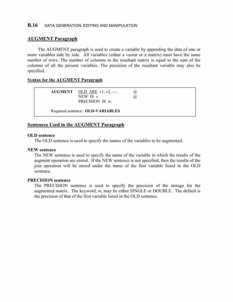
B.16 DATA GENERATION, EDITING AND MANIPULATION
AUGMENT Paragraph
The AUGMENT paragraph is used to create a variable by appending the data of one or more variables side by side. All variables (either a vector or a matrix) must have the same number of rows. The number of columns in the resultant matrix is equal to the sum of the columns of all the present variables. The precision of the resultant variable may also be specified.
Syntax for the AUGMENT Paragraph
Sentences Used in the AUGMENT Paragraph OLD sentence
The OLD sentence is used to specify the names of the variables to be augmented.
NEW sentence The NEW sentence is used to specify the name of the variable in which the results of the augment operation are stored. If the NEW sentence is not specified, then the results of the join operation will be stored under the name of the first variable listed in the OLD sentence.
PRECISION sentence The PRECISION sentence is used to specify the precision of the storage for the augmented matrix. The keyword, w, may be either SINGLE or DOUBLE. The default is the precision of that of the first variable listed in the OLD sentence.
AUGMENT OLD ARE v1, v2, ---. @ NEW IS v. @
PRECISION IS w. Required sentence: OLD-VARIABLES

APPENDIX C
GENERATING AND EDITING TIME SERIES DATA
Appendix B provided a review of several SCA capabilities to generate, edit and manipulate data in the SCA workspace. This appendix concentrates on those SCA capabilities to create or edit time series data in the SCA workspace. Features discussed in this appendix, and the section containing them, are:
Section Features C.1 Generation of variables for the modeling of a time series subject to trading day variation or an Easter holiday effect. C.2 Editing time series data by: recoding missing values; lagging or differencing data; temporal aggregation; and percent change in a series.
C.1 Generation of Some Useful Time Series
The SCA System provides capabilities for simulating ARIMA and transfer function models, and for generating some series useful in a time series analysis. Data simulation is discussed in Chapter 12 of The SCA Statistical System: Reference Manual for General Statistical Analysis. Simulated time series data are usually consonant with a specific ARIMA model (see Chapter 5) or transfer function model (see Chapter 8). We may also find generated data (that is, data completely specified in some manner) to be useful in data analyses. Such generated data include:
(a) Indicator variables. An indicator variable consists of binary (i.e., data that are either 0 or 1) and may be used to represent the time period(s) at which an intervention occurs (see Chapter 6 for more information on intervention analysis). The GENERATE paragraph (see Appendix B.1) is very convenient for creating indicator variables. (b) The number of Mondays, Tuesdays, . . ., Sundays in a month for a specified span of time. Variables with such information are useful when the effects of trading days are incorporated within an analysis of monthly time series. The generation and use of these variables are discussed in C.1.1. (c) Weights representing the proportion of an Easter effect duration period that occurs in the months prior to Easter for a specified period of time. The generation and use of these variables are discussed in C.1.2.

C.2 GENERATING AND EDITING TIME SERIES DATA
C.1.1 Generating data for the modeling of trading day variation
As noted in Chapter 8, transfer function models can be used to model time series data in the presence of certain calendar variation. One of these phenomena is trading day variation, another is the Easter holiday effect. The latter effect is discussed in Section C.1.2.
The DAYS paragraph can be used to generate the variables
.
i=1, 2, ..., 7, represents the number of times the day of the week (1=Monday, . . .,
7=Sunday) occurs in the month t. The DAYS paragraph can also provide a transformation of Wit. These variables are
,
where (i=1,2,...,6) reflects the number of times a day of the week occurs in a month
ber of Sundays in the month and is the total number of days in a month.
To illustrate the use of the DAYS paragraph, we will generate the number of Mondays, Tuesdays, ..., Sundays in each month during the period January 1949 through December 1960. The time span used here corresponds to that of the airline passengers data (Series G) in Box and Jenkins (1970). The data are used in Chapter 5 and are stored in the SCA workspace under the label SERIESG. To generate the data, and store the values in the variables MON, TUE, WED, THU, FRI, SAT and SUN, respectively, we may enter
-->DAYS MON,TUE,WED,THU,FRI,SAT,SUN. BEGIN 19491. END 1960,12.
The sentences BEGIN and END are required sentences providing the year and month of the beginning and ending of the time span. We will now use the PRINT paragraph to display the first 12 observations of SERIESG and the above seven variables. Some of the output is edited for presentation purposes.
-->PRINT SERIESG,MON,TUE,WED,THU,FRI,SAT,SUN. SPAN IS 1, 12. @ --> FORMAT IS 'F8.0, 7F4.0'.
VARIABLE SERIESG MON TUE WED THU FRI SAT SUN COLUMN--> 1 1 1 1 1 1 1 1 ROW 1 112 5 4 4 4 4 5 5 2 118 4 4 4 4 4 4 4 3 132 4 5 5 5 4 4 4 4 129 4 4 4 4 5 5 4 5 121 5 5 4 4 4 4 5
1 1t 2 2t 7 7tW W Wβ +β + ⋅⋅⋅+β
itW , thi
it it 7 tD W W , i 1,2,....,6= − =
7t 1t 2t 7tD W W W= + + ⋅⋅⋅+
itDrelative to the num 7tD

GENERATING AND EDITING TIME SERIES DATA C.3
6 135 4 4 5 5 4 4 4 7 148 4 4 4 4 5 5 5 8 148 5 5 5 4 4 4 4 9 136 4 4 4 5 5 4 4 10 119 5 4 4 4 4 5 5 11 104 4 5 5 4 4 4 4 12 118 4 4 4 5 5 5 4
As a second illustration of the DAYS paragraph, we will generate the transformed series
for the same time span as above. The transformed values are stored in D1 through D7, respectively. We will also specify an eighth variable, DATE. This optional variable will retain row labeling information (that is, year and month) corresponding to each year and month in the specified time span.
-->DAYS VARIABLES ARE D1 TO D7, DATE. BEGIN 1949,1. END 1960,12. @ --> TRANSFORM.
The logical sentence TRANSFORM is included to specify the generation of transformed
data. Note the complete form of the VARIABLES sentence is used (i.e., with sentence name and verb) to enable us to abbreviate the list of variable names D1, D2, D3, D4, D5, D6, D7, by “D1 to D7”. (For more information on abbreviations, please see Section 2.6.3 of The SCA Statistical System: Reference Manual for Fundamental Capabilities. As before, we will display only the first 12 observations of SERIESG, and the variables generated above. Again, some of the output is edited for presentation purposes.
-->PRINT VARIABLES ARE DATE, SERIESG, D1 TO D7. SPAN IS 1,12. @ --> FORMAT IS '2F8.0, 7F4.0'
VARIABLE DATE SERIESG D1 D2 D3 D4 D5 D6 D7 COLUMN--> 1 1 1 1 1 1 1 1 1 ROW 1 194901 112 0 -1 -1 -1 -1 0 31 2 194902 118 0 0 0 0 0 0 28 3 194903 132 0 1 1 1 0 0 31 4 194904 129 0 0 0 0 1 1 30 5 194905 121 0 0 -1 -1 -1 -1 31 6 194906 135 0 0 1 1 0 0 30 7 194907 148 -1 -1 -1 -1 0 0 31 8 194908 148 1 1 1 0 0 0 31 9 194909 136 0 0 0 1 1 0 30 10 194910 119 0 -1 -1 -1 -1 0 31 11 194911 104 0 1 1 0 0 0 30 12 194912 118 0 0 0 1 1 1 31
C.1.2 Generating data for the modeling of an Easter holiday effect
As noted in Chapter 8, a type of calendar effect known as a holiday effect occurs when consumer patterns or business activities vary due to a holiday. A transfer function model can be used to incorporate a variable of weights associated with a holiday effect within a time series model. The EASTER paragraph is used to generate a variable consisting of monthly weights related to the Easter holiday. The weights are based on the assumption that Easter has an effect on business activities in the period immediately preceding it. This effect is usually proportional to the amount of the Easter period that occurs in the months of March

C.4 GENERATING AND EDITING TIME SERIES DATA
and April each year. Proportions may differ between series reflecting the variability of when Easter occurs and the duration of the Easter period for a series. The term duration denotes the amount of time (i.e., the number of days) prior to Easter in which a series is likely to be affected. For example, the duration period for clothing sales may be much longer than that of floral sales.
The variable of weights generated by the EASTER paragraph has the value 0 for all months, with the exceptions of March and April. The values for these months are the fractions of the duration period occurring in the months. We need to specify the length, in days, of this duration period. The SCA System also displays the date for Easter in each of the years within our designated time span.
To illustrate the use of the EASTER paragraph, we will generate weights during the period January 1949 through December 1960. This time span is the same as the one used in Section C.1.2. We will assume the duration period to be 10 days. To generate a variable, say EASTERWT, we enter
-->EASTER EASTRWGT. BEGIN 1949,1. END 1960,12. DURATION IS 10.
THE DATES OF EASTER DURING THE REQUESTED TIME SPAN 1949 APRIL 17 1950 APRIL 9 1951 MARCH 25 1952 APRIL 13 1953 APRIL 5 1954 APRIL 18 1955 APRIL 10 1956 APRIL 1 1957 APRIL 21 1958 APRIL 6 1959 MARCH 29 1960 APRIL 17
The variable EASTERWT consists of the following weights
.0 .0 .0 1.0 .0 .0 .0 .0 .0 .0 .0 .0
.0 .0 .2 .8 .0 .0 .0 .0 .0 .0 .0 .0
.0 .0 1.0 .0 .0 .0 .0 .0 .0 .0 .0 .0
.0 .0 .0 1.0 .0 .0 .0 .0 .0 .0 .0 .0
.0 .0 .6 .4 .0 .0 .0 .0 .0 .0 .0 .0
.0 .0 .0 1.0 .0 .0 .0 .0 .0 .0 .0 .0
.0 .0 .1 .9 .0 .0 .0 .0 .0 .0 .0 .0
.0 .0 1.0 .0 .0 .0 .0 .0 .0 .0 .0 .0
.0 .0 .0 1.0 .0 .0 .0 .0 .0 .0 .0 .0
.0 .0 .5 .5 .0 .0 .0 .0 .0 .0 .0 .0
.0 .0 1.0 .0 .0 .0 .0 .0 .0 .0 .0 .0
.0 .0 .0 1.0 .0 .0 .0 .0 .0 .0 .0 .0
Non-zero values only occur in the months March and April. A weight has the value 1 when Easter occurs on or before April 1 or after April 11 (since we have defined the duration period prior to Easter to be 10 days). When Easter occurs between April 2 and April 10, inclusive, the weights for March and April are both non-zero (with the sum equal to 1.0), reflecting the proportion of the 10 day duration period occurring in each month.

GENERATING AND EDITING TIME SERIES DATA C.5
C.2 Editing Time Series Data
The SCA System provides many capabilities to edit or modify time series data. Missing data can be recoded and a new series can be created by lagging, differencing or aggregating the observations of an existing series. In addition, a series can be created by computing the percent change in the values of a series.
To illustrate some editing capabilities for time series data, we consider the first 40 observations of Series C of Box and Jenkins (1970). These data are assumed to be in the SCA workspace under the label SERIESC. In addition, we will omit a few values, replacing with them with missing values, in order to illustrate “patching” capabilities. The altered data are stored in the SCA workspace under the label SERIESCP. The data are listed below.
Initial forty observations of Series C of Box and Jenkins (1970) (SERIESC) and series with missing data (SERIESCP).
(Data are read across a line.)
SERIESC 26.6 27.0 27.1 27.1 27.1 27.1 26.9 26.8 26.7 26.4 SERIESCP 26.6 27.0 27.1 27.1 27.1 27.1 26.9 26.8 26.7 26.4 SERIESC 26.0 25.8 25.6 25.2 25.0 24.6 24.2 24.0 23.7 23.4 SERIESCP 26.0 25.8 25.6 **** **** 24.6 24.2 24.0 23.7 23.4 SERIESC 23.1 22.9 22.8 22.7 22.6 22.4 22.2 22.0 21.8 21.4 SERIESCP 23.1 22.9 22.8 22.7 22.6 22.4 22.2 22.0 21.8 21.4 SERIESC 20.9 20.3 19.7 19.4 19.3 19.2 19.1 19.0 18.9 18.9 SERIESCP 20.9 **** 19.7 19.4 19.3 19.2 19.1 19.0 18.9 18.9
C.2.1 Patching missing data
Special actions need to be taken when a time series contains missing observations. The SCA System provides capabilities for dealing with such series. Both the ACF and PACF paragraphs make necessary computational adjustments for missing observations when the logical sentence MISSING is included in the paragraph. A precise method to estimate the values of missing data in a time series is employed by the OESTIM paragraph. If the OESTIM paragraph is not available to us, we need to first recode missing data before estimating the parameters of a time series model. The recoded values should be “appropriate” so that they do not adversely affect an analysis and may reasonably represent the missing data. In this section, we explain some ad hoc methods that are generally useful.
To illustrate the replacement of missing data, we consider series SERIESCP. SERIESCP has the missing data code for the value of the 14th, 15th, and 32nd observations. We can recode a missing value directly using an analytic assignment statement (see Appendix B). Alternatively, we can employ some ad hoc methods through the PATCH paragraph. The PATCH paragraph provides us with some latitude in the recoding of time dependent data.

C.6 GENERATING AND EDITING TIME SERIES DATA
Since the values of the missing observations in SERIESCP are known to us, we are able to assess the validity of these methods in this case.
One simple scheme is to replace a missing value with the average of the values immediately adjacent to it. Adjacent averaging may be appropriate for nonstationary nonseasonal time series. To obtain adjacent averaging as a patching method for SERIESCP, we can enter
-->PATCH SERIESCP. METHOD IS ADJACENT(1). All missing values are replaced by the average of the values of the observations one time period from it. If two or more missing observations are next to each other, a missing value is replaced by the average of its two nearest, and equidistant, non-missing observations. Here we have
THE 14-TH OBSERVATION IS RECODED TO 25.2000 THE 15-TH OBSERVATION IS RECODED TO 24.9000 THE 32-TH OBSERVATION IS RECODED TO 20.3000
Here the 32nd observation is recoded to 20.3. Since observation 15 is missing, the 14th observation is recoded to the average of the 12th and 16th values. Similarly the 15th value is recoded to the average of observations 13 and 17. We can average the values of observations two time periods from each missing observation (or span of missing observations) by entering
-->PATCH SERIESCP. METHOD IS ADJACENT(2). We are informed that
THE 14-TH OBSERVATION IS RECODED TO 25.0000 THE 15-TH OBSERVATION IS RECODED TO 25.0000 THE 32-TH OBSERVATION IS RECODED TO 20.4000
The recoding for the 14th and 15th observations is as before. We can see that by
changing the argument in the METHOD sentence we can average “adjacent” information that is farther and farther away from a missing data point. This may be appropriate if we want to average adjacent, “December” or “1st quarter” data in the case of single missing observations for seasonal or periodic data. In such cases the value of the required argument of ADJACENT may be 12 or 4, respectively.
We can also replace missing data by the mean of all data, or a periodic mean (for seasonal data). This method of patching may be appropriate for seasonal and nonseasonal time series that have no trend over time. We can use the mean of all non-missing data as our replacement value by entering
-->PATCH SERIESCP. METHOD IS MEAN(1). As noted above, this is a reasonable way to recode missing data of a stationary time series. Since SERIESC is not stationary, and has a downward drift at its beginning, we observe this method of recoding is not inappropriate.

GENERATING AND EDITING TIME SERIES DATA C.7
THE 14-TH OBSERVATION IS RECODED TO 23.3622 THE 15-TH OBSERVATION IS RECODED TO 23.3622 THE 32-TH OBSERVATION IS RECODED TO 23.3622
If SERIESCP represented quarterly data, we may wish to use the mean of similar
quarters as a “patch”. We can specify this by entering
-->PATCH SERIESCP. METHOD IS MEAN(4).
THE 14-TH OBSERVATION IS RECODED TO 23.2889 THE 15-TH OBSERVATION IS RECODED TO 23.0889 THE 32-TH OBSERVATION IS RECODED TO 23.3889
We may only specify one method in the PATCH paragraph. If different methods are
appropriate (e.g., if the structure of the data changes over time), we can combine procedures by invoking the paragraph repeatedly but with different specifications in non-overlapping time spans. In addition, when we patch a series we can also create a binary indicator variable to highlight those time indices whose values were patched. If the PATCH paragraph is invoked repeatedly for the same series, using the same variable name for the binary indicator variable produces a indicator of all changes.
C.2.2 Lagging and differencing data
The time series capabilities of the SCA System (see Chapter 5) can incorporate differencing in the identification and estimation of time series models. However, it is sometimes useful to be able to lag or to difference data separately. The LAG and DIFFERENCE paragraphs provide these capabilities.
To illustrate the LAG paragraph, suppose we enter
-->LAG SERIESC. LAGS ARE 1, 2. NEW ARE LAGC1, LAGC2.
THE ORIGINAL SERIES IS SERIESC THE LAG 1 SERIES IS STORED IN VARIABLE LAGC1 , WHICH HAS 41 ENTRIES THE LAG 2 SERIES IS STORED IN VARIABLE LAGC2 , WHICH HAS 42 ENTRIES
We have generated two series, one stored in LAGC1 and the other in LAGC2. LAGC1
contains the first lag of SERIESC (that is, its first lag order). The i-th entry in LAGC1 is the (i-1)st entry of SERIESC. Hence,
LAGC15 = SERIESC4, LAGC120 = SERIESC19, LAGC141 = SERIESC40
The value of LAGC1(1) is necessarily undefined. In like manner, LAGC2 contains the second lag order of SERIESC. As a result, the contents of these variables are
SERIESC LAGC1 LAGC2 1 26.600 *** *** 2 27.000 26.600 ***

C.8 GENERATING AND EDITING TIME SERIES DATA
3 27.100 27.000 26.600 4 27.100 27.100 27.000 5 27.100 27.100 27.100 6 27.100 27.100 27.100 . . . . . . . . . . . . 38 19.000 19.100 19.200 39 18.900 19.000 19.100 40 18.900 18.900 19.000 41 18.900 18.900 42 18.900
A first lag order is assumed if the LAG sentence is not specified. Lagged values are
stored as indicated above so that information is properly aligned if we wish to investigate relationships between the currently observed value of one variable and a previous (lagged) observation of another variable.
We difference data in a manner similar to lagging. For example, the first-order differenced series of SERIESC is
t t t(1 B)SERIESC SERIESC B(SERIESC ), or− = −
tained. We obtain this new
series by entering
-->DIFFERENCE SERIESC. NEW IS DIFFC1. 1 DIFFERENCE ORDERS ARE (1-B ) SERIES SERIESC IS DIFFERENCED, THE RESULT IS STORED IN VARIABLE DIFFC1 SERIES DIFFC1 HAS 40 ENTRIES
Similarly we can calculate (1-B)(
t t 1 SERIESC SERIESC −= −
The subscript t has been included to indicate how values are ob
41 B− )SERIESC. This result is related to what we have calculated, since
t 4 .
We can obtain this differenced series by entering
-->DIFFERENCE SERIESC. NEW IS DIFFC14. DFORDERS ARE 1, 4.
1 4 DIFFERENCE ORDERS ARE (1-B ) (1-B ) SERIES SERIESC IS DIFFERENCED, THE RESULT IS STORED IN VARIABLE DIFFC12 SERIES DIFFC12 HAS 40 ENTRIES
A partial listing of the values in these variables is given below
SERIESC DIFFC1 DIFFC14 1 26.600 *** *** 2 27.000 .400 *** 3 27.100 .100 ***
4 4t t t(1 B)(1 B )SERIESC (1 B )DIFFC1 DIFFC1 DIFFC1 −− − = − = −

GENERATING AND EDITING TIME SERIES DATA C.9
4 27.100 .000 *** 5 27.100 .000 *** 6 27.100 .000 -.400 7 26.900 -.200 -.300 8 26.800 -.100 -.100 9 26.700 -.100 -.100 10 26.400 -.300 -.300 . . . . . . . .
C.2.3 Temporal aggregation
Occasionally a time series is recorded at one time interval (for example, monthly or quarterly), but an analysis utilizes a longer time interval (for example, quarterly or yearly). The data recorded at the more frequent time interval must then be transformed by means of temporal aggregation for the purpose of analysis. For more information on temporal aggregation, please see Chapter 16 of Wei (1990).
The AGGREGATE paragraph is used to generate a new time series through the temporal aggregation of a specified time series. The generated series will be calculated from non-overlapping time intervals of a length that we specify. Aggregation is based on either the aggregate sum or the aggregate mean of the data values in each period. When there are fewer data points than the specified aggregation period in either the first or the last group, the mean of the data available within the group is computed and used accordingly. If we choose the aggregate sum as the method for aggregation, the SCA System will first compute an aggregate mean for each group, and then multiply this mean by the designated interval length. This method of aggregation may not be appropriate for a series that is highly seasonal or has a trend, and that has an incomplete group at its beginning or end.
To illustrate the AGGREGATE paragraph, we will use the airline data (SERIESG) used previously in this appendix and in Chapter 5. The monthly totals of airline passengers are aggregated to quarterly totals. We can aggregate the series to a new series, QSERIESG, by entering
-->AGGREGATE SERIESG. NEW IS QSERIESG. METHOD IS SUM (3).
The method SUM(3) indicates that the sum of each non-overlapping set of 3 observations is used for aggregation. Since we have 144 observations in SERIESG, we will have 48 observations in QSERIESG with no incomplete groups during aggregation. The values of the variable QSERIESG are shown below.
362 385 432 341 382 409 498 387 473 513 582 474 544 582 681 557 628 707 773 592 627 725 854 661 742 854 1023 789 878 1005 1173 883 972 1125 1336 988 1020 1146 1400 1006 1108 1288 1570 1174 1227 1468 1736 1283

C.10 GENERATING AND EDITING TIME SERIES DATA
C.2.4 Percentage change in a series
Often it is useful to analyze the percent change of the values of a time series rather than the originally recorded observations of the series. The PERCENT paragraph is used to compute the percent change of values of a time series and store the results in a new variable.
To compute percentages for a series, we need to specify a period and a method for computation. The period allows us to base calculations on adjacent points if the length of the period is 1. We can obtain a seasonal percent change in monthly data by using 12 as the length of period.
Two methods of computation are available. A simple percent change uses the previous observation as a base; that is,
(Y(t) Y(t i))*100T(t i)− −
−
A symmetric percent change computation uses an average of observed values as a base;
that is, (Y(t) Y(t i))*100
Y(t) Y(t i)2
− −+ −
,
where i is the specified period length. The default method of computation is a simple percent change of adjacent points (i.e., SIMPLE(1)).
To illustrate the use of different periods in computations, we will again consider the airline data, SERIESG. If we wish to use the default method of computation (i.e., the simple percent change of adjacent points), we can simply enter
-->PERCENT SERIESG. NEW IS SERIESG1.
The percent changes are stored in the variable SERIESG1. Since the airline data is seasonal, we can compute a simple seasonal percent change by entering
-->PERCENT SERIESG. NEW IS SERIESG2. METHOD IS SIMPLE (12).
The percent changes are stored in the variable SERIESG2. We will now use the PRINT paragraph to display the first 24 observations of each series (output edited for presentation purposes).
-->PRINT SERIESG, SERIESG1, SERIESG2. SPAN IS 1, 24.
VARIABLE SERIESG SERIES1 SERIES2 COLUMN--> 1 1 1 ROW 1 112.000 *** *** 2 118.000 5.357 *** 3 132.000 11.864 ***

GENERATING AND EDITING TIME SERIES DATA C.11
4 129.000 -2.273 *** 5 121.000 -6.202 *** 6 135.000 11.570 *** 7 148.000 9.630 *** 8 148.000 .000 *** 9 136.000 -8.108 *** 10 119.000 -12.500 *** 11 104.000 -12.605 *** 12 118.000 13.462 *** 13 115.000 -2.542 2.679 14 126.000 9.565 6.780 15 141.000 11.905 6.818 16 135.000 -4.255 4.651 17 125.000 -7.407 3.306 18 149.000 19.200 10.370 19 170.000 14.094 14.865 20 170.000 .000 14.865 21 158.000 -7.059 16.176 22 133.000 -15.823 11.765 23 114.000 -14.286 9.615 24 140.000 22.807 18.644
We see that the internal missing value code is used whenever a percent change cannot
be computed.

C.12 GENERATING AND EDITING TIME SERIES DATA
SUMMARY OF THE SCA PARAGRAPH IN APPENDIX C
This section provides a summary of the SCA paragraph employed in this appendix. An
SCA paragraph begins with a paragraph name and is followed by modifying sentences. Sentences that may be used as modifiers for a paragraph are shown below and the types of arguments used in each sentence are also specified. Sentences not designated required may be omitted as default conditions (or values) exist. The most frequently used required sentence is given as the first sentence of the paragraph. The portion of this sentence that may be omitted is underlined. This portion may be omitted only if this sentence appears as the first sentence in a paragraph. Otherwise, all portions of the sentence must be used. The last character of each line except the last line must be the continuation character, ‘@’.
The paragraphs explained in this summary are DAYS, EASTER, PATCH, LAG, DIFFERENCE, AGGREGATE, and PERCENT.
Legend (see Chapter 2 for further explanation) v : variable name i : integer r : real value w( ) : keyword (with argument) DAYS Paragraph
⋅
The DAYS paragraph is used to generate seven variables containing the number of Mondays, Tuesdays, ..., Sundays in a month for a given period of time. The number of rows generated corresponds to the number of months in the specified time span. An optional eighth variable may also be specified to retain row labeling information (year and month) corresponding to each year and month in the specified time span. The generated series may then be transformed according to
,
where is the number of occurrences of the i-th day (1=Monday, . . ., 7=Sunday) in the t-th month.
it it 7 tD W W , i 1,2,3,...,6= − =
7t 1t 2t 7tD W W W= + + ⋅⋅⋅+
itW

GENERATING AND EDITING TIME SERIES DATA C.13
Syntax for the DAYS Paragraph
Sentences Used in the DAYS Paragraph VARIABLES sentence
The VARIABLES sentence is used to specify the names of seven variables in which the number of days of a month will be stored. The first seven variables contain information regarding the number of days in a month in the following order: Mondays (v1), Tuesdays (v2), . . ., Sundays (v7). An eighth variable may also be specified to store labeling information. The labeling information consists of the year and month corresponding to each row. The number of rows generated is dependent on the time span specified in the BEGIN and END sentences. One row will be generated for each month between the specified beginning and ending month, inclusive.
BEGIN sentence The BEGIN sentence is used to specify the beginning year, i1 (1901-2100), and month, i2 (1 for January, . . ., 12 for December), from which monthly information on days will be generated.
END sentence The END sentence is used to specify the ending year, i1 (1901 - 2100), and month, i2 (1 for January, ..., 12 for December), through which monthly information on days will be generated. The year and month specified must be later than that specified in the BEGIN sentence.
TRANSFORM sentence The TRANSFORM sentence specifies the generation of a set of transformed data according to the transformation defined above. The default is NO TRANSFORM. Transformed data replace the data stored in the variables specified in the VARIABLES sentence as follows: v1( ), v2( , . . ., v7( .
DAYS VARIABLES ARE v1, v2, ---, v8. @ BEGIN IN i1, i2. @ END IN i1, i2. @ TRANSFORM./NO TRANSFORM.
Required sentences: VARIABLES, BEGIN, END
1tD 2tD ) 7tD )

C.14 GENERATING AND EDITING TIME SERIES DATA
EASTER Paragraph
The EASTER paragraph is used to generate a variable consisting of monthly weights related to the Easter holiday. The weights (values between 0 and 1) indicate the proportion of the Easter effect occurring in each month during the specified time period. Thus, the weight is usually 0 for all months with the exceptions of March and April. An optional second variable may be created to retain row labeling information (year and month) corresponding to each year and month in the specified time span.
Syntax for the Easter Paragraph
Sentences VARIABL
The VAweightsis specifvariable
BEGIN senThe BE(1 for Jwill be g
END sentenThe ENJanuarybe genesentence
DURATIOThe DUEaster h
EASTER VARIABLES ARE v1, v2. @ BEGIN IN i1, i2. @ END IN i1, i2. @ DURATION IS i.
Required sentences: VARIABLES, BEGIN, END and DURATION
Used in the EASTER Paragraph
ES sentence RIABLES sentence is used to specify the label of the variable in which the
(between 0 and 1) related to the Easter holiday will be stored. If a second variable ied, it will be used to store year and month labeling information. The length of the generated depends on the time span specified in the BEGIN and END sentences.
tence GIN sentence is used to specify the beginning year, i1 (1901-2100), and month, i2 anuary, ..., 12 for December), from which monthly information on Easter effect enerated.
ce D sentence is used to specify the ending year, i1 (1901-2100), and month, i2 (1 for , . . ., 12 for December), through which monthly information on Easter effect will rated. The year and month specified must be later than that specified in the BEGIN .
N sentence RATION sentence is used to specify the duration (i.e., the number of days) of the oliday effect prior to each Easter holiday. This is a required sentence.

GENERATING AND EDITING TIME SERIES DATA C.15
PATCH Paragraph
The PATCH paragraph is used to recode missing data of a time series by replacing missing values with one of the following:
(1) the average of the two observations that are i indices adjacent to it,
(2) the mean of all observations or those non-missing observations i indices apart from the missing value, or
(3) a specified value. In addition, a binary indicator variable can be created to provide a reference variable highlighting those time indices whose values were patched. Syntax of the PATCH Paragraph
Sentences Used in the PATCH Paragraph OLD sentence
The OLD sentence is used to specify the name of the variable containing missing data.
NEW sentence The NEW sentence is used to specify the name of the variable to store the patched series. The default is the name specified in the OLD series.
METHOD sentence The METHOD sentence is used to specify the method used to recode missing data in the OLD variable. Keywords and associated arguments that may be used to specify the method are:
(1) ADJACENT(i): all missing data are recoded to the average of the values of the OLD series with indices (t-i) and (t+i), where t is the index of the missing value.
(2) MEAN(i): all missing data are recoded to the periodic average of the non-missing values of the OLD series. The argument i is used to specify the periodicity of the series. If i=1 then the overall average of all non- missing data will be used to recode the missing observations.
PATCH OLD IS v. @ NEW IS v. @
METHOD IS w(i). @ SPAN IS i1, i2. @
INDICATOR IS v. Required sentence: OLD

C.16 GENERATING AND EDITING TIME SERIES DATA
(3) VALUE(r): all missing data are recoded to the value r.
The methods are all mutually exclusive within the execution of a single paragraph. The default is ADJACENT(1).
SPAN sentence The SPAN sentence is used to specify the span of time indices, i1 to i2, in which a patch of missing data will be made. The default span is the whole series.
INDICATOR sentence The INDICATOR sentence is used to specify a name (label) for an indicator variable associated with the patching. The indicator variable contains 1 for missing data that are replaced, and 0 otherwise. The length of the indicator variable is always the same as the old series regardless of the time periods specified in the SPAN sentence. This convention allows use of the same indicator variable for multiple patches of a series using different methods.
LAG Paragraph
The LAG paragraph is used to apply the lag (backshift) operator, B, to a variable to create a new lagged variable. For the variable X, the lag operation Y = B(X) is defined as
1 provided it exists (otherwise a missing value code is provided). This definition is for a lag one backshift. Various other lag orders may be specified (e.g., lag k, where
k for various values of k), hence creating more than one new series.
Lagged values are stored in the following manner. If the variable YDATA stores the k-th order lagged values of the variable XDATA, then
YDATA(t) = the missing value code, j = 1,2,. . .,k = XDATA(t-k), t = k+1,. . .,k+n where n is the index of the last observation (value) of XDATA. As a result, YDATA has (n+k) observations, the first k of which containing the missing value code, while XDATA has n observations. Syntax for the LAG Paragraph
t tY X −=
t tY X −=
LAG OLD IS v. @ NEW ARE v1, v2, --- . @ LAGS ARE i1, i2, --- . Required sentence: OLD

GENERATING AND EDITING TIME SERIES DATA C.17
Sentences Used in the LAG Paragraph OLD sentence
The OLD sentence is used to specify the name of the series to lag.
NEW sentence The NEW sentence is used to specify names of the new series. Results will be stored in the OLD series if the NEW sentence is omitted.
LAGS sentence The LAGS sentence is used to specify the lags to be made on the old series. For example, if there are 3 specified lags, three new series will be generated. The default is 1, creating
1 .
DIFFERENCE Paragraph
t tY X −=
The DIFFERENCE paragraph is used to apply the operator to a variable or a set of variables to create one or more variables. For a variable X, the operation is defined as j provided t > j (otherwise a missi s
FORDER) in the backshifay be specified. If
r w variab e the m ed as the f rst (i1+i2+××of the resulting variable. The missing values may be deleted and the resulting variable compressed to a series containing n(-i1+i2+×××+im) values, where n is the number of observations of the original series, if the COMPRESS sentence is specified.
Syntax for the DIFFERENCE Paragraph
j(1 B )−
ng value is
differencing orders, i1, i2, . . .ill be applied
i
jY (1 B )X= − specified). Thi
t operator B. More , im, are
to all designated×+im) values
t t tY X X −= −definition is given for one differencing order (Dthan one differencing order mspecified, then the operato
les. In such a casi1 i2 im(1 B )(1 B )....(1 B )− − −
issing value code is stor
DIFFERENCE OLD ARE v1, v2, --- . @ NEW ARE v1, v2, --- . @ DFORDERS ARE i1, i2, --- . @ COMPRESS. /NO COMPRESS. Required sentence: OLD

C.18 GENERATING AND EDITING TIME SERIES DATA
Sentences Used in the DIFFERENCE Paragraph OLD sentence
The OLD sentence is used to specify the name(s) of the series to be differenced.
NEW sentence The NEW sentence is used to specify the variable name(s) where the differenced series are stored. The default is that the data will be stored in the names specified in the OLD sentence.
DFORDERS sentence The DFORDERS sentence is used to specify the orders in the product of differencing operators to be made on the OLD series. Default is 1, the single operator (1-B). If i1, i2, . . . are specified, the operator . . . is applied to the old series.
COMPRESS sentence The COMPRESS sentence is used to indicate whether the missing values caused by differencing will be deleted. When COMPRESS is specified, the resulting NEW variable will have fewer observations than its corresponding OLD variable. The first value of the NEW variable will be the first value for which the differencing operator is valid. Default is NO COMPRESS, i.e., the missing value code will be assigned to all undefined values and the NEW variable will have as many observations as its corresponding OLD variable.
AGGREGATE Paragraph
i1 i2(1 B )(1 B )....− −
The AGGREGATE paragraph is used to generate a new time series through the temporal aggregation of a specified time series. More than one series can be aggregated at a time.
Syntax of the AGGREGATE Paragraph
AGGREGATE OLD IS v1, v2, ---. @ NEW IS v1, v2, ---. @ BEGINNING IS i. @
METHOD IS w(i). @ SPAN IS i1, i2. @
COMPRESS./NO COMPRESS. Required sentences: OLD, METHOD

GENERATING AND EDITING TIME SERIES DATA C.19
Sentences Used in the AGGREGATE Paragraph OLD sentence
The OLD sentence is used to specify the name(s) of time series variable(s) from which aggregated time series will be derived.
NEW sentence The NEW sentence is used to specify the name(s) of variable(s) to store the aggregated time series. The default is to use the names specified in the OLD sentence.
BEGINNING sentence The BEGINNING sentence is used to specify the index for which aggregation will begin. The default is 1, i.e., the first period.
METHOD sentence The METHOD sentence is used to specify the manner of, and period for, temporal aggregation. The associated keywords are SUM in which the aggregate sum of each nonoverlapping interval is recorded and MEAN in which the aggregate average of each nonoverlapping interval is recorded. The integer argument for each keyword is used to specify the time period used in the temporal aggregation. Values 1 to i of the each variable specified in the OLD sentence are aggregated to the first value of the stored in the variable(s) specified in the NEW sentence; values i+1 to 2i are aggregated to the second value; and so on. Indexing values are shifted appropriately if the value specified in the BEGINNING sentence is not 1.
SPAN sentence The SPAN sentence is used to specify the span of time indices, from i1 to i2, in which aggregate time series will be generated. The default span is the whole series.
COMPRESS sentence The COMPRESS sentence is used to specify that the generated series will be stored in condensed form, i.e., aggregated observations are not repeated so that the total number of observations are less than that of the original series. The default is COMPRESS.

C.20 GENERATING AND EDITING TIME SERIES DATA
PERCENT Paragraph
The PERCENT paragraph is used to generate a new time series using the percent change in the observations of a specified time series. More than one series can be generated simultaneously.
Syntax for the PERCENT paragraph
Sentences OLD sente
The OLpercent
NEW senteThe NEchange
METHOD The MEcomputaSYMMEmethod
(Y
The (Y
The SPAN sente
The SPAcomputa
PERCENT OLD ARE v1, v2, --- . @ NEW ARE v1, v2, --- . @ METHOD IS w(i). @ SPAN IS i1, i2.
Required sentence: OLD
Used in the PERCENT Paragraph
nce D sentence is used to specify the name(s) of time series variable(s) for which the change will be derived.
nce W sentence is used to specify the name(s) of variable(s) to store the percent
time series. The default is to use the names specified in the OLD.
sentence THOD sentence is used to specify the method and the period used in the tion of the percent change. The keyword w can be either SIMPLE or TRIC. The associated period length (i) must also be specified. The SIMPLE
computes the percent change using the formula
(t) Y(t i))*100Y(t i)− −
−.
SYMMETRIC method uses the formula
(t) Y(t i))*100Y(t) Y(t i)
2
− −+ −
,
default is SIMPLE(1).
nce N sentence is used to specify the span of time indices, from i1 to i2, in which the tion of percent change will be made. The default span is the whole series.

GENERATING AND EDITING TIME SERIES DATA C.21
REFERENCES
Box, G.E.P. and Jenkins, G.M. (1970). Time Series Analysis: Forecasting and Control. San Francisco: Holden Day. (Revised edition published in 1976).
Wei, W.W.S. (1990). Time Series Analysis: Univariate and Multivariate Methods. New York: Addison-Wesley.


APPENDIX D
SCA MACRO PROCEDURES
The SCA System provides us with the capability to create and maintain computations,
analyses or procedures specific to our needs. For example, we may find it useful to perform a special sequence of SCA operations with different data during an SCA session. It would simplify our work if such sequences can be written only once and then could be freely referred to subsequently. Many programming languages provide subprograms to help in this situation. SCA offers macro procedures to obtain such flexibility.
The use of an SCA macro procedure enables us to store any set of SCA statements on a file which may be referenced at any point of an SCA session. This enables us to extend the capabilities of the SCA System.
D.1 SCA Macro Files and Macro Procedures
SCA macro procedures are maintained in files. These files are referred to as SCA macro files. Procedures contained on a macro file may be created by any text editor.
An SCA macro procedure consists of a sequence of SCA statements, including both analytic and English-like statements. A macro procedure is handled as a “subprogram” within an SCA session.
To illustrate SCA macro files and SCA macro procedures, Tables D.1 and D.2 list the contents of two SCA macro files. These files will be used throughout this Appendix to illustrate SCA macro procedures. The records of Table D.1 and Table D.2 comprise the files APPENDX.DATA and MACRO.DATA, respectively. The names of the files are for illustration only and may be changed to names appropriate to a local computer.

D.2 SCA MACRO PROCEDURES
Table D.1 Contents of the file APPENDX.DATA
==ALL MACRO CALL APPENDXA CALL APPENDXB RETURN ==APPENDXA --A MACRO PROCEDURE ILLUSTRATING THE MATRIX EXAMPLES --OF APPENDIX A INPUT ADATA, BDATA, EDATA. NCOL ARE 2, 3, 3. 1 1 1 3 0 3 -1 0 3 1 2 1 0 -1 2 -1 0 1 0 1 -1 0 -1 3 END OF DATA C1DATA = BDATA # ADATA C2DATA = T(ADATA) # BDATA DETB = DET(BDATA) PRINT C1DATA, C2DATA, DETB BINVERSE = INV(BDATA) ADJOINTB = DETB*BINVERSE PRINT BINVERSE, ADJOINTB EIGEN EDATA RETURN ==APPENDXB --A MACRO PROCEDURE OF THE SCA STATEMENTS IN SECTION B.1.1 --AND B.1.2 OF APPENDXB GENERATE VECTOR1. NROW ARE 10. VALUES ARE 0 FOR 5, 1 FOR 5. GENERATE VECTOR2. NROW ARE 10. VALUES ARE 0 FOR 5, 1 FOR 2, 0 FOR 3. GENERATE VECTOR3. NROW ARE 10. PATTERN IS STEP(1.0, 0.5). GENERATE VECTOR4. NROW ARE 10. PATTERN IS RATE(1.0, 2.0). PRINT VECTOR1, VECTOR2, VECTOR3, VECTOR4 RETURN //

SCA MACRO PROCEDURES D.3
Table D.2 Contents of the file MACRO.DATA
==SCORES C @ C AVERAGE ENGLISH SCORES @ C INPUT VARIABLE IS ENGLISH. 82 14 25 67 48 76 23 46 96 69 66 62 70 88 61 72 END OF DATA C @ C AVERAGE PHYSICS SCORES @ C INPUT VARIABLE IS PHYSICS. 86 72 34 92 68 74 69 35 75 24 33 END OF DATA RETURN ==EXPLORE C @ C AS A MEANS TO GET A FEEL FOR A DATA SET, @ C A CONFIDENCE INTERVAL AND PLOT OF DATA @ C OVER TIME WILL BE INVOKED. @ C DATA ARE ASSUMED TO BE STORED IN THE SCA WORKSPACE @ C IN A VARIABLE NAMED X. @ C CINTERVAL X TSPLOT X RETURN ==LINREG PARAMETER SYMBOLIC-VARIABLES ARE NINDEP, FILE(12). C @ C READ IN DATA @ C INPUT VARIABLES ARE Y,X. FILE IS &FILE. @ NCOLS ARE 1, &NINDEP. C @ C COMPUTE REGRESSION COEFFICIENTS, PREDICTED VALUES, RESIDUALS, ETC. @ C BETA = INV(T(X)#X)#T(X)#Y -- COMPUTE REGRESSION COEFFICIENTS YHAT = X#BETA -- COMPUTE PREDICTED VALUES RESI = Y-YHAT -- COMPUTE RESIDUALS N = NROW(X) P = NCOL(X) NP = N-P P1 = P-1 MEAN = SUM(Y)/N SST = SUM((Y-MEAN)**2) SSE = SUM(RESI**2) SSB = SST-SSE MSE = SSE/NP MSB = SSB/P1 F = MSB/MSE C @ C PRINT REGRESSION COEFFICIENTS @ C DO 100 I=1,P I1=I-1 IF(I1 LE 9) THEN NEXT ELSE GO FORWARD 80 DISPLAY TEXT IS T5,'BETA',I1('F1.0'),' = ',BETA('F12.4',I). GO FORWARD 100 80 DISPLAY TEXT IS T5,'BETA',I1('F2.0'), ' = ',BETA('F12.4'',I). 100 CONTINUE

D.4 SCA MACRO PROCEDURES
Table 2 Contents of the file MACRO.DATA (continued)
C @ C PRINT THE ANALYSIS OF VARIANCE TABLE @ C DISPLAY TEXT IS ///T5,'ANALYSIS OF VARIANCE TABLE'// @ T5,' SOURCE D.F. SUM OF SQUARES MEAN SQUARES F'/. DISPLAY TEXT IS T5,'REGRESSION',P1('F6.0',1),SSB('C17.4',1), @ MSB('C15.4',1),F('C10.2',1). DISPLAY TEXT IS T5,' ERROR ',NP('F6.0',1),SSE('C17.4',1), @ MSE('C15.4',1). DISPLAY TEXT IS T5,' TOTAL ',N ('F6.0',1),SST('C17.4',1) RETURN //
D.2 Structure of an SCA Macro File
Both files APPENDX.DATA and MACRO.DATA have similar structure. A set of SCA commands, or data, are preceded by a record with double equal signs (i.e., ‘= =’) in columns 1 and 2; and are ended with the statement RETURN. The final entry of each file is ‘//’.
The alphanumeric characters following ‘= =’ provide the name of the macro procedure. For example, the file APPENDX.DATA consists of the macro procedures named ALLMACRO, APPENDXA and APPENDXB; while MACRO.DATA contains the macro procedures SCORES, EXPLORE and LINREG. The name of a macro procedure may contain from one to eight alphanumeric characters, with a letter as the mandatory first character. If more than eight characters are used as a macro procedure name, only the first eight characters are interpreted.
Any line with the letter C in the first column and a space in the second column (i.e., ‘C’) is interpreted as a line of comments. Any line whose first non-blank entries are a double dash (‘--‘) is also interpreted as a line of comments. Lines beginning with ‘--‘ are not printed, but those beginning with ‘C’ will be printed as they are interpreted during an SCA session.
D.3 Invoking a Macro Procedure
If we enter the command
-->CALL APPENDXB. FILE IS 'APPENDX.DATA'. then the following set of SCA commands will be interpreted and executed
GENERATE VECTOR1. NROW ARE 10. VALUES ARE 0 FOR 5, 1 FOR 5. GENERATE VECTOR2. NROW ARE 10. VALUES ARE 0 FOR 5, 1 FOR 2, 0 FOR 3. GENERATE VECTOR3. NROW ARE 10. PATTERN IS STEP(1.0, 0.5). GENERATE VECTOR4. NROW ARE 10. PATTERN IS RATE(1.0, 2.0). PRINT VECTOR1, VECTOR2, VECTOR3, VECTOR4

SCA MACRO PROCEDURES D.5
These commands will duplicate selected capabilities illustrated in Appendix B. Similarly, if we enter
-->CALL APPENDXA. FILE IS 'APPENDX.DATA' then selected capabilities illustrated in Appendix A will be computed and results displayed.
The macro procedure SCORES of MACRO.DATA will transmit two variables, stored as ENGLISH and PHYSICS, to the SCA workspace. The procedure named EXPLORE can be used for computing a confidence interval and a time series plot of a variable. For example, suppose we have three variables, SERIESA, SERIESB, and SERIESC, in the SCA workspace. We can repeatedly perform these operations by entering the sequence of commands
-->X = SERIESA -->CALL EXPLORE. FILE IS 'MACRO.DATA'. -->X = SERIESB -->CALL EXPLORE -->X = SERIESC -->CALL EXPLORE
We may note that after the first CALL to the EXPLORE macro procedure the FILE
sentence is omitted. Unless it is instructed otherwise, the SCA System assumes a macro procedure being called resides in the last referenced macro file. This default is implicit within the macro procedure ALLMACRO of the APPENDX.DATA file. If we enter
CALL ALLMACRO. FILE IS 'APPENDX.DATA'. we see that calls to the remaining macro procedures of the file are invoked, hence all macro procedures of the file are executed. Care must be taken if one or more macro procedures is nested within another. That is, an error can occur if one macro procedure calls another. Appropriate allocation and de-allocation of files is required. Please refer to Section 1 of Appendix E for further information.
D.4 Symbolic Variables in a Macro Procedure
Symbolic Variables
The term “symbolic variables” refers to any name used in a macro procedure to label a variable or entry that can be given a new value or connotation when a macro procedure is invoked. Symbolic variables add flexibility to macro procedures by labeling actual arguments that may change when a procedure is executed. For example, it is desirable to be able to pass a different series name (or variable name) to the EXPLORE procedure in MACRO.DATA rather than requiring a variable to have X as its name for all uses of the procedure. To facilitate this convenience, the label X may be replaced by an expression, such as &SERIES,

D.6 SCA MACRO PROCEDURES
in the procedure. In this manner, SERIES is recognized by the system as a symbolic variable as explained below.
Within the body of a macro procedure a symbolic variable is denoted by preceding a string of alphanumeric characters by an ampersand (&). The first character of the string must be a letter and the last character may be a compound symbol (#). The compound symbol is used as a deliminator if the symbol variable is immediately followed by a number or letter. The name of the symbolic variable is the character string excluding the compound symbol. The compound symbol can be omitted if the symbolic variable name is immediately followed by a special character such as blank, ‘.’ or ‘, ‘. If the alphanumeric string denoting the symbolic variable has more than eight characters, only the first eight are interpreted. The special character ‘&’ is used to distinguish symbolic variables from other variables used in a macro procedure. The actual values used for the symbolic variables are supplied when the macro procedure is invoked (by the CALL paragraph, see syntax at the end of this Appendix), or may be those values supplied as default values within the procedure itself. In the SCA interactive mode, if a symbolic variable does not have a default value and is not supplied in the CALL paragraph, the SCA System will issue a prompt for a value. The response to the prompt must be enclosed in a pair of parentheses. A fatal error will occur if such a situation happens in the batch environment.
Symbolic Substitution
The SCA System scans each line in a macro procedure and replaces symbolic variables with their actual values in an action called symbolic substitution. An actual argument for a symbolic variable is always stored in its exact character form. For example, if a symbolic variable has a value 2.3, it is stored as a string of three characters ‘2.3’, rather than a real number. Hence symbolic substitution will not lose any precision. The rule governing symbolic substitution is simple: the SCA System scans a line in the macro procedure from right to the left and substitutes the first symbolic variable encountered by its associated value (in character form). This scanning is repeated until all symbolic variables are substituted and resolved. This rule allows the user to concatenate symbolic variables to modify existing variable names, or to use multiple ampersands. For example, if &A has the symbolic argument JOHN, and &JOHN has the symbolic argument BOY, then &&A will have the value BOY after the completion of symbolic substitution. The symbolic variables may appear anywhere in a statement in an SCA macro procedure although they usually appear in analytic expressions or argument lists of assignment sentences.
D.5 A Regression Macro Procedure
To illustrate both the use of symbolic variables and the ability to write our own procedures, we consider the macro procedure LINREG of the MACRO.DATA file (see Table D.2). LINREG performs a regression analysis using analytic expressions (see Appendix A). This procedure may be useful in teaching regression analysis, but a more computationally efficient means is available through the SCA REGRESS paragraph (see Chapter 4).

SCA MACRO PROCEDURES D.7
The macro procedure transmits data for the dependent and independent variables from a file. The symbolic argument FILE is used to designate the logical unit number for the file containing the data. If a unit number is not specified in the CALL paragraph, the default unit 12 is used. This default value is specified within the LINREG macro in the PARAMETERS paragraph (its complete syntax is provided at the end of this Appendix).
Within the file FILE the first column of data is transmitted to the dependent variable labeled Y and the remaining p columns contain the independent variables, stored in the matrix X. The value p is represented in the macro by the symbolic argument NINDEP. This argument has no default value, hence we must specify it in our CALL of LINREG.
The data listed in Table D.3 is assumed to be on a file that has been associated with the logical unit 12. This assignment may have been accomplished before we invoked the SCA System or through the ASSIGN paragraph (see Appendix E).
Table D.3 Data used in the LINREG example
101 1 1 1 1 106 1 1 1 1 87 1 1 1 1 131 1 1 1 1 265 1 1 2 2 272 1 1 2 2 279 1 1 2 2 302 1 1 2 2 106 1 2 1 2 89 1 2 1 2 128 1 2 1 2 103 1 2 1 2 291 1 2 2 4 306 1 2 2 4 334 1 2 2 4 272 1 2 2 4
To invoke the LINREG procedure on this data set we can enter
-->CALL LINREG. FILE IS 'MACRO.DATA'. @ SYMBOLIC IS NINDEP(4).
We will obtain output similar to that given below.

D.8 SCA MACRO PROCEDURES
REGRESSION COEFFICIENTS: BETA0 = -46.2500 BETA1 = -20.7500 BETA2 = 152.2500 BETA3 = 21.0000 ANALYSIS OF VARIANCE TABLE SOURCE D.F. SUM OF SQUARES MEAN SQUARES F REGRESSION 3 135,959.5000 45,319.8330 117.73 ERROR 12 4,619.5000 384.9583 TOTAL 16 140,579.0000
D.6 Global and Local Variables
A variable with ‘@’ as the first character of its name is treated as a local variable within a macro procedure. Others are regarded as global variables. The difference between a local and global variable is that local variables are deleted from the workspace upon completion of a macro procedure, unless otherwise specified. A local variable may be retained in the workspace by using the RETAIN sentence in the RETURN paragraph (see the Syntax section at the end of this Appendix). Global variables may be used anywhere in a session, including in subsequent macro procedures.

SCA MACRO PROCEDURES D.9
SUMMARY OF THE SCA PARAGRAPHS IN APPENDIX D
This section provides a summary of those SCA paragraphs employed in this chapter.
Each SCA paragraph begins with a paragraph name and is followed by modifying sentences. Sentences that may be used as modifiers for a paragraph are shown below and the types of arguments used in each sentence are also specified. Sentences not designated required may be omitted as default conditions (or values) exist. The most frequently used required sentence is given as the first sentence of the paragraph. The portion of this sentence that may be omitted is underlined. This portion may be omitted only if this sentence appears as the first sentence in a paragraph. Otherwise, all portions of the sentence must be used. The last character of each line except the last line must be the continuation character, ‘@’.
The paragraphs to be explained in this summary are CALL, PARAMETERS, and RETURN.
Legend (see Chapter 2 for further explanation) v : variable name v(a) : variable name (with argument) i : integer ‘c’ : character data (must be enclosed within single apostrophes) CALL Paragraph
The CALL paragraph is used to invoke an SCA macro procedure. It is also used to specify the actual arguments for the symbolic variables in the macro procedure and repetitions of the execution of the procedure.
Syntax of the CALL Paragraph
CALL PROCEDURE IS procedure-name. @ FILE IS 'c' (or i). @ SYMBOLIC-VALUES ARE v1(a), v2(a), --- . @ REPEAT IS i. Required sentence: PROCEDURE

D.10 SCA MACRO PROCEDURES
Sentences used in the CALL paragraph PROCEDURE sentence
The PROCEDURE sentence is used to specify the name of the macro procedure to be executed.
FILE sentence The FILE sentence is used to specify the name of the macro procedure file containing the called macro procedure. A logical unit number may be specified instead. The default unit is 8. More than one macro procedure file may be allocated for an SCA session.
SYMBOLIC-VALUES sentence The SYMBOLIC-VALUES sentence is used to specify the actual values or arguments of the symbolic variables used in the procedure. The value of a symbolic variable need not be specified if the default value is desirable. If a symbolic variable does not have a default value and is not specified in this sentence, execution of the macro procedure is aborted in batch mode or a prompt message is issued in the interactive mode requesting an appropriate value when the PARAMETER paragraph is executed. The syntax for the arguments in this sentence is the same as that in the SYMBOLIC-VARIABLE sentence of the PARAMETER paragraph.
REPEAT sentence The REPEAT sentence is used to specify the number of times the macro procedure should be executed. This sentence is useful when the macro procedure is used for simulation. The default value is 1.
PARAMETERS Paragraph
The PARAMETERS paragraph is used to specify the symbolic variables (and their possible default values) of an SCA macro procedure. This paragraph is not required in a macro procedure if the procedure does not have symbolic variables. The PARAMETERS paragraph must be executed before any symbolic variable is used. Usually, it is placed at the beginning of a macro procedure. Note only one PARAMETERS paragraph may be specified in a macro procedure.
Syntax of the PARAMETERS paragraph
PARAMETERS SYMBOLIC-VARIABLES ARE v1(a), v2(a), --- . Required sentence: SYMBOLIC

SCA MACRO PROCEDURES D.11
Sentence used in the PARAMETERS paragraph SYMBOLIC-VARIABLE sentence
The SYMBOLIC-VARIABLE sentence is used to specify those variables that will be used as symbolic variables in a macro procedure. The arguments, v1(a), v2(a), ---, have the following syntax
Symbolic-variable-name(default-symbolic-value)
Specification of a default symbolic value or argument is optional. If a symbolic variable is given no default argument, its argument must be specified in the CALL paragraph. Otherwise a fatal error results in batch mode, or a prompt is issued by the system in the interactive mode. All characters, inside the parentheses, including the leading and trailing blanks, are interpreted as part of the argument. Therefore both NAME(A) and NAME(A ) are acceptable to define the default value of the symbolic variable NAME and are considered to be different. The argument for the former specification has one character, ‘A’, the latter has two characters, i.e., ‘A’ and a trailing blank. Due to such differences, the response to a system prompt for the value of a symbolic variable of the paragraph must be enclosed in a pair of parentheses.
Note: The names specified in this sentence are the labels of those variables that are symbolic variables in the remainder of the macro procedure. Unlike the designation of symbolic variables in the remainder of the macro, these names must not be preceded by an ampersand (&).
RETURN Paragraph
The RETURN paragraph is used to signify the end of an execution flow for a set of instructions written as an SCA macro procedure. The paragraph also is used to specify actions to be taken with respect to variables created during the macro procedure.
Syntax of the RETURN paragraph
RETURN RETAIN v1, v2, ---. @ COMPRESSION./NO COMPRESSION. Required sentences: none

D.12 SCA MACRO PROCEDURES
Sentences used in the RETURN paragraph RETAIN sentence
The RETAIN sentence is used to specify the name(s) of those local variables (i.e., ones that are for temporary use in the macro procedure) that should now be retained (i.e., not deleted) in the workspace after the execution of the macro procedure. Normally, all local variables are deleted from the workspace. All local variables may be retained by specifying
RETAIN ALL@.
COMPRESSION sentence The COMPRESSION sentence is used to specify the compression of the SCA workspace after the execution of the macro procedure. Although all local variables are deleted after an SCA macro procedure is completed, the SCA System does not automatically compress the user workspace. That is, the deleted variables still occupy space in the memory. The keyword COMPRESSION must be specified in the RETURN paragraph if the workspace is to be compressed.

APPENDIX E
UTILITY RELATED INFORMATION
The SCA System provides a number of capabilities to manage files, internal workspace
(memory), and other utility related tasks effectively within an SCA session. An overview of some of these features is presented in this Appendix. More information may be found in The SCA Statistical System: Reference Manual for Fundamental Capabilities. Information for using the SCA System on specific computers usually accompanies the tapes or diskettes containing the SCA System. This information may have been retained by personnel in a computing center and may not be readily available to an SCA user. In such a case, SCA will furnish necessary document(s) upon request.
All information (data) used during an SCA session resides in the main memory of the computer. The SCA System refers to this memory as the workspace of the SCA session. In addition to user defined information, certain control blocks for the SCA System, and temporary work arrays required by some of the operations are also placed in the workspace as variables. The SCA System has a built-in dynamic storage allocator to manage the space available for variables during an SCA session. Usually we do not need to be concerned about the management of external files or of the workspace; but occasionally certain actions may be necessary in order to use the SCA System or the workspace efficiently. We will first examine aspects of file management, then discuss how we can manage the workspace and the presentation of material in it.
E.1 File Allocation and De-allocation
A file may need to be designated when transmitting data to or from the SCA workspace, when executing a macro procedure (see Appendix D), or managing the SCA workspace (see Section E.2). The FILE sentence is used for this purpose. The syntax of this sentence is
FILE IS 'file-name'. where ‘file-name’ is a valid file name. Please note that the file name specified must be enclosed within a pair of single quotes. File names with directory path are acceptable.
In some situations, it is necessary to associate (assign) a unit number with a file name. In such cases, the file unit number is an integer and should not be enclosed within single quotes. Some reasons to use unit numbers are provided below. The SCA ASSIGN paragraph can be used for this purpose.
When data are transmitted to or from the SCA workspace, the SCA System dynamically assigns (associates) unit number 7 with the file name specified. Since internal assignment of unit numbers is made in these paragraphs, we need not specify a file unit number when using these paragraphs.

E.2 UTILITY RELATED INFORMATION
The FREE paragraph releases a file from an SCA session and makes the unit number
available to other files. However, ASSIGNing the same unit twice implicitly FREEs the first file before ASSIGNing the second one. Thus, it is not necessary to issue a FREE paragraph before re-using a unit number, though it certainly does not hurt.
The ASSIGN paragraph is seldom needed except when (1) recalling the contents of a workspace file with a name different from the default file (or default unit) employed, or (2) a macro procedure calls another macro procedure of a different file. An example is provided to illustrate each situation.
EXAMPLE 1:
As an example of the ASSIGN and WORKSPACE (see Section E.3) paragraphs, the following SCA paragraphs may be used to allocate a file and save the SCA workspace to the file PROJECT1.WRK.
ASSIGN FILE IS 9. @ EXTERNAL IS 'PROJECT1.WRK'. NEW. @
ATTRIBUTE FILEFORMAT(BINARY), @ ACCESS(WRITE). WORKSPACE MEMORY IS SAVED(9). The specification ACCESS(WRITE) is not necessary since a NEW file is always writable. However, such specification is necessary if the file to be used is an existing file. To recall the workspace saved previously, we may enter ASSIGN FILE IS 9. EXTERNAL IS 'PROJECT1.WRK'. @ ATTRIBUTE FILEFORMAT(BINARY). WORKSPACE MEMORY IS RECALLED(9). EXAMPLE 2:
The following example demonstrates the use of the ASSIGN paragraph within an SCA macro procedure (see Appendix D) that has an imbedded CALL to another file. In this example, we assume there are two macro procedure files. One is named MYDATA.DAT, a file consisting of procedures that will transmit data sets to the SCA System. One of the macro procedures of this file is assumed to have the name DATA1.
Suppose there is a second macro procedure file, say MYPROC.DAT, consisting of a number of macro procedures useful for data analysis. In this file, we assume there is a macro procedure named EXAMPLE1 that reads the data contained in the macro procedure DATA1. The portion of this file related to EXAMPLE1 is given below.

UTILITY RELATED INFORMATION E.3
. . .
==EXAMPLE1 ASSIGN FILE IS 20. EXTERNAL IS 'MYDATA.DAT'. CALL DATA1. FILE IS 20. . . . RETURN END ==EXAMPLE2 . . .
The procedure above does the following:
(1) MYDATA.DAT is associated with the file unit 20.
(2) Data are transmitted through the call of the macro procedure DATA1 in the file MYDATA.DAT
(3) Other analyses may follow after the data are transmitted The above steps are invoked by entering the statement CALL EXAMPLE1. FILE IS 'MYPROC.DAT' (See Appendix D regarding the use of the CALL paragraph.) If MYDATA.DAT was not provided with a separate file unit number, then the macro CALL of DATA1 would cause an error. First the macro file MYPROC.DAT would be freed and replaced by MYDATA.DAT as the macro file in use. The SCA System would then be unable to return to EXAMPLE1 as it will have lost track of the file containing it.
E.2 Control of the SCA Environment: the PROFILE Paragraph
We can “control” our SCA environment through the use of the PROFILE paragraph. The PROFILE paragraph can be used to alter the prompting and display levels of an SCA session, direct output to an external file, or adjust the width of output displayed or assumed for data transmitted to the SCA workspace. More complete information can be found in Chapter 8 of The SCA Statistical System: Reference Manual for Fundamental Capabilities.
E.2.1 Directing output to a file and output review
In some situations, we may wish to simultaneously route to a file all, or portions, of SCA output that are displayed at our terminal screen.

E.4 UTILITY RELATED INFORMATION
When we enter the SCA System, the System automatically opens a file called SCAOUTP.OTP . This file remains “attached” for the remainder of our SCA session and is assigned an internal unit number of 10. To simultaneously route the output to this file, we simply enter
PROFILE REVIEW To stop this flow of output to the output file, we enter the SCA statement PROFILE NO REVIEW Output will then be displayed at our screen only. If we re-specify PROFILE REVIEW at any point of the session, the output will again be directed to the file SCAOUTP.OTP. In the PC environment, any new output directed to the file is appended so that previous information will not be overwritten. However, previous output will be overwritten in the mainframe or workstation environment.
In the PC environment, we may review the output information on the file at any time by entering
REVIEW The current SCA session will be suspended temporarily and we can review what we have routed to the file. Scrolling instructions at this time are accessed through the movement keys on the numeric keypad (Pageup, Pagedown, Home, End, arrow up, arrow down). To terminate this review of output and continue with our SCA session, we press the ESC key.
In order to review this output information on a mainframe computer or workstation we can temporarily suspend the current SCA session by using the OS paragraph (see Section E.4). The file SCAOUTP.OTP can be viewed using a local editor.
If the SCA System is accessed through the SCA Windows/Graphics Package, output information is automatically stored on the file SCAOUTP.OTP on our PC and appears in the SCA output window. Output information can be reviewed at any time during the SCA session by scrolling the output window. The file SCAOUTP.OTP exists in the PC subdirectory \SCAWIN and is available at the end of an SCA session.
The file SCAOUTP.OTP is automatically opened and rewound when a new SCA session is started. Hence, if we want to keep a permanent copy of this file, we must either rename the file, or copy the file, before we invoke a new SCA session.

UTILITY RELATED INFORMATION E.5
E.2.2 Adjusting input and output width
The default display (output) width for the SCA System is 80 columns. Similarly the default input width is 72 columns. These defaults accommodate all input and output devices. We may find it convenient to “re-adjust” these defaults to better reflect the devices we are employing or the output we will generate. For example, we can extend the input width to 80 columns and display (output) width to 132 columns by entering
PROFILE IWIDTH IS 80. OWIDTH IS 132. To be certain that we have these widths throughout our session, we should make this the first command within our SCA session.
E.3 Managing the SCA Workspace: the WORKSPACE paragraph
Although the SCA System manages the workspace automatically, on occasion we may need to manage the workspace ourselves. This is especially true if we need to “create” more space in our workspace for large data sets (by deleting current variables from our workspace) or if we wish to copy (or retrieve) our workspace to (from) an external file.
E.3.1 Saving and retrieving a workspace
We can “suspend” an SCA session, and continue from where we were, by saving the contents of our current workspace to a file, and later retrieving it. The SCA System automatically assigns a workspace file as unit 9 when we start a session. To save workspace to this file, we can enter
WORKSPACE MEMORY IS SAVED (9) or simply WORKSPACE SAVED To recall this workspace at some later time, we can enter WORKSPACE MEMORY IS RECALLED (9) or simply WORKSPACE RECALLED Note that if we use a file name other than the one assigned by the SCA System, we must use the ASSIGN paragraph to associate the file with the appropriate unit number (see Example 1 in Section E.1).

E.6 UTILITY RELATED INFORMATION
E.3.2 Deleting variables from the workspace
The WORKSPACE paragraph is used if we need to remove variables from the current workspace. For example, if we need to delete the variables A1DATA, BDATA, and CDATA, we can enter
WORKSPACE DELETE A1DATA, BDATA, CDATA. COMPRESS. The COMPRESS sentence is included to compress the space occupied by remaining variables. If we do not specify this sentence, then the SCA System may not compress the workspace automatically.
E.3.3 Workspace content
We can display the content of our workspace (i.e., variable and model names) and the amount of space occupied, by entering the command
WORKSPACE CONTENT
E.3.4 Increasing the size of the SCA workspace
On occasions in an SCA session, especially when a large data set is involved or in the estimation of many parameters in a multivariate time series model, the amount of available workspace may not be sufficient. If we find that more workspace is necessary to continue an analysis, the following steps should be taken in an interactive SCA session:
(1) Save the contents of the current SCA workspace to an external file. This is accomplished by the WORKSPACE paragraph (using the SAVED option of the MEMORY sentence).
(2) Exit the SCA System (i.e., STOP). (3) Re-execute the SCA load module with more workspace allocated. (See Appendix D
of The SCA Statistical System: Reference Manual for Fundamental Capabilities or a local computer consultant for the instructions appropriate for the host computer environment.)
(4) Once in a new SCA session, we may recall the contents of the old SCA workspace
back to the current session by the WORKSPACE paragraph (using the RECALLED option of the MEMORY sentence).
As a result of the above steps, we now have the contents of the previously saved SCA workspace but with a larger size at our disposal. In this way an analysis may continue from the point it was stopped. However, if the SCA System is exited before the current workspace is saved to an external file, the contents of the current memory are lost.

UTILITY RELATED INFORMATION E.7
E.4 Access to the Host Operating System, the OS Paragraph
Frequently it is desirable to be able to access the operating system commands of the host computer while still in an SCA session. The SCA System provides us with such a capability with the use of the OS (Operating System) paragraph. If we enter OS during an SCA session, we temporarily enter the operating system environment. At this time, most of the operating system commands, such as text editing, file allocation, de-allocation (freeing), copying, and listing can be performed. However, some operating system commands may be inaccessible. For more information on what may be accessed, we may need to check with Appendix D of The SCA Statistical System: Reference Manual for Fundamental Capabilities or local consultants. We may return to the SCA session by issuing a QUIT or END statement (or exit statement on HP/UX).
E.5 The RESTART Paragraph
In some situations, we may work on several unrelated analyses during the same SCA session. It may be desirable to re-initialize the workspace once a task is completed. This can be achieved by issuing a RESTART statement. This effectively erases the current workspace.

E.8 UTILITY RELATED INFORMATION
SUMMARY OF THE SCA PARAGRAPHS IN APPENDIX E
This section provides a summary of those SCA paragraphs employed in this appendix.
In most cases, the syntax presented for a paragraph reflects only a portion of the capabilities of the paragraph. More complete information may be found in Chapter 8 of The SCA Statistical System: Reference Manual for Fundamental Capabilities.
Each SCA paragraph begins with a paragraph name and is followed by modifying sentences. Sentences that may be used as modifiers for a paragraph are shown below and the types of arguments used in each sentence are also specified. Sentences not designated required may be omitted as default conditions (or values) exist. The most frequently used required sentence is given as the first sentence of the paragraph. The portion of this sentence that may be omitted is underlined. This portion may be omitted only if this sentence appears as the first sentence in a paragraph. Otherwise, all portions of the sentence must be used. The last character of each line except the last line must be the continuation character, ‘@’.
The paragraphs to be explained in this summary are ASSIGN, PROFILE, WORKSPACE, OS, and RESTART.
Legend (see Chapter 2 for further explanation) v : variable name i : integer w : keyword ‘c’ : character data (must be enclosed within single apostrophes) ASSIGN Paragraph Syntax of the ASSIGN Paragraph (A) Assigning an existing file
ASSIGN FILE IS i. @ EXTERNAL-NAME IS 'c'. @ ATTRIBUTE IS ACCESS(READ/WRITE/BOTH), @ SHARE(YES/NO). Required sentences: FILE and EXTERNAL

UTILITY RELATED INFORMATION E.9
(B) Assigning a new file
Sentences FILE sente
The FILSCA sesame SC
EXTERNAThe EXoperatinshould c
NEW-FILEThe NEdefault i
ATTRIBUThe ATin this s
ACCES
SHARE
FILE_F
ASSIGN NEW-FILE. @ FILE IS i. @ EXTERNAL-NAME IS 'c'. @
ATTRIBUTES ARE @ ACCESS(READ/WRITE/BOTH),SHARE(YES/NO), @ FILE_FORMAT(FORMAT/BINARY), @ TRACKS(i),BLKSIZE(i),RECLENGTH(i), @ DISPOSITION(CATALOG/DELETE). Required sentences: FILE, EXTERNAL and NEW-FILE
Used in the ASSIGN Paragraph
nce E sentence is used to specify a file unit number for a new or an existing file in an ssion. On some operating systems, this unit number may only be valid within the A session.
L-NAME sentence TERNAL-NAME sentence specifies the file name used by the host computer's g system. File name conventions may differ from computer to computer. The user onsult local documentation for external file name conventions.
sentence W-FILE sentence is used to indicate that the file to be assigned is a new file. The s NO NEW-FILE, i.e., the file exists.
TE sentence TRIBUTE sentence is used to specify the characteristics of a file. The keywords entence are:
S : specifies whether the file is READ only, WRITE only, or both READ and WRITE (BOTH). The specification is only valid within the same SCA session. The default is READ only. Note that a file used for saving data, workspace, or output must be assigned as writable.
: specifies whether the file will be used in sharing or exclusive mode. Sharing denotes the file may be used by more than one user at the same time. Exclusive denotes that the file may not be shared. The default is YES, i.e., sharing mode.
ORMAT : specifies whether the file is a FORMATTED or BINARY file. The default is FORMATTED file.

E.10 UTILITY RELATED INFORMATION
TRACKS : specifies the number of tracks to be initially assigned to the file. The default is 10 tracks.
BLKSIZE : specifies the block size (in characters) of the file. The default is 1600 characters.
RECLENGTH: specifies the logical record length (in characters) of the file. The default is 80 characters.
DISPOSITION : specifies whether the file is to be CATALOGUED or DELETED after file is freed. The default is CATALOG.
PROFILE Paragraph
The PROFILE paragraph is used to control key features of an SCA session, such as routing information to a file, the width of input/output devices, and the level of output desired.
Syntax for the PROFILE Paragraph
Sentences Used in the PROFILE Paragraph REVIEW sentence
The REVIEW sentence is used to specify that output will be simultaneously displayed on the terminal device and routed to the file SCAOUTP.OTP. This dual routing is continued until the sentence NO REVIEW is specified.
STYLE sentence The STYLE sentence is used to specify the level of prompting provided to the user during an SCA session. The style of an SCA session is either batch or interactive. The keyword BATCH must be specified if the system is used in batch mode. For the interactive mode, the style may be either ALL or PARTIAL. The default style is PARTIAL.
In a PARTIAL session, required sentences and some other important sentences are prompted if they are not provided as basic instructions. All logical sentences and assignment sentences with defaults are not prompted. An ALL style will cause all
PROFILE REVIEW/NO REVIEW. @ STYLE IS w. @
ECHO./NO ECHO. @ IWIDTH IS i. @
OWIDTH IS i. @ OUTPUT-LEVEL IS w. Required sentences: none

UTILITY RELATED INFORMATION E.11
sentences to be prompted unless the sentence is specified in the basic set of user instructions or the sentence is rarely used.
ECHO sentence The ECHO sentence is used to specify the echo (display) of user's instructions. When ECHO is specified, the SCA System will display user instructions after they are entered. This option is also useful when the input instructions come from cards (e.g., in batch mode) rather than from the terminal or when a macro procedure (see Appendix D) is invoked. When the input instructions come from the terminal, the ECHO option is also useful since the communication line which connects the terminal and the computer may be noisy (defective) on occasions. This option allows the user to know what information the computer actually received. The NO ECHO instruction turns off the display of basic instructions. The default option is ECHO.
IWIDTH sentence The IWIDTH sentence is used to specify the width (in number of characters) for the input device. The width may range from 60 to 80 characters. The IWIDTH also applies to statements from a macro procedure (see Appendix D) or data from a file. The width of records on a data file can also be specified in the INPUT paragraph (see Chapter 2). Since columns 73 to 80 on a record are usually reserved for sequence numbers, the default width is assumed to be 72.
OWIDTH sentence The OWIDTH sentence is used to specify the width (in number of characters) of the output device. Both the analytic and English-like statements automatically adjust the output format according to the specified output device width. The default output width is 80 characters.
OUTPUT-LEVEL sentence The OUTPUT-LEVEL sentence is used to indicate the overall output level desired in an SCA session. The keyword is NONE, BRIEF, NORMAL, or DETAILED. The default output amount is NORMAL. If NONE is specified, the echo of the basic instructions is also turned off. No output is displayed when an analytic statement is used, and the output from an English-like statement is same as in BRIEF level. The user is responsible for most of the output. This option is useful when the SCA System is used strictly as a programming language. If BRIEF, NORMAL, or DETAILED is specified, the SCA System sets a default level of output for each English-like statement according to the specified level. This default option may be modified in a particular paragraph by the OUTPUT sentence of the paragraph.

E.12 UTILITY RELATED INFORMATION
WORKSPACE Paragraph
The WORKSPACE paragraph is used to manage the user's workspace, such as displaying current status, deleting unneeded variables, saving or recalling the workspace, or consolidating the unused workspace.
Syntax for the WORKSPACE Paragraph
Sentences Used in the WORKSPACE Paragraph MEMORY sentence
The MEMORY sentence is used to save the contents of the current SCA workspace to a file or recall a previously saved SCA workspace from a file. The SAVED keyword specifies the logical unit of the file where the workspace will be saved, and RECALLED specifies the logical unit of the file containing the workspace to be recalled. If both SAVED and RECALLED are used, the current workspace is first saved to the designated file and then a previous workspace is recalled from another name. The default logical unit for a workspace file is 9. Therefore if the default file unit is used, the following two statements are both acceptable
WORKSPACE MEMORY IS SAVED. (or simply WORKSPACE SAVED.)
WORKSPACE MEMORY IS RECALLED. (or simply WORKSPACE RECALLED.)
DELETE sentence The DELETE sentence is used to specify the names of the variables and/or models to be deleted. Note that the deletion does not increase the available workspace unless the workspace is compressed.
COMPRESSION sentence The COMPRESSION sentence is used to specify the compression of the SCA workspace. When a variable is deleted, whether implicitly by the processor or explicitly by the user, the SCA System does not compress the workspace immediately. When the user runs out of workspace, unneeded variables and models may be deleted and the workspace compressed in order to release unused workspace. The default option is NO COMPRESSION.
WORKSPACE MEMORY IS SAVED(i), RECALLED(i). @ DELETE v1, v2, --- . @
COMPRESSION./NO COMPRESSION. @ NOVAR-REQUIRED IS i. @
CONTENT./NO CONTENT. Required sentences: none

UTILITY RELATED INFORMATION E.13
NOVAR sentence The NOVAR sentence is used to specify the number of additional variables desired in an SCA session beyond those already in the workspace. The SCA System initially allows up to 150 variables in the workspace. If the user requires more than 150 variables, the variable list may be expanded to meet the user's requirement.
CONTENT sentence The CONTENT sentence requests the system to display the bookkeeping information of an SCA session. The bookkeeping information includes the names of the variables and models in the workspace, and the amount of workspace used. The default is NO CONTENT.
OS Paragraph
The OS paragraph is used to access the host computer's operating system commands during an SCA session. Most of the operating system commands, such as file allocation, de-allocation (freeing), copying, listing, and text editing, can then be accessed. However, some operating system commands may be inaccessible. The OS paragraph does not have any modifying sentences. The user may return to the SCA session by issuing a QUIT statement.
RESTART Paragraph
The RESTART paragraph is used to initialize the SCA workspace and begin another SCA session. The RESTART paragraph has no modifying sentences.