forecasting and macro modeling with many predictors, … · 2008-07-23 · forecasting and macro...

Revised July 23, 2008 11-1

NBER Summer Institute

What’s New in Econometrics – Time Series Lecture 11

July 16, 2008

Forecasting and Macro Modeling

with Many Predictors, Part I


Outline Lecture 11 1) Why Might You Want To Use Hundreds of Series? 2) Dimensionality: From Curse to Blessing 3) Dynamic Factor Models: Specification and Estimation Lecture 12 4) Other High-Dimensional Forecasting Methods 5) Empirical Performance of High-Dimensional Methods 6) SVARs with Factors: FAVAR 7) Factors as Instruments 8) DSGEs and Factor Models


1) Why Might You Want To Use Hundreds of Series? A theme of these lectures has been the challenge of working with limited information (problems of identification) in macro time series. But all the work until now has focused on models with relatively few variables. In fact, however, thousands of economic time series are available on line in real time. Can these be used for economic monitoring and forecasting? For estimation of single and multiple equation models? This is a radical proposal! • not your “principle of parsimony”! • VARs with 6 variables and 4 lags have 4×62 = 144 coefficients (plus

variances)


Why use hundreds of series, ctd. We will consider four specific problems in which more information would be most welcome:

1.Economic monitoring (“nowcasting”) and forecasting • can we move from small models with forecasts adjusted by

judgmental use of additional information, to a more scientific system that incorporates as much quantitative information as possible?

2.SVARs using more information • so innovations span the space of shocks

3.IV estimation • more information might produce stronger instruments

4.DSGE estimation • more information might produce stronger identification


Why use hundreds of series, ctd. It turns out that dynamic factor models (Geweke (1977), Sargent and Sims (1977)) have proven very useful in this research program • The greatest amount of experience to date with DFMs is for

forecasting. DFMs are in use for real-time monitoring and forecasting (e.g. CFNAI (Federal Reserve Bank of Chicago), Giannone, Reichlin, and Small (2008), Aruoba, Diebold, and Scotti (2008)

• Other promising applications o SVARs: Bernanke, Boivin, and Eliasz’s (2005) FAVAR o DSGEs: Boivin and Giannoni (2006b)

In a broader sense, the move of empirical macro to use much larger data sets is consistent with developments in other scientific areas – mainly experimental sciences (especially life sciences/genomics) but also some observational sciences (astrophysics).


Outline of the next two lectures 1) Why Might You Want To Use Hundreds of Series? 2) Dimensionality: From Curse to Blessing 3) Dynamic Factor Models: Specification and Estimation 4) Other High-Dimensional Forecasting Methods 5) Empirical Performance of High-Dimensional Methods 6) SVARs with Factors: FAVAR 7) Factors as Instruments 8) DSGEs and Factor Models

2) Dimensionality: From Curse to Blessing The curse part: • A VAR with 200 variables and 6 lags has 240,000 coefficients, and

another 20,100 variance parameters. • This has really bad consequences for OLS. Here is a short calculation:

Consider the regression model,

Yt+1 = δ′Pt + εt+1, t = 1,…, T,

Pt = n orthonormal predictors so P′P/T = In Pt strictly exogenous, εt+1 i.i.d. N(0, 2

εσ )

Consider quadratic forecast loss function, L(YT+1, t1|TY + ) = (YT+1 – 1|T tY + )2

What is the forecast risk (expected loss) of OLS?


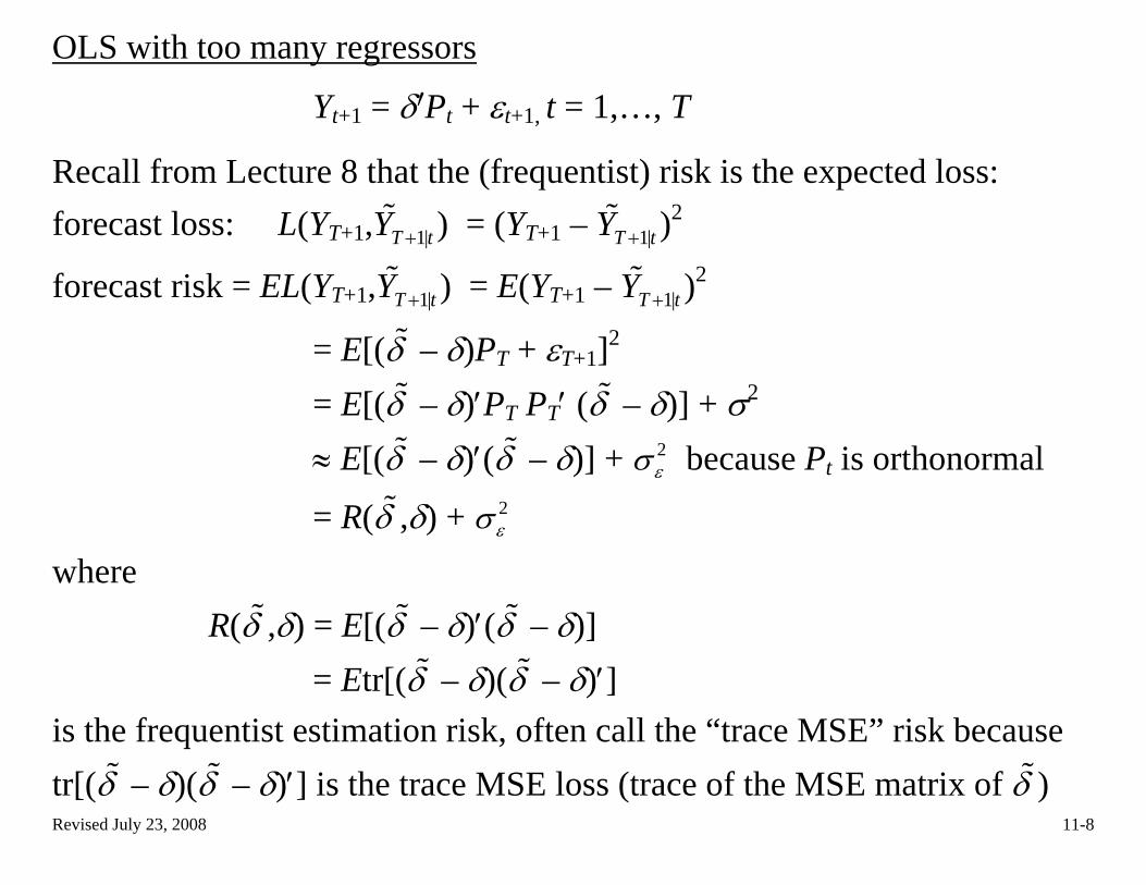
OLS with too many regressors

Yt+1 = δ′Pt + εt+1, t = 1,…, T

Recall from Lecture 8 that the (frequentist) risk is the expected loss: forecast loss: L(YT+1, t1|TY + ) = (YT+1 – 1|T tY + )2

forecast risk = EL(YT+1, t1|TY + ) = E(YT+1 – 1|T tY + )2

= E[(δ – δ)PT + εT+1]2

= E[(δ – δ)′PT PT′ (δ – δ)] + σ2 ≈ E[(δ – δ)′(δ – δ)] + 2

εσ because Pt is orthonormal

= R(δ ,δ) + 2εσ

where R(δ ,δ) = E[(δ – δ)′(δ – δ)]

= Etr[(δ – δ)(δ – δ)′] is the frequentist estimation risk, often call the “trace MSE” risk because tr[(δ – δ)(δ – δ)′] is the trace MSE loss (trace of the MSE matrix of δ ) Revised July 23, 2008 11-8

OLS with too many regressors, ctd


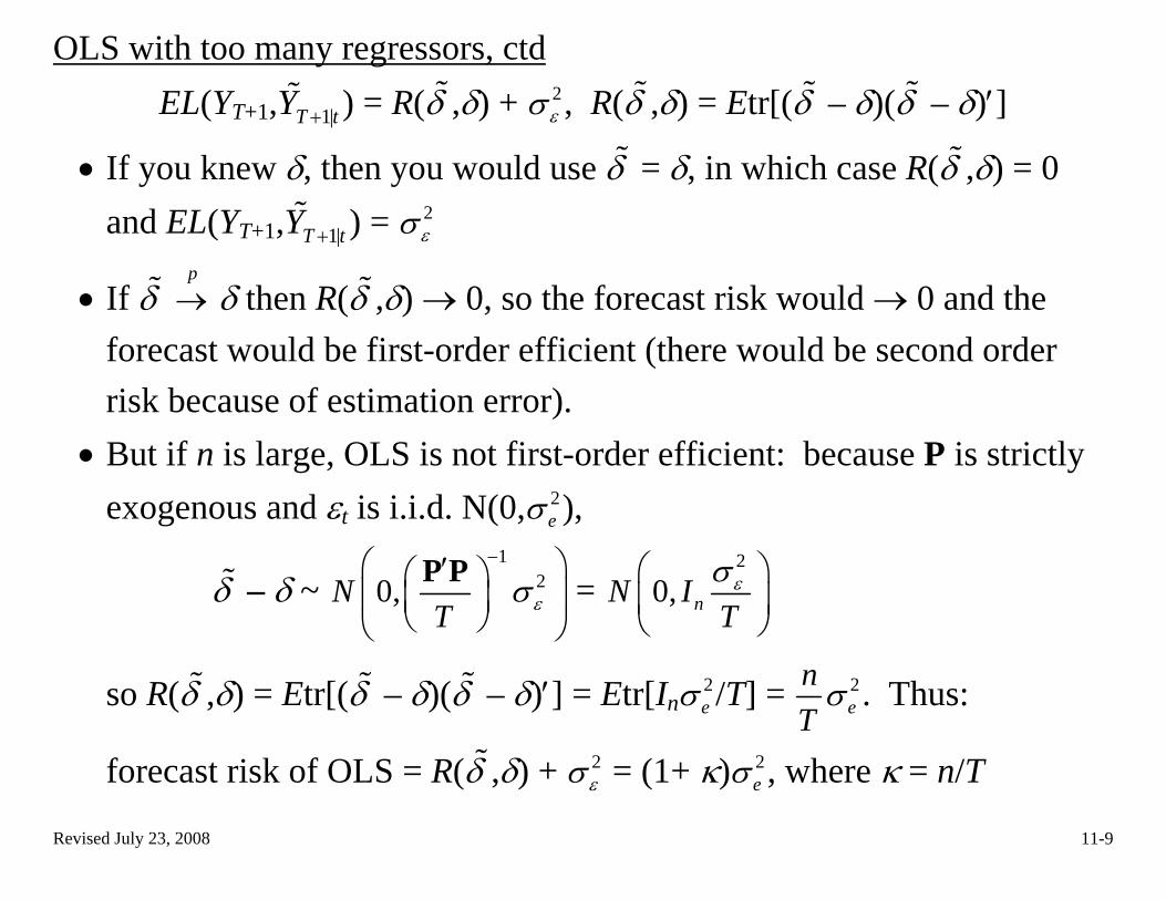
EL(YT+1, t ) = R(1|TY + δ ,δ) + 2εσ , R(δ ,δ) = Etr[(δ – δ)(δ – δ)′]

• If you knew δ, then you would use δ = δ, in which case R(δ ,δ) = 0 and EL(YT+1, t ) = 1|TY +

2εσ

• If δ δ then R(p→ δ ,δ) → 0, so the forecast risk would → 0 and the

forecast would be first-order efficient (there would be second order risk because of estimation error).

• But if n is large, OLS is not first-order efficient: because P is strictly exogenous and εt is i.i.d. N(0, 2

eσ ),

δ – δ ~ 1

20,NT εσ

−⎛ ⎞′⎛ ⎞⎜ ⎟⎜ ⎟

⎝ ⎠⎝ ⎠

P P = 2

0, nN ITεσ⎛ ⎞

⎜ ⎟⎝ ⎠

so R(δ ,δ) = Etr[(δ – δ)(δ – δ)′] = Etr[In2eσ /T] = n

T2eσ . Thus:

forecast risk of OLS = R(δ ,δ) + 2εσ = (1+ κ) 2

eσ , where κ = n/T

OLS with too many regressors, ctd OLS forecast risk: EL(YT+1, t


1|TY + ) = (1+ κ) , where κ = n/T > 2eσ

2eσ

• If κ ≈ 0, OLS is nearly first order efficient. Parsimony! • If n/T is large, this result provides a theory to support your intuition:

OLS doesn’t achieve first-order forecast efficiency • Moreover, if n ≥ 3, OLS isn’t admissible under trace MSE loss (Stein

(1955)): there exists an estimator δ with frequentist risk R(δ ,δ) that dominate OLS (risk at least as good as OLS for some δ, and no worse for all δ). James and Stein (1960) constructed a shrinkage estimator that dominates OLS (does better than OLS near δ = 0).

• Things that don’t achieve first order forecast efficiency: o throwing out all but a few regressors (throw away information!) o keeping only the statistically significant regressors o choosing regressors by information criteria (AIC or BIC)

The blessing of dimensionality, part 1 We can do better than OLS. Recall the forecasting risk is R(δ ,δ) + 2

εσ .

We can do nothing about 2εσ , but R(δ ,δ) depends on the estimator used so

the choice of estimator can reduce R(δ ,δ). Setup • Adopt a local nesting in which δi = di/ T (else there would be an R2 =

1 forecasting regression in the limit – this keeps the regression ESS from exploding as we let T → ∞)

• Let {di} have the empirical cdf Gn (suppose you observed {di} – just construct the empirical cdf of {di}, that is Gn)

• Consider only estimators that (sensibly) produce the same forecast no matter how you order the regressors (“permutation equivariant”)


The blessing of dimensionality, part 1, ctd. Frequentist risk for permutation equivariant estimators:

R(δ ,δ) = )2

1

(n

i ii

E δ δ=

−∑ (trace MSE loss)

= 1 2) (because δi = di/1

(n

i ii

nT

n E d d−

=

⎛ ⎞⎜ ⎟⎝ ⎠

−∑ T )

= ) (permutation equivariance & cdf Gn) 2( ) (nE d d dG dκ −∫ = κ ) (Bayes risk* of estimator wrt Gn) (

nGr d d

where κ = n/T. Thus the frequentist risk for permutation equivariant estimators is the Bayes risk with respect to the empirical cdf of the d’s, Gn. *Recall from Lecture 8 that the Bayes risk )(

nGR d is the expectation of the

frequentist risk, with respect to a prior distribution


The blessing of dimensionality, part 1, ctd.

R(δ ,δ) = 2

1

( )n

i ii

E δ δ=

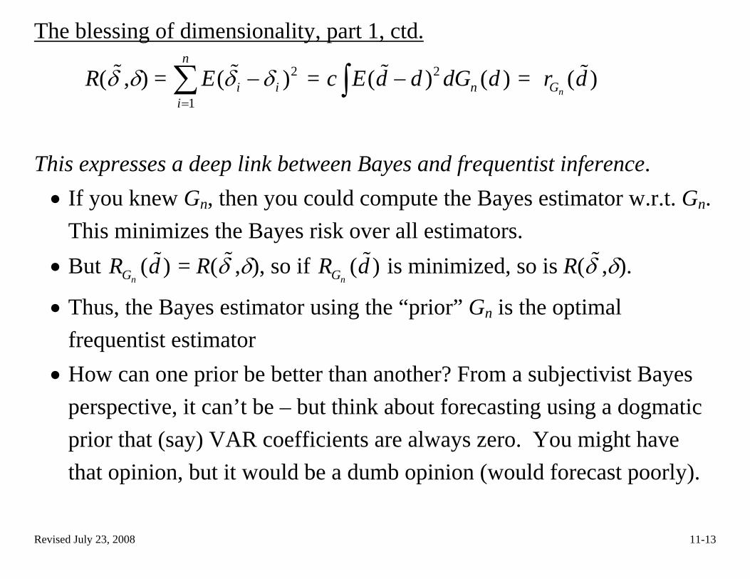
−∑ = )2( ) (nc E d d dG d−∫ = ( )nGr d

This expresses a deep link between Bayes and frequentist inference. • If you knew Gn, then you could compute the Bayes estimator w.r.t. Gn.

This minimizes the Bayes risk over all estimators. • But ( )

nGR d = R(δ ,δ), so if ( )nGR d is minimized, so is R(δ ,δ).

• Thus, the Bayes estimator using the “prior” Gn is the optimal frequentist estimator

• How can one prior be better than another? From a subjectivist Bayes perspective, it can’t be – but think about forecasting using a dogmatic prior that (say) VAR coefficients are always zero. You might have that opinion, but it would be a dumb opinion (would forecast poorly).


The blessing of dimensionality, part 1, ctd. The Empirical Bayes estimator uses the data to pick the prior

Books on Empirical Bayes: Maritz and Lwin (1989), Carlin and Louis (1996), and Lehmann and Casella (1998, Section 4.6).

Frequentist: minδ r (nG d ) = 2( ) ( )nE d d dG dκ −∫ cdf of di

Bayes: minδ r (G d ) = )2( ) (E d d dG dκ −∫ subjective prior


Empirical Bayes: minδ r (d ) = )2 ˆ( ) (E d d dG dκ −∫ estimated “prior” G

• Under technical conditions, the Empirical Bayes estimator is asymptotically admissible and asy. optimal (Robbins (1964))

• James-Stein (1960) is Empirical Bayes (Efron and Morris (1973)) • EB has certain minimax properties (Zhang (2003, 2005)) • can be nonparametric or parametric G• asymptotically, EB is minimum risk equivariant (Edelman (1988),

Knox, Stock, Watson (2001) for regression)


The blessing of dimensionality, part 1, ctd. These are great results, but they have not been proven in time series contexts with predetermined predictors. However they are still useful guides. They tell us: • Shrinkage (Bayes) methods can produce good forecasts (from a

frequentist risk perspective) with many predictors • Bayes methods with tuned (estimated) parameters are particularly

appealing • Forecasts using many predictors can outperform forecasts using no or

only a few predictors. • AIC, etc is not the optimal thing to do.

We will return to these methods – some theory, some empirical results.


The blessing of dimensionality, part 2 The second example is estimation of factors in a dynamic factor model

(Geweke (1977), Sargent and Sims (1977)). Suppose the n variables in Xt are related to some unobserved factors Ft, which evolve according to a time series process:

Xt = ΛFt + et Ft = Φ(L)Ft–1 + Gηt,

If the factors were observed they could be very useful for forecasting, but they aren’t observed.

The original approach to this problem (Engle and Watson (1981),

Stock and Watson (1989, 1991), Sargent (1989), Quah and Sargent (1993)) was to fit the two equations above by ML using the Kalman filter. But the proliferation of parameters and computational limitations of ML in high dimensions limited this approach to small n.

The blessing of dimensionality, part 2, ctd. How could many series be a blessing? Geweke (discussing Quah and

Sargent (1993)) suggested that many series could improve estimates of Ft considerably.

An example following Forni and Reichlin (1998). Suppose Ft is

scalar so Λ is a vector with elements λi so Xit = λift + eit

Then 1

1 n

iti

Xn =∑ = ( )

1

1 n

i t iti

F en

λ=

+∑ = 1 1

1 1n n

i t it


i i

F en n

λ= =

⎛ ⎞ +⎜ ⎟⎝ ⎠∑ ∑

If the errors uit have limited dependence across series, then as n gets large,

1

1 n

iti

Xn =∑

p→ λ Ft

In this special case, a very easy nonparametric estimate (the cross-sectional average) is able to recover Ft – as long as n is large!


From curse to blessing • All the procedures below are justified using asymptotic theory for

large n by assuming that n → ∞, usually at some rate relative to T . Often n2/T is treated as large in the asymptotics; this makes sense in an application with T = 160 and n = 100, say.

• By having large n, procedures (more sophisticated than the simple

average in the previous example) are available for consistent estimation of tuning priors (prior hyperparameters) in forecasting and for factors in DFMs.

• Most of the theory, and all of the empirical work, has been developed

within the past 10-12 years.


Outline 1) Why Might You Want To Use Hundreds of Series? 2) Dimensionality: From Curse to Blessing 3) Dynamic Factor Models: Specification and Estimation 4) Other High-Dimensional Forecasting Methods 5) Empirical Performance of High-Dimensional Methods 6) SVARs with Factors: FAVAR 7) Factors as Instruments 8) DSGEs and Factor Models


3) Dynamic Factor Models: Specification and Estimation (A) Specification: The DFM, the Static Form, and the Approximate DFM

The idea (conjecture) behind DFMs is that small number of factors captures the covariation in macro time series (Geweke (1977), Sargent and Sims (1977)). The exact DFM Xit = λi(L)ft + eit, i = 1,…,n,

Ψ(L)ft = ηt, where: ft = q unobserved “dynamic factors”

λi(L)ft = “common component” λi(L) = “dynamic factor loadings” lag polynomial eit = idiosyncratic disturbance cov(ft, eis) = 0 for all i, s

Eeitejs = 0, i ≠ j, for all t, s (exact DFM)

The exact DFM, ctd.

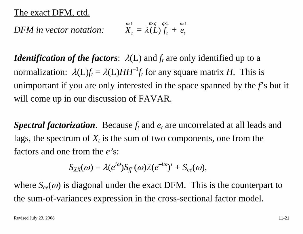
DFM in vector notation: 1n

tX×

= ( )n qLλ× 1

t

qf×

+ 1n

te×

Identification of the factors: λ(L) and ft are only identified up to a normalization: λ(L)ft = λ(L)HH–1ft for any square matrix H. This is unimportant if you are only interested in the space spanned by the f’s but it will come up in our discussion of FAVAR. Spectral factorization. Because ft and et are uncorrelated at all leads and lags, the spectrum of Xt is the sum of two components, one from the factors and one from the e’s:

SXX(ω) = λ(eiω)Sff (ω)λ(e–iω)′ + See(ω),

where See(ω) is diagonal under the exact DFM. This is the counterpart to the sum-of-variances expression in the cross-sectional factor model.



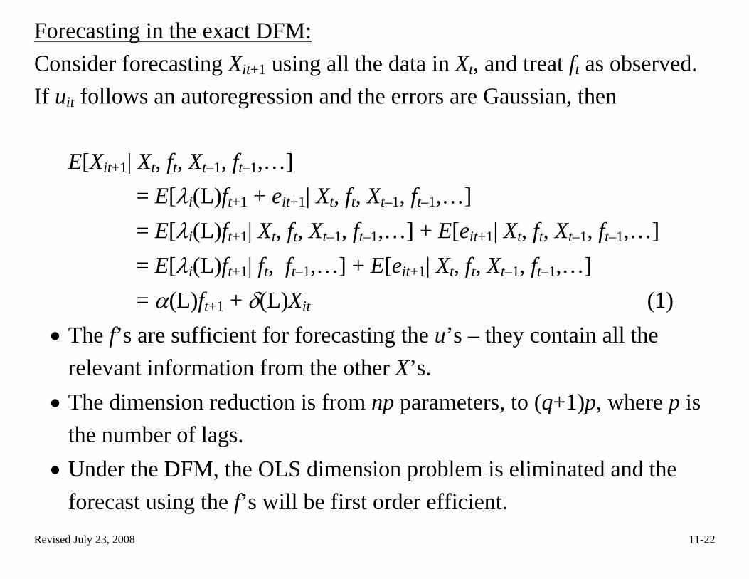
Forecasting in the exact DFM: Consider forecasting Xit+1 using all the data in Xt, and treat ft as observed. If uit follows an autoregression and the errors are Gaussian, then

E[Xit+1| Xt, ft, Xt–1, ft–1,…] = E[λi(L)ft+1 + eit+1| Xt, ft, Xt–1, ft–1,…] = E[λi(L)ft+1| Xt, ft, Xt–1, ft–1,…] + E[eit+1| Xt, ft, Xt–1, ft–1,…] = E[λi(L)ft+1| ft, ft–1,…] + E[eit+1| Xt, ft, Xt–1, ft–1,…] = α(L)ft+1 + δ(L)Xit (1)

• The f’s are sufficient for forecasting the u’s – they contain all the relevant information from the other X’s.

• The dimension reduction is from np parameters, to (q+1)p, where p is the number of lags.

• Under the DFM, the OLS dimension problem is eliminated and the forecast using the f’s will be first order efficient.


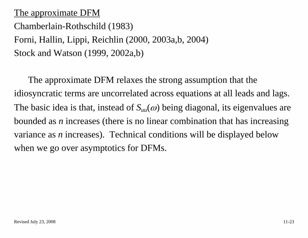
The approximate DFM Chamberlain-Rothschild (1983) Forni, Hallin, Lippi, Reichlin (2000, 2003a,b, 2004) Stock and Watson (1999, 2002a,b)

The approximate DFM relaxes the strong assumption that the idiosyncratic terms are uncorrelated across equations at all leads and lags. The basic idea is that, instead of Suu(ω) being diagonal, its eigenvalues are bounded as n increases (there is no linear combination that has increasing variance as n increases). Technical conditions will be displayed below when we go over asymptotics for DFMs.

The Static Form of the DFM The DFM Xt = λ(L)ft + et where Ψ(L)ft = ηt, Suppose that λ(L) has at most pf lags. Then the DFM can be written,

1t

nt

X

X

⎛ ⎞⎜ ⎟⎜ ⎟⎜ ⎟⎝ ⎠

= 10 1

0

f

f

p

n np

λ λ

λ λ

⎛ ⎞⎜ ⎟⎜ ⎟⎜ ⎟⎝ ⎠

…

f

t

t p

f

f −

⎛ ⎞⎜ ⎟⎜ ⎟⎜ ⎟⎝ ⎠

+ 1t

nt

e

e

⎛ ⎞⎜ ⎟⎜ ⎟⎜ ⎟⎝ ⎠

or = 1n

tX× n r×

Λ 1r

tF×

+ 1n

te×

where the number of static factors, r, could be as much as qpf. Ft is the vector of static factors. The VAR for ft implies that there is a VAR for Ft:

Φ(L)Ft = Gηt where G is a matrix of 1’s and zeros and Φ consists of 1’s, 0’s, and Ψ’s.


(B) Estimation: MLE, Principal Components, and Generalized PC MLE Engle-Watson (1981); Stock and Watson (1989), Sargent (1989) Suppose Ft follows a VAR(1). The DFM in static form is: Ft = ΦFt–1 + Gηt (VAR(1) assumption)

Xt = ΛFt + et Suppose that eit follow individual AR’s, written in first order form:

te = D 1te − + Hζt where ζt is n × 1, H = [In | 0]′, pe is the number of lags in the eit AR’s, and

= (et′, et-1′,…, ′)′. Combining the Ft and equations yields: te 1et pe − + te


MLE, ctd. The DFM in state space form:

t

t

Fe

⎛ ⎞⎜ ⎟⎝ ⎠

= 0

0 DΦ⎛ ⎞⎜ ⎟⎝ ⎠

⎛ ⎞⎜ ⎟⎝ ⎠

1

1

t

t

Fe

−

−

+ 0

0G

H⎛ ⎞⎜ ⎟⎝ ⎠

t

t

ηζ⎛ ⎞⎜ ⎟⎝ ⎠

(2)

Xt = ( )0 0nIΛ⎡⎣⎛⎤⎦

t

t

Fe⎞

⎜ ⎟⎝

(3) ⎠

• Equation (2) is the state transition equation and equation (3) is the observer equation in the state space formulation of the DFM. The quasi-likelihood can now be computed using the Kalman filter.

• Early implementations used the MLE to estimate models with a single dynamic factor (r=1) with only a handful of variables: Engle-Watson (1981) Sargent (1989): estimate early DSGE Stock-Watson (1989): coincident index Quah-Sargent (1993) – more variables but a special structure



MLE, ctd. • Historically, computation got too hard as n increased beyond a half-

dozen variables (and the model was kept general), so other (nonparametric) methods were developed.

• However, there have been recent advances that make the MLE more practical: 1) Computation

a) faster computers b) can get very good starting values (specifics discussed next) c) new KF speedup: Jungbacker and Koopman (2008)

2) Theory: Doz, Giannone, and Reichlin (2006)

3) Empirical experience (discussed below): Doz, Giannone, and Reichlin (2006) Reiss and Watson (2008)


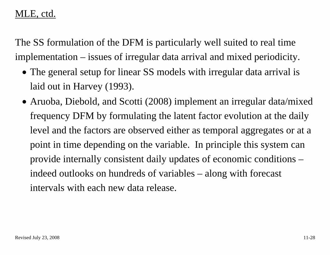
MLE, ctd. The SS formulation of the DFM is particularly well suited to real time implementation – issues of irregular data arrival and mixed periodicity. • The general setup for linear SS models with irregular data arrival is

laid out in Harvey (1993). • Aruoba, Diebold, and Scotti (2008) implement an irregular data/mixed

frequency DFM by formulating the latent factor evolution at the daily level and the factors are observed either as temporal aggregates or at a point in time depending on the variable. In principle this system can provide internally consistent daily updates of economic conditions – indeed outlooks on hundreds of variables – along with forecast intervals with each new data release.

Estimation by Principal Components DFM in static form: Xt = ΛFt + et By analogy to regression, consider estimating Λ and {Ft} by NLLS:

1

1,..., ,

1

min ( ) '( )T

T

F F t t t tt

T X F X F−Λ

=

− Λ −∑ Λ

subject to Λ′Λ = Ir (identification). Now concentrate out {Ft}, given Λ:

minΛ 1 11

[ ( ) ]Tt tt

T X I X− −=

′ ′− Λ Λ Λ Λ∑

⇔ maxΛ 1 11

( )Tt tt

T X X− −=

′ ′Λ Λ Λ Λ∑

⇔ maxΛ tr{(Λ′Λ)–1/2′ Λ′( )11

Tt tt

T X−=

X ′∑ Λ(Λ′Λ)–1/2}

⇔ maxΛ Λ′ ˆXXΣ Λ s.t. Λ′Λ = Ir, where ˆ

XXΣ = X11

Tt tt

T X−=

′∑

⇒ = first r eigenvectors of Λ ˆXXΣ

⇒ = tF ˆtX′Λ = first r principal components of Xt.


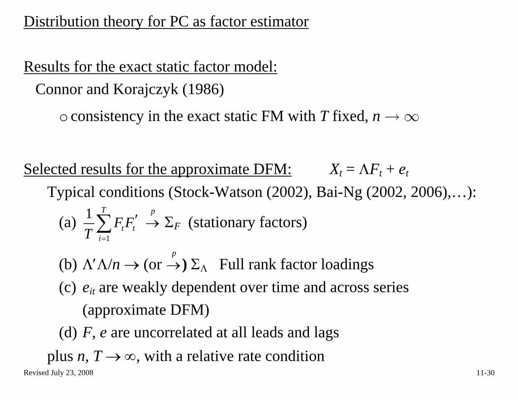
Distribution theory for PC as factor estimator Results for the exact static factor model:

Connor and Korajczyk (1986)

o consistency in the exact static FM with T fixed, n → ∞

Selected results for the approximate DFM: Xt = ΛFt + et

Typical conditions (Stock-Watson (2002), Bai-Ng (2002, 2006),…):

(a) 1

1 T

t ti

F FT =

′∑ ΣF (stationary factors) p→

(b) Λ′Λ/n → (or ) ΣΛ Full rank factor loadings p→

(c) eit are weakly dependent over time and across series (approximate DFM)

(d) F, e are uncorrelated at all leads and lags plus n, T → ∞, with a relative rate condition


Selected results for the approximate DFM, ctd. Stock and Watson (2002a)

o consistency in the approximate DFM, n, T →∞, no n/T restrictions

o justify using as a regressor without adjustment tF

Bai and Ng (2006)

o N2/T → ∞ (Think about this – not the principle of parsimony!) o asymptotic normality of PCA estimator of the common component

at rate min(n1/2, T1/2) in approximate DFM o improve upon Stock-Watson (2002a) rate for using as a

regressor tF

o Method for constructing confidence bands for predicted value (these are for predicted value – not forecast confidence bands)



PC estimation in the approximate DFM, ctd. • Data irregularities probably are best handled parametrically in the SS

setup using the KF • However the PC algorithm can be modified for data irregularities

including mixed frequency data, see Stock and Watson (2002b, Appendix).

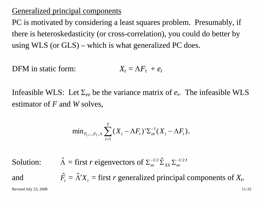
Generalized principal components PC is motivated by considering a least squares problem. Presumably, if there is heteroskedasticity (or cross-correlation), you could do better by using WLS (or GLS) – which is what generalized PC does. DFM in static form: Xt = ΛFt + et Infeasible WLS: Let Σee be the variance matrix of et. The infeasible WLS estimator of F and W solves,

1

1,..., ,

1

min ( ) ' ( )T

T

F F t t ee t tt

X F X F−Λ

=

− Λ Σ − Λ∑ .

Solution: = first r eigenvectors of Λ 1/2ee−Σ ˆ

XXΣ 1/2ee−Σ ′

and = tF ˆtX′Λ = first r generalized principal components of Xt.


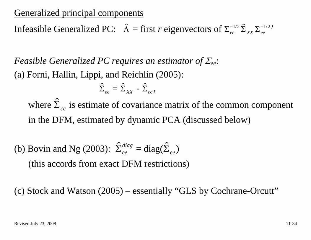
Generalized principal components

Infeasible Generalized PC: Λ = first r eigenvectors of 1/2ee−Σ ˆ

XXΣ 1/2ee−Σ ′

Feasible Generalized PC requires an estimator of Σee: (a) Forni, Hallin, Lippi, and Reichlin (2005):

ˆ ˆ ˆeeΣ = XXΣ - ccΣ ,

where is estimate of covariance matrix of the common component in the DFM, estimated by dynamic PCA (discussed below)

ˆccΣ

(b) Bovin and Ng (2003): ˆ diag

eeΣ = diag( ˆeeΣ )

(this accords from exact DFM restrictions) (c) Stock and Watson (2005) – essentially “GLS by Cochrane-Orcutt”


Forecasting with estimated factors Comments: 1. The basic idea – using factors as predictors. Suppose the object is to

forecast Xit using estimated factors. According to the exact DFM theory, the (first order) optimal forecast is obtained from the regression in (1). The dynamic factors aren’t observed, so this leads to the regression,

Xit+1 = α(L) + δ(L)Xit + ζt+1 tF

In some cases you might think some other variables Wt are good predictors so you could augment this:

ˆXit+1 = α(L) + δ(L)Xit + γ(L)Wt + ζt+1 tF

If the number of regressors is small, this will yield first-order optimal forecasts.


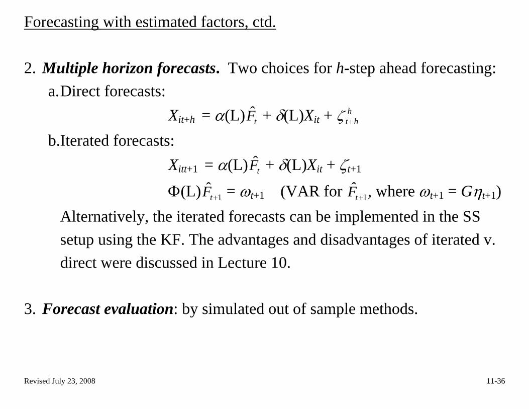
Forecasting with estimated factors, ctd. 2. Multiple horizon forecasts. Two choices for h-step ahead forecasting:

a. Direct forecasts: Xit+h = α(L) + δ(L)Xit + htF h

tζ + b.Iterated forecasts:

Xitt+1 = α(L) + δ(L)Xit + ζt+1 tF

Φ(L) 1tF + = ωt+1 (VAR for 1tF + , where ωt+1 = Gηt+1) Alternatively, the iterated forecasts can be implemented in the SS setup using the KF. The advantages and disadvantages of iterated v. direct were discussed in Lecture 10.

3. Forecast evaluation: by simulated out of sample methods.


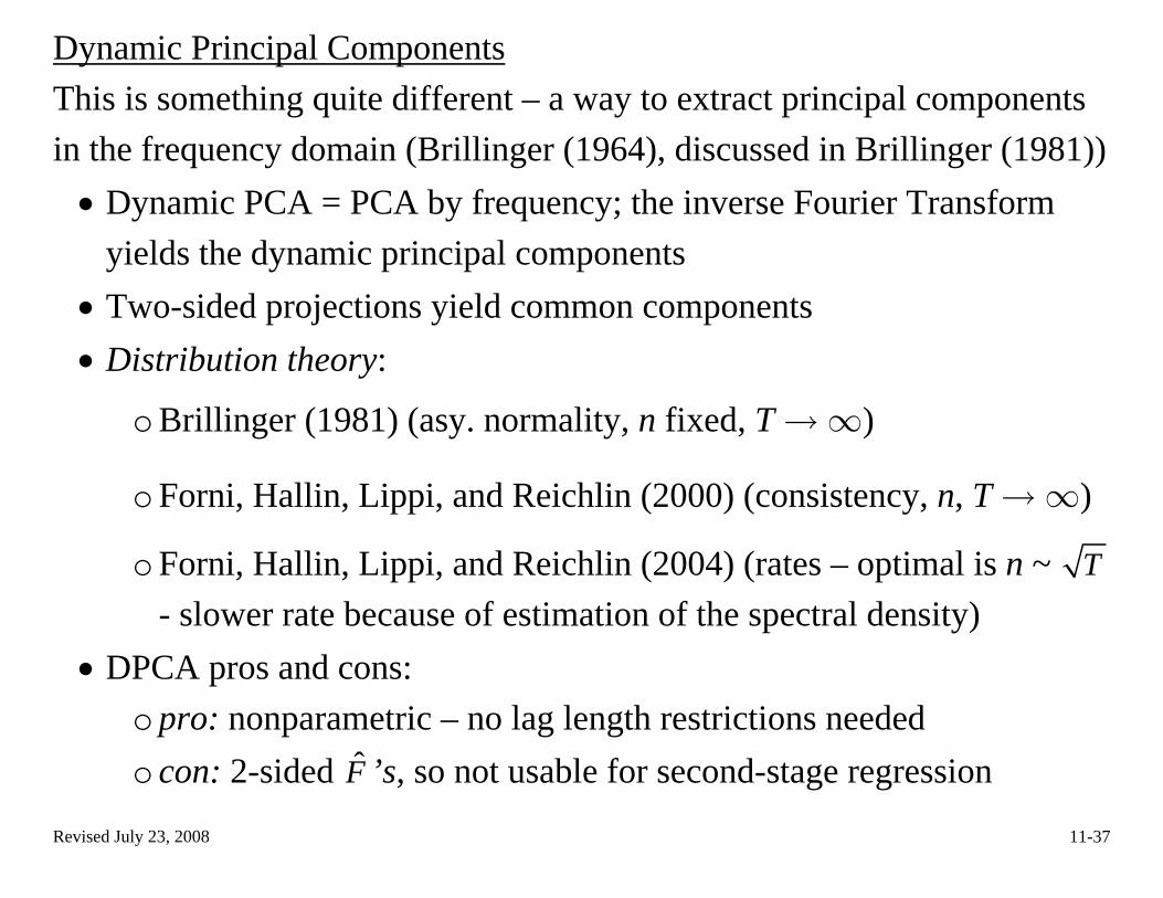
Dynamic Principal Components This is something quite different – a way to extract principal components in the frequency domain (Brillinger (1964), discussed in Brillinger (1981)) • Dynamic PCA = PCA by frequency; the inverse Fourier Transform

yields the dynamic principal components • Two-sided projections yield common components • Distribution theory:

o Brillinger (1981) (asy. normality, n fixed, T → ∞)

o Forni, Hallin, Lippi, and Reichlin (2000) (consistency, n, T → ∞)

o Forni, Hallin, Lippi, and Reichlin (2004) (rates – optimal is n ~ T - slower rate because of estimation of the spectral density)

• DPCA pros and cons: o pro: nonparametric – no lag length restrictions needed

ˆo con: 2-sided ’s, so not usable for second-stage regression F



Which estimator to use – MLE, PC, or Generalized PC? (a) Theoretical results ranking MLE, PC, and Generalized PC Choi (2007) compares asymptotic variances of PC (derived by Bai (2003)) and Generalized PC, using the full covariance matrix of et|(F1,…,FT) (GLS, not WLS). Choi finds asymptotic gains for GPC (smaller variance of the asymptotic distribution for infeasible GPC than PC)). Given the parameters, the KF estimator of Ft is the optimal estimator of Ft if the errors are Gaussian; for nonGaussian errors, the KF estimator is the MMSE estimator. This doesn’t take parameter estimation error into account.

(b) Simulation evidence • Choi (2007) compares PC, infeasible GLS-GPC, and feasible GLS-GPC

in a MC study. He finds efficiency gains for feasible GPC in some cases, however the estimation of Σ hurts performance relative to infeasible GLS (Σ known), so feasible GPC improves on PC in some but not all cases. No evidence on full MLE.

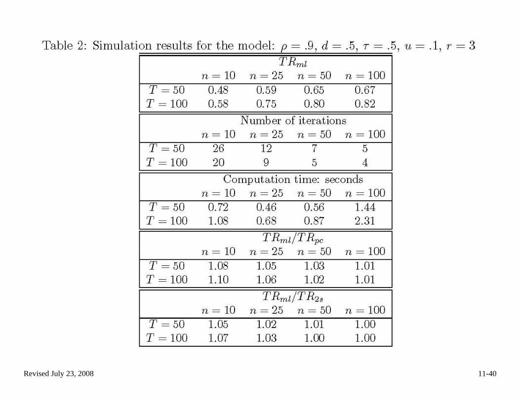
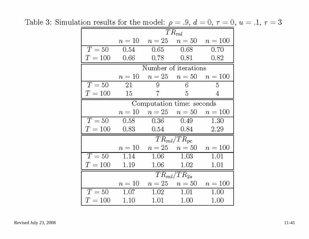
• Doz, Giannone, and Reichlin (2006) MC study of: o PC o PC, estimation of DFM parameters using PC estimates, then a

single pass of the Kalman Filter (Giannone, Reichlin, and Sala (2004))

o ML (PC for starting values, then use EM algorithm to convergence)

Doz, Giannone, and Reichlin (2006) results for ( )

( )

1ˆ ˆ ˆ ˆ( )tr F F F F F F

tr F F

−′ ′ ′

′



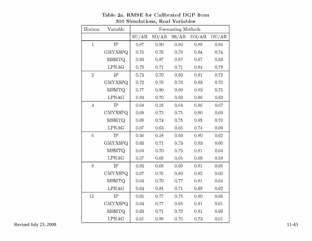
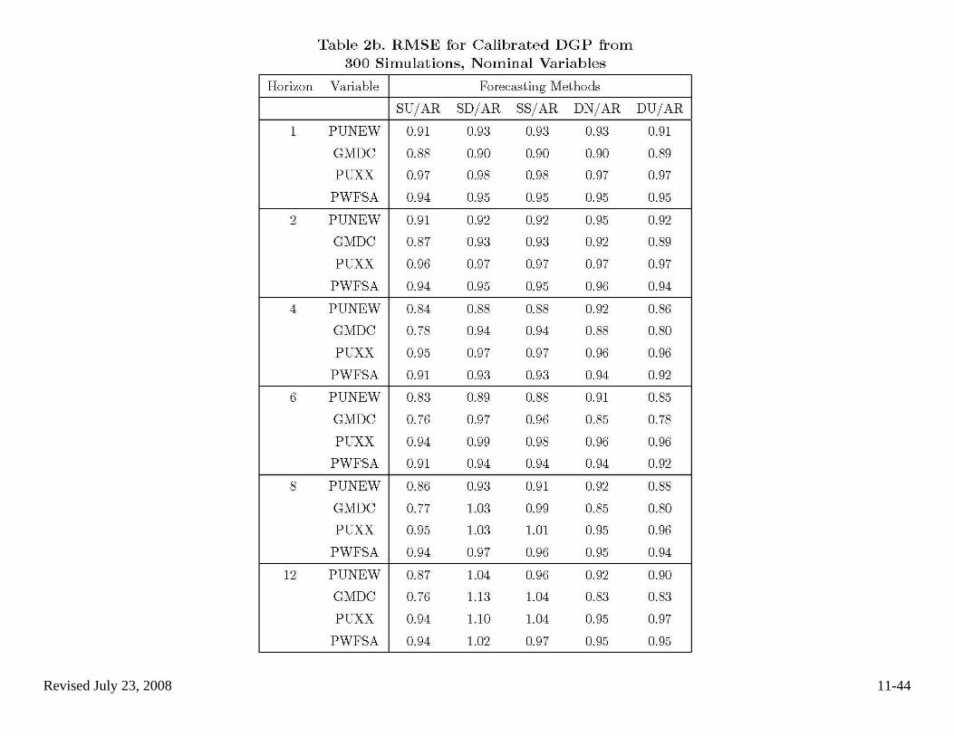
(b) Simulation evidence, ctd • Boivin-Ng (2005) compare combinations of factor estimation methods

and forecasting equation specifications, from the perspective of forecast MSE.

o Of interest here is their comparison of PC (S, for static) to GPC (D, for dynamic)

o The design in the following figures was calibrated to a large US macro data set

o They report RMSE ratios, relative to an AR benchmark the columns to compare are the “S” (PC) to “D” (GPC) columns

o Their conclusion is that PC generally works best.


(c) Empirical evidence (i) Comparisons of forecasts – actual data sets (US, EU): • Stock & Watson, Handbook of Economic Forecasting (2006) plus

extensive empirical work as backup – empirical forecasting comparison over many series

• D’Agostino and Giannone (2006) • Marcellino and coauthors (several) • Broad summary of findings across papers:

o PC, WLS-PC, and GLS-PC have very similar performance. o GLS-PC can produce modest outliers (sometimes better,

sometimes worse) o mild preference for PC


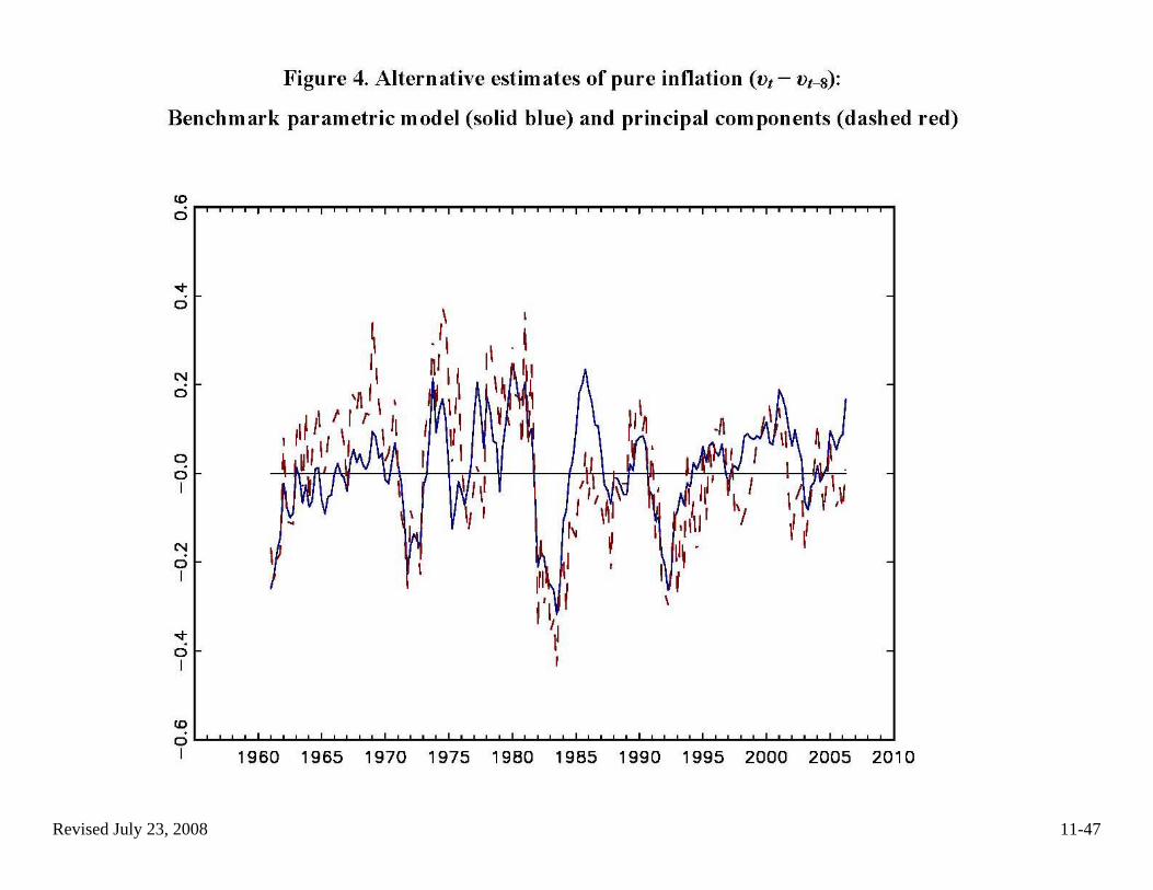
(c) Empirical evidence, ctd (ii) A bit of filtering evidence • Riess and Watson (2007)

o application in which the factor structure is weak (prices with large idiosyncratic terms – lots of idiosyncratic movement + measurement error)

o PC estimate of factors vs. MLE from the KF – take a look!


Which estimator to use? • For forecasting, it doesn’t seem to matter much – PC seems to work as

well as the others in typical applications • MLE is appealing theoretically and has the additional advantage of

temporal smoothing – this might be the most promising avenue currently.

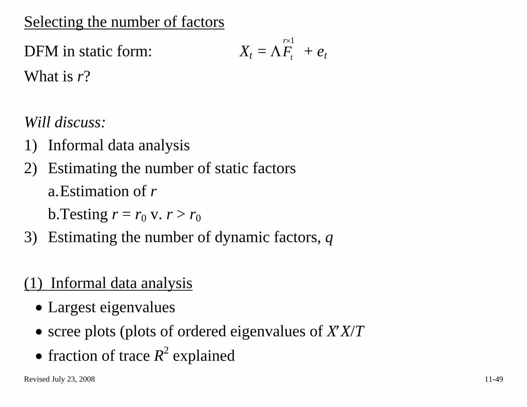
Selecting the number of factors

DFM in static form: Xt = Λ1r

tF×

+ et What is r? Will discuss: 1) Informal data analysis 2) Estimating the number of static factors

a. Estimation of r b.Testing r = r0 v. r > r0

3) Estimating the number of dynamic factors, q (1) Informal data analysis • Largest eigenvalues • scree plots (plots of ordered eigenvalues of X′X/T • fraction of trace R2 explained


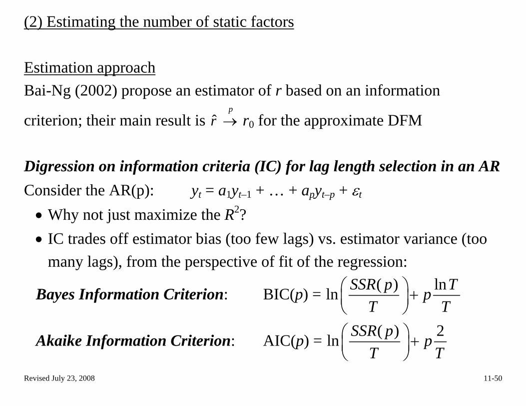
(2) Estimating the number of static factors Estimation approach Bai-Ng (2002) propose an estimator of r based on an information

criterion; their main result is r0 for the approximate DFM rp→

Digression on information criteria (IC) for lag length selection in an AR Consider the AR(p): yt = a1yt–1 + … + apyt–p + εt • Why not just maximize the R2? • IC trades off estimator bias (too few lags) vs. estimator variance (too

many lags), from the perspective of fit of the regression:

Bayes Information Criterion: BIC(p) = ( ) lnln SSR p TpT T

⎛ ⎞ +⎜ ⎟⎝ ⎠

Akaike Information Criterion: AIC(p) = ( ) 2ln SSR p pT T

⎛ ⎞ +⎜ ⎟⎝ ⎠


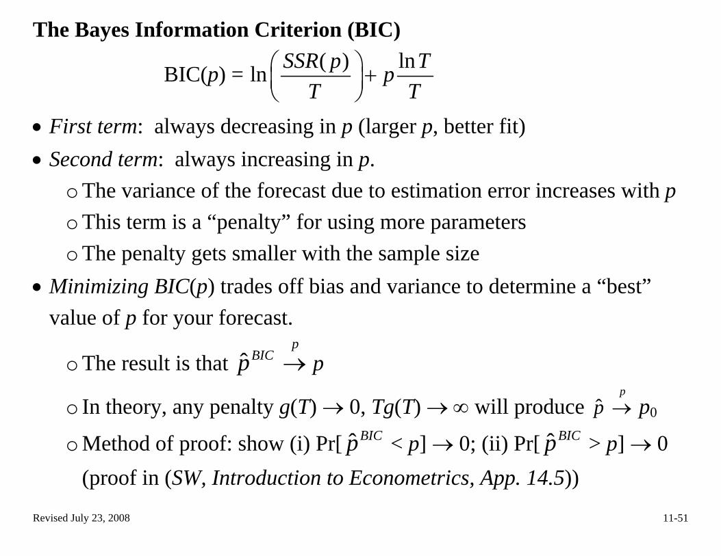
The Bayes Information Criterion (BIC)

BIC(p) = ( ) lnln SSR p TpT T

⎛ ⎞ +⎜ ⎟⎝ ⎠

• First term: always decreasing in p (larger p, better fit) • Second term: always increasing in p.

o The variance of the forecast due to estimation error increases with p o This term is a “penalty” for using more parameters o The penalty gets smaller with the sample size

• Minimizing BIC(p) trades off bias and variance to determine a “best” value of p for your forecast.

o The result is that ˆ BICp p p→

o In theory, any penalty g(T) → 0, Tg(T) → ∞ will produce p0 p→p

o Method of proof: show (i) Pr[ ˆ BICp < p] → 0; (ii) Pr[ ˆ BICp > p] → 0 (proof in (SW, Introduction to Econometrics, App. 14.5))


The Akaike Information Criterion (AIC)

AIC(p) = ( ) 2ln SSR p pT T

⎛ ⎞ +⎜ ⎟⎝ ⎠

BIC(p) = ( ) lnln SSR p TpT T

⎛ ⎞ +⎜ ⎟⎝ ⎠

The penalty term is smaller for AIC than BIC (2 < lnT)

o AIC estimates more lags (larger p) than the BIC o In fact, the AIC estimator of p isn’t consistent – it can overestimate

p – the penalty isn’t big enough: for AIC, Tg(T) = T× (2/T) = 2, but you need Tg(T) → ∞ for consistency.

o Still, AIC might be desirable if you want to err on the side of long lags



Example: AR model of U.S. Δinflation, lags 0 – 6:

# Lags BIC AIC R2

0 1.095 1.076 0.000 1 1.067 1.030 0.056 2 0.955 0.900 0.181 3 0.957 0.884 0.203 4 0.986 0.895 0.204 5 1.016 0.906 0.204 6 1.046 0.918 0.204

• BIC chooses 2 lags, AIC chooses 3 lags. • If you used the R2 to enough digits, you would (always) select the

largest possible number of lags.

Estimating the number of static factors, ctd. The Bai-Ng (2002) information criteria have the same form:

IC(r) = ( )ln SSR rT

⎛ ⎞⎜ ⎟ + penalty(N, T, r) ⎝ ⎠

Bai-Ng (2002) propose several IC’s with different penalty factors that all produce consistent estimators of k. Here is the one that seems to work best in MCs (and is the most widely used in empirical work):

ICp2(r) = ln(V(r, )) + ˆ rF [ ]ln min( , )N Tr N TNT+⎛ ⎞

⎜ ⎟⎝ ⎠

where V(r, ) = minΛˆ rF ( )2

1 1

1 ˆN T

r rit i t

i t

X FNT

λ= =

′−∑∑

ˆ rtF are the PC estimates of r factors

(minor notational note: Bai-Ng (2002) use proxy argument k, not r)


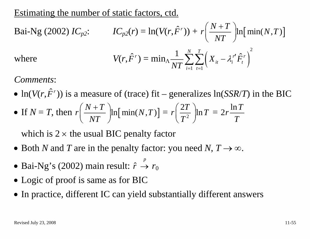
Estimating the number of static factors, ctd.

Bai-Ng (2002) ICp2: ICp2(r) = ln(V(r, )) + ˆ rF [ ]ln min( , )N Tr N TNT+⎛ ⎞

⎜ ⎟⎝ ⎠

where V(r, ) = minΛˆ rF ( )2

1 1

1 ˆN T

r rit i t

i t

X FNT

λ= =

′−∑∑

Comments: ˆ• ln(V(r, )) is a measure of (trace) fit – generalizes ln(SSR/T) in the BIC rF

• If N = T, then [ ]ln min( , )N Tr N TNT+⎛ ⎞

⎜ ⎟⎝ ⎠

= 2

2 lnTr TT

⎛ ⎞⎜ ⎟⎝ ⎠

= ln2 TrT

which is 2 × the usual BIC penalty factor • Both N and T are in the penalty factor: you need N, T → ∞.

• Bai-Ng’s (2002) main result: r0 r

• Logic of proof is same as for BIC

p→

• In practice, different IC can yield substantially different answers


(3) Estimating the number of dynamic factors, q Bai-Ng consider estimating the number of static factors – which is directly useful for forecasting using PC. For the MLE (which specifies a process for the dynamic factors) it is desirable to estimate the number of dynamic factors. Recall that the static factors are constructed by stacking the dynamic factors:

Ft =

f

t

t p

f

f −

⎛ ⎞⎜ ⎟⎜ ⎟⎜ ⎟⎝ ⎠

so the static factors must be dynamically singular: the rank of the innovation variance matrix in the projection of Ft on Ft–1 must be the rank of (the spectrum of) ft (since many of the elements of Ft are perfectly predictable from Ft–1) Revised July 23, 2008 11-56

Estimating the number of dynamic factors, ctd: Three ways to test for this dynamic singularity: • Amenguel-Watson (2007)

Regress Xt on 1tF − ; the residuals will have factors of rank of the dynamic factors, use Bai-Ng (2002) to estimate that rank

• Bai and Ng (2007)

Estimate a VAR for , then estimate the rank of the residual covariance matrix

tF

• Hallin and Liška (2007)

Frequency domain (rank of spectrum of Xt will be number of dynamic factors)



Testing approach to determining k • This is a very difficult problem! • Consider testing k = 0 v. k > 0. If k = 0 then the n×n variance matrix

of Xt has no dominant eigenvalues. Thus testing k = 0 v. k > 1 entails comparing the largest eigenvalue of X′X/T (where each Xi has been standardized) to a critical value.

• The exact finite sample theory in the i.i.d. standard normal case is

based on eigenvalues of Wishart distributions (see Anderson (1984). That distribution (i) hinges on normality and (ii) is sensitive to misspecification of the variance matrix of X.


Testing approach, ctd. • Work in this area has focused on generalizing/extending this to large

random matrices o Tracy-Widom (1994): distribution of largest eigenvalue of X′X/T, Xit

i.i.d. N(0,1) o Johnstone (2001), El Karoui (2007): Tracy-Widom for largest

eigenvalue under weaker assumptions o Onatski (2007): joint Tracy-Widom for m largest eigenvalues under

weaker assumptions (distribution of scree plot) o Onatski (2008): testing H0: k = k0 v. k > k0 in DFM

• This research program is incomplete, but it holds the promise of (some

day) providing a more refined method for determining k than IC

forecasting and macro modeling with many predictors, … · 2008-07-23 · forecasting and macro...

Documents