forchheimer ﬂow to a well-considering time-dependent

Hydrol. Earth Syst. Sci., 18, 2437–2448, 2014www.hydrol-earth-syst-sci.net/18/2437/2014/doi:10.5194/hess-18-2437-2014© Author(s) 2014. CC Attribution 3.0 License.

Forchheimer flow to a well-considering time-dependent criticalradiusQ. Wang1, H. Zhan1,2, and Z. Tang1

1School of Environmental Studies, China University of Geosciences, Wuhan, Hubei, 430074, PR China2Department of Geology and Geophysics, Texas A&M University, College Station, TX 77843-3115, USA

Correspondence to:H. Zhan ([email protected])

Received: 11 October 2013 – Published in Hydrol. Earth Syst. Sci. Discuss.: 19 November 2013Revised: 21 April 2014 – Accepted: 12 May 2014 – Published: 27 June 2014

Abstract. Previous studies on the non-Darcian flow into apumping well assumed that critical radius (RCD) was a con-stant or infinity, whereRCD represents the location of theinterface between the non-Darcian flow region and Darcianflow region. In this study, a two-region model consideringtime-dependentRCD was established, where the non-Darcianflow was described by the Forchheimer equation. A new iter-ation method was proposed to estimateRCD based on thefinite-difference method. The results showed thatRCD in-creased with time until reaching the quasi steady-state flow,and the asymptotic value ofRCD only depended on thecritical specific discharge beyond which flow became non-Darcian. A larger inertial force would reduce the change rateof RCD with time, and resulted in a smallerRCD at a spe-cific time during the transient flow. The difference betweenthe new solution and previous solutions were obvious in theearly pumping stage. The new solution agreed very well withthe solution of the previous two-region model with a constantRCD under quasi steady flow. It agreed with the solution ofthe fully Darcian flow model in the Darcian flow region.

1 Introduction

Darcy’s law indicates a linear relationship between the fluidvelocity and the hydraulic gradient (Bear, 1972), which is abasic assumption used to handle a great deal of problems re-lated to flow in porous and fractured media. However, manyevidences from the laboratory and field experiments showthat this linear law may be invalid in some situations, es-pecially when the groundwater flow velocity is sufficientlyhigh or sufficiently low, where non-Darcian flow prevails

(Basak, 1977; Bordier and Zimmer, 2000; Engelund, 1953;Forchheimer, 1901; Izbash, 1931; Liu et al., 2012; Soni etal., 1978).

Darcy’s law considers kinematic forces but excludes in-ertial forces of flow. However, the inertia forces becomesignificant with respect to the kinematic forces when thevelocity is great, leading to non-Darcian flow (Engelund,1953; Forchheimer, 1901; Irmay, 1959; Izbash, 1931). Forch-heimer (1901) proposed a heuristic Forchheimer law de-scribing the non-Darcian flow, which was an extension ofDarcy’s law by adding a second-order velocity term, rep-resenting the inertial effect. To verify the applicability ofthe Forchheimer law, many approaches were introduced,such as the dimensional analysis (Ward, 1964), the capillarymodel (Dullien and Azzam, 1973), the hybrid mixture theory(Hassanizadeh and Gray, 1987), and the volume averagingmethod (Whitaker, 1996). Recently, Giorgi (1997) and Chenet al. (2001) analytically derived the Forchheimer law fromthe Navier–Stokes equation. Another widely used modeldescribing the non-Darcian flow was the Izbash equation(Izbash, 1931). This equation was a fully empirical power-law function obtained through analyzing experimental data.The Izbash equation was preferred for modeling purposes,since the power index in the Izbash equation can be parame-terized depending on flow conditions (Basak, 1977). Georgeand Hansen (1992) demonstrated that the Forchheimer andIzbash equations were identical for some cases.

Due to the high velocities, non-Darcian flow is likely tooccur near pumping/injecting wells (Yeh and Chang, 2013;Wen et al., 2008b). Several studies showed that the non-Darcian effect had significant influence on hydraulic param-eter estimations. For instance, Theis solution cannot be used

Published by Copernicus Publications on behalf of the European Geosciences Union.

2438 Q. Wang et al.: Forchheimer flow to a well-considering time-dependent critical radius

to explain the pumping test data in the Chaj-Doab area nearGujrat water distributary in Pakistan (Ahmad, 1998), whileBirpinar and Sen (2004) and Wen et al. (2011) found thatthe Forchheimer law worked very well. Quinn et al. (2013)demonstrated that non-Darcian flow effect increased as theinitial applied head differential increased in a series of slugtests. Specifically, Quinn et al. (2013) showed that the hy-draulic conductivity was underestimated by Darcy’s lawwhen the initial applied head differentials were greater than0.2 m. They pointed out that Darcian flow conditions can bemaintained in the sandstone when the initial applied head dif-ferentials were less than 0.2 m (Quinn et al., 2013). Math-ias and Todman (2010) showed that the Jacob method, basedon Darcy’s law, cannot fit the step-drawdown tests of vanTonder et al. (2001) when the pumping rate was greater than10 m3 h−1. However, the Forchheimer law could fit the step-drawdown tests data very well (Mathias and Todman, 2010).In this study, we will focus on the non-Darcian flow into apumping well by the Forchheimer law.

Although many efforts have been devoted to study thenon-Darcian flow around the well, the exact solutions havenot been obtained due to the non-linearity of the problem(Mathias et al., 2008; Yeh and Chang, 2013). For exam-ple, Sen (1990, 2000) employed the Boltzmann transformmethod to analytically solve the problems related to the non-Darcian flow. This method was showed to be problematic,since both initial and boundary conditions cannot be simul-taneously transformed into a form only containing the Boltz-mann variable (Camacho and Vasquez, 1992; Wen et al.,2008a). Wen el al. (2008a, b) derived the semi-analytical so-lutions of the non-Darcian flow model by combining the lin-earization procedure and the Laplace transform method (LLmethod), assuming that the flow in the non-Darcian flow re-gion was in quasi steady-state flow. Wen et al. (2008a, b)pointed out that solutions by the Boltzmann transform andthe LL method coincided at late time. To test the accuracy ofthe semi-analytical solutions (Wen et al., 2008a; Sen, 2000),Mathias et al. (2008) and Wen et al. (2009) employed thefinite-difference method to study the non-Darcian flow prob-lems, and their results showed that the semi-analytical solu-tion only agreed very well with the numerical solution at latepumping stage.

All above-mentioned investigations assume that the non-Darcian flow occurs over the entire domain, which is calleda fully non-Darcian flow (F-ND) model hereinafter. In fact,the regime of the flow to the pumping well can be dividedinto two regions: non-Darcian flow occurs within a narrowregion around well, due to the relatively high velocity offlow there, and Darcian flow prevails over the rest domain.One may think that such two-region flow could be describedby the Forchheimer law, which would automatically reduceto the Darcy’s law at the location far from the well (be-cause the second-order velocity term in the Forchheimerlaw will be negligible if velocity approaches zero). How-ever, Forchheimer law (or F-ND model) may not work very

well for moderate velocity under which that Darcian flowprevails. Mackie (1983) demonstrated that the two-regionmodel could fit the experimental data in the laboratory bet-ter than the F-ND model. Huyakorn and Dudgeon (1976)employed a two-region model to study flow near a pump-ing well. Basak (1978) presented analytical solutions of thetwo-region model for steady-state flow to a fully penetratingwell. Sen (1988) and Wen et al. (2008b) derived the analyti-cal solutions of the two-region model for transient flow to apumping well, and both solutions were valid for the ground-water flow in the quasi steady state.

All researches mentioned above implied that the criticalradius is a constant, where the critical radius represents thelocation separating the non-Darcian and Darcian flows (Sen,1988; Wen et al., 2008b). For example, the critical radius isinfinity for the F-ND model and is zero for the fully Dar-cian flow model, while it is a finite constant for the two-region model in which the critical radius is determined un-der the quasi steady-state flow condition (Sen, 1988; Wen etal., 2008b). Actually, the critical radius changes continuouslywith time for the transient flow, and cannot be determinedstraightforwardly. For example, the initial critical radius iszero for an initially hydrostatic aquifer, and it gradually in-creases with time until the system becomes quasi steady statenear a constant-rate pumping well. The movement of criticalradius may be more complex for the variable-rate pumpingtests (Bear, 1972; Mishra et al., 2012), the slug tests (Quinnet al., 2013) or the step-drawdown tests (Louwyck et al.,2010; Mathias and Todman, 2010). Therefore, the two-regionmodel with time-dependent critical radius is more reasonablefor transient flow near a pumping well, and it is particularlytrue when the pumping rate changes greatly.

In this study, we will investigate non-Darcian flow into afully penetrating pumping well considering a time-dependentcritical radius using the finite-difference method. A new it-eration procedure will be proposed to estimate the movingcritical radius. This new model reduces to the F-ND modelwhen the critical radius is infinite and it becomes the fullyDarcian flow model when the critical radius is 0.

1.1 Problem statement and mathematic model

1.1.1 Location of the critical radius of the two-regionmodel

Previous researches showed that the porous media flow maybe divided into four regimes, such as (A) non-Darcy pre-linear laminar flow, (B) Darcy flow, (C) non-Darcy post-linear laminar flow, and (D) non-Darcy post-linear turbulentflow (Basak, 1977; Bear, 1972). For radial flow to a pumpingwell, the velocity in the aquifer decreases with the distancefrom the well. Therefore, the radial flow might experience allfour-flow regimes. To simplify the problem, we use a two-region model that considers a non-Darcian flow region nearthe well and a Darcian flow region away from the well. A

Hydrol. Earth Syst. Sci., 18, 2437–2448, 2014 www.hydrol-earth-syst-sci.net/18/2437/2014/

Q. Wang et al.: Forchheimer flow to a well-considering time-dependent critical radius 2439

Figure 1. The schematic diagram of the non-Darcian flow into afully penetrating pumping well considering the time-dependent crit-ical radius.

unique feature of the two-region model used in this study isthat the critical radius is allowed to vary with time, whereas itwas assumed to be constant in previous studies (Dudgeon etal., 1972b, a; Huyakorn and Dudgeon, 1976; Mackie, 1983;Sen, 1988; Wen et al., 2008b).

Generally, the start of the non-Darcian flow can be de-termined by the critical Reynolds number (ReC), where theReynolds number is defined as

Re(r, t) = Dpq (r, t)/ν, (1)

whereν is the kinematic viscosity of the fluid (L2T−1); Dp

is the characteristic grain diameter (L);q (r, t) is specificdischarge (LT−1) at distancer (L) and time t (T); Re isReynolds number which depends on time and space (dimen-sionless). The critical Reynolds number (ReC) refers toRe

at the start of non-Darcian flow. Up to present, there is stillconsiderable debate onReC for the initiation of non-Darcianflow in porous media. Scheidegger (1974) gaveReC to be0.1 to 75; Zeng and Grigg (2006) suggested the range ofReC from 1 to 100.ReC will be set to 100 to make surenon-Darcian flow happen in this study. According to Eq. (1),one can see that the specific discharge is in linear relationto Re. Therefore, the critical specific discharge (qC) can alsobe used to determine the start of the non-Darcian flow, sinceone can calculateqC for a givenReC. When the specific dis-charge is less than or equal toqC (or Re ≤ ReC), the flow isconsidered as Darcian. When the specific discharge is greaterthan qC (or Re > ReC), the flow is taken as non-Darcian.DenotingRC (t) as the critical radius at whichq = qC (orRe = ReC), then it is non-Darcian flow whenr ≤ RC (t) andDarcian flow whenr > RC (t), as shown in Fig. 1.

For the quasi steady-state flow around a fully penetrat-ing well in a homogeneous and isotropic formation, one has(Sen, 1988; Wen et al., 2008b)

RC = Q/(2πBqC) , (2)

whereB is the thickness of the aquifer (L); andQ is thewell discharge (L3T−1). In the case of a constant pumpingrate,RC is also a constant for a specificReC. This constantRC was used in previous two-region models of transient non-Darcian flow (Sen, 1988; Wen et al., 2008b). Actually,RC isnot a constant for transient flow, and it cannot be determineddirectly since the velocity distribution changes with time. Inthis study, a new iteration method will be proposed to deter-mineRC as described below.

1.1.2 Mathematic model

Figure 1 shows the physical model investigated in this study,where a pumping well fully penetrates a confined aquifer.The origin of the cylindrical coordinate system is at the cen-ter of the well. Ther axis is horizontal and outward from thewell, and thez axis is upward vertical. Three assumptionsare made in this study. First, the non-Darcian and Darcianflow may coexist and the critical radius is time-dependent,and the non-Darcian flow is governed by the Forchheimerlaw. Second, the system is hydrostatic before the pumpingstarts, soRC (t = 0) =0. Third, the aquifer is homogeneous,isotropic, infinitely extensive and with a constant thickness.These assumptions, although quite idealized, are standard inwell hydraulic study (Papadopulos and Cooper, 1967; Sen,1988; Wen et al., 2008b). Based on these assumptions, thegoverning equations of the two-region flow model can be de-scribed as follows

∂qN(r, t)

∂r+

qN(r, t)

r=

S

B

∂sN(r, t)

∂t, if r ≤ RC (t) , (3)

∂qY(r, t)

∂r+

qY(r, t)

r=

S

B

∂sY(r, t)

∂t, if r > RC (t) , (4)

wheresY(r, t) andsN(r, t) are drawdowns (L) at distancerand timet in Darcian flow and non-Darcian flow regions,respectively;S is the aquifer storage coefficient (dimension-less).

Initial condition is

sY(r,0) = sN(r,0) = 0. (5)

The outer boundary condition is

sY(∞, t) = 0. (6)

Assuming that the pumping rate is large enough to inducenon-Darcian flow near the well, the boundary condition atthe wellbore, considering the wellbore storage with a finitediameter well, can be written as

2πrBqN(r, t)∣∣r→rw − πr2

wdsw(t)

dt= −Q, (7)

whereQ is positive for the pumping rate;rw is the radius ofthe well (L); sw is the drawdown inside the well (L). Noticethat well loss is not considered so the drawdown is continu-ous across the well screen

sw(t) = sN(rw, t). (8)

www.hydrol-earth-syst-sci.net/18/2437/2014/ Hydrol. Earth Syst. Sci., 18, 2437–2448, 2014


Table 1.Dimensionless variables used in this study.

rD =rB

rwD =rwB

RCD =RCB

tD =Kβ t

SB

βd = Qβ

2πB2 λ =KKβ

swD =2πKβB

Qsw sYD =

2πKβB

QsY(r, t)

sND =2πKβB

QsN(r, t) qND = −

2πB2

QqN(r, t)

qYD = −2πB2

QqY(r, t) qCD = −

2πB2

QqC

The drawdown and the discharge from the Darcian flow re-gion into the non-Darcian flow region are continuous at thecritical radius

sN [RC (t) , t ] = sY [RC (t) , t ] , (9)

qN [RC (t) , t ] = qY [RC (t) , t ] . (10)

In the non-Darcian flow region, we use the Forchheimer lawto describe the flow (Forchheimer, 1901)

qN + βqN |qN| = Kβ

∂sN

∂r, (11)

in which β (TL−1) andKβ (LT−1) are empirical constantsdepending on the properties of the medium (Sidiropoulouet al., 2007).Kβ is called the apparent hydraulic conductiv-ity and it reduces to the hydraulic conductivity whenβ = 0(Chen et al., 2001; Sidiropoulou et al., 2007).β is called theinertial force coefficient. Many studies demonstrated that thevalue ofβ was related to the porous media and the fluid prop-erties (Scheidegger, 1958; Moutsopoulos et al., 2009). Forexample, Ergun equation (Ergun, 1952) was widely used toestimateβ

β =1.75Dp

150ν (1− ϕ), (12)

whereϕ is porosity. When the kinematic viscosity of water(ν) at 20◦C is 10−6 m2 s−1, Dp = 0.001 m,ϕ = 0.3, one hasβ = 2.0× 10−4 m2 day−1.

In the Darcian flow region, one has

qY(r, t) = K∂sY(r, t)

∂r, r > Rc. (13)

Equations (3)–(13) can be used to describe the groundwa-ter flow in the aquifer with a time-dependent critical radiusRC (t). This new model is an extension of the previous modelby Sen (1988). WhenRC (t) → ∞, this model becomes theF-ND model. WhenRC (t) = 0, it reduces to the fully Dar-cian flow model.

1.1.3 Dimensionless transformation

Defining the dimensionless variables in Table 1, Eqs. (3)–(13) can be rewritten as

∂qND

∂rD+

qND

rD= −

∂sND

∂tD, rD ≤ RCD, (14)

∂qYD

∂rD+

qYD

rD= −

∂sYD

∂tD, rD > RCD, (15)

sND (rD,0) = sYD (rD,0) = 0, (16)

sYD(∞, tD) = 0, (17)

sND [RCD (tD) , tD] = sYD [RCD (tD) , tD] , (18)

qND [RCD (tD) , tD] = qYD [RCD (tD) , tD] . (19)

Notice that a negative sign has been used for definingqDin Table 1. The subscript “D” stands for the dimensionlessvariables. The boundary condition with the wellbore storage(Eq.7) in the dimensionless form is

(rDqND)∣∣rD→rwD +

r2wD

2S

dswD(tD)

dtD= 1. (20)

The dimensionless Forchheimer law becomes

qND + βDqND |qND| = −∂sND

∂rD, rD ≤ RCD, (21)

where βD is the dimensionless inertial force coefficient.When the pumping rate is 0.628 m3 s−1, aquifer thickness is10 m, andβ = 2.0× 10−4 m2 day−1, one hasβD = 0.02 ac-cording to the definition ofβD, as shown in Table 1.

When rD > RCD, groundwater flow follows the Darcy’slaw in the dimensionless format as

qYD(r, t) = −λ∂sYD

∂rD, rD > RCD, (22)

whereλ is the ratio of the hydraulic conductivity and appar-ent (Sidiropoulou et al., 2007).

1.2 Numerical solution

Because of the non-linearity of the problem, it is noteasy to obtain the analytical solution of drawdown even ifRCD (tD) is constant. In this study, we will employ the finite-difference method to investigate the problem considering atime-dependentRCD (tD). Due to the axisymmetric natureof the problem, the numerical simulation will be conductedwith a non-uniform grid system, where the spatial stepsare smaller near the well and become progressively greateraway from the well. Similar to previous studies (Mathias etal., 2008; Wen et al., 2009), we discretize the dimension-less spacerD logarithmically. The dimensionless space do-main [rwD, reD] is discretized intoN nodes excluding thetwo boundary nodesrwD and reD, wherereD is a relativelylarge dimensionless distance used to approximate the infinite



boundary (Mathias et al., 2008; Wen et al., 2009). For anynode ofri , rwD < ri < reD, i = 1, 2. . .N , one has

ri = (ri−1/2 + ri+1/2)/2, i = 1,2. . .N, (23)

whereri+1/2 is calculated as follows

log10(ri+1/2) = log10(rwD) + i

[log10(reD) − log10(rwD)

N

],

i = 0,1. . .N. (24)

After spatial discretization, Eqs. (14)–(15) become

dsYD,i

dtD≈

ri−1/2qYD,i−1/2 − ri+1/2qYD,i+1/2

ri(ri+1/2 − ri−1/2

) ,

i = 2,3. . .Ns− 1, rD ≤ RCD, (25)

dsND,i

dtD≈

ri−1/2qND,i−1/2 − ri+1/2qND,i+1/2

ri(ri+1/2 − ri−1/2

) ,

i = Ns,Ns+ 1. . .N − 1, rD > RCD, (26)

whereqYD,i and sYD,i are the dimensionless specific dis-chargeqYD and dimensionless drawdownsYD at nodei forthe Darcian flow, respectively;qND,i andsND,i are the dimen-sionless specific dischargeqND and dimensionless drawdownsND at nodei for the non-Darcian flow, respectively. In termsof the Forchheimer equation of Eq. (21), one can obtain

qND,i−1/2 ≈1

2βD

{−1+

[1+ 4βD

(sND,i−1 − sND,i

ri − ri−1

)] 12}

,

i = 2,3. . .Ns− 1, (27)

and

qND,i+1/2 ≈1

2βD

{−1+

[1+ 4βD

(sND,i − sND,i+1

ri+1 − ri

)] 12}

,

i = 2,3. . .Ns− 1, (28)

where nodeNs means the location ofRCD (tD). At the well-aquifer boundary, one has

qND,1−1/2 ≈1

2βD

{−1+

[1+ 4βD

(swD − sND,1

r1 − rwD

)] 12}

, (29)

whereswD is the dimensionless drawdown inside the well.Considering Eq. (20), swD can be approximated as follows

dswD

dtD≈

2S

r2wD

(1− rwDqND,1−1/2

). (30)

WhenrD > RCD, the finite-difference scheme of the specificdischarge can be obtained from Eq. (22)

qYD,i−1/2 ≈ λsYD,i−1 − sYD,i

ri − ri−1, i = Ns,Ns+1. . .N−1, (31)

qYD,i+1/2 ≈ λsYD,i − sYD,i+1

ri+1 − ri, i = Ns,Ns+1. . .N−1. (32)

As for the boundary at the infinity, the finite-differencescheme is

qYD,N+1/2 ≈ λsYD,N

reD− rN. (33)

Now one obtains a set of ordinary differential equations. Itis notable thatRCD or Ns which is related to the indexi inEqs. (27)–(28) and Eqs. (31)–(32) is time-dependent. In thefollowing section, a new iteration method will be proposedto determine the values ofRCD or Ns.

1.3 Iteration method to determineRCD or Ns

Before introducing the new iteration method, the relationshipbetweenRCD and the velocity distribution will be investi-gated first, based on the two-region model with a constantRCD. The values of the constantRCD are set to 0, 0.02, 0.04,0.08 and 0.50. The other parameters arerwD = 1× 10−4,βD = 20,λ = 1. The mathematic model with a constantRCDwill be solved by the finite-difference method.

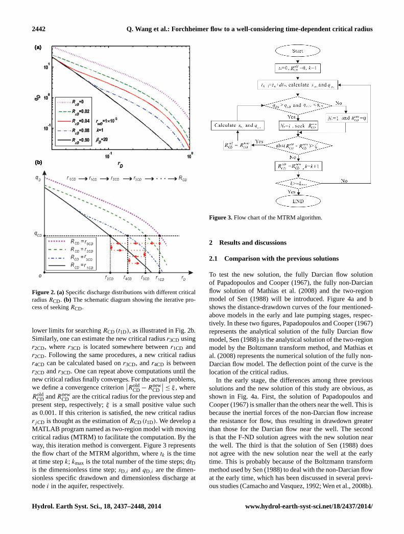
Figure 2a shows the specific discharge distributions withdifferent RCD of 0, 0.02, 0.04, 0.08 and 0.50. The curveof RCD = 0 represents the fully Darcian flow model. Onecan find that the specific discharge decreases with increasingRCD at a givenrD, starting from its maximum atRCD = 0(Darcian flow). This observation is understandable. The in-creasingRCD implies a stronger contribution of the inertialeffect, which also means a larger resistance to flow, thus itleads to a smaller specific discharge. After trying many dif-ferent sets of aquifer parameters, such asβD = 0.002, 0.02,0.2, andRCD = 0.01, 0.03, 0.1, numerical simulation indi-cates that this observation is universally valid. This observa-tion will serve as the basis for the new iteration method toseek the location ofRCD (tD).

Similar to the use ofReC to determine the start of the non-Darcian flow, one can useqCD for the initiation of the non-Darcian flow, whereqCD is the dimensionless critical specificdischarge defined in Table 1. We denoterjCD as the newlycomputed critical radius at thej th step of the new iterationmethod, wherej = 1,2,3. . .. Since the aquifer system is ini-tially hydrostatic, the initial critical radiusr0CD is set to 0.For a given dimensionless timet1D, the detailed proceduresof the iteration method for searchingRCD (t1D) will be in-troduced as follows. First, the specific discharge distributionin the aquifer can be calculated using Eqs. (25)–(33) withRCD (t1D) = r0CD, as shown in Fig. 2b. Based on the com-puted specific discharge distribution, one can find the newcritical radiusr1CD according to a given constantqCD. Sec-ond, the new specific discharge distribution can be similarlycalculated using Eqs. (25)–(33) with RCD (t1D) = r1CD, andthe new critical radiusr2CD can be obtained according toqCD. It is notable thatr1CD andr2CD serve as the upper and



(a)

(b)

Figure 2. (a)Specific discharge distributions with different criticalradiusRCD. (b) The schematic diagram showing the iterative pro-cess of seekingRCD.

lower limits for searchingRCD (t1D), as illustrated in Fig. 2b.Similarly, one can estimate the new critical radiusr3CD usingr2CD, wherer3CD is located somewhere betweenr1CD andr2CD. Following the same procedures, a new critical radiusr4CD can be calculated based onr3CD, andr4CD is betweenr2CD andr3CD. One can repeat above computations until thenew critical radius finally converges. For the actual problems,we define a convergence criterion

∣∣RoldCD − Rnew

CD

∣∣ ≤ ξ , whereRold

CD andRnewCD are the critical radius for the previous step and

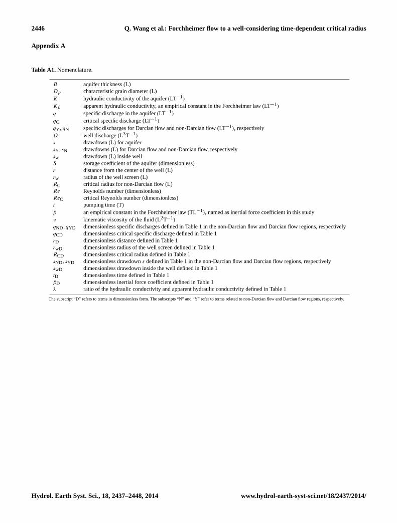
present step, respectively;ξ is a small positive value suchas 0.001. If this criterion is satisfied, the new critical radiusrjCD is thought as the estimation ofRCD (t1D). We develop aMATLAB program named as two-region model with movingcritical radius (MTRM) to facilitate the computation. By theway, this iteration method is convergent. Figure 3 representsthe flow chart of the MTRM algorithm, wheretk is the timeat time stepk; kmax is the total number of the time steps; dtDis the dimensionless time step;sD,i andqD,i are the dimen-sionless specific drawdown and dimensionless discharge atnodei in the aquifer, respectively.

Figure 3. Flow chart of the MTRM algorithm.

2 Results and discussions

2.1 Comparison with the previous solutions

To test the new solution, the fully Darcian flow solutionof Papadopoulos and Cooper (1967), the fully non-Darcianflow solution of Mathias et al. (2008) and the two-regionmodel of Sen (1988) will be introduced. Figure 4a and bshows the distance-drawdown curves of the four mentioned-above models in the early and late pumping stages, respec-tively. In these two figures, Papadopoulos and Cooper (1967)represents the analytical solution of the fully Darcian flowmodel, Sen (1988) is the analytical solution of the two-regionmodel by the Boltzmann transform method, and Mathias etal. (2008) represents the numerical solution of the fully non-Darcian flow model. The deflection point of the curve is thelocation of the critical radius.

In the early stage, the differences among three previoussolutions and the new solution of this study are obvious, asshown in Fig. 4a. First, the solution of Papadopoulos andCooper (1967) is smaller than the others near the well. This isbecause the inertial forces of the non-Darcian flow increasethe resistance for flow, thus resulting in drawdown greaterthan those for the Darcian flow near the well. The secondis that the F-ND solution agrees with the new solution nearthe well. The third is that the solution of Sen (1988) doesnot agree with the new solution near the well at the earlytime. This is probably because of the Boltzmann transformmethod used by Sen (1988) to deal with the non-Darcian flowat the early time, which has been discussed in several previ-ous studies (Camacho and Vasquez, 1992; Wen et al., 2008b).



(a)

(b)

Figure 4. (a) Comparison of the distance drawdowns by the fullyDarcian flow model (Papadopoulos and Cooper, 1967), the fullynon-Darcian flow model (Mathias et al., 2008), the two-region flowmodel (Sen, 1988), and the new model in early pumping stage.(b)Comparison of the distance drawdowns by the fully Darcian flowmodel (Papadopoulos and Cooper, 1967), the fully non-Darcianflow model (Mathias et al., 2008), the two-region flow model (Sen,1988), and the new model in late pumping stage.

The fourth is that there is a deflection point on the new so-lution, leading to discontinuity of the drawdown slope. Thisobservation may be reasonable, as also reported by Mout-sopoulos et al. (2009), who named it non-uniform hydraulicbehavior.

In the late pumping stage, the transient flow approachesthe quasi steady state, and the specific discharge distributionis invariant with time according to Eqs. (3)–(4) or Eqs. (14)–(15), regardless of the Darcian flow or non-Darcian flow. Un-der the quasi steady-state flow condition, the critical radiusobtained by this new solution becomes a constant which isthe same as the one used by previous two-region models suchas Sen (1988) and Wen et al. (2009). Therefore, the new so-lution agrees very well with that of Sen (1988) at late time

Figure 5. Time-dependent critical radius (RCD) for different valuesof the inertial force coefficientβD.

(see Fig. 4b). Another fact that can be seen in Fig. 4b is thatthe new solution agrees with the solution of Papadopoulosand Cooper (1967) in the Darcian flow region.

2.2 Effect of the inertial force coefficient to the criticalradius

The inertial force coefficient (βD) is of primary concern forthe non-Darcian flow described by the Forchheimer equa-tion, and the values ofβD are chosen as 0.001, 0.01, and 0.1.Figure 5 shows the critical radius (RCD) changes with timefor different dimensionless inertial force coefficients. Severalobservations can be seen. First,RCD increases with time un-til the flow approaching the quasi steady-state condition. Inthe early pumping stage, the specific discharge is very largenear the well and decreases quickly with the distance fromthe well, soRCD is very small. With time, the cone of de-pression will expand along the radial direction and the slopeof the cone of depression becomes flatter, soRCD becomesgreater. Second, a largerβD would reduce the rate of changeRCD versus time, thus result in longer time to approach itsasymptotic value, and consequently leads to a smallerRCDat a specific time in the transient state (see Fig. 5). This isbecause a largerβD implies a stronger inertial force, whichincreases the resistance of flow. The third interesting obser-vation is that the asymptotic value ofRCD is the same fordifferentβD. This can be explained using Eq. (2). Based onthe definition of the dimensionless parameters defined in Ta-ble 1, Eq. (2) becomes

qCD = 1/RCD. (34)

Therefore, the value ofRCD does not depend onβD underthe quasi state state flow condition, while it only reciprocallydepends on the critical specific discharge.



Figure 6. Time-dependent critical radius (RCD) for different valuesof the critical specific discharge.

2.3 Effect of the critical specific discharge to the criticalradius

The criterion to judge the initiation of the non-Darcian flowis an important factor of concern. Up to now, there is stillconsiderable debate on what value ofReC to use for the startof non-Darcian low. The recommended values ofReC rangefrom 0.1 to 100 for porous media flow (Bear, 1972; Schei-degger, 1974; Zeng and Grigg, 2006). To check the influenceof ReC on RCD during the transient flow, the values ofqCDare chosen as 100, 50 and 10 considering the direct relation-ship of qCD andRCD in Eq. (2). The other parameters areβD =0.01, andrwD = 1× 10−4.

Figure 6 shows the effect ofqCD onRCD. It is obvious thatthe asymptotic value ofRCD is equal to 1/qCD, as reflectedin Eq. (34). Another interesting observation is thatRCD de-creases with increasingqCD, and it takes shorter time forRCDto approach its asymptotic value.

2.4 Type curves in the non-Darcian flow region andDarcian flow region

Type curves are a series of curves that reveal the functionalrelationship between the well functions (or drawdown) andthe dimensionless time factors (Sen, 1988; Wen et al., 2011).Type curve is one of the common approaches to identify theaquifer parameters or to predict the drawdown (Sen, 1988;Wen et al., 2011). Sen (1988) presented different type curvesin the Darcian flow region and non-Darcian flow region basedon a two-region model. In that model (Sen, 1988),RCD wasa fixed value which only depends on the rate of pumping butindependent of time. In this study,RCD changes with time,and the type curves might be different from the ones gener-ated by Sen (1988). To investigate the behaviors of the typecurves of the new solution, the two observation locations will

Figure 7. Time-drawdown atrD = 0.005 for different inertial forcecoefficients in a log–log scale.

be chosen,rD = 0.005 and 0.02. According to Eq. (34), themaximum ofRCD is 0.001 at the quasi steady state, so theflow at rD = 0.005 will experience both Darcian flow (at theearly time) and non-Darcian flow (at late time), while theflow at rD = 0.02 is always Darcian.

Figure 7 shows the time drawdown atrD = 0.005 for dif-ferent dimensionless inertial force coefficients in the log–logscale. Two interesting observations can be seen from this fig-ure. The first observation is that there is a deflection point inthe curve ofβD = 0.1 or 1, that becomes larger in time withincreasingβD. This is because a largerβD implies a strongerinertial effect, which leads to a larger drawdown and longertime to approach the quasi steady-state condition. This obser-vation is not found in the F-ND model (Wen et al., 2011) andin the two-region model (Sen, 1988). The second observationis that the drawdown in the quasi steady state increases withincreasingβD, and the reason for this has been explained inprevious studies (Wen et al., 2011).

Figure 8 represents the time drawdown atrD = 0.02 in thelog–log scale. One notable point is that flow atrD = 0.02 isalways Darcian, so there is no deflection point in the typecurves. The differences among the curves with differentβDare obvious at the beginning, and then they approach thesame value at the quasi steady state.

3 Summary and conclusions

In this study, a new two-region flow model considering thetime-dependent critical radius (RCD) is established to in-vestigate the groundwater flow into a pumping well, and anew iteration method is proposed to estimateRCD, basedon the finite-difference method. Results show that this iter-ation method is convergence although it has not been ana-lytical verified using rigorous mathematic model. In the non-



Figure 8. Time-drawdown atrD = 0.02 for different inertial forcecoefficients in a log–log scale.

Darcian flow region, the flow is governed by the Forchheimerequation, and the start of the non-Darcian flow is determinedby the critical specific discharge, which is calculated by thecritical Reynolds number. The new solution is compared withprevious solutions, such as the fully Darcian flow model,the two-region model with a constant critical radius, and thefully non-Darcian flow model. The impacts of the dimension-less inertial force coefficient (βD) and dimensionless criticalspecific discharge (qCD) on the critical radius and flow fieldhave been analyzed. Several findings can be drawn from thisstudy:

1. In the early stage, the new solution agrees with thefully non-Darcian flow solution near the well; differswith the fully Darcian flow model of Papadopoulos andCooper (1967) and the two-region model of Sen (1988).

2. In the quasi steady flow stage, the new solution agreeswith the solution of Sen (1988) very well. It agrees verywell with the solution of the fully Darcian flow model(Papadopulos and Cooper, 1967) in the Darcian flow re-gion.

3. RCD increases with time until reaching the quasi steady-state flow, and the asymptotic value ofRCD only de-pends onqCD. A larger βD would reduce the rate ofchange ofRCD with time, and result in a smallerRCDat a specific time during the transient flow state.

4. There is a deflection point in the type curve when theobservation well location is within the non-Darcian flowregion in the quasi steady state whenβD ≥ 0.1, andthe time associated with this deflection point becomeslarger with a largerβD.



Appendix A

Table A1. Nomenclature.

B aquifer thickness (L)Dp characteristic grain diameter (L)K hydraulic conductivity of the aquifer (LT−1)

Kβ apparent hydraulic conductivity, an empirical constant in the Forchheimer law (LT−1)

q specific discharge in the aquifer (LT−1)

qC critical specific discharge (LT−1)

qY , qN specific discharges for Darcian flow and non-Darcian flow (LT−1), respectivelyQ well discharge (L3T−1)

s drawdown (L) for aquifersY , sN drawdowns (L) for Darcian flow and non-Darcian flow, respectivelysw drawdown (L) inside wellS storage coefficient of the aquifer (dimensionless)r distance from the center of the well (L)rw radius of the well screen (L)RC critical radius for non-Darcian flow (L)Re Reynolds number (dimensionless)ReC critical Reynolds number (dimensionless)t pumping time (T)β an empirical constant in the Forchheimer law (TL−1), named as inertial force coefficient in this studyν kinematic viscosity of the fluid (L2T−1)

qND,qYD dimensionless specific discharges defined in Table 1 in the non-Darcian flow and Darcian flow regions, respectivelyqCD dimensionless critical specific discharge defined in Table 1rD dimensionless distance defined in Table 1rwD dimensionless radius of the well screen defined in Table 1RCD dimensionless critical radius defined in Table 1sND, sYD dimensionless drawdowns defined in Table 1 in the non-Darcian flow and Darcian flow regions, respectivelyswD dimensionless drawdown inside the well defined in Table 1tD dimensionless time defined in Table 1βD dimensionless inertial force coefficient defined in Table 1λ ratio of the hydraulic conductivity and apparent hydraulic conductivity defined in Table 1

The subscript “D” refers to terms in dimensionless form. The subscripts “N” and “Y” refer to terms related to non-Darcian flow and Darcian flow regions, respectively.



Acknowledgements.This research was partially supported byProgram of the National Basic Research Program of China(973) (no. 2011CB710600, 2011CB710602), National NaturalScience Foundation of China (no. 41172281, 41372253), thescholarship to Quanrong Wang from China Scholarship Council,Field Demonstration of Integrated Monitoring Program of Landand Resources in Middle Yangtze River Jianghan-Dongtin Plain(1212011120084), and Study on Groundwater Resources and En-vironmental Problems in Middle Yangtze River Jianghan-DongtinPlain (no. 1212011121142). We thank two anonymous reviewersfor the critical and constructive comments that help us improve thismanuscript.

Edited by: S. Attinger

References

Ahmad, N.: Evaluation of groundwater resources in the upper mid-dle part of Chaj-Doak area, Pakistan, PhD, Istanbul TechnicalUniv., Turkey, 1998.

Basak, P.: Non-penetrating well in a semi-infinite medium withnonlinear flow, J. Hydrol., 33, 375–382, doi:10.1016/0022-1694(77)90047-6, 1977.

Basak, P.: Analytical solutions for two-regime well flow problems,J. Hydrol., 38, 147–159, 1978.

Bear, J.: Dynamics of fluids in porous media, Elsevier, New York,1972.

Birpinar, M. and Sen, Z.: Forchheimer groundwater flow lawtype curves for leaky aquifers, J. Hydrol. Eng., 9, 51–59,doi:10.1061/(ASCE)1084-0699(2004)9:1(51), 2004.

Bordier, C. and Zimmer, D.: Drainage equations and non-Darcianmodelling in coarse porous media or geosynthetic materials,J. Hydrol., 228, 174–187, doi:10.1016/s0022-1694(00)00151-7,2000.

Camacho, R. G. and Vasquez, M.: Analytical solution incorporat-ing nonlinear radial flow in confined aquifers – comment, WaterResour. Res., 28, 3337–3338, doi:10.1029/92wr01646, 1992.

Chen, Z. X., Lyons, S. L., and Qin, G.: Derivation of the Forch-heimer law via homogenization, Transport in Porous Media, 44,325–335, doi:10.1023/a:1010749114251, 2001.

Dudgeon, C. R., Huyakorn, P. S., and Swan, W. H. C.: Hydraulics offlow near wells in unconsolidated sediments, Field studies, TheUniversity of New South Wales, Australia, 1972a.

Dudgeon, C. R., Huyakorn, P. S., and Swan, W. H. C.: Hydraulicsof flow near wells in unconsolidated sediments, Theoretical andexperimental studies, The University of New South Wales, Aus-tralia, 1972b.

Dullien, F. A. L. and Azzam, M. I. S.: Flow rate pressure gradientmeasurements in periodically nonuniform capillary tubes, AicheJ., 19, 222–229, doi:10.1002/aic.690190204, 1973.

Engelund, F.: On the laminar and turbulent flows of ground waterthrough homogeneous sand, Tech. Univ. Denmark, Copenhagen,Denmark, 1953.

Ergun, S.: Fluid flow through packed columns, Chem. Eng. Prog.,48, 89–94, 1952.

Forchheimer, P. H.: Wasserbewegung durch boden, Zeitsch-rift desVereines Deutscher Ingenieure, 49, 1736–1749, 1901.

George, G. H. and Hansen, D.: Conversion between quadratic andpower law for non-Darcy Flow, J. Hydraul. Eng.-ASCE, 118,792–797, doi:10.1061/(asce)0733-9429(1992)118:5(792), 1992.

Giorgi, T.: Derivation of the Forchheimer law via matched asymp-totic expansions, Transport in Porous Media, 29, 191–206,doi:10.1023/a:1006533931383, 1997.

Hassanizadeh, S. M. and Gray, W. G.: High-velocity flow in porous-media, Transport in Porous Media, 2, 521–531, 1987.

Huyakorn, P. and Dudgeon, C. R.: Investigation of 2-regime wellflow, J. Hydraul. Division-ASCE, 102, 1149–1165, 1976.

Irmay, S.: On the theoretical derivations of Darcy and Forchheimerformulas – discussion – reply, J. Geophys. Res., 64, 486–487,doi:10.1029/JZ064i004p00486, 1959.

Izbash, S. V.: O filtracii V Kropnozernstom Materiale, Leningrad,USSR, 1931 (in Russian).

Liu, H. H., Li, L. C., and Birkholzer, J.: Unsaturated propertiesfor non-Darcian water flow in clay, J. Hydrol., 430, 173–178,doi:10.1016/j.jhydrol.2012.02.017, 2012.

Louwyck, A., Vandenbohede, A., and Lebbe, L.: Numeri-cal analysis of step-drawdown tests: Parameter iden-tification and uncertainty, J. Hydrol., 380, 165–179,doi:10.1016/j.jhydrol.2009.10.034, 2010.

Mackie, C. D.: Determination of Nonlinear formation losses inpumping wells, International Conference on Groundwater andMan, 5–9 December, 1983.

Mathias, S. A. and Todman, L. C.: Step-drawdown tests andthe Forchheimer equation, Water Resour. Res., 46, W07514,doi:10.1029/2009wr008635, 2010.

Mathias, S. A., Butler, A. P., and Zhan, H. B.: Approx-imate solutions for Forchheimer flow to a well, J. Hy-draul. Eng.-ASCE, 134, 1318–1325, doi:10.1061/(asce)0733-9429(2008)134:9(1318), 2008.

Mishra, P. K., Vessilinov, V., and Gupta, H.: On simulation and anal-ysis of variable-rate pumping tests, Ground Water, 51, 469–473,doi:10.1111/j.1745-6584.2012.00961.x, 2012.

Moutsopoulos, K. N., Papaspyros, I. N. E., and Tsihrintzis,V. A.: Experimental investigation of inertial flow pro-cesses in porous media, J. Hydrol., 374, 242–254,doi:10.1016/j.jhydrol.2009.06.015, 2009.

Papadopulos, I. S. and Cooper, H. H.: Drawdown in awell of large diameter, Water Resour. Res., 3, 241–244,doi:10.1029/WR003i001p00241, 1967.

Quinn, P. M., Parker, B. L., and Cherry, J. A.: Valida-tion of non-Darcian flow effects in slug tests conductedin fractured rock boreholes, J. Hydrol., 486, 505–518,doi:10.1016/j.jhydrol.2013.02.024, 2013.

Scheidegger, A. E.: The physics of flow through porous media, Uni-versity of Toronto Press, Toronto, 1974.

Scheidegger, A. E.: The physics of flow through porous media, Uni-versity of Toronto Press, 152–170, 1974.

Sen, Z.: Type curves for two-region well flow, J. Hydraul. Eng., 114,1461–1484, doi:10.1029/WR024i004p00601, 1988.

Sen, Z.: Nonlinear radial flow in confined aquifers towardlarge-diameter wells, Water Resour. Res., 26, 1103–1109,doi:10.1029/WR026i005p01103, 1990.

Sen, Z.: Non-Darcian groundwater flow in leaky aquifers, Hy-drol. Sci. J.-Journal Des Sciences Hydrologiques, 45, 595–606,doi:10.1080/02626660009492360, 2000.


http://dx.doi.org/10.1016/0022-1694(77)90047-6

http://dx.doi.org/10.1016/0022-1694(77)90047-6

http://dx.doi.org/10.1061/(ASCE)1084-0699(2004)9:1(51)

http://dx.doi.org/10.1016/s0022-1694(00)00151-7

http://dx.doi.org/10.1029/92wr01646

http://dx.doi.org/10.1023/a:1010749114251

http://dx.doi.org/10.1002/aic.690190204

http://dx.doi.org/10.1061/(asce)0733-9429(1992)118:5(792)

http://dx.doi.org/10.1023/a:1006533931383

http://dx.doi.org/10.1029/JZ064i004p00486

http://dx.doi.org/10.1016/j.jhydrol.2012.02.017


http://dx.doi.org/10.1029/2009wr008635



http://dx.doi.org/10.1111/j.1745-6584.2012.00961.x


http://dx.doi.org/10.1029/WR003i001p00241




http://dx.doi.org/10.1080/02626660009492360


Sidiropoulou, M. G., Moutsopoulos, K. N., and Tsihrintzis, V. A.:Determination of Forchheimer equation coefficients a and b, Hy-drol. Process., 21, 534–554, doi:10.1002/hyp.6264, 2007.

Soni, J. P., Islam, N., and Basak, P.: A experimental evaluationof non-Darcian flow in porous media, J. Hydrol., 38, 231–241,doi:10.1016/0022-1694(78)90070-7, 1978.

van Tonder, G. J., Botha, J. F., and van Bosch, J.: A generalisedsolution for step-drawdown tests including flow dimension andelasticity, Water S.A, 27, 345–354, 2001.

Ward, J. C.: Turbulent flow in porous media, J. Hydraul. Division,American Society of Civil Engineers, 90, 1–12, 1964.

Wen, Z., Huang, G. H., and Zhan, H. B.: An analytical so-lution for non-Darcian flow in a confined aquifer usingthe power law function, Adv. Water Resour., 31, 44–55,doi:10.1016/j.advwatres.2007.06.002, 2008a.

Wen, Z., Huang, G. H., Zhan, H. B., and Li, J.: Two-region non-Darcian flow toward a well in a confined aquifer, Adv. Wa-ter Resour., 31, 818–827, doi:10.1016/j.advwatres.2008.01.014,2008b.

Wen, Z., Huang, G. H., and Zhan, H. B.: A numerical solu-tion for non-Darcian flow to a well in a confined aquiferusing the power law function, J. Hydrol., 364, 99–106,doi:10.1016/j.jhydrol.2008.10.009, 2009.

Wen, Z., Huang, G. H., and Zhan, H. B.: Non-Darcian flow to a wellin a leaky aquifer using the Forchheimer equation, Hydrogeol. J.,19, 563–572, doi:10.1007/s10040-011-0709-2, 2011.

Whitaker, S.: The Forchheimer equation: A theoreticaldevelopment, Transport in Porous Media, 25, 27–61,doi:10.1007/bf00141261, 1996.

Yeh, H.-D. and Chang, Y.-C.: Recent advances in model-ing of well hydraulics, Adv. Water Resour., 51, 27–51,doi:10.1016/j.advwatres.2012.03.006, 2013.

Zeng, Z. W. and Grigg, R.: A criterion for non-Darcy flowin porous media, Transport in Porous Media, 63, 57–69,doi:10.1007/s11242-005-2720-3, 2006.


http://dx.doi.org/10.1002/hyp.6264

http://dx.doi.org/10.1016/0022-1694(78)90070-7

http://dx.doi.org/10.1016/j.advwatres.2007.06.002



http://dx.doi.org/10.1007/s10040-011-0709-2

http://dx.doi.org/10.1007/bf00141261


http://dx.doi.org/10.1007/s11242-005-2720-3

forchheimer ﬂow to a well-considering time-dependent

Documents