M I N I S T R Y OF A V I A T I O N

M. No. 3414

A E R O N A U T I C A L R E S E A R C H C O U N C I L

R E P O R T S A N D M E M O R A N D A

Forces on Aerofoils with both Incidence Forward Speed Varying

B y D . G . RANDALL

and

L O N D O N : H E R M A J E S T Y ' S S T A T I O N E R Y O F F I C E

I965

PRICE 13s. 6d. NET

Forces on and

COMMUNICATED

Aerofoils with both Incidence Forward Speed Varying

By D. G. RANDALL

BY THE DEPUTY CONTROLLER AIRCRAFT (RESEARCH AND DEVELOPMENT),

MINISTRY OF AVIATION

Reports and Memoranda No. 34±4 *

May, i964

Summary.

Determination of the inviscid, incompressible flow due to a thin, two-dimensional aerofoil moving with varying incidence and forward speed requires the solution of an integral equation. This report examines the case of harmonic variation of both incidence and forward speed (same frequency, different amplitude and phase). A solution is obtained in which the first terms neglected are of order (v log v) 2, where v is the reduced frequency.

Section

1.

2.

LIST OF C O N T E N T S

Introduction

Two-Dimensional, Unsteady, Inviscid, Incompressible Flow past an Aerofoil

2.1 Flow past a general aerofoil

2.2 Flow past a particular aerofoil

3. Approximate Form of the Integral Equation

4. Solution of the Approximate Integral Equation

4.1 A preliminary result

4.2 The approximate solution

5. Results and Discussion

Symbols

References

Table 1--Coefficients for determining lift and pitching moment

Illustration--Fig. 1. Quasi-steady and corrected lift for a representative aerofoil

Detachable Abstract Cards

* Replaces R.A.E. Tech. Note No. Structures 357--A.R.C. 26 190.

1. Introduction. The determination of the aerodynamic forces acting on a helicopter rotor is a most complicated

problem, and at the present time approximate solutions only can be obtained. A common procedure is to use a 'quasi-steady' theory: at each instant of time the problem is solved by determining the forces produced by a steady flow past the configuration with the current incidence and forward speed. Tl~is clearly results in a substantial simplification, since one of the independent variables,

the time, becomes merely a parameter. The purpose of this report is to obtain an estimate of the error incurred by the use of a quasi-

steady theory. A problem bearing some similarity to the determination of the flow field about a helicopter rotor is solved by two methods; one is a quasi-steady theory, the other is a more accurate theory. It is hoped that the comparison may help to answer the question whether a quasi-steady

theory can adequately predict the aerodynamic forces acting on a helicopter rotor. The problem considered is the determination of the inviscid, incompressible flow due to an

infinitesimally thin, two-dimensional aerofoil that is moving forward with variable speed and oscillating in pitch at the same time. This has some connection with the motion of a helicopter blade: the forward speed of the helicopter combined with the rotatory motion of the blades means that each blade moves normal to its leading edge with variable speed; the incidence of each blade also varies. The assumption of incompressible flow and the restriction to a two-dimensional aerofoil

are easily justified: the forward speed of a helicopter and the speed of rotation of the blades are normally not high enough for compressibility effects to be important; and the aspect ratio of a

helicopter blade is normally large enough for two-dimensional aerofoil theory to be applicable.

As usual, it is assumed that somebody else will investigate the effects of viscosity. The procedure adopted is as follows. Section 2 treats the problem of an arbitrary aerofoil moving

in a straight line w i t h arbitrarily varying forward speed and changing its shape in an arbitrary manner; the problem is reduced to the solution of an integral equation. The analysis is based on that given in Chapter 5 of the book by Robinson and Laurmannl; the reader who has read the chapter may feel that the number of symbols has been reduced; he will be right. At the end of Section 2 the formulas obtained are applied to a flat-plate aerofoil. U, the speed, is assumed to be

given by U = Uo(1 + Y cos ~ot) ; (1)

U 0 corresponds to the linear speed of rotation of a cross-section of a helicopter blade and T U o to the forward speed of the helicopter. ~, the instantaneous incidence, is assumed to be given by

= %[1 + a cos (cot+ e)]. (2)

U0, "i¢, co, s0, a and e are constants, co being the circular frequency; t is the time. Sections 3 and 4 are concerned with the solution of the integral equation derived in Section 2.

In Section 3 an.approximate form of the integral equation is obtained by expanding it in powers

of v, the reduced frequency; u is given by

coC C

V - - U 0 - - ; '

because ~o is equal to Uo/r; here, c is the chord of the aerofoil and r its distance from the axis of rotation. Terms of order unity, . log . , a n d . are retained; terms of order (. log .)2 and higher- order terms are neglected. The approximate integral equation is solved to the same order of accuracy

2

in Section 4. All this obviously introduces another assumption, that v is small compared with unity. For a typical blade the chord is about 15 inches, and the length at least 12 feet; hence, the flow about a blade near its tip corresponds to the flow about the aerofoil satisfying equations (1) and (2) with c equal to 15 inches, and r equal to 12 feet. It follows that

v - 0 . 1 ;

the assumption that v < 1 is, therefore, justified. A representative value for the forward speed (TU0) of the helicopter is 250 feet per second and for the tip speed (U0) 500 feet per second, so that

T = ½ at the tip. Throughout the report it is assumed that T < 1; from equation (1) it is seen that, if T > 1, the value of U is periodically negative, so that the aerofoil periodically moves back into its wake.

In Section 5 it is shown that, not surprisingly, the 'quasi-steady' solution can be obtained by retaining the terms of order unity and neglecting the terms of order v log v and v as well as all

higher-order terms. Section 5 also contains the most important formulas derived in Sections 2, 3

and 4, and a discussion of the results obtained by using these formulas. The reader who wishes to forgo the analysis of Sections 2, 3 and 4 can turn to Section 5 now.

2. Two-Dimensional, Unsteady, Inviscid, Incompressible Flow past an Aerofoil.

2.1. Flow past a General Aerofoil.

Let X and Y be rectangular Cartesian coordinates fixed in space, and let T be time; the origin of these quantities is of no importance. Suppose that the aerofoil is moving along the X axis in the negative direction with speed U(T). The aerofoil is infinitesimally thin, so that, if the local incidence at any point is sufficiently small, boundary conditions on the aerofoil may be satisfied on the section of the X axis momentarily lying between the normal projections on to this axis of the leading and trailing edges. Let the X coordinate of the mid-point of this section be Xm(T), so that

2 ~ ( T ) = - U(T) ; (3)

a dot denotes differentiation with respect to time. Let the density of the fluid be p, the local pressure be p, and the pressure at infinity be Poo. Let the length of the aerofoil chord be c.

Suppose that the conditions (Ref. 1, page 10) for the existence of a velocity potential, ~b, are satisfied; then the components of velocity in the X and Y directions are respectively ~x and ~F, and 6 satisfies Laplace's equation,

4xx + = 0 . (4)

Bernoulli's equation (Ref. 1, page 15) states that at any instant of time

P + + + - (5) 7 2L\ x] aY!.j J r p

The assumptions made about the geometry of the aerofoil allow squares of the velocity components to be neglected in comparison with the velocity components; hence, equation (5) may be approxi- mated by

04 P-p + = T " (6)

(91640) A2

The acceleration potential, g2, is now introduced, where

0 ¢ . (7) ~ - T T '

from equation (4) it satisfies

fL-:x + ~ y r = 0. (8)

From equations (6) and (7), f~ is zero at infinity. The pressure is continuous everywhere except

across the aerofoil, and so the same must hold for f2, from equations (6) and (7); ¢, of course, is

discontinuous across the wake as well, which is why the use of f~ is preferred. Let x and y be rectangular Cartesian coordinates moving with the aerofoil and having their origin

at the point X = Xm(T), Y = 0; let the x axis have the same direction as the X axis. When the space coordinates are x and y, let t denote the time; there is then no doubt about what is being

kept constant during partial differentiations. Hence,

x = X - X ~ ( T ) , (9a)

y = y , (9b)

t = T. (9c) From equation (3), it follows that

~ _ a (10a) ~x ~X'

a (lOb) Oy ~Y'

u( ~ ~ (lOc) -~ = - T) ~--X + a--~.

From equations (8), (10a) and (10b), f~ satisfies

f~x~ + f~vy = 0 ; hence

= ~ ¢(z, t) ,

where ~b is a complex function of z, and

Z=X-l-iy.

In the x, y coordinate system the aerofoil lies between the points ( - c/2, 0) and (c/2, 0); this part of the x axis may be mapped on to the unit circle by the transformation

{) (11, z = ~ ~ + .

Past experience (Ref. 1, page 125) suggests the following form for the function ~b:

¢ = i - a0(t) i - ~ + Z

From the antisymmetry of the problem,

a ( y ) = - ~ ( - y ) .

4

The aerofoil is the only part of the x axis where f2 is discontinuous; therefore, ~2 must be zero along the rest of the x axis and, hence, along the part of the real axis of ~ lying outside the unit circle. It follows that ¢ is a function whose real part is zero along the real axis of ~; hence, the a~(n/> 0)'in equation (12) are all real.

Let the equation of the aerofoil be

y = F(x, t). (13)

The boundary condition is that the velocity component normal to the aerofoil should be zero. The component of velocity in the x direction is U + ex, which is approximately U, and the com- ponent of velocity in the y direction is es ; so the boundary condition is approximately

04) OF OF ~y ~,=o = U ~ + ~ . (14)

On the unit circle, which corresponds to the aerofoil, write

= e i~, (15a) so that, from equation (11),

c x = ~ cos/~. (15b)

The right-hand side of equation (14) can now be expanded as bo/2 + Y, b~ cos n/z, where the b~ n = l

are known functions of t; the boundary condition on the aerofoil becomes

v=o 2 + ~=1 • b~ cos n/~. (16)

From equation (7),

fT f ¢(X, Y, T) = f~ dT~ = N ¢(zi, T~)dT~; (17) - -~9 - -cO

and, from equation (9) here, T 1 is the variable of integration

Zl

the lower limit of the integral can be

= x - X m ( T ~ ) + iV; (18)

replaced by any value of the time early enough for f~ to be zero at the point X, Y, From equations (17) and (18),

O Y~C/' = - J f ~ o~ ~b'(zt' T t )dTl '

where ¢'(z, T) has been written for 3~/3z. From equations (18) and (3),

dz~ = - 2 ~ ( T~)dT 1 = U( T~)dTI ;

(19)

here, T t is to be regarded as a function of zl, given by equation (18); and z is given by

z = x - X ~ ( T ) + i V .

hence, equation (19) becomes

~¢ - J ¢'(~, T~) U(T3; (20) ~Y ~o

On the aerofoil equations (16), (10b) and (20) give

f ' z T d Z l _ b o J -~ ¢ ( ~, 1) U(T~) 2 n=~X b~ cos g/,,, (21)

where - c/2 <~ x <~ c/2. In the integral X is kept constant; x is given by equation (9a), and T 1 (or, in an obvious notation, tl) is given in terms of z 1 by

"gl = X - X m ( T 0 = X - X m ( t l ) , (22)

from equations (18) and (9c). Differentiation of equation (21) with respect to T gives

J ¢ ' ( x , T ) = J ¢ ' ( x , t ) = bo ® ~ ( t ~o ) 2 X b n c o s n t * - U ~ x \ , . , + E bnc°sn t* / , n=l n=l

from equations (10a), (10c) and (9c). Now, from equations (11) and (12),

(23)

¢'(~, t) - a~/a~

hence, on the aerofoil,

From equation (15b),

i a0 oo g/an 1 - i (t + 1 / ~ + 5 * ~T~¥)J

¢'(~, t) -

~. a0£i/z co ~1 4i k(e#'+ 1) 2 + n=* y' g/a~e-iW

2 [ ~0 co 1 c sin ff 2(cos~+ 1) + n=12 na~(cos g//~-isin g/if) .

2 Ox c sin ff a/~

(24)

(25)

(26)

on the aerofoil. From equations (23), (25) and (26),

oo - - ~, na n sin n/, . . . . c sin ff n=l

b0 o~ 2U oo 2 E bn cos g/~ E

n=l C sin/z n=l g/b n sin nff ;

it follows that

c b c bn_l + 4n ~+1 -- Uba (n > 1). (27) an = 4g/

The flow field is completely determined once ¢ is known, and the only unknown quantity in the expression for ¢ given by equation (12) is %. Only the differentiated form of equation (21) has so far been used; substitution of ¢ ' ( z l , I'i) into equation (21) provides the desired relation for a o . From equations (24) and (27),

¢'(z, T) = ¢'(z, t) c ( ~ - 1 ) (~$-1)~ ~ 1 bn_l - ~b~+l + gg/b~

i ~ 4ao~ 2 ( ~ - 1 ) t 4~+1)~

i f 4a0~ 2 (~2-1) t 4~+1)2

- - + (bo+~bd - i E 7 ( ~ - l ) ~ - q

- - + ¢o+ ~bx) - i v ~ + ~ f ~ ~ .

When X and Y are held constant,

d ~ dT 1 0 0 1 dz~ ~z~ + dz~ 3 T 1 ~Zl + U( T 0 ~ T~

from equation (18); in the integral in equation (21), therefore, ~b'(Zl, T1) is given by

i { 4a°~1~ 1) c(~1+ 1) ~ . } ~ZZl ~° bn ,o_ ~'(zl, T 0 - (~1~- - + (bo+ ~lbz) - iU ~ 1 ~1 ~ '

where [1 is defined by

z l = 7, ~1 + • ( 2 8 )

Hence,

f x S(T1)dz 1 [ f x (~12-1)1 [c(~1+ 1) 2/4a°~12 (bo+ ~161)} ~ dzI ~=c° ~ 1 s - ~ ¢'(z~, r l ) - ~ ~ + ,:C= •

From equation (21),

f z 1 / 4ao~1 e (b o+ ~1bl)} dzl b° (29) -oo (g2_ 1) [c(g~+ 1) ~ U(T 0 - 2

The path of integration may be taken as the part of the x axis from - co to x; but x lies in the range - c/2 <<. x <~ c/2, so that the path includes the point x = - c/2; the integral becomes singular there, since, from equation (11), the point x = - c/2 corresponds to ~ = - 1; hence, the path of integration must be indented at the point x = - c/2.

In terms of ~1 equation (29) becomes

f~o~{ 4% 1 (bo+~lbl)} d~ 1 2b o c(~1+1)~ ~ V ( r l ) - ~ '

from equations (28) and (15a); the path of integration runs from - co to - 1 along the real axis of ~1, is indented at ~1 = - 1, and then runs from ~1 = - 1 to ~1 = eie around the unit circle. The last equation may be written

(de 1 / 4a°( T0 4ao( T)/ 2bo -._®(~+1)~ tcU(TO cU(T)J g~ c

(d~, (bo + ~1bl) d~ 4ao(T) (d~' 1 + ~ "0-~ ~d U(TO ~ 7U~(T) .o_~ (~+ 1)~ d~.

(30)

But

~ f ( i l+ 1)~ d~l = - ~ (de+ 1 ~ - ~ ~ + i s i n 1 ,-oo 2 cos ~ 2 '

2 hence, equation (30) becomes

f d ~ 1 /¢__ao(T 0 4%(T)/ 2%(T) 2b o fd~ (bo+ ~bl ) d~ - + 9 ~ ~ .

(~1+ 1) ~ [cU(T 0 cU(r)J d~l cU(T) c . , -~ 1 U(TO

This equation has to be satisfied for one value only of t~, since the differentiated form is known to be true.; when t~ = ~ it becomes

( -~ 1 [4a0(T 0 4ao(T)/ 2a0(T) 2b o i "-1 (b o+ ~lbx) d~ - + . ( 3 1 )

,J--m (~1+1) 2 [cU(TI) ~"~(r)) d~l £U(T) C J --co ~12 U(T1)

From equations (28) and (22),

7, + = x - X m ( ;

at the chosen instant of time, T,/* = ~r, and the last equation becomes

(32)

£ - X - Xm(T), (33)

2

from equations (15b) and (9a); subtraction of equation (33) from equation (32) gives a relation

between ~1 and T 1 with T as a parameter,

c (1 + ~t)~ _ X ~ ( T ) - X~(T~). (34) 4 ~

Provided that a o and U have a Taylor expansion about T 1 = T, it follows that the integrand in the integral on the left-hand side of equation (31) is not singular at ~1 = - 1, so that the path of integration may be taken as the part of the real axis of ~ from - oo to - 1.

Equations (6) and (7) give

P - P o o = - pf~;

hence, the loading at a point on the aerofoil is p ( t ~ , - ~ ) , where D.. and t~ z are respectively the values of ~ on the upper and lower surfaces of the aerofoil; from equations (12) and (15a),

P(~u-f2~) = p (ao tan/z oo ) + 2 ~g a~sinn/z .

The lift on the aerofoil is L, where

L = p J-el2

= ~ p c a o t a n ~ + 2 ?g a~sinn~c s i n ~ d ~ = al), 0 n = l

from equation (15b); the lift coefficient is CL, where

L 7r(a o + al) C~ = 1 = " U ~

P cU2

The moment about the leading edge is M, where

1 ) ci~ 1 + c d x (a -a,>dx + cL

M = p d - e t ~ 2 = p J - e l 2

= p a o t a n ~ + 2 ~ a~sinn/~ 4- 0 n = l

1 sin/z cos 1 ~ dv~ + ~ cL

~pc ~ - - - ( a o + 2 a 1 + a~ ) ;

(35)

the monlent coefficient is C~, where

M Cm - 1

~Z pc~U2

7r(a o + 2a 1 + a~) 4U 2

(36)

2.2. Flow Past a Particular Aerofoil.

Now consider the aerofoil def ined in Section 1. From equation (1),

U ( T ) = U 0 ( l + Y c o s c o r ).

If the mid-point of the aerofoil is at the origin of the (X, Y) coordinates when equations (3), (37) and (9c),

Xm( T ) = - U o T + - sin co T = - U o t + - s i n c o t . co CO

(37)

T = 0, then, from

(38)

From equations (13) and (2), if the aerofoil is assumed to be pitching about the leading edge,

(1) F ( x , t ) = - % { 1 + a c o s ( c o t + e ) } x + ~ c ;

hence, from equation (37),

3 F 3 F ( 1 ) u ~ + ?~ = - ~oUo(1 + - r cos cot) {1 + a cos (cot+ ~)} + %aco sin (cot+ e) x + ~ c

= - ~0 u0(1 + ~ cos cot) {1 + ~ cos (cot + ~)} - - y - sin (cot + ~) +

+ %acox sin. (cot + e),

so that, from equations (14), (16) and (15b)

I acco l bo = - 2% u0(1 + ' r cos cot) {1 + a c o s (cot + ~)} - - U s in (cot + e) , (39)

a°ccoa sin (cot + e), (40) b l = 2

b n = 0 (n > 1). (41)

From equation (39),

bo = 2%Uoco IT sin wt (1 + a cos (o~t+ e)} + a(1 + Y cos cot) sin (cot+ e) +

+ ~- cos (cot + e , (42)

where v is the reduced frequency, cco/Uo; from equation (40),

1 UocoV~ cos (cot+e); (43) bl = 2 ~o

from equation (41),

b~ = 0 (n > 1). (44)

From equations (27), (37) and (39) to (44)inclusive,

1 %Uo2v IT sin a)t {1 + a cos (oat+ e)} + a(1 + Y cos oat) sin (cot+ e) + a 1 = - - ~

a v ] 1% Uo2va(1 + T cos oat) sin (oat + e) + -~. cos (oat + ~) -

1 a o Uo2v IT sin oat (1 + a cos ((at + e)} +

2

+ 2a(1 +)7 cos oat) sin (oat+ e) + ~- cos (oat+ e) , (45)

0~0 C2oa2~ ~0 No 2vza a2 = - 16 cos(cot+e) = l ~ C O S ( o a t + e ) , (46)

a~ = 0 (n > 2) .

To obtain a o equation (31) must be solved. It is convenient to make the following substitutions:

= - UoT/c, (47a)

01 = - - U o T 1 / c , (47b)

Ao(O) = ao(T) Uo%~o(1 + X cos oa T ) ' (47c)

= - ~1. (47d)

From equations (31), (37), (39), (42), (43) and (47),

f¢o _ Ado)} Ao(O) d~/ 1 {Ao(01)

1 ( 7 - 1) ~ 2

= - ( I + Y cos v0){1 + a cos (v0-e)} + ~- sin ( v 0 - e ) -

{[ 1 ( o o v Tsinv01{1 + a cos @01- e)} + a(l + T cos uO1) sin @O 1 - e ) - ~ c o s ( v O 1-e) -

3 2% 2

av 2 [ d~ l . -- 8'r]-~ COS ('1"01--6) J (1+~1 ~ COS V01)'

here, from equations (34), (38) and (47),

(48)

"r 1 ( '71-1)~ (01- 0) + - (sin v61- sin v0) -

v 4 ~71 (49)

10

3. Approximate Form of the Integral Equation.

Equation (48) may be writ ten in the form

Ao(O) = 2(1 + 1 ° cos .0){1 + a cos (vO- e)} + av sin (uO- e) +

+ v ff° [T sin vOl{l + acos(vOl-e)} 1 (1 + Y cos v01)

l d~/1 + a sin (vO 1 - e)/

7112 J

4 1 + (1 + T cos v01) f oo d711

+ 2 1 {A°(Ol) -- A°(0)} i711-- 1) 2. (50)

First, it is shown that the second integral is O(log v). Clearly,

f o~ 2 c o s (1.,0 1 - e)dT] 1 2 f ~ d711 - O(1) ; 1 711 "---~ ~ - - ~ - S - ~ 0 ~ 1 ) ( (1--~ff--~ 1 7112

so it suffices to show that

Write

From equation (49),

f ~ ~ cos (~01- ~)d711 O(log V).

1 711 (1 + ~ cos vOl)

Q1 = (01- 0) + -~ (sin v01-s in vO). V

(51)

(52)

It follows that

1 (71t- 1) 2 Q I "

4 7]z

711 = (1+2Q1) + 2(Q~+ Q12)v~ ; (53)

the positive sign of the square root is required, since, as 01 -+ oo, QI -+ oo and 711->°o. equations (52) and (53),

d711 dQ1 (1 + T cos vO1)dO 1 711 (QI+ Q12) 1/2 ( 9 1 + QP)~/~

From

Therefore, the equation to be verified, equation (51), may be writ ten

j"~ = O(log v). (54) COS 0,ol 6)dO 1 i

o (Q1 + 912)1/~

It is convenient to split the range of integration into two parts by writing

cos ( 01- )d01 to+2-, cos ( 01-e) 01 cos ( 01-e)d01 o ( 9 1 + Q12) ~/~ = / ~o ( 9 1 + 9 7 ) ~ + ) (55) J 0+2~'/v ( Q1 JF 912) 1/2 '

the only significance in choosing 0 + 2rr/u as the intermediate stage is that it makes the analysis simpler; the essential points are that the integrand in the first integral is singular at the lower limit

11

(Q1 = 0 when 01 = 0) but not at the upper one, whereas in the second integral only the upper limit requires care. From equations (52) and (53),

2~r 2rr o ~ = o + - - , Q 1 - , (56a)

/" /"

0 ~ = 0 + - - - ~ = 1 + + 2 + 4 ~ I/~ v /'~ ] = ~A ;

the last equation defines ~7~. Consider the second integral on the right-hand side of equation (55). From equation (52),

(56b)

hence,

0 - Y (sin/'0 t - sin/'0) (1 1 ) I 1 + 1 I = - /" 91

QI( 91 + Q12) 1/2

0 _ .,-T (s in/ '01 - s i n vO) /"

01Q1 +

+ 1 (Q1 + Q12)1/2 [( Q1 + Q1 ~)1/~ + Q1]'

f co COS (/ '0 1 -- e)dO 1 ~,cz cos ( / ' 0 - e)dO 1

0+2;v/v ( Q I + Q12) 1/2 = Jo+27r/v ° l +

® [O-T(sin/'Ol-sin/'O)lcos(/'Ol-e)-

+ dO 1 - o+ ~,~1. Ol Q 1

Co° cos (/'0~- e)d0~ (57)

J 0+~./~ (9~ + 97)1/2 [(Q1 + Q~)1/2 + Q1]"

The first of the integrals on the right-hand side can be written in terms of tabulated functions, as follows:

o +2=//'01 = - c o s e C i ( 2 = + v O ) + s i n e -S i (2~r+v0) ; (58)

here, Ci and Si are respectively the cosine and sine integrals (Ref. 2, page 3), defined by

and

it is known that ~

f co COS vq 1 c i (8) = - ~ s--T- ~ '

sin 81 Si (8) = J ] o ~ de,

7"I" s i (oo) = ~.

Since 2 Ci (27r+/'0) and Si (2~r+ vO) are both O(1), it follows from equation (58) that

f ~ cos ( vO 1 - e)dO~ O(1).

O+2~rfv O1 (59)

12

For the second of the integrals, equation (52) gives

f; + 2~/v

= f;+2~/.

o - r (sin . o l - sin ",o)] cos ( . o l - ~)

OlQ1 dO1

o - r (sin ",01 - sin .o)] cos ( . o l - e) P dO1

< o + _ _ _ - ,

0+2~I. 01 (01 _ 0 -

For the third of the integrals, equations (52) and (56a) give

- 0 ( 1 ) . (60)

f o~ cos ( . 0 1 - ¢)d01 O+2nlv ( Q1 "~ Q12) 1/2 [( Q1 + Q12) 1/2 "{- Qd

= f ~ cos (',01- ~)dQ1 2./v (1 +r cos ",01) (QI + Qlz) 1/2 [(QI+ Q12) 11~ + Q1]

1 f~o dQ1 _ ", - o(~) . (61) < 2(I -~°~ 2./. Q1 ~ 4~(1 - Y )

From equations (57), (59), (60) and (61), it follows that

f f c°s (vOl-e)dOl = O(1) (62) +2.I. (Q1 + Q?)1/2

Now consider the first integral on the right-hand side of equation (55). From equations (52) and (56a),

fo+2~,, cos (<-~)~ol c ~" cos ( , < - ~ ) d Q 1 o ~ Q 7 ~ 1 ~ 5 ~ = /~o ( l + r cos ~00 (QI+ QW( ~

cos (~01- ~) ]~I. = 2 sinh-1Ql1/2 (1 + y c-~ ~0~_] ° +

f2~,. F sin (vOl-e) T sin 1."01 COS (',01--£)] sinh_l Qlll~d01 + 2,, ~o L(1 -}-~' COS ltO1) 2 -- (1 -]-Y COS 1-'01)a

sinh -1 Qll/2 dQ1 < 0 - - ~ ) sinh-1 + 2", (1 --T) 2 + ( ~ y ) 3 oo

- ( l - T ) sinh-1 + 2v ( l - T ) ~ + (1 x

x (1+29 , ) - -~(Ql+Q12)V~]o

] - (1-Y~) sinh-1 + ( l - T ) a 2 (47r+ v) -

= O(log v). (63)

13

From equations (55), (62) and (63), it follows that equation (54) is correct; hence, equation (51) has been proved. Therefore, equation (50) may be writ ten

Ao(O ) = 2(1 + T cos vO) {I + a cos (vO- e)} + av sin (vO- e) +

1 (1 + T cos vOi) + a sin (vO i - e)l d3-!l +

r/is

f co

+ 2 {ao(O,) - ao(O)} d71 i (71- 1) s

- - + O(v s log v)

= 2 ( l + Y cos vO) {1 + a cos (vO-e)} + a sin (vO-e) +

+ ~ iT sin ~0 {1 + ~ cos (~0- ¢)}

where

A = a c o s ( v 0 i - e ) +

(1 + T cos vO) + a sin (vO- e)l +

+ ~ fo~ Ad01 foo d71 - - - - + 2 {A°(01) - A°(0)} (71 1) s + O(vs log v), (64)

0 71 1

Y cos vO 1 [1 + a cos (vO 1 - e) - aT sin I"01 sin @01- e)]

T s sin s vO i [1 + a cos (vO i - e)]

(1 + T cos v0i)s +

(1 + T cos vOi) +

Clearly,

Y [cos vO 1 + a cos (2vO 1 - e)] T s sin s vO 1 [1 + a cos ( v O 1 - e)] (65) = a c ° s ( v O i - e ) + ( l + T cos vOi) + ( I + T cos vOi) s

Y( 1 + a) ys(1 + a) IAI < " + (1-TW + ( l - Y ) 2 " (66)

It is now shown that the last but one integral in equation (64) is O(log v). The range of the integral is split up into two parts by writing

f* A dOl f°+~'l" A dO~ f ~ AdO 1 = + (67) o ~71 o o 71 o+2~rlv 71

First, consider the second integral. From equations (52) and (53),

0 - _T (sin vO 1 - s i n vO)

- - - ~11 = - - 4 0 1 Q 1 + 2 ( Q I + Q l S ) % - ( 2 Q 1 - 1 ) 4Q171

0 - T__ (sin vO i - sin vO) (8 G - 1)

4Q17 i [2 (Qi+ Qi~) ~/2 + ( 2 Q , - 1)] ; = _ +

401Q1

f ~ A dO~ _ A d O 1 a f~ o+2.1~ 7 i o + s . l ~ 71~ - + 4 o+s~,l~

A [ O - T (sin vO l - s i n

01Q1 dO1 -

co

-- 4 dJ'e+2,r/v A(8 Q1- 1)d01 91,1 [ 2 ( 9 ~ G q ~ T (2 91 - 1)]" (68)

hence,

+ (4;1

14

For the second of the integrals on the right-hand side, equations (52) and (66) give

A [ O - Y (sin vOl - s in

E 7) f d01 o+2~I. 01 0 I - 0 -

\ V /

T(1 +a) Y_~(I+ a)] (2~r+ vO) 0(I). (69) = a + ( 1 _ _ r ~ + (1- - r )2_ j log 2(=_~c~ -

For the third of these integrals, equations (52), (53), (56a) and (66) give

f ~ A(8 Q1- 1)dO~

o+~.t. Qlnl [2(Q1+ Q12)~/~ + (2Q1-1)] f ~ A(8 Q1-1 )dQ1 J 0+2./. (1 +Y cos vOOQ 1 [2(91+ Q12) 1/~ + (2Q1+ 1)] [2(Q1+ Q12) 1¢~ + (2Q1-1)]

8 [ r(l+a) r~(l+a)] f~ dQ1 < (l~=r-~ a + ( l - Y ) ~ (1-Y)2_I 2./, 4Ql (4Ql -1)

2 [ Y(l+a) T2(l+a) -] 8~- = O(v). (70) - (1 - Y ) a + (1 - ~ ) - + (1 _y)2 ] log (S~r- v---~

From equations (68), (69) and (70)

f~ A dO~ _ l f ~ A dO~ 0+2~/~ nl 4 o+2./, 01 + O(1). (71)

Equation (65) may be written as

( Y - a cos e) ( l -Y2) ( Y - a cos e) a ( 1 - Y 2 ) s ines invO~ A = 2acos(u0 l - e ) + - -

r(1 + Y cos v00 Y(1 + Y cos vO0 ~ (1 + T cos v01)~ N o w ,

( [ 1 (l-Y2)_ .] Tsin vO 1 (1 + r cos vO1) - (1 + r cos v01)~] do1 = v(1 +Y cos uO 0 ' t ] L-

and f sin vO 1 dO 1 1

(1 + r cos v01) 2 vY(1 +1~ COS V01)" From the last three equations and equation (58),

f a cos e)sin vO 1 oo AdO1 2alCi(2=+~0)[ + 2 a Si(2rr+v0) + L ~01(l+'fcos~00 0+2~r/. 0 1 < - - - -

a(1 - T z) s ine "] ~ I 1 fo~ F(Y-a cos e) sin vO 1 a(1 - Y~) sine -] doll

I (T+a) a(1 -Y~)

< 2alCi(2~+.O)[ +2a _ - Si(2~,+.O) +(l_T)(2~+~@+T(l_T)(2~,+.e)+

1 F(v+ a) a(1--r') l aol + -~ L ~ - Y ) + r(1-~;)JJo+~./. ol ~

2 = 2alCi (2=+uo) I + 2a - si (2~-+vo) + (2~+~,0~) L(1-~) +

= o ( 1 ) .

15

From this equation and equation (71) it follows that

f ~ - O(1) (72) d dO 1

o+27d~ ~1

Now consider the first integral on the right-hand side of equation (67). From equations (52), (53) and (56@

fi+2~l~ A d 0 1 = (~t~ A{(I + 2Q1) - 2(QI + QI~)I/~}dQ1

~< (l+~;cos ~01) Q~ + QI"= ~ (G+Qd) '2(I+2Q3 + 2 sinh-lQl~/2 + o I

+ .,o dO, ( l + Y c o s v 0 , ) ] Q I + Q , 2 _ (Q,+Q,Z) ' /2 ( I+2Q,)+

1 sinh-lQ1 v2 } dO~ (73) + ~

From equation (66), ]A[ = O(1); (74)

from equations (65) and (66),

d A V01) = v I T sin vO 1 _ a sin (vO 1 - e) dO t (1 + r cos (1 _~.~o COS P012) (1 -~P COS V01)

Y{sin vO~ + 2a sin (2vOw- e)} "f~ sin v01{cos v01 + a cos (2v01- e)} - (1 +-F cos vO~) 2 + (1 + 2 ° cos v01) 3 +

~1 "2 [2 sin vO~ cos v01{1 + a cos (v01- e)} - a sin 2 vO~ sin (u01- e)] + +

(1 + T cos v01) 8

2-F a sin ~ v01{1 + a cos (vO~ - e)} + (1 + T cos vO~) ~

r t rIl+a) c(1+2a/ < v L(1 __f)z [ a + (1 - -Y~ + ~ ) ~ ) + ( 1 - ~ ) + (1 - ¥ ) ~ + (1 -- l ' ) ~ +

Now,

-F2(2 + 3a) 2~£3(1+ a)~ + (1- 'Y) 3 + ~ - ~ ) ~ / = O(v). (75)

d 1 1 dQ~-i [Q~ + Q12 - 2 (Q1 + Q12)1f2( 1 + 2Q1) + ~ sinh-1 Q11I~] =

= (1 + 2 Q 1 ) - 2 ( 9 1 + 9 7 ) '~

= [(1 +2Q1 ) + .2(Q1 + Q ~)1/2]-1. 1 This is always positive in the range of integration, so the maximum of [Q1 + Q1 z - ~ (Q1 + Q12) ~/~

1 (1 +2Q1 ) + ~ sinh -1 Q1 ~/2] in the range occurs at Q1 = 2~/v. Hence,

1 1 Q1 + Q1 ~ - ~ (QI+ QI~)~/~( 1 +2Q1) + ~ sinh-1 Q1 ~/2

<~ --v + v ~ - - 2 + v~- ] 1 + + ~ sinh -~ = O(log v). (76)

16

From equations (73), (74), (75) and (76),

fo+2~l~ = O(log v). 4 d O t

o ~]1

From this equation and equations (67) and (72),

j .~o A dot _ O(log P) .

o ~1 Hence, equation (64) becomes

Ao(O ) = 2(1 + T cos vO) {1 + a cos (vO- e)} +

I r a i n ~0{1 + a cos ( ~ 0 - ~ ) } 1 +v 2asin(vO-e)+ (1 + Y cos 70) +

+ 2 {Ao(00 - Ao(0)) d~i 1 i~l-- 1) - ~ + O(v2 log v).

This is the required approximate form of the integral equation, equation (48).

(77)

(78)

(79)

4. Solution of the Approximate Integral Equation. 4.1. A Preliminary Result.

The problem considered in this section is the expansion of the integral

f o~ ( l + T cos vO 0 {1 + a cos ( rOt-e)} - ( I + Y cos vO) {1 + a cos (vO-e)} d~/1 t ( ~ t - 1) 2

as a term in v log v plus a term in v plus higher-order terms. It is convenient to write

f ~ (1 + Y cos vO~) {1 + a cos (vO t - e)} - (1 + T cos re) {1 + a cos (uO- e)}

1 ( ~ t - 1) ~

I aT{c°s(2vOl-e) -c°s(2vO-e)} l ~C(cos ~O, - cos ~0) + a{cos ( ~ 0 t - e) - cos ( ~ 0 - e)} + dr/1

J t ( % - 1) 2 aT J(2, ~), = Y J(1, O) + a J(1, e) + ~-

where / '~ cos ( n ~ e l - 8) - cos ( n ~ e - a)

J(n, 3) d r h . J 1 O h - 1) e

After an integration by parts,

J(n, 3) = [ - c°s(nvO1-8)-c°s(nvO=8)]°°-nvf ~sin(nvOt-a)(w 1) J~ o ( % - 1) dot"

From equations (52) and (53),

,im[ co ( 01 ', ,,] E "}1 ~1~o ~ t - 1 : ~1~o - 2 Q1 + ~ 7 4 Q - 1 ~ 7 e-

l -nvsin(nvO t - 8 ) ( l + T c o s v O 0 ~ m ° = o,

= " - 2 1 + 2(Q1 + Q ?) '~

by l 'H6pital 's rule; so equation (81) becomes

f~°sin(nvOt-8) n, f= sin(nvOa-8 ) J(n, 3) = - nv dO 1 o ( ~ = 1 ~ = - 2 o [Ol + ( G + Qd) 'q dot,

. (80)

(81)

(82)

(83)

17

(91640) B

from equation (53)• Split the range of integration into two parts and write

( ~ sin (nvO 1- 8) ~0+~,~t. sin (nvO 1- 8)dO 1 ~ sin (nvO 1- 8)d01 0 [Q1 + (Q1 + Q12) a/2] do1 = ijo [Q1 + ( _01 + Q12)I/s] + ,} O+2~r/. [Q1 + (Q1 + Q1B)a/s] ' J

Consider the second integral on the right-hand side. From equation (52),

271 2 + 2~71 QI+(QI+Q1V/~ =

0 - _T (sin vO 1- sin vO)

hence,

2OxQ1

0 - T__ (sin vO 1- sin vO) 1J

+

= _ + 2OLQ1

( Q1 + Q12) it°" -- Q1 2Q1 [Q1 + (Q1 + Q12) ats]

1 2 [Q1 + (QI+ Q?)>-]= '

f ~ sin (nvO 1- 8)dO 1 1/.~o sin (nvO 1- 8) dO 1 o+~./. [QI + (Q1T QI~) l/s] = 2 Jo+2./. ol

+

1 ~ [0 - T_v (sin v01-sin vO)] sin (nvO 1- 8)d01

f __ _ + 2 o+~,/~ 01Q1

The first of the integrals on the right-hand side of this equation can be written as s

f ~ sin (nv01-8)dOa= cos8[2-S i (2wn+nvO)]+s i r~SCi (2wn+nvO' ; 0+27r/v 01

Si (2wn+nvO) and Ci (2wn+nvO) are both 2 O(1), so that

f oo sin (nvO a - 8) =

dO t O(1). O-k27r/v 01

For the second of these integrals, equation (52) gives

,o~ [ 0 - T-(sinvOl-sinvO)] sin(nvOl-8)dO 1 O

= f [0 - i I]] : 0:-: in vO ) ] s i 2 }n_v01~ 8) d01

01[(01-O)+~(s invOl-s invO) 1

o+2~I. 01 0 1 - O - -

For the third of these integrals, equations (52) and (56a) give

f ~ sin (nvO 1- 8)dO 1

< 4(1-~c~ J~/~ Q? 8~(1 - r ) O(v).

1 [-~o sin (nvO 1- 8)dO 1 2 Jo+2./~ [Q1 + (QI+ Q12)at2] 2"

- O ( 1 ) .

(co sin (nvO I - 8)dQ1 ) ~./. [Q1 + (QI+ Q?)I/-"P (1 +'c cos ~01)

18

(84)

(85)

(86)

(87)

(88)

From equations (85), (86), (87) and (88), it follows that

f ~ sin (nvO l - 3) o+~./~ [Q1 + ( Q I + Q12) 1L~] = do1 = 0(1). (89)

From equations (85), (88), and (52), this integral can be approximated by

[ ~ sin (nvO 1 - 8)d01 1 _(~ sin (nvO 1 - 3) 0+27r/v [Q1 + (Q1 + Q12) 1/2] = ~ --O+27r/v Q1 dO1 + O(v). (90)

Now consider the first integral on the right-hand side of equation (84). From equations (52) and (56a),

~.o+~1. sin (nvO 1 - 3)d01 [.2~/. sin (nY01- ~)dQ1 ! ! oo [Q1 + (Q1 -I- Q12) 1t2] , o (1 +r COS v01) [Q1 + (QI+ Q12) 1/2]

= ( l+Tcosv0x) sinh-1 + + v 2] - -

(o+~,I~ In cos (nvO x - 3) Y sin vO 1 sin (nvO 1 - ~)] - - V

. o [ [ i T g ~ o s ~ ? ~ + (1 + r cos ~01) ~

x [sinh -1 Q1112 + (Q1 + Q12) ~/2 - Q1]dOl • NOW,

sinh-1 + + v ~] v =21°g- -v + ~ + O ( v ) '

and, from equation (52),

[1 LOTf~osVO~) + (1 + r cos ~01) ~

. r [ ~ + O ,

n Y I (1 + 201 ) (Q1 + QI~) 1/2 + g sinh-1 Qi 1/2 + - - + 2-Jo - ( 1 - Y ) ~ + ( ~ -

= O(log v);

1 here, the fact that

be written

(o+~/~ sin (nvO1-3)dO 1 = 1 ( --+18w ) sin (nvO-3) ~o [Q~+(Q1+Ql~)l/2] ~ log v ( l+Ycosv0 )

~o L(1 +37 cos v01) +

1 ( l o g 8 W + l ) s in (nvO-3 ) 2 v (1 + 2" cos vO)

- v ~o dO1 L ( I + Y cos v01) +

N

(91)

+ Q1- (QI+ QI~) 1/"] aQ1

+ Q1 - (QI+ QI~) 1/'-' > 0 for 0 ~< Q1 < co has been used. So equation (91) may

sinh -1 011/°- + O(v log p). (92)

19

Y sin vO 1 sin (nvO 1 - 3)] (1 +Y cos vO1)~ J

From equation (56@

"~o L ( 1 - Y cos ~01)

= rl sin(nvOl-S) Lt(1 + r cos ~01)

Now,

T sin u0, sin (nvO,- 8)] sinh_, Qi>.dO i + (1 + Y cos vOi) 2 • sin (nvO- 3) I "qo+~,,f~ ( i ;Y~OS vO-)J sinh-1 Ql1/2]0 - -

_ 1 [ ~ " r sin ( ~ 0 1 : a ) sin (n,07 8) ] dQ1 2~o L(~+r~os~01) ( l + r c o s ~ 0 ) J (91+97)>- 1 [z~,~ F sin (~nv-01: S) sin (rive-- 3)] dQi 2~o k(i+roos~Ol) (i +-r cos ~0)J (g1+g~)~/~

f 2.t, [ sin (~tvO 1 - ~) o L(~7-~s 7071) < F[ sin (TtPO 1 - ~)

L[(1 + T cos ~,01)

f°o+z"t~Fncos(nvOl-3) TsinvOlsin(nvOl-8) 1, + " L ( I + Y cos 1201) -~" (1 "]-Y COS P01) g X

x [log Qt + 2 log 2 - 2 sinh -1 Q1 ~/2] dO 1

F recos( o -a) v sin vO_l_sin_(nVOl-- 8)] = " o.o L(1 + T cos ~,o~) + (1 + T cos ~,01) ~ ] ×

dQi p01) x [log Q1 + 2 log 2 - 2 sinh -i Qi ~I~ (1 + g cos

from equations (52) and (56@ Hence,

fi ,. r sin ( , ,<- si_n (m,0-3).] 11 1 dQ1 L(i-F+Y~gd~) (1 + T cos vO)_] (01 (Q1-I--QI~)"~_I

I " " IY < " ( 1 z r ) ~ + ( - - : ~ ) ~ ~o

= v (1 - r ) ~ + ( ~ - Q~ log 91

- 2Qi log 2] 27rlv

I0 = O(v log v);

here, the equations

f o+~t~ sin (nvO i - 8)dO i o Q1 + ( Q1 + Q?)lq

sin (nvO- 8) ~ 1 1 ] ( g l + -Q12) 112J (1 + r c o s ~0)J [~ dQ1

sin (nvO- 3) / q 2.I~ (17- Y c~Ts ~0) J {log Q1 + 2 log 2 - 2 sinh -1 Qll/2}J ° +

+ Qi + (1 +2Qi ) sinh-r Q11/" - (Qi+ Q12) z/2 -

(93)

(94)

(95) fact that [2sinh -1Qi 1 / 2 - 1 o g Q i - 2 1 o g 2 ] > 0for0~< Qi < ~ has been used. From (92, (93) and (95),

( 8zr ) s in(nvO-8) l f~ ,~Fs in( .~ ,o~-~ ) ~in ( , , ,O-~) ]dQ~ 1 l o g - - + 1 + L( l+Ycos vO1) ( l + Y c o s vO)[ ~-1 = 2 v (1 + T cos vO) 2 ~o

1 ( l o g ? + 1 ) s i n (nvO- 3) = 2 0 7 - ~ J o ; ;0) +

+ 2 ~o L(1 +Y cos ~,0~) sin (nvO- 3) ] (I+T (i; 7os ;0)j

cos O1)d01 Q1

+ O(v log v)

20

+ O(v log v), (96)

from equations (52) and (56a). From equations (83), (84), (90) and (96),

_ _ _ ( 8~ ) s in(nv0-3) J(n, 8) = nv I o g - - + l

4 v (1 +T cos vO)

nv (°+2"/" F sin_ (nVel-_ 3 ) sin (nvO T 3)_l ( l +.F cos O1)dO, -

4 J0 / ( l+~ 'cos ~01) (l + r cos .0)] Q1

n v

f o~ sin (nvO I - 8) dO1

4 0+2~/, -~)~- + O(v2 log v) = O(v log u),

from equations (89) and (90). Change the variable of integration from 01 to X where

X = v01' Equation (97) then becomes

J(n, 8) n sin (nvO- 8) nv K(n, 8) + O(v 2 log v) - 4 ( I + T cos vO) v log v - -~-

where sin (nv0- a)

K(n, 8 ) = (log 8~r+ 1) + z) + [ sin 8) sin/- 0- 8)] (1+ r cos x)dx

J,0 L(1 + T cos X) (1 +T cos v0)J R

here, from equation (52),

R = vQ~ = ( x - vO) + T(sin x - s i n vO).

From equation (80),

f ~ (1 + r cos ~0~) [1 + a cos ( . 0 1 - e)] - (1 + -r cos ~0) [1 + a cos ( ~ 0 - e)] d71

1

fco + sin ( n x - 3) dX" 2n 4-vO R '

(71- 1) 2

1 I sin vO sin (vO - e) sin (2vO- e) 7] = T¢ , T ( l + T c o s vO) + a ( l + Y c o s vO) + a~° (~-Y~o~7#)-J vlogv -

1 4 [TK(1, 0) + aK(1, e) + aTK(2, e)]v + O(v 2 log v).

(97)

(98)

(99)

(100)

4.2. The Approximate Solution.

It is now shown that the approximate solution of equation (77) is [ T s i n v 0 { l + a c o s @ 0 - e ) ! 1

A o ( O ) = 2 ( l + Y c o s v O ) [ l + a c o s ( v O - e ) ] + 2 a s i n ( v O - e ) + (1 + T cos .0) v +

[~f sin vO + a sin (vO - e) + aT sin (2vO - e)] + v log v -

(1 + T cos vO)

- IrK(l, 0) + aK(1, e) + aTK(2, e)]v + O[(u log v)2]. (101)

Write equation (77) as

Ao(O) - 2(1 +W cos vO)[1 + a cos (vO-e)] -

- u [2a sin (vO-e) + Tsinv0{l(l+Tcosv0)+acos(v0-e)}]_ 2G[Ao(O)] + O(v21ogv)=0,(102)

Where G is an operator.defined by

G[f(O)] = [f(01) - f(O)] d T ~ 1 ( 7 1 - 1) 2 .

21

Clearly G[U(0)] = kG[/(O)], (103)

when k is a constant, and G[f~(O) +fz(0)] = G[f~(O)] + G[f2(O)]. (104)

If Ao(O ) as given by equation (101) is to satisfy equation (102), then, from equations (100), (103) and (104), the following equation must be true:

vTG [ sin vO{1 + cos (vO-e)}] 2auG[sin ( . 0 - e ) ] + (1 + Y cos vO) +

[ { sinvO } [ sin(vO-e) } [sin(2vO-e) t] + v log v YG (1 + Y c ~ s vO) + aG [ ( f T f c ~ T s ;3) + aTG [ ( I + T cos vO)J_.] -

- ~]"G[K(1, 0)] - ~aG[K(1, e)] - ~ a r a [ K ( 2 , ~)] = o[(~ log ~)~].

To prove this it is sufficient to show that

a [s in (vO- e)] = O(v log v), (105)

[sin vO{1 + acos(vO-e)}j = O(v log v), (106) G (1 + Y cos vO)

F sin (nvO- 8) ] o k 0 ~ - Y J o s Y0)j = o(~ log , ) , (107)

and G[K(n, 6)] = O(v log v), (108)

where n is equal to 1 or 2 and 8 is equal to 0 or e. Equat ion (106) can be writ ten

I :in vO + 72 sin (2vO - e) + ~ sin e

G ( I + T cos vO) = O(vlog v);

from equations (103) and (104), the proof of this is dependent only on the proof of equation (107), with n now equal to 0, 1 or 2.

Equation (105) is

j ,~o [sin @01- e) - sin (vO- e)]&?l O(v log v). 1 (~1- 1) ~

NOW,

f ~ [sin (vO~- e) - sin (vO- c)]dy]l

(71-17

= J 1 , ~ + e = O(v logv ) ,

f rom equation (97); this proves equation (105). Equation (107) is

~o [- sin (nv01-8) sin (nvO_--_6) ] d~71 f l k(l+Tcos~,01-) ( l+~;cos~,0)d (~1-1 ) ~

22

- O(v log v).

Split the range of integration into two parts by writing

f o~ sin (nv~- 8) sin (nvO- 8) ] &h (1 +T cos v01) (1 + r cos vO)l 071- 1) 2

= ~v~ r sin (nvO 1- 8) sin (nvO- 8) ] d~l

t Csin( ,01-8) sin_ (uu0_- 3) ] dv:t + j L ( I+Y~s . : ,~ ) (1 + r cos ~,0),_1 @1-1)2'

YA

where ~ is given by equation (56b). Now,

f °° rsin(nv01-8) sin(nvO-3)] dT]l • ,,~ L(I+YG~-;~) (~:kYEosTF)J (V~-1) ~ < - - -

2 v (1 - T ) (TLa- 1) (1 - T ) [2~v + (4w2 + 27rv)~/q

hence, from equations (109) and (56b),

r sin ( . ,01- 8) sin (nu0-- 8)_] d,1 f l L(~7-YGd~V~) (l+Vcos~O)j (.1_1)2

p r : ~ ) sin ( n . 0 - 8) ] d"ql 1 L ( l + Y c o s ~ ' G ) ( l +"C cos v0)J @ 1 - 1 ) 2

- [ 1 [ sin(nv01---8) L @ 1 - 1 ) / ( l + Y cos v01)

(109)

(1 - r ) 3~,~ @1-1)~

o ( ) .

+ o(~)

sin

f[ +2,/~ [n cos(nvOl__8 ) T sin v0] sin (vO~-8)] dO1 + v L(1 +T cos v01) + (1 +T~oos ~-1) ~ _1 (~7~1) + O(v). (110)

From equations (56), the upper limit in the first term vanishes; the argument used to prove equation (82) shows that the lower limit also vanishes. Hence, from equation s (52), (53), (56a) and (110),

, f : [ s in (nvO,-3) sin (nvO-3)] d,1 L(]~-Y~osV~/) (Tr+-Tc~-)/(,~--1)"

= 2 L(1 + r cos .@2 + (1 + r cos ,ol) ~ [(21 + ( G + g?)l/-] + 009

P I < 2 i1-=0 2 + (1--Y)~j-~0 [G + (o1+~ g? ) ' q + o(,)

= 2 ( l - T ) ~ + ~ QlV2 + + - (1 sinh-~ (gl 97)~/°- 110 +o(~)

= O(vlog v); (11i)

this proves equation (107).

23

To prove equation (108) it is sufficient to demonstrate the truth of both

~ I~(2"+~°l)/sin ( n x - 3 ) f* -~0x /(1 +-r cos ~)

_ ~(2"+~°)t sin ( n x - 8 )

and

sin (nvO,- 8) t (1 +Y cos x)dx ~ - + - 1 ~ COS vO1) ) R 1

sin (nvO- 3) t (1 + T cos x)dx-] drh _ O(v log I]),

(1 + T cos ~0)) R ] (~1- 1) 2 (112)

sin (n X - 3) dX sin (n X - 3) d~% - O(v log v) . (~+~o~) -R-~ - (~.~,,o) ( ~ - 1)~ '

(113)

where equations (98), (111), (103) and (104) have been used; here,

and R1 = (X - v01) + Y(sin X- sin vO~),

R = ( X - v O ) + T(sin X-sin uO),

from equation (99). Equations (112) and (113) are proved by splitting the range of integration into two, as before; the expressions are now fairly cumbersome, and it is hoped that the reader will be satisfied with a brief sketch of the procedure; the arguments are very similar to those used before.

Consider equation (112) first. Split the range of the outer integral into two, 1 to %,, and ~7.4 to oe, where %~ is given by equation (56b). The inner integrals are both O(1), and so are less than C,

where C = O(1); hence, the outer integral from ~A to oo is less than C ~ d~71/Oh-1) =, which d VA

is O(v). The outer integral from 1 to ~TA is integrated by parts: 1/031-1) times the inner integral at ~11 equal to ~?A is O(v); 1/(~,-- 1) times the inner integral vanishes as ~, -+ 1, exactly as in the proof of equation (82). The remaining term is v times a double integral. This double integral is less

~ 27r+0 than C dO~/(~ h - 1), where C is O(1); as in the proof of equation (111), this can be shown to

, ) 0

be O(log v). Hence, equation (112) is true. A similar argument holds for equation (113); here, the inner integrals are known to be O(1) from equations (89), (90) and (52). Since equations (112) and (113) are both true, it follows that equation (108) is also true.

All four relations of equations (105) to (108) have now been verified, so that Ao(O ) is indeed given by equation (101), the error being O[(v log v)2].

5. Results and Discussion. From the analysis in the preceding three sections, approximate expressions can be obtained for

Co, the lift coefficient, and C~n, the moment coefficient referred to the leading edge. From equations

(35) and (37),

CL = ~(ao+ al) U02(1 +Y cos cot) 2 ; (114)

from equations (36) and (37)

w(a0 + 2 a l + a2) C,~ = 4Uo2(1 + y cos oot) 2" (115)

24

Here, from equation (45),

a 1 s

, 12 - ~ {T sin cot [1 + a cos (cot + e)] + 2a(1 + T cos cot) sin (cot + e)} + O(v s) ; (116a)

f rom equation (46),

and, from equation (47c),

as = O(vS) • (116b) O~ U o s

a° - (1 + T cos cot)A o. ~Uo s

F rom equations (101) and (47a),

n o = 2(1 + r cos cot) {1 + a cos ( c o t + @ -

- u log ~ {Y sin/ot + a sin (cot+e) + aT sin (2cot+ e)} _ (1 + Y cos cot)

Y sin cot{1 + a cos (cot+ e)} -12 2as in (co t+e )+ (1 + r cos cot)

+ a Y K ( 2 , e)] + 0[(12 log ~2) s]

here, f rom equations'(47a) and (98) (with y written for -X) ,

sin (ncot+ 3) K ( n , 8) = - (log 87r+ 1) (1 + V cos cot) +

f ~t [ sin (ncot+ 3) sin (ny+ 8) ] (1 + T cos y)dy

hot-21r)

where, from equations (99) and (47a),

R = (cot- V) + Y(sin cot- sin Y).

+ YK(1, 0) + aK(1 , e) +

(117a)

(l17b)

f (~JI-2n) d ~

- sin (ny + 8) • • / -¢o - R '

These formulas give C L and C m as terms O(1) plus terms O(v log v) and O(v); terms O[(u log u) 2] and higher-order terms are neglected. When v is put equal to zero, the formulas give the 'quasi- steady' results, C z = 2~rao(1 + a cos (cot+ e)], C m = (rr/2) %[1 + a cos (cot+ e)]; here, from equation (2), %[1 + a cos (cot + e)] is the instantaneous incidence. Consequently, an idea of the error incurred by the use of quasi-steady theory can be obtained by comparing the terms O(u log v) and O(u) in C L and C m with the terms O(1).

Now, the formulas for C L and C m may be written in the following form:

- [1 + a c o s ( c o t + e ) ] + v [ l 1 + 1 2 1 o g v ) + ( m l + r n s logv) a s i n e + 27i'~ 0

+ ( n l + n s log .)a cos e] + O[(v log v) 2] ; (118)

- [1 + ~z cos (cot + e)] + v[(/3 + ls log v) + (ms + ms log v)a sin e +

+ (na+ns log v)a cos e] + O[(v log v)2]. (119)

These follow from equations (114) to (117) inclusive. Table 1 gives values for l l , lS, etc: for each of five values of T(0, 0.2, 0- 4, 0.6, 0.8) the quantities are given for twelve values of cot (0 to llrr/6 at intervals of ~r/6).

25 (91640) C

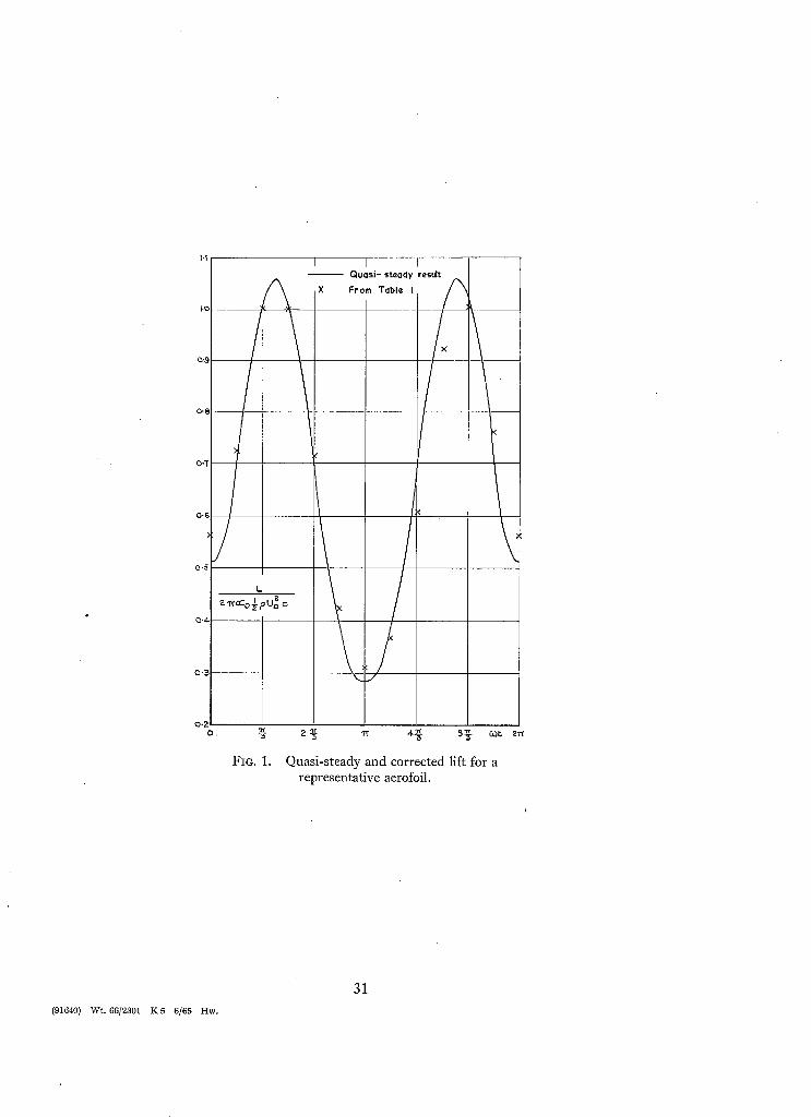
In Fig. 1; L (non-dimensionalised by dividing by 2~rao½pUo2c) is plotted against cot for repre-

sentative values (for a helicopter blade) of -F, a, v and e; these are "I" = 0.6, a = 0.8, v = 0 . 1

e = 7r. The full line is the quasi-steady result,

L 27r%½p Uo2c (I + Y cos ~ot) 2 [1 + a cos (oJt + e)],

the crosses are the values obtained by using Table 1. I t is seen that in this example retention of

terms O(v log v) and O(v) makes little change to the quasi-steady curve.

The special case where a is unity and Y is zero corresponds to constant forward speed and harmonic variation of incidence. Since Y = 0, e may be chosen arbitrarily; i t is taken to be zero. This case is treated in Ref. 1 (page 503), where an exact solution is obtained. For a reduced frequency of 0- 1, the following results are obtained for the non-dimensionalised L.

cot Quasi-steady Present theory Exact theory 1

0 2 1.922 1.916

~r/2 1 1" 056 1" 038

zr 0 0" 078 0" 084

3w/2 1 0" 944 0" 962

2~r 2 1" 922 1" 916

The terms O(v log v) and O(v) produce the differences between the second and third columns; the terms O[(v log v) ~] and higher-order terms produce the differences between the third and fourth

columns.

After the present work had been completed, the author's attention was drawn to two papers by

issacs ~, 4. Isaacs considers the same problem as the one treated in this report. His method is to solve

equation (48) by expanding it as a Fourier series in vO (that is, in oJt). The Fourier coefficients are

complicated functions of Bessel functions; but, in principle, any number of them can be calculated.

Isaacs gives results only for an example where there is constant incidence and harmonic variation of forward speed (see Ref. 3). He truncates the Fourier series at the terms in cos 4cot and sin 4cot,

because the coefficients of these are already small enough to be neglected. It seems likely that the

same will be true for the general case (incidence and forward speed both varying); if so, Isaacs's

method will be more satisfactory than the present one, since it effectively provides the exact solution.

However, it is felt that the present analysis is of sufficient interest to warrant publication.

In Isaacs's example a = 0, Y = 0.4, and v = 0.0848; since a = 0, there is no need to specify e. The following results are obtained for the non-dimensionalised L.

cot Quasi-steady Present theory Issacs's theory a

0 1.96 1. 947 1. 947

7r/2 1 1" 047 1" 039

7r 0" 36 0" 430 0" 427

3zr/2 1 O" 954 O" 963

2~" 1" 96 1" 947 1" 947

The terms O(v log v) and O(v) produce the differences between the second and third columns; the terms O[(v log v) 2] and higher-order terms effectively produce the differences between the third and fourth columns.

26

A

Ao

a

a 8

bs

Ci

CL

Cm

C

F

G

J

K

L

ls , ms, ns

M

P

P ,

0_1 R

Ri

It

Si

T,t

T1, tl

U

uo X

Xm X

Y

Y

z

SYMBOLS

Defined by equation (65)

Defined by equation (47c)

See equation (2)

See equation (12)

Defined after equation (15b)

Cosine integral (see page 3 of Ref. 2)

Lift coefficient

Coefficient of pitching moment about leading edge

Aerofoil chord

y = F(x, t) is aerofoil equation

Operator defined after equation (102)

Defined after equation (80)

Defined by equation (98)

Lift acting on aerofoil

See equations (118) and (119)

Pitching moment about the leading edge

Pressure

Free-stream pressure

Defined by equation (52)

( X - uO) + T(sin X + sin vO)

(X-v01) + T(sin X-s in v01)

Length of blade

Sine integral (see page 3 of Ref. 2)

Time (T when space coordinates are X and Y, t when they are x and y)

Variable of integration

Aerofoil speed

See equation (1)

Coordinate: origin fixed in space and lying on flight path, but otherwise immaterial; direction opposed to that of aerofoil motion

X coordinate of mid-point of aerofoil

Coordinate: origin at X = X m ; direction the same as that of X

Coordinate: origin same as that of X; direction perpendicular to that of X

Coordinate: origin same as that of x; direction perpendicular to that of x

27

S Y M B O L S - - c o n t i n u e d

Z = X + @

z I = X - X.~(tl) + i Y ; on the aerofoil, X - X.~(tl)

Aerofoil incidence

% See equation (2)

y Variable of integration

e See equation (2)

~1 z l = ~ ~1 +

%~ = ( 1 + ~ ) + 2 ( ~ + v~ ]

o = - Uot/~

O~ = - U o t J C

tz ~ = e#'

v Reduced frequency

p Density

T See equation (1)

¢ Velocity potential

X = v01

¢ ~ = ~ ¢ ( z , t)

f~ Acceleration potential

co Circular frequency

No. Author(s)

1 A. Robinson and J. A. Laurmann

2 E. Jahnke and F. Emde . . . .

3 R. Isaacs . . . . . . . .

4 R. Isaacs . . . . . .

R E F E R E N C E S

Title, etc.

Wing theory. C.U.P. 1956.

Tables of functions. Dover Publications. 1945.

Airfoil theory for flows of variable velocity. J. Ae. Sci., Vol. 12, No. 1, p. 113. January, 1945.

Airfoil theory for rotary wing aircraft. J. Ae. Sci., Vol. 13, No. 4, p. 218. April, 1946.

28

T A B L E 1

Coefficients for Determining Lift and Pitching Moment

cot

0 ~-/6 ~-/3 ~-/2

2~'/3 57r/6

"27"

7~'/6 4~/3 3zr/2 5~'/3

1 1 ~ ' / 6

cot

0 ~r/6 ~/3 ~r/2

2~/3 57r/6

qT

7~'/6 4~'/3 3~/2 5~r/3

11~'/6

cot

0 vr/6 7r/3 7r/2

27r/3 57r/6

7T

%v/6 4~-/3 3~-/2 5w/3

117r/6

/7'/1

-0 .59546 -0 .12299 +0.38244 +0.78540 +0.97791 +0.90839 +0.59546 +0.12299 -0 .38244 -0 .78540 -0.97791 -0 .90839

/ /1

-0 .78540 -0.97791 -0 .90839 -0-59546 ~0.12299 +0-38244 +0-78540 +0.97791 +0.90839 +0-59546 +0.12299 -0 .38244

Y = O

12

0 0 0 0 0 0 0

! 0 I

0 0 0 0

m 2

-0 .50000 -0.43301 ~0.25000

0 +0.25000 +0.43301 +0.50000 +0-43301 +0.25000

0 -0 .25000 -0-43301

///2

0 -0 .25000 -0-43301 -0 .50000 -0-43301 -0-25000

0 +0.25000 +0.43301 +0.50000 +0.43301 +0.25000

0 0

0 0 0 0 0 0 0

i 0 0 0

m 3

- 1 - 0 9 5 4 6

-0 .55600 +0-13244 +0.78540 + 1.22791 + 1.34140

! + 1.09546 +0-55600 -0"13244 -0"78540 - 1-27791 - 1 " 3 4 1 4 0

1/13

-0 .78540 - 1.27791 - 1.34140 - 1-09546 -0 .55600 +0.13244 +0-78540 + 1.22791 + 1.34140 i + 1.09546 +0.55600 -0 .13244

T = o . 2

-0 .10833 -0 .07917 -0-03355 +0.02988 +0.11237 +0.19924 +0-24241 +0-19385 +0.07890 +0.03032 -0 .09563 -0-11706

m 1

-0 .49061 -0-05826 +0-38354 +0-76178 +0.99374 +0-99497 +0.73126 +0.23106 --0.36892 --0.82487 --0"97598 --0"83166

/ /1

-0 -65080 -0 .78631 -0 .71605

• -0 .44875 -0 .01389 +0.50185 +0.96671 + 1-23391 + 1-16420 +O-76O64 +O-19991 -0 .30901

0 -0 .03633 =0.07157 -0 . 10000 -0 . 10692 -0 -07314

0 +0.07314 +0.10692 +0.10000 +0-07157 +0-03633

m 2

-0 -41667 - 0 . 3 5 0 9 2 -0 -16529 +0-10000 +0-37037

+0 -56030 +0.62500 +0.56030 +0.37037 +0.10000 -0 .16529 - 0 . 3 5 0 9 2

/'Z 2

0 -0 .24455 -0 . 42944 -0 .50000 -0 .42766 -0 .23903

0 +0.23903 +0-42766 +0-50000 +0-42944 +0.24455

Y = 0 . 4

-0 .10833 -0 .09733 -0 .06933 -0 .02012 +0.05891 +0.16268 +0.24241 +0.23042 +0-13236 +0.01968 -0 .05984 -0 .09890

m 3

--0-90728 --0.41827 +0.18726 +0.81178 + 1-31782 + 1-53679 + 1.35626 +0.77307 --0.04485 --0.77487 -- 1-17226 -- 1-19166

/ /3

-.0.65080 - 1.01514 - 1.12760 -0 .94875 -0 .46829 +0.23114 +0-96671 + 1-50462 + 1-61859 + 1.26064 +0.61144 -0 .08019

-0 .15479 -0 .10704 -0 .04087 +0.05791 +0.22879 +0.53351 +0.83033 +0.68077 +0.24354 -0 .05499 -0-16822 -0-18346

m 1

-0 .40943 -0 .01708 +0.37648 +0-75106 + 1.03939 +1-09597 +0.89936 +0.42924 -0 .33471 -0 .88515 -0 .98233 -0 .76614

/ /1

-0 .54763 -0 .64038 -0 .56536 -0 .31149 +0.15299 +0.73537 + 1.20697 + 1.56939 + 1-51910 +0-94629 +0.25993 -0 .25987

12

0 -0 .05516 -0 .12028 -0 .20000 -0.27063 -0-23409

0 +0.23409 +0.27063 +0.20000 +0.12028 +0.05516

//'/2

-0 .35714 -0 .29402 -0-10417 +0-20000 +0-54688 +0.77956 +0.83333 +0.77956 +0.54688 +0.20000 -0-10417

I -0-29402

II 2

0 -0.23345 -0 .42099 -0 .50000 -0.40595 -0 .17978

0 +0-17978 +0-40595 +0.50000 +0.42099 +0.23345

Y = 0 . 6

-0-15479 -0 .13462 -0-10101 -0 .04209 +0-09347 +0.41646 +0.83033 +0.79782 +0.37886 +0.04501 -0-10808 -0 .15588

m 3

--0.76658 --0.32490 +0.22023 +0"85106 + 1-46908 + 1.81701 + 1.73270 + 1.15027 +0.09497 -0 .78515 - 1.13858 -- 1.07395

///3

-0-54763 -0 .84995 -0 .95628 -0-81149 -0 .32061 +0.45424 + 1.20697 + 1.85052 + 1.99271 + 1.44629 +0"65085 -0 .05031

-0 .17010 -0 .11046 -0 .03325 +0.08168 +0.31415 + 1-06083 +2.57775 +2-08138 +0-57951 -0 .06200 -0 .21487 -0 .21396

m 1

-0 .34603 +0-01058 +0.36290 +0.75120 + 1.16098 + 1.22566 + 1.03224 +0.87485 -0 .28647 -0 .97503 -0 .99016 -0 .70649

/ /1

--0.46864 -0 .52849 -0"44661 --0"18753 +0.42306 + 1.33522 + 1.41378 + 1.91347 +2.02717 + 1.15609 +0.30738 -0"21890

0 - 0 . 0 6 4 9 6 -0 -15373 - 0 . 3 0 0 0 0 - 0 - 5 3 0 2 2 - 0 . 6 5 0 0 0

0 +0-65000 +0.53022 +0.30000 +0.15373 +0.06496

m 2

--0-31250 --0.25247 --0.05917 +0.30000 +0"81633 + 1-22639 + 1-25000 + 1.22639 +0-81633 +0.30000 --0.05917 --0-25247

/ /2

0 - 0 . 2 2 0 7 7 -0 -40996 - 0 . 5 0 0 0 0 - 0 . 3 5 3 4 8 +0.04250

0 - 0 . 0 4 2 5 0 +0.35348 +0.50000 +0.40996 +0-22077

-0 .1 7 0 1 0 "0-14294 --0.11011 --0.06832 +0.04904 +0-73583 +2-57775 +2.40638 +0.84462 ~0.08802 --0~13801 --0.18148

m 3

-0 .65853 -0 .25813 +0.23715 +0.90120 + 1.74772 +2-28955 +2-28224 + 1.93873 +0-30026 -0 -82503 - 1 . 1 1 5 8 9

-0 -97520

/ /3

- 0 . 4 6 8 6 4 -0 .72113 --0.81813 --0.68753 --0.06298 + 1.09626 + 1.41378 +2.15243 +2.51320 + 1-65609 +0-67890 -0 -02626

ll

--0-16827 --0.10168 --0.01730 +0.10051 +0.27305 + 1-32581

+ 11.33460 +7.60139 + 1.31715 --0.02243 --0.23189 --0.22184

m 1

-0 .29584 +0.02930 +0.34694 +0.76109 + 1.45578 + 1.69904 +0.16022 +2.23415 -0 .27757 - 1.11418 - 1.00458 -0 .67511

n 1

-0 .40662 -0 .44096 -0 .35164 -0 .07485 +0-89308 +3-76832 -0 .16515 + 1.28941 +2.78648 + 1.39221 +0.34685 -0 .18919

T = 0 . 8

0 -0 .06979 -0-17674 -0-40000 -0.96225 -2 .11956

0 +2.11956 +0.96225 +0-40O00 +0-17674 +0.06979

m 2

-0 .27778 -0 .22090 -0.02551 +0.40000 +1.25000 +2.46942 +2"50000 +2"46942 + 1.25000 +0"40000 -0"02551 -0 .22090

/ /2

0 -0.20813 -0 .39766 -0 .50000 -0 .24056 + 1.02174

0 - 1.02174 +0.24056 +0.50000 +0.39766 +0.20813

-0-16827 -0-13658 -0 .10566 -0 .09949 -0 .20809 +0-26603

+ 11-33460 +8.66117 + 1.79828 +0.17757 -0 .14352 -0 .18694

m 3

-0 .57362 -0 .20904 +0"24489 +0.96109 +2.28910 +3.63857 +2.66O22 +4-17367 +0.55576 --0.91418 - 1 . 1 0 6 6 2

-0 .89546

n 3

-0 .40662 -0-61886 -0 .70513 -0-57485 +0-41194 +3.87227 -0 .16515 + 1.18547 +3.26760 + 1-89221 +0.70033 -0 .01129

29

(9164o) D

0.3

I.q)

(3.9

0.8

o.'l

0 .6

o.. =

J

Z W~Co½pUo z c

I

X

I I Quas i - steady resdt

From Table I

I.I

\

O.

FIG. 1. Quasi-steady and corrected lift for a representative aerofoiL

(91640) Wt. 66/2301 K 5 6/65 Hw.

31

Publications of the Aeronautical Research Council

A N N U A L T E C H N I C A L R E P O R T S O F T H E A E R O N A U T I C A L R E S E A R C H C O U N C I L ( B O U N D V O L U M E S )

I942 Vol. I. Aero and Hydrodynamics, Aerofoils, Airscrews, Engines. 75s. (post as. 9d.) Vol. II. Noise, Parachutes, Stability and Control, Structures, Vibration, Wind Tunnels. 47s. 6d. (post as. 3d.)

x943 Vol. I. Aerodynamics, Aerofoils, Airscrews. 8os. (post 2s. 6d.) Vol. II. Engines, Flutter, Materials, Parachutes, Performance, Stability and Control, Structures.

9os. (post as. 9d.) x944 Vol. I. Aero and Hydrodynamics, Aerofoils, Aircraft, Airscrews, Controls. 84 s. (post 3s.)

Vol. II. Flutter and Vibration, Materials~ Miscellaneous, Navigation, Parachutes, Performance, Plates and Parlels, Stability, Structures, Test Equipment, ~Vind Tunnels. 84s. (post 3s.)

1945 Vol. I. Aero and Hydrodynamics, Aerofoils. I3os. (post 3s. 6d.) Vol. II. Aircraft, Airscrews, Controls. I3os. (post 3s. 6d.) Vol. I IL Flutter and Vibration, Instruments, Miscellaneous, Parachutes, Plates and Panels, Propulsion.

I3OS. (post 3s. 3d.)" Vol. IV. Stability, Structures, Wind Tunnels, WindTunne l Technique. 13os. (post 3s. 3d.)

1946 Vol. I. Accidents, Aerodynamics, Aerofoils and Hydrofoils. i68s. (post 3s. 9d.) Vol. II. Airscrews, Cabin Cooling, Chemical Hazards, Controls, Flames, Flutter, Helicopters, Instruments and

Instrumentation, Interference, Jets, Miscellaneous, Parachutes. i68s. (post 3s. 3d.) Vol. III. Performance, Propulsion, Seaplanes, Stability, Structures, Wind Tunnels. 168s. (post 3s. 6d.)

1947 Vol. I. Aerodynamics, Aerofoils, Aircraft. 168s. (post 3s. 9d.) Vol. II. Airscrews and Rotors, Controls, Flutter, Materials, Miscellaneous, Parachutes, Propulsion, Seaplanes~

Stability, Structures, Take-off and Landing. I68S. (post 3s. 9d.)

t948 VoL I. Aerodynamics, Aerofoils, Aircraft, Airscrews, Controls, Flutter and Vibration, Helicopters, Instruments, Propulsion, Seaplane, Stability, Structures, Wind Tunnels. r3os. (post 3 s. 3d.)

Vol. II. Aerodynamics, Aerofoils, Aircraft, Airserews, Controls, Flutter and Vibration, Helicopters, Instruments, Propulsion, Seaplane, Stability, Structures, Wind Tunnels. x Ios. (post 3s. 3d.)

Special Volumes Vol. I. Aero and Hydrodynamics, Aerofoils, Controls, Flutter, Kites, Parachutes, Performance, Propulsion,

Stability. ia6s. (post 3s.) Vol. II. Aero and Hydrodynamics, Aerofoils, Airscrews, Controls, Flutter, Materials, Miscellaneous, Parachutes,

Propulsion, Stability, Structures. I47S. (post 3s.) Vol. III. Aero and Hydrodynamics, Aerofoils, Airscrews, Controls, Flutter, Kites, Miscellaneous, Paraehutes¢

Propulsion, Seaplanes, Stability, Structures, Test Equipment. I89S. (post 3s. 9d.)

Reviews of the Aeronautical Research Council 1939-48 3s. (post 6d.) I949-54 5s. (post 5d.)

Index to all Reports and Memoranda published in the Annual Technical Reports I9o9-1947 R. & M. 2600 (out of print)

Indexes to the Reports and Memoranda of the Aeronautical Research Council Between Nos. 2351-2449 R. & M. No. 2450 as. (post 3d.) Between Nos. 2451-2549 Bet~veen Nos. 2551-2649 Between Nos. 265I-a749 Between Nos. 2751-2849 Between Nos. 2851-2949 Between Nos. 295 I-3o49 Between Nos. 3o51-3149

R. & M. No. 2550 2s. 6d. (post 3d.) R. & M. No. 2650 as. 6d. (post 3d.) R. & M. No. 275 ° 2s. 6d. (post 3d.) R. & M. No. 2850 2s. 6d. (post 3d.) R. & M. No. 295 o 3s. (post 3d.) R. & M. No. 3o5 o 3s. 6d. (post 3d.) R. & M. No. 315o 3s. 6d. (post 3d.)

HER MAJESTY'S STATIONERY OFFICE f rom the addresses overleaf

R. & M. No. 3414

© Crown copyright i965

Printed and published by HER MAJESTY'S STATIONERY OFFICE

To be purchased from York House, Kingsway, London w.c.2

423 Oxford Street, London w.x I3 A Castle Street, Edinburgh z

xo 9 St. Mary Street, Cardiff 39 King Street, Manchester 2

50 Fairfax Street, Bristol x 35 Smallbrook, Ringway, Birmingham 5

80 Chichester Street, Belfast x or through any bookseller

Printed in England

R. & M. No. 3414

S.Oo Code No. 23-3414