forage yield and quality estimation by means of uav and

Vol.:(0123456789)

Precision Agriculture (2021) 22:1437–1463https://doi.org/10.1007/s11119-021-09790-2

1 3

Forage yield and quality estimation by means of UAV and hyperspectral imaging

J. Geipel1 · A. K. Bakken1 · M. Jørgensen1 · A. Korsaeth1

Accepted: 20 January 2021 / Published online: 18 March 2021 © The Author(s) 2021

AbstractThis study investigated the potential of in-season airborne hyperspectral imaging for the calibration of robust forage yield and quality estimation models. An unmanned aerial vehi-cle (UAV) and a hyperspectral imager were used to capture canopy reflections of a grass-legume mixture in the range of 450 nm to 800 nm. Measurements were performed over two years at two locations in Southeast and Central Norway. All images were subject to radiometric and geometric corrections before being processed to ortho-images, carrying canopy reflectance information. The data (n = 707) was split in two, using half the data for model calibration and the remaining half for validation. Several powered partial least squares regression (PPLSR) models were fitted to the reflectance data to estimate fresh (FM) and dry matter (DM) yields, as well as crude protein (CP), dry matter digestibil-ity (DMD), neutral detergent fibre (NDF), and indigestible neutral detergent fibre (iNDF) content. Prediction performance of these models was compared with the prediction perfor-mance of simple linear regression (SLR) models, which were based on selected vegetation indices and plant height. The highest prediction accuracies for general models, based on the pooled data, were achieved by means of PPLSR, with relative root-mean-square errors of validation of 14.2% (2550 kg FM ha−1), 15.2% (555 kg DM ha−1), 11.7% (1.32 g CP 100 g−1 DM), 2.4% (1.71 g DMD 100 g−1 DM), 4.8% (2.72 g NDF 100 g−1 DM), and 12.8% (1.32 g iNDF 100 g−1 DM) for the prediction of FM, DM, CP, DMD, NDF, and iNDF content, respectively. None of the tested SLR models achieved acceptable prediction accuracies.

Keywords UAV · Hyperspectral imaging · Multivariate statistics · Forage · Yield · Quality

Introduction

Efficient and precise grassland management and feed planning are key factors to increase the economic profitability of ruminant livestock production. To support farm-ers in their management decisions, regarding timing of harvests, fertilization rates and feed purchase, updated information on the prevailing field situation and harvested forage

* J. Geipel [email protected]

1 Norwegian Institute of Bioeconomy Research, Pb 115, 1431 Ås, Norway

http://orcid.org/0000-0002-7171-9501

http://crossmark.crossref.org/dialog/?doi=10.1007/s11119-021-09790-2&domain=pdf

1438 Precision Agriculture (2021) 22:1437–1463

1 3

is necessary (Schellberg et al. 2008). Particularly in regions with long winters and long periods of indoor feeding, robust estimates on forage yields and quality are valuable. Remote sensing technology offers tools that have the capacity to assist farmers with such information (Weiss et al. 2020).

Many studies have already shown the potential of hyperspectral remote sensing together with multivariate regression techniques for the determination of cereal grain yield and quality (Fu et al. 2014; Kusnierek and Korsaeth 2015; Øvergaard et al. 2013, 2010). Although such technology may be less important for production on grassland farms than on cereal farms (Schellberg and Verbruggen 2014), it has received increasing attention in research on forage management over the last years (Wachendorf et al. 2018).

A number of grassland studies have focused on field spectroscopy, commonly using handheld point spectrometers that are sensitive in a wavelength range of around 350 nm to 2500 nm, featuring a high spectral and radiometric resolution. This technology has been shown useable to predict forage yields and forage quality parameters, e.g. crude protein content or fibre content (Safari et al. 2016; Zhou et al. 2019), within a limited spatial area. For any practical purposes, however, the spectral data acquisition requires more efficient approaches. One option is to use an aircraft as platform for the sensor sys-tem. Several authors have shown that the use of pushbroom hyperspectral instruments mounted on a manned aircraft has a high potential for forage yield and quality predic-tions (e.g. Cho et al. 2007; Pullanagari et al. 2018, 2016). Since this approach requires a fully equipped aircraft and a pilot, it is very costly, and the setup may be a constraint for the flexibility needed in busy periods during the cropping season.

The use of unmanned aerial vehicles (UAVs) represents a cheaper and more flexible alternative. When reviewing remote sensing as a tool to assess key properties of temper-ate grasslands, Wachendorf et al. (2018) stated that UAVs and hyperspectral imaging systems may play a major role in rapid and non-destructive sampling of such informa-tion. So far, published studies on grassland using hyperspectral imaging on a UAV have been carried out with a rather limited number of ground truth samples. To the authors’ knowledge, the most extensive work in this regard has been conducted by Wijesingha et al. (2020), who reported a sample size (n) of 194, focusing exclusively on the pre-diction of forage quality. Moreover, the literature revealed that studies utilizing multi-variate methods for analysing hyperspectral data in grassland studies are scarce. The standard approach is based on the use of simple vegetation indices, comprising only a few variables (i.e. wavebands). There is a risk that by using only a very limited number of bands in the electromagnetic spectrum, valuable information is left out, as shown for wheat yield and quality estimation (Øvergaard et al. 2013, 2010). Capolupo et al. (2015) compared statistical approaches for analysing hyperspectral data from a grassland trial (n = 120) and concluded that a multivariate method (partial least squares regression, PLSR) was superior to the methods based on selected vegetation indices for predicting structural and biochemical features.

In this study, the possibilities of combining UAV-borne hyperspectral imaging technol-ogy with multivariate statistics have been explored in order to design a rapid and robust tool to provide accurate in-season estimates of both grassland (forage) yields and quality. A relatively comprehensive data set (n = 707) was acquired from field trials designed to mimic typical forage production systems. The trials were conducted over two years in two of the major Norwegian agricultural regions, representing both humid continental and mar-itime climate. The study focused on the development of thoroughly validated and general-izable prediction models for forage yields and some of the most important feed parameters. In addition, prediction performance of multivariate models and models based on common

1439Precision Agriculture (2021) 22:1437–1463

1 3

vegetation indices was compared. The study builds upon the initial work of Geipel and Korsaeth (2017), comprising additional data and analyses.

Materials and methods

Experimental sites

Field experiments were conducted at Apelsvoll and Kvithamar, two research stations of the Norwegian Institute of Bioeconomy Research (NIBIO), located in South-East and Central Norway, respectively.

At Apelsvoll (APE; 60.70 ° N, 10.87 ° E; elevation 251 m a.s.l.), the average annual pre-cipitation (1961–1990) is 600 mm, of which 319 mm fall in the growing season (May–Sep-tember), and the average annual air temperature is 3.6 °C (12 °C in the growing season). The soil is an imperfectly drained brown earth with dominantly loam and silty sand tex-tures, developed from moraine till deposits.

At Kvithamar (KVI; 63.49 ° N, 10.87 ° E; elevation 25 m a.s.l.), the average annual pre-cipitation (1961–1990) is 900 mm, of which 416 mm fall in the growing season (May–Sep-tember), and the average annual air temperature is 5.0 °C (11.7 °C in the growing season). The soil is a poorly drained silty clay loam, developed from marine sediments.

Field experiments

At each of the two sites, a mixed sward field trial was established at the end of June 2015. Timothy (Phleum pratense L., cv. Grindstad), meadow fescue (Festuca pratensis, cv. Fure) and red clover (Trifolium pratense L., cv. Lea) were sown with a weight-based seed mix ratio of 77:20:3, respectively, and at a sowing rate of 25 kg ha−1. At sowing, 50 kg N ha−1 was applied as a NPK compound fertilizer. In the middle of August, the sward was cut once to a stubble height of 70 mm.

In 2016, the trials were laid out according to a split-plot design with fertilizer rate as main plot (summing up to 130 kg N ha−1 year−1, 200 kg N ha−1 year−1 or 270 kg N ha−1 year−1) and time of harvest as sub-plot (early or normal first cut). The trial at APE con-sisted of five replicates and a total of 120 plots (6.0 m × 1.5 m), whereas that at KVI con-sisted of six replicates and 144 plots (5.5 m × 1.5 m). Both trial layouts are shown in Fig. 1.

The leys were fertilized in spring (40 kg N ha−1, 80 kg N ha−1 or 120 kg N ha−1), after the first cut (30, 60 or 90 kg N ha−1), and after the second cut (60 kg N ha−1 in all treat-ments). The different fertilizer treatments were not chosen to investigate the effect of the applied N on plant growth but to ensure larger variation in plant matter and quality for a more robust model calibration.

In each of the years 2016 and 2017, a three-cut regime was chosen, which is repre-sentative for silage production practice in these regions. Half of the plots were harvested at early heading of timothy, and the remaining plots one week later, corresponding to approx-imately 90 growing degree days (GDD, base temperature 0 °C; Table 1). The second cut included all plots and was scheduled to be harvested approximately 550 GDD after the later first cut. The third and final cut was harvested around 10 September, but these data were not included in the study, since there is a general practice to harvest as late in the season as possible, thus making it difficult to obtain representative models for the final cut. The two first harvests (first cut), designated ‘early’ and ‘normal’, were both within the


1 3

range of phenological development stages of the plants in which farmers in the regions normally time their harvest. The yield and fibre content will normally increase at a high rate between these two stages, whereas the digestibility will decrease.

Fig. 1 The mixed sward field trial in Kvithamar (a) and Apelsvoll (b) with a typical Norwegian seed mix, laid out according to a split-plot design with five and six replicates and a total of 120 plots and 144 plots in Apelsvoll and Kvithamar, respectively. Fertilizer rate was allocated to main plots, and time of harvest (early or normal first cut) to the sub-plots

Table 1 Harvest dates, growing degree days (GDD, base temperature 0 °C) and precipitation sum for the first two cuts

a Accumulated in the period from the day of estimated growth start according to Grovfôrmodellen (Nord-skog et al. 2018) until harvest of the first cutb Accumulated in the period from 1. cut (normal) until harvest of the second cut

Year Location 1. cut (early) 1. cut (normal) 2. cut

Date GDDa Pre-cipitationa [mm]

Date GDDa Pre-cipitationa [mm]

Date GDDb Precipi-tationb [mm]

2016 APE 7 June 496 114 14 June 586 116 28 July 700 79KVI 13 June 563 102 17 June 619 102 27 July 618 111

2017 APE 14 June 551 124 21 June 658 128 26 July 527 37KVI 9 June 473 161 17 June 588 202 25 July 522 163


1 3

Sensor and sensor platform

The Rikola Hyperspectral Imager (Rikola HSI, Senop Optronics, Lievestuore, Finland) was utilized to measure the canopy reflection at a nadir view. The Rikola HSI is a small and robust snapshot camera with a resolution of 1 mega-pixel and a weight of 720 g. It can cap-ture up to 32 different wavebands sequentially, which are stacked to a hyperspectral image cube and stored in a proprietary file format. Due to the movement of the camera in flight, the wavebands of such a hyperspectral image cube are spatially un-aligned. Therefore, the term image stack will be used for imagery before and the term hypercube will be used for imagery after image co-registration.

The Rikola HSI was configured to register wavebands in the electromagnetic spectrum from 450 nm to 800 nm with full width half maxima (FWHM) of 10 nm to 20 nm. As high correlations of the red-edge (RE) and near-infrared (NIR) reflection with the forage yield and quality was expected, spectral resolutions of 5 nm and 10 nm were used in the range 680 nm to 745 nm and 760 nm to 790 nm, respectively. In the 2017 season, the waveband configuration in the VIS region was slightly changed in order to ensure a more balanced spectral distribution of the selected wavebands (Fig. 2).

As sensor platform, a multi-rotor UAV (Spreading Wings S1000 + , DJI, Shenz-hen, China) was used. It was modified to carry a high-precision 3-axes stabilized gimbal (Ronin-M, DJI, Shenzhen, China), on which the Rikola HSI was mounted. With this setup, the UAV had a take-off weight of around 10 kg, which allowed for a flight time of 12 min.

Measurements

In 2016 (the first year of ley), UAV-borne measurement campaigns were performed right before the two first cuts and the second cut of the field trial in APE, only. At KVI, some spectral information was acquired with a hand-held sensor, but for consistency these data were not included in the current study. In 2017 (the second year of ley), UAV-borne meas-urement campaigns were carried out right before the two first cuts and the second cut at both locations.

In the beginning of each flight mission, ground control points (GCP) were staked out around the field trials using a real-time kinematic global navigation satellite system (RTK-GNSS) receiver (Geo7X, Trimble, Sunnyvale, CA, USA) and were marked with black/white reference targets. Before take-off, the gimbal was enabled to stabilize the Rikola HSI’s viewing angel in a nadir position. A dark current image stack was captured by cov-ering the lens with an opaque foam plastic and a grey reference image stack was captured over a levelled spectral reference panel (Zenith Lite™ Diffuse Reflectance Target ~ 50%R,

Fig. 2 Waveband setup of the Rikola Hyperspectral Imager in the 2016 and 2017 season. The two setups differ slightly in the VIS part of the electromagnetic spectrum


1 3

Fig.

3

Dat

a pr

e-pr

oces

sing

cha

in to

gen

erat

e th

e pr

edic

tor v

aria

bles

(nor

mal

ized

refle

ctan

ce s

pect

ra, v

eget

atio

n in

dice

s an

d pl

ant h

eigh

ts) f

or th

e re

gres

sion

mod

ellin

g. T

he

proc

essi

ng st

eps p

erfo

rmed

by

each

softw

are

pack

age

are

indi

cate

d w

ith li

ght g

rey

boxe

s


1 3

Sphere Optics, Herrsching, Germany). Then, the field trials were overflown at a scheduled flight altitude of 50 m above ground level and a forward speed of 3 m s−1. To achieve an image forward lap of 70% and a side lap of 60%, waypoints were predefined and an automatic camera trigger was set to record images every 3 s. All flights had a duration of approximately 7 min and were performed in stable, fine weather with clear skies.

Immediately after each flight, the plot biomass was cut by a plot grass harvester (F-55, Haldrup, Ilshofen, Germany) with a stubble height of 70 mm. Fresh matter (FM) yields were successively recorded in the field, and sub samples of around 0.5–1 kg FM were taken and dried at 60 °C for 48 h before dry matter (DM) recording.

Then, approximately half of the sub samples were randomly selected for further near infrared reflectance spectroscopy (NIRS) analysis. This required that the dried yield sam-ples were chopped and milled to pass a 1 mm sieve (Cyclotec 1093 sample mill, Foss companies, Hillerød, Denmark), prior to the analyses of crude protein (CP), dry matter digestibility (DMD), neutral detergent fibre (NDF) and indigestible neutral detergent fibre (iNDF). The analyses were performed with a near infrared reflectance spectrophotometer (NIR systems 6500, Silver Spring MD, USA), as described by Fystro and Lunnan (2006).

Data pre‑processing

Data pre-processing was carried out on data from each flight mission individually by fol-lowing a processing chain, built upon five different software packages. An overview of the pre-processing chain is given in Fig. 3.

The individual steps are explained in the following. Firstly, the Rikola HSI software (Hyperspectral Imager Software, v. 2.0.1-beta, Senop Optronics, Lievestuore, Finland) was used to conduct a radiometric calibration of each image stack, and to obtain a conversion from a proprietary to a generic data format for further processing. For each set of imagery, a corresponding dark current image stack was selected to account for the noise created by small electric currents on the complementary metal–oxide–semiconductor (CMOS) sen-sor. The Rikola HSI software was then used to remove the lens’ vignetting effect and to perform a radiometric calibration of the sensor signals from digital numbers to spectral radiance, utilizing laboratory calibration information and measurements from the system’s irradiance sensor.

Secondly, a self-developed Python routine (Python Software Foundation 2021) was used along with the libraries OSGeo (OSGeo Python Library, v. 2.1.3), openCV (Open Source Computer Vision Library, v. 3.2.0), and NumPy (NumPy Python Library, v. 1.11.0). The routine converts each image stack to reflectance using its corresponding grey reference image stack and the reference panel’s calibration values:

where Rλ is the spectral reflectance, Lrλ is the spectral radiance reflected from the canopy,

LRPλ

is the spectral radiance reflected from the grey reference panel, rRPλ

is the reference panels’ spectral reflectance, and λ is the center wavelength of the waveband. Then, the lens’ geometric distortion effects were removed from each image stack by applying an individual camera calibration for each waveband. Subsequently, the wavebands of each image stack were spatially registered to a predefined master band and cropped to a hypercube. The

(1)Rλ =Lrλ

LRPλ

× rRPλ


1 3

implemented feature detection, feature matching and co-registration procedure was adapted from the source code of the MEPHySTo Toolbox (Jakob et al. 2017).

Thirdly, the 3D reconstruction software PhotoScan (PhotoScan Professional, v. 1.3.4, Agisoft, St. Petersburg, Russia) was used to process 3D point clouds, digital surface mod-els (DSM) and accurate ortho-image hypercube. To guarantee an accurate geo-reference, each hypercube’s coarse GNSS location and the precise GCP coordinates were used to determine the exterior orientation parameters.

Fourthly, the geographic information system QGIS (QGIS Development Team 2021) was used to manually select ground points at the plots’ borders and to extract the corre-sponding elevation information from the DSM that was produced in the previous step. The ground points were then used together with the extracted elevation information to create a digital terrain model (DTM), applying an inverse distance weighted interpolation algo-rithm. Consequently, the DTM was subtracted from the DSM to produce an elevation model carrying plant height (PH) information:

where PH is the resulting plant height above ground, DSM is the elevation of the surface model, and DTM is the elevation of the digital terrain model above mean sea level.

Finally, the statistical computation software R (R Core Team 2021) was used along with the libraries rgdal (Bindings for the Geospatial Data Abstraction Library, v. 1.1–10), sp (Classes and Methods for Spatial Data, v. 1.2–3), and raster (Geographic Data Analysis and Modeling, v. 2.5–8) to overlay the resulting elevation model with a geographical vector data set, containing the field trials’ plot boundaries, in order to extract the average plant height for each plot. In the same way, the radiometric informa-tion from each pixel of the ortho-image hypercube was extracted and an average reflec-tance spectrum was calculated for each plot utilizing the library hyperSpec (Work with Hyperspectral Data, v. 0.98–20 150 304). Then, the average spectra of the mixed sward field trial from 2016 were resampled to the waveband setup of 2017, using a natural spline interpolation. Consequently, each average spectrum was individually normalized to a mean reflectance value of 1. The mean-normalized spectra then served as basis for the calculation of the popular normalized difference vegetation index (NDVI; Rouse et al. 1974) and the red-edge inflection point (REIP; Guyot et al. 1992):

where Rλ is the spectral reflectance of wavebands with a centre wavelength of λ in [nm].

Regression modelling and statistics

Uni-response regression analyses were conducted with the statistical computation software R. The predictor variables were pooled to several observation matrices to

(2)PH = DSM − DTM

(3)NDVI =

(R780 − R670

)

(R780 + R670

)

(4)REIP = 700 + 40 ×

((R670 + R780

)× 0.5 − R700

)

(R740 − R700

)


1 3

investigate their potential to estimate forage yield and quality with a general model, and for each location and year individually.

A cluster analysis was performed to split the observations matrices into equally sized sets for calibration and validation (1:1 C:V-ratio) by assigning similar observations to either set. As a measure of similarity, the Euclidean distance of two spectra matrices was recursively calculated for all pairwise combinations of the observations. In each recursion step, the observation pair with the minimum distance was taken out of the observation matrix, split, and assigned to either set.

Then, the spectra matrix and its corresponding response matrix were mean centred (mean value of 0) and analysed utilizing the library pls (Partial Least Squares and Prin-cipal Component regression, v.2.5-0). Powered partial least squares regression (PPLSR) models were fit to the spectra, while controlling the range for the power optimization parameter γ from a lower limit of 0.5 to an upper limit of 1 (Indahl 2005). To avoid over-fitting, a two-step approach was chosen. In a first step, the number of PPLSR com-ponents was selected by searching for a local minimum of the mean-square error (MSE) of validation within the first ten components (Mevik and Wehrens 2007). If a local mini-mum of the MSE could not be found within the first ten components, the MSE of the tenth component was selected instead. In a second step, the model selection strategy, proposed by Indahl (2005), was applied. Utilizing a chi-squared test of variance, defin-ing the selected MSE as estimate for the true model error variance, it was tested if the MSEs of simpler models with less components significantly differed from the selected MSE. From those MSEs that did not differ significantly (p ≤ 0.05), the corresponding model with the fewest components was selected.

Consequently, the standardized regression coefficients Beta ( B ) were calculated by multiplying each regression coefficient times the ratio of its corresponding predic-tor variable’s standard deviation and the dependent variable’s standard deviation. The predictor variables with an absolute standardized regression coefficient greater than the standard deviation of all standardized regression coefficients were then defined as domi-nant contributors to the model:

where bλ is the regression coefficient of a waveband with centre wavelength λ , sx,λ , sy , and sB are the predictor variable’s standard deviation, the dependent variable’s standard devia-tion, and the standard deviation of all standardized regression coefficients, respectively, and λdom indicates the center wavelength of a dominant waveband.

In order to set a benchmark for model evaluation, simple linear regression (SLR) mod-els, based on NDVI, REIP and PH as predictor variables were calibrated and validated with the same data sets that were used for the PPLSR models.

Finally, the PPLSR and SLR models were compared in terms of their predictive power by using the models’ root-mean-square errors (RMSE) of validation as measure of comparison:

(5)Bλ = bλ ×sx,λ

sy

(6)||Bλ|| > sB ⇒ λdom

(7)RMSE =

√1

n×

∑n

(i=1)(Pi −Mi)

2


1 3

Tabl

e 2

Des

crip

tive

stat

istic

s sho

win

g nu

mbe

r of s

ampl

es (n

), ar

ithm

etic

mea

n (M

ean)

, sta

ndar

d de

viat

ion

(SD

) and

rang

e (R

ange

) of t

he re

cord

ed fr

esh

(FM

) and

dry

mat

ter

(DM

) yie

lds i

n 10

00 k

g ha

−1 . T

he st

atist

ics a

re g

roup

ed b

y th

e tim

ing

of th

e fir

st cu

t, w

hich

is g

iven

in p

aren

thes

es (e

arly

, nor

mal

)

[100

0 kg

ha−

1 ]1.

cut

(ear

ly)

1. c

ut (n

orm

al)

2. c

ut (e

arly

)2.

cut

(nor

mal

)

nM

ean

SDR

ange

nM

ean

SDR

ange

nM

ean

SDR

ange

nM

ean

SDR

ange

FMPo

oled

132

20.5

12.

8512

.3–2

7.1

192

22.3

23.

4712

.6–3

1.3

191

14.0

54.

236.

3–26

.019

211

.26

4.41

3.7–

23.6

APE

201

660

20.0

43.

4412

.3–2

7.1

6019

.25

2.82

12.6

–25.

559

14.0

83.

397.

6–23

.160

11.5

64.

314.

2–21

.8A

PE 2

017

––

––

6022

.17

1.91

16.8

–27.

260

10.3

31.

576.

3–13

.960

7.90

2.09

3.7–

13.2

KV

I 201

772

20.9

12.

1815

.5–2

5.5

7225

.00

2.72

19.0

–31.

372

17.1

33.

9011

.0–2

6.0

7213

.81

4.13

8.1–

23.6

DM

Pool

ed13

24.

120.

572.

8–5.

919

25.

080.

733.

4–7.

619

13.

050.

721.

5–5.

419

22.

470.

751.

0–4.

8A

PE 2

016

604.

330.

652.

8–5.

960

5.22

0.75

3.4–

7.6

593.

310.

722.

0–5.

160

2.79

0.86

1.1–

4.8

APE

201

7–

––

–60

5.51

0.62

4.2–

6.8

602.

550.

451.

5–3.

860

2.06

0.56

1.0–

3.4

KV

I 201

772

3.95

0.41

3.0–

5.1

724.

610.

523.

6–5.

972

3.24

0.69

2.1–

5.4

722.

540.

611.

7–4.

3


1 3

Tabl

e 3

Des

crip

tive

stat

istic

s sho

win

g nu

mbe

r of s

ampl

es (n

), ar

ithm

etic

mea

n, st

anda

rd d

evia

tion

(SD

) and

rang

e (R

ange

) of r

ecor

ded

crud

e pr

otei

n (C

P), d

ry m

atte

r dig

est-

ibili

ty (D

MD

), ne

utra

l det

erge

nt fi

bre

(ND

F) a

nd in

dige

stibl

e ne

utra

l det

erge

nt fi

bre

(iND

F) in

g 1

00 g

−1 D

M. T

he st

atist

ics a

re g

roup

ed b

y th

e tim

ing

of th

e fir

st cu

t, w

hich

is

give

n in

par

enth

eses

(ear

ly, n

orm

al)

[g 1

00 g

−1 D

M]

1. c

ut (e

arly

)1.

cut

(nor

mal

)2.

cut

(ear

ly)

2. c

ut (n

orm

al)

nM

ean

SDR

ange

nM

ean

SDR

ange

nM

ean

SDR

ange

nM

ean

SDR

ange

CP

Pool

ed64

11.5

42.

058.

1–15

.810

19.

161.

755.

0–13

.910

012

.00

1.98

9.0–

16.1

100

12.6

72.

248.

0–17

.6A

PE 2

016

259.

911.

418.

1–13

.525

7.46

1.24

5.0–

11.7

2510

.88

1.04

9.0–

12.4

2510

.98

1.37

8.6–

13.6

APE

201

7–

––

–33

8.81

1.06

6.9–

10.5

3414

.42

0.91

12.9

–16.

134

15.0

01.

4012

.6–1

7.6

KV

I 201

739

12.5

81.

699.

9–15

.843

10.4

21.

467.

1–13

.941

10.6

70.

919.

1–13

.341

11.7

71.

558.

0–14

.7D

MD

Pool

ed64

71.8

31.

3168

.4–7

6.0

101

67.4

91.

7662

.3–7

1.0

100

73.1

42.

0567

.6–7

6.7

100

74.5

12.

1169

.8–7

8.9

APE

201

625

72.3

01.

2570

.5–7

6.0

2569

.28

1.05

67.4

–71.

025

70.7

61.

4867

.6–7

3.1

2573

.08

1.76

69.8

–75.

7A

PE 2

017

––

––

3367

.98

0.99

65.9

–69.

734

73.8

91.

4670

.9–7

6.7

3474

.64

1.89

70.8

–78.

1K

VI 2

017

3971

.53

1.26

68.4

–73.

743

66.0

81.

3662

.3–6

8.4

4173

.96

1.61

69.3

–76.

341

75.2

92.

0871

.7–7

8.9

ND

FPo

oled

6459

.55

4.27

48.9

–68.

610

161

.89

2.30

54.8

–66.

010

052

.47

3.87

44.9

–60.

810

052

.63

3.94

41.0

–60.

1A

PE 2

016

2563

.80

2.04

59.5

–68.

625

61.7

11.

2758

.6–6

3.9

2553

.12

3.81

45.1

–60.

725

52.1

64.

0245

.9–5

9.2

APE

201

7–

––

–33

62.9

31.

9658

.2–6

5.5

3451

.09

3.55

45.1

–57.

534

51.6

63.

9341

.0–6

0.1

KV

I 201

739

56.8

22.

8548

.9–6

1.5

4361

.20

2.72

54.8

–66.

041

53.2

33.

9244

.9–6

0.8

4153

.73

3.70

46.5

–59.

5iN

DF

Pool

ed64

9.85

1.07

7.8–

12.0

101

14.2

21.

618.

8–17

.510

08.

701.

355.

5–12

.110

07.

641.

364.

9–10

.8A

PE 2

016

2510

.53

1.00

7.8–

12.0

2514

.32

1.10

12.2

–16.

625

9.42

1.23

6.6–

11.7

258.

221.

196.

4–10

.8A

PE 2

017

––

––

3315

.59

1.09

12.7

–17.

534

9.25

1.16

6.7–

12.1

348.

331.

206.

0–10

.8K

VI 2

017

399.

420.

887.

9–11

.943

13.1

31.

368.

8–16

.841

7.81

1.05

5.5–

11.0

416.

731.

034.

9–8.

7


1 3

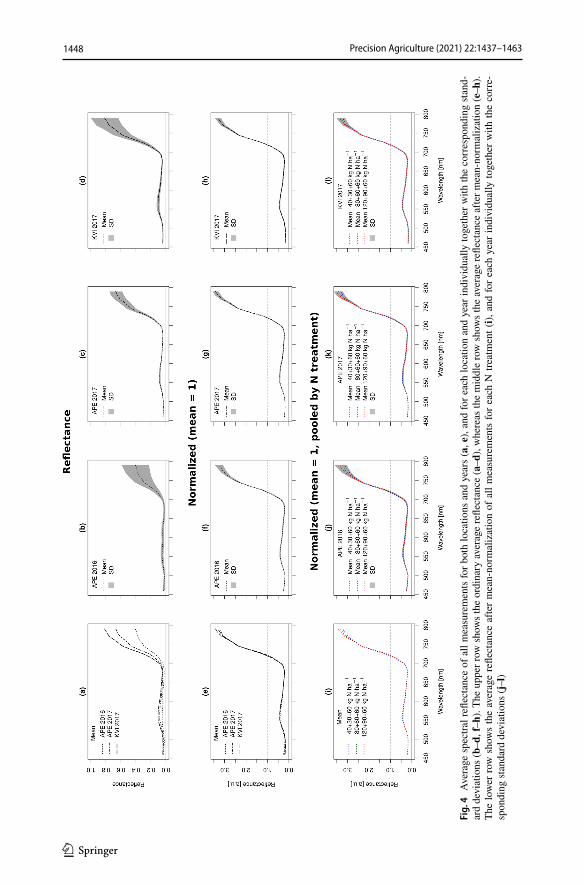
Fig.

4

Ave

rage

spe

ctra

l refl

ecta

nce

of a

ll m

easu

rem

ents

for b

oth

loca

tions

and

yea

rs (a

, e),

and

for e

ach

loca

tion

and

year

indi

vidu

ally

toge

ther

with

the

corr

espo

ndin

g st

and-

ard

devi

atio

ns (b

–d, f

–h).

The

uppe

r row

show

s the

ord

inar

y av

erag

e re

flect

ance

(a–d

), w

here

as th

e m

iddl

e ro

w sh

ows t

he a

vera

ge re

flect

ance

afte

r mea

n-no

rmal

izat

ion

(e–h

). Th

e lo

wer

row

sho

ws

the

aver

age

refle

ctan

ce a

fter m

ean-

norm

aliz

atio

n of

all

mea

sure

men

ts fo

r eac

h N

trea

tmen

t (i),

and

for e

ach

year

indi

vidu

ally

toge

ther

with

the

corr

e-sp

ondi

ng st

anda

rd d

evia

tions

(j–l

)


1 3

Tabl

e 4

Cal

ibra

tion

and

valid

atio

n PP

LSR

mod

el re

sults

for f

resh

(FM

) and

dry

mat

ter y

ield

s (D

M)

a Sele

cted

pow

er o

ptim

izat

ion

para

met

er, γ

[0.5

; 1]

b Num

ber o

f sel

ecte

d co

mpo

nent

s

Cal

ibra

tion

Valid

atio

n

nγa

nCb

R2

RM

SE [k

g ha

−1 ]

RM

SE [%

]n

R2

RM

SE [k

g ha

−1 ]

RM

SE [%

]

FMPo

oled

354

0.99

90.

8325

5015

.135

30.

8423

5814

.2A

PE 2

016

120

0.86

20.

7724

3415

.111

90.

7723

4714

.4A

PE 2

017

900.

925

0.93

1695

12.7

900.

9416

2711

.9K

VI 2

017

144

0.92

50.

8223

7212

.314

40.

7624

9413

.1D

MPo

oled

354

0.96

90.

8154

715

.135

30.

8055

515

.2A

PE 2

016

120

1.00

40.

7757

714

.811

90.

7955

014

.0A

PE 2

017

900.

953

0.92

472

14.2

900.

9147

113

.8K

VI 2

017

144

0.94

40.

8043

812

.514

40.

7745

212

.5


1 3

Tabl

e 5

Cal

ibra

tion

and

valid

atio

n PP

LSR

mod

el re

sults

for c

rude

pro

tein

(CP)

, dry

mat

ter d

iges

tibili

ty (D

MD

), ne

utra

l det

erge

nt fi

bre

(ND

F) a

nd in

dige

stibl

e ne

utra

l det

er-

gent

fibr

e (iN

DF)

a Sele

cted

pow

er o

ptim

izat

ion

para

met

er, γ

[0.5

; 1]

b Num

ber o

f sel

ecte

d co

mpo

nent

sCal

ibra

tion

Valid

atio

n

nγa

nCb

R2

RM

SE [g

10

0 g−

1 DM

]R

MSE

[%]

nR

2R

MSE

[g

100

g−1 D

M]

RM

SE [%

]

CP

Pool

ed18

30.

995

0.69

1.31

11.5

182

0.72

1.32

11.7

APE

201

650

0.99

10.

591.

2512

.750

0.66

1.06

10.9

APE

201

751

1.00

30.

841.

138.

750

0.85

1.25

9.9

KV

I 201

782

0.98

10.

271.

3812

.282

0.27

1.44

12.8

DM

DPo

oled

183

0.63

50.

751.

692.

418

20.

731.

712.

4A

PE 2

016

500.

945

0.50

1.42

2.0

500.

571.

321.

8A

PE 2

017

510.

642

0.84

1.27

1.7

500.

761.

712.

4K

VI 2

017

821.

002

0.88

1.36

1.9

820.

881.

351.

9N

DF

Pool

ed18

30.

916

0.80

2.45

4.4

182

0.77

2.72

4.8

APE

201

650

0.99

30.

931.

572.

750

0.88

2.10

3.6

APE

201

751

0.83

20.

842.

494.

550

0.84

2.56

4.6

KV

I 201

782

0.93

40.

772.

183.

982

0.72

2.48

4.4

iND

FPo

oled

183

0.89

90.

801.

3113

.218

20.

801.

3212

.8A

PE 2

016

500.

784

0.74

1.30

12.3

500.

741.

2811

.9A

PE 2

017

510.

952

0.87

1.22

11.3

500.

791.

5413

.7K

VI 2

017

821.

003

0.84

1.04

11.3

820.

851.

0511

.0


1 3

where n is the number of samples, Pi are the predicted values, Mi are the measured values, and

−

M is the measured values’ arithmetic mean.

Results

Measurements

All hyperspectral measurements were conducted according to schedule. Due to a problem with the Rikola HSI’s memory card, image stacks were not recorded for the first flight mis-sion in APE 2017 (early first cut). As the 60 trial plots were already harvested when the error was noticed, a repetition of the hyperspectral measurements was not possible. Sam-pling of FM and DM yield was successful, except for one erroneous record in APE 2016 that lead to a missing value for one plot (second cut). The measured yields and quality parameters followed an expected distribution and are given in Tables 2 and 3, respectively.

Although fresh matter yields were highest in KVI 2017 (second year of ley), dry matter yields were highest in APE 2016 (first year of ley), indicating a higher plant water con-tent for the KVI 2017 data set. The highest average dry matter yield at a single date was recorded on the normal first cut in APE 2017 (second year of ley). As a result of the vary-ing fertilization treatments, the yields from both locations, APE and KVI, generally exhib-ited a wide range from low yielding to high yielding trial plots. Due to the missing image stacks from the first flight mission in APE 2017, the yields from the early first cut were not included in Table 2.

Quality parameters, especially crude protein content, were also influenced by the differ-ent fertilization treatments and showed a wide variety, following reasonable distributions except for one occasion: The crude protein contents in APE 2017 (second cut) were unusu-ally high, which may be explained by unusually high clover content in the swards of this cut (averaging 23.5 g 100 g−1 DM, data not shown). As for fresh and dry matter yields, the quality parameters from APE 2017 (early first cut) were not included in Table 3 due to the missing image stacks from the flight mission.

(8)RMSE[%] =100

M× RMSE

Fig. 5 Scatter plot of measured vs. predicted validation results for fresh (FM) and dry matter yields (DM), along with the standardized regression coefficients Beta and their standard deviation (SD) for the general PPLSR models


1 3

Pre‑processed data

The processed ortho-image hypercubes and the DSMs showed an average ground sam-ple distance (GSD) of 37 mm. The average residual RMSE of the GCP 3D locations was 47 mm. The plot-wise extracted and resampled reflectance spectra exhibited a general trend of differences in magnitude between the locations and years. Mean-normalization removed this trend and is displayed as examples for the average spectral reflectance of the measure-ments aggregated by location and year Fig. 4.

Fig. 6 Scatter plot of measured vs. predicted validation results for crude protein (CP), dry matter digest-ibility (DMD), neutral detergent fibre (NDF) and indigestible neutral detergent fibre (iNDF), along with the standardized regression coefficients Beta and their standard deviation (SD) for the general PPLSR models

Fig. 7 Dominant wavebands of the general PPLSR models for fresh (FM) and dry matter yields (DM), crude protein (CP), dry matter digestibility (DMD), neutral detergent fibre (NDF) and indigestible neutral detergent fibre (iNDF)


1 3

Tabl

e 6

Val

idat

ion

of S

LR m

odel

resu

lts w

ith N

DV

I, R

EIP,

and

PH

as p

redi

ctor

s for

fres

h (F

M) a

nd d

ry m

atte

r yie

lds (

DM

)

a Not

sign

ifica

nt (p

> 0.

05)

Valid

atio

nN

DV

IR

EIP

PH

nR

2R

MSE

[kg

ha−

1 ]R

MSE

[%]

R2

RM

SE [k

g ha

−1 ]

RM

SE [%

]R

2R

MSE

[kg

ha−

1 ]R

MSE

[%

]

FMPo

oled

353

0.05

5692

34.3

n.s.a

n.s.a

n.s.a

0.21

5203

31.3

APE

201

611

9n.

s.an.

s.an.

s.a0.

0847

1928

.90.

3739

7224

.3A

PE 2

017

900.

2855

4840

.7n.

s.an.

s.an.

s.a0.

6943

8232

.2K

VI 2

017

144

0.08

4940

25.9

0.16

4720

24.8

n.s.a

n.s.a

n.s.a

DM

Pool

ed35

30.

1011

8132

.30.

0112

4133

.90.

2311

0030

.1A

PE 2

016

119

0.09

1156

29.4

0.06

1171

29.8

0.25

1052

26.7

APE

201

790

0.27

1392

40.7

n.s.a

n.s.a

n.s.a

0.67

1072

31.4

KV

I 201

714

40.

0990

224

.90.

1487

524

.2n.

s.an.

s.an.

s.a


1 3

Tabl

e 7

Val

idat

ion

of S

LR m

odel

resu

lts w

ith N

DV

I, R

EIP,

and

PH

as

pred

icto

rs fo

r cru

de p

rote

in (C

P), d

ry m

atte

r dig

estib

ility

(DM

D),

neut

ral d

eter

gent

fibr

e (N

DF)

and

in

dige

stibl

e ne

utra

l det

erge

nt fi

bre

(iND

F)

a Not

sign

ifica

nt (p

> 0.

05)

Valid

atio

nn

ND

VI

REI

PPH

R2

RM

SE [g

10

0 g−

1 DM

]R

MSE

[%]

R2

RM

SE [g

10

0 g−

1 DM

]R

MSE

[%]

R2

RM

SE [g

10

0 g−

1 DM

]R

MSE

[%]

CP

Pool

ed18

20.

092.

4021

.40.

202.

2620

.10.

262.

2019

.6A

PE 2

016

500.

581.

2112

.40.

151.

7417

.9n.

s.an.

s.an.

s.a

APE

201

750

0.48

2.52

19.9

0.13

3.06

24.2

n.s.a

n.s.a

n.s.a

KV

I 201

782

n.s.a

n.s.a

n.s.a

0.04

1.69

15.0

0.09

1.64

14.5

DM

DPo

oled

182

0.11

3.14

4.4

n.s.a

n.s.a

n.s.a

0.08

3.18

4.4

APE

201

650

n.s.a

n.s.a

n.s.a

0.23

1.81

2.5

n.s.a

n.s.a

n.s.a

APE

201

750

0.33

3.01

4.2

n.s.a

n.s.a

n.s.a

0.47

2.82

3.9

KV

I 201

782

0.12

3.65

5.1

0.03

3.87

5.4

n.s.a

n.s.a

n.s.a

ND

FPo

oled

182

0.07

5.48

9.7

0.01

5.67

10.0

0.29

4.81

8.5

APE

201

650

n.s.a

n.s.a

n.s.a

n.s.a

n.s.a

n.s.a

0.60

3.94

6.8

APE

201

750

0.35

5.49

9.9

0.02

6.48

11.7

0.45

5.58

10.1

KV

I 201

782

0.05

4.65

8.2

0.18

4.33

7.7

n.s.a

n.s.a

n.s.a

iND

FPo

oled

182

0.19

2.72

26.3

n.s.a

n.s.a

n.s.a

0.15

2.81

27.2

APE

201

650

0.30

2.17

20.2

n.s.a

n.s.a

n.s.a

0.25

2.26

21.0

APE

201

750

0.37

2.84

25.2

n.s.a

n.s.a

n.s.a

0.49

2.75

24.4

KV

I 201

782

0.12

2.62

27.6

n.s.a

n.s.a

n.s.a

n.s.a

n.s.a

n.s.a


1 3

Model outcomes

The PPLSR model results for forage yield and quality are given in Tables 4 and 5, respec-tively. Both tables show the calibration and validation results for one generalized (i.e. using pooled datasets) and three individual models for each combination of location and year. Although the validation results are most important in terms of model generalization, the calibration results are shown for completeness. It should be emphasized that outliers were not removed from any of the models.

All PPLSR models for the prediction of fresh and dry matter yields showed relatively low RMSEs of validation, with models that were based on data subsets achieving slightly higher prediction accuracies than the general models for fresh matter (RMSE of 14.2%, 2358 kg FM ha−1) and dry matter prediction (RMSE of 15.2%, 555 kg DM ha−1). All mod-els followed a similar trend, exhibiting γ values in the upper range (0.86–1.00), empha-sizing the importance of correlation between predictors and dependent variables. With 9 components, both general models were more complex than the models that were based on data subsets (2–5 selected components).

Wavebands in the RE and NIR region contributed more to the prediction of fresh and dry matter yields than those in the VIS region Fig. 5.

The prediction of quality parameters with PPLSR models followed a similar trend to the prediction of fresh and dry matter. General models achieved slightly lower predictive performances than prediction models built on data subsets (Table 5). Again, general mod-els were more complex and featured a higher number of selected components (5–9) and the models for the prediction of crude protein concentration, neutral detergent fibre and indigestible neutral detergent fibre showed γ values close to 1 (γ = 0.89–0.99). In contrast, the general model for the prediction of dry matter digestibility had a much lower γ value (0.63), indicating that larger weight was given to predictors with high variance. It is note-worthy, that the model for the prediction of crude protein content that was solely built on the KVI 2017 data set, explained less than 30% of the variation in measured crude protein (R2 = 0.27).

Wavebands in the RE and NIR region contributed mainly to the prediction of crude protein content, wavebands in the NIR region to the prediction of dry matter digestibility, wavebands in the RE region to the prediction of neutral detergent fibre, and wavebands in the green, RE and NIR region to the prediction of indigestible neutral detergent fibre Fig. 6. The scatter plot for crude protein content estimation shows a tendency towards over-estimation of lower and underestimation of higher crude protein contents, which might result from the unusually high clover contents in the second cut of the APE 2017 data set and the unexplained variation within the KVI 2017 data set.

Figure 7 summarizes the centre wavelengths λ of those wavebands that were found to be dominant contributors to the general prediction models. Only four of the dominant wavebands were in the VIS part of the electromagnetic spectrum, and they were either used in the prediction of dry matter yields (λ = 520 nm), neutral detergent fibre content (λ = 695 nm), or indigestible neutral detergent fibre content (λ = 520 nm and 530 nm). All other dominating wavebands were in the RE and NIR region.

The SLR model results for forage yield and quality are given in Tables 6 and 7, respectively. The prediction performance of these models, based on the vegetation indi-ces and the plant height, was generally poor.

Although model predictions of fresh and dry matter yields based on the APE 2017 data set with PH as predictor variable achieved coefficients of determination of almost


1 3

0.7, the RMSEs of validation were low compared with the performances of the corre-sponding PPLSR models. None of the SLR models predicted fresh matter yields with an RMSE lower than 24.3% (3972 kg FM ha−1) and dry matter yields with an RMSE lower than 24.1% (875 kg DM ha−1).

The prediction of quality parameters with the SLR models followed a very similar pat-tern to the prediction of fresh and dry matter yields. Only one SLR model obtained results being reasonably close to the corresponding PPLSR model in terms of predictive power; the model predicting crude protein content based on the APE 2016 data using NDVI as predictor. This NDVI model achieved an RMSE of 12.4% (1.21 g 100 g−1 DM), whereas the PPLSR model achieved an RMSE of 10.9% (1.06 g 100 g−1 DM).

Discussion

The PPLSR modelling approach returned models that achieved high prediction accuracies for both forage yield and quality estimates. In contrast, SLR models based on the indices NDVI, REIP and PH as predictor variables did not achieve satisfactory prediction accura-cies, except for some models that were based on subsets of the data. Both the multivariate and the simple linear regressions revealed that subset models, calibrated on data from one location and year, performed better than models based on pooled data. It should, however, be emphasized that the subset models were validated on subsets of the data (i.e. data from the same field and year, but not used in the calibration). When the subset models were tested on pooled data, their prediction accuracies were poor (not shown). In other words, the subset models were less generalizable than the models based on the pooled data.

Generalizability may be expressed as a model’s ability to perform well when applied to new conditions, while maintaining the same set of explanatory variables and parameters (Patton et al. 2015). The generalizability of a model depends on many factors, such as type of data, the degree of variation between the environment in which the calibrations were performed and the new conditions, and the size and quality of the calibration data. When predicting yields and yield quality in spring wheat utilizing hyperspectral data, Øvergaard et al. (2013) showed that the generalizability of their models (expressed as the normalized RMSE of validation for an independent dataset with n = 144) increased with increasing size of the calibration dataset from n = 160 to n = 832. The authors attributed this effect largely to the increasing variation in the calibration data, when more years and sites were included.

As prediction models based on large datasets are more favourable in terms of generaliz-ability than models calibrated on smaller data sets, the discussion focus on the PPLSR pre-diction models that were based on the pooled data sets. Nevertheless, the data sets contain measurements on only one of many common grassland species compositions. Hence, apart from other aforementioned reasons, the resulting PPLSR prediction models may be limited in terms of generalizability when used in other grassland types.

Within grassland research, studies that have utilized airborne hyperspectral imaging with data sets at sample sizes that allow statements on the generalizability of the calibrated models are scarce. Model performance in the current study, here defined as the relative error of prediction (i.e. normalized RMSE of validation), has therefore been compared to some studies that have presented models with a limited generalizability, i.e. with smaller number of calibration and validation samples, sample locations and years included. There exist, however, more comprehensive studies that have utilized handheld hyperspectral sens-ing technologies, and these were used as additional benchmarks. It is noteworthy that these


1 3

handheld instruments commonly enable a much higher spectral and radiometric resolu-tion at a wider spectral range, from VIS to shortwave infrared (SWIR), than hyperspectral equipment suitable for mounting on UAVs (such as the Rikola HSI used in this study). Measurements in the shortwave infrared range are beneficial in terms of multivariate model calibration for quality parameters, such as proteins, cellulose, and lignin, since these prop-erties show absorption of radiation in the SWIR part of the electromagnetic spectrum (Cur-ran 1989).

Forage yield prediction

The PPLSR model presented was able to predict fresh matter yields at a high accuracy. With a prediction error of 14.2%, it performed better than the model of Capolupo et al. (2015; 17.6%, n = 120), who used PLSR and leave-one-out cross validation (LOO-CV) on data from experimental grassland swards, fertilized with N levels ranging from 0 kg to 340 kg annual N ha−1. The difference between PPLSR and PLSR is that the former includes a power optimization parameter γ, which has the ability to focus the algorithm. Using a γ-value of 0.5, the PPLSR degenerates to the PLSR-solution, which focus on the covariance of the data (i.e. by finding the multidimensional direction in the predic-tor space that explains the maximum multidimensional variance direction in the space of the dependent variables). When increasing the γ-value above 0.5, the correlation between predictors and dependent variables is given gradually more weight in the algorithm. In all PPLSR-models presented, the automatically fitted γ values were larger than 0.5, and thereby obtaining higher prediction accuracies than what had been the case when using a PLS approach. The finding that a modelling approach based on PPLSR was superior to a PLSR-approach, was also reported by Øvergaard et al. (2013, 2010), when analysing yields and quality in spring wheat.

Whereas Capolupo et al. (2015) used hyperspectral data acquired by a UAV, a method comparable to the current study, Schut et al. (2006) utilized a sensor system consisting of three active hyperspectral sensors mounted on a mobile ground platform. With a spa-tial resolution of measured reflectance on the soil surface of up to 1.39 by 152 mm, they reported prediction errors of fresh matter herbage yield of 7–18%, when using PLSR and leave-k-out cross validation (LKO-CV, n = 76–413) on pure and mixed perennial ryegrass (Lolium perenne L.) and white clover (Trifolium repens L.) swards with N applications of 0–450 kg annual N ha−1. In spite of the large differences between the current study and that of Schut et al. (2006) in terms of spatial resolution and type of sensors, the results were within the same range. Considering that the use of UAV represents a very efficient method for data acquisition compared to most ground-based approaches, the results appear promising.

Dry matter yields were also predicted at a high accuracy, with an error of 15.2%. This is comparable to that reported by Capolupo et al. (2015; 15.9%), who appeared to improve their accuracy noticeably when predicting DM yields compared with FM yields. In con-trast, the model performance in this study became slightly poorer when predicting DM yields. In the ground based approach of Schut et al. (2006), the authors reported the same phenomenon, as their relative error increased from 7–18% to 8–22%, when moving from FM to DM yield predictions. Presumably, FM yield predictions may obtain higher accura-cies when compared to DM yield predictions since spectral signals observed from the sen-sor may be a more direct measure of the plants’ FM than DM. This assumption is supported


1 3

by Wang et al. (2011). They studied spectral reflectance from green leaves combining field data and simulations with the PROSPECT-model and reported that leaf internal structure is a confounding factor for dry matter estimation over the entire NIR-spectrum. The findings of this study could also be indirectly related to water content. Carter (1991) found second-ary effects of water (i.e. effects not resulting solely from the radiative properties of water) in leaves throughout the 400–2500 nm wavelength range.

Zhou et al. (2019) utilized a hand-held spectrometer in combination with support vec-tor machine (SVM) regressions to estimate selected forage crop properties. Splitting their data of mixtures of different grass and legume species (n = 377) in two, corresponding to a 2:1 ratio for the size of the calibration and the validation data set (C:V-ratio), they obtained an accuracy of their DM forage biomass estimates of 14.1%. Other studies have indicated that there may be a potential to achieve even higher accuracies by inclusion of additional predictor variables. Näsi et al. (2018) and Oliveira et al. (2019) reported prediction errors in the range from 6% to 12.5%, when using random forest (RF) regression models and LOO-CV based on the full spectrum (up to 36 wavebands) and adding 3D features and vegetation indices as predictors. Viljanen et al. (2018) found an error of 12.7% with a mul-tiple linear regression (MLR) model and LOO-CV, using plant height, vegetation indices and RGB information as predictors. These three studies, however, used data from the same field trial, and the models were run on very small data sets (n = 24) of timothy dominated swards, mixed with meadow fescue. Fertilizer was applied with six N levels from 0 kg N ha−1 to 150 kg N ha−1 and the growth was monitored over a short period of 23 days, only. In order to conclude on any possible benefits of using additional predictor variables to those obtained by spectral reflection, such studies need to be validated with far more com-prehensive datasets.

In this study, the most dominant wavebands were observed within the spectral regions of the red-edge inflection point and the NIR, for both models predicting FM and DM yields. The RE region (i.e. the region around the point of maximum slope in the reflectance spec-tra of green leaves, which normally occurs between 680 nm and 750 nm; Gitelson et al. 1996) is long known to be strongly correlated with the chlorophyll concentration of green biomass (e.g. Pinar and Curran 1996). In contrast, the NIR reflection depends on structural components like the amount and thickness of cell walls and inter-cellular spaces (Gausman 1977; Knipling 1970), and increases normally with increasing biomass density. Wavebands in the chlorophyll absorption areas of VIS (i.e. with peaks at 430 nm, 460 nm, 640 nm and 660 nm; Curran 1989) did not appear to affect the models much, even though VIS radiation is mainly influenced by leaf pigments (Gates et al. 1965; Guyot et al. 1992).

Forage quality prediction

The selected PPLSR-model, estimating crude protein (CP) content, achieved a high accu-racy with an error of 11.7%. This is comparable with the results reported by Wijesingha et al. (2020), who obtained an accuracy of 10.6% when gathering data from eight grass-land sites with different management practices and species compositions, using a UAV-borne hyperspectral camera in combination with SVM regressions with a C:V-ratio of 4:1 (n = 194). The authors were surprised to find that the reflectance at wavelength 718 nm was most fundamental for their best CP-model, since this band is not related to any foliar chem-ical absorption feature, such as protein. The findings of this study support, however, that reported by Wijesingha et al. (2020), as the most dominating bands in the CP-model had centre wavelengths at 720 nm and 725 nm. All these wavelengths are located within the


1 3

region of the red-edge inflection point, which is known for its strong correlation with leaf chlorophyll and nitrogen content (Fava et al. 2009; Gitelson et al. 2003). Although the RE region does not contain typical protein absorption bands, the findings may be explained by a more indirect effect: almost 80 years ago it was established that the chlorophyll-protein compound in green leaves contains a significant proportion (around 16%) of the total leaf protein content (Smith 1941).

Capolupo et al. (2015) reported an even smaller prediction error when estimating CP (9.7%), using PLSR and LOO-CV. They found correlations above 0.5 (i.e. Pearson’s r) between spectral bands of the hyperspectral dataset and crude protein for the entire range from 450 nm to 720 nm, with peaks around 460 nm and 680 nm. Pullanagari et al. (2018), using a pushbroom hyperspectral imaging system mounted on a manned aircraft, reported an absolute prediction error of 2.2 g CP 100 g−1 DM (corresponding to a relative error of 13.5%), when using RF regressions and a C:V-ratio of 3:2 (n = 150). The underlying data was sampled from 150 sites with perennial ryegrass and white clover as the dominant spe-cies. They identified distinct spectral features in the SWIR region as main contributors. These features lie outside the measurement range of the sensor used in the current study, but the findings show that it is possible to achieve a comparably high accuracy of CP-pre-dictions using the RE-NIR region only. Using ground based field spectroscopy, Pullanagari et al. (2012; PLSR with 1:1 C:V-ratio, n = 214, mainly perennial ryegrass and white clover grassland), Schut et al. (2006, n = 76–413) and Zhou et al. (2019, n = 377) reported predic-tion errors of 11.3%, 7–11%, and 15.6%, respectively. These findings illustrate that with the authors’ current knowledge, there appears to be no distinct difference in terms of modelling accuracy of crude protein predictions in forage biomass, whether the reflectance data is acquired from airborne or from ground-based sensors.

In this study, dry matter digestibility (DMD) content was predicted at a very high accu-racy, with an error of only 2.4%. The wavebands which dominated the prediction model, were exclusively within the NIR range (770–790 nm), a region known for its high cor-relation with plant structural components. The authors were not able to find any directly comparable reference studies. However, Pullanagari et al. (2012) predicted the content of organic matter digestibility (OMD) in mixed pastures (i.e. commercial New Zealand pas-tures), using a hand-held spectrometer and a probe (containing an active light source). They reported a prediction error of 5.1% but did not present any dominant wavebands for OMD.

As for DMD, the prediction of neutral detergent fibre (NDF) content resulted in very accurate estimates, with an error of only 4.8%. In comparison, Schut et al. (2006) achieved an even smaller error (3%), whereas Pullanagari et al. (2012) reported a somewhat larger error (10.6%). In both these studies, the prediction models were based on data from ground-based field spectroscopy and PLSR. In the current study, there was a strong relationship between reflectance in the RE-NIR region and NDF, which is in line with Pullanagari et al. (2012), who found that wavelengths around 805 nm (i.e. NIR-region) were important when predicting the same forage quality parameter.

Indigestible neutral detergent fibre (iNDF) was estimated with a prediction error of 12.8%, thus significantly larger than that of NDF. The authors cannot explain the reason for this reduction in accuracy. In contrast to the prediction model for NDF, the iNDF predic-tion model is based on dominant wavebands in the VIS (520–530 nm) and in the RE-NIR range (735 nm and 770 nm). To the authors’ knowledge, there exists no reference studies for comparison using wavebands in similar spectral regions.


1 3

Data preparation

In the current study, all images and extracted features underwent thorough pre-pro-cessing routines in order to secure high geometric, spectral and radiometric quality of the modelling data. Data preparation is essential in terms of generating sound model input data (Aasen and Bolten 2018; Aasen et al. 2018), and the need for such routines increases as the measurement methods get more advanced. Even though the pre-pro-cessing in this study was relatively comprehensive, it was still necessary to perform a z-transformation of the extracted and resampled reflectance spectra to remove a general trend of differences in magnitude that was apparent between spectra originating from different locations and years.

The Euclidean distance of the spectra matrices was used as selection criterion for splitting the data into equally sized calibration and validation data sets for modelling. This maximized the variation within the data sets, and thereby enhanced the potential of model generalizability. The size of both calibration and validation data sets were unusu-ally large, and outliers were not removed from them. The overall high accuracy of the prediction models thus highlights the strong potential of the PPLSR method. It should be emphasized, that the model selection approach in this study was based on a combina-tion of the selection strategies of Indahl (2005) and Mevik and Wehrens (2007), which should be regarded as a rather conservative approach.

Conclusions

Combining UAV-borne hyperspectral imaging spectroscopy with multivariate statistics is a promising approach for rapid and non-destructive in-season forage yield and qual-ity estimation. The use of models that utilize the full spectrum/many bands as potential predictors appear to be superior to model-approaches based on a few bands, though this was shown for SLR models with NDVI and REIP as predictor variables, only. High accuracies in terms of yield and quality predictions do not, however, require a spec-trum reaching beyond the VIS–NIR-region. The hyperspectral imager used in this study, which measured 29 wavebands in the range from 450 nm to 800 nm, obtained prediction results comparable or even better than those reported by authors that used field spec-troscopy with hundreds of wavebands in the range from 350 nm to 2500 nm. A model’s ability to perform well when applied to new conditions generally increases with increas-ing size and variation in the calibration data set, and many studies suffer from too lim-ited data sets to provide generalizable models. Regardless of the size of the calibration data, however, thorough pre-processing of hyperspectral imagery is a prerequisite in order to secure high data integrity and model accuracy.

Acknowledgements This study has been conducted as part of the project Use of remote sensing for increased precision in forage production (Research Council of Norway, Project Number 244251), funded by Forskningsmidlene for jordbruk og matindustri. We profoundly thank our NIBIO colleagues Anne Langerud, Håvard Lindgaard and Jan Thomsen for carrying out the field experiments, Bea Blomlie and Tor Lunnan for performing the laboratory NIRS analyses, and Maximilian Pircher for executing the UAV missions.

Funding Open Access funding provided by Norwegian Institute of Bioeconomy Research. This study has been conducted as part of the project Use of remote sensing for increased precision in forage production


1 3

(Research Council of Norway, Project Number 244251), funded by Forskningsmidlene for jordbruk og matindustri.

Data availability Not applicable.

Code availability Not applicable.

Compliance with ethical standards

Conflict of interest Not applicable.

Ethical approval The work with ethics at Norwegian Institute of Bioeconomy Research (NIBIO) is guided by the Research Ethics Act. The research and activities in this study do not conflict with NIBIO’s ethical guidelines, which comprise personal and business conduct, research ethics, and good scientific and publica-tion practice.

Consent to participate Not applicable.

Consent for publication Not applicable.

Open Access This article is licensed under a Creative Commons Attribution 4.0 International License, which permits use, sharing, adaptation, distribution and reproduction in any medium or format, as long as you give appropriate credit to the original author(s) and the source, provide a link to the Creative Com-mons licence, and indicate if changes were made. The images or other third party material in this article are included in the article’s Creative Commons licence, unless indicated otherwise in a credit line to the material. If material is not included in the article’s Creative Commons licence and your intended use is not permitted by statutory regulation or exceeds the permitted use, you will need to obtain permission directly from the copyright holder. To view a copy of this licence, visit http:// creat iveco mmons. org/ licen ses/ by/4. 0/.

References

Aasen, H., & Bolten, A. (2018). Multi-temporal high-resolution imaging spectroscopy with hypespectral 2D imagers – From theory to application. Remote Sensing of Environment, 205, 374–389.

Aasen, H., Honkavaara, E., Lucieer, A., & Zarco-Tejada, P. (2018). Quantitative remote sensing at ultra-high resolution with UAV spectroscopy: A review of sensor technology, measurement procedures, and data correction workflows. Remote Sensing, 10(7), 1091.

Capolupo, A., Kooistra, L., Berendonk, C., Boccia, L., & Suomalainen, J. (2015). Estimating plant traits of Grasslands from UAV-acquired hyperspectral images: A comparison of statistical approaches. ISPRS International Journal of Geo-Information, 4(4), 2792–2820.

Carter, G. A. (1991). Primary and secondary effects of water content on the spectral reflectance of leaves. American Journal of Botany, 78(7), 916–924.

Cho, M. A., Skidmore, A., Corsi, F., van Wieren, S. E., & Sobhan, I. (2007). Estimation of green grass/herb biomass from airborne hyperspectral imagery using spectral indices and partial least squares regres-sion. International Journal of Applied Earth Observation and Geoinformation, 9(4), 414–424.

Curran, P. J. (1989). Remote sensing of foliar chemistry. Remote Sensing of Environment, 30(3), 271–278.Fava, F., Colombo, R., Bocchi, S., Meroni, M., Sitzia, M., Fois, N., et al. (2009). Identification of hyperspec-

tral vegetation indices for Mediterranean pasture characterization. International Journal of Applied Earth Observation and Geoinformation, 11(4), 233–243.

Fu, Y., Yang, G., Wang, J., Song, X., & Feng, H. (2014). Winter wheat biomass estimation based on spectral indices, band depth analysis and partial least squares regression using hyperspectral measurements. Computers and Electronics in Agriculture, 100, 51–59.

Fystro, G., & Lunnan, T. (2006). Analysar av grovfôrkvalitet på NIRS (Analyses of forage quality by NIRS). In A. Ø. Kristoffersen (Ed.), Proceedings of the Plantemøtet Østlandet 2006. Bioforsk FOKUS 1(3), 180–182.

Gates, D. M., Keegan, H. J., Schleter, J. C., & Weidner, V. R. (1965). Spectral properties of plants. Applied Optics, 4(1), 11–20.

http://creativecommons.org/licenses/by/4.0/


1 3

Gausman, H. (1977). Reflectance of leaf components. Remote Sensing of Environment, 6(1), 1–9.Geipel, J., & Korsaeth, A. (2017). Hyperspectral aerial imaging for grassland yield estimation. In J. A. Tay-

lor, D. Cammarano, A. Prashar, A. Hamilton (Eds.), Proceedings of the 11th European Conference on Precision Agriculture. Advances in Animal Biosciences, 8(2), 770–775.

Gitelson, A. A., Gritz, Y., & Merzlyak, M. N. (2003). Relationships between leaf chlorophyll content and spectral reflectance and algorithms for non-destructive chlorophyll assessment in higher plant leaves. Journal of Plant Physiology, 160(3), 271–282.

Gitelson, A. A., Merzlyak, M. N., & Lichtenthaler, H. K. (1996). Detection of red edge position and chlo-rophyll content by reflectance measurements near 700 nm. Journal of Plant Physiology, 148(3–4), 501–508.

Guyot, G., Baret, F., & Jacquemoud, S. (1992). Imaging spectroscopy for vegetation studies. In F. Toselli & J. Bodechtel (Eds.), Imaging spectroscopy: Fundamentals and prospective applications (pp. 145–165). Dordrecht, The Netherlands: Kluwer Academic Publishers.

Indahl, U. (2005). A twist to partial least squares regression. Journal of Chemometrics, 19(1), 32–44.Jakob, S., Zimmermann, R., & Gloaguen, R. (2017). The Need for accurate geometric and radiometric cor-

rections of drone-borne hyperspectral data for mineral exploration: MEPHySTo – A toolbox for pre-processing drone-borne hyperspectral data. Remote Sensing, 9(1), 88.

Knipling, E. B. (1970). Physical and physiological basis for the reflectance of visible and near-infrared radiation from vegetation. Remote Sensing of Environment, 1(3), 155–159.

Kusnierek, K., & Korsaeth, A. (2015). Simultaneous identification of spring wheat nitrogen and water status using visible and near infrared spectra and Powered Partial Least Squares Regression. Com-puters and Electronics in Agriculture, 117, 200–213.

Mevik, B.-H., & Wehrens, R. (2007). The pls package: principal component and partial least squares regression in R. Journal of Statistical Software, 18(1), 1–23.

Nordskog, B., Bakken, A. K., & Hole, H. (2018). Jordtemperatur og spredning av husdyrgjødsel - Utred-ning av om jordtemperatur kan brukes som skranke for spredning av husdyrgjødsel på eng i Far-sund kommune (Soil temperature and spreading of liquid manure – Investigation of whether soil temperature can be used as threshold for spreading liquid manure in grasslands in Farsund munici-pality). NIBIO rapport, 4(72), 1–18.

Näsi, R., Viljanen, N., Oliveira, R., Kaivosoja, J., Niemeläinen, O., Hakala, T., et al. (2018). Optimizing radiometric processing and feature extraction of drone based hyperspectral frame format imagery for estimation of yield quantity and quality of a Grass Sward. ISPRS – International Archives of the Photogrammetry, Remote Sensing and Spatial Information Sciences, XLII–3, 1305–1310.

Oliveira, R. A., Näsi, R., Niemeläinen, O., Nyholm, L., Alhonoja, K., Kaivosoja, J., et al. (2019). Assessment of RGB and hyperspectral UAV remote sensing for grass quantity and quality estima-tion. ISPRS – International Archives of the Photogrammetry, Remote Sensing and Spatial Informa-tion Sciences, XLII-2/W13, 489–494.

Øvergaard, S. I., Isaksson, T., Kvaal, K., & Korsaeth, A. (2010). Comparisons of two hand-held, multi-spectral field radiometers and a hyperspectral airborne imager in terms of predicting spring wheat grain yield and quality by means of powered partial least squares regression. Journal of Near Infra-red Spectroscopy, 18(4), 247–261.

Øvergaard, S. I., Isaksson, T., & Korsaeth, A. (2013). Prediction of wheat yield and protein using remote sensors on plots – Part I: Assessing near infrared model robustness for year and site variations. Journal of Near Infrared Spectroscopy, 21(2), 117–131.

Patton, A. P., Zamore, W., Naumova, E. N., Levy, J. I., Brugge, D., & Durant, J. L. (2015). Transfer-ability and generalizability of regression models of ultrafine particles in urban neighborhoods in the Boston area. Environmental Science and Technology, 49(10), 6051–6060.

Pinar, A., & Curran, P. J. (1996). Technical note grass chlorophyll and the reflectance red edge. Interna-tional Journal of Remote Sensing, 17(2), 351–357.

Pullanagari, R. R., Kereszturi, G., & Yule, I. (2018). Integrating airborne hyperspectral, topographic, and soil data for estimating pasture quality using recursive feature elimination with random forest regression. Remote Sensing, 10(7), 1117.

Pullanagari, R. R., Kereszturi, G., & Yule, I. (2016). Mapping of macro and micro nutrients of mixed pastures using airborne AisaFENIX hyperspectral imagery. ISPRS Journal of Photogrammetry and Remote Sensing, 117, 1–10.

Pullanagari, R. R., Yule, I. J., Tuohy, M. P., Hedley, M. J., Dynes, R. A., & King, W. M. (2012). In-field hyperspectral proximal sensing for estimating quality parameters of mixed pasture. Precision Agri-culture, 13(3), 351–369.

Python Software Foundation. (2021). Python Language Reference, version 2.7. Available at https:// www. python. org.

https://www.python.org

https://www.python.org


1 3

QGIS Development Team. (2021). QGIS geographic information system, version 2.18.5. Available at https:// www. qgis. org.

R Core Team. (2021). R: A language and environment for statistical computing, version 3.2.3. Available at https:// www.r- proje ct. org.

Rouse, J. W., Jr., Haas, R. H., Schell, J. A., & Deering, D. W. (1974). Monitoring vegetation systems in the great plains with ERTS. In S. C. Freden, E. P. Mercanti, & M. A. Becker (Eds.), Third earth resources technology satellite-1 symposium volume I: Technical presentations (pp. 309–317). Washington, DC: NASA.

Safari, H., Fricke, T., & Wachendorf, M. (2016). Determination of fibre and protein content in heteroge-neous pastures using field spectroscopy and ultrasonic sward height measurements. Computers and Electronics in Agriculture, 123, 256–263.

Schellberg, J., & Verbruggen, E. (2014). Frontiers and perspectives on research strategies in grassland technology. Crop and Pasture Science, 65(6), 508–523.

Schellberg, J., Hill, M. J., Gerhards, R., Rothmund, M., & Braun, M. (2008). Precision agriculture on grassland: Applications, perspectives and constraints. European Journal of Agronomy, 29(2–3), 59–71.

Schut, A. G. T., van der Heijden, G. W. A. M., Hoving, I., Stienezen, M. W. J., van Evert, F. K., & Meule-man, J. (2006). Imaging spectroscopy for on-farm measurement of grassland yield and quality. Agron-omy Journal, 98(5), 1318–1325.

Smith, E. L. (1941). The chlorophyll-protein compound of the green leaf. Journal of General Physiology, 24(5), 565–582.

Viljanen, N., Honkavaara, E., Näsi, R., Hakala, T., Niemeläinen, O., & Kaivosoja, J. (2018). A novel machine learning method for estimating biomass of grass swards using a photogrammetric canopy height model, images and vegetation indices captured by a drone. Agriculture, 8(5), 70.

Wachendorf, M., Fricke, T., & Möckel, T. (2018). Remote sensing as a tool to assess botanical composition, structure, quantity and quality of temperate grasslands. Grass and Forage Science, 73(1), 1–14.

Wang, L., Qu, J. J., Hao, X., & Hunt, E. R. H. Jr. (2011). Estimating dry matter content from spectral reflectance for green leaves of different species. International Journal of Remote Sensing, 32(22), 7097–7109.

Weiss, M., Jacob, F., & Duveiller, G. (2020). Remote sensing for agricultural applications: A meta-review. Remote Sensing of Environment, 236, 111402.

Wijesingha, J., Astor, T., Schulze-Brüninghoff, D., Wengert, M., & Wachendorf, M. (2020). Predicting for-age quality of Grasslands using UAV-borne imaging spectroscopy. Remote Sensing, 12(1), 126.

Zhou, Z., Morel, J., Parsons, D., Kucheryavskiy, S. V., & Gustavsson, A.-M. (2019). Estimation of yield and quality of legume and grass mixtures using partial least squares and support vector machine analysis of spectral data. Computers and Electronics in Agriculture, 162, 246–253.

Publisher’s Note Springer Nature remains neutral with regard to jurisdictional claims in published maps and institutional affiliations.

https://www.qgis.org

https://www.r-project.org

forage yield and quality estimation by means of uav and

Documents