For Wednesday

• Read Chapter 11, sections 1-2

• Program 2 due

Program 2

• Any questions?

Probability Review

Problems with Probabilistic Reasoning

• If no assumptions of independence are made, then an exponential number of parameters is needed for sound probabilistic reasoning.

• There is almost never enough data or patience to reliably estimate so many very specific parameters.

• If a blanket assumption of conditional independence is made, efficient probabilistic reasoning is possible, but such a strong assumption is rarely warranted.

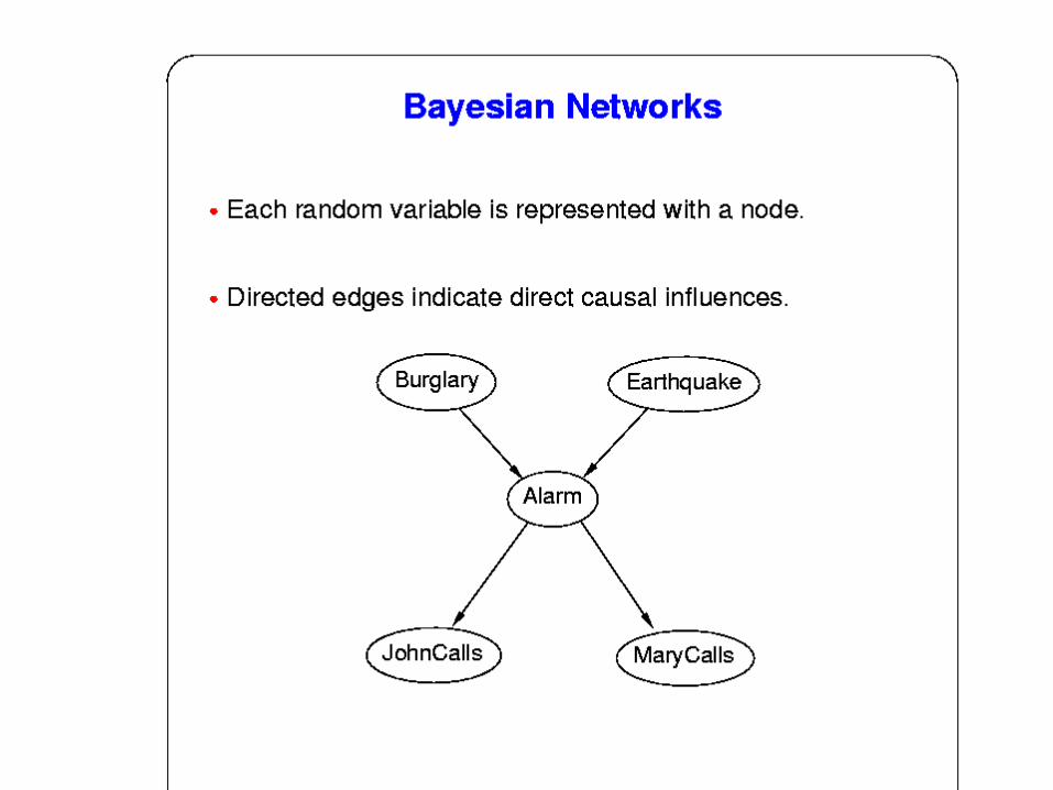
Bayesian Networks

• Bayesian networks (belief network, probabilistic network, causal network) use a directed acyclic graph (DAG) to specify the direct (causal) dependencies between variables and thereby allow for limited assumptions of independence.

• The number of parameters need for a Bayesian network are generally much less compared to making no independence assumptions.

More on CPTs

• Probability of false is not given since rows must sum to 1.

• Requires 10 parameters rather than 25 =32 (actually only 31 since all 32 values must sum to 1)

• Therefore, the number of probabilities needed for a node is exponential in the number of parents (the fan in).

Noisy-Or Nodes• To avoid specifying the complete CPT, special nodes that make

assumptions about the style of interaction can be used. • A noisy or node assumes that the parents are independent causes that are

noisy, i.e. there is some probability that they will not cause the effect. • The noise parameter for each cause indicates the probability it will not

cause the effect. • Probability that the effect is not present is the product of the noise

parameters of all the parent nodes that are true (since independence is assumed). P(Fever|Cold) =0.4,P(Fever|Flu) =0.8,P(Fever| Malaria)=0.9

P(Fever | Cold Flu ¬Malaria) = 1-0.6 * 0.2 = 0.88

• Number of parameters needed is linear in fan in rather than exponential.

Independencies

• If removing a subset of nodes S from the network renders nodes Xi and Xj disconnected, then Xi and Xj are independent given S, i.e. P(Xi | Xj , S) = P(Xi | S)

• However, this is too strict a criteria for conditional independence since two nodes will still be considered independent if there simply exists some variable that depends on both. (i.e. Burglary and Earthquake should be considered independent since the both cause Alarm)

• Unless we know something about a common effect of two “independent causes” or a descendent of a common effect, then they can be considered independent.

• For example,if we know nothing else, Earthquake and Burglary are independent.

• However, if we have information about a common effect (or descendent thereof) then the two “independent” causes become probabilistically linked since evidence for one cause can “explain away” the other.

• If we know the alarm went off, then it makes earthquake and burglary dependent since evidence for earthquake decreases belief in burglary and vice versa.

Types of Connections• Given a triplet of variables x, y, z where x is connected to z

via y, there are 3 possible connection types: – tail to tail: x y z – head to tail: x y z, or x y z – head to head: x y z

• For tail to tail and head to tail connections, x and z are independent given y.

• For head to head connections, x and z are “marginally independent” but may become dependent given the value of y or one of its descendents (through “explaining away”).

Separation

• A subset of variables S is said to separate X from Y if all (undirected) paths between X and Y are separated by S.

• A path P is separated by a subset of variables S if at least one pair of successive links along P is blocked by S.

• Two links meeting head to tail or tail to tail at a node Z are blocked by S if Z is in S.

• Two links meeting head to head at a node Z are blocked by S if neither Z nor any of its descendants are in S.

Probabilistic Inference• Given known values for some evidence variables, we want to determine the posterior

probability of of some query variables. • Example: Given that John calls, what is the probability that there is a

Burglary? • John calls 90% of the time there is a burglary and the alarm detects 94% of

burglaries, so people generally think it should be fairly high (80 90%). But this ignores the prior probability of John calling. John also calls 5% of the time when there is no alarm. So over the course of 1,000 days we expect one burglary and John will probably call. But John will also call with a false report 50 times during 1,000 days on average. So the call is about 50 times more likely to be a false report

• P(Burglary | JohnCalls) ~ 0.02.

• Actual probability is 0.016 since the alarm is not perfect (an earthquake could have set it off or it could have just went off on its own). Of course even if there was no alarm and John called incorrectly, there could have been an undetected burglary

anyway, but this is very unlikely.

Types of Inference

• Diagnostic (evidential, abductive): From effect to cause. P(Burglary | JohnCalls) = 0.016

P(Burglary | JohnCalls MaryCalls) = 0.29

P(Alarm | JohnCalls MaryCalls) = 0.76

P(Earthquake | JohnCalls MaryCalls) = 0.18

• Causal (predictive): From cause to effect P(JohnCalls | Burglary) = 0.86

P(MaryCalls | Burglary) = 0.67

More Types of Inference

• Intercausal (explaining away): Between causes of a common effect. P(Burglary | Alarm) = 0.376

P(Burglary | Alarm Earthquake) = 0.003

• Mixed: Two or more of the above combined (diagnostic and causal)

P(Alarm | JohnCalls ¬Earthquake) = 0.03

(diagnostic and intercausal)

P(Burglary | JohnCalls ¬Earthquake) = 0.017

Inference Algorithms

• Most inference algorithms for Bayes nets are not goal directed and calculate posterior probabilities for all other variables.

• In general, the problem of Bayes net inference is NP hard (exponential in the size of the graph).

Polytree Inference

• For singly connected networks or polytrees, in which there are no undirected loops (there is at most one undirected path between any two nodes), polynomial (linear) time algorithms are known.

• Details of inference algorithms are somewhat mathematically complex, but algorithms for polytrees are structurally quite simple and employ simple propagation of values through the graph.

Belief Propagation

• Belief propogation and updating involves transmitting two types of messages between neighboring nodes: – messages are sent from children to parents

and involve the strength of evidential support for a node.

– messages are sent from parents to children and involve the strength of causal support.

Propagation Details

• Each node B acts as a simple processor which maintains a vector (B) for the total evidential support for each value of the corresponding variable and an analagous vector (B) for the total causal support.

• The belief vector BEL(B) for a node, which maintains the probability for each value, is calculated as the normalized product:

BEL(B) = (B)(B)

Propogation Details (cont.)• Computation at each node involve and

message vectors sent between nodes and consists of simple matrix calculations using the CPT to update belief (the and node vectors) for each node based on new evidence.

• Assumes CPT for each node is a matrix (M) with a column for each value of the variable and a row for each conditioning case (all rows must sum to 1).

Basic Solution Approaches

• Clustering: Merge nodes to eliminate loops.

• Cutset Conditioning: Create several trees for each possible condition of a set of nodes that break all loops.

• Stochastic simulation: Approximate posterior proabilities by running repeated random trials testing various conditions.

Applications of Bayes Nets

• Medical diagnosis (Pathfinder, outperforms leading experts in diagnosis of lymph node diseases)

• Device diagnosis (Diagnosis of printer problems in Microsoft Windows)

• Information retrieval (Prediction of relevant documents)

• Computer vision (Object recognition)