For Review O

nly

Periodic Review Inventory Policy with Variable Ordering

Cost, Lead Time, and Backorder Rate

Journal: Songklanakarin Journal of Science and Technology

Manuscript ID SJST-2016-0460.R1

Manuscript Type: Original Article

Date Submitted by the Author: 06-Jul-2017

Complete List of Authors: Kurdhi, Nughthoh; Universitas Sebelas Maret, Mathematics Doewes, Rumi; Universitas Sebelas Maret, Teacher Training and Education

Keyword: periodic review, capital investment, price discount, ordering cost, stochastic demand

For Proof Read only

Songklanakarin Journal of Science and Technology SJST-2016-0460.R1 Kurdhi

For Review O

nly

1

Original Article

Periodic Review Inventory Policy with Variable Ordering Cost, Lead Time, and

Backorder Rate

Nughthoh Arfawi Kurdhi1*, Rumi Iqbal Doewes

2

1Department of Mathematics,

Faculty of Mathematics and Natural Science, Sebelas Maret University,

Jl. Ir Sutami 36 A, Surakarta 57126, Indonesia

2Faculty of Teacher Training and Education, Sebelas Maret University,

Jl. Ir Sutami 36 A, Surakarta 57126, Indonesia

*Corresponding author, Email address: arfa@mipa.uns.ac.id

Abstract

In this paper, a stochastic periodic review inventory model is developed. The

backorder rate (backorder price discount), ordering cost (safety stock), lead time, and

review period are treated as decision variables. The ordering cost and lead time can be

controlled by using capital investment and crashing cost, respectively. It is assumed that

shortages are allowed and partially backlogged. If an item is out of stock, the supplier

may offer a negotiable price discount to the loyal, tolerant and obliged customers to pay

off the inconvenience of backordering. Furthermore, it is assumed that the protection

interval demand follows a normal distribution. Our objective is to develop an algorithm

to determine the optimal decision variables, so that the total expected annual cost

incurred has a minimum value. Finally, a numerical example is presented to illustrate

the solution procedure and sensitivity analysis is carried out to analyze the proposed

Page 4 of 27

For Proof Read only

Songklanakarin Journal of Science and Technology SJST-2016-0460.R1 Kurdhi

123456789101112131415161718192021222324252627282930313233343536373839404142434445464748495051525354555657585960

For Review O

nly

2

model. The numerical results show that a significant amount of savings can be obtained

by making decisions with capital investment in reducing ordering cost.

Keywords: periodic review, capital investment, price discount, ordering cost, stochastic

demand, partial backlogging.

1. Introduction

Optimal inventory policies have been subject to a lot of research in recent years. In

traditional inventory systems, most of the literature treating inventory problems, either

in the continuous review or periodic review models, the ordering (setup) cost, lead time,

and backorder price discount are regarded as prescribed constants and equal at the

optimum. However, the experience of the Japanese indicates that this need not be the

case. In practice, ordering cost may be controlled and reduced by virtue of various

efforts, such as procedural changes, worker training, and specialized equipment

acquisition. In the literature, Porteus (1985) first introduced the concept of investing in

reducing the ordering cost in the classical economic order quantity (EOQ) model and

determined an optimal ordering cost level. The framework has encouraged many

researchers, such as Huang et al. (2011), Lo (2013), Vijayashree and Uthayakumar

(2014), Sarkar et al. (2015a), Kurdhi et al. (2016), Vijayashree and Uthayakumar

(2016), to examine ordering cost reduction. The papers have reported the relationship

between the amount of capital investment and ordering cost level. If the ordering cost

per order could be controlled and reduced effectively, the total relevant cost per unit

time could be automatically improved. Therefore, this article deals with one important

Page 5 of 27

For Proof Read only

Songklanakarin Journal of Science and Technology SJST-2016-0460.R1 Kurdhi

123456789101112131415161718192021222324252627282930313233343536373839404142434445464748495051525354555657585960

For Review O

nly

3

aspect of just-in-time (JIT) philosophy, i.e., reduction of ordering cost where the

ordering cost varies as a function of capital expense.

Further, many companies recognize the significance of response time as a

competitive weapon and have used time as a means of differentiating themselves in the

marketplace (Pan and Hsiao, 2005). Lead time is the elapsed time between releasing an

order and receiving it. Lead time usually consists of the following components: order

preparation, order transit, manufacture and assembly, transit, and uncrating, inspection

and transport (Tersine, 1982; Jaggi and Arneja, 2010; Joshi and Soni, 2011; Vijayashree

and Uthayakumar, 2014; Sana and Goyal, 2015; Yang et al., 2016). In many literatures,

lead time is regarded as decision variable and can be decomposed into several

components, each having a crashing cost function for the respective reduced lead time.

According to Jaggi and Arneja (2010), the extra cost of reducing lead time involves

transportation, administrative and supplier’s speed-up costs. Hsu and Lee (2009) stated

that crashing cost could be expenditures on information technology, equipment

improvement, order expedite, or special shipping and handling. By shortening the lead

time, the safety stock and stockout loss can be reduced, and the customer service level

can be improved so as to gain the competitive advantages in business. Chandra and

Grabis (2008) indicated that short lead time could enhance the service level and lower

inventory level effectively. As the Japanese example of just-in-time production has

shown, consequently reducing lead times may increase productivity and improve the

competitive position of the company (see Tersine and Hummingbird, 1995; Vijayashree

and Uthayakumar, 2015). Hence, lead time reduction has been one of the most offered

themes for both practitioners and researchers. In many literature, the lead time and

ordering cost reductions in the continuous review inventory models have been

Page 6 of 27

For Proof Read only

Songklanakarin Journal of Science and Technology SJST-2016-0460.R1 Kurdhi

123456789101112131415161718192021222324252627282930313233343536373839404142434445464748495051525354555657585960

For Review O

nly

4

continually modified (see, e.g., Gholami-Qadikolaei et al., 2012; MA and QIU, 2012;

Priyan and Uthayakumar, 2015) so as to accommodate more practical features of the

real production or inventory systems. It is noted that the reduction of lead time and of

ordering cost in a periodic review inventory model is quite sparse.

In classical inventory models dealing with the problem of shortages, it was often

assumed that during the stockout period, shortages are either completely lost or

completely backorder. However, in many market situations, it can often be observed

that some customers may refuse the backorder case, and some may prefer their demand

to be backordered while shortages occur. In today’s highly competitive market

providing varieties of products to the customers due to globalization, partial backorder

is a more realistic one (Bhowmick and Samanta, 2012). We can often observe that many

fashionable products such as hi-fi equipment, certain brand gum shoes, and clothes may

lead to a situation in which customers may prefer to wait for backorders while shortage

occurs. Moreover, the image of selling shop is another one of the potential factors that

can motivate customers intention of backorders. When a shortage occurs, there are some

factors that motivate the customer for the backorders out of which price discount from

the supplier is the major factor. By offering sufficient price discounts, the supplier can

secure more backorders through negotiation. The higher the price discounts of a

supplier, the higher the advantage of the customers, and hence, higher backorder rate

may result.

Jaggi and Arneja (2010) studied a periodic inventory model with backorder price

discount, where shortages are partially backlogged. Lin (2015) explored the problem

that the lead time and ordering cost reductions are inter-dependent in a periodic review

inventory model with backorder price discount. Sarkar et al. (2015b) proposed a

Page 7 of 27

For Proof Read only

Songklanakarin Journal of Science and Technology SJST-2016-0460.R1 Kurdhi

123456789101112131415161718192021222324252627282930313233343536373839404142434445464748495051525354555657585960

For Review O

nly

5

continuous review inventory model with order quantity, reorder point, backorder price

discount, process quality, and lead time as decision variables. Kurdhi (2016)

investigated an integrated inventory model with backorder price discount and variable

lead time. Jindal and Solanki (2016) studied an integrated supply chain inventory model

with quality improvement involving controllable lead time and backorder price

discount. In this paper, the backorder price discount has been taken as one of the

decision variables. The consideration is as unsatisfied demand during the shortages can

lead to optimal backorder ratio by controlling the backorder price discount and the

supplier is to minimize the relevant total inventory cost. See Table 1 for a comparison

of our study with others.

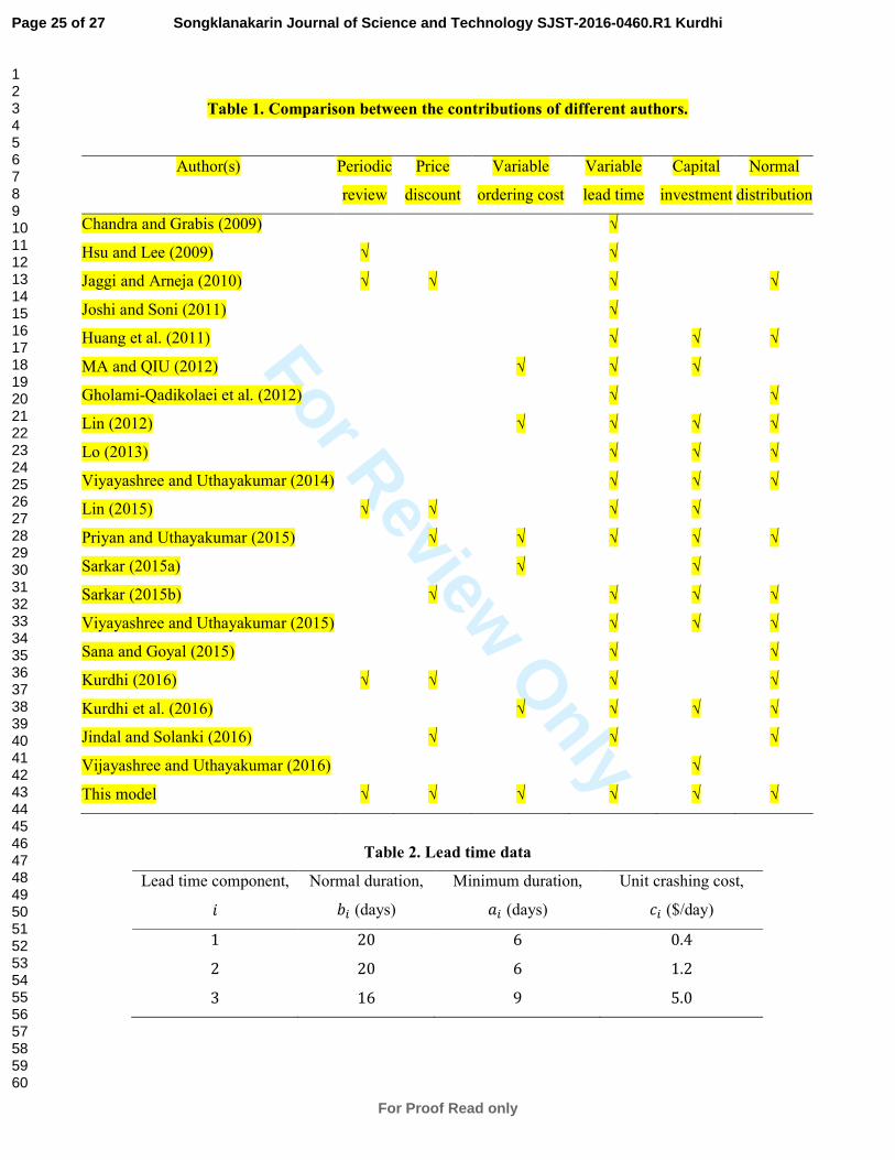
Table 1. Comparison between the contributions of different authors

The applications of the periodic inventory models can often be found in managing

inventory cases such as smaller retail stores, grocery stores and drugstores. For this, in

contrast to the continuous review inventory model, a periodic review model will be

investigated by considering backorder price discount, controllable lead time, and capital

investment to accommodate more practical feature of the real inventory system. In this

paper, the logarithmic function as investment cost functional form to analyze the effects

of increasing investment to reduce the ordering cost. Besides, the lead time can be

decomposed into several mutually independent components each having a different

crashing cost for shortening lead time. Moreover, there is an option in which while a

shortage occur, a price discount can always be offered on the stockout them to secure

more backorders. The protection interval demand follows a normal distribution.

Page 8 of 27

For Proof Read only

Songklanakarin Journal of Science and Technology SJST-2016-0460.R1 Kurdhi

123456789101112131415161718192021222324252627282930313233343536373839404142434445464748495051525354555657585960

For Review O

nly

6

Furthermore, a computational algorithm with the help of the software Mathematica 8 is

furnished to find the optimal values of the decision-making variables. Finally, some

numerical examples and sensitivity analysis are given to illustrate the solution

procedure of the proposed model and the effects of the parameters.

2. Notations and Assumptions

The following notations are used throughout the paper in order to develop the

mathematical model:

� : average demand (units per unit time)

�� : initial ordering cost per order

�(�) : capital investment required to achieve ordering cost �, 0 < � ≤ �0 ℎ : inventory holding cost per unit per unit time

� : target stock level

�� : upper bound of the backorder rate

� : backorder price discount offered by the supplier per unit

� : marginal profit (i.e. cost of lost demand) per unit

�(�) : total crashing cost of a cycle � : demand during the protection interval, � + �, which has a probability density function (p.d.f.) �� with finite mean �(� + �) and standard deviation �√� + � � : fractional opportunity cost of capital per year

�� : safety factor

� : stock-out probability

� : standard normal distribution

Φ : standard normal cumulative distribution function

Page 9 of 27

For Proof Read only

Songklanakarin Journal of Science and Technology SJST-2016-0460.R1 Kurdhi

123456789101112131415161718192021222324252627282930313233343536373839404142434445464748495051525354555657585960

For Review O

nly

7

�(⋅) : mathematical expectation

! : maximum value of and 0, i.e., ! = max{ , 0}. Decision variables

� : ordering cost per order

� : backorder rate, 0 < � < 1 � : length of a review period (unit time)

� : length of lead time (unit time)

In addition, the following assumptions are made.

1. The inventory level is reviewed every � units of time. A sufficient quantity is

ordered up to the target stock level �, and the ordering quantity is received after � units of time. The length of the lead time � does not exceed an inventory cycle time

� so that there is never more than a single order outstanding in any cycle.

2. The target stock level � = expected demand during the protection interval + safety

stock (**), and ** = �� ×(standard deviation of demand during protection interval

(� + �)), i.e., � = �(� + �) + ���√� + �, where ,(� > �) = �. 3. During the stock-out period, the backorder rate, �, is variable and is in proportion

to the price discount offered by the supplier per unit �. The backorder rate is defined as � = �� �/ �, where 0 ≤ �� < 1 and 0 ≤ � < �, �� is upper bound of the backorder rate, � is backorder price discount offered by the supplier per unit, and � is marginal profit per unit.

4. The lead time � can be decomposed into / mutually independent components, each

of which has a different crashing cost for reduce lead time. The 0-th component has

a normal duration 12, minimum duration 32, and crashing cost per unit time 42. For

Page 10 of 27

For Proof Read only

Songklanakarin Journal of Science and Technology SJST-2016-0460.R1 Kurdhi

123456789101112131415161718192021222324252627282930313233343536373839404142434445464748495051525354555657585960

For Review O

nly

8

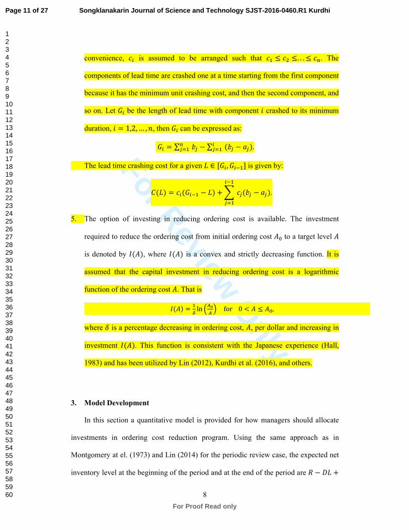
convenience, 42 is assumed to be arranged such that 45 ≤ 46 ≤. . . ≤ 48. The components of lead time are crashed one at a time starting from the first component

because it has the minimum unit crashing cost, and then the second component, and

so on. Let 92 be the length of lead time with component 0 crashed to its minimum

duration, 0 = 1,2, … , /, then 92 can be expressed as: 92 = ∑ 8>?5 1> − ∑ 2>?5 (1> − 3>).

The lead time crashing cost for a given � ∈ [92 , 92C5] is given by: �(�) = 42(92C5 − �) +E2C5

>?5 4>(1> − 3>). 5. The option of investing in reducing ordering cost is available. The investment

required to reduce the ordering cost from initial ordering cost �� to a target level � is denoted by �(�), where �(�) is a convex and strictly decreasing function. It is assumed that the capital investment in reducing ordering cost is a logarithmic

function of the ordering cost �. That is �(�) = 5F ln IJKJ L for0 < � ≤ ��,

where P is a percentage decreasing in ordering cost, �, per dollar and increasing in investment �(�). This function is consistent with the Japanese experience (Hall, 1983) and has been utilized by Lin (2012), Kurdhi et al. (2016), and others.

3. Model Development

In this section a quantitative model is provided for how managers should allocate

investments in ordering cost reduction program. Using the same approach as in

Montgomery at el. (1973) and Lin (2014) for the periodic review case, the expected net

inventory level at the beginning of the period and at the end of the period are � − �� +

Page 11 of 27

For Proof Read only

Songklanakarin Journal of Science and Technology SJST-2016-0460.R1 Kurdhi

123456789101112131415161718192021222324252627282930313233343536373839404142434445464748495051525354555657585960

For Review O

nly

9

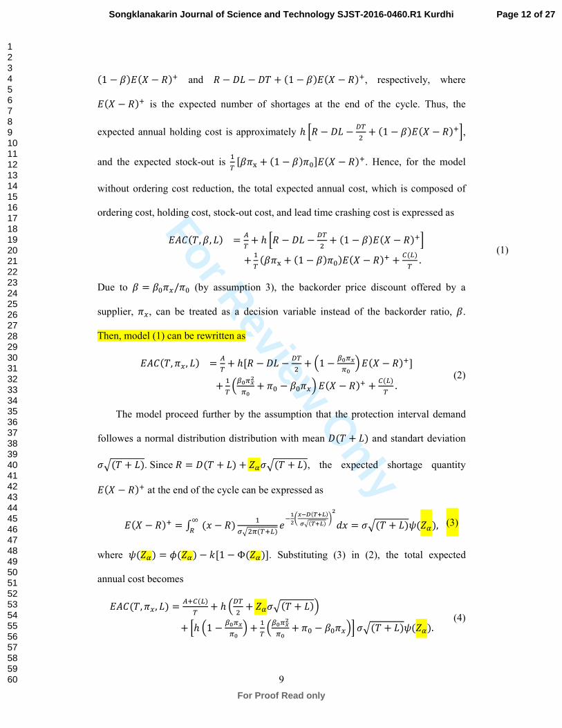
(1 − �)�(� − �)! and � − �� − �� + (1 − �)�(� − �)!, respectively, where

�(� − �)! is the expected number of shortages at the end of the cycle. Thus, the

expected annual holding cost is approximately ℎ Q� − �� − RS6 + (1 − �)�(� − �)!T, and the expected stock-out is

5S [� U + (1 − �) �]�(� − �)!. Hence, for the model

without ordering cost reduction, the total expected annual cost, which is composed of

ordering cost, holding cost, stock-out cost, and lead time crashing cost is expressed as

���(�, �, �) = JS + ℎ Q� − �� − RS6 + (1 − �)�(� − �)!T+ 5S (� U + (1 − �) �)�(� − �)! + V(W)S . (1)

Due to � = �� �/ � (by assumption 3), the backorder price discount offered by a

supplier, �, can be treated as a decision variable instead of the backorder ratio, �. Then, model (1) can be rewritten as

���(�, �, �) = JS + ℎ[� − �� − RS6 + I1 − XKYZYK L�(� − �)!]+ 5S IXKYZ[YK + � − �� �L �(� − �)! + V(W)S . (2)

The model proceed further by the assumption that the protection interval demand

followes a normal distribution distribution with mean �(� + �) and standart deviation �\(� + �). Since � = �(� + �) + ���\(� + �), the expected shortage quantity

�(� − �)! at the end of the cycle can be expressed as �(� − �)! = ] _̂ ( − �) 5`\6Y(S!W) aCb[cZde(fgh)i\(fgh) j[k = �\(� + �)l(��), (3)

where l(��) = �(��) − m[1 − Φ(��)]. Substituting (3) in (2), the total expected annual cost becomes

���(�, �, �) = J!V(W)S + ℎ IRS6 + ���\(� + �)L+ Qℎ I1 − XKYZYK L + 5S IXKYZ[YK + � − �� �LT �\(� + �)l(��). (4)

Page 12 of 27

For Proof Read only

Songklanakarin Journal of Science and Technology SJST-2016-0460.R1 Kurdhi

123456789101112131415161718192021222324252627282930313233343536373839404142434445464748495051525354555657585960

For Review O

nly

10

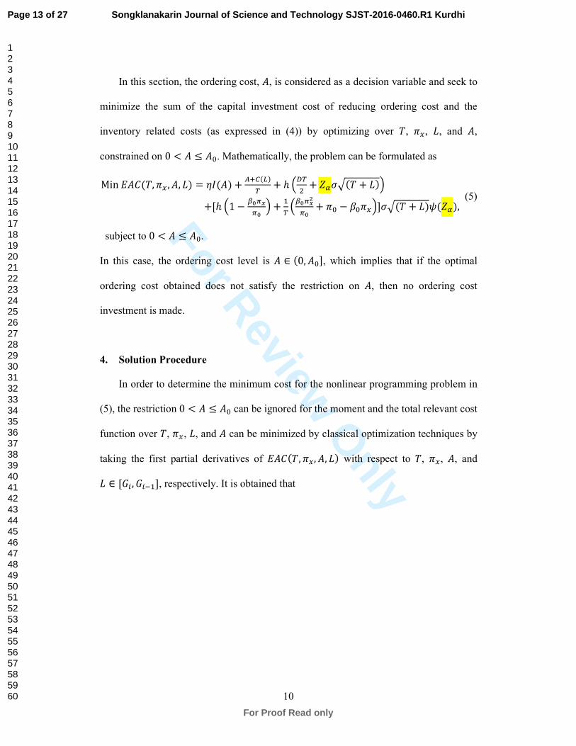
In this section, the ordering cost, �, is considered as a decision variable and seek to minimize the sum of the capital investment cost of reducing ordering cost and the

inventory related costs (as expressed in (4)) by optimizing over �, �, �, and �, constrained on 0 < � ≤ ��. Mathematically, the problem can be formulated as

Min���(�, � , �, �) = ��(�) + J!V(W)S + ℎ IRS6 + ���\(� + �)L+[ℎ I1 − XKYZYK L + 5S IXKYZ[YK + � − �� �L]�\(� + �)l(��), (5) subject to 0 < � ≤ ��. In this case, the ordering cost level is � ∈ (0, ��], which implies that if the optimal

ordering cost obtained does not satisfy the restriction on �, then no ordering cost investment is made.

4. Solution Procedure

In order to determine the minimum cost for the nonlinear programming problem in

(5), the restriction 0 < � ≤ �� can be ignored for the moment and the total relevant cost

function over �, �, �, and � can be minimized by classical optimization techniques by

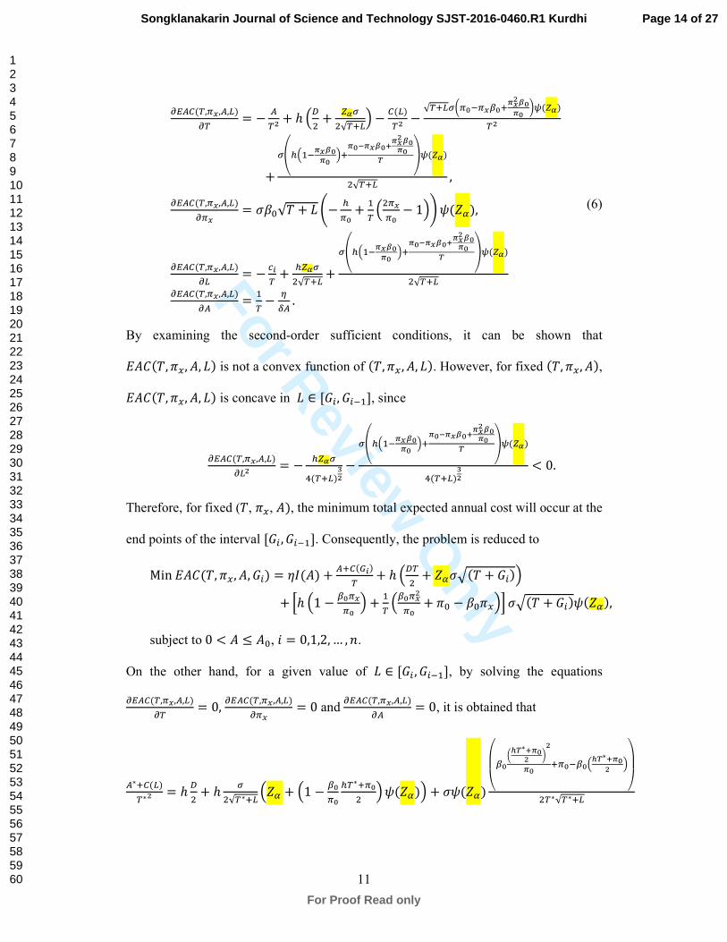
taking the first partial derivatives of ���(�, �, �, �) with respect to �, �, �, and � ∈ [92 , 92C5], respectively. It is obtained that

Page 13 of 27

For Proof Read only

Songklanakarin Journal of Science and Technology SJST-2016-0460.R1 Kurdhi

123456789101112131415161718192021222324252627282930313233343536373839404142434445464748495051525354555657585960

For Review O

nly

11

pqJV(S,YZ,J,W)pS = − JS[ + ℎ IR6 + rs`6√S!WL − V(W)S[ − √S!W`cYKCYZXK!tZ[uKtK jv(rs)S[

+ `wxI5CtZuKtK L!tKdtZuKgtZ[uKtKf yv(rs)6√S!W ,

pqJV(S,YZ,J,W)pYZ = ���√� + � z− xYK + 5S I6YZYK − 1L{l(��),pqJV(S,YZ,J,W)pW = − |}S + xrs`6√S!W +

`wxI5CtZuKtK L!tKdtZuKgtZ[uKtKf yv(rs)6√S!WpqJV(S,YZ,J,W)pJ = 5S − ~FJ .

(6)

By examining the second-order sufficient conditions, it can be shown that

���(�, �, �, �) is not a convex function of (�, � , �, �). However, for fixed (�, �, �), ���(�, �, �, �) is concave in � ∈ [92, 92C5], since pqJV(S,YZ,J,W)pW[ = − xrs`�(S!W)�[ −

`wxI5CtZuKtK L!tKdtZuKgtZ[uKtKf yv(rs)�(S!W)�[ < 0.

Therefore, for fixed (�, �, �), the minimum total expected annual cost will occur at the

end points of the interval [92 , 92C5]. Consequently, the problem is reduced to

Min���(�, �, �, 92) = ��(�) + J!V(�})S + ℎ IRS6 + ���\(� + 92)L+ Qℎ I1 − XKYZYK L + 5S IXKYZ[YK + � − �� �LT �\(� + 92)l(��),

subject to 0 < � ≤ ��, 0 = 0,1,2, … , /. On the other hand, for a given value of � ∈ [92 , 92C5], by solving the equations pqJV(S,YZ,J,W)pS = 0, pqJV(S,YZ,J,W)pYZ = 0 and pqJV(S,YZ,J,W)pJ = 0, it is obtained that

J∗!V(W)S∗[ = ℎ R6 + ℎ `6√S∗!W I�� + I1 − XKYK xS∗!YK6 Ll(��)L + �l(��)���XKc�f∗gtK[ j[tK !YKCXKI�f∗gtK[ L

���

6S∗√S∗!W

Page 14 of 27

For Proof Read only

Songklanakarin Journal of Science and Technology SJST-2016-0460.R1 Kurdhi

123456789101112131415161718192021222324252627282930313233343536373839404142434445464748495051525354555657585960

For Review O

nly

12

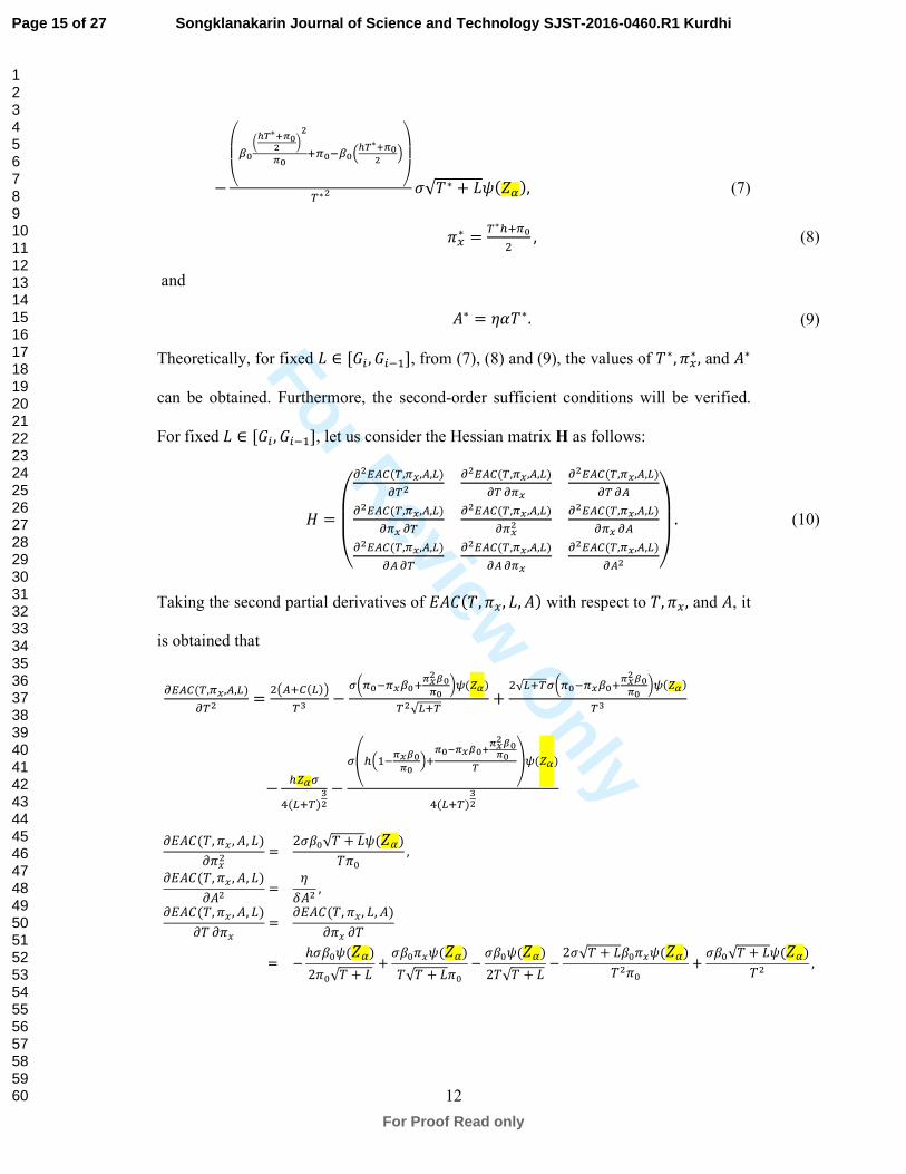
−���XKc�f∗gtK[ j[tK !YKCXKI�f∗gtK[ L

���

S∗[ �√�∗ + �l(��), (7) �∗ = S∗x!YK6 , (8)

and

�∗ = ���∗. (9)

Theoretically, for fixed � ∈ [92 , 92C5], from (7), (8) and (9), the values of �∗, �∗ , and �∗ can be obtained. Furthermore, the second-order sufficient conditions will be verified.

For fixed � ∈ [92 , 92C5], let us consider the Hessian matrix H as follows:

� =����p[qJV(S,YZ,J,W)pS[ p[qJV(S,YZ,J,W)pS pYZ p[qJV(S,YZ,J,W)pSpJp[qJV(S,YZ,J,W)pYZ pS p[qJV(S,YZ,J,W)pYZ[ p[qJV(S,YZ,J,W)pYZ pJp[qJV(S,YZ,J,W)pJpS p[qJV(S,YZ,J,W)pJpYZ p[qJV(S,YZ,J,W)pJ[ �

��� . (10)

Taking the second partial derivatives of ���(�, �, �, �) with respect to �, �, and �, it is obtained that

pqJV(S,YZ,J,W)pS[ = 6�J!V(W)�S� − `cYKCYZXK!tZ[uKtK jv(rs)S[√W!S + 6√W!S`cYKCYZXK!tZ[uKtK jv(rs)S�

− xrs`�(W!S)�[ −`wxI5CtZuKtK L!tKdtZuKgtZ[uKtKf yv(rs)

�(W!S)�[

∂���(�, � , �, �)∂ �6 = 2���√� + �l(��)� � ,∂���(�, � , �, �)∂�6 = �P�6 ,∂���(�, � , �, �)∂� ∂ � = ∂���(�, �, �, �)∂ � ∂�= − ℎ���l(��)2 �√� + � + ��� �l(��)�√� + � � − ���l(��)2�√� + � − 2�√� + ��� �l(��)�6 � + ���√� + �l(��)�6 ,

Page 15 of 27

For Proof Read only

Songklanakarin Journal of Science and Technology SJST-2016-0460.R1 Kurdhi

123456789101112131415161718192021222324252627282930313233343536373839404142434445464748495051525354555657585960

For Review O

nly

13

∂���(�, � , �, �)∂� ∂� = ∂���(�, �, �, �)∂� ∂� = − 1�6 ,∂���(�, � , �, �)∂ � ∂� = ∂���(�, �, �, �)∂� ∂ � = 0,

We proceed by evaluating the principal minor determinant of the Hessian matrix H at

point (�∗, �∗ , �∗). The first and second principal minor determinant of H then become

|�55| = 6(J!V(W))S� − [5� ℎ� z� + �)C�[ z�� + I1 − XKYZYK Ll(��){�− 5S[ (� + �)Cb[ I � − �� � + XKYZ[YK L�l(��) + 6S� (� + �)Cb[ I � − �� � + XKYZ[YK L �l(��)> J(�S!�W)6S�(S!W) + (S!�W)�YKCXKYZ!uKtZ[tK �`v(��)6S�√S!W > 0

and

|�66| = �p[qJV(S,YZ,J,W)pS[ p[qJV(S,YZ,J,W)pS pYZp[qJV(S,YZ,J,W)pYZ pS p[qJV(S,YZ,J,W)pYZ[�

= Q(S!W)XK`[v[(rs)S�YK[ T Q �6(1 − ��) + I�XKxS6 + �XKYK6 L I � − Sx6 − YK6 LT = Q(S!W)XK`[v[(rs)S�YK[ T [ �6(1 − ��) + 3�� �( � − �)] > 0.

Next, the third principal minor determinant of H is

|���| = ��p[qJV(S,YZ,J,W)pS[ p[qJV(S,YZ,J,W)pS pYZ p[qJV(S,YZ,J,W)pS pJp[qJV(S,YZ,J,W)pYZ pS p[qJV(S,YZ,J,W)pYZ[ p[qJV(S,YZ,J,W)pYZ pJp[qJV(S,YZ,J,W)pJpS p[qJV(S,YZ,J,W)pJpYZ p[qJV(S,YZ,J,W)pJ[

��

= ~�J[ I(S!W)XK`[v[(rs)S�YK[ L [ �6(4 − ��) − 3��(ℎ�)6] − I6XK`√S!Wv(rs)SYK L I− 5S[L6= ~�J[ I(S!W)XK`[v[(rs)S�YK[ L [ �6(4 − ��) − 3��(ℎ�)6] − I6XK`√S!Wv(rs)S�YK L.

It is difficult to determine mathematically the sign of |���|. However, since |�55| and |�66| are all positive, then (�∗, �∗ , �∗) are the optimal solution if |���| > 0. Furthermore, it is not possible to determine the closed-form solution for (�∗, �∗ , �∗)

from (7), (8) and (9). However, the optimal value of (�∗, �∗ , �∗) can be obtained by

Page 16 of 27

For Proof Read only

Songklanakarin Journal of Science and Technology SJST-2016-0460.R1 Kurdhi

123456789101112131415161718192021222324252627282930313233343536373839404142434445464748495051525354555657585960

For Review O

nly

14

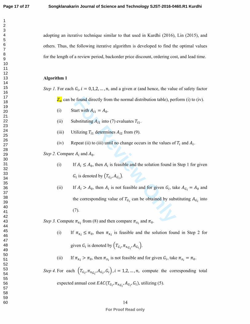
adopting an iterative technique similar to that used in Kurdhi (2016), Lin (2015), and

others. Thus, the following iterative algorithm is developed to find the optimal values

for the length of a review period, backorder price discount, ordering cost, and lead time.

Algorithm 1

Step 1. For each 92 , 0 = 0,1,2,… , /, and a given � (and hence, the value of safety factor �� can be found directly from the normal distribution table), perform (i) to (iv).

(i) Start with �25 = ��. (ii) Substituting �25 into (7) evaluates �25. (iii) Utilizing �25 determines �26 from (9).

(iv) Repeat (ii) to (iii) until no change occurs in the values of �2 and �2. Step 2. Compare �2 and ��.

(i) If �2 ≤ ��, then �2 is feasible and the solution found in Step 1 for given 92 is denoted by ���} , ��}�.

(ii) If �2 > ��, then �2 is not feasible and for given 92, take ��} = �� and the corresponding value of ��} can be obtained by substituting ��} into (7).

Step 3. Compute U2 from (8) and then compare �} and �. (i) If U2 ≤ �, then U2 is feasible and the solution found in Step 2 for

given 92 is denoted by I��} , U�} , ��}L. (ii) If U2 > �, then �} is not feasible and for given 92, take �} = �.

Step 4. For each I��} , U�} , ��} , 92L , 0 = 1,2, … , /, compute the corresponding total

expected annual cost ���(��} , U�} , ��} , 92), utilizing (5).

Page 17 of 27

For Proof Read only

Songklanakarin Journal of Science and Technology SJST-2016-0460.R1 Kurdhi

123456789101112131415161718192021222324252627282930313233343536373839404142434445464748495051525354555657585960

For Review O

nly

15

Step 5. Find min2?5,6,…,8 ���(��} , U�} , ��}, 92). If EAC(�� , ��, ��, ��)=min2?5,6,…,8 ���(��} , U�} , ��} , 92), then

��� , ��, ��, ��� is the optimal solution.

Note that, once (��, ��, ��, ��) is obtained, the optimal target level �� = �(�� + ��) +m�\�� + �� and the optimal backorder rate �� = �� ��/ � follow.

5. Numerical Example

The numerical examples given below illustrate the above solution procedure.

Consider a periodic review inventory system with the following data: D = 600

units/year, �� = $200/order, ℎ = $20/unit/year, �= $150/unit, � = 7 units/week, and the lead time has three components with data shown in Table 2.

Table 2. Lead time data

Suppose that the protection interval demands follows a normal distribution.

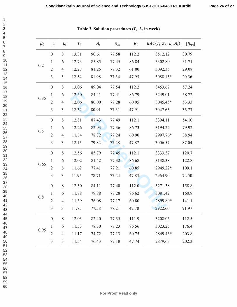
Consider the cases when the upper bounds of the backorder rate �� = 0.2, 0.35, 0.5, 0.65, 0.8 and 0.95, and � = 0.2 (in this situation, the value of safety factor, ��, can be found directly from the standard normal distribution table and is 0.845). Applying the

proposed algorithm procedure yields the results shown in Table 3. From this table, the

optimal inventory policy can easily be found by comparing ���(�2 , �0 , �2, 92), for 0 = 0, 1, 2, 3, and these are summarized in Table 4. Moreover, the optimal results of the

fixed ordering cost model are listed in the same table to illustrate the effects of investing

in ordering cost reduction. From Table 4, it can be observed that increasing the value of

upper bound of the backorder rate will results in a decrease in the review period, the

Page 18 of 27

For Proof Read only

Songklanakarin Journal of Science and Technology SJST-2016-0460.R1 Kurdhi

123456789101112131415161718192021222324252627282930313233343536373839404142434445464748495051525354555657585960

For Review O

nly

16

backorder price discount, ordering cost, and the total expected annual cost. Furthermore,

comparing our model with that of the fixed ordering cost case, it can be observed that

the savings range from 34.81% to 34.93%, which shows that significant savings can be

achieved due to controlling the ordering cost.

Table 3. Solution procedures (��, �� in week)

Table 4. Summary of the optimal solutions

In addition, the effects of changes in the system parameters ℎ, �, and � on the optimal review period, backorder price discount, lead time, ordering cost, and minimum

total expected annual cost, will be examined. Using the same data and assumptions, �� is fixed at 0.95 and a sensitivity analysis is performed by changing each of the

parameters by +50%, +25%, -25%, and -50%, taking one parameter at a time and

keeping the remaining parameters unchanged. The results are shown in Table 5. On the

basis of the results of the Table 5, the following observations can be made.

(1) �� and �� decrease while �� and EAC(��, ��, ��, ��) increase with an increase in the value of the holding cost parameter, ℎ. Besides, it can be observed that as the value ℎ changes, the value �� is not influenced.

(2) ��, �� and �� decrease, whereas EAC(�� , ��, �� , ��) increases with an increase in the value of the demand parameter, �. Besides, the value �� is not influenced by changes in the value of �.

(3) ��, ��, ��, and EAC(�� , ��, ��, ��) increase while �� decreases with an increase in the value of the model parameter �.

Page 19 of 27

For Proof Read only

Songklanakarin Journal of Science and Technology SJST-2016-0460.R1 Kurdhi

123456789101112131415161718192021222324252627282930313233343536373839404142434445464748495051525354555657585960

For Review O

nly

17

Table 5. Effects of change in the parameters

6. Conclusions

The purpose of this paper is to investigate a mixture inventory policy on a

controlling ordering cost in the stochastic periodic review involving controllable

backorder price discount and variable lead time for protection interval demand with

normal distribution. By analyzing the total expected annual cost, an algorithm is

developed to determine the optimal review period, backorder price discount, ordering

cost, and lead time so that the total expected annual cost incurred has the minimum

value. The results of the numerical examples indicate that by making decisions with

capital investment in reducing ordering cost, it would help to lower the system cost, and

a significant amount of savings can be obtained. To understand the effects of the

optimal solution on changes in the value of the different parameters associated with the

inventory system, sensitivity analysis is performed. Furthermore, it can be observed

from the sensitivity analysis that the total expected annual cost are more highly sensitive

to the changes in the value of holding cost parameter,ℎ, than to the changes in � and �. This paper is limited in the known demand distribution. In real situations, we often get

difficulty in providing a precise estimation on the probability density function due to the

insufficiency of historical data. Therefore, for further consideration on this problem, it

would be interested to propose a distribution-free model according to the mean and the

standard deviation of demand. Moreover, we can deal with a mixed stochastic inventory

model that the stock-out term in the objective function is replaced by a service level

constraint. Another possible direction may be conducted by considering stochastic

Page 20 of 27

For Proof Read only

Songklanakarin Journal of Science and Technology SJST-2016-0460.R1 Kurdhi

123456789101112131415161718192021222324252627282930313233343536373839404142434445464748495051525354555657585960

For Review O

nly

18

periodic review inventory models with controllable safety factor or incorporating the

defective items and inspection errors in the future extension of the present article.

Acknowledgement

The authors would like to express their appreciation to the PNBP Sebelas Maret

University, Indonesia, for their financial support.

References

Bhowmick, J. and Samanta, G.P. 2012. Optimal inventory policies for imperfect

inventory wth price dependent stochastic demand and partially backlogged

shortages. Yugoslav Journal of Operations Research. 22, 199-223.

Chandra, C. and Grabis, J. 2008. Inventory management with variable lead-time

dependent procurement cost. Omega. 36(5), 877-887.

Gholami-Qadikolaei, A., Mohammadi, M., Amanpour-Bonab, S. and Mirzazadeh A.

2012. A continuous review inventory system with controllable lead time and

defective items in partial and perfect lead time demand distribution information

environments. Journal International Journal of Management Science and

Engineering Management. 7(3), 205-212.

Hall, R.W. 1983. Zero inventories. Dow Jones-Irwin, Homewood, Ill, USA.

Huang, C.K., Cheng, T.L., Kao, T.C. and Goyal, S.K. 2011. An integrated inventory

model involving manufacturing setup cost reduction in compound Poisson

process. International Journal of Production Research. 49(4), 1219-1228.

Hsu, S.L. and Lee, C.C. 2009. Replenishment and lead time decisions in manufacturer

retailer chains. Transportation Research Part E. 45, 398-408.

Page 21 of 27

For Proof Read only

Songklanakarin Journal of Science and Technology SJST-2016-0460.R1 Kurdhi

123456789101112131415161718192021222324252627282930313233343536373839404142434445464748495051525354555657585960

For Review O

nly

19

Jaggi, C.K. and Arneja, N. 2010. Periodic inventory model with unstable lead-time and

setup cost with backorder discount. International Journal of Applied Decision

Sciences. 3(1), 53-73.

Jindal, P. and Solanki, A. 2016. Integrated supply chain inventory model with quality

improvement involving controllable lead time and backorder price discount.

International Journal of Industrial Engineering Computations. 7, 463-480.

Joshi, M. and Soni, H. 2011. (Q, R) inventory model with service level constaint and

variable lead time in fuzzy-stochastic environment. International Journal of

Industrial Engineering Computations. 2, 901-912.

Kurdhi, N.A. 2016. Lead time and ordering cost reductions are interdependent in

periodic review integrated inventory model with backorder price discount. Far

East Journal of Mathematical Sciences. 100(6), 821-976.

Kurdhi, N.A., Sutanto, Kristanti, Prasetyawati, M.V.A. and Lestari, S.M.P. 2016.

Continuous review inventory models under service level constraint with

probabilistic fuzzy number during uncertain received quantity. International

Journal of Services and Operations Management. 23(4), 443-466.

Lin, H-J. 2015. A stochastic periodic review inventory model with back-order discounts

and ordering cost dependent on lead time for the mixtures of distributions. TOP.

23(2), 386-400.

Lin, Y.J. 2012. Effective investment to reduce setup cost in a mixture inventory model

involving controllable backorder rate and variable lead time with a service level

constraint. Mathematical Problems in Engineering, 2012, Article ID 689061, 15

pages.

Page 22 of 27

For Proof Read only

Songklanakarin Journal of Science and Technology SJST-2016-0460.R1 Kurdhi

123456789101112131415161718192021222324252627282930313233343536373839404142434445464748495051525354555657585960

For Review O

nly

20

Lo, C. 2013. A collaborative business model for imperfect process with setup cost and

lead time reductions. Open Journal of Social Sciences. 1, 6-11.

MA, W-M. and QIU, B-B. 2012. Distribution free continuous review inventory model

with controllable lead time and setup cost in the presence of a service level

constraint. Mathematical Problems in Engineering. 2012, Article ID 867847, 16

pages.

Montgomery, D.C., Bazaraa, M.S. and Keswani, A.K. 1973. Inventory models with a

mixture of backorders and lost sales. Nav Res Logist. 20, 255–263.

Pan, J.C-H. and Hsiao, Y-C. 2005. Integrated inventory models with controllable lead

time and backorder discount considerations. International Journal of Production

Economics. 93-94, 387-397.

Porteus, E.L. 1985. Investing in reduction setups in the EOQ model. Management

Science. 31(8), 998–1010.

Priyan, S. and Uthayakumar, R. 2015. Continuous review inventory model with

controllable lead time, lost sales rate and order processing cost when the received

quantity is uncertain. Journal of Manufacturing Systems. 34, 23-33.

Sana, S.S. and Goyal, S.K. 2015. (Q, r, L) model for stochastic demand with lead-time

dependent partial backlogging. Annals of Operations Research. 233(1), 401-410.

Sarkar, B., Chaudhuri, K. and Moon, I. 2015a. Manufacturing setup cost reduction and

quality improvement for the distribution free continuous-review inventory model

with a service level constraint. Journal of Manufacturing Systems. 34, 74–82.

Sarkar, B., Mandal, B. and Sarkar, S. 2015b. Quality improvement and backorder price

discount under controllable lead time in an inventory model. Journal of

Manufacturing Systems. 35, 26-36.

Page 23 of 27

For Proof Read only

Songklanakarin Journal of Science and Technology SJST-2016-0460.R1 Kurdhi

123456789101112131415161718192021222324252627282930313233343536373839404142434445464748495051525354555657585960

For Review O

nly

21

Tersine, R.J. 1982. Principles of inventory and materials management. Nort Holland,

New York.

Tersine, R.J. and Hummingbird, E. 1995. A lead-time reduction the search for

competitive advantage. International Journal of Operations and Production

Management. 15, 8-18.

Vijayashree, M. and Uthayakumar, R. 2014. An integrated inventory model with

controllable lead time and setup cost reduction for defective and non-defective

items. International Journal of Supply and Operations Management. 1(2), 190-

215.

Vijayashree, M. and Uthayakumar, R. 2015. Integrated inventory model with

controllable lead time involving investment for quality improvement in supply

chain system. International Journal of Supply and Operations Management. 2(1),

617-639.

Vijayashree, M. and Uthayakumar, R. 2016. An integrated vendor and buyer inventory

model with investment for quality improvement and setup cost reduction.

Operations Research and Application: An International Journal. 3(2), 1-14.

Yang, M.F., Lin, Y., Ho, L.H. and Kao, W.F. 2016. An integrated multiechelon logistics

model with uncertain delivery lead time and quality unreliability. Mathematical

Problems in Engineering. 2016, Article ID 8494268, 13 pages.

Page 24 of 27

For Proof Read only

Songklanakarin Journal of Science and Technology SJST-2016-0460.R1 Kurdhi

123456789101112131415161718192021222324252627282930313233343536373839404142434445464748495051525354555657585960

For Review O

nly

Table 1. Comparison between the contributions of different authors.

Author(s) Periodic

review

Price

discount

Variable

ordering cost

Variable

lead time

Capital

investment

Normal

distribution

Chandra and Grabis (2009)

Hsu and Lee (2009)

Jaggi and Arneja (2010)

Joshi and Soni (2011)

Huang et al. (2011)

MA and QIU (2012)

Gholami-Qadikolaei et al. (2012)

Lin (2012)

Lo (2013)

Viyayashree and Uthayakumar (2014)

Lin (2015)

Priyan and Uthayakumar (2015)

Sarkar (2015a)

Sarkar (2015b)

Viyayashree and Uthayakumar (2015)

Sana and Goyal (2015)

Kurdhi (2016)

Kurdhi et al. (2016)

Jindal and Solanki (2016)

Vijayashree and Uthayakumar (2016)

This model

√

√

√

√

√

√

√

√

√

√

√

√

√

√

√

√

√

√

√

√

√

√

√

√

√

√

√

√

√

√

√

√

√

√

√

√

√

√

√

√

√

√

√

√

√

√

√

√

√

√

√

√

√

√

√

√

√

√

√

√

√

√

√

√

Table 2. Lead time data

Lead time component,

�

Normal duration,

�� (days)

Minimum duration,

�� (days)

Unit crashing cost,

�� ($/day)

1

2

3

20

20

16

6

6

9

0.4

1.2

5.0

Page 25 of 27

For Proof Read only

Songklanakarin Journal of Science and Technology SJST-2016-0460.R1 Kurdhi

123456789101112131415161718192021222324252627282930313233343536373839404142434445464748495051525354555657585960

For Review O

nly

Table 3. Solution procedures (��, �� in week)

�� � �� �� �� ��� �� ���(�� , ���

, �� , ��) |!""|

0.2

0

1

2

3

8

6

4

3

13.31

12.73

12.27

12.54

90.61

85.85

81.25

81.98

77.58

77.45

77.32

77.34

112.2

86.84

61.00

47.95

3512.12

3302.80

3092.35

3088.15*

30.79

31.71

29.08

20.36

0.35

0

1

2

3

8

6

4

3

13.06

12.50

12.06

12.34

89.04

84.41

80.00

80.91

77.54

77.41

77.28

77.31

112.2

86.79

60.95

47.91

3453.67

3249.01

3045.45*

3047.65

57.24

58.72

53.33

36.73

0.5

0

1

2

3

8

6

4

3

12.81

12.26

11.84

12.15

87.43

82.93

78.72

79.82

77.49

77.36

77.24

77.28

112.1

86.73

60.90

47.87

3394.11

3194.22

2997.76*

3006.57

54.10

79.92

88.94

87.04

0.65

0

1

2

3

8

6

8

3

12.56

12.02

11.62

11.95

85.79

81.42

77.41

78.71

77.45

77.32

77.21

77.24

112.1

86.68

60.85

47.83

3333.37

3138.38

2949.22*

2964.90

120.7

122.8

109.1

72.50

0.8

0

1

2

3

8

6

4

3

12.30

11.78

11.39

11.75

84.11

79.88

76.08

77.58

77.40

77.28

77.17

77.21

112.0

86.62

60.80

47.78

3271.38

3081.42

2899.80*

2922.60

158.8

160.9

141.1

91.97

0.95

0

1

2

3

8

6

4

3

12.03

11.53

11.17

11.54

82.40

78.30

74.72

76.43

77.35

77.23

77.13

77.18

111.9

86.56

60.75

47.74

3208.05

3023.25

2849.43*

2879.63

112.5

176.4

203.8

202.3

Page 26 of 27

For Proof Read only

Songklanakarin Journal of Science and Technology SJST-2016-0460.R1 Kurdhi

123456789101112131415161718192021222324252627282930313233343536373839404142434445464748495051525354555657585960

For Review O

nly

Table 4. Summary of the optimal solutions

Ordering cost reduction model Fixed ordering cost model (� = 200)

�� �$ �$ ��$ �$ �$ ���(∙) ���(∙) Savings (%)

0.20

0.35

0.50

0.65

0.80

0.95

3

4

4

4

4

4

12.54

12.06

11.84

11.62

11.39

11.17

77.34

77.28

77.24

77.21

77.17

77.13

81.98

80.00

78.72

77.41

76.08

74.72

47.95

60.95

60.90

60.85

60.80

60.75

3088.15

3045.45

2997.76

2949.22

2899.80

2849.43

4746.27

4672.85

4598.94

4524.55

4449.66

4374.24

34.93

34.82

34.81

34.81

34.83

34.85

Table 5. Effects of change in the parameters

Parameters’

value

% of change Optimum value

(�$, ��$, �$, �$)

EAC

(�$, ��$, �$, �$)

Percentage of

influence

ℎ=30

25

20

15

10

+50

+25

0

-25

-50

(8.68, 77.54, 4, 59.27)

(9.71, 77.35, 4, 65.73)

(11.17, 77.13, 4, 74.73)

(13.41, 76.89, 4, 88.41)

(17.49, 76.61, 4, 112.77)

3464.53

3169.05

2849.43

2496.10

2090.73

+17.75%

+10.09%

0%

-14.15%

-36.29%

)=900

750

600

450

300

+50

+25

0

-25

-50

(8.90, 76.69, 4, 59.33)

(9.85, 76.88, 4, 65.77)

(11.17, 77.14, 4, 74.73)

(13.13, 77.52, 4, 88.33)

(16.50, 78.21, 4, 112.44)

3335.95

3104.65

2849.43

2560.85

2220.94

+14.58%

+8.22%

0%

-11.27%

-28.30%

*=10.5

8.75

7

5.25

3.5

+50

+25

0

-25

-50

(13.15, 77.49, 3, 87.20)

(12.38, 77.34, 3, 82.03)

(11.17, 77.14, 4, 74.73)

(10.08, 76.92, 4, 67.36)

(8.81, 76.68, 4, 58.86)

3380.95

3137.28

2849.43

2524.05

2160.50

+15.72%

+9.17%

0%

-12.89%

-31.89%

Page 27 of 27

For Proof Read only

Songklanakarin Journal of Science and Technology SJST-2016-0460.R1 Kurdhi

123456789101112131415161718192021222324252627282930313233343536373839404142434445464748495051525354555657585960