for review only - home - dept. of statistics, texas a&m ...debdeep/papers/fm_radio.pdfvery long...
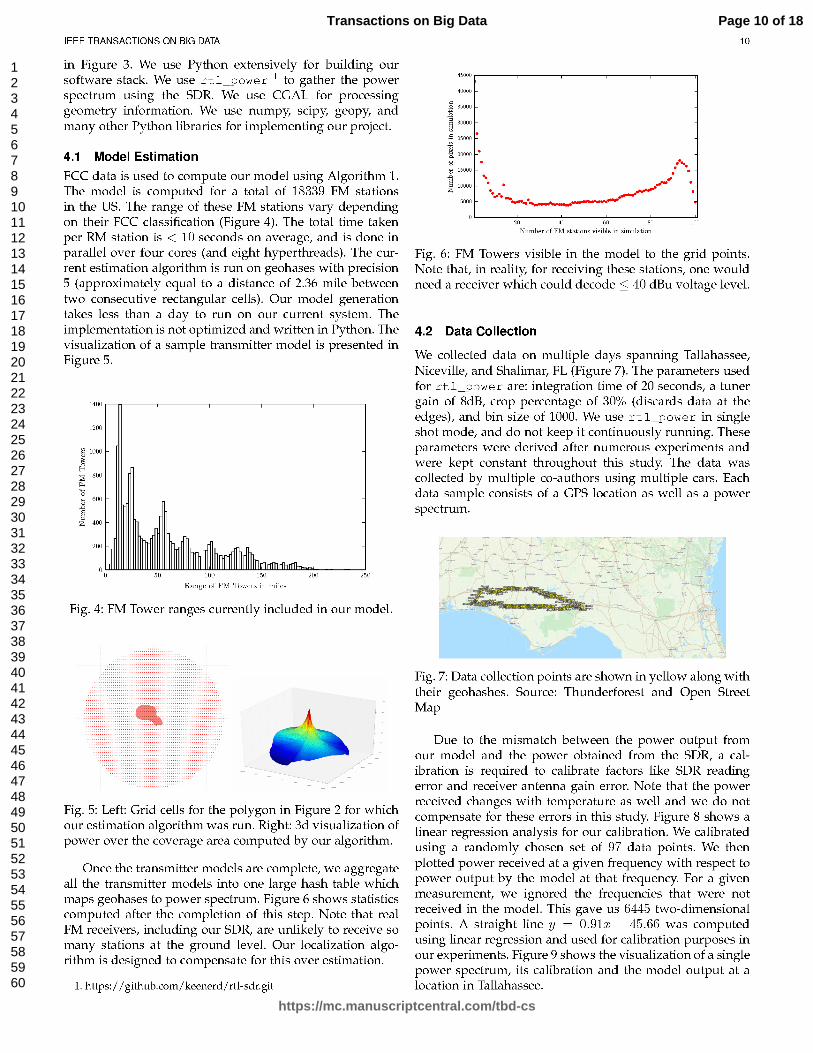
TRANSCRIPT

For Review O
nly
Large Scale FM Signal Strength Map Estimation For Passive
Approximate Localization
Journal: Transactions on Big Data
Manuscript ID Draft
Manuscript Types: Regular Paper
Keywords: Data Mining, Pattern Analysis, Large Scale Localization, Bayesian Decision Theory
https://mc.manuscriptcentral.com/tbd-cs
Transactions on Big Data

For Review O
nly
IEEE TRANSACTIONS ON BIG DATA 1
Large Scale FM Signal Strength Map EstimationFor Passive Approximate Localization
Piyush Kumar, President, CompGeom Inc, Tathagata Mukherjee, AFRL, MMO Institute,
Eduardo Pasiliao, AFRL, Munitions Directorate, Debdeep Pati, Assistant Professor, Florida State
University, and Liqin Xu, Technical Staff, CompGeom Inc.
Abstract—In this paper, we present a coarse, passive localization system for GPS denied environments. Our system is based on
broadcast FM radio signals and uses RSSI obtained using an inexpensive software defined radio (SDR).The RSSI thus obtained is
used for matching into a large database of estimated FM spectrum for the entire United States. We show that with an inexpensive
hardware for data acquisition and associated algorithms, we are capable of localizations that can be used for countering GPS spoofing.
The algorithm is based on a large-scale pre-processing phase that estimates the probable FM power spectrum in small rectangular
cells (realized using geohashes) across entire US, from various FM towers in the locality. The query phase first runs a peak detector on
the power spectrum obtained using the SDR and then solves a subset query problem to compute proposed locations (geohashes) to
be analyzed. Finally, it uses a simple Euclidean nearest neighbor search to localize the observed power spectrum to a location of
interest. We use more than nine hundred observed power spectra distributed over four hundred miles in Florida for experimentally
validating our query algorithm. We also provide a Bayesian decision theoretic explanation for the nearest neighbor search.
Index Terms—Big Data, Data Mining, Pattern Analysis, Machine Learning, Large Scale Localization, Nearest Neighbor Search,
Bayesian Decision Theory
✦
1 INTRODUCTION
GPS and its applications have become an integral part ofour daily lives. In spite of advances in the technology,
there are situations where GPS [1] becomes unreliable, isdenied, or is unavailable altogether [2], [3]. Land vehiclesare especially prone to accidental or deliberate GPS inter-ference [4], [5]. The ultimate outdoor localization systemshould not only localize in the absence of GPS but shouldalso provide a way to localize in case GPS is spoofed.Moreover such systems should easily scale to very largeareas, like entire countries, and should be easy to massproduce. This paper is a step in that direction.
Apart from GPS, many other Radio frequency (RF)based localization techniques have been proposed. Theseinclude beacon based or anchor based approaches [6], [7],[8], [9], [10], Time of Arrival (TOA) [11], Time Differenceof Arrival (TDoA) [12], and Angle of Arrival [10]. Mostof these approaches either need more complex and hencemore expensive hardware for prototyping, a complex timesynchronization step, a directional antenna or multiple an-tennas, or have problems with multipath.
In addition to the methods discussed above, there aresome distance-dependent features of the RF signal, for ex-ample Received Signal Strength Indicator (RSSI) [13], Signal-
• Piyush Kumar is currently with CompGeom Inc., Tallahassee FLE-mail: [email protected]
• Tathagata Mukherjee is currently with AFRL MMO InstituteE-mail: [email protected]
• Eduardo Pasiliao is currently a Senior Research Engineer with AFRLE-mail: [email protected]
• Debdeep Pati is currently with Statistics Department at FSUE-mail: [email protected]
• Liqin Xu: [email protected]• Authors contributed equally and sorted by last name
to-Noise Ratio (SNR) and Stereo Channel Separation (SCS),which have also been used for localization in GPS-freeenvironments [14]. RSSI based methods are usually easy toimplement, since it can be read directly from the hardware,and the computation complexity is low. However, methodsbased on RSSI usually do not scale very well and mayrequire very accurate timing measurements for synchro-nization. Moreover, the SNR and SCS based methods haverelatively high computational complexity and also requireengineering of the decoding process, so that the transmittedinformation can be used for localization [7]. As a result, weuse a method based on observed RSSI at the receiver in away that can be scaled to very large areas, like the entireUnited States.
Motivated by the success of FM based indoor localiza-tion techniques [7], we use FM broadcast radio signals forlarge scale outdoor localization in the absence of GPS. FMuses frequency modulation to provide high-fidelity soundover broadcast radio. The FM broadcast band falls between88MHz to 108MHz in the US with a 200kHz bandwidth. FMwaves are very high frequency (VHF) and hence are lesssensitive to weather conditions and terrain [7], [15], coversvery long distances and hence can be used for both indoorand outdoor localization when GPS is unavailable. More-over, as our method is based on RSSI within the constrain ofhardware costs, which is less than $25, it immediately rulesout the methods based on TOA, TDoA and AOA.
Our objective is to come up with a simple and fastalgorithm that can localize within a very large area inthe absence of GPS. Our method contains a pre-processingestimation phase and a query phase for localization. Inthe pre-processing phase, we compute an estimate of thepower spectrum at each point of our region of interest,
Page 1 of 18
https://mc.manuscriptcentral.com/tbd-cs
Transactions on Big Data
123456789101112131415161718192021222324252627282930313233343536373839404142434445464748495051525354555657585960

For Review O
nly
Page 2 of 18
https://mc.manuscriptcentral.com/tbd-cs
Transactions on Big Data
123456789101112131415161718192021222324252627282930313233343536373839404142434445464748495051525354555657585960
For Review O
nly
IEEE TRANSACTIONS ON BIG DATA 3
second approach achieves its objective without any commu-nication with a Global Positioning System. Traditional GPSbased localization [1] uses GPS receivers to communicatewith GPS satellites. The received data is used to computethe distance of the object from at least four known GPSsatellites. This is done using the idea of time of arrival(TOA) [11]. Once this computation is done, the final positionis computed using trilateration. GPS based systems sufferfrom several limitations, namely, lack of precision [18],jamming [5], disruption and spoofing [19].
In order to get around these problems people havesuggested the idea of assisted GPS [20]. In assisted GPS (A-GPS), there is a dedicated A-GPS server that also commu-nicates with the GPS receiver. The data from the server isused to augment the data received by the GPS receiver. Leeat al. [21] used the idea of radio-frequency assisted GPS (RF-GPS). RF-GPS uses differential GPS (DGPS) [22] in order tocorrect the errors and improve the accuracy of GPS.
More recently, work has been done in order to achievecentimeter level accuracy with GPS [23], [24]. Most of thecentimeter accurate GPS systems use the idea of carrierphase differential. Carrier phase differential uses the GPScarrier signal. This signal has much higher frequency andhence can be used to determine the distances to the satellitesmore accurately [25], [26], [27].
Apart from GPS based localization methods, there areabsolute positioning techniques that do not depend onGPS. These methods are usually called GPS-free localizationtechniques. One of the most common forms of GPS freepositioning is called Network based Geolocation [20], [28], [29].These methods are almost exclusively based on technologiesthat depend on wireless networks and use signal processingheavily. They use methods such as time of arrival, timedifference of arrival, angle of arrival, timing advance andmultipath fingerprinting [10], [11], [13], [30], [31], [32].
McEllroy et al. [33] developed a GPS free navigationsystem using the AM transmission band with the TDoAmethod. The idea is to use an AM tower with knownlocation and one reference receiver to estimate the secondreceiver’s location. In theory, this work can be extended touse FM Stations. This approach has an accuracy of 20m,but it relies on a known position of the reference receiver.Therefore, in a large area, it mandates the deployment ofa large number of reference receivers in order to performthe localization. More recently, ground based terrestrialtransmitters have been used to create a terrestrial versionof GPS, that does not depend on transmissions from GPSconstellations. One such system is called Locata [34]. Theyhave pioneered the use of ground based transmitters thatcan be used as an alternative to GPS satellites. One of themajor drawbacks of such a system is the need to invest inthe creation of a large network of Locata transmitters acrossthe world.
In order to implement a network based geolocationsystem, without the need for special transmitters, one canuse ambient radio signals. A straightforward approach tobuilding such a system is through the use of a finger-print database. Such systems are broadly categorized asfingerprint based localization system. The fingerprints canbe received signal strengths for Wifi based localization orFM based localization [35], [36]. They can also be readings
obtained from inertial sensors, in case, such readings haveunique characteristics at given locations [37]. This methodhas been extensively used for building indoor localizationsystems [9], [36], [37], [38]. The system scans the fingerprintat a given location of interest and then compares it with adatabase, which contains the fingerprints for every possiblelocation within the area of interest. The location of the pointof interest is determined based on a match found in thisdatabase.
Laoudias et al. [39] built such a system using smart-phones. Smartphones are used to collect data on Wifi accesspoints (APs) and create a database for the entire regionof interest. This collection is done offline. Finally, in thequery phase, the location of a point is determined by usingan Euclidean nearest neighbor search, on the database, inthe space of the RSSI values. A crowdsourced version ofa similar system was implemented by Petrou et al. [40].Adding another dimension to localization, Konstantinidiset al. have studied privacy preserving indoor localizationusing smartphones [41].
Fang et.al. [8] did an extensive study on FM finger-print based localization in a small area, for studying thepossibility of meeting the FCC requirement [42] (50 meterserror for 67 percent of calls for handset-based devices).They implemented a fingerprint based localization systemusing the RSSI values of the FM signals as the fingerprints.First they created the fingerprint database using a spectrumanalyzer. Then they used the idea of correlation to comparethe obtained signal at a point with those stored in thedatabase. They also compared the results obtained fromFM and GSM signals as the sources. It is difficult, if notimpossible, to extend these results to an entire countrylike the United States because of the large amount of datacollection required.
Abdelnasser et al. [37] implemented a system with fin-gerprints from several sensors on a mobile phone. They no-ticed that different indoor locations have unique signatureson one or more sensors that are available on a cell phone.For example, stairs have very different signature in the ac-celerometer as compared to level floor. Such locations, withunique signatures are called landmarks. Their system usesthese landmarks and combines them with dead-reckoningfor indoor localization.
Azizyan et al. [43] used a novel technique called Sur-roundSense to logically localize mobile phones using amethod called ambience fingerprinting. The technique ofambience fingerprinting uses all possible sensor data avail-able from the surrounding, to create a fingerprint. Recently,Aly et al. proposed the Dejavu system, which can achievevery accurate large scale localization using cell phones andcrowdsourcing [44].
An important variation of network based geolocation,is called signals of opportunity (SOO) based localization [45],[46]. These systems use all the different types of available RFsignals available, in order to create a fingerprint database.Different types of RF signals such as the Global System forMobile Communications (GSM) [9], [47], WiFi signal [48],[49], FM signals [36], [38], [50] or TV signals [51] can beused for the positioning. Unlike GPS, these systems can beused for indoor localization and are known to give errors ofless than 3m [49], [50].
Page 3 of 18
https://mc.manuscriptcentral.com/tbd-cs
Transactions on Big Data
123456789101112131415161718192021222324252627282930313233343536373839404142434445464748495051525354555657585960

For Review O
nly
IEEE TRANSACTIONS ON BIG DATA 4
Indoor localization systems have also been built usingstrengths of sound waves [52] as fingerprints. Tarzia etal. [52] describe an acoustic fingerprint based localizationsystem. They use the Acoustic Background Spectrum (ABS)as a fingerprint for indoor localization. Another option is touse ultrasound for the fingerprints. For example, Hazas etal. [53] studied the use of broadband ultrasound for indoorlocalization.
Inspired by the success of FM based indoor localizationsystems, we have implemented a large scale FM based lo-calization system using a large scale coarse map generationphase. Our system is very similar to the system developedby Youssef et al. [54] which extended the ideas used in SmartPersonal Object Technology (SPOT) [17]. Youssef et al. studythe problem of FM based localization using simulated rank-ing of FM stations in the city of Seattle. They use RadioSoft’sComStudy [55] FM simulation package for simulating theFM map for 28 FM transmitters in the Seattle area. Theydivide the region of interest into grids and for each gridthey get a ranking of the 28 stations based on the simu-lated power values. In order to reduce the computationalcomplexity, they group the 28 stations into 7 groups basedon Pearson’s correlation coefficient between all the pairs ofspatially co-located FM transmitters. Finally, at a location ofinterest, the FM spectrum from the 7 groups are measuredand the location is determined by finding the ranking in thesimulated database that best matches the observed ranking.This nearest neighbor search in the space of rankings is doneusing Bayesian estimation.
Though the method relies on determining the rankingbased on simulated power values as we do, the similarityends there. In order to use the method of Youssef et al.one would need to exactly know the location of the FMtransmitters and would need to generate the simulationmap for every region of interest differently. Thus for adifferent city, the number of FM stations would be differentfrom 28 and the number of buckets different from 7 andhence this would completely change the map generationprocess for each region of interest. This would make ithard to scale this method to very large areas like an entirecountry,simply because the map generation would be verydifficult due to the heterogeneity of the distribution of theFM transmitters. We on the other hand, use a large scalemap generation mechanism that does not depend on exactknowledge of the distribution of FM transmitters in a regionof interest. Thus every location, irrespective of the actualdistribution of FM transmitters, is represented using a 101-dimensional vector. We use a a subset selection algorithmto reduce the search space for actual localization instead ofcreating groups of correlated stations, in order to make thesystem scalable.
We chose FM instead of GSM for our work because it isharder to get data for GSM transmitters on a large scale inthe United States. Our methods should work equally well,if not better, with GSM data. Moreover, our work can easilyaugment the Dejavu system [44], in the absence of crowdsourced data. Moreover, indoor localization systems [36],[52] can also use our system to improve accuracy andcoverage area using a two phase approach. In these settings,our system can be used as a coarse localization system andthen once we have localized to a small area, the indoor/local
positioning system can take over to give more fine grainedresults. Similar methods, that use RF data for localizationcan benefit from our method as long as transmitter data isavailable apriori, the receiver can acquire the power spec-trum and has a small amount of processing capability. Toour knowledge, we are the first to demonstrate FM basedlocalization in GPS-denied/degraded environment usinglarge scale map generation, for entire countries.
3 LOCALIZATION ALGORITHM
Before discussing the different steps for localization, we out-line the context for the application of our algorithms. First,we assume a priori knowledge of the transmitted powerand location, with respect to a global coordinate system,of all FM transmitters. We assume that this informationis available for the entire region over which we want tolocalize. We denote the location of a FM transmitter by t andthe radius of its influence by r. With every FM transmitter,is associated a power polygon. The p-dbu polygon, a vector,corresponding to the transmitter is denoted by p.
Our algorithm has two stages: preprocessing stage andquery stage. The preprocessing step is done offline and theresults of this step are assumed to be available to the systemat the query phase, which computes the actual localization.The first stage of our algorithm creates a large scale model,that given a location x, in geographical coordinates, givesthe estimated power spectrum at that location as a 101dimensional vector. The query phase of our algorithm hasthree parts namely: peak finding, subset filtering and localiza-tion, described in detail later.
A major challenge, in the query phase of any localizationalgorithm based on the idea of matching received powerspectrum is: given the frequencies received by the receivers,determine a subset of the transmitters that may generate thetransmissions. This is also the first step in the query phaseof our algorithm. This step helps us narrow down the searchfrom the whole region of interest to within a few hundredsquare miles. The amount of reduction in the search areathat we get, depends heavily on the distribution of the FMstations.
We denote the model for estimating the FM powerspectrum at a given location x by HT . This model isrepresented by a dictionary where the keys are the locationhashes (geohash) [56] for the different locations in the regionof interest and the values are the simulated power spectra.The received signal strength of each channel is denoted byψi, i ∈ [1 . . . 101]. We note that the set of observed FMchannels at a given location is a subset of the 101 possibleFM channels.
Another important idea that is used in our algorithms isthat of a peak in the observed power spectrum. Informally,peaks are local maxima in the observed power spectrum. Inorder to make sure that the detected peaks are not causedonly because of the ambient noise, we require the peaks tohave significantly more power than their neighbors. This isexplained in section 3.2. Given the received power spectrumψ the peaks are represented by ρ. Now we are ready todescribe our algorithms. We start with the algorithm forlearning the model for estimating the FM power spectrumacross the region of interest, that is used in the preprocessing
Page 4 of 18
https://mc.manuscriptcentral.com/tbd-cs
Transactions on Big Data
123456789101112131415161718192021222324252627282930313233343536373839404142434445464748495051525354555657585960

For Review O
nly
IEEE TRANSACTIONS ON BIG DATA 5
phase. Then we describe the query phase where the actualalgorithm for localization is described.
3.1 Preprocessing Phase
Our goal is to be able to learn a model that predicts theestimated power at a point of interest x based on theknowledge of nearby FM transmitters and the power atwhich they are transmitting. If the model is perfect, then theobserved power spectrum at x would agree exactly with thepredicted spectrum. However, there are two problems thatprevent this straightforward comparison from being usedfor localization. First, the model is not perfect and hencethe predicted spectrum at a point x is not exact. Second,the observed power spectra is corrupted by noise and hencenot all the observed data is accurate. The noise is a resultof multi-path effect, hardware issues with the use of cheapSDR, interference with other EM waves, as well as ambienttemperature and humidity.
For our experiments, we used the entire United Statesand as a result we learned a FM power spectrum model forthe whole of US. Figure 1 is a visualization derived fromthe output of our algorithm. Our localization algorithm isbased on the observation that the power spectra of the FMstations in regions, which are geographically close by aresimilar. Thus, given the spectra in a region of interest, inorder to localize, we need to map the observed spectra tothe spectra in one of the known locations in the model.In general creating a map of the spectra for the wholeof the region of interest is a tedious process. In order tocircumvent this problem, instead of generating a map ofobserved spectra (ground truth) manually, we learned themap from available data for the FM transmitters.
To learn the FM power spectrum map, the region ofinterest is divided into geohashes [57] of a fixed precision.Going forward we denote this collection of geohashes byD. The data for learning the FM spectrum map consists ofinformation about FM transmitters in the region of interest.More specifically we assume that we know the geo-locationof the transmitter t, r which is the radius of its influence,and the p-dbu contour plot for the tower denoted by p.Typically, this contour plot is a star polygon [58] with 360vertices. Given this information, for every transmitter, wecan learn the estimated power at all points within the radiusof influence. For a given point x within this radius, we firstcompute the intersection of the line joining the point x andthe point representing the tower t with p, the p-dbu polygon.This intersection was computed using polygon and lineintersection algorithms from the computational geometrylibrary [59].
Once the intersections have been computed, the problemreduces to that of interpolating or extrapolating the powerat the point of interest. For points that are in the intersectionof several towers, the estimated powers are aggregated toget the predicted power at that point.
Now we are ready to formally state the learning algo-rithm. It takes a list of tuples as input. Each tuple is ofthe form (t, r,p) where t is the location of the tower, r isthe radius of influence and p is the p-dbu polygon. Thealgorithm for computing the power using the subroutineCALCULATEPOWER is described in Algorithm 2.
Algorithm 1 Outputs a model of the simulated RSSI
Require: τ : list of FM tower tuple (t, r,p)Require: t: FM towerRequire: r: radius of influence of tRequire: p: p-dbu polygon for transmitter
1: function SIMULATE(τ )2: D← GenGeoHash() ⊲ Generate all geohashes3: for x ∈D do4: HT [x]← [−∞]*1015: end for6: for (t, r,p) ∈ τ do7: for x∈ GetPixels(t, r) do8: ν ←HT [x]9: y← RayIntersect(p,Location(t),x)
10: d1 ← ||y −Location(t)||11: d2 ← ||x −Location(t)||12: j ← FreqIndex(t)13: a = (Power(t),d1,d2,νj)14: νj ← CALCULATEPOWER(a)15: HT [x]← ν
16: end for17: end for18: return HT19: end function
Algorithm 2 Outputs computed power at a given pixel x
Require: τ : tuple containing following:Require: Power(t): Transmitted power of the FM transmit-
ter t in KWRequire: d1: distance of polygon intersection from center of
towerRequire: d2: distance of point from center of towerRequire: a: the previous known power at point
1: function CALCULATEPOWER(τ )2: if d2 < 0.1 then3: d2 ← 0.14: end if5: k← Power(t)6: d← k − 40 log d2
d1
7: if a == −∞ then return d8: end if9: b← Aggregate(d,a)
10: return b11: end function
In what follows we give a brief description of the differ-ent functions that has been used in the learning algorithm.
• Location(t): This function returns the coordinates ofthe transmitter t. Note that t could be used insteadof Location(t) because t denotes the tower with itslocation coordinates. We have used the function herein order to make the algorithm more readable.
• RayIntersect(p,Location(t), x): This function calcu-lates the intersection of the line (Location(t), x)from the tower location t to a pixel location x, withpolygon p in local stereographic projection, whichis centered at the tower location. The polygon is
Page 5 of 18
https://mc.manuscriptcentral.com/tbd-cs
Transactions on Big Data
123456789101112131415161718192021222324252627282930313233343536373839404142434445464748495051525354555657585960

For Review O
nly
IEEE TRANSACTIONS ON BIG DATA 6
preprocessed to allow binary search. This allows usto implement this primitive inO(n log n) time. In ourcase n = 360 which is the number of sides of thepolygon.
• GetPixels(t, r): This function gets all geohashes in-side the coverage radius r centered at the towerlocation t. It outputs the geohash of the pixels.
• GenGeoHash(): This function generates all geo-hashes inside the region of interest. It outputs thegenerated geohashes.
• FreqIndex(t): This function returns the integer indexin [1, 101] for a tower given its frequency.
• Freq(t): Returns the frequency of the tower given byt.
• Power(t): Returns the transmitted frequency of thetower t in kW.
• Aggregate(d, a): This function takes the previouspower reading a converted into linear scale andsums it with the current voltage reading d. Finally,it converts back to logarithmic scale, and returns theaggregated new power.
3.2 Peak Finding
Given a point of interest x that we want to localize, ouralgorithm starts by first looking at the RSS values of thesignals received at that point. In order to avoid problemscaused by noise it only concentrates on the peak power val-ues, those values in the RSS spectrum that are significantlymore powerful than the rest. Intuitively, these RSS valuesshould have enough locality information to help us localize,as the signal to noise ratio is high enough to be able to avoidinterference with the noise.
There is another reason why the detection of peaks isimportant. The FM broadcast signal uses the very highfrequency (VHF) band. The channel spacing for FM is200KHz, so that, there are 101 channels from 88.1MHz upto 107.9MHz. Moreover, several FM stations share the samefrequency at different locations around the US. Thus giventhe received FM spectrum of length 101 at a point x, therecan be several candidate points y, at which the received FMspectrum has the potential to match the one received at x.But if we only concentrate on the peaks, then there is a higherprobability that only nearby points will have a similar peakstructure and this in turn reduces the probability of makingan error.
There are several peak finding algorithms available inthe literature and many of them have been implemented instandard software packages like Matlab [60] and Scipy [61].However, the problem of peak finding that we encounteredis very unique and domain specific. We soon realized thatnone of the available algorithms would work very well withour data. The types of peaks we were getting were very spe-cific to the RTLSDR that was used for the experiments andas such we needed a peak finder tuned for our application.
Our peak finder looks for “spikes” along the powerspectrum starting from the beginning. Given the observedspectra denoted by ψ, the ith observed value is the peak ifand only if it satisfies the condition:
min(ψi −ψi−1,ψi −ψi+1) > ν
for some given constant ν > 0 that depends on the data andi ∈ [2, . . . , |ψ| − 1]. Note that we encounter two boundarycases. The first one occurs when i = 0 and the second oneoccurs when i = |ψ| − 1. In the case, when i = 0, we checkwhether ψi − ψi+1 > ν. Similarly for the case where i =|ψ| − 1 we check whether ψi − ψi−1 > ν to determinewhether ψi is the peak or not.
We collect at most n such peaks after sorting them by thevalue of min(ψi − ψi−1,ψi − ψi+1) or the correspondingvalues for the boundary cases. We formally represent thepeaks by ρ. We also note that corresponding to the vectorof peaks, we can associate a 101 length bit vector. Wesometimes use ρ to denote it, abusing the notation. Butthe particular vector that we are referring to should beclear from the context of the application. The details of thealgorithm is formally described in Algorithm 3.
Algorithm 3 Outputs peaks in power spectrum
Require: ψ: observation of power spectrum
1: function FINDPEAKS(ψ)2: ρ← [] ⊲ For peaks3: k← cutoff14: ν ← cutoff25: for (i, pw) ∈ Enumerate(ψ) do6: lg ← min{pw −ψi−1, pw −ψi+1}7: if lg > ν then8: ρ.add((pw, lg, i))9: end if
10: end for11: ρ←MinK(ρ, k)12: return ρ13: end function
Next we give a short description of the two utility subrou-tines that have been used in Algorithm 3.
• Enumerate(ψ): This subroutine accepts a list of pow-ers ψ and returns a list of tuples (i,ψi) for everyelement in ψ
• MinK(ρ, k): Given a list of tuples of the form(pw, j, i) where pw is the power,j is a floating pointnumber, and i is an integer. This functions returnsthe top k tuples based on the value of j.
The above algorithm uses two parameters, namely k
and ν that are set to two cutoff values. These parameterscontrol the number of peaks that will be finally selected bythe system. In our experiments we empirically found thatthe values k = 25 and ν = 8 worked best and capturedmost of the peaks. We also experimented with several otheralgorithms and several combinations of these parametersand found that for the data that we had this particularcombination was the best.
Next we describe the algorithm for the subset filter. Thisfilter is used along with the observed power spectrum at apoint, and the simulated power spectrum across the regionof interest. The goal is to reduce the search area.
3.3 SubsetFilter: Search Space Reduction
The goal of this step is to reduce the initial search area andapproximately locate down to within a few hundred square
Page 6 of 18
https://mc.manuscriptcentral.com/tbd-cs
Transactions on Big Data
123456789101112131415161718192021222324252627282930313233343536373839404142434445464748495051525354555657585960

For Review O
nly
IEEE TRANSACTIONS ON BIG DATA 7
miles of the most probable location. This in turn helps us todetermine which FM transmitter was used for each of thereceived frequency channels and hence the location.
We formulate this problem as a Subset Query Problem.The subset query problem is defined as follows: given a setV of n vectors over {0, 1} build a data structure, which fora query vector q over {0, 1}, detects if there is any vectorp ∈ V such that q is a subset of p (in other words, p ∧ q== q). Due to its high importance, the subset query andpartial match problems have been investigated for quite awhile. It is believed that the problem inherently suffers fromthe “curse of dimensionality”, that is, there is no algorithmfor this problem which achieves both “fast” query time and“small” space [62].
In order to formulate the Subset Filter problem as aSubset Query problem, we note that at this point we haveaccess to the learned modelHT where each entry is indexedby a geohash in our region of interest D and consists ofthe estimated spectrum at each geohash. Given this, wecompute another model, called the subset model denoted bySS . This is again a dictionary where the keys are 101 lengthbit vectors and the associated values are a list of geohashes.
In order to compute SS we proceed as follows: corre-sponding to each geohash g we have a vector of estimatedpower, which we denote by ξ in HT . From that vectorwe create the bit vector b such that the value at the ith
position is 1 if the power corresponding to that channelis non-zero in ξ. We note that the length of b is 101. If bis already present in SS , as a key, then the new locationis appended to the list of values for this key. Otherwise anew key-value pair is created. Finally, the dictionary SSis used for computing the subset filter using Algorithm 4.Given the 101 length bit vector corresponding to the peaksfrom an observation ψ, the problem reduces to finding thevectors in SS that exactly match the pattern of the peaks.The geohashes corresponding to the matched bit vectors, asobtained from the dictionary SS , are the candidate locationsfor the next step of localization.
Algorithm 4 Outputs geohashes matching observed peaks
Require: ρ: peaks in observed power spectrumRequire: SS : hash table: bit vectors to geohashes
1: function SUBSETFILTER(ρ,SS)2: M← ∅3: b← Bit vector corresponding to ρ4: for d ∈ SS.keys() do5: if b ∧ d == b then6: M←M ∪ SS[d]7: end if8: end for9: return M
10: end function
One of the major problems with this approach is thatthere may be several locations, which become candidates forlocalization. This is because there can be several geohashes,which include all the FM peaks, that were detected at aparticular point of interest. Making things worse, the givenlocation of interest may not be, in reality, close to candi-date locations. As an example, suppose that some areas in
both California and Maine have the FM channels 97.3MHz,100.7MHz and 103.1MHz. Then we may not be able to sayfor sure, where we are, if these same peaks are detected agiven location of interest. Thus we realize that there is achance that this approach may fail. One of the reasons forthis failure is that the received signal strength at a locationof interest may not have enough locality information. Thusin certain cases, as in the example above, there may not beenough peaks detected from the received signals, that can beused for actual localization. This results in the failure of theaforementioned approach.
3.4 Query Phase
The actual localization algorithm takes the dictionariesHT ,SS from the learning and subset filter phases, as input.It collects the FM power spectrum ψ using a RTLSDR andthen outputs an approximate location of the point at whichthe data was collected.
Algorithm 5 Outputs approximate localization
Require: HT : model obtained from simulationRequire: SS : model for subset filter
1: function LOCALIZE(HT ,SS)2: ψ ← AcquireRTLPower()3: ρ← FindPeaks(ψ)4: M← SubsetFilter(ρ,SS)5: o← argmini∈M EuclidDist(Power(i),Calibrate(ψ),ρ)6: return Geohash.Decode(o)7: end function
Algorithm 5 uses the following utility functions:
• AcquireRTLPower(): This function returns thepower spectrum obtained from a RTLSDR.
• EuclidDist(γ,ψ,ρ): This function returns a numberto indicate the Euclidean distance between the spec-trum γ and ψ, restricted on a given set of peaks ρ.
• Power(i): Returns the power spectrum of the geo-hash i.
• Calibrate(ψ): Calibrates the observed power spec-trum using a linear regression (see Section 4.2).
Line 1 in Algorithm 5 acquires the power spectrum. Line2 finds the peaks in the acquired power spectrum. Nextthe SubsetFilter is invoked. This is used for reducing thesearch space to the neighborhood of the point of interest x.These neighbors are the candidates for the coarse locationof the point x. Next we get the candidate with the smallestEuclidean distance to the observed spectrum in the spaceof the detected peaks and this is returned as the predictedlocation of the point at which the power spectrum ψ wasobserved.
At this point, we note that in Algorithm 5, we have usedthe Euclidean distance for finding the nearest neighbors ofthe power spectrum, of the location of interest. While intheory any other metric could have been used, we settledfor the Euclidean metric primarily because it gave the bestresults in the different experiments that we conducted us-ing other metrics, like the Kendall-Tau metric. Moreover,
Page 7 of 18
https://mc.manuscriptcentral.com/tbd-cs
Transactions on Big Data
123456789101112131415161718192021222324252627282930313233343536373839404142434445464748495051525354555657585960

For Review O
nly
IEEE TRANSACTIONS ON BIG DATA 8
the choice of the Euclidean metric can be explained in aBayesian Decision Theoretic framework.
Bayesian methods for localization have been studied be-fore [8]. In what follows we describe the Bayesian approachto localization and describe how the use of the Euclideanmetric can be justified in the context of the framework.
3.5 Bayesian Decision Theoretic Analysis
The power of the FM signal for a particular channel at agiven location as obtained from the SDR is prone to error.As a result the observed data is not exactly the same as avalue stored in the estimated modelHT as it is corrupted byrandom noise. In this section, we develop a Bayesian decisiontheoretic framework [63] to justify our inferential procedure.As before let D be the set of all possible locations. Let ψbe the observed FM spectrum at a location of interest. Weassume that ψ ∈ O, where O is the set of all possible FMpower spectra. Let R denote the set of all real numbers, thenO ⊆ R
101. Our goal is to choose an estimator T (ψ) of thelocation x ∈ D which is a function of the observed spectrumψ ∈ O. To measure the discrepancy of the estimator fromthe actual location, we introduce a loss function L whichis a mapping from R
101 × D → R. Clearly, L requirestwo arguments, the observed power spectrum ψ and atentative location x ∈D and then outputs a real number as aloss. Assume that the observed frequency has a probabilitydistribution given by P and the location is assigned a priorπ. Then the Bayes risk is defined as
∫
E{L(T (ψ),x)}π(x)dx,
where the E is computed based on the data-generationmechanism assumed by the model under P. By an appli-cation of Fubini’s theorem [64], the Bayes risk can re-writtenas
E
∫
{L(T (ψ),x)}π(x | ψ)dx,
where π(x | ψ) is the posterior distribution of the locationconditional on the observed frequency. In the Bayesiandecision theoretic framework, the goal is to find the locationx ∈D, that minimizes the
∫
{L(T (ψ),x)}π(x | ψ)dx for each
ψ. Formally, we seek to find location x ∈D as T̂ (ψ) such that
for a given observed power spectrum ψ, T̂ (ψ) satisfies
T̂ (ψ) = argminT∈E
∫
{L(T (ψ),x)}π(x)π(x | ψ)dx,
where E is the set of all estimators of x ∈ D. In the specialcase when L is chosen to be a 0− 1 loss function, i.e.,
L(T,x) =
{
1, if T = x
0, if T 6= x
for any estimator T ∈ E , we have
argminT∈E
∫{L(T (ψ),x)}π(x | ψ)dx = argmax
x∈D
π(x | ψ).
Now the problem reduces to the maximum a posteriori deci-sion (MAP) rule. For the rest of the discussion we will usethe MAP rule to explain the use of the Euclidean distancemetric.
As before let the peaks in the power spectrum ψ bedenoted by ρ. ρ contains the powers of the detected peaks ata location of interest. Note that |ρ| ≤ 101. More specificallywe assume that |ρ| = l ≤ 101. Let us denote the channelsrepresented in ρ by e. We note that e is a vector whosemembers are the channels that are represented in ρ. Thuswe also have |e| = l ≤ 101.
We also assume the existence of an estimated FM powerspectrum model denoted by HT , for the entire region, overwhich we want to localize. Let us suppose that we haven geohashes and at each geohash the estimated spectrumis given by ξi = HT [i], i ∈ [1 . . . n]. We also assume thatgiven the peaks in the observed spectrum at the location ofinterest, the subset filter gives us a set of locations M, thatare the candidates for the final localization step. At eachsuch hash in M, the estimated powers corresponding to thedetected peaks in the observed power spectrum, is non zero.Let us denote each hash in M by xi, i ∈ [1 . . . |M|] and eachone is a possible candidate for the location of interest.
Then the problem of localization can be formulated asthat of finding a mapping from ρ to xi for some i ∈[1 . . . |M|]. This in turn can be formulated as the followingmaximization problem:
T̂ = argmaxi∈[1...|M|]
π(xi | ρ) (1)
where T̂ represents the predicted location. We observe thatthis is exactly the formulation that we arrived at using theBayes decision theoretic framework.
Now using Bayes’ rule we have,
π(xi | ρ) =P(ρ | xi)π(xi)
π(ρ)∝ P(ρ | xi). (2)
Let us write the peaks of the observed power spectrum asρ = {ρj : j = 1, . . . , l}. A single received strength readingρj at channel j observed at location xi, can be modeled as arandom variable Sij which is assumed to have a Gaussiandistribution [65] as follows: the power Sij at location xi isassumed to be explained by the following linear model
Sij = µ+ Vij + ǫij
where µ is a generic factor that contributes to the observedpower for each of the channels, Vij is the actual powercontribution at the location xi for the channel j and ǫijis an idiosyncratic error term. A standard choice for thedistribution of ǫij is the Gaussian distribution with mean0 and variance σ2. In principle, one can allow flexible distri-butions, for example a t distribution which is more heavytailed than a Gaussian distribution, with heteroscedasticvariance σj specific to the jth channel. Also, since the dis-tribution of the peaks is localized in a compact domain, onemight consider truncated normal distribution as the error.However, it is a well-known fact that the estimation of themean of Sij i.e., µ+Vij is robust to moderate changes in theerror distribution. Hence, we propose to stick to a Gaussiandistribution with a common variance σ2. Since Vij cannotbe estimated based on just one replicate of the observationSij , we propose to have a regularization on Vij based onthe domain knowledge that neighboring locations will havesimilar predicted power for channel j. This regularization isobtained through specific domain knowledge provided by
Page 8 of 18
https://mc.manuscriptcentral.com/tbd-cs
Transactions on Big Data
123456789101112131415161718192021222324252627282930313233343536373839404142434445464748495051525354555657585960

For Review O
nly
Page 9 of 18
https://mc.manuscriptcentral.com/tbd-cs
Transactions on Big Data
123456789101112131415161718192021222324252627282930313233343536373839404142434445464748495051525354555657585960
For Review O
nly
Page 10 of 18
https://mc.manuscriptcentral.com/tbd-cs
Transactions on Big Data
123456789101112131415161718192021222324252627282930313233343536373839404142434445464748495051525354555657585960

For Review O
nly
Page 11 of 18
https://mc.manuscriptcentral.com/tbd-cs
Transactions on Big Data
123456789101112131415161718192021222324252627282930313233343536373839404142434445464748495051525354555657585960

For Review O
nly
Page 12 of 18
https://mc.manuscriptcentral.com/tbd-cs
Transactions on Big Data
123456789101112131415161718192021222324252627282930313233343536373839404142434445464748495051525354555657585960
For Review O
nly
IEEE TRANSACTIONS ON BIG DATA 13
the detailed signal strength map. We plan to work on theseand related problems in the near future.
REFERENCES
[1] P. Misra and P. Enge, Global Positioning System: Signals, Measure-ments and Performance Second Edition. Lincoln, MA: Ganga-JamunaPress, 2006.
[2] “Glonass gone ... then back,” http://gpsworld.com/glonass-gone-then-back/, accessed: 2016-03-15.
[3] “Gps is a time bomb!” http://www.locata.com/article/gps-is-a-time-bomb/, accessed: 2016-09-15.
[4] H. Hu and N. Wei, “A study of gps jamming and anti-jamming,”in Power Electronics and Intelligent Transportation System (PEITS),2009 2nd International Conference on, vol. 1, Dec 2009, pp. 388–391.
[5] S. Waterman, “North korean jamming of gps shows systemsweakness,” Wall Street Journal, August 2012.
[6] A. Srinivasan and J. Wu, “A survey on secure localization inwireless sensor networks,” Encyclopedia of Wireless and Mobilecommunications, 2007.
[7] A. Popleteev, “Indoor positioning using fm radio signals,” Ph.D.dissertation, University of Trento, 2011.
[8] S.-H. Fang, J.-C. Chen, H.-R. Huang, and T.-N. Lin, “Is fm a rf-based positioning solution in a metropolitan-scale environment? aprobabilistic approach with radio measurements analysis,” Broad-casting, IEEE Transactions on, vol. 55, no. 3, pp. 577–588, Sept 2009.
[9] V. Otsason, A. Varshavsky, A. LaMarca, and E. de Lara,“Accurate gsm indoor localization,” in Proceedings of the 7thInternational Conference on Ubiquitous Computing, ser. UbiComp’05.Berlin, Heidelberg: Springer-Verlag, 2005, pp. 141–158. [Online].Available: http://dx.doi.org/10.1007/11551201 9
[10] A. Savvides, C.-C. Han, and M. B. Strivastava, “Dynamic fine-grained localization in ad-hoc networks of sensors,” in Proceedingsof the 7th annual international conference on Mobile computing andnetworking. ACM, 2001, pp. 166–179.
[11] R. Fuller, “Tutorial on location determination by rf means,” inMobile Entity Localization and Tracking in GPS-less Environnments.Springer, 2009, pp. 213–234.
[12] L. Cong and W. Zhuang, “Non-line-of-sight error mitigation intdoa mobile location,” in Global Telecommunications Conference,2001. GLOBECOM ’01. IEEE, vol. 1, 2001, pp. 680–684 vol.1.
[13] J. Vander Stoep, “Design and implementation of reliable localiza-tion algorithms using received signal strength,” Ph.D. dissertation,University of Washington, 2009.
[14] A. Popleteev, V. Osmani, O. Mayora, and A. Matic, “Indoor local-ization using audio features of fm radio signals,” in Internationaland Interdisciplinary Conference on Modeling and Using Context.Springer, 2011, pp. 246–249.
[15] ARRL, Ed., The ARRL Handbook for Radio Communications for 2015,92nd ed. Newington, CT 06111: The American Radio RelayLeague, 2015.
[16] M. Lapata, “Automatic evaluation of information ordering:Kendall’s tau,” Computational Linguistics, vol. 32, no. 4, pp. 471–484, 2006.
[17] J. Krumm, G. Cermak, and E. Horvitz, “Rightspot: A novel senseof location for a smart personal object,” in UbiComp 2003: Ubiqui-tous Computing. Springer, 2003, pp. 36–43.
[18] A. Khattab, Y. A. Fahmy, and A. A. Wahab, “High accuracy gps-free vehicle localization framework via an ins-assisted single rsu,”International Journal of Distributed Sensor Networks, vol. 2015, p. 71,2015.
[19] M. L. Psiaki and T. E. Humphreys, “Gnss spoofing and detection,”Proceedings of the IEEE, vol. 104, no. 6, pp. 1258–1270, 2016.
[20] G. M. Djuknic and R. E. Richton, “Geolocation and assisted gps,”Computer, vol. 34, no. 2, pp. 123–125, 2001.
[21] E.-K. Lee, S. Yang, S.-Y. Oh, and M. Gerla, “RF-GPS: RFID AssistedLocalization in VANETs,” in IEEE Internatonal Conference on MobileAdhoc and Sensor Systems, 2009, pp. 621–626.
[22] E. Kaplan, Understanding GPS: Principles and Applications, ser.Artech House telecommunications library. Artech House, 1996.
[23] J. A. Farrell, T. D. Givargis, and M. J. Barth, “Real-time differentialcarrier phase gps-aided ins,” Control Systems Technology, IEEETransactions on, vol. 8, no. 4, pp. 709–721, 2000.
[24] N. C. Talbot, M. T. Allison, and M. E. Nichols, “Centimeteraccurate global positioning system receiver for on-the-fly real-time kinematic measurement and control,” May 21 1996, uS Patent5,519,620.
[25] B. W. Parkinson, M. L. O’connor, G. H. Elkaim, and T. Bell,“Method and system for automatic control of vehicles based oncarrier phase differential gps,” Apr. 18 2000, uS Patent 6,052,647.
[26] M. L. OConnor, “Carrier-phase differential gps for automaticcontrol of land vehicles,” Ph.D. dissertation, Stanford University,1997.
[27] S. Zhao, Y. Chen, H. Zhang, and J. A. Farrell, “Differential gpsaided inertial navigation: a contemplative realtime approach,” inIFAC World Congress, 2014, pp. 8959–8964.
[28] F. Gustafsson and F. Gunnarsson, “Mobile positioning using wire-less networks: possibilities and fundamental limitations basedon available wireless network measurements,” Signal ProcessingMagazine, IEEE, vol. 22, no. 4, pp. 41–53, 2005.
[29] D. G. Borkowski, H. F. Fung, H. F. Habal, K. Chao, S.-r. Kai, andD. P. I. Robert, “Cellular network-based location system,” May 211996, uS Patent 5,519,760.
[30] O. Oguejiofor, V. Okorogu, A. Adewale, and B. Osuesu, “Outdoorlocalization system using rssi measurement of wireless sensor net-work,” Proceedings of International Journal of Innovative Technologyand Exploring Engineering, pp. 1–6, 2013.
[31] G. Mao, B. Fidan, and B. D. Anderson, “Wireless sensor networklocalization techniques,” Computer networks, vol. 51, no. 10, pp.2529–2553, 2007.
[32] M. Ibrahim and M. Youssef, “Cellsense: An accurate energy-efficient gsm positioning system,” Vehicular Technology, IEEE Trans-actions on, vol. 61, no. 1, pp. 286–296, 2012.
[33] J. McEllroy, J. Raquet, and M. Temple, “Use of a software radio toevaluate signals of opportunity for navigation,” in Proceedings ofthe 19th International Technical Meeting of the Satellite Division of TheInstitute of Navigation (ION GNSS 2006), 2001, pp. 126–133.
[34] J. Barnes, C. Rizos, J. Wang, D. Small, G. Voigt, and N. Gambale,“Locata: A new positioning technology for high precision indoorand outdoor positioning,” in Proceedings 2003 International Sympo-sium on GPS\ GNSS, 2003, pp. 9–18.
[35] M. M. Atia, A. Noureldin, and M. J. Korenberg, “Dynamic online-calibrated radio maps for indoor positioning in wireless local areanetworks,” Mobile Computing, IEEE Transactions on, vol. 12, no. 9,pp. 1774–1787, 2013.
[36] Y. Chen, D. Lymberopoulos, J. Liu, and B. Priyantha, “Indoorlocalization using fm signals,” Mobile Computing, IEEE Transactionson, vol. 12, no. 8, pp. 1502–1517, 2013.
[37] H. Abdelnasser, R. Mohamed, A. Elgohary, M. Farid, H. Wang,S. Sen, R. Choudhury, and M. Youssef, “Semanticslam: Usingenvironment landmarks for unsupervised indoor localization,”Mobile Computing, IEEE Transactions on, vol. PP, no. 99, pp. 1–1,2015.
[38] Y. Chen, D. Lymberopoulos, J. Liu, and B. Priyantha, “Fm-basedindoor localization,” in Proceedings of the 10th InternationalConference on Mobile Systems, Applications, and Services, ser.MobiSys ’12. New York, NY, USA: ACM, 2012, pp. 169–182.[Online]. Available: http://doi.acm.org/10.1145/2307636.2307653
[39] C. Laoudias, G. Constantinou, M. Constantinides, S. Nicolaou,D. Zeinalipour-Yazti, and C. G. Panayiotou, “The airplace indoorpositioning platform for android smartphones,” in Mobile DataManagement (MDM), 2012 IEEE 13th International Conference on.IEEE, 2012, pp. 312–315.
[40] L. Petrou, G. Larkou, C. Laoudias, D. Zeinalipour-Yazti, and C. G.Panayiotou, “Demonstration abstract: Crowdsourced indoor local-ization and navigation with anyplace,” in Information Processingin Sensor Networks, IPSN-14 Proceedings of the 13th InternationalSymposium on. IEEE, 2014, pp. 331–332.
[41] A. Konstantinidis, G. Chatzimilioudis, D. Zeinalipour-Yazti,P. Mpeis, N. Pelekis, and Y. Theodoridis, “Privacy-preservingindoor localization on smartphones,” Knowledge and Data Engineer-ing, IEEE Transactions on, vol. 27, no. 11, pp. 3042–3055, 2015.
[42] FCC, “FCC Wireless 911 Requirements,” FCC Fact Sheet, January2001.
[43] M. Azizyan, I. Constandache, and R. Roy Choudhury, “Surround-sense: mobile phone localization via ambience fingerprinting,”in Proceedings of the 15th annual international conference on Mobilecomputing and networking. ACM, 2009, pp. 261–272.
[44] H. Aly and M. Youssef, “Dejavu: An accurate energy-efficient outdoor localization system,” in Proceedings of the21st ACM SIGSPATIAL International Conference on Advancesin Geographic Information Systems, ser. SIGSPATIAL’13. NewYork, NY, USA: ACM, 2013, pp. 154–163. [Online]. Available:http://doi.acm.org/10.1145/2525314.2525338
Page 13 of 18
https://mc.manuscriptcentral.com/tbd-cs
Transactions on Big Data
123456789101112131415161718192021222324252627282930313233343536373839404142434445464748495051525354555657585960

For Review O
nly
IEEE TRANSACTIONS ON BIG DATA 14
[45] C. C. Counselman III and T. D. Hall, “Instantaneous radiopo-sitioning using signals of opportunity,” Dec. 10 2002, uS Patent6,492,945.
[46] C. Yang, T. Nguyen, and E. Blasch, “Mobile positioning via fusionof mixed signals of opportunity,” Aerospace and Electronic SystemsMagazine, IEEE, vol. 29, no. 4, pp. 34–46, 2014.
[47] A. Varshavsky, E. De Lara, J. Hightower, A. LaMarca, and V. Ot-sason, “Gsm indoor localization,” Pervasive and Mobile Computing,vol. 3, no. 6, pp. 698–720, 2007.
[48] M. Ocana, L. Bergasa, M. Sotelo, J. Nuevo, and R. Flores, “Indoorrobot localization system using wifi signal measure and mini-mizing calibration effort,” in Proceedings of the IEEE InternationalSymposium on Industrial Electronics, vol. 4, 2005, pp. 1545–1550.
[49] E. Martin, O. Vinyals, G. Friedland, and R. Bajcsy, “Precise indoorlocalization using smart phones,” in Proceedings of the internationalconference on Multimedia. ACM, 2010, pp. 787–790.
[50] V. Moghtadaiee, A. G. Dempster, and S. Lim, “Indoor localizationusing fm radio signals: A fingerprinting approach.” in IPIN. Cite-seer, 2011, pp. 1–7.
[51] L. Engelbrecht and A. Weinberg, “Location determination systemand method using television broadcast signals,” Apr. 23 1996, uSPatent 5,510,801.
[52] S. P. Tarzia, P. A. Dinda, R. P. Dick, and G. Memik, “Indoorlocalization without infrastructure using the acoustic backgroundspectrum,” in Proceedings of the 9th international conference on Mobilesystems, applications, and services. ACM, 2011, pp. 155–168.
[53] M. Hazas and A. Hopper, “Broadband ultrasonic location systemsfor improved indoor positioning,” Mobile Computing, IEEE Trans-actions on, vol. 5, no. 5, pp. 536–547, 2006.
[54] A. Youssef, J. Krumm, E. Miller, G. Cermak, and E. Horvitz, “Com-puting location from ambient fm radio signals [commercial radiostation signals],” in IEEE Wireless Communications and NetworkingConference, 2005, vol. 2. IEEE, 2005, pp. 824–829.
[55] “Comstudy,” http://www.radiosoft.com/index.php?id=983, ac-cessed: 2016-09-15.
[56] G. Niemeyer, “Geohash,” 2008.[57] A. Fox, C. Eichelberger, J. Hughes, and S. Lyon, “Spatio-temporal
indexing in non-relational distributed databases,” in Big Data, 2013IEEE International Conference on. IEEE, 2013, pp. 291–299.
[58] J. O’Rourke, Computational Geometry in C, 2nd ed. New York, NY,USA: Cambridge University Press, 1998.
[59] A. Fabri and S. Pion, “Cgal: The computational geometry al-gorithms library,” in Proceedings of the 17th ACM SIGSPATIALinternational conference on advances in geographic information systems.ACM, 2009, pp. 538–539.
[60] M. U. Guide, “The mathworks,” Inc., Natick, MA, vol. 5, p. 333,1998.
[61] E. Jones, T. Oliphant, and P. Peterson, “Scipy: Open source scien-tific tools for python,” http://www.scipy.org/, 2014.
[62] M. Charikar, P. Indyk, and R. Panigrahy, “New algorithms for sub-set query, partial match, orthogonal range searching, and relatedproblems,” in Automata, Languages and Programming. Springer,2002, pp. 451–462.
[63] J. O. Berger, Statistical decision theory and Bayesian analysis.Springer Science & Business Media, 2013.
[64] P. Billingsley, Probability and measure. John Wiley & Sons, 2008.[65] Z.-L. Wu, C.-H. Li, J.-Y. Ng, and K. Leung, “Location estimation via
support vector regression,” Mobile Computing, IEEE Transactions on,vol. 6, no. 3, pp. 311–321, March 2007.
[66] E. L. Lehmann and G. Casella, Theory of point estimation. SpringerScience & Business Media, 2006.
[67] P. J. Huber et al., “Robust estimation of a location parameter,” TheAnnals of Mathematical Statistics, vol. 35, no. 1, pp. 73–101, 1964.
[68] J. A. Shaw, “Radiometry and the friis transmission equation,”American Journal of Physics, vol. 81, no. 1, pp. 33–37, 2013.
[69] D. McCallie, J. Butts, and R. Mills, “Security analysis of the ads-bimplementation in the next generation air transportation system,”International Journal of Critical Infrastructure Protection, vol. 4, no. 2,pp. 78–87, 2011.
[70] K. Maine, C. Devieux, and P. Swan, “Overview of iridium satel-lite network,” in WESCON/’95. Conference record.’MicroelectronicsCommunications Technology Producing Quality Products Mobile andPortable Power Emerging Technologies’. IEEE, 1995, p. 483.
[71] K. John A. Magliacane, “SPLAT! because the world isn’tflat!” 1997, available at http://www.qsl.net/kd2bd/splat.html.[Online]. Available: http://www.qsl.net/kd2bd/splat.html
Piyush Kumar is the founder and president ofCompGeom Inc., a startup based in Tallahas-see, FL and an Associate Professor at the De-partment of Computer Science, Florida StateUniversity. He obtained his Ph.D.from StonyBrook University in 2004 and his undergraduatedegree from IIT Kharagpur in 1999. His work hasbeen supported by NSF, AFOSR, AMD, NASAand FSU over the years. He is a senior mem-ber of the ACM. He received the NSF CAREERaward in 2007,the AFOSR Young Investigator
award in 2010 and the Developing Scholar Award at FSU, in 2011.
Tathagata Mukherjee is a final year PHD stu-dent in the Department of Computer Science atFlorida State University. He is currently work-ing as a research intern with the Air Force Re-search Labs, Munitions Directorate, Shalimar,FL. Tathagata has a Bachelor’s degree in Statis-tics and a Master’s Degree in Computer Ap-plications from India and a Master’s degree inComputer Science from Florida State University.
Dr. Eduardo L. Pasiliao, Jr. is a Senior Re-search Engineer at the Air Force Research Lab-oratory Munitions Directorate (Eglin AFB FL) andis the Director of the AFRL Mathematical Model-ing and Optimization Institute. He was born inthe Philippines and received his B.S. in Mechan-ical Engineering from Columbia University (NewYork NY), M.E in Coastal and OceanographicEngineering and Ph.D. in Industrial and Sys-tems Engineering from the University of Florida(Gainesville FL). Dr. Pasiliao’s research interest
is in mathematical optimization with emphasis on social and communi-cation networks.
Debdeep Pati is an assistant professor in thedepartment of Statistics at Florida State Univer-sity. He obtained BS and MS in statistics from In-dian Statistical Institute, Kolkata, India and PHDin non-parametric Bayesian methods from DukeUniversity at Durham, USA. His research inter-ests include Bayesian non-parametric methods,machine learning, optimization techniques andgraph theory.
Liqin Xu is currently a graduate student in theDepartment of Electrical and Computer Engi-neering at Georgia Institute of Technology. At thetime of this work, he was an intern at Comp-Geom Inc., Tallahassee, FL. Liqin obtained hisBachelors degree in Electrical Engineering fromGeorgia Tech in 2014.
Page 14 of 18
https://mc.manuscriptcentral.com/tbd-cs
Transactions on Big Data
123456789101112131415161718192021222324252627282930313233343536373839404142434445464748495051525354555657585960

For Review O
nly
Page 15 of 18
https://mc.manuscriptcentral.com/tbd-cs
Transactions on Big Data
123456789101112131415161718192021222324252627282930313233343536373839404142434445464748495051525354555657585960

For Review O
nly
in the US with a 200kHz channel frequency. Being very high fre-quency (VHF) radio waves, the FM radio signals are less sensitiveto weather conditions and terrain [8; 1], and can be used for in-door environments when GPS is not available. Moreover, we use amethod based on the RSSI within the constrain of hardware costs,which is less than $25. The constraint on the hardware costs imme-diately rules out the methods based on TOA, TDoA and AOA.
We describe a two step coarse localization method using FM sig-nals. Our method contains a pre-processing simulation phase anda query phase for localization. We describe each of these steps indetail in the next section. Our contributions are as follows: 1) Wepresent a cheap system (< $25) that can localize outdoors approx-imately without the use of dictionaries, crowdsourcing or finger-prints. 2) Our system is capable of scaling to large countries.Weuse the entire US as our simulation test bed. 3) We present a simpleand scalable algorithm for localization. We show that the Euclideanmetric works better than Kendall-Tau for large scale queries [7; 6].4) Our method has the potential to improve other localization sys-tems, both indoors and outdoors.
The next section presents our localization algorithm; and finally, weexplain the experimental setup and the analysis of our results.
2 Localization Algorithm
Our method contains a pre-processing simulation phase and a queryphase. In the pre-processing phase, we compute an estimated powerspectrum at each point of our simulation, using data for each of thetransmitting stations. This data includes height of the FM tower,transmitted power, coverage radius, and one polygon with fixeddBu power received (Figure 2).
Figure 2: KSJS San Jose 90.5 MHz FM Transmitter’s 60dBu poly-gon. Source: Open Street Map and FCC.
In our query phase, we first use the SDR to capture a power spec-trum at the given location (Figure 3). We then run a peak finderto detect dominant frequencies at the location, within the capturedpower spectrum. These frequencies and the power received at thesefrequencies are then turned into a location by correlating them withthe simulation.
Before discussing the different steps for the localization in detail,we outline the basic assumptions underlying our algorithm. First,we assume that all the FM transmitters have a priori knowledgeof their transmitted power and their own position with respect to aglobal coordinate system. We assume that we have access to thisinformation for the entire region over which we want to localize.
As mentioned before, our algorithm operates in two stages. Thepreprocessing stage is done offline and the results of the prepro-cessing stage are assumed to be available to the system at the queryphase. The actual localization happens in the query phase. The firststage of our algorithm creates the model, that given a location x ingeographic coordinates, gives the estimated power spectrum at thatlocation. The query phase of our algorithm has three parts namely:peak finding, subset filtering and localization.
A major challenge, in the query phase of any localization algorithm,that is based on the idea of matching received power spectrum is:given the frequencies received by the receivers, to determine thetransmitters that are generating those transmissions. This is alsothe first step in the query phase of our algorithm. This step helps usnarrow down the search from the whole of the region of interest towithin a few hundred square miles. The amount of reduction in thesearch area that we get, depends heavily on the distribution of theFM stations.
Going forward we denote the FM power model for estimating thepower at a given location x by HT . This model is represented by adictionary where the keys are the hashes (geohash) for the differentlocations in the map and the values are the simulated power spec-trums. The received signal strength of each channel is denoted byxi, i ∈ [1 . . . 101]. We also note that the set of observed FM chan-nels at a given location is a subset of the 101 possible FM channels.
Another important idea that is used in our algorithms is that of apeak in the observed power spectrum, at a location of interest. In-formally, peaks are local maxima in the observed power spectrum.In order to make sure that the detected peaks are not caused onlybecause of the ambient noise, we require the peaks to have signifi-cantly more power than its neighbors.
Now we are ready to describe our algorithm. We start with thesimulation algorithm that is used in the preprocessing phase for thelocalization. Next we describe the query phase where we describethe actual algorithm for localization.
Preprocessing Phase: This phase creates the model that predictsthe estimated power spectrum at a point of interest x. To create thesimulation map, the region of interest is divided into geohashes [4]of a given fixed precision. Going forward we denote this as D, acollection of geohashes.
We assume that we know the geo-location of the tower t, radius ofits influence r, and the µ dbu contour plot for the tower. Typically,this contour plot is a star polygon with 360 vertices. Given thisinformation, for every transmitter, we can compute the simulatedpower at all points within its radius of influence. For a given pointp within the radius of influence, we first compute the intersectionof the line joining the point p and the point representing the towert, and the µ dbu polygon. This intersection can be computed usingstandard algorithms from the computational geometry library [3].
Once the intersections have been computed, the problem reduces tothat of interpolating or extrapolating the power at the newly com-puted points. For points that are in the intersection of several tow-ers, the estimated powers are aggregated to get the predicted powerat that point.
Going forward, we describe two functions used in our query phasebefore we describe the query phase itself.
Peak Finding: To localize a point of interest x, our algorithm con-centrates on the peak power values in the frequency spectrum re-ceived at that point. Signal to noise ratio of the peaks are highenough to be able to avoid interference with the noise.
Our peak finder is very simple. It looks for “spikes” along the power
Page 16 of 18
https://mc.manuscriptcentral.com/tbd-cs
Transactions on Big Data
123456789101112131415161718192021222324252627282930313233343536373839404142434445464748495051525354555657585960

For Review O
nly
Page 17 of 18
https://mc.manuscriptcentral.com/tbd-cs
Transactions on Big Data
123456789101112131415161718192021222324252627282930313233343536373839404142434445464748495051525354555657585960
For Review O
nly
Page 18 of 18
https://mc.manuscriptcentral.com/tbd-cs
Transactions on Big Data
123456789101112131415161718192021222324252627282930313233343536373839404142434445464748495051525354555657585960