for peer review - tulane universityeconomic/seminars/vogelsang_climate.pdf · the presence of...

For Peer Review

HAC-ROBUST TREND COMPARISONS AMONG

CLIMATE SERIES WITH POSSIBLE LEVEL SHIFTS

Ross McKitrick* Department of Economics

University of Guelph Guelph ON Canada N1G 2W1

[email protected] 519-824-4120 x52532

Timothy J. Vogelsang

Department of Economics Michigan State University

[email protected]

June 20, 2013 *Corresponding author

Abstract: Comparisons of trends across climatic data sets are complicated by the presence of serial correlation and possible step-changes in the mean. We build on heteroskedasticity and autocorrelation (HAC) robust methods, specifically the Vogelsang-Franses (VF) nonparametric variance estimator, to allow for a step-change in the mean at a known or unknown date. The VF method provides a powerful multivariate trend estimator robust to unknown serial correlation up to but not including unit roots. We show that the critical values change when the mean shift occurs at a known or unknown date. We derive an asymptotic approximation that can be used to simulate critical values, and we outline a simple bootstrap procedure that generates valid critical values and p-values. Our application builds on the literature comparing simulated and observed trends in the tropical lower- and mid-troposphere since 1958. The method identifies a shift in observations relative to models in 1977, coinciding with the Pacific Climate Shift. Allowing for a level shift causes apparently significant observed trends to become statistically insignificant. Model over-estimation of warming is significant whether or not we account for a level shift, although null rejections are much stronger when the level shift is included.

Keywords: Autocorrelation; trend estimation; level shifts; HAC methods; climate

models

of 64

John Wiley & Sons

Environmetrics

mailto:[email protected]

mailto:[email protected]

For Peer Review

2

1 INTRODUCTION Many empirical applications involve comparisons of linear trend magnitudes across

different time series with autocorrelation and/or heteroskedasticity of unknown form.

Vogelsang and Franses (2005, herein VF) derived a class of heteroskedasticity and

autocorrelation robust (HAC) tests for this purpose. The VF statistic is similar in form to the

familiar regression F-type statistics but remains valid under serial dependence up to but

not including unit roots in the time series. For treatments of the theory behind HAC

estimation and inference see Andrews (1991), Kiefer and Vogelsang (2005), Newey and

West (1987), Sun, Phillips and Jin (2008) and White and Domowitz (1984) among others.

Like many HAC approaches, the VF approach is nonparametric with respect to the serial

dependence structure and does not require a specific model of serial correlation or

heteroskedasticity to be implemented. Unlike most nonparametric approaches, the VF

approach avoids sensitivity to bandwidth selection by setting the bandwidth equal to the

entire sample.

Here we extend the VF approach to the case in which one or more of the series has a

possible step change. Our assumption throughout is that a researcher considers a one-time

step-change as a fundamentally different process than a continuous trend. Consequently, if

the null hypothesis is that two series have the same trend, and one series exhibits a trend

while the other exhibits a step and no trend, a rejection of the null would be considered

valid since the two phenomena are distinct and a prediction of one is not confirmed by

observing the other. If the researcher is considering a case in which an underlying

phenomenon might equally manifest itself as a one-time step-change or as a gradual trend,

controlling for a step-change is not necessary and the VF statistic would be appropriate.

of 64

John Wiley & Sons

Environmetrics

For Peer Review

3

Accounting for step changes does not necessarily increase the likelihood of rejecting a

null of trend equivalence. In the top panel of Figure 1, a comparison of the linear trend

coefficients would suggest they are similar, but clearly y1 differs from y2 in that the former

is steadily trending while the latter is trendless with a single discrete step at the break

point Tb. By contrast, in the bottom panel a failure to account for the shift would overstate

the difference between the trend slopes. In each case, the influence of the shift term is

highlighted by the fact that if the trend slope comparisons were conducted over the pre-

shift or post-shift intervals, they might indicate opposite results to those based on the

entire sample (with the shift term omitted).

The basic linear trend model is written

, (1)

where i=1,…,n denotes a particular time series and t = 1,…,T denotes the time period.

The random part of yit is given by uit which is assumed to be covariance-stationary (in

which case yit is labeled a trend stationary series, that is, stationary around a linear time

trend, if one is present). For a series of length T, we parameterize the break point by

denoting the fraction of the sample occurring before it as .

The following issues must be addressed in order to derive an HAC-robust trend

comparison in the presence of possible mean shifts. (i) If is known, and specifically is

known to be in the (0,1) interval, the VF test score can be generalized, as we show in

Section 3, but the distribution is shown to depend on and the critical values change. It will

turn out that the form of the test and its critical values are the same whether one is testing

hypotheses involving the trend coefficients or the shift terms. (ii) If is unknown it must be

of 64

John Wiley & Sons

Environmetrics

For Peer Review

4

estimated along with the magnitude of the associated shift term. But this gives rise to a

problem of non-identification under the null. The regression model takes the form

( ) (2)

where the dummy variable ( ) if and 1 otherwise (we will typically

suppress the term where it is convenient to do so). Hence, for series i, estimation of (2) by

OLS yields an estimated intercept of up to and thereafter. The null hypothesis

is ( ), i.e. there is no change point within the sample, but this implies cannot be

identified under the null, yet as noted above, the distribution under the alternative depends

on . Davies (1987), Andrews (1993), Andrews and Ploberger (1994), and Hansen (1996)

among others discuss inference approaches when a parameter is only identified under the

alternative. In general the solution involves use of a supremum function, which is akin to a

data-mining approach. In the present case the sup-VF score with allowed to vary across

(0,1) can be shown to correspond to the value to which the VF score converges in

distribution under the assumption that there is no mean shift in the data (see Section 4).

Since sup scores are known to lose considerable power if the sample end points are

included it is customary to restrict to vary only over a central interval excluding end

portions of the data. Herein we will exclude ten percent on either end.

Our analysis thus deals with both the detection of level shifts and construction of test

statistics for comparison of deterministic trend terms. A potential application related to the

first issue would be homogenization of weather data. Many long observational records are

believed to have been affected by possible equipment and/or sampling changes, changes to

the area around monitoring locations and so forth (see Hansen et al. 1999, Brohan et al.

of 64

John Wiley & Sons

Environmetrics

For Peer Review

5

2006 for examples in the land record; Folland and Parker 1995, Thompson et al. 2008 for

examples in sea surface data). A typical method for detecting and removing level shifts is to

construct a reference series which is not expected to exhibit the discontinuity, such as the

mean of other weather station records in the vicinity, and then look for one or more jumps

in a record relative to its reference series. The question of whether a jump is real or not can

strongly affect the resulting trend calculations. If a change point is known, the analysis in

Section 3 applies, and if a change point is suspected but the date is unknown, the analysis in

Section 4 applies. However, a limitation of our framework is that we can only consider at

most one change point, whereas in typical applications long weather series may be

suspected of having several such breaks. If multiple breaks may occur at unknown dates

this greatly complicates the analysis from a computational perspective and is beyond the

scope of this paper. In addition, if one thinks level shifts occur frequently and with

randomness, then there is the additional difficulty that the range of possible specifications

could, in principle, include the case in which the level changes by a random amount at each

time period, which is equivalent to having a random walk, or unit root component in uit. If

yit has a unit root component, inference in models (1) and (2) becomes more complicated.

More importantly, it is difficult to give a physical interpretation to a unit root component of

a temperature series. See Mills (2010) for a discussion of temperature trend estimation

when a random walk is a possible element of the specification.

Hence we consider an application in which it is reasonable to assume that the observed

series are well characterized by a trend and at most one level shift (at a known date), and

that the errors are covariance stationary. We focus on the prediction of climate warming in

of 64

John Wiley & Sons

Environmetrics

For Peer Review

6

the troposphere over the tropics. As shown in Section 6, climate models predict a steady

warming trend in this region due to rising atmospheric greenhouse gas levels, but none

predict a step-change, so trends and shifts can be regarded as distinct phenomena. A

number of studies (summarized below) have shown that models likely overstate the

warming trend, but there is disagreement as to whether the bias is statistically significant.

McKitrick et al. (2010) used the VF test to examine this issue over the 1979-2009 interval,

coinciding with the record available from weather satellites. We extend their analysis to the

1958-2010 interval using data from weather balloons. This long span encompasses a date

at which a known climatic event caused a level shift in many observed temperature series.

If the shift is statistically significant the comparison would thus be akin to that in Figure 1,

such that failure to take it into account could bias the comparison either towards over-

stating or understating the difference.

The event in question occurred around 1978 and is called the Pacific Climate Shift

(PCS). This manifested itself as an oceanic circulatory system change during which basin-

wide wind stress and sea surface temperature anomaly patterns reversed, causing an

abrupt step-like change in many weather observations, including in the troposphere, as

well as in other indicators such as fisheries catch records (see Seidel and Lanzante 2004,

Tsonis et al. 2007, Powell Jr. and Xu 2011, and extensive references therein). For our

purposes we do not try to present a specific physical explanation of the PCS or even

evidence that its origin was exogenous to the climate system, only that it was a large event

at an approximately known date, the existence of which has been documented and studied

extensively and which resulted in a shift in the mean of the temperature data. We first

of 64

John Wiley & Sons

Environmetrics

For Peer Review

7

present results based on assumption that the PCS occurred at a known date (Section 6.2)

and then based on the assumption that the PCS is not known to have occurred or that the

date of occurrence is unknown (Section 6.3).

We find that the question of whether a level shift exists is sensitive to the reference

series against which it is tested. When tested against a zero-trend alternative, the

observations do not yield significant evidence of a shift, or the test lacks sufficient power to

detect such a shift if one is present. But when tested against model-generated predictions,

the shift term is highly significant in all cases. This suggests that change point detection

algorithms in temperature homogenization may be sensitive to the choice of reference

series. This issue actually applies to the choice of observed weather balloon data, as we will

discuss in Section 4.

If the date of the PCS is taken as given and exogenous, we find that the models project

significantly more warming in both the lower- and mid-troposphere than are found in

weather balloon records over the interval. This finding remains robust if we treat the date

of the PCS as unknown and apply the conservative data-mining approach. In fact it is robust

whether or not we include a level shift in the regression model: we reject equivalence of

the trend slopes between the observed and model-generated temperature series either

way. The evidence against equivalence is simply stronger when we control for a level shift

and this is true whether we treat the date of the shift to be known or unknown.

We also find that if the date of the PCS is assumed to be known then: a) the appearance

of positive and significant trend slopes in the individual observed temperature series

vanishes once we control for the effect of the level shift, and b) we find statistical evidence

of 64

John Wiley & Sons

Environmetrics

For Peer Review

8

for a level shift in the observed temperature series in the mid-troposhere but not in the

lower-troposphere series. If the date of the PCS is assumed to be unknown, statistical

evidence for a level shift in the observed mid-troposphere series disappears, but this is not

surprising given that we use the data-mining robust critical value which decreases the

power of detecting such a shift.

2 BASIC SET-UP WITH NO BREAK OR KNOWN BREAK DATE

2.1 TREND MODELS The literature on estimation and inference in model (1) is by now well established, and

it may hardly seem possible that there is something new to be said on the subject. In fact

the last decade or so has seen some very useful methodological innovations for the purpose

of computing robust confidence intervals, trend significance and trend comparisons in the

presence of autocorrelation of unknown form. Many of these robust estimators use the

nonparametric HAC approach which is now widely used in econometrics and empirical

finance literatures. In contrast the nonparametric HAC approach is used less in applied

climatic or geophysical papers although nonparametric approaches have been proposed by

Bloomfield and Nychka (1992) and further examined by Woodward and Gray (1993) and

Fomby and Vogelsang (2002) for the univariate case. As far as we know, McKitrick et al.

(2010) is the first empirical climate paper to apply nonparametric HAC methods in

multivariate settings.

It will be convenient to define a general deterministic trend model which contains (1)

and (2) as special cases:

of 64

John Wiley & Sons

Environmetrics

For Peer Review

9

(3)

where is a single deterministic regressor (typically the time trend in our applications)

and is a vector of additional deterministic regressors (typically the intercept and

shift terms). Model (1) is thus obtained for , , and , , and model

(2) is obtained for , , and ( ) , ( ) . Notice that we are

assuming that each time series i has the same deterministic regressors. This is needed for

the VF statistic to be robust to unknown conditional heteroskedasticity and serial

correlation. In some applications it might be reasonable to model some of the series as

having different trend functions. For example, we know that the climate model series in the

application do not have level shifts because level shifts are not part of the climate model

structures. When we think series could have different functional forms for the trend, we

can simply include in the union of trend regressors across all the series. While this will

result in a loss of degrees of freedom, in many applications the regressors will be similar

across series, so the loss in degrees of freedom will often be small. We view this loss of

degrees of freedom as a small price to pay for robustness to unknown forms of conditional

heteroskedasticity and autocorrelation.

We estimate model (3) using OLS equation by equation. This approach has some nice

properties in our set up. Because the regressors are the same for each equation, we have

the well-known exact equivalence between OLS and generalized least squares (GLS)

estimators that account for cross series correlation. Because we have covariance stationary

errors, the well-known Grenander and Rosenblatt (1957) result applies in which case OLS

of 64

John Wiley & Sons

Environmetrics

For Peer Review

10

is also asymptotically equivalent to GLS estimators that account for serial dependence in

the data.

Defining the matrix ( ), model (3) can be written in vector

notation as

. (4)

The parameters of interest are in the vector so it is convenient to express the OLS

estimator using the “partialling out” approach, aka the Frisch-Waugh result (see Davidson

and MacKinnon, 2004 and Wooldridge, 2005) as follows. Let and denote,

respectively the OLS residuals from the regression of and on . The OLS estimator

of can be written as

(∑

)

∑ (5)

and it directly follows that

(∑

)

∑ . (6)

Note that the form of in equation (5) would be unchanged if we redefined to be

the shift term and to be the intercept and trend terms, however the definition of the ~

variables would be adjusted accordingly. This implies that the test statistic on hypotheses

about the shift term will take the same form as those for the trend terms.

2.2 THE VF TEST We are interested in testing null hypotheses of the form

(7)

of 64

John Wiley & Sons

Environmetrics

For Peer Review

11

against alternatives where R and r are known restriction matrices of dimension

q x n and q x 1 respectively where q denotes the number of restrictions being tested. The

matrix R is assumed to have full row rank. Robust tests of need to account for

correlation across time, correlation across series, and conditional heteroskedasticity as

summarized by the long run variance of ut. This is defined as

∑ ( )

where ( ) is the matrix autocovariance function of ut. Those familiar with the

time series literature will notice that is proportional to the spectral density matrix of ut

evaluated at frequency zero.

The VF statistic is constructed using the following estimator of :

∑ (

)(

) , (8)

where ∑

. This is the Bartlett kernel nonparametric estimator of

using a bandwidth (truncation lag) equal to the sample size. The VF statistic for testing

is given by

( ) [(∑

)

]

( ) . (9)

In Appendix I we provide a finite sample motivation for the form of . Also note that (8)

was originally proposed by Kiefer, Vogelsang and Bunzel (2000, 2001) although in the

different but computationally identical form:

∑

, (10)

of 64

John Wiley & Sons

Environmetrics

For Peer Review

12

where ∑ . See Kiefer and Vogelsang (2002) for a formal derivation of the exact

equivalence between (8) and (10).

2.3 ASYMPTOTIC LIMIT OF THE VF STATISTIC We now provide sufficient conditions for obtaining an asymptotic approximation to the

sampling distribution of the VF statistic. A formal proof is given in Appendix 2. The fraction

( ] of the sample is cT and we denote the integer portion of this as [cT]. The symbols

and → denote weak convergence and convergence in distribution, is the matrix square

root of (i.e. ) and ( ) and ( ) denote and vectors of independent

standard Wiener processes.

Two assumptions are sufficient for obtaining the limit of VF. Define the partial sums of

∑ . The first assumption is that a functional central limit theorem (FCLT)

holds for . As T→

[ ] ( ). (11)

Assume that

there is a scalar , and a matrix , such that

∑ → ∫ ( )

[ ] and ∑ → ∫ ( )

[ ] . (12)

For example, in model (2), , ( ) , , [

], ( ) and

( ) ( ( )) where, in this case, DU denotes a continuous indicator function

taking the value 1 if and 0 otherwise.

( ) ( ) ( ) ( ( ) ( ) )

of 64

John Wiley & Sons

Environmetrics

For Peer Review

13

( ) ∫ ( ) (∫ ( ) ( )

) (∫ ( ) ( )

)

∫ ( )

, (13)

In Appendix II we show that under assumptions (11) and (12), the limit of VF under the

null hypothesis (7) is given by

→

[ ∫ ( )

( )

]

, (14)

where ( ) and independent of the random matrix ∫ ( )

( )

The

limit of the VF statistic can therefore be seen to be similar to an F random variable,

however it follows a nonstandard distribution that depends on the deterministic

regressors in the model via the stochastic process ( ). The critical values of

thus

depend on the regressors in and by extension depend on the value of . It is important to

note that the critical values do not depend on which regressors are placed in (the

regressor of interest for hypothesis testing). For a given value of , one uses the same

critical values for testing the equality of trend slopes or testing the equality of intercepts or

testing the equality of level shifts in model (2).

Obtaining the critical values of the nonstandard asymptotic random variable defined by

(14) is straightforward using Monte Carlo simulation methods that are widely used in the

econometrics and statistics literatures. In the application, when we take the date of the

Pacific Climate Shift to be exogenously given at 1977:12, this yields a value of .

For model (2) with we simulated the asymptotic critical values of VF for testing

one restriction ( ) which we tabulate in Table 1a. The Wiener process that appears in

the limiting distribution is approximated by the scaled partial sums of 1,000 i.i.d. N(0,1)

random deviates. The vector ( ) is approximated using ( ( ) ) for

of 64

John Wiley & Sons

Environmetrics

For Peer Review

14

t=1,2,…,T. The integrals are approximated by simple averages. 50,000 replications were

used. We see from Table 1a that the right tail of the VF statistic has a fatter tail than a

random variable.

2.4 BOOTSTRAP CRITICAL VALUES AND P-VALUES If carrying out simulations of the asymptotic distributions is not easily accomplished

using standard statistical packages, an alternative is to use a simple bootstrap approach as

follows:

1. For each i take the OLS residuals from (6) and sample with replacement from

to generate a bootstrap series

. Let

denote the

bootstrap resampled series to be used as dependent variables.

2. For each i estimate model (3) using in place of . Let

and denote the OLS

estimators and let

denote the OLS residuals. Let denote the

vector (

) and let denote the vector (

) .

3. Compute using (8) with in place of . The equivalent form given by (10) can also

be used and is faster to compute.

4. Compute VF using

( ) [(∑

)

]

( ) .

5. Repeat Steps 1 through 4 times where is a relatively large integer. This

generates random draws from VF*.

of 64

John Wiley & Sons

Environmetrics

For Peer Review

15

6. Sort the values of VF* from smallest to largest and let [ ] [ ] [ ]

indicate the sorted values. The right tail critical value for a test with significance level is

given by [( ) ] where the integer part of ( ) is used if ( ) is not an

integer.

7. Bootstrap p values van be computed using the frequency of VF* values that exceed

the value of VF from the actual data.

Note that, by construction, the true value of is zero. Therefore , i.e. r=0 in the

bootstrap samples and VF* should be computed using r=0 to ensure that the null holds for

VF*.

Those familiar with bootstrap methods will notice that the resampling scheme used in

Step 1 does not reflect the serial correlation within a series or the correlation across series

because an i.i.d. resampling method is being used. Because VF* is based on HAC estimators

and its asymptotic null distributions do not depend on unknown correlation parameters, it

falls within the general framework considered by Gonçalves and Vogelsang (2011), where

it was shown that the simple, or naive, i.i.d. bootstrap will generate valid critical values. No

special methods, such as blocking, are required here. The formal results implied by the

theory of Gonçalves and Vogelsang (2011) are that VF* computed using Step 4 converges in

distribution to the same limits as does VF under the null. Therefore, the bootstrap critical

values are equivalent to the approximation given by (14).

3 TREATING THE BREAK DATE AS UNKNOWN

of 64

John Wiley & Sons

Environmetrics

For Peer Review

16

Many previous authors (e.g. Seidel and Lanzante 2004) have treated the break date of

the level shift as known because the PCS was an exogenous event observed across many

different climatic data series. As a robustness check we also report results where we treat

the date of the level shift as unknown. We take a “data-mining” approach which has a long

history in the change point literature. For a given hypothesis, we compute the VF statistic

for a grid of possible break dates and determine the break date that gives the largest VF

statistic. In other words, we search for the break date that gives the strongest evidence

against the null hypothesis. But the effect of searching over break dates must also be

accounted for, otherwise this approach would be a “data-mining” exercise that could give

potentially misleading inference. The level of the test will be inflated above the nominal

level compared to the case where the break date is assumed to be known. Fortunately, it is

easy to obtain critical values that take into account the search over break dates.

For a given potential break date , let ( ) denote the VF statistic for testing a given

null hypothesis. The limiting random variable given by (14) depends on through the level

shift regressor and we now label the limit by ( ) to make explicit the dependence on

the break date used to estimate the model. Suppose we “trim” the fraction v from each end

of the sample, leaving a grid of potential break dates given by (in

our application we set v=0.1). Define the “data-mined” VF statistic as

( ) for ( )

Under the null hypothesis (7) and under the assumption there is no level shift in the data,

we have

of 64

John Wiley & Sons

Environmetrics

For Peer Review

17

→ ( )

( ) (15)

where the limit follows from (14) and application of the continuous mapping theorem.

Using simulation methods identical to those used for the known break date case, we

computed asymptotic critical values for supVF for v=0.1 and q=1 for testing hypotheses

about the trend slope parameters in model (2). These critical values are given in Table 1b.

Using the supVF statistic along with the critical values given by (15) provides a very

conservative test with regard to the break date.

4 TESTING FOR A LEVEL SHIFT IN A UNIVARIATE TIME SERIES As part of the empirical application we provide visual evidence that the observed

temperature series exhibit level shifts around the time of the PCS. Some formal statistical

evidence regarding these level shifts can be provided by application of the VF statistic to an

individual time series. Consider model (2) for the case of n=1 and place the model in the

general framework (3) with , ( ) , and ( ) . If we take

the break date as known, then the VF statistic for testing for no level shift ( ) can

be computed as before using (9) with R=1 and r=0. The asymptotic null critical values are

still given by Table 1a.

If we treat the break date as unknown, we can apply the supVF statistic although the

asymptotic critical values depend on which regressor is placed in . While it is true that

for a given value of , the distribution of ( ) is the same regardless of the regressor

placed in , the covariance structure of ( ) across depends on which regressor is

placed in in . Therefore, the supVF statistic for testing zero trend slope has different

of 64

John Wiley & Sons

Environmetrics

For Peer Review

18

asymptotic critical values than the supVF statistic for testing a zero level shift. We

simulated the asymptotic critical values of supVF for testing for a zero level shift for the

case of v=0.1 and q=1 and provide those critical values in Table 1b.

Other tests for a level shift at an unknown date of a trending time series have been

proposed in the empirical climate literature. Reeves et al (2007) provides a review of

change point detection methods developed in the climate literature but the review focuses

on tests designed for time series variables that do not have serial correlation. In contrast

Lund et al (2007) propose a test for a level shift that allows a specific form of

autocorrelation, first order periodic autoregressive model. We prefer the VF approach for

two reasons. First, the VF approach is robust to more general forms of autocorrelation.

Second, we formally derive and characterize the limiting null distribution of the sup

statistic and this allows us to tabulate null critical values. Lund et al (2007) also use a sup-

type statistic but they do not provide any asymptotic theory that can be used to generate

valid approximating critical values.

5 FINITE SAMPLE PERFORMANCE OF THE VF STATISTIC

In this section we report some results from a small Monte Carlo simulation study that

demonstrates the finite sample performance of the VF statistic. We compare the

performance of the VF statistic with a traditional Wald statistic. The Wald statistic is

configured to be robust to heteroskedasticity and serial correlation over time and to be

of 64

John Wiley & Sons

Environmetrics

For Peer Review

19

robust to correlation across series. We use two established methods for constructing the

Wald statistic. The first method is based on the parametric estimator of given by

∑ (

)(

) , (16)

which is the Bartlett kernel estimator. The value of the bandwidth, M, was chosen by the

data dependent method proposed by Andrews (1991) based on the AR(1) plug-in method.

This data dependent method tends to choose values of M that are small relative to T

although M tends to be larger when serial correlation in the data is strong compared to

cases where serial correlation is weak. The second method also uses (16) but with

prewhitening based on autoregression models with lag 1 (AR(1)) fit to the components of

. Prewhitening was explored by Andrews and Monahan (1992). We set M=1 in the

prewhitening case which makes the estimator of an AR(1) parametric estimator. We

compute Wald statistics based on these two estimators of using (9) with replaced

with either or the prewhitened estimator. The resulting Wald statistics are denoted by

and respectively. Under the assumptions used to derive the limiting null

distribution of the VF statistic, it is well known that and have limiting null

distributions given by where

denotes a chi-square random variable with q degrees

of freedom.

We use the following data generating process:

( ) , (17)

, (18)

of 64

John Wiley & Sons

Environmetrics

For Peer Review

20

where

,

√ (

) ,

,

( ), ( ) , and

, √

[( ) ]( )

. The errors, ,

are configured to have unit variances with ( )

√ . When , and

are uncorrelated with each other.

We report two sets of results. The first set of results focus on empirical null rejection

probabilities. For we set and so that there is no level shift in . For

we set so that the null hypothesis of equal trend slopes holds. We set so that

the two series are uncorrelated. We report results for T=120, 240, 636 and a selection of

values of and . In all cases 5,000 replications were used and we computed empirical

rejection probabilities for the , and VF statistics for testing using the

appropriate asymptotic critical values. The simulation results for this configuration

highlight the impact of serial correlation structure on null rejection probabilities relative to

sample the sample size.

The results are tabulated in Table 2a. There are two sets of results reported for each of

the three statistics. The first set of results corresponds to the case where no level shift

dummy variable is included in the estimated model. The second set of results corresponds

to the case where the level shift dummy is included in the estimated model. Results are

organized into three blocks corresponding to the three sample sizes. Within a block results

are given for seven configurations of the autoregressive parameters ranging from no serial

correlation to strong serial correlation.

of 64

John Wiley & Sons

Environmetrics

For Peer Review

21

If the asymptotic approximations were working perfectly for the statistics, we would

see rejections of 0.05 in all cases. When the serial correlation is absent, all three statistics

have empirical rejection probabilities close to 0.05 regardless of the sample size. Once

there is serial correlation is the model, over-rejections can occur depending on the strength

of the serial correlation relative to the sample size. First focus on the case of AR(1) errors

( ). Rejections tend to be close to 0.05 when is small but as increases in value,

rejections tend to increase. This is especially true for the statistic where rejections

exceed 0.25 when In contrast, and VF suffer from less severe over-rejection

problems although they tend to be over-sized when T=120 and For a given value

of , as T increases, over-rejections tend to fall for all three statistics but slowest for .

Overall for the AR(1) error case, and VF have similar rejections to each other and

outperform .

One of the reasons that performs relatively well with AR(1) errors is because

is explicitly designed for AR(1) error structures. But, when the errors are not AR(1),

can suffer from over-rejection and under-rejection problems. Consider the cases

and . In these cases shows substantial over-

rejections that are larger than and VF. These over-rejections tend to persist as T

increases. In contrast VF is much less distorted and rejections approach 0.05 as T increases.

For the case of , under-rejects and the under-rejection problem

becomes more severe as T increases whereas VF has rejections close to 0.05 for all sample

sizes. The statistic tends to over-reject mildly in this case.

of 64

John Wiley & Sons

Environmetrics

For Peer Review

22

In general, Table 2a indicates that the statistic has the least over-rejection problems

and is the better statistic with regard to control of type 1 error.

In the second set of results we focus T=636 to match the empirical application. We now

include a level shift in with and we set and . For we

set , .0105, .011, .012. We report results for . While we ran simulations for

a wide range of values for and , we only report results for and given

that results for other serial correlation configurations have similar patterns to what is

reported in Table 2a.

The results are given in Table 2b. The first block of 16 rows gives results for

whereas the second block of 16 rows gives results for . Within each block, results

are first given for followed by results for . For each value of , results are

given for followed by results for . When , we are observing null

rejection probabilities whereas for other values of we are observing power.

First focus on the results when the null hypothesis is true, i.e. . For we

see that when the level shift dummy is included, we have rejections close to 0.05 for all

three statistics. However, when the level shift dummy is not included and , we

observe severe over-rejections which range from 0.301 to 0.691. The statistic with the least

severe over-rejection problem is . When , we have relatively strong

autocorrelation in the data. When either or the level shift dummy is included in the

model, there are some mild over-rejection problems ranging from 0.066 for to 0.158 for

of 64

John Wiley & Sons

Environmetrics

For Peer Review

23

with in between. Over-rejections are slightly worse when compared to

.

Now focus on the cases where . In these cases has a bigger trend slope

than and we should be rejecting the null of equal trend slopes. When , we see that

all statistics have good power when and power is higher for compared to

. Power increases as expected as increases. Across the three statistics, tends to

have lower power than other two statistics. This illustrates the well known tradeoff

between over-rejection problems and power. If we include the level shift dummy in the

model even though it is not needed ( ), all three tests show a reduction in power as

one would expect.

The most interesting power results occur for and 05 when the level

shift dummy is left out of the model. In this case the estimator of is biased up and one

can show that the probability limit of the estimator of exactly equals 0.0105. For the case

of , rejections of all three statistics are close to the nominal level of 0.050. This shows

that an omitted level shift variable can cripple the power of the tests to detect a difference

in trend slopes between two series. For larger values of the tests have power even if the

level shift variable is not included. When power is higher if the level shift

dummy is included whereas for power is higher when the level shift dummy is

left out.

These simulation results show that: i) the statistic have type 1 errors closest to the

nominal level, ii) the has lower power which is the price paid for more accurate type 1

error, iii) including a level shift dummy when there is no level shift in the data lowers

of 64

John Wiley & Sons

Environmetrics

For Peer Review

24

power, iv) failure to include a level shift dummy when there is a level shift in the data

causes type 1 errors to be excessively larger than the nominal level and, depending on the

magnitude/direction of the level shift, can make it difficult to detect slopes that are

different, v) positive correlation across series ( ) tends to increase power and vi)

stronger serial correlation tends to inflate over-rejections under the null while reducing

power.

6 APPLICATION: DATA AND METHODS

6.1 OBSERVATIONS AND MODEL DATA Our empirical application uses data from the tropical lower- and mid-troposphere (LT,

MT respectively), where we will compare trends from a large suite of general circulation

models (GCMs) to those observed in three monthly radiosonde records over the 1958-2010

interval. Held and Soden (2000), Karl et al. (2006) and Thorne et al. (2011) provide

discussions of the importance of this region for assessing climate models. In response to

rising greenhouse gas levels, models predict a maximum warming trend will occur in the

lower- to mid-troposphere over the tropics. Karl et al. (2006, p. 11) noted that weather

balloons had not detected such a trend and deemed the mismatch a “potentially serious

inconsistency” with models. Douglass et al. (2007) argued that the inconsistency was real

and statistically significant, while Santer et al. (2008) countered that the difference was not

significant if autocorrelation was taken into account, though they only used data from 1979

to 1999 and a simple AR1 correction. McKitrick et al. (2010) extended the data to 2009 and

employed the VF approach, concluding the trend differences were significant. Fu et al.

(2011) also found climate models significantly exaggerate the gain in the warming trend

of 64

John Wiley & Sons

Environmetrics

For Peer Review

25

with altitude throughout the tropics. Additionally, Bengtsson and Hodges (2011) and Po-

Chedley and Fu (2012) found that even models constrained to match observed post-1979

sea-surface temperatures overestimated warming trends in the topical mid-troposphere.

While the trend discrepancy is now well-established, Santer et al. (2011) emphasize the

need for multidecadal comparisons to identify whether it is structural or temporary. By

using the half century-length weather balloon records we meet this concern, but we also

span the 1977-78 Pacific Climate Shift. All climate models predict a steady trend in

response to rising greenhouse gases, and none predict a large one-time jump preceded and

followed by decades of static temperatures. Hence we satisfy the conditions described in

the introduction, namely that the underlying phenomenon implies a trend as opposed to a

jump, and our null hypothesis of trend equivalence requires controlling for a potential step-

change at a potentially unknown date.

Our application mainly focuses on trend slopes and comparisons of trend slopes across

series in which case we set and therefore . For model (2) ( )

with the level shift set at 1977:12, implying . We also provide some results on

the level shift parameters themselves in which case , and ( ) . Let

denote the OLS estimator of for a given parameter of interest for a given time series

using either model (1) or model (2). If only one restriction is being tested (q=1) in the form

then equation (9) reduces to a t-type statistic which can be inverted to yield the

VF standard error:

( ) √(∑

)

, (19)

of 64

John Wiley & Sons

Environmetrics

For Peer Review

26

where is computed using (8) or (10) using from the respective models. Let cv0.025

denote the 2.5% right tail critical value of the asymptotic distribution of VFt. For model (1)

cv0.025 = 6.482 (see Table 1 of Vogelsang and Franses, 2005; their statistic) and for model

(2) cv0.025 = 6.965 (see Table 1a). A 95% confidence interval (CI) is computed as

( ) .

The tropics are defined as 20N to 20S. The GCM runs were compiled for McKitrick et al.

(2010). There were 57 runs from 23 models for each of LT and MT layers. Each model uses

prescribed forcing inputs up to the end of the 20th century climate experiment (20C3M, see

Santer et al. 2005), and most models include at least one extra forcing such as volcanoes or

land use. Projections forward after 2000 use the A1B emission scenario. Tables 2 and 3

report, for the LT and MT layers respectively, the climate models, the extra forcings, the

number of runs in each ensemble mean, estimated trend slopes in the cases with and

without level shifts, and VF standard errors. All series had a significant AR1 coefficient, but

as reported in McKitrick et al. (2010), over two-thirds also have significant higher-order AR

terms as well, which motivates the use of a HAC estimator as opposed to a simple AR(1)

treatment as in Santer et al. (2008) and Fu et al. (2011).

We used three observational temperature series. The HadAT radiosonde series is a set

of MSU-equivalent layer averages published on the Hadley Centre web site1 (Thorne et al.

2005). We use the 2LT layer to represent the GCM LT-equivalent and the T2 layer to

represent the GCM MT-equivalent. The other two series are denoted RAdiosonde

1 http://www.metoffice.gov.uk/hadobs/hadat/msu/anomalies/hadat_msu_tropical.txt.

of 64

John Wiley & Sons

Environmetrics

For Peer Review

27

Observation Bias Correction using Reanalyses (RAOBCORE, Haimberger 2005) and

Radiosonde Innovation Composite Homogenization (RICH, Haimberger et al. 2008). Both

were obtained from the Institute for Meteorology and Geophysics at the University of

Vienna,2 however this site does not provide the data in LT- and MT-equivalent forms so

MSU-equivalent layer averages of the tropical latitudes were computed for us by John

Christy (pers. comm.) using weighting functions that match those used for the HadAT

series. We did not use the RATPAC series published by the National Oceanic and

Atmospheric Administration (NOAA3) since the zonal averages are only available in

quarterly or annual form. Another series, called IUK-radiosonde from the University of New

South Wales,4 only goes up to 2005.

The HadAT and RICH series deal with the problem of homogenizing short data

segments by comparing series at suspected breakpoints to reference series formed using

nearby observations to detect if shift terms are needed. The RAOBCORE series uses

reference series generated by nearby weather forecasting systems (called “reanalysis

data”). Production of these series is therefore an application of the shift-detection methods

developed in this paper, but for our current purposes we will take the data as given and

apply it to the model-observation comparison.

The last three lines of Tables 2 and 3 report the estimated trend slopes and VF standard

errors for the observed temperature series. Figure 2 displays the observed LT and MT

trends with the least squares trend lines shown. The estimated LT trends for, respectively,

2 http://www.univie.ac.at/theoret-met/research/raobcore/index.html. 3 Available at http://www1.ncdc.noaa.gov/pub/data/ratpac/ 4 Available at http://www.ccrc.unsw.edu.au/staff/profiles/sherwood/radproj/index.html

of 64

John Wiley & Sons

Environmetrics

http://www.univie.ac.at/theoret-met/research/raobcore/index.html

http://www1.ncdc.noaa.gov/pub/data/ratpac/

http://www.ccrc.unsw.edu.au/staff/profiles/sherwood/radproj/index.html

For Peer Review

28

HadAT, RICH and RAOBCORE are 0.135, 0.134 and 0.147 oC/decade. The MT trends are,

respectively, 0.089, 0.096 and 0.132 oC/decade. The effect of allowing for a level shift (step-

change) in 1977:12 is shown in Figure 3. The three radiosonde series are averaged and the

broken trend is plotted along with the trend in the GCM average (with a break located at

the same place). Individual monthly observations from three GCMs are also shown for

illustrative purposes. Using a break date of 1977:12 the observed LT trends fall to 0.064,

0.093 and 0.065 oC/decade and the MT trends fall to -0.001, 0.048 and 0.042 oC/decade.

Thus about half of the positive LT trend in Figure 2 can be attributed to the one-time

change at 1977:12 and essentially all the MT change is accounted for by the step-change.

Figure 4 plots all the estimated trend slopes along with their CIs. The top row leaves out

the level shift and the bottom row includes it. The model-generated trends are grouped on

the left with the 95% CI’s shown as the shaded region. The trends are ranked from smallest

to largest and the numbers beside each marker refer to the GCM number (see Table 2 for

names). The three trends on the right edge are, respectively, the Hadley and RICH series.

With or without the break term the range of model runs and their associated CI’s overlaps

with those of the observations. In that sense we could say there is a visual consistency

between the models and observations. However, that is too weak a test for the present

purpose, since the range of model runs can be made arbitrarily wide through choice of

parameters and internal dynamical schemes, and even if the reasonable range of

parameters or schemes is taken to be constrained on empirical or physical grounds, the

spread of trends in Figure 4 (spanning roughly 0.1 to 0.4 oC/decade in each layer) indicates

that it is still sufficiently wide as to be effectively unfalsifiable. Also, if we base the

of 64

John Wiley & Sons

Environmetrics

For Peer Review

29

comparison on the range of model runs rather than some measure of central tendency it is

impossible to draw any conclusions about the models as a group, or as an implied physical

theory. Using a range comparison, the fact that, in Figure 4, models 8, 5 and 16 are

reasonably close to the observational series does not provide any support for models 2, 3

and 4, which are far away. We want to pose the trend comparison in a form that tells us

something about the behaviour of the models as a group, or as a methodological genre, and

this requires using multivariate testing framework.

6.2 MULTIVARIATE TREND COMPARISONS IN THE NO-BREAK AND KNOWN BREAK CASES For each layer we now treat the 23 climate model generated series and the 3

observational series as an n=26 panel of temperature series. We estimate models (1) and

(2) using the methods described in Section 3. The parameters of interest are the trend

slopes. We are interested in testing the null hypothesis that the weighted average of the

trend slopes in the 23 climate model generated series is the same as the average trend

slope of the observed series. The weight coefficient wi equals the number of runs in model

i’s ensemble mean, to adjust for the reduction in variance in multi-run ensemble means.

Placing the observed series in positions i=24,25,26 the restriction matrices for this null

hypothesis are

[

]

where the wi terms sum to 57.

Table 5 presents the VF statistics for the test of trend equivalence between the climate

models and observed data. Also reported are the VF statistics for testing the significance of

the individual trends of the observed temperature series, the magnitudes of which

of 64

John Wiley & Sons

Environmetrics

For Peer Review

30

(oC/decade) are indicated in parentheses beside the series name. Asymptotic critical values

are provided in the table captions and significance is indicated as described in the table. We

also compute bootstrap p-values for the tests using the method outlined in Section 2.4

using 10,000 bootstrap replications.

In the trend model without level shifts (top panel of Table 5), the zero trend-hypothesis

is rejected at the 1% significance level for all 6 observed series, apparently indicating

strong evidence of a significant warming trend in the tropical troposphere over the 1958-

2010 interval. A test that the climate models, on average, predict the same trend as the

observational data sets is rejected in the LT layer and in the MT layer at 1% significance.

Table 6 repeats the model-observation trend equivalence test for each of the 23 models

individually. In the LT layer the differences are significant at 5% or lower in 8 cases and 14

cases in the MT layer. (Not reported are the single-model tests of trend significance, which

are significant at <1% in both layers for 22 models, at <10% for one model in the LT layer

and insignificant for one model in the MT layer.) So while, on average, the model trends are

significantly different from observations, in the LT layer it can at least be said that if we

ignore the step-change at 1977:12, almost two-thirds of the models have trends that

individually do not significantly differ from the observations.

When we add the level shift dummy at 1977:12 (middle block of Table 5), the trend

magnitudes and values of the VF statistics for testing the zero trend-hypothesis drop

considerably. The critical values for VF are larger than in the case without the mean-shift

dummy. Now none of the observed series has a significant trend. Hence when the level shift

of 64

John Wiley & Sons

Environmetrics

For Peer Review

31

is left out, the increase in the series is spuriously associated with a trend slope. But the

entire trend is explained by a jump in the data around 1977.

The VF test of equivalence of trends between the climate models and observed data is

more strongly rejected when the level shift dummy is included. Notice that bootstrap p-

values drop to essentially zero in this case. This finding is not surprising because, as is clear

in Tables 2 and 3, while the estimated trend slopes decrease for the observed series when

the level shift dummy is included, the estimated trend slopes of the climate model series

are not systematically affected by the level shift dummy.5 Therefore, there is a greater

discrepancy between the climate model trends and the observed trends. Table 6 confirms

this in the model-specific tests (see “Known Break Date” columns). The number of

rejections in the LT layer jumps from 8 to 12 out of 23, and in the MT layer from 14 to 17

out of 23.

The VF scores on the level shift magnitudes for the individual time series where the

break date is 1977:12 and is treated as known are generally small. Not surprisingly, the

break terms are not significant for the model generated series, except in the MT where one

is significant at 10%. The break terms yield larger VF scores in the observed series. In the

LT layer it is significant at 5% for the RAOBCORE series and in the MT layer it is significant

at 5% for Hadley and RAOBCORE. It might seem surprising that the effect of the break

dummy is so dramatic on the estimated trend slope parameters, yet the break coefficients

5 The climate-models do not explicitly model the Pacific Climate Shift and so the level shift coefficient has no special meaning for the climate model data. Not surprisingly, the estimated level shift coefficients were positive in 11 cases and negative in 12 of the climate model series.

of 64

John Wiley & Sons

Environmetrics

For Peer Review

32

themselves are not strongly significant. But in general, trend slopes are estimated more

efficiently than level shifts (or intercepts) and therefore it is more difficult to conduct

inference about level shifts than about trend slopes. While there is sufficient noise in the

data to make inference about level shifts difficult, the noise is not so large to mask

information about the trend slopes. In addition, unmodeled level shifts also induce

spurious noise into the model when conducting inference about trend slopes. Therefore,

controlling for a level shift makes inferences about trend slopes more informative.

6.3 MULTIVARIATE TREND COMPARISONS IN THE UNKNOWN-BREAK CASE As a robustness check regarding the exogeneity assumption about the break date of the

PCS, we report results where we treat the break date as unknown and use the supVF

statistic. The supVF statistic is calculated by computing the VF score with the break term Tb

sequentially set across the middle 80% of the data set, then selecting the maximum value.

For the tests of model-observational equivalence allowing for a level shift, Figure 5

shows the sequence of VF scores, with 10%, 5% and 1% critical values shown. The supVF

occurs at 1979:6 in the LT layer and at 1979:5 in the MT layer. These break dates are close

to, but not the same as, 1977:12 and all of the VF scores for dates near and around 1977:12

time interval far exceed the 1% critical values for the SupVF statistic. Since the supVF test is

conservative regarding the choice of break date, this provides strong additional support for

the results in Section 5.2.

The supVF scores of tests of model-observational equivalence are reported in Table 5

for model averages and in Table 6 for individual models. A pattern emerges particularly

of 64

John Wiley & Sons

Environmetrics

For Peer Review

33

clearly in Table 5 that when we apply the data mining approach, the test scores get larger,

as expected, but so do the critical values. The net effect is to reduce the significance of the

test scores when the break date is treated as unknown. Had we not used the critical values

as given by (15), we would have spuriously inflated the significance of our findings. This is

a useful lesson in the perils of naïve data-mining, in which a specification is selected that

maximizes the chance of rejecting some null hypothesis, without taking into account the

effect of the data mining process on the null distribution of the test. The price one pays for

being honest and using the conservative critical values implied by (15) is lower power in

detecting a deviation from the null hypothesis. Even with lower power, we see in the third

panel of Table 5 that the average model is still clearly rejected against the data in both the

LT and MT layers. Since this result is not dependent on choosing a particular break date it

provides very strong confirmation of the known break date empirical finding.

Regarding the trend magnitudes, we do not report the supVF score for the test of a zero

trend in the 3rd block of Table 5. Recall that the search process looks for the location that

maximizes the chance of rejecting a null hypothesis. In this case the significance of the

trend would be maximized simply by leaving the break term out altogether, which

corresponds to the test scores in the first block of Table 5.

We do not report the supVF scores for the level shift parameters. While the supVF

scores are greater than the VF scores with break date 1977:12, the critical values, as given

by Table 1b, increase substantially, and we do not reject the null of no level shift for the

observed series. Again the problem is the low power of detecting a level shift in data with

substantial noise. Treating the break date as unknown further reduces this already low

of 64

John Wiley & Sons

Environmetrics

For Peer Review

34

power. Two points are noteworthy regarding this finding. First, for the purpose of

detecting whether a break occurs in the data at an unknown point, inferences are highly

sensitive to the chosen reference series. Testing observations against a zero-trend

alternative does not indicate the existence of a break point, whereas comparison against

the model-generated alternative strongly indicates such a break. Second, even if we were to

choose a model with no level shifts in the observed temperature series, we would still

reject model-observational equivalence as shown in the first block of Table 5.

7 CONCLUSIONS Heteroskedasticity and autocorrelation robust (HAC) covariance matrix estimators

have been adapted to the linear trend model, permitting robust inferences about trend

significance and trend comparisons in data sets with complex and unknown

autocorrelation characteristics. Here we extend the multivariate HAC approach of

Vogelsang and Franses (2005) to allow more general deterministic regressors in the model.

We show that the asymptotic (approximating) critical values of the test statistics of

Vogelsang and Franses (2005) are nonstandard and depend on the specific deterministic

regressors included in the model. These critical values can be simulated directly.

Alternatively, we outline a simple bootstrap method for obtaining valid critical values and

p-values.

The empirical focus of the paper is a comparison of trends in climate model-generated

temperature data and corresponding observed temperature data in the tropical

troposphere. Our empirical innovation is to model a level shift in the observed data

corresponding to the Pacific Climate Shift that occurred around 1978. With respect to the

of 64

John Wiley & Sons

Environmetrics

For Peer Review

35

Vogelsang and Franses (2005) approach, this amounts to adding a level shift dummy to the

model which requires a new set of critical values which we provide.

As our empirical findings show, the detection of a trend in the tropical lower- and mid-

troposphere data over the 1958-2010 interval is contingent on the decision of whether or

not to include a level shift term at December 1977. If the term is included, a time trend

regression with error terms robust to autocorrelation of unknown form indicates that the

trend observed over the 1958-2010 interval is not statistically different from zero in either

the LT or MT layers. Also most climate models predict a significantly larger trend over this

interval than is observed in either lower- or mid-tropospheres. We find a statistically

significant discrepancy between the average climate model trend and observational trends

whether the mean-shift term is included or not. However, with the shift term included the

null hypothesis of equal trend is rejected much more strongly (at much smaller significance

levels).

The testing method used herein is both powerful and conservative. The power of the

test is indicated by the span of test scores in Table 6 in which relatively small changes in

modeled trends translate into much higher rejection probabilities. Using the data-mining

method provides a check on the extent to which the results depend on the assumption of a

known break date.

As such our empirical approach has many other potential applications on climatic and

other data sets in which level shifts are believed to be have occurred. Examples could

include stratospheric temperature trends which are subject to level shifts coinciding with

major volcanic eruptions, and land surface trends where it is believed that the measuring

of 64

John Wiley & Sons

Environmetrics

For Peer Review

36

equipment changed or was moved. Generalizing the approach to allow more than one

unknown break point is left for subsequent work.

8 APPENDIX I:MOTIVATION AND BACKGROUND OF VF APPROACH

Motivation for the form of the VF statistic can be developed by considering the very

simple model

.= itiit uay (A1)

Model (A1) can written in terms of the general model (3) setting 1=0t

d , ii

a= and 0=1t

d .

Because itu is a mean zero time series, it follows that )(= iti yEa . For the purpose of matrix

representations the natural organization is to denote rows by the time index t and columns

by the data source index i. However the matrix representation of the statistical theory

becomes easier if we transpose the data so that the columns represent time. We can then

refer to time series of column vectors: ),...,,(= 21

ntttt yyyy , ),...,,(= 21

naaaa and

),...,,(= 21

ntttt uuuu .

Rewrite the model as

,= tt uay

and suppose we are interested in testing q linear restrictions about the means, a , of the

form:

of 64

John Wiley & Sons

Environmetrics

For Peer Review

37

,:,=: 10 rRaHrRaH

where R and r are, respectively, nq and 1q matrices of known constants. We require

that nq and that R have full rank ( qRrank =)( ). The natural estimator of a is the vector

of sample averages, i.e. the OLS estimator given by t

T

tyTya

1=

1==ˆ .

The variance of a , given the covariance stationarity assumption for tu , is given by

.))((1=]))([(=)ˆ(1

=1

0

1

=1=1

2

jj

T

j

t

T

t

t

T

t T

jTuuETaVar

Letting ))((1=1

1=0 jj

T

jTT

j

we have the more compact expression

.=)ˆ( 1

TTaVar

(A2)

An F -statistic constructed using (A2) is infeasible because T is unknown. A natural

estimator of T is given by

,ˆˆ=ˆ),ˆˆ)((1ˆ=ˆ

1=

11

1=

0 jtt

T

jt

jjj

T

j

T uuTT

j

where .ˆ=ˆ ayu tt Using T in place of

T leads to the VF statistic:

.)/ˆ(]ˆ[)ˆ(= 11 qraRRRTraRVF T

Because T is constructed without assuming a specific model of serial correlation, T is in

the class of nonparametric spectral estimators of .

of 64

John Wiley & Sons

Environmetrics

For Peer Review

38

Asymptotic theory is used to generate an approximation for T and the null

distribution of VF using the FCLT given by (12). If it were the case that T were a

consistent estimator of , then VF would converge in distribution to a qq /2 random

variable. It turns out that T is not a consistent estimator of , however, it is relatively

easy to show that T does converge in distribution to a random matrix that is

proportional to but otherwise does not depend on unknown quantities. This property of

T means that the VF statistic can be used to test 0H because VF can be approximated

by a random variable that does not depend on unknown parameters.

Recall the partial sum of tu given by j

t

j

t uS 1=

= . Evaluating tS at ][= cTt gives

t

cT

t

cT uS ][

1=

][ = which is the sum of the first thc proportion of the data. For a given value of c,

the quantity ][cT as T . Therefore, if we scale by 1/2T we obtain the result

).(0,=)(0,][

][= 1/2

][

1/2

1/2

][

1/2

cNNcScTT

cTST

d

cTcT

For a given value of c, the scaled partial sums of tu satisfy a Central Limit Theorem (CLT).

These limits hold pointwise in c. The FCLT given by (11) is a stronger statement that says

this collection of CLTs, as indexed by c, hold jointly and uniformly in c and that the family of

limiting normal random variables are a Wiener process (or standard Brownian motion).

Not surprisingly, the FCLT requires slightly stronger assumptions for tu than a CLT. For

example, the condition

<)(

0=

lm

jj, where )(lm

j is the ml, element of the matrix j , is

of 64

John Wiley & Sons

Environmetrics

For Peer Review

39

strengthened to

<)(

1=

lm

jjj which requires the autocovariances to shrink faster to

zero as j increases.

Using the FCLT given by (11) it immediately follows that

.)(0,=)(0,(1)===)ˆ( 1/2

1=

1/2 NINWSTuTuTaaT nnTt

T

t

~

Using the FCLT, it is straightforward to determine the asymptotic behavior of T . The first

step is to write T as a function of j

t

jt uS ˆ=ˆ1= using (10):

.ˆˆ2)ˆˆ)((1ˆ=ˆ1

1=

21

1=

0 tt

T

t

jj

T

j

T SSTT

j

Using the FCLT, the limit of ][

1/2 ˆcT

ST is easy to derive:

)ˆ(=)ˆ(=ˆ=ˆ

][

1=

1/2

][

1=

1/2

][

1=

1/2

][

1/2 auaTayTuTSTt

cT

t

t

cT

t

t

cT

t

cT

)ˆ(

][=)ˆ]([=

][

1/21/2

][

1=

1/2 aaTT

cTSTaacTTuT

cTt

cT

t

).((1)))((=(1))( cBcWcWWccW nnnnn

The stochastic process, )(cBn

, is the well known Brownian bridge. Using this result for

][

1/2 ˆcT

ST and the continuous mapping theorem, it follows that

.)()(2)ˆ)(ˆ(2=ˆ

1

0

1/21/21

1=

1

dccBcBSTSTT nntt

T

t

T

of 64

John Wiley & Sons

Environmetrics

For Peer Review

40

We see that while T does not converge to = , it does converge to a random matrix

that is proportional to .

Establishing the limit of VF is now simple:

qraRRRTraRVF T )/ˆ(]ˆ[)ˆ(= 11 qraRTRRraRT T )/ˆ(]ˆ[)ˆ(= 1

quTRRRTuTR T /]ˆ[)(= 11 .(1)/])()(2[)(1)( 11

0qWRRdccBcBRWR

nnnn

While not obvious at first glance, the restriction matrix, R , drops from the limit. Because

Wiener processes are Gaussian (normally distributed), linear combinations of Wiener

processes are also Wiener processes. Therefore, )(cWRn

is a 1q vector of Wiener

processes and we can rewrite )(cWRn

as )(cWq

where is the qq matrix square

root of RR , i.e. RR ='* . Similarly, we can rewrite )(cBRn

as )(cBq

where

(1))(=)(qqq

cWcWcB . Because R is assumed to be full rank, it follows that is full rank

and is therefore invertible. We have

qWRRdccBcBRWRVF nnnn (1)/])()(2[)(1)( 1

1

0

qWdccBcBW q

'

qqq (1)/])()([2)(1)(= 11

0

,(1)/])()([2)(1= 1

1

0qWdccBcBW qqqq

and the matrices drop out because is invertible.

The limit of VF does not depend on unknown parameters. The limit is a quadratic form

involving a vector of independent standard normal random variables, (1),qW and the

of 64

John Wiley & Sons

Environmetrics

For Peer Review

41

inverse of the random matrix dccBcBqq

)()(21

0

. Because (1)qW is independent of )(cBq

for all

c, (1)qW is independent of dccBcBqq

)()(21

0

and the limit of VF is similar in spirit to an F

random variable but its distribution is nonstandard. The random matrix dccBcBqq

)()(21

0

can be viewed as an approximation to the randomness of RR T whereas (1)qW

approximates the randomness of )ˆ( raRT .

9 APPENDIX II: DERIVATION OF NULL LIMIT OF VF The first step of the derivation is to obtain the asymptotic behavior of rR under 0H .

Under 0H we have rR and it follows that )ˆ(ˆˆ RRRrR . Using (6) we

have

( ) ( ∑

)

∑

Using simple algebra, (11) and (12), we have

∑

→ ∫ ( )

, (A3)

∑ ∫ ( ) ( )

, (A4)

where

( ) ( ) (∫ ( ) ( )

) (∫ ( ) ( )

)

( ).

The limit in (A4) can be more compactly written as follows:

of 64

John Wiley & Sons

Environmetrics

For Peer Review

42

∫ ( ) ( )

∫ ( ) ( )

=∫ ( )

( )

∫ ( ) ( )

(A5)

where is the matrix square root of , i.e. . The equivalence in

distribution indicated by (A5) follows because Wiener processes are mean zero and

Gaussian. Using (A3), (A4) and (A5) it follows that

√ ( )

→ (∫ ( )

)

(∫ ( ) ( )

) (A6)

We next derive the limit of T . In deriving this limit it is convenient to stack the

deterministic regressors into a single column vector td where ).,( 10 ttt ddd Define the

combined scaling matrix

.=1

1

10

1)(1)(

Tk

kT

kkT

0

0

It immediately follows from (11) and (12) that

,)(0

][

1=

1 dssfdTc

tT

cT

t ,)()(

1

0=1

1 dssfsfddT TttT

T

t

(A7)

,)()(1

01=

2/1

sfsdWduRT qTtt

T

t

(A8)

The next step is to derive the limit of ][

1/2 ˆcTSRT :

tjj

T

j

jj

T

j

t

cT

t

t

cT

t

cT dddduuRTuRTSRT

1

=1=1

][

=1

1/2][

=1

1/2

][

1/2 ˆˆ

tT

cT

t

TjjT

T

j

Tjj

T

j

cT dTddTduRTSRT

][

=1

1

1

=1

1

=1

2/1

][

1/2

of 64

John Wiley & Sons

Environmetrics

For Peer Review

43

.)()()()()()()(0

11

0

1

00cBdssfdssfsfsfsdWsdW f

q

c

qq

c

(A9)

The limit in (A9) follows from (11), (A7) and (A8). Using (A9) it directly follows that

.)()(2ˆˆ2ˆˆ2ˆ1

0

2/12/11

=1

11

=1

2 'f

q

f

q

d

tt

T

t

tt

T

t

T dssBsBRTSSRTTRSSTRRR

(A10)

Combining (A6) and (A10) gives the limit of VF :

qrRTRRdTrRTVF TTt

T

t

TT )/ˆ(ˆ~)ˆ(= 1

0

11

2

0

1=

2

0

11

0

11

0

12

0

1

00

1

0

12

0

1

0)()(2)(

~)()(

~)(

~

'f

q

f

qq

d

dssBsBdssfsdWsfdssf

qsdWsfdssf q /)()(~

)(~

0

1

0

12

0

1

0

./)()(~

)(~

)()(2)()(~

)(~

= 0

1

0

1/22

0

1

0

11

00

1

0

1/22

0

1

0qsdWsfdssfdssBsBsdWsfdssf q

f

q

f

qq

Using well known properties of Wiener processes, it follows that

),,(=)()(~

)(~

0

1

0

2/12

0

1

0qqq INZsdWsfdssf 0~

which allows us to write

qq

f

q

f

qq

d

VFqZdssBsBZVF /)()(21

1

0

of 64

John Wiley & Sons

Environmetrics

For Peer Review

44

completing the derivation. Using properties of Wiener processes, it is simple to show that

)(sB f

q is Gaussian and that qZ and )(sB f

q are independent. Therefore, it follows that qZ and

dssBsB f

q

f

q )()(21

0 are independent.

10 REFERENCES Andrews, D.W.K. (1991) “Heteroskedasticity and autocorrelation consistent covariance

matrix estimation,” Econometrica 59, 817–854.

Andrews, D.W.K. (1993) “Tests for Parameter Instability and Structural Change with

Unknown Change Point,” Econometrica, 61, 821-856.

Andrews, D.W.K. and J.C.. Monahan (1992) “An improved heteroskedasticity and autocorrelation

consistent covariance matrix estimator,” Econometrica, 60, 953-966.

Andrews, D.W. K. and W. Ploberger (1994) “Optimal tests when a nuisance parameter is

present only under the alternative,“ Econometrica, 62, 1383-1414.

Bengtsson, L. and K. Hodges, “Evaluating temperature trends in the tropical

troposphere.” Climate Dynamics 2009, doi: 10.1007/s00382-009-0680-y.

Bloomfield, P. and D. Nychka (1992) “Climate spectra and detecting climate change,”

Climate Change, 21, 1-16.

Brohan, P., J.J. Kennedy, I. Harris, S.F.B. Tett and P.D. Jones (2006) “Uncertainty

estimates in regional and global observed temperature changes: a new dataset from 1850.”

Journal of Geophysical Research 111, D12106, doi:10.1029/2005JD006548

of 64

John Wiley & Sons

Environmetrics

For Peer Review

45

Davidson, R. and J.G. MacKinnon (2004) Econometric Theory and Methods. Toronto:

Oxford.

Davies, R.B. (1987) “Hypothesis testing when a nuisance parameter is present only

under the alternative,” Biometrica, 74, 33-43.

Douglass, D. H., J. R. Christy, B. D. Pearson, and S. F. Singer. 2007. A comparison of

tropical temperature trends with model predictions. Intl J Climatology Vol 28(13) 1693—

1701 DOI 10.1002/joc.1651

Folland, C.K. and D.E. Parker (1995) “Correction of Instrumental Biases in Historical Sea

Surface Temperature Data.” Quarterly Journal of the Royal Meteorological Society (1995)

121: 319-367.

Fomby, T. and T.J. Vogelsang (2002) “The application of size-robust trend statistics to

global warming temperature series,” Journal of Climate, 15, 117-123.

Fu, Q., S. Manabe and C. M. Johanson (2011) “On the warming in the tropical upper

troposphere: Models versus observations” Geophysical Research Letters Vol. 38, L15704,

doi:10.1029/2011GL048101, 2011.

Gonçalves, S. and T.J. Vogelsang (2011) “Block bootstrap HAC robust tests: The

sophistication of the naïve bootstrap,” Econometric Theory, 27, 745-791.

Grenander, U. and M. Rosenblatt (1957) Statistical Analysis of Stationary Time Series.

New York: Wiley.

of 64

John Wiley & Sons

Environmetrics

For Peer Review

46

Haimberger, L. (2005) “Homogenization of radiosonde temperature time series using

ERA-40 analysis feedback information.” ERA-40 Project Report Series No. 23, June 2005.

Available online at

http://www.ecmwf.int/publications/library/ecpublications/_pdf/era40/ERA40_PRS23.pd

f.

Haimberger, L., C. Tavolato, S. Sperka, (2008) “Towards the elimination of the warm

bias in historic radiosonde temperature records - some new results from a comprehensive

intercomparison of upper air data.” J. Climate. 21, 4586—4606 DOI

10.1175/2008JCLI1929.1.

Hansen, J., R. Ruedy, J. Glascoe, and Mki. Sato (1999), “GISS analysis of surface

temperature change,” Journal of Geophysical Research, 104, 30997-31022,

doi:10.1029/1999JD900835.

Hansen, B. (1996) “Inference When a Nuisance Parameter Is Not Identified Under the

Null Hypothesis,” Econometrica, Vol. 64, No. 2 (Mar., 1996), pp. 413-430.

Held, I. and B. J. Soden (2000) “Water Vapor Feedback and Global Warming” Annual

Review of Energy and Environment 25:441—75.

Karl, T. R., S. J. Hassol, C. D. Miller, and W. L. Murray (2006). Temperature Trends in the

Lower Atmosphere: Steps for Understanding and Reconciling Differences. Synthesis and

Assessment Product. Climate Change Science Program and the Subcommittee on Global

Change Research. http://www.climatescience.gov/Library/sap/sap1-1/finalreport/sap1-

1-final-all.pdf. Accessed August 3 2010.

of 64

John Wiley & Sons

Environmetrics

http://www.ecmwf.int/publications/library/ecpublications/_pdf/era40/ERA40_PRS23.pdf

http://www.ecmwf.int/publications/library/ecpublications/_pdf/era40/ERA40_PRS23.pdf

For Peer Review

47

Kiefer, N.M and T.J. Vogelsang (2002) “Heteroskedasticity-autocorrelation robust

standard errors using the Bartlett kernel without truncation,” Econometrica, 70, 2093-

2095.

Kiefer, N.M and T.J. Vogelsang (2005) “A new asymptotic theory for heteroskedasticity-

autocorrelation robust tests,” Econometric Theory, 21, 1130-1164.

Kiefer, N.M., T.J. Vogelsang & H. Bunzel (2000) “Simple robust testing of regression

hypotheses,” Econometrica 68, 695–714.

Kiefer, N.M., T.J. Vogelsang & H. Bunzel (2001) “Simple robust testing of hypotheses in

nonlinear models,” Journal of the American Statistical Association, 96, 1088-1096.

Lund, R. X. Wang, Q. Lu, J. Reeves, C. Gallagher and Y. Feng (2007) “Changepoint

Detection in Periodic and Autocorrelated Time Series.” Journal of Climate Vol. 20, DOI:

10.1175/JCLI4291.1.

McKitrick, R. R., S. McIntyre and C. Herman (2010) “Panel andMultivariate Methods for

Tests of Trend Equivalence in Climate Data Sets.” Atmospheric Science Letters, 11(4) pp.

270-277, October/December 2010 DOI: 10.1002/asl.290.

Mills T. C. (2010) Skinning a cat: alternative models of representing temperature trends.

Climatic Change 101: 415-426, DOI 10.1007/s10584-010-9801-1.

Newey, W.K. & K.D. West (1987) “A simple, positive semi-definite, heteroskedasticity

and autocorrelation consistent covariance matrix.” Econometrica 55, 703–708.

of 64

John Wiley & Sons

Environmetrics

For Peer Review

48

Po-Chedley, S. and Q. Fu (2012) “Discrepancies in tropical upper tropospheric warming

between atmospheric circulation models and satellites.” Environmental Research Letters 7

(2012) doi:10.1088/1748-9326/7/4/044018.

Powell Jr., A.M. and J. Xu (2011) “Abrupt Climate Regime Shifts, Their Potential Forcing

and Fisheries Impacts” Atmospheric and Climate Sciences 1, 33-47.

doi:10.4236/acs.2011.12004

Reeves, J., Chen, J., Wang, X. L., Lund, R. B. and Lu, Q. (2007). A review and comparison of

changepoint detection techniques for climate data. Journal of Applied Meteorology and

Climatology, 46, 900–915.

Santer, B.D., T. M. L. Wigley, C. Mears, F. J. Wentz, S. A. Klein, D. J. Seidel, K. E. Taylor, P.

W. Thorne, M. F. Wehner, P. J. Gleckler, J. S. Boyle, W. D. Collins, K. W. Dixon, C. Doutriaux, M.

Free, Q. Fu, J. E. Hansen, G. S. Jones, R. Ruedy, T. R. Karl, J. R. Lanzante, G. A. Meehl, V.

Ramaswamy, G. Russell, G. A. Schmidt (2005) Amplification of Surface Temperature Trends

and Variability in the Tropical Atmosphere. Science Vol. 309. no. 5740, pp. 1551 – 1556

DOI: 10.1126/science.1114867

Santer, B. D., P. W. Thorne, L. Haimberger, K. E. Taylor, T. M. L. Wigley, J. R. Lanzante, S.

Solomon, M. Free, P. J. Gleckler, and P. D. Jones. 2008. Consistency of Modelled and

Observed Temperature Trends in the Tropical Troposphere. Int. J. Climatol. Vol 28(13)

1703—1722 DOI: 10.1002/joc.1756

Santer, B.D., C. Mears, C. Doutriaux, P. Caldwell, P.J. Gleckler, T.M.L. Wigley, S. Solomon,

N.P. Gillett, D. Ivanova, T.R. Karl, J.R. Lanzante, G.A. Meehl, P.A. Stott, K.E. Taylor, P.W.

Thorne, M.F. Wehner, and F.J. Wentz (2011) “Separating Signal and Noise in Atmospheric

of 64

John Wiley & Sons

Environmetrics

For Peer Review

49

Temperature Changes: The Importance of Timescale.” Journal of Geophysical Research 116,

D22105, doi:10.1029/2011JD016263.

Seidel, D. J. and J. R. Lanzante (2004) “An assessment of three alternatives to linear

trends for characterizing global atmospheric temperature changes.” Journal of Geophysical

Research VOL. 109, D14108, doi:10.1029/2003JD004414, 2004.

Sun, Y., P.C.B. Phillips, and S. Jin (2008) “Optimal bandwidth selection in

heteroskedasticity--autocorrelation robust testing,” Econometrica, 76, 175-194.

Thorne, P. W., D. E. Parker, S. F. B. Tett, P. D. Jones, M. McCarthy, H. Coleman, P. Brohan,

and J. R. Knight, (2005) “Revisiting radiosonde upper-air temperatures from 1958 to 2002.”

J. Geophys. Res., 110, D18105, doi:10.1029/2004JD005753.

Thorne, P. W. , P. Brohan, H.A. Titchner, M.P. McCarthy, S. C. Sherwood, T. C. Peterson, L.

Haimberger, D. E. Parker, S. F. B. Tett, B. D. Santer, D. R. Fereday, and J.J. Kennedy (2011) “A

quantification of uncertainties in historical tropical tropospheric temperature trends from

radiosondes.” Journal of Geophysical Research-Atmospheres Vol. 116, D12116,

doi:10.1029/2010JD015487, 2011.

Thompson, D. W. J., J. J. Kennedy, J. M. Wallace and P. D. Jones (2008). “A large

discontinuity in the mid-twentieth century in observed global-mean surface temperature”

Nature Vol 453, 29 May 2008 doi:10.1038/nature06982

Tsonis, A. K. Swanson and S. Kravtsov (2007). “A new dynamical mechanism for major

climate shifts” Geoohysical Research Letters Vol. 34, L13705, doi:10.1029/2007GL030288,

2007.

of 64

John Wiley & Sons

Environmetrics

For Peer Review

50

Vogelsang, T.J. and P. H. Franses (2005) “Testing for Common Deterministic Trend

Slopes,” Journal of Econometrics 126, 1-24.

White, H., and I. Domowitz (1984) “Nonlinear Regression with Dependent

Observations,” Econometrica, 52, 143-161.

Woodward, W. A. and H.L. Gray (1993) “Global warming and the problem of testing for

trend in time series data,” J. Climate, 6, 953-962.

Wooldridge, J. (2005) Introductory Econometrics New York: Cengage Learning.

of 64

John Wiley & Sons

Environmetrics

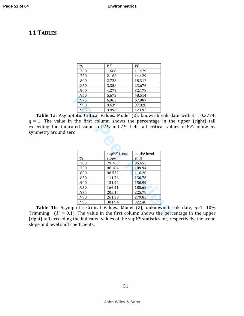
For Peer Review

51

11 TABLES

% VF .700 1.668 11.479 .750 2.166 14.429 .800 2.728 18.312 .850 3.388 23.676 .900 4.279 32.178 .950 5.673 48.514 .975 6.965 67.987 .990 8.639 97.928 .995 9.896 123.92

Table 1a: Asymptotic Critical Values. Model (2), known break date with , . The value in the first column shows the percentage in the upper (right) tail exceeding the indicated values of and . Left tail critical values of follow by symmetry around zero.

%

supVF trend slope

supVF level shift

.700 79.765 95.455

.750 88.184 109.94

.800 98.532 116.20

.850 111.78 130.76

.900 131.92 150.99

.950 166.41 188.68

.975 205.15 225.78

.990 261.39 279.85

.995 301.94 322.48

Table 1b: Asymptotic Critical Values. Model (2), unknown break date, q=1. 10% Trimming ( ). The value in the first column shows the percentage in the upper (right) tail exceeding the indicated values of the supVF statistics for, respectively, the trend slope and level shift coefficients.

of 64

John Wiley & Sons

Environmetrics

For Peer Review

52

Without Level Shift With Level Shift

120 0 0 .060 .055 .049 .063 .057 .051

0.3 0 .063 .089 .053 .067 .093 .056

0.6 0 .073 .126 .068 .080 .131 .070

0.9 0 .139 .256 .127 .141 .264 .116

0.3 0.3 .181 .176 .076 .175 .172 .079

0.6 0.3 .255 .293 .148 .247 .286 .129

0.9 -0.3 .021 .102 .053 .022 .117 .060

240 0 0 .054 .053 .049 .058 .056 .054

0.3 0 .059 .080 .053 .059 .081 .057

0.6 0 .066 .103 .060 .064 .106 .064

0.9 0 .103 .192 .092 .101 .200 .092

0.3 0.3 .175 .145 .064 .168 .139 .068

0.6 0.3 .217 .229 .106 .209 .229 .101

0.9 -0.3 .013 .083 .055 .017 .092 .059

636 0 0 .056 .054 .053 .049 .047 .048

0.3 0 .055 .071 .053 .049 .067 .049

0.9 0 .057 .082 .056 .053 .078 .051

0.9 0 .073 .128 .070 .068 .128 .065

0.3 0.3 .158 .105 .059 .151 .103 .052

0.6 0.3 .177 .153 .077 .169 .150 .071

0.9 -0.3 .008 .071 .053 .007 .070 .050

Table 2a: Empirical Null Rejections with AR(2) Errors. , 5% Nominal Level, , , . The data generating process is given by (17) and (18).

of 64

John Wiley & Sons

Environmetrics

For Peer Review

53

Without Level Shift With Level Shift

0 0 0 .01 .056 .054 .053 .049 .049 .048

.0105 .380 .378 .310 .144 .142 .127

.011 .912 .914 .816 .442 .439 .373

.012 .999 1.000 1.000 .949 .950 .881

.9 .01 .073 .130 .070 .069 .126 .066

.0105 .092 .153 .091 .073 .133 .073

.011 .148 .229 .142 .088 .158 .090

.012 .366 .484 .325 .160 .258 .143

0 .25 0 .01 .447 .443 .301 .049 .047 .048

.0105 .055 .055 .040 .144 .142 .127

.011 .319 .322 .213 .442 .439 .373

.012 .998 .998 .950 .949 .950 .881

.9 .01 .091 .158 .088 .069 .126 .066

.0105 .073 .128 .069 .073 .133 .073

.011 .089 .147 .084 .088 .158 .090

.012 .234 .324 .206 .160 .258 .143

.5 0 0 .01 .059 .056 .056 .050 .047 .047

.0105 .594 .595 .492 .226 .222 .187

.011 .995 .995 .963 .685 .679 .577

.012 1.000 1.000 1.000 .999 .999 .984

.9 .01 .073 .128 .072 .066 .127 .064

.0105 .106 .173 .101 .074 .142 .075

.011 .211 .304 .189 .108 .185 .101

.012 .572 .686 .495 .242 .350 .218

.5 .25 0 .01 .690 .691 .430 .050 .047 .047

.0105 .057 .056 .032 .226 .222 .187

.011 .508 .509 .303 .685 .679 .577

.012 1.000 1.000 .995 .999 .999 .984

.9 .01 .110 .179 .102 .066 .127 .064

.0105 .071 .126 .070 .074 .142 .075

.011 .098 .163 .094 .108 .185 .101

.012 .351 .467 .305 .242 .350 .218

Table 2b: Empirical Null Rejections and Empirical Power with AR(1) Errors. , T=636, 5% Nominal Level, , . The data generating process is given by (17) and (18).

of 64

John Wiley & Sons

Environmetrics

For Peer Review

54

Simple Trend Trend + Level shift Data Series

Model/ Obs Name Extra Forcings; No. runs

Trend (C/decade)

Std Error

Trend (C/decade)

Std Error

Level Shift (C/decade)

Std Error

1 BCCR BCM2.0 O; 2 0.173 0.0071

0.176 0.0128

-0.013 -0.0405

2 CC;CMA3.1-T47 NA; 5 0.347 0.0046

0.345 0.0084

0.008 0.0266

3 CCCMA3.1-T63 NA; 1 0.373 0.0094

0.393 0.0146

-0.078 -0.0462

4 CNRM3.0 O; 1 0.249 0.0061

0.237 0.0106

0.044 0.0333

5 CSIRO3.0 1 0.139 0.0087

0.170 0.0183

-0.114 -0.0577

6 CSIRO3.5 1 0.242 0.0093

0.296 0.0136

-0.203 -0.0429

7 GFDL2.0 O, LU, SO, V; 1 0.186 0.0120

0.141 0.0235

0.170 0.0742

8 GFDL2.1 O, LU, SO, V; 1 0.109 0.0184

0.135 0.0319

-0.097 -0.1007

9 GISS_AOM 2 0.171 0.0085

0.156 0.0142

0.058 0.0449

10 GISS_EH O, LU, SO, V; 6 0.193 0.0117

0.226 0.0174

-0.121 -0.0551

11 GISS_ER O, LU, SO, V; 5 0.178 0.0137

0.207 0.0219

-0.110 -0.0690

12 IAP_FGOALS1.0 3 0.198 0.0132

0.243 0.0187

-0.170 -0.0591

13 ECHAM4 1 0.210 0.0140

0.236 0.0227

-0.096 -0.0717

14 INMCM3.0 SO, V; 1 0.178 0.0094

0.174 0.0169

0.015 0.0533

15 IPSL_CM4 1 0.189 0.0074

0.159 0.0126

0.114 0.0397

16 MIROC3.2_T106 O, LU, SO, V; 1 0.141 0.0104

0.121 0.0169

0.076 0.0534

17 MIROC3.2_T42 0.210 0.0133 0.233 0.0212 -0.086 -0.0669

of 64

John Wiley & Sons

Environmetrics

For Peer Review

55

Table 3: Summary of Lower Troposphere data series. Notes: Each row refers to model ensemble mean (rows 1—23) or observational series (rows 24—26). All models forced with 20th century greenhouse gases and direct sulfate effects. Rows 10, 11, 19, 22 and 23 also include indirect sulfate effects. ‘Extra forcing’ indicates which models included other forcings: ozone depletion (O), solar changes (SO), land use (LU), volcanic eruptions (V). NA: information not supplied to PCMDI. No. runs: indicates number of individual realizations in the ensemble mean. Trend slopes estimated using OLS, Std Errors computed using VF method (see Section 4).

O, LU, SO, V; 3 18 MPI2.3.2a

SO, V; 5 0.205 0.0141

0.231 0.0228

-0.096 -0.0721 19 ECHAM5

O; 4 0.204 0.0059

0.198 0.0109

0.023 0.0343 20 CCSM3.0

O, SO, V; 7 0.217 0.0161

0.262 0.0236

-0.167 -0.0744 21 PCM_B06.57

O, SO, V; 4 0.176 0.0060

0.169 0.0114

0.024 0.0361 22 HADCM3

O; 1 0.190 0.0062

0.190 0.0114

0.001 0.0359 23 HADGEM1

O, LU, SO, V; 1 0.226 0.0104

0.205 0.0202

0.078 0.0636 24 HadAT 0.135 0.0093 0.064 0.0209 0.270 0.0660 25 RICH 0.134 0.0092 0.093 0.0206 0.155 0.0651 26 RAOBCORE 0.147 0.0080 0.065 0.0166 0.308 0.0525

of 64

John Wiley & Sons

Environmetrics

For Peer Review[56]

Simple Trend Trend + Level shift Data Series

Model/ Obs Name Extra Forcings; No. runs

Trend

(C/decade)

Std Error

Trend

(C/decade)

Std Error

Level Shift (C/decade)

Std Error

1 BCCR BCM2.0 O; 2 0.176 0.0060

0.184 0.0107

-0.030 0.0336

2 CC;CMA3.1-T47 NA; 5 0.372 0.0046

0.365 0.0084

0.026 0.0265

3 CCCMA3.1-T63 NA; 1 0.399 0.0093

0.417 0.0149

-0.068 0.0471

4 CNRM3.0 O; 1 0.311 0.0072

0.296 0.0125

0.057 0.0395

5 CSIRO3.0 1 0.108 0.0086

0.139 0.0182

-0.117 0.0575

6 CSIRO3.5 1 0.229 0.0097

0.286 0.0142

-0.213 0.0448

7 GFDL2.0 O, LU, SO, V; 1 0.174 0.0117

0.133 0.0229

0.155 0.0722

8 GFDL2.1 O, LU, SO, V; 1 0.103 0.0198

0.143 0.0333

-0.152 0.1051

9 GISS_AOM 2 0.163 0.0081

0.154 0.0141

0.031 0.0446

10 GISS_EH O, LU, SO, V; 6 0.180 0.0114

0.210 0.0172

-0.114 0.0542

11 GISS_ER O, LU, SO, V; 5 0.162 0.0127

0.182 0.0211

-0.076 0.0666

12 IAP_FGOALS1.0 3 0.185 0.0125

0.225 0.0182

-0.149 0.0575

13 ECHAM4 1 0.200 0.0131

0.218 0.0220

-0.068 0.0696

of 64

John Wiley & Sons

Environmetrics

For Peer Review[57]

14 INMCM3.0 SO, V; 1 0.183 0.0100

0.173 0.0175

0.035 0.0551

15 IPSL_CM4; 1 0.195 0.0081

0.157 0.0130

0.140 0.0411

16 MIROC3.2_T106 O, LU, SO, V; 1

0.147

0.0113

0.119 0.0175

0.105 0.0553

17 MIROC3.2_T42 O, LU, SO, V; 3 0.211 0.0143

0.234 0.0231

-0.086 0.0728

18 MPI2.3.2a SO, V; 5 0.182 0.0124

0.193 0.0214

-0.045 0.0675

19 ECHAM5 O; 4 0.202 0.0059

0.197 0.0109

0.018 0.0345

20 CCSM3.0 O, SO, V; 7 0.201 0.0132

0.232 0.0203

-0.116 0.0640

21 PCM_B06.57 O, SO, V; 4 0.161 0.0048

0.136 0.0084

0.096 0.0266

22 HADCM3 O; 1 0.170 0.0059

0.166 0.0109

0.134 0.0344

23 HADGEM1 O, LU, SO, V; 1 0.221 0.0108

0.210 0.0207

0.041 0.0653

24 HadAT 0.089 0.0088 -0.001 0.0172 0.336 0.0542 25 RICH 0.096 0.0075 0.048 0.0225 0.180 0.0709 26 RAOBCORE 0.132 0.0082 0.042 0.0152 0.339 0.0478

Table 4: Summary of Mid-Troposphere data series. Notes same as for Table 3.

of 64

John Wiley & Sons

Environmetrics

For Peer Review

58

Trend Coef Null Hypothesis Test Score Bootstrap p value

No Level shift Hadley LT (0.135) trend = 0 213.3*** < 0.001 RICH LT (0.134) trend = 0 212.7*** < 0.001 RAOBCORE LT (0.147) trend = 0 337.5*** < 0.001 Hadley MT (0.089) trend = 0 102.8*** < 0.001 RICH MT (0.096) trend = 0 94.1*** < 0.001 RAOBCORE MT(0.132) trend = 0 259.8*** < 0.001 LT Models = Observed 96.2*** < 0.001 MT Models = Observed 155.4*** < 0.001

With Level shift at Date (Assumed Known): December 1977 Hadley LT (0.064) trend = 0 9.2 0.349 RICH LT (0.093) trend = 0 20.4 0.180 RAOBCORE LT (0.065) trend = 0 15.4 0.235 Hadley MT (-0.001) trend = 0 0.001 0.991 RICH MT (0.048) trend = 0 4.6 0.498 RAOBCORE MT (0.042) trend = 0 7.7 0.388 LT Models = Observed 261.1*** < 0.0002 MT Models = Observed 423.1*** < 0.0001

With Level Shift at Date Assumed Unknown LT Models = Observed 352.14*** < 0.001 MT Models = Observed 544.08*** < 0.001

Table 5: Results of hypothesis tests using VF statistic with and without level shift term at December, 1977. Notes: sample period (monthly): January 1958 to December 2010. The bootstrap p-value* is computed using the method described in Section 3.3 using 10000 bootstrap replications. VF Critical Values: Without level shift, 20.14 (10%, denoted *) 41.53 (5%, denoted **), 83.96 (1%, denoted ***). With level shift at known date, 32.32 (10%, denoted *), 49.03 (5%, denoted **), 97.23 (1%, denoted ***). With level shift at unknown date, 131.92 (10%, denoted *), 166.41 (5%, denoted **), 261.39 (1%, denoted ***).

of 64

John Wiley & Sons

Environmetrics

For Peer Review

59

LT Layer MT Layer

Model

No Break

Known Break Date

Unknown Break Date

No Break

Known Break Date

Unknown Break Date

1 24.00* 53.35** 53.55 80.32** 206.48*** 115.54 2 750.18*** 231.96*** 731.85*** 1497.65*** 724.02*** 1078.92*** 3 653.13*** 913.03*** 924.73*** 636.38*** 1898.60*** 1446.43*** 4 107.71*** 48.37* 136.51* 469.47*** 192.48*** 378.75*** 5 0.00 7.78 14.09 0.43 16.17 11.96 6 79.02** 106.07*** 108.73 93.27*** 222.04*** 159.70* 7 31.53* 17.88 38.68 58.72** 47.08* 67.93 8 4.12 8.16 51.00 0.04 24.93 45.61 9 5.50 7.55 36.98 31.29* 29.52 49.78 10 28.38* 288.26*** 350.18*** 36.83* 495.44*** 476.83*** 11 11.65 150.50*** 170.06** 20.40* 192.87*** 241.43** 12 25.62* 297.75*** 363.07*** 35.91* 466.40*** 494.46*** 13 43.33** 378.37*** 453.11*** 53.93** 339.05*** 606.04*** 14 6.16 8.65 35.57 37.72* 27.26 61.59 15 27.03* 17.11 56.02 116.07*** 57.92** 97.57 16 0.03 2.61 42.62 19.89 15.83 47.48 17 37.32* 324.54*** 335.89*** 46.86** 231.36*** 350.56*** 18 29.94* 194.02*** 248.19*** 36.14* 186.32*** 285.08*** 19 53.03** 38.01* 92.42 159.76*** 156.99*** 127.39 20 29.92* 280.15*** 349.58*** 45.43** 372.73*** 563.97*** 21 31.54* 45.95* 53.44 142.56*** 130.34*** 92.19 22 34.89** 35.84* 52.27 64.75** 80.93** 77.74 23 144.28*** 94.78*** 143.16* 143.26*** 235.49*** 292.16*** <=5% 8/23 12/23 9/23 14/23 17/23 11/23

Table 6. VF tests of equivalent trends between individual model (ensemble mean in cases of multiple runs) and average of balloon series. Column 1: model. Column 2: LT layer, No Break case. Columns 3 and 4 (Break1 and Break2, respectively): with break assumed known at 1977:12 and with break at date assumed unknown. Columns 5-7: same for MT layer. VF Critical Values: Without level shift, 20.14 (10%, denoted *) 41.53 (5%, denoted **), 83.96 (1%, denoted ***). With level shift known to be at 1977:12, 33.32 (10%, denoted *), 51.20 (5%, denoted **), 98.46 (1%, denoted ***). With level shift at unknown date, 131.92 (10%, denoted *), 166.41 (5%, denoted **), 261.39 (1%, denoted ***). Last row: fraction of models exhibiting difference from observations significant at <=5%.

of 64

John Wiley & Sons

Environmetrics

For Peer Review

Figure 1. Schematics of two series to be compared. 135x132mm (96 x 96 DPI)

of 64

John Wiley & Sons

Environmetrics

For Peer Review

Figure 2. Radiosonde series. Left column: Lower Troposphere. Right column: Mid-Troposphere. Top row: HadAT series. Middle row: RICH series. Bottom row: RAOBCORE series. Least squares trends shown.

101x73mm (300 x 300 DPI)

of 64

John Wiley & Sons

Environmetrics

For Peer Review

Figure 3. Model-Observation comparisons allowing for level shift after 1977:12. Left: LT layer, dots indicate monthly data from 3 GCMs, black line, trend through all GCMs, gray dashed line, trend through average of three radiosonde series allowing for step-change at 1977:12. Observed series are shifted down so starting

value coincides with that of model average. Right: same for MT layer. 101x73mm (300 x 300 DPI)

of 64

John Wiley & Sons

Environmetrics

For Peer Review

Figure 4. 1958-2010 Trends and 95% CIs for 23 models (shaded region) and three radiosonde series Hadley, RICH and RAOBCORE (respectively, individual markers at right edge). Top row: Trends computed without allowing for level shift. Bottom row: Level shift term included in model. Left column: LT. Right

column: MT. 101x73mm (300 x 300 DPI)

of 64

John Wiley & Sons

Environmetrics

For Peer Review

Figure 5. Grid search of VF scores of model-observational equivalence varying the break point across the middle 80% of the sample. Top: LT. Bottom: MT. Horizontal lines show 10%, 5%, and 1% critical values (resp. 131.92, 166.41 and 261.39). Maximum values are at obs 257 352.1 (LT) and obs 250 544.1 (MT).

101x73mm (300 x 300 DPI)

of 64

John Wiley & Sons

Environmetrics

for peer review - tulane universityeconomic/seminars/vogelsang_climate.pdf · the presence of...

Documents