DESIGN AND ANALYSIS OF A 10” CARBON FIBER WHEEL

FOR A FORMULA SAE RACECAR

by

PRATIK BHAGWAT

Presented to the Faculty of the Graduate School of

The University of Texas at Arlington in Partial Fulfillment

of the Requirements

for the Degree of

MASTER OF SCIENCE IN MECHANICAL ENGINEERING

THE UNIVERSITY OF TEXAS AT ARLINGTON

May 2017

ii

Copyright © by Pratik Bhagwat 2017

All Rights Reserved

iii

Dedicated to my mother, Swati Bhagwat, for her unconditional love

and my sisters, Deepti and Kavita, for their continued support and motivation.

1

Acknowledgements

I would like to thank my supervising professor Dr. Robert L. Woods for his

continued guidance while helping me develop a professional attitude and for his

invaluable support and faith in me. I highly appreciate the time invested by him for the

successful completion of this project while providing logical reasoning through technical

debates regarding the design.

This project would have been impossible to achieve without the support of UTA

Racing team members, Priyank Nandu, Amogh Taraikar and Scott Berggren. With their

advice, it was possible for me to accelerate my learning of HyperWorks design software

and enhance my knowledge on carbon fiber composites.

I would like to express my gratitude towards my mother without whom I may have

been unable to pursue higher education at UTA. Lastly, I’d like to thank all my friends for

their companionship during my 2 years at UTA.

April 28, 2017

2

Abstract

DESIGN AND ANALYSIS OF A 10” CARBON FIBER WHEEL

FOR A FORMULA SAE RACECAR

Pratik Bhagwat, MS

The University of Texas at Arlington, 2017

Supervising Professor: Robert L. Woods

Formula SAE is an engineering design competition for students where the goal is

to design, build, and compete a Formula-style single seater race vehicle. With a legacy

dating back to 1982, UTA Racing has been one of the most competitive teams.

In this project, a carbon fiber 10” wheel is designed for the first time, achieving

reduced unsprung weight and lower rotational inertia, both of which are key performance

characteristics in vehicle dynamics. The design follows Tire and Rim Association

guidelines to ensure dimensional compatibility and ease of assembly and is analyzed for

2G cornering with 3G bump. The simulations were executed for 16 configurations based

on a parametric design. The project also includes the design and analysis of a modular

wheel mold that allows for possibility to manufacture several wheels with varying, width,

locking mechanism and weight reduction patterns for future design changes.

The wheel design selected for manufacturing is compared for factor of safety,

weight and wheel deflection with the other configurations. This wheel is estimated to

weigh 1.8 lbs, demonstrating 29% weight reduction on the existing 10” carbon fiber-

aluminum wheel assembly.

3

Table of Contents

Acknowledgements ............................................................................................................. 1

Abstract ............................................................................................................................... 2

List of Illustrations ............................................................................................................... 6

Abbreviations ...................................................................................................................... 9

Chapter 1 : Introduction..................................................................................................... 10

1.1 Weight reduction in FSAE ...................................................................................... 10

1.2 Unsprung mass of a vehicle ................................................................................... 11

1.3 Moment of Inertia .................................................................................................... 11

1.4 UTA Racing Carbon Wheels .................................................................................. 12

1.5 Objective ................................................................................................................. 15

Chapter 2 Design study..................................................................................................... 17

2.1 Design Ideology ...................................................................................................... 17

2.2 Existing Carbon Fiber Wheels ................................................................................ 17

Chapter 3 Design Iterations .............................................................................................. 22

3.1 Iteration Nomenclature ........................................................................................... 23

3.1 Parametric sketch ................................................................................................... 24

3.2 Geometry considerations ........................................................................................ 26

Keep out zone .......................................................................................................... 26

Surface continuity and draft angle ............................................................................ 26

Wheel offset and backspacing ................................................................................. 26

Wheel bead and lip ................................................................................................... 28

3.3 Major Spoke Iterations ............................................................................................ 29

C Cross section ........................................................................................................ 29

4

Semi Hexagonal cross section ................................................................................. 30

T-cross section ......................................................................................................... 30

Hollow spoke, Tubular section ................................................................................. 31

Curved planar section............................................................................................... 31

Chapter 4 Finite Element Analysis .................................................................................... 32

4.1SolidWorks iteration ................................................................................................. 32

Material ..................................................................................................................... 32

Setup ........................................................................................................................ 33

Fixed Geometry .................................................................................................... 33

External Loads ..................................................................................................... 33

Result........................................................................................................................ 35

4.2 Comparative study of SolidWorks iterations ........................................................... 36

4.3 HyperWorks ............................................................................................................ 37

Surface Model Generation ....................................................................................... 37

Material properties .................................................................................................... 38

Meshing .................................................................................................................... 39

Ply orientation ........................................................................................................... 40

Setup ........................................................................................................................ 41

Results ...................................................................................................................... 41

Mold Design ..................................................................................................... 43

Modularity ................................................................................................................. 43

Mold design in SolidWorks ....................................................................................... 44

Draft analysis ............................................................................................................ 46

Thermal expansion ................................................................................................... 47

Conclusion and Future Scope .......................................................................... 48

5

Appendix A Solidworks Iteration Illustrations .................................................................... 49

Appendix B HyperWorks guide ......................................................................................... 68

References ...................................................................................................................... 100

Biographical Information ................................................................................................. 102

6

List of Illustrations

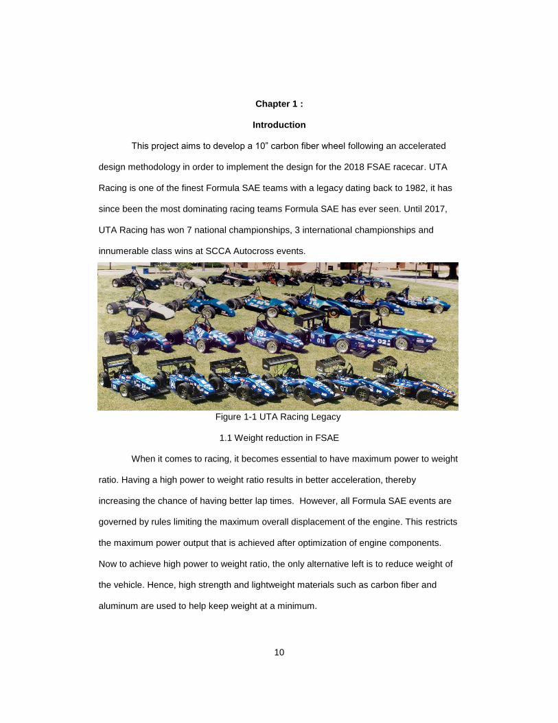
Figure 1-1 UTA Racing Legacy ......................................................................................... 10

Figure 1-2 UTA Racing's 1993 car with carbon wheels .................................................... 12

Figure 1-3 2003-Wheel assembly CAD ............................................................................ 12

Figure 1-4 Wheel design from 2003 .................................................................................. 12

Figure 1-5 10"x6" Wheel Mold and Prototype ................................................................... 13

Figure 1-6 10”x7” Wheel assembly for UTA Racing’s 2017 Racecar ............................... 14

Figure 2-1 Joanneum Racing’s non-hollow wheel ............................................................ 18

Figure 2-2 Joaneum Racing wheel ................................................................................... 18

Figure 2-3 TU Graz's Racing wheel section ..................................................................... 18

Figure 2-4 TU Graz’s Racing Wheel ................................................................................. 18

Figure 2-5 Team Bath Racing wheel ................................................................................ 19

Figure 2-6 Exploded view of the wheel ............................................................................. 19

Figure 2-7 JMS Wheel layup ............................................................................................. 19

Figure 2-8 JMS Wheel Prototype ...................................................................................... 19

Figure 2-9 Carbon Revolution thermal barrier coating ...................................................... 20

Figure 2-10 Cross section of Shelby GT350R's carbon wheels. ...................................... 20

Figure 2-11 Regera's hollow wheel design ....................................................................... 21

Figure 2-12 Koenigsegg’s 5-spoke wheel ......................................................................... 21

Figure 2-13 5-spoke Wheel mold ...................................................................................... 21

Figure 3-1 Iterative Design process .................................................................................. 22

Figure 3-2 TRA Specifications for 10" Rim ....................................................................... 24

Figure 0-3 Parametric sketch of Wheel Rim Profile .......................................................... 25

Figure 3-4 Dimension for editing number of plies ............................................................. 25

7

Figure 3-5 Keep-out zone ................................................................................................. 26

Figure 3-6 Continuous lay-up surface ............................................................................... 26

Figure 3-7 UTA Racing's offset and backspacing ............................................................. 27

Figure 3-8 Wheel offset ..................................................................................................... 27

Figure 3-9 Wheel assembly cross section with bead and lip ............................................ 28

Figure 3-10 Load paths along the wheel spokes .............................................................. 29

Figure 3-11 Iteration BH and BO with C cross section spoke........................................... 29

Figure 3-12 Iterations BJ and BM showing semi-hexagonal sections .............................. 30

Figure 3-13 Iteration BP with the T-cross section wheel spoke ........................................ 30

Figure 3-14 Iteration BR with hollow spoke design ........................................................... 31

Figure 3-15 Iterations BW and BU with curved-planar section ......................................... 31

Figure 4-1 SolidWorks material Al 6061 T6 ...................................................................... 32

Figure 4-2 Zero displacement of hub contact surface ...................................................... 33

Figure 4-3 Fixed geometry for drive pins .......................................................................... 33

Figure 4-4 Remote load application .................................................................................. 34

Figure 4-5 Clamping force on inboard and outboard ........................................................ 34

Figure 4-6 Factor of safety plot for iteration BS ................................................................ 35

Figure 4-7 Displacement plot for iteration BS ................................................................... 35

Figure 4-8 Comparative study of iterations ....................................................................... 36

Figure 4-9 Center line geometry for surface generation ................................................... 37

Figure 4-10 Surface model preview with cross section .................................................... 38

Figure 4-11 E7653 Laminate Properties ........................................................................... 39

Figure 4-12 Meshing preview. ........................................................................................... 39

Figure 4-13 Ply orientation for wheel center ..................................................................... 40

Figure 4-14 Cross section with ply distribution ................................................................. 41

8

Figure 4-15 Composite Failure ......................................................................................... 42

Figure 4-16 Max dispacement .......................................................................................... 42

Figure 5-1 Modular mold CAD assembly .......................................................................... 43

Figure 5-2 Wheel center mold model tree......................................................................... 44

Figure 5-3 Extrude bar for wheel mold .............................................................................. 45

Figure 5-4 Summarized wheel center mold design process ............................................. 45

Figure 5-5 Draft analysis on mold components ................................................................ 46

Figure 5-6 Thermal Expansion variables .......................................................................... 47

9

Abbreviations

CF: Carbon Fiber

FSAE: Formula SAE

SCCA: Sports Car Club of America

CAD: Computer Aided Design

CAE: Computer Aided Engineering

TRA: Tire and Rim Association

10

Chapter 1 :

Introduction

This project aims to develop a 10” carbon fiber wheel following an accelerated

design methodology in order to implement the design for the 2018 FSAE racecar. UTA

Racing is one of the finest Formula SAE teams with a legacy dating back to 1982, it has

since been the most dominating racing teams Formula SAE has ever seen. Until 2017,

UTA Racing has won 7 national championships, 3 international championships and

innumerable class wins at SCCA Autocross events.

1.1 Weight reduction in FSAE

When it comes to racing, it becomes essential to have maximum power to weight

ratio. Having a high power to weight ratio results in better acceleration, thereby

increasing the chance of having better lap times. However, all Formula SAE events are

governed by rules limiting the maximum overall displacement of the engine. This restricts

the maximum power output that is achieved after optimization of engine components.

Now to achieve high power to weight ratio, the only alternative left is to reduce weight of

the vehicle. Hence, high strength and lightweight materials such as carbon fiber and

aluminum are used to help keep weight at a minimum.

Figure 1-1 UTA Racing Legacy

11

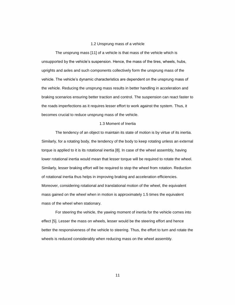
1.2 Unsprung mass of a vehicle

The unsprung mass [11] of a vehicle is that mass of the vehicle which is

unsupported by the vehicle’s suspension. Hence, the mass of the tires, wheels, hubs,

uprights and axles and such components collectively form the unsprung mass of the

vehicle. The vehicle’s dynamic characteristics are dependent on the unsprung mass of

the vehicle. Reducing the unsprung mass results in better handling in acceleration and

braking scenarios ensuring better traction and control. The suspension can react faster to

the roads imperfections as it requires lesser effort to work against the system. Thus, it

becomes crucial to reduce unsprung mass of the vehicle.

1.3 Moment of Inertia

The tendency of an object to maintain its state of motion is by virtue of its inertia.

Similarly, for a rotating body, the tendency of the body to keep rotating unless an external

torque is applied to it is its rotational inertia [8]. In case of the wheel assembly, having

lower rotational inertia would mean that lesser torque will be required to rotate the wheel.

Similarly, lesser braking effort will be required to stop the wheel from rotation. Reduction

of rotational inertia thus helps in improving braking and acceleration efficiencies.

Moreover, considering rotational and translational motion of the wheel, the equivalent

mass gained on the wheel when in motion is approximately 1.5 times the equivalent

mass of the wheel when stationary.

For steering the vehicle, the yawing moment of inertia for the vehicle comes into

effect [5]. Lesser the mass on wheels, lesser would be the steering effort and hence

better the responsiveness of the vehicle to steering. Thus, the effort to turn and rotate the

wheels is reduced considerably when reducing mass on the wheel assembly.

12

1.4 UTA Racing Carbon Wheels

UTA Racing was the first team ever to use a carbon composite wheel. In 1993,

the first carbon fiber wheel was demonstrated in FSAE.

In 2003, an updated wheel design was implemented. The wheel design

demonstrated a carbon fiber wheel rim with an aluminum rim center. The CF rim would

locate the tire, while the wheel center would connect the hub to the CF rim. This setup

allowed for change of wheel center design while achieving high wheel stiffness. It is

required to have minimum wheel deflections to maintain the slip angle. The carbon rim

Figure 1-2 UTA Racing's 1993 car with carbon wheels

Figure 1-4 Wheel design from 2003 Figure 1-3 2003-Wheel assembly CAD

13

mold has been useful until 2016, while slight modifications with the wheel center allowed

for better packaging and weight reduction The wheel centers were attached to the

carbon rim by using the “huck” fasteners which are a combination of high performance

Huck bolts and structural blind fasteners. It is similar to riveting while being threaded.

In the past, there have been attempts at making a 10’’ wheel with a width of 6’’ to

experiment the benefits of a 10” wheel package. However, on manufacturing a prototype

wheel using fiberglass as the material, the wheel could not be successfully cured and a

failure was observed at the merging surfaces. Also, the 6” width was then replaced by a

7” tire rendering the mold futile. Other issues were epoxy of metal lugs would induce

errors during curing of the fibers.

Failure edge

Figure 1-5 10"x6" Wheel Mold and Prototype

14

In 2017, UTA Racing underwent a complete design change with a 10”

wheel package design with a 7” width due to the availability of superior performance

Hoosier racing tires. This wheel package showcased a center locking mechanism to

attach with the hub due to weight reduction advantage over the traditional 4 and 3 lug

patterns.

This required the need for a new mold. A 10” CF rim with an aluminum rim

center was designed and manufactured. This wheel assembly weighed 2.51 lbs. The

fastening method was similar to the 2003 design. It used Huck fasteners to attach the

wheel center to the CF rim. The wheel center had provisions for 3 drive pins to transmit

the torque from the hubs to the wheels. This project aims to replace this assembly with a

full carbon fiber wheel.

Figure 1-6 10”x7” Wheel assembly for UTA Racing’s 2017 Racecar

15

1.5 Objective

The objective of this project is to replace the 2017 10” wheel assembly with a full

carbon fiber model. The primary targets of these designs are as follows:

1. Achieve minimum 15% weight reduction

2. Have wheel stiffness equivalent or better with respect to the existing wheel assembly

3. Implement direct modelling in parametric environment for ease of modification

4. Design a modular wheel mold with variable wheel width, variable wheel center

pattern, possibility to switch to traditional lugs for fastening of the wheel to the hub

5. Reduce overall cost and manufacturing time

With the existing wheel design, the elimination of using 6 Huck fasteners would

result in a 4% weight reduction and exclude the requirement of using special tools for

their installation. The 2nd objective is crucial to maintain the slip angles induced due to tire

and wheel deflection. These two objectives would result in improved performance with

respect to vehicle dynamics by reduction in unsprung mass and rotational inertia while

maintaining the slip angles. Parametric modelling is a term used in Computer-Aided

Design language that refers to design geometries which are easy to modify without failing

features and constraints. Direct modelling on the other hand gives freedom to change

every dimension that may result in unrealistic design geometries and failing features,

which require redesign resulting in tremendous time loss. Direct modelling in a parametric

environment on the other hand benefits the end user who can modify the dimensions

such as fillets, wheel patterns and hole sizes without failing the features. These

dimensions are locked to certain limit that would prevent breaking any design constraint

such as the dimensions provided by the Tire and Rim Association. This approach helps

to accelerate design, improve quality and allow for innovation in design.

16

UTA Racing designs FSAE racecars every year. Hence the vehicle dynamics

change every year too, resulting in variations in load acting on the wheel. Also, there

might be a possibility of a new tire being available but with a different width. In such

cases, having a modular mold will allow modification of design of the wheel preventing

futility of the mold in the future. This objective was taken into consideration due to failure

to use the previous 10” wheel mold. My objective is to design a mold to that would allow

manufacturing wheel molds with width ranging from 6” to 8”. The mold should also allow

change of wheel offset, which is the dimension that defines the mounting of the hub onto

the wheel. Having the ability to switch from a center locking nut arrangement to a

traditional 4 or 3 lug design is an added advantage of the modular mold. The modular

mold will require manufacturing of certain sections to allow the above flexibility in design.

The last objective being saving cost and manufacturing time is established since

the wheel shall be manufactured in-house by UTA Racing students and not by

professionals. The cost of manufacturing aluminum rim centers will be eliminated while

also saving manufacturing time. There is substantial saving in cost in purchasing

aluminum stock bar used for the existing wheel centers. However, the object is to ensure

the cost saved in elimination of wheel center manufacturing is under the cost of carbon

fiber that shall be used for the manufacturing of the wheel. This will result in considerable

cost and time savings in manufacturing each wheel.

17

Chapter 2

Design study

As mentioned earlier, in this project, I have opted for an accelerated design

approach. To enable myself in studying maximum design possibilities, I chose

SolidWorks® 2016 as my CAD tool. UTA Racing is sponsored with student edition of the

software allowing me better accessibility as I continued to pursue racecar engineering.

Final analysis for ply based geometry were studied using Altair HyperWorks® v14.0 which

was also sponsored to UTA Racing. Over the course of the study, 32 iterations were

designed based on ease of manufacturing and surface continuity. However, 16 of the

iterations were scrapped due to major changes in the hub design. In this report, I have

discussed the other 16 iterations which can be implemented on UTA Racing’s 2017

racecar.

2.1 Design Ideology

The design ideology was to get a uniform stress distribution over the geometry.

Since the torque was to be transferred by 3 drive pins, in order to provide a distributed

load path, the number of spokes were considered to be in multiples of 3. Also,

considering the loading directions, the spoke cross section geometry was analyzed to

have maximum stiffness for minimum displacement. To get a head start with the design,

existing FSAE and commercially available CF wheels were investigated.

2.2 Existing Carbon Fiber Wheels

UTA Racing has interacted with various teams during competitions. One such

team was TU Graz Racing team from Graz University of technology, Austria. At Formula

SAE Michigan 2015, TU Graz Racing team generously shared information on their 3

spoke hollow wheel design which they have been successfully using for years. They use

trapped rubber molding to get hollow spokes for weight reduction and stiffness.

18

The TU Graz Racing wheel is also designed for center locking mechanism with 3

drive pins. On similar lines, Joanneum Racing team from University of Applied Sciences,

Graz also have been highly successful with their hollow carbon wheel. They had

previously designed a non-hollow carbon wheel but later switched to a 3 spoke wheel

design. Both, TU Graz Racing and Joanneum Racing have used these wheels for over 2

years

Figure 2-1 Joanneum Racing’s non-hollow wheel

Figure 2-3 TU Graz's Racing wheel section Figure 2-4 TU Graz’s Racing Wheel

Figure 2-2 Joaneum Racing wheel

19

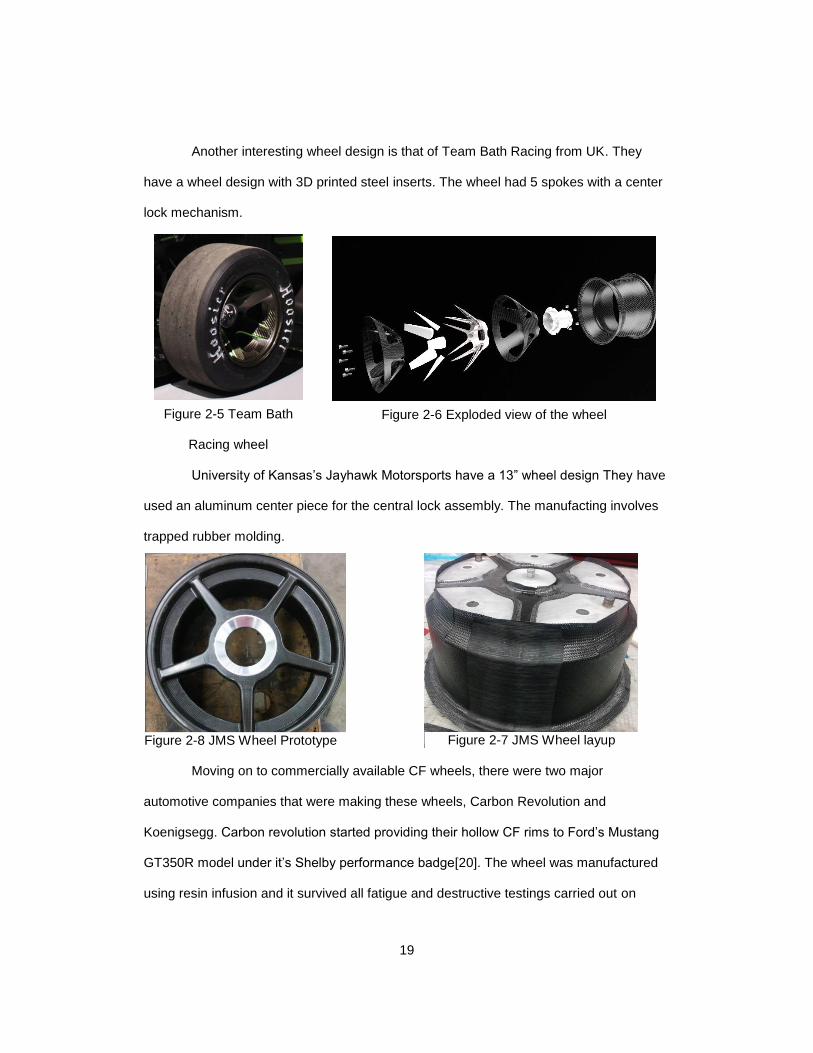
Another interesting wheel design is that of Team Bath Racing from UK. They

have a wheel design with 3D printed steel inserts. The wheel had 5 spokes with a center

lock mechanism.

University of Kansas’s Jayhawk Motorsports have a 13” wheel design They have

used an aluminum center piece for the central lock assembly. The manufacting involves

trapped rubber molding.

Moving on to commercially available CF wheels, there were two major

automotive companies that were making these wheels, Carbon Revolution and

Koenigsegg. Carbon revolution started providing their hollow CF rims to Ford’s Mustang

GT350R model under it’s Shelby performance badge[20]. The wheel was manufactured

using resin infusion and it survived all fatigue and destructive testings carried out on

Figure 2-5 Team Bath

Racing wheel

Figure 2-6 Exploded view of the wheel

Figure 2-7 JMS Wheel layup Figure 2-8 JMS Wheel Prototype

20

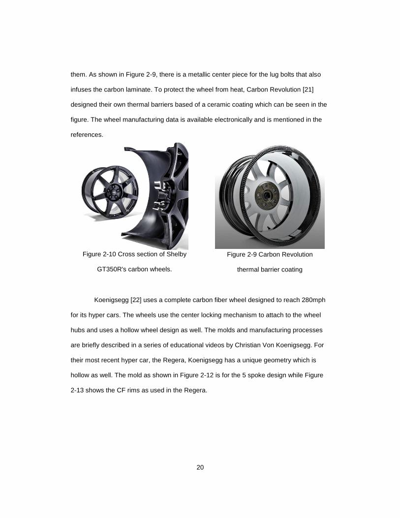
them. As shown in Figure 2-9, there is a metallic center piece for the lug bolts that also

infuses the carbon laminate. To protect the wheel from heat, Carbon Revolution [21]

designed their own thermal barriers based of a ceramic coating which can be seen in the

figure. The wheel manufacturing data is available electronically and is mentioned in the

references.

Koenigsegg [22] uses a complete carbon fiber wheel designed to reach 280mph

for its hyper cars. The wheels use the center locking mechanism to attach to the wheel

hubs and uses a hollow wheel design as well. The molds and manufacturing processes

are briefly described in a series of educational videos by Christian Von Koenigsegg. For

their most recent hyper car, the Regera, Koenigsegg has a unique geometry which is

hollow as well. The mold as shown in Figure 2-12 is for the 5 spoke design while Figure

2-13 shows the CF rims as used in the Regera.

Figure 2-9 Carbon Revolution

thermal barrier coating

Figure 2-10 Cross section of Shelby

GT350R's carbon wheels.

21

UTA Racing’s composite team identified the possibilities of manufacturing the

above discussed designs. Based on the experience and manufacturing options, certain

design goals were set and a detailed iterative study was initiated.

Figure 2-13 5-spoke Wheel mold

Figure 2-12 Koenigsegg’s 5-spoke wheel

Figure 2-11 Regera's hollow wheel design

22

Chapter 3

Design Iterations

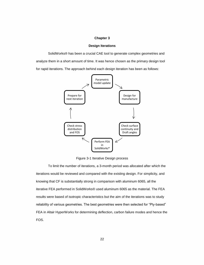
SolidWorks® has been a crucial CAE tool to generate complex geometries and

analyze them in a short amount of time. It was hence chosen as the primary design tool

for rapid iterations. The approach behind each design iteration has been as follows:

Figure 3-1 Iterative Design process

To limit the number of iterations, a 3-month period was allocated after which the

iterations would be reviewed and compared with the existing design. For simplicity, and

knowing that CF is substantially strong in comparison with aluminum 6065, all the

iterative FEA performed in SolidWorks® used aluminum 6065 as the material. The FEA

results were based of isotropic characteristics but the aim of the iterations was to study

reliability of various geometries. The best geometries were then selected for “Ply-based”

FEA in Altair HyperWorks for determining deflection, carbon failure modes and hence the

FOS.

Parametric model update

Design for manufacture

Check surface continuity and

Draft angles

Perform FEA in

SolidWorks®

Check stress distribution

and FOS

Prepare for next iteration

23

3.1 Iteration Nomenclature

UTA Racing follows a part numbering and nomenclature system to determine the

car year, assembly system, component code, iteration number, part name and designer

initial for ease of documentation. Each wheel design was hence named as “F17-WT-

00011-Bx-Carbon wheel_PB” where Bx represents the iteration number. BW in the

shown figure corresponds to 023, W being the 23rd iteration. Similarly, BA would mean

iteration 001, BB would correspond to 002 and so on.

Referring the Figure 3-2, the model tree as shown on the left represents the

design process for direct modelling in a parametric environment. The “Wheel

profile_revolve” has the parametric sketch for the wheel profile. “Drive pin hole”

determines the depth and location of the drive pin holes. “Wheel center pattern” is cut-

extrude feature for wheel spoke pattern on the wheel. The “Hub surface” is for isolating

the hub surface for loaded cases while performing FEA.

Figure 3-0 SolidWorks workspace(above) and

model tree (left)

24

3.1 Parametric sketch

Using the Tire and Rim Association specifications as shown in Figure 3-2, a

parametric sketch was modelled as the primary sketch which is revolved extruded to form

the wheel rim. The aim of this sketch was that any changes on this sketch should allow

the entire geometry to be recreated without the failure of any features. This parametric

sketch is also equation based. The equations were simple multiplier dimensions based

on the thickness of the CF ply.

The parametric sketch is complicated to decipher if viewed independently.

However, reviewing the sketch with the TRA spec simultaneously would give a better

understanding of the dimensions. These dimensions are locked for editing and are read

Figure 3-2 TRA Specifications for 10" Rim

25

only dimensions. The remaining dimensions are relative to the geometry for dimensional

symmetricity. All dimensions are in millimeters for compatibility with TRA specifications.

In Figure 3-3, the dimensions shown as Σ2 and Σ3.60 are equation based on 10

and 18 plies of 0.2 mm thick CF laminates. To edit, just double click and change the

multiplier as shown in Figure 3-4 to adjust the number of plies for layup. If in future a

better laminate is available, then just changing the “0.2 mm” dimension would update the

geometry for the wheel

Figure 3-4 Dimension for editing number of plies

Figure 0-3 Parametric sketch of Wheel Rim Profile

26

3.2 Geometry considerations

Keep out zone

In Figure 3-6, the line highlighted in blue represents the keep out zone for the

wheel spokes. It is generated from the assembly to show that the suspension and

drivetrain components such as brake calipers, upright and hub lie to the right side of the

sketch. The wheel spokes can take any geometry as far as the geometry surface is to the

left of this highlighted line.

Surface continuity and draft angle

A major consideration in the design was to keep a continuous surface for

continuity in ply lay-up. This was to ensure there is no failure during manufacturing as

seen in Figure 1-5, the prototype 10”x6” wheel. Thus, a common feature in the iteration is

the highlighted surface as seen in Figure 3-7. The draft angle is the direction made by a

surface with the direction of pull for mold release.. Once a part is cured, the mold tends to

stick to the part. A minimum of 3° of draft angle is acceptable in design.

Wheel offset and backspacing

Wheel offset is the distance between the centerline of the wheel and the

mounting surface on the hub. If the hub mounting surface is closer to the inboard end of

Figure 3-5 Keep-out zone Figure 3-6 Continuous lay-up surface

27

the wheel, that is, closer to the vehicle side, then the offset is said to be negative while

the reverse is called as a positive offset. If the mounting surface and the wheel centerline

coincide, then the offset is said to be neutral. Offset affects the loading of the wheel.

Wheel backspacing, is a dimension defining the distance between the hub-wheel

mating surface and most inboard edge of the wheel. The backspacing resembles the

area within the wheel available for packaging of drivetrain components. Based on the

suspension geometry UTA Racing wheel needs to have 4” backspacing, with 0.61” of

positive offset

Figure 3-8 Wheel offset

Figure 3-7 UTA Racing's offset and backspacing

28

Wheel bead and lip

The bead is where the tire rests on the rim while the lip is the vertical section on

the rim that holds the tire within the wheel. On contacting alumni associated with UTA

Racing’s 13” wheel manufacturing[23], it was highly advised to maintain the thickness of

the lip and bead profiles to 3.60 mm. Reducing thickness may result in fracture of the lip

profile on the wheel during tire installation. The tire when being installed expands

violently as air is filled into the tires. To avoid any such failure during assembly, the

dimensions involving the bead and the lip were locked in the parametric sketch. As

shown in Figure 3-10, the variation in thickness at the bead and the lip are noticeable.

Figure 3-9 Wheel assembly cross section with bead and lip

29

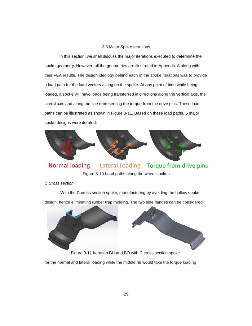
3.3 Major Spoke Iterations

In this section, we shall discuss the major iterations executed to determine the

spoke geometry. However, all the geometries are illustrated in Appendix A along with

their FEA results. The design ideology behind each of the spoke iterations was to provide

a load path for the load vectors acting on the spoke. At any point of time while being

loaded, a spoke will have loads being transferred in directions along the vertical axis, the

lateral axis and along the line representing the torque from the drive pins. These load

paths can be illustrated as shown in Figure 3-11. Based on these load paths, 5 major

spoke designs were iterated.

C Cross section

With the C cross section spoke, manufacturing by avoiding the hollow spoke

design, hence eliminating rubber trap molding. The two side flanges can be considered

for the normal and lateral loading while the middle rib would take the torque loading

Figure 3-10 Load paths along the wheel spokes

Figure 3-11 Iteration BH and BO with C cross section spoke

30

Semi Hexagonal cross section

The semi-hexagonal section is a modified C-cross section spoke with the two

edges joining the middle rib and the flanges are chamfered. The chamfer with 45° angle

gives a shape similar to half of a hexagon. The angular profile adds to the stiffness of the

structure and improves the draft angle for mold release.

T-cross section

The T-section spoke was made of two flanges, one flange in the wheel plane and

another flange bisecting perpendicularly to the first. The advantage was a relatively

simple lay-up compared to the above two cross sections and lesser weight. However, the

stiffness was poor resulting in more wheel deflection which is unfavorable.

Figure 3-12 Iterations BJ and BM showing semi-hexagonal sections

Figure 3-13 Iteration BP with the T-cross section wheel spoke

31

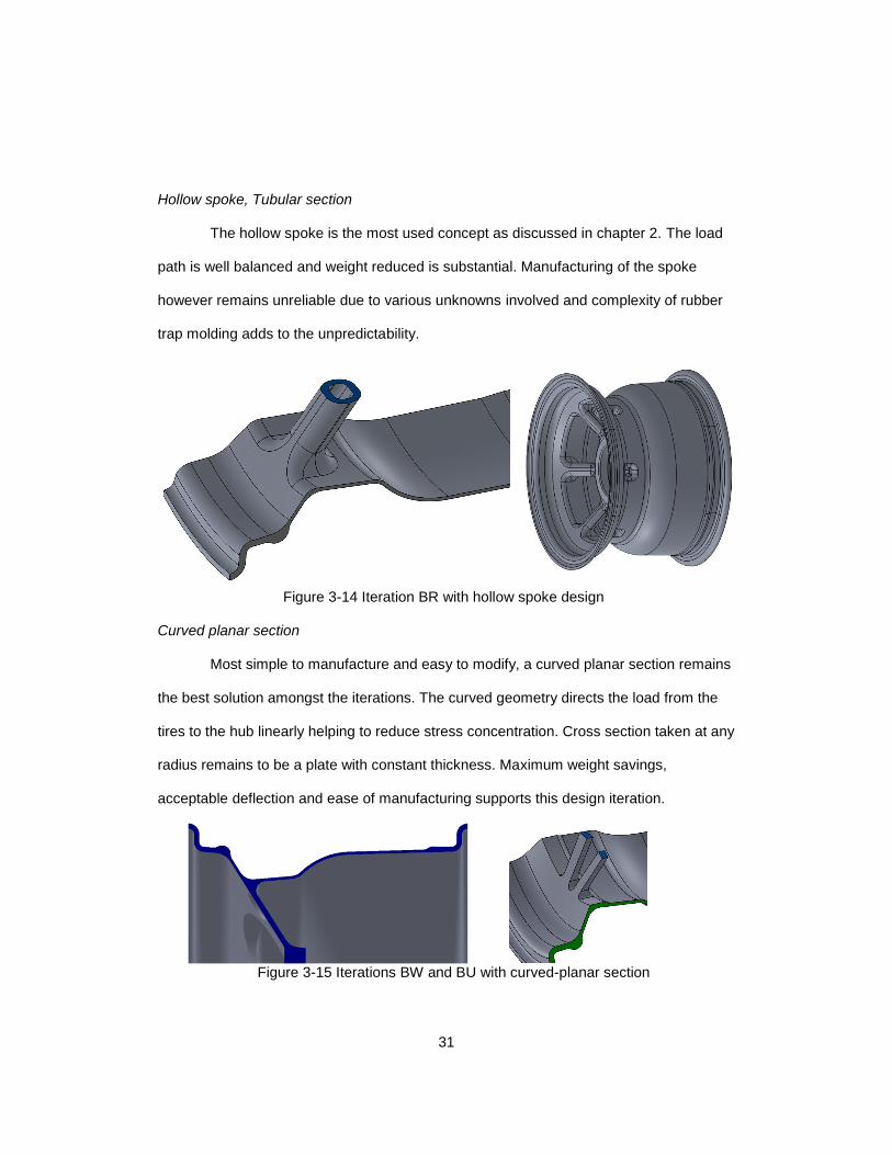
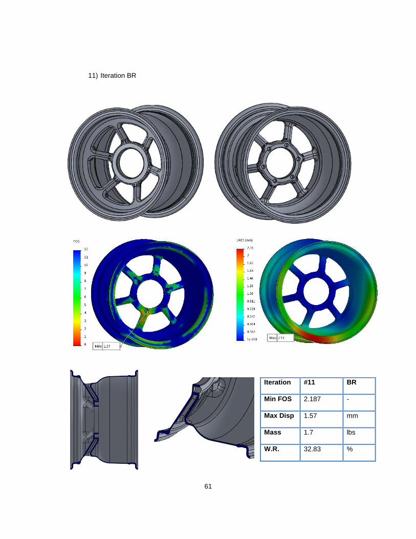
Hollow spoke, Tubular section

The hollow spoke is the most used concept as discussed in chapter 2. The load

path is well balanced and weight reduced is substantial. Manufacturing of the spoke

however remains unreliable due to various unknowns involved and complexity of rubber

trap molding adds to the unpredictability.

Curved planar section

Most simple to manufacture and easy to modify, a curved planar section remains

the best solution amongst the iterations. The curved geometry directs the load from the

tires to the hub linearly helping to reduce stress concentration. Cross section taken at any

radius remains to be a plate with constant thickness. Maximum weight savings,

acceptable deflection and ease of manufacturing supports this design iteration.

Figure 3-14 Iteration BR with hollow spoke design

Figure 3-15 Iterations BW and BU with curved-planar section

32

Chapter 4

Finite Element Analysis

As discussed earlier, the FEA was carried out in 2 stages to maximize the benefit

of iterative study on SolidWorks, and later a ply based analysis was carried out in

HyperWorks. The FEA setup remained the same for both the stages, however, in

HyperWorks, the geometry used was “Ply Based” taking into account the laminate layup

and fiber orientation. The bench mark comparison was made with respect to the 10”

Aluminum CF composite wheel.

4.1SolidWorks iteration

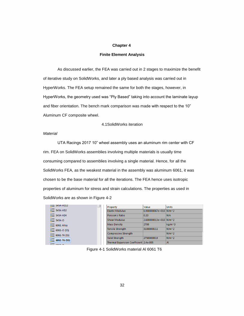
Material

UTA Racings 2017 10” wheel assembly uses an aluminum rim center with CF

rim. FEA on SolidWorks assemblies involving multiple materials is usually time

consuming compared to assemblies involving a single material. Hence, for all the

SolidWorks FEA, as the weakest material in the assembly was aluminum 6061, it was

chosen to be the base material for all the iterations. The FEA hence uses isotropic

properties of aluminum for stress and strain calculations. The properties as used in

SolidWorks are as shown in Figure 4-2

Figure 4-1 SolidWorks material Al 6061 T6

33

Setup

In FSAE dynamic events, the racecar is estimated to be around the corners for

most of its runs. Hence, a cornering scenario was decided to be analyzed. The 2017

racecar experiences a maximum of 2Gs lateral loading and a 3G normal load during high

speed of cornering with bump. This would account for maximum realistic loads that would

be transferred from the tires to the suspension components.

Fixed Geometry

As the loads are transferred from the tires to the hub, the hub mating surface is

assumed to be rigid. This corresponds to zero displacement of the reference surface. The

drive pin holes are given fixed geometry constrained to prevent rotation of the wheel. This

setup assumes the hub to be of infinite stiffness as the hub design is out of scope for this

project. Also, this assumption will result in safe design of the wheel which is ultimately

one of the objectives of this project.

External Loads

The external loads were based on the scenario as described in the setup section

of this chapter. As per UTA Racing’s proprietary load calculator spreadsheet, a 1000lbf

Figure 4-3 Fixed geometry for drive pins Figure 4-2 Zero displacement of hub contact surface

34

normal load and a 650lbf lateral load acts at the contact patch on the vehicle for the

cornering scenario as previously. This load is remotely applied on lower 60° of the wheel

lip and bead surface to simulate the load going through a single spoke. The remote load

source is taken at the midpoint of the contact patch. An illustration of the applied load is

shown in Figure 4-4

A compressive load of 2600lbf in total was applied on the lock nut and hub faces

equal in magnitude but opposite in direction to simulate the clamping force.

Figure 4-4 Remote load application

Figure 4-5 Clamping force on inboard and outboard

35

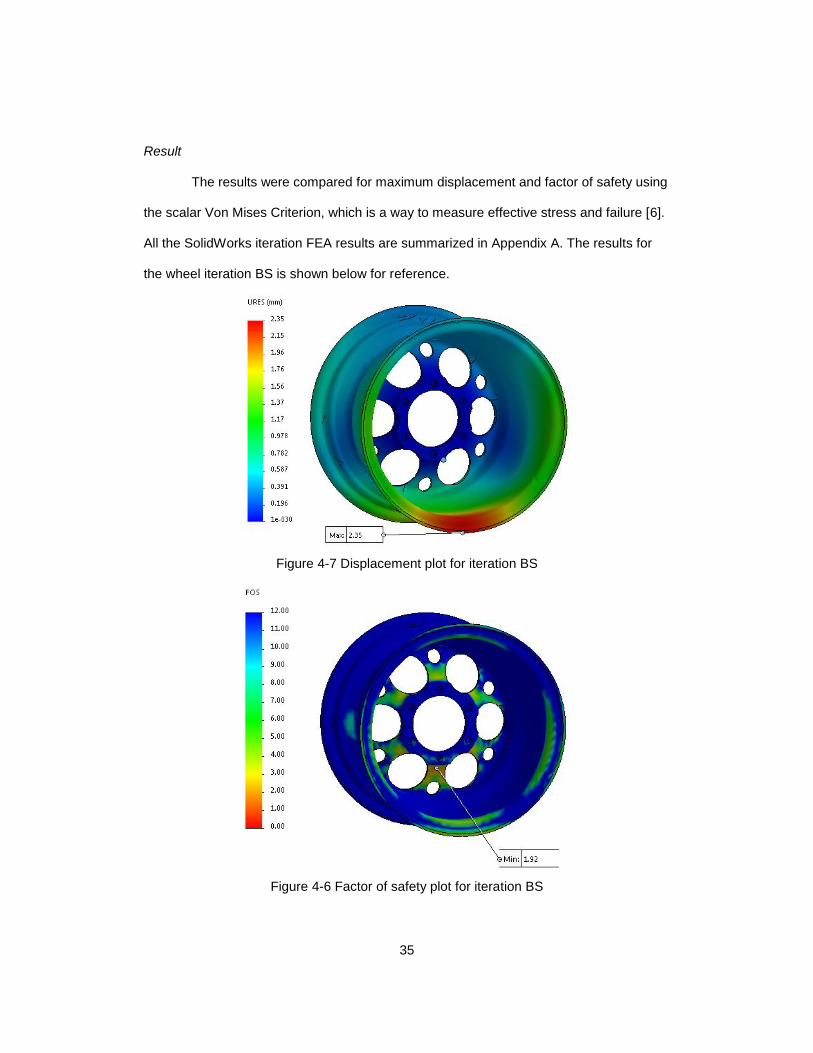
Result

The results were compared for maximum displacement and factor of safety using

the scalar Von Mises Criterion, which is a way to measure effective stress and failure [6].

All the SolidWorks iteration FEA results are summarized in Appendix A. The results for

the wheel iteration BS is shown below for reference.

Figure 4-6 Factor of safety plot for iteration BS

Figure 4-7 Displacement plot for iteration BS

36

4.2 Comparative study of SolidWorks iterations

To determine the design with least weight and acceptable deflection, a

comparison study was conducted. The comparison parameter were Factor of safety,

Mass, and Factor of safety per unit mass. The displacement values were comparable and

within 0.0025” of the existing design, hence it wasn’t considered in the comparative

study. Figure 4-8 shows a plot of the compared parameters for each iteration

The iteration considered to be ideal was the BS iteration. Although BV had most

FOS per unit mass, the mass savings were more on the BS while FOS requirement were

better than the F17 design. Since the objective was to achieve maximum weight

reduction, BS was more promising than BV and hence it was chosen for the detailed “ply-

based” FEA using HyperWorks

0.00

0.50

1.00

1.50

2.00

2.50

3.00

3.50

BH BI BJ BK BL BM BN BO BP BQ BR BS BT BU BV BW F-17

Iteration number

FOS and Mass relation

Factor of safety Mass (lbs) FOS per unit Mass

Figure 4-8 Comparative study of iterations

37

4.3 HyperWorks

HyperWorks is a CAE tool comprising of Hypermesh, OptiStruct, Radioss and

various other features. These features enable the use of Ply Based Modelling and

Analysis. Ply based analysis facilitates FEA in terms of individual laminate and plies. It

considers the particular stacking sequence and orientation of individual laminate helping

in increasing accuracy of the composite analysis.

HyperWorks uses the Tsai-Wu criterion [1] to determine composite failure which

for an orthotropic lamina considers failure in six-dimensional stress space. The Tsai Wu

criterion is more of general character as it uses an additional co-efficient for tensor

failure. One of the advantages of this criterion is that it uses symmetry properties which

are comparable to the stiffness and compliance properties. The Tsai-Wu criterion is

therefore widely used for industry applications.

Surface Model Generation

In order to get the laminate stack up accurate, a surface model is required to

provide continuity between each ply. This was created in SolidWorks using the surfaces

add in. A center line as shown in Figure for the geometry is selected and revolved as a

single surface.

Figure 4-9 Center line geometry for surface generation

38

The wheel center patterns are then projected onto the surface using the ‘Split

line’ tool and the surfaces are then trimmed. The surface as shown in Figure 4-10 is then

exported to a STEP file for compatibility with HyperWorks

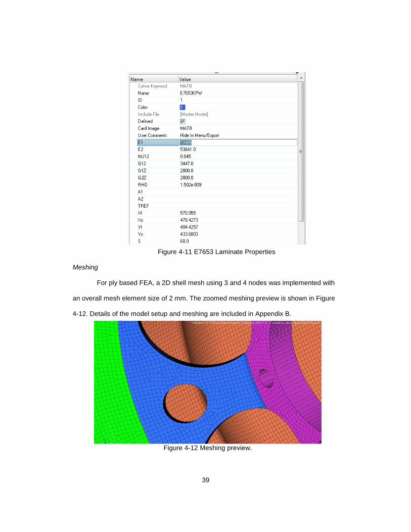
Material properties

The wheel material was considered with a foresight of availability of carbon fiber

for the UTA Racing team in the future. Hence, the material options were limited to the

current inventory of CF laminates the team had. Based on these considerations, the

material for the analysis was selected to be a Plain Weave T300 3KPW/E765 provided by

‘TORAY’. The epoxy used is a standard G94M also provided by ‘TORAY’. The

HyperWorks model has been updated to show all the CF laminates available at UTA

Racing. Figure 4-11 shows the material properties used in HyperWorks as obtained from

AGATE[19]

Figure 4-10 Surface model preview with cross section

39

Meshing

For ply based FEA, a 2D shell mesh using 3 and 4 nodes was implemented with

an overall mesh element size of 2 mm. The zoomed meshing preview is shown in Figure

4-12. Details of the model setup and meshing are included in Appendix B.

Figure 4-11 E7653 Laminate Properties

Figure 4-12 Meshing preview.

40

Ply orientation

The ply orientation is the most important factor while setting up a Ply Based FEA

model. The plies are oriented in the laminate to achieve a balanced laminate. The

primary angles considered were 0°, ±45° and ±90° [4]. Figure 4-13 shows the ply

orientation for the outboard wheel center pattern which uses 0° and ±45° ply orientations.

The ply orientation needs to be modified for each laminate material change based on the

fiber’s properties in each direction.

The ply layup is based on the actual model to match the thickness as designed.

The plies range from a minimum of 10 plies for areas with 2 mm thickness, 18 plies for

zones with 3.6 mm thickness and 73 plies for the hub mounting center. A cross section of

the ply model is shown in Figure 4-14.

Figure 4-13 Ply orientation for wheel center

41

Setup

Both SolidWorks and OptiStruct models use the same FEA setup and loads. The

constraints used for drive pins is fixed around each axis while the hub mating surface is

constrained for any lateral motion. The loads of 650lbf and 1000lbf in lateral direction and

normal directions respectively are acted upon the lower 60° of the model.

Results

The results obtained were plot for carbon failure and displacement. The carbon

failure gives us the reliability of the ply geometry and bond strength. Figure 4-15 and

Figure 4-14 Cross section with ply distribution

42

Figure 4-16 show the carbon failure plot and displacement plots which are within the

constraints of the design

Figure 4-15 Composite Failure

Figure 4-16 Max dispacement

43

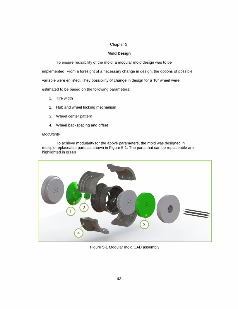
Mold Design

To ensure reusability of the mold, a modular mold design was to be

implemented. From a foresight of a necessary change in design, the options of possible

variable were enlisted. They possibility of change in design for a 10” wheel were

estimated to be based on the following parameters:

1. Tire width

2. Hub and wheel locking mechanism

3. Wheel center pattern

4. Wheel backspacing and offset

Modularity

To achieve modularity for the above parameters, the mold was designed in multiple replaceable parts as shown in Figure 5-1. The parts that can be replaceable are highlighted in green

Figure 5-1 Modular mold CAD assembly

1 2

3

4

44

The part 1 is called the wheel center pattern mold. It is designed for the weight

reduction pattern lay-up. In future, due to change vehicle design, if the loads on the wheel

increase or decrease, simply replacing this mold piece can help modify the wheel design.

Part 2 also called as the ‘center piece’ is for the lock nut spacing. Having an

independent center piece will allow to opt for lug-nut based attachment.

Part 3 is called as the ‘Width mold’ determines the width of the wheel. Changing

its length along the axis may give wheels of different widths ranging from 6” to 8”. The

wheel offset and backspacing can be adjusted by using various combinations of different

2nd and 3rd parts.

The 4th part is the clamp shell which may change in case of a change in width.

Only part 4 shall be made of CF while others are all aluminum components. The entire

mold assembly apart from the clamp shells are secured using 6 numbers of ¼” studs and

a ½” stud all secured with metallic lock nuts.

Mold design in SolidWorks

All the mold profiles are generated from the parametric sketch designed in

SolidWorks. This allows to maintain dimensional accuracy of the part. An efficient way to

design the wheel center mold referred to as Part 1 in Figure 5-1 is to use the ‘Combine’

feature in SolidWorks.

Figure 5-2 Wheel center mold model tree

45

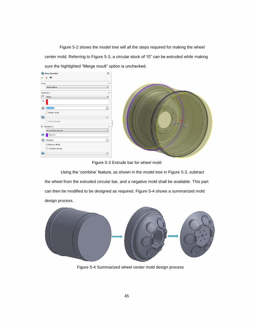
Figure 5-2 shows the model tree will all the steps required for making the wheel

center mold. Referring to Figure 5-3, a circular stock of 10” can be extruded while making

sure the highlighted “Merge result” option is unchecked.

Using the ‘combine’ feature, as shown in the model tree in Figure 5-3, subtract

the wheel from the extruded circular bar, and a negative mold shall be available. This part

can then be modified to be designed as required. Figure 5-4 shows a summarized mold

design process.

Figure 5-3 Extrude bar for wheel mold

Figure 5-4 Summarized wheel center mold design process

46

Draft analysis

As considered during iterative study, the draft analysis on the mold is also

checked for any interfering bodies. The parts concerned primarily for the draft analysis

are the outboard and inboard components of the wheel center mold, and the clamp

shells, analysis of which are shown below. These molds were found to fulfil the

necessary draft angles.

Figure 5-5 Draft analysis on mold components

Wheel Center outboard

mold

Wheel Center inboard

mold

Wheel outer

mold

Clamp shell

47

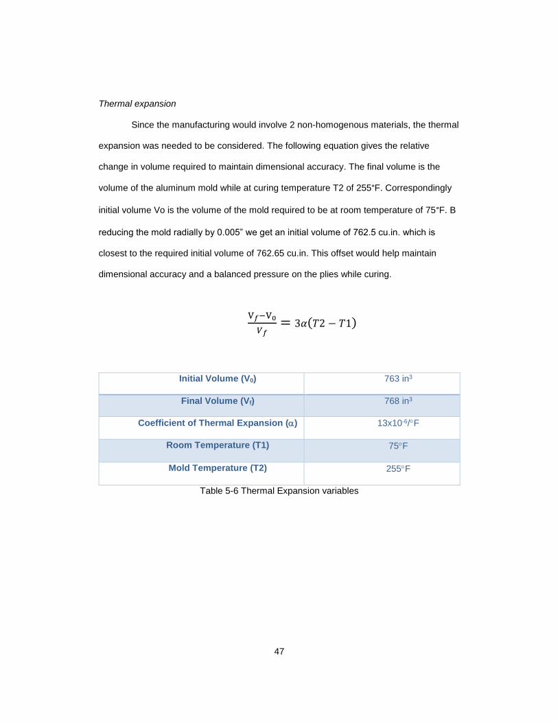
Thermal expansion

Since the manufacturing would involve 2 non-homogenous materials, the thermal

expansion was needed to be considered. The following equation gives the relative

change in volume required to maintain dimensional accuracy. The final volume is the

volume of the aluminum mold while at curing temperature T2 of 255°F. Correspondingly

initial volume Vo is the volume of the mold required to be at room temperature of 75°F. B

reducing the mold radially by 0.005” we get an initial volume of 762.5 cu.in. which is

closest to the required initial volume of 762.65 cu.in. This offset would help maintain

dimensional accuracy and a balanced pressure on the plies while curing.

V𝑓−V0

𝑉𝑓= 3𝛼(𝑇2 − 𝑇1)

Initial Volume (V0) 763 in3

Final Volume (Vf) 768 in3

Coefficient of Thermal Expansion () 13x10-6/F

Room Temperature (T1) 75F

Mold Temperature (T2) 255F

Table 5-6 Thermal Expansion variables

48

Conclusion and Future Scope

The designed wheel with an estimated weight of 1.8 lbs demonstrates 29%

weight reduction on the existing design weighing 2.5 lbs thus achieving the first objective

of achieving a minimum of 15% weight reduction. The maximum displacement of 2.8 mm

for the carbon wheel is comparable with the 2.95 mm displacement as seen in the

existing design. The modular mold designed enables future improvements to the design,

which is parametrically modelled for ease of modification. The advantage of reduction in

manufacturing time and cost by elimination of the aluminum wheel center makes the

wheel design adaptable for the future FSAE racecars designed by UTA Racing. All these

factors suggest the project has been successfully achieved its targets.

There is however, a major scope of improvement. The hub mating surface is

currently designed to take 73 plies resulting in unnecessary stiffness and weight of the

center section. It is highly suggested that this section be reduced in thickness while a

slight modification on the hub length shall be necessary. The advantage would be further

reduction in unsprung mass and hence rotational moment of inertia, while saving

expensive carbon fiber resources.

49

Appendix A

SolidWorks Iteration Illustrations

50

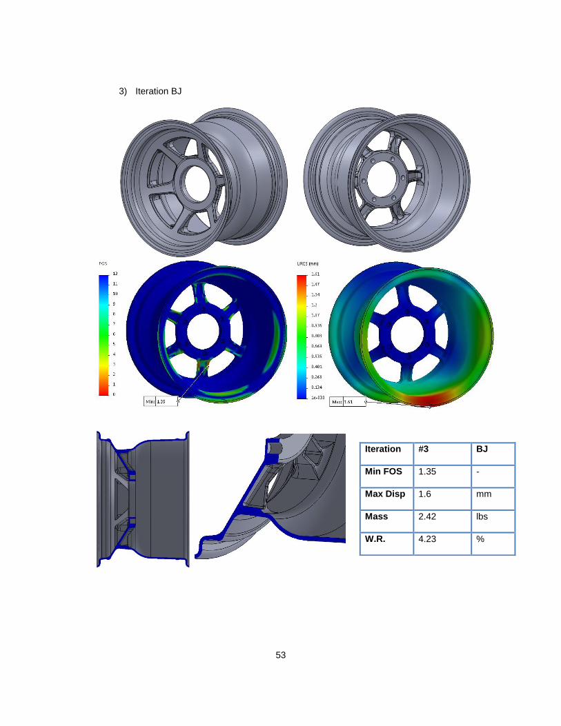
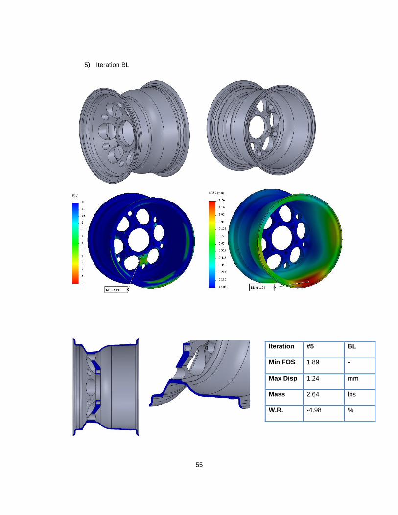
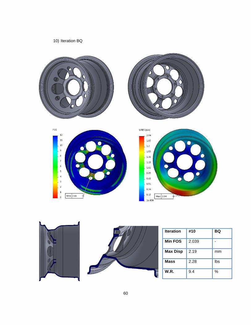
This appendix consists of illustrations and simulation results of the iterative study

performed in SolidWorks. Each page has the design geometry on top, followed by FEA results

with Factor of safety on the left and displacement plot on the right. The bottom row shows the

cross-section geometry along with a summarized specification of the iterated design.

51

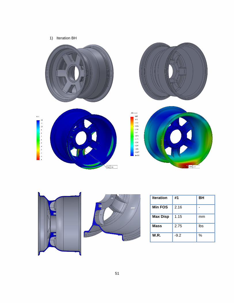
1) Iteration BH

Iteration #1 BH

Min FOS 2.16 -

Max Disp 1.15 mm

Mass 2.75 lbs

W.R. -9.2 %

52

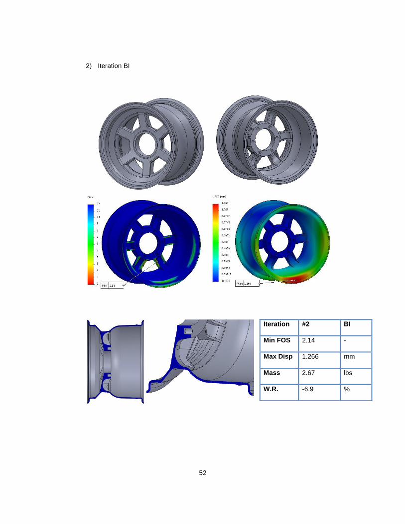
2) Iteration BI

Iteration #2 BI

Min FOS 2.14 -

Max Disp 1.266 mm

Mass 2.67 lbs

W.R. -6.9 %

53

3) Iteration BJ

Iteration #3 BJ

Min FOS 1.35 -

Max Disp 1.6 mm

Mass 2.42 lbs

W.R. 4.23 %

54

4) Iteration BK

Iteration #4 BK

Min FOS 1.59 -

Max Disp 1.58 mm

Mass 2.40 lbs

W.R. 4.79 %

55

5) Iteration BL

Iteration #5 BL

Min FOS 1.89 -

Max Disp 1.24 mm

Mass 2.64 lbs

W.R. -4.98 %

56

6) Iteration BM

Iteration #6 BM

Min FOS 1.42 -

Max Disp 2.51 mm

Mass 1.71 lbs

W.R. 32.42 %

57

7) Iteration BN

Iteration #7 BN

Min FOS 0.96 -

Max Disp 2.72 mm

Mass 2.34 lbs

W.R. 7.15 %

58

8) Iteration BO

Iteration #8 BO

Min FOS 2.03 -

Max Disp 1.24 mm

Mass 2.25 lbs

W.R. 10.66 %

59

9) Iteration BP

Iteration #9 BP

Min FOS 2.181 -

Max Disp 1.21 mm

Mass 2.25 lbs

W.R. 10.69 %

60

10) Iteration BQ

Iteration #10 BQ

Min FOS 2.039 -

Max Disp 2.19 mm

Mass 2.28 lbs

W.R. 9.4 %

61

11) Iteration BR

Iteration #11 BR

Min FOS 2.187 -

Max Disp 1.57 mm

Mass 1.7 lbs

W.R. 32.83 %

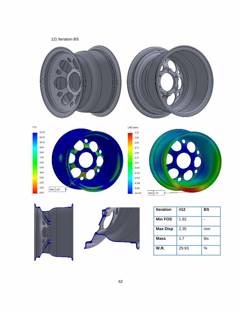
62

12) Iteration BS

Iteration #12 BS

Min FOS 1.92 -

Max Disp 2.35 mm

Mass 1.7 lbs

W.R. 29.93 %

63

13) Iteration BT

Iteration #13 BT

Min FOS 2.306 -

Max Disp 1.86 mm

Mass 1.8 lbs

W.R. 28.91 %

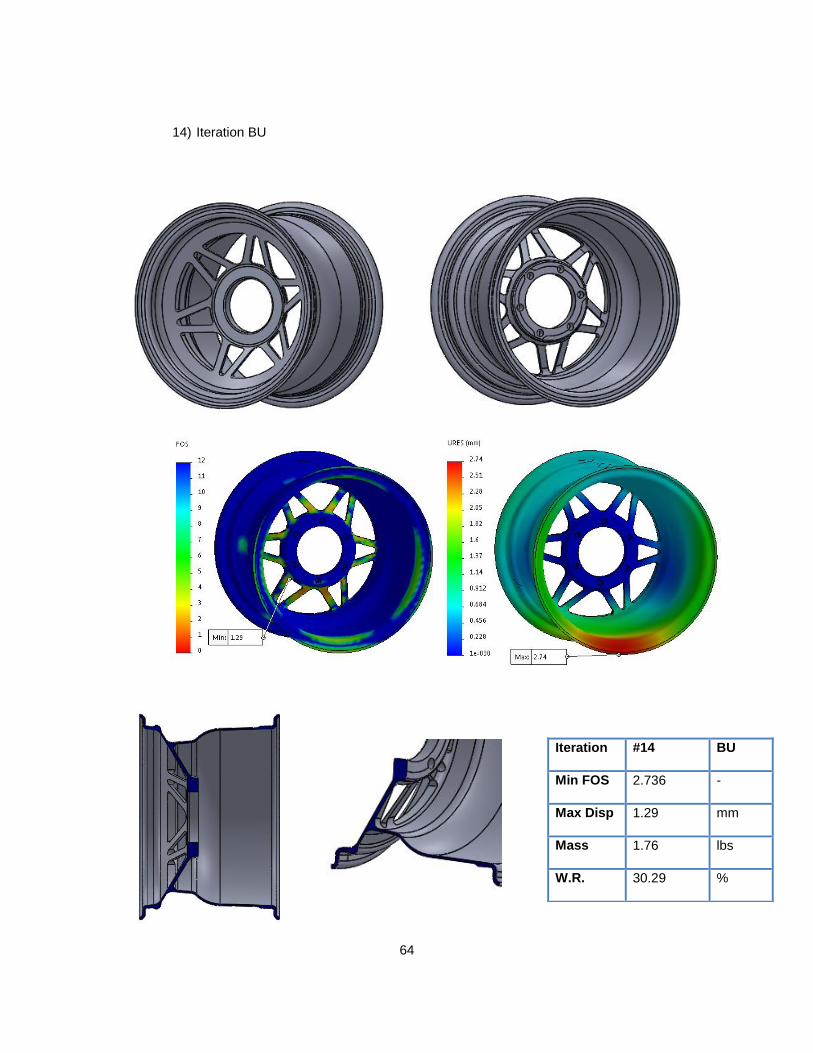
64

14) Iteration BU

Iteration #14 BU

Min FOS 2.736 -

Max Disp 1.29 mm

Mass 1.76 lbs

W.R. 30.29 %

65

15) Iteration BV

Iteration #15 BV

Min FOS 2.96 -

Max Disp 1.578 mm

Mass 1.99 lbs

W.R. 21.15 %

66

16) Iteration BW

Iteration #16 BW

Min FOS 1.1 -

Max Disp 2.27 mm

Mass 1.85 lbs

W.R. 26.78 %

67

Summary table:

# Iteration DISP FOS MASS(LBS) W.R. % FOS/Mass(lbs)

1 BH 1.148 2.16 2.75 -9.20 0.786

2 BI 1.266 2.14 2.67 -6.19 0.801

3 BJ 1.605 1.35 2.40 4.83 0.563

4 BK 1.582 1.59 2.40 4.79 0.662

5 BL 1.42 2.26 2.64 -4.98 0.855

6 BM 2.511 1.42 1.71 32.42 0.829

7 BN 2.721 0.96 2.34 7.15 0.410

8 BO 2.033 1.24 2.25 10.66 0.552

9 BP 2.181 1.21 2.25 10.69 0.535

10 BQ 2.039 2.19 2.28 9.40 0.959

11 BR 2.187 1.57 1.70 32.83 0.925

12 BS 2.343 1.94 1.77 29.93 1.094

13 BT 2.306 1.86 1.80 28.81 1.033

14 BU 2.736 1.29 1.76 30.29 0.732

15 BV 1.572 2.96 1.99 21.15 1.487

16 BW 2.119 1.35 1.85 26.78 0.732

F-17 2.408 1.66 2.52 0.00 0.659

68

Appendix B

HyperWorks guide

69

The purpose of Appendix B is to provide a guide to setup and trouble shoot the ply

based wheel model. Although major steps have been included in this guide, some errors may

occur due to hardware issues. These errors are usually resolvable by referring to the Altair

Helpdesk online. Let us proceed with the modelling and FEA setup.

The first step of the analysis is to import the supported model file. As we are

going to work with composite layup, we would be using a CAD model made up of

surfaces.

To import the mode, go to IMPORT MODEL option located on the toolbar just

below the task bar. Then select IMPORT GEOMETRY. In the import geometry menu,

browse to the location of the file and select it.Make sure to select the file type from the

file type drop box. We are using STEP format CAD file for our FEA.

The next important step before finishing the import process is to convert the unit

system if required. As we are going to use the SI unit system, Hyperworks default SI

system units are mm, N, Tons and seconds. If the model is made up in English units.

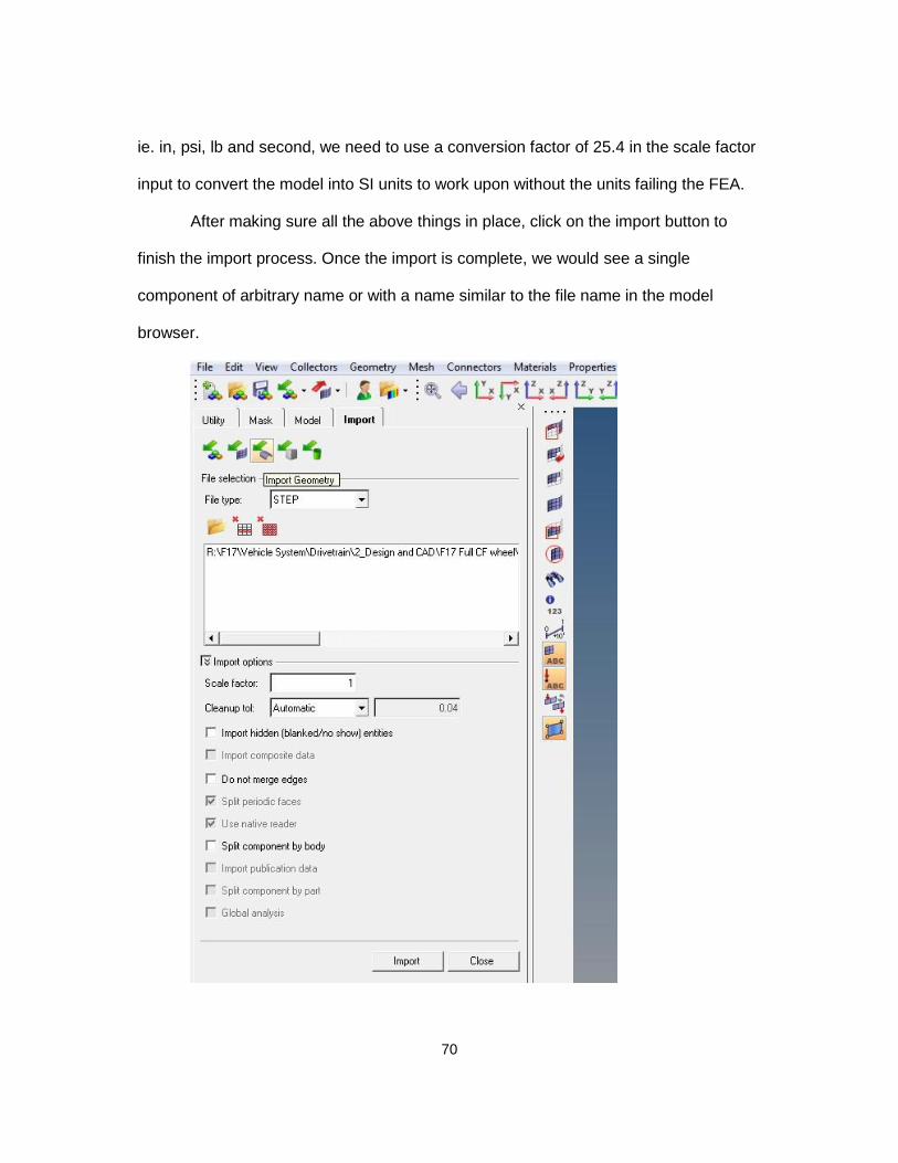
70

ie. in, psi, lb and second, we need to use a conversion factor of 25.4 in the scale factor

input to convert the model into SI units to work upon without the units failing the FEA.

After making sure all the above things in place, click on the import button to

finish the import process. Once the import is complete, we would see a single

component of arbitrary name or with a name similar to the file name in the model

browser.

71

Component Creation -

The next step is to create components. We would create components equal to the number of

regions the wheel is divided into. To do so, click on the components tool button on the toolbar just below

the graphic window. Give the desired name and select no card image and no property.

We have defined 4 components in our model for the wheel’s ply layup and 1 component to define

the remoteload from the contact patch on the wheel.

72

Geometry Editing –

The next step is to move the various surfaces to their respective components

for the esae of meshing and layup.

To do so, we use the organize tool. Go to the Tool toolbar and click on organize

buton. Then using the toggle button next to the green box, select surfaces. This enables us to

move the surfaces to desired components created earlier.

Next, select the surfaces needed to be moved and then click on the dest

component= option to select the destination component. To finish moving the components, click

on move command. Do this process multiple times untill all our surfaces are defined in the

corresponding components.

73

74

Material Definition –

We now create the material which we would apply to our composite laminate.

Click on the material toll on the tollbar below the graphic window. Define the name of the

material, select type as orthotropic and card image as MAT8 and click on create.

Locate the material in the model browser and click on it to display the edit

window below the model browser. Enter the material properties as shown in the image below.

75

Property Definition –

The next step is to define the properties for the material. A general rule of thumb is

followed which states “Number of Properties = Number of components” except the component

for rigid element which don’t always need a property definition.

To create a property, click on the properties tool on the tollbar below the graphic

window and define the name needed. Select type as 2D and card image as PCOMPP and click

create to finish creating a property.

Now go to the model browser and click on the property created to check for 2D,

PCOMPP and change the SB and FT values to 60.0 and STRN respectively for all properties

created.

76

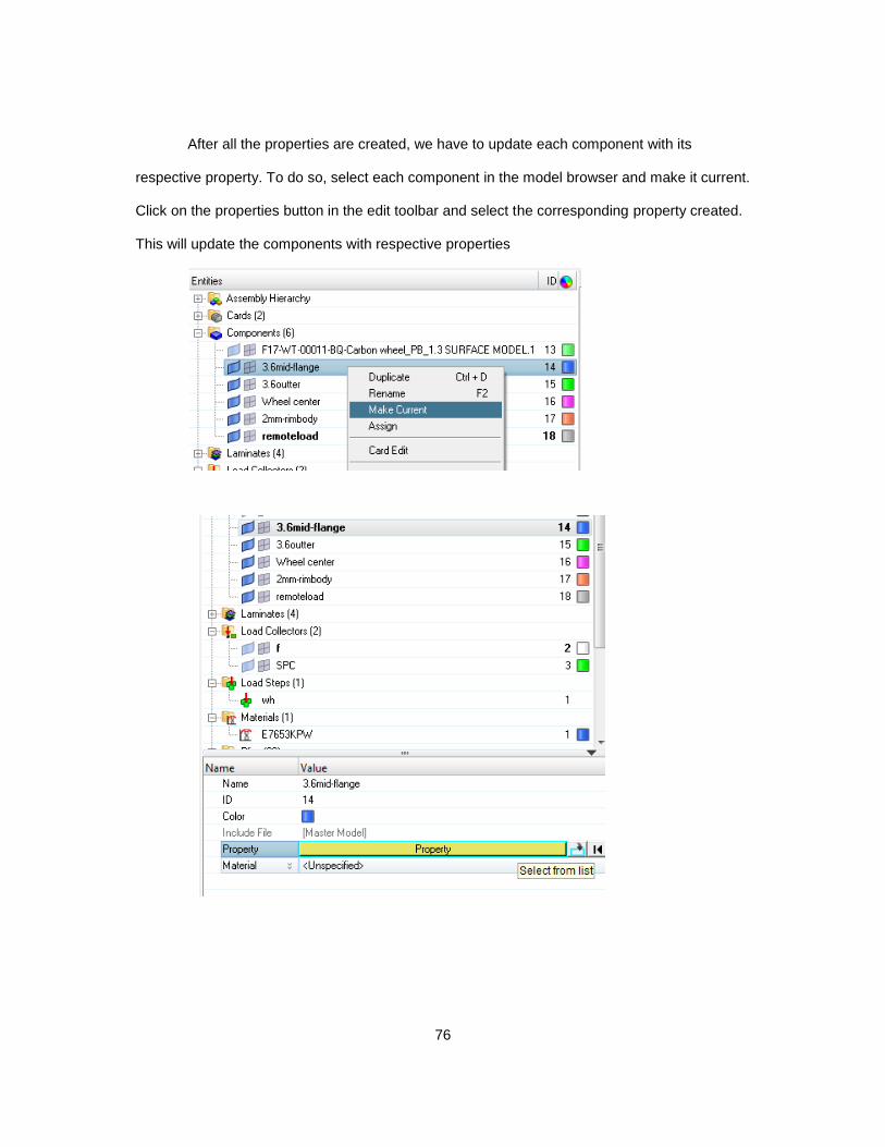
After all the properties are created, we have to update each component with its

respective property. To do so, select each component in the model browser and make it current.

Click on the properties button in the edit toolbar and select the corresponding property created.

This will update the components with respective properties

77

select the corresponding property and click ok

Before starting the preprocessing, surface connectivity checks need to be performed

Geometry Editing –

Make sure the wireframe geometry is visible and then go to geom tool bar.

Select surface edit option. This will show the surfaces in 3 colors. We have to make sure that

the interconnecting surfaces should not be red in color which means discontinuity.

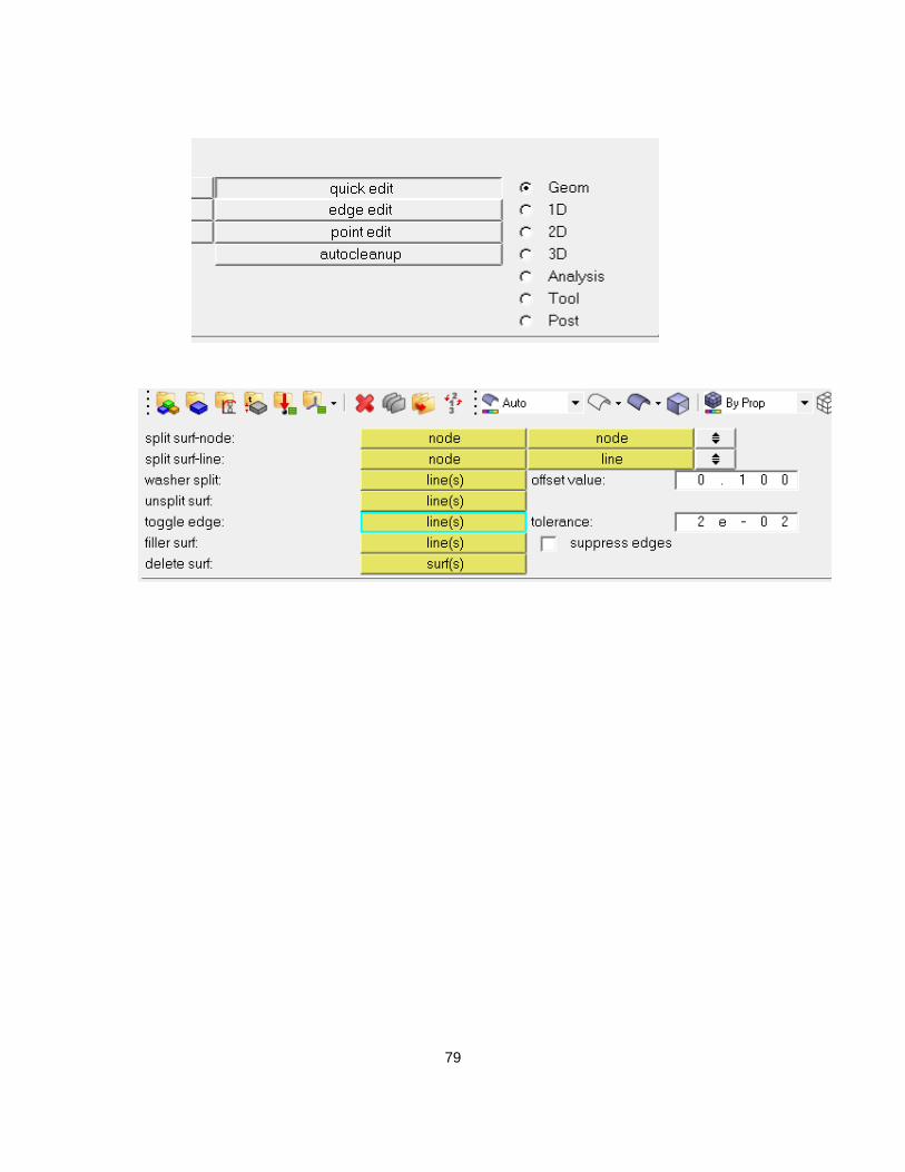
If any such surfaces are found, go to the geom tab and click on quick edit.

Select the toggle edge option and lick on the edge that is red in color. This will stitch the edges

together and allow for connectivity.

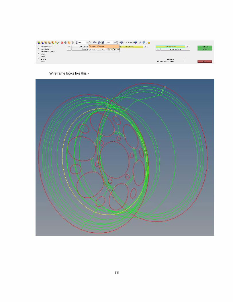
78

Wireframe looks like this -

79

80

Meshing –

Once the geometry is fixed and finalized along with the component, material

and property definition, the next step is to define the mesh for each component. We use 2D

elements to mesh our model as we are working with composites and surface based geometry

Goto 2D and select automesh. Select element size to desired value. Remember to have

the components selected as current as described earlier. Also, the elements selection option

should be “elems to current comp”. After making sure the below highlighted options are correct,

click on mesh. Repeat the steps by making current every component and then mesh.

81

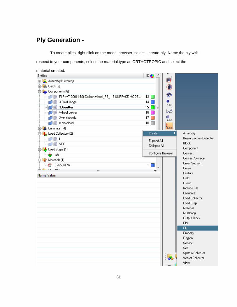
Ply Generation -

To create plies, right click on the model browser, select—create-ply. Name the ply with

respect to your components, select the material type as ORTHOTROPIC and select the

material created.

82

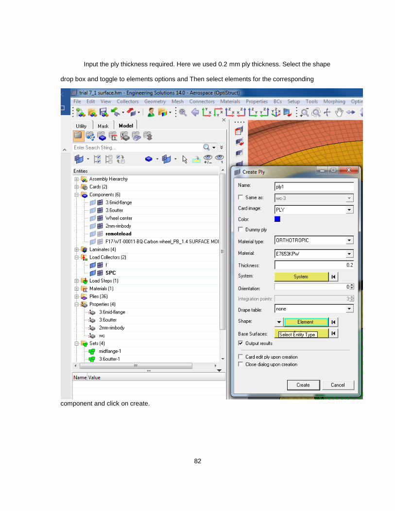
Input the ply thickness required. Here we used 0.2 mm ply thickness. Select the shape

drop box and toggle to elements options and Then select elements for the corresponding

component and click on create.

83

After the first ply is defined for each component, a SET gets automatically created

containing all the elements of that corresponding components in the model browser.

84

We have to create multiple number of plies for the same components as the depending

on the final size of the component. To this and save time, we use the duplicate option to create

desired number of plies for a particular component and do the same for other component as

well. Then we change the orientation for each ply from the model browser to 0,45,-45 and 0 as

required and in the order of the stacking sequence.

85

The next step is to define the entity set for each ply that’s duplicated. To do so we

select all the plies of the same component, right click and go to edit option. Here we select the

update shape option and select set from the drop box.

Then we select the set related to our desired component and select update.

Repeat this process to update all the plies that are present. After the Plies are defined,

we create LAMINATE for each component which defines the STACKING SEQUENCE.

86

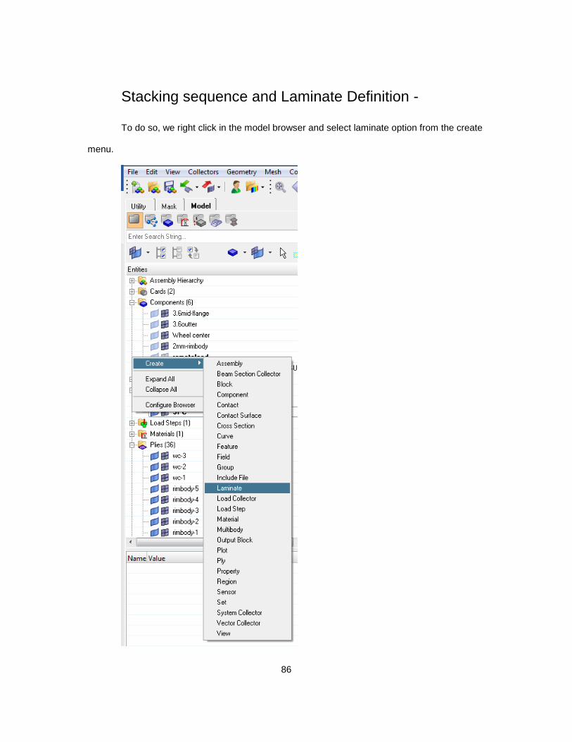
Stacking sequence and Laminate Definition -

To do so, we right click in the model browser and select laminate option from the create

menu.

87

A create laminate window appears where we give the desired name for the laminate

and select SYMMETRIC SMEAR as the laminate option.

Then we select the plies in the stacking order we want. We have followed the order of

0,45,0,-45,0 and so on and click create.

Do this for the number of components you have created.

NOTE : -

The number of plies to be created depends on the stacking option.

If total of 18 plies are required for a component, then create 18 plies if only SMEAR

property is going to be used in the stacking sequence and if using the SYMMETRIC SMEAR,

88

then only 9 plies are required to be defined. The use of smear and symmetric smear depends

on the complexity of the model and if non-symmetric ply layup is needed. Also, using

SYMMETRIC SMEAR saves time in ply creation.

After all the laminates are defined, we go back to edit properties if the plies are not

dropped as desired.

To view the ply drop, we toggle the model view to “By Prop”, 2D element visualization to

2D detailed element view and toggle composite layers option to composite layers. This shows

the model the way it is stacked. Visually check the model for the ply drop and if the ply drop is

no on the desired side of the plane, go back to the corresponding property of the component

and change the Z0 OPTION to TOP, BOTTOM or REAL as required.

89

90

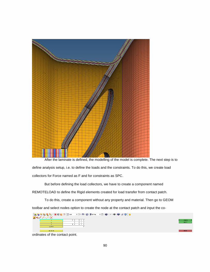
After the laminate is defined, the modelling of the model is complete. The next step is to

define analysis setup, i.e. to define the loads and the constraints. To do this, we create load

collectors for Force named as F and for constraints as SPC.

But before defining the load collectors, we have to create a component named

REMOTELOAD to define the Rigid elements created for load transfer from contact patch.

To do this, create a component without any property and material. Then go to GEOM

toolbar and select nodes option to create the node at the contact patch and input the co-

ordinates of the contact point.

91

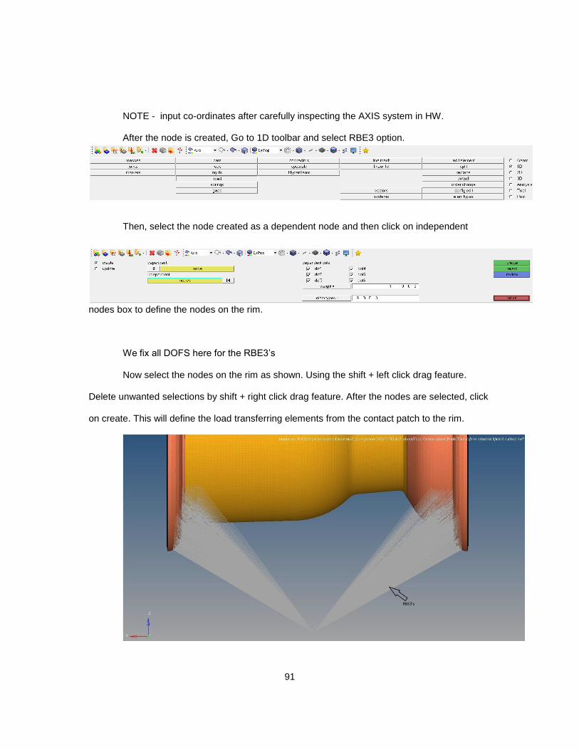
NOTE - input co-ordinates after carefully inspecting the AXIS system in HW.

After the node is created, Go to 1D toolbar and select RBE3 option.

Then, select the node created as a dependent node and then click on independent

nodes box to define the nodes on the rim.

We fix all DOFS here for the RBE3’s

Now select the nodes on the rim as shown. Using the shift + left click drag feature.

Delete unwanted selections by shift + right click drag feature. After the nodes are selected, click

on create. This will define the load transferring elements from the contact patch to the rim.

92

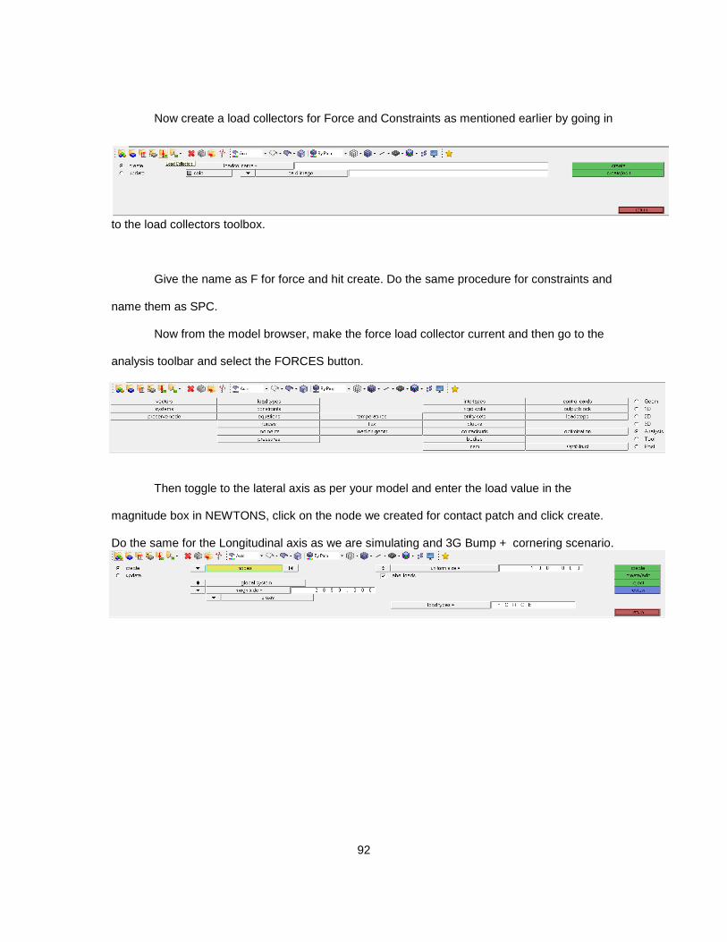
Now create a load collectors for Force and Constraints as mentioned earlier by going in

to the load collectors toolbox.

Give the name as F for force and hit create. Do the same procedure for constraints and

name them as SPC.

Now from the model browser, make the force load collector current and then go to the

analysis toolbar and select the FORCES button.

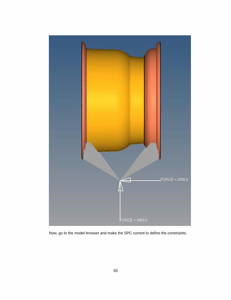
Then toggle to the lateral axis as per your model and enter the load value in the

magnitude box in NEWTONS, click on the node we created for contact patch and click create.

Do the same for the Longitudinal axis as we are simulating and 3G Bump + cornering scenario.

93

Now, go to the model browser and make the SPC current to define the constraints.

94

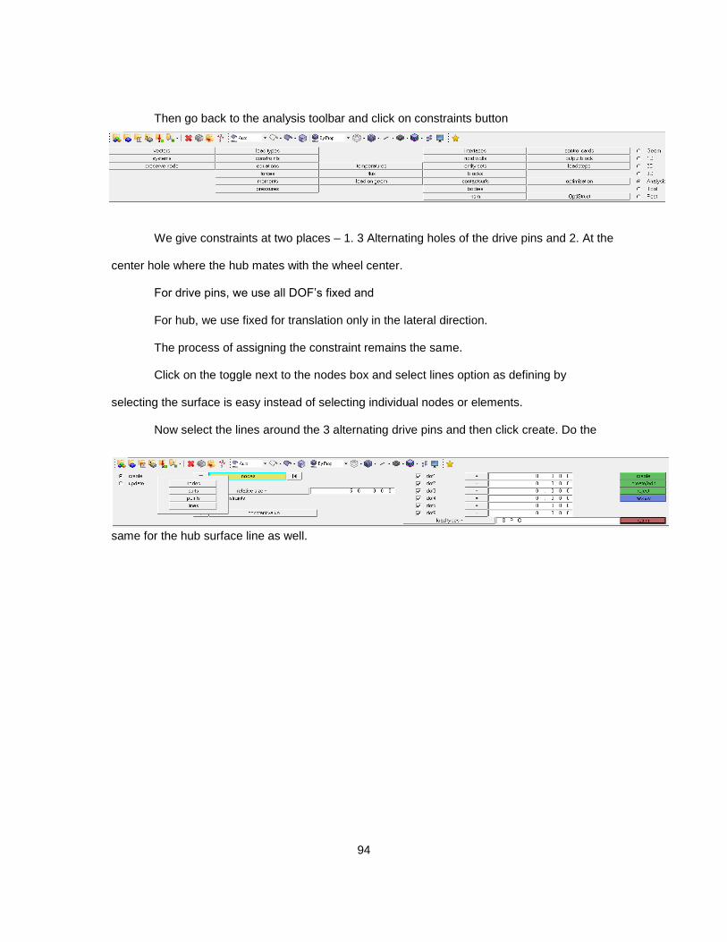
Then go back to the analysis toolbar and click on constraints button

We give constraints at two places – 1. 3 Alternating holes of the drive pins and 2. At the

center hole where the hub mates with the wheel center.

For drive pins, we use all DOF’s fixed and

For hub, we use fixed for translation only in the lateral direction.

The process of assigning the constraint remains the same.

Click on the toggle next to the nodes box and select lines option as defining by

selecting the surface is easy instead of selecting individual nodes or elements.

Now select the lines around the 3 alternating drive pins and then click create. Do the

same for the hub surface line as well.

95

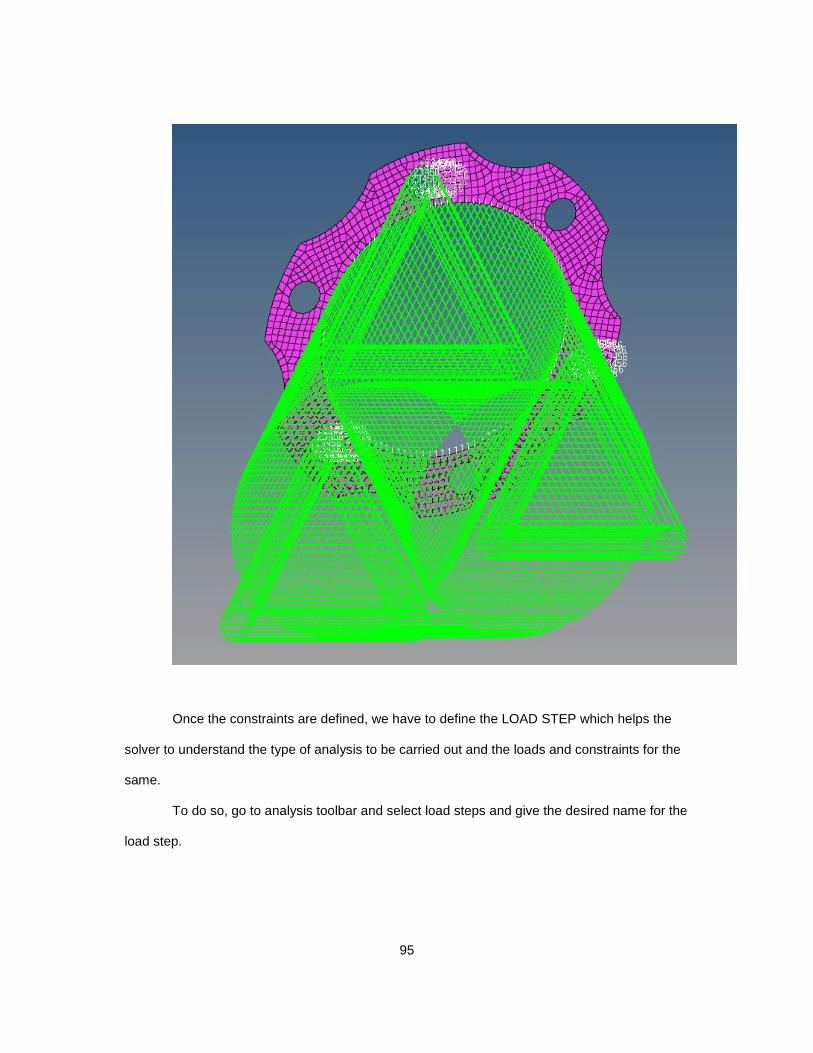
Once the constraints are defined, we have to define the LOAD STEP which helps the

solver to understand the type of analysis to be carried out and the loads and constraints for the

same.

To do so, go to analysis toolbar and select load steps and give the desired name for the

load step.

96

Select the type as Linear Static and check mark the spc and load option. Now go to spc option

and select the load collector SPC we created earlier and do the same for the load option. Then

hit the create button.

97

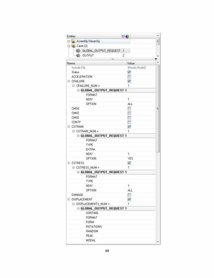
The next step is to define the output control cards as we want to see the ply failure which is not

a default output.

To do so, go to the analysis tollbar and click on control cards option.

Now navigate to GLOBAL_OUTPUT_REQUEST and click it.

Here select CSTAIN, CFAILURE and CSTRESS options.

Hit return to finish defining the control cards.

98

99

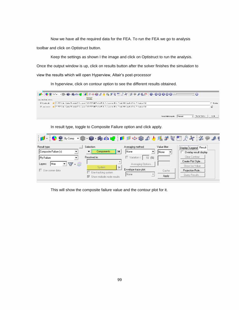
Now we have all the required data for the FEA. To run the FEA we go to analysis

toolbar and click on Optistruct button.

Keep the settings as shown I the image and click on Optistruct to run the analysis.

Once the output window is up, click on results button after the solver finishes the simulation to

view the results which will open Hyperview, Altair’s post-processor

In hyperview, click on contour option to see the different results obtained.

In result type, toggle to Composite Failure option and click apply.

This will show the composite failure value and the contour plot for it.

100

References

1. Robert M. Jones, Mechanics of composite materials, Virginia Polytechnic Institute

and State University, 1999.

2. Caroll Smith, Tune to Win, Aero Publishers Inc, 1978.

3. Douglas Milliken and William Milliken, Race car vehicle dynamics, SAE International,

1995.

4. P. Joyce, “PAX-Short course on laminates”, 2003.

5. Hans Walther, Development of a lightweight laminated composite wheel for Formula

sae race vehicle , ProQuest LLC, 2016.

6. John Edward Akin, Finite Element Analysis Concepts via SolidWorks , Rice

University, 2010.

7. http://hyperphysics.phy-astr.gsu.edu/hbase/icyl.html#icyl

8. http://hyperphysics.phy-astr.gsu.edu/hbase/mi.html

9. http://www.thecartech.com/subjects/auto_eng/car_performance_formulas.htm

10. https://www.slideshare.net/waqasrashidchaudhary/angularmotionrotationdynamics-

100212165341phpapp01

11. https://en.wikipedia.org/wiki/Unsprung_mass

12. https://www.afsrhuck.net/us/

13. http://www.ptc.com/cad-software-blog/parametric-vs-direct-modeling-which-side-are-

you-on

14. http://www.tyresizecalculator.com/wheels/wheel-rim-profiles

15. http://compositeslab.com/composites-manufacturing-processes/

16. https://i.ytimg.com/vi/hvwY4LCJLiE/maxresdefault.jpg

17. http://www.allfordmustangs.com/wordpress/wp-content/uploads/2015/11/CF-3.jpg

18. http://www.fsaeonline.com/content/2017-18%20FSAE%20Rules%209.2.16a.pdf

101

19. http://www.niar.wichita.edu/agate/

20. https://media.ford.com/content/dam/fordmedia/North%20America/US/2016/05/17/car

bon-wheels-fact-sheet.pdf

21. http://www.carbonrev.com/technology

22. https://www.youtube.com/watch?v=PGGiuaQwcd8

23. Tim Patek, Personal communication, 2016

24. Pratik Bhagwat and others, “Design of 10” carbon wheel mold”, internal ME 5358-

001, University of Texas, Arlington, 2016

102

Biographical Information

Pratik Ganesh Bhagwat is a Formula SAE enthusiast and a Mechanical Engineer

from University of Texas, Arlington. He was the Chassis Lead and Drivetrain design

engineer for UTA Racing in 2017 and was involved with 2 FSAE racing teams between

2013 to 2017 developing 4 FSAE racecars. He earned the Bachelor of Science degree in

Automotive Engineering in 2015 from the University of Mumbai, India while being the

Chief engineer for Hyperion Racing FSAE team. He holds the Master of Science degree

and a Graduate Certificate in Automotive Engineering from the University of Texas,

Arlington, from where he graduated in May 2017.

Throughout his engineering research, he concentrated on areas involving CAE,

Structural Mechanics, product design and development and automotive part design.

Through FSAE, he was involved in various projects, namely, Design of FSAE Chassis,

Design and manufacture of FSAE racecar Body, Design of Differential carrier,

Suspension Upright design, Structural Analysis of Drivetrain system of an Electric Race

car, Design and Analysis of High Voltage Accumulator container and many more.

Pratik aims to play a crucial role in motorsports as a design engineer. He is

looking forward for global opportunities in the Automotive industry.