1

Food Access and Food Choice: Applications for Food Deserts

Final Report

Research Innovation and Development Grants in Economics (RIDGE)

Grant # 59-5000-0-0014

Gayaneh Kyureghian

Research Assistant Professor

Department of Food Science and Technology

The Food Processing Center

University of Nebraska-Lincoln

Rodolfo M. Nayga, Jr.

Professor and Tyson Endowed Chair

Department of Agricultural Economics and Agribusiness

University of Arkansas,

Adjunct Researcher

Norwegian Agricultural Economics Research Institute

Azzeddine Azzam

Professor

Department of Agricultural Economics

University of Nebraska-Lincoln

Parts of this report have been previously published in manuscripts (Kyureghian and Nayga 2012(a), Kyureghian, Nayga and

Bhattacharya 2012, Kyureghian and Nayga 2012(b)) with detailed results of our project.

We thank Ms. Suparna Bhattachrya for research assistance.

2

I. Introduction

Poor food choices have been shown to contribute to the rise of major chronic diseases, including

overweight and obesity (Centers of Disease Control and Prevention (CDC)). Consequently, the

Dietary Guidelines for Americans, 2010, emphasizes the need to shift food intake patterns to a

more plant-based diet that emphasizes nutritious food, such as fruits and vegetables. Despite

these efforts, only 42% and less than 60% of Americans meet the recommendations for as fruit

and vegetable consumption, respectively. In academic and policy circles, as well as in the public

eye, the local food environment has been associated with food choices and diet-related health

consequences. Limited food access is considered especially worrisome for underserved,

predominantly low-income areas, which are believed to be disproportionately subject to health

and income disparities (Bitler and Haider 2011). The Food, Conservation, and Energy Act of

2008, refers to “an area in the United States with limited access to affordable and nutritious food,

particularly such an area composed of predominantly lower-income neighborhoods and

communities” (Sec. 7527. Study and Report on Food Deserts, The Food, Conservation, and

Energy Act of 2008, The United States Department of Agriculture, June 18, 2008) as food

deserts. In February 2010, the Obama Administration proposed a $400 million Healthy Food

Financing Initiative (H.R. 3525: Healthy Food Financing Initiative) that would eradicate food

deserts by improving food access. Several states have launched policy efforts to increase access

to healthy food.

The concern in policy circles is that there may be insufficient availability and affordability of

healthy food in these areas that may cause poor dietary choices. The literature findings in various

disciplines of social science, marketing and nutrition, has addressed the issue of food access and

choice from distinct, albeit overlapping angles (Larson, Story and Nelson 2009, Beaulac,

Kristjansson and Cummins 2009, Blanchard and Lyson 2002, Sharkey, Horel and Dean 2010,

Michimi and Wimberly 2010, Staus 2009). The empiric evidence from these disciplines lacks

consensus in whether the food deserts exist and why.

Findings from the studies on food deserts are quite diverse. For instance, Blanchard and

Lyson (2002) found that residents of food deserts (considered non-metropolitan areas where

people travel longer distance) are 23.4% less likely to consume the recommended level of fruits

and vegetables (F&V) compared to those in non-food desert areas. Rose and Richards (2004)

3

examined the effects of limited access to supermarkets on the amount of F&V purchases. They

measured “access” using three variables: distance to store, travel time to store, and car

ownership. They concluded that limited access was negatively associated with the purchases,

although the effect on fruits was not statistically significant. Michimi and Wimberly (2010) also

found that while the odds of meeting the dietary recommendations concerning F&V consumption

decreases as distance to large and medium-size supermarkets increases in metropolitan areas,

they did not find similar association in non-metropolitan areas for any size of supermarket.

Interestingly, in metropolitan areas they did not find significant relationship for large, medium

and small supermarkets combined. Sharkey, Horel and Dean (2010), on the other hand, showed

that underserved or low vehicle neighborhoods actually had better special access to a good

variety of F&V in six Texas rural counties. Pearson et al. (2005) found no evidence of

associations between the distance to the nearest supermarket and the difficulty of grocery

shopping with either fruit or vegetable consumption. Bodor et al. (2007) considered not only

distance to a store and the store concentration ratio, but also in-store food availability and found

that the availability of fresh vegetables in the vicinity was positively related to vegetable intake,

while fruit consumption was not associated with fresh fruit availability.

In a review of literature on disparities in access to healthy food, Larson, Story and Nelson

(2009) reported that although the majority of studies suggest a direct relationship between the

presence of supermarkets and meeting the dietary guidelines for F&V, especially for African

American adults, no such evidence was found for the youth. Likewise, in a systematic review of

food deserts, Beaulac, Kristjansson and Cummins (2009) reported mixed results concerning the

availability and quality of healthy foods in disadvantaged areas. A comprehensive review and

analysis of the empirical literature on food deserts can be found in Bitler and Haider (2011).

The gaps in the literature on whether food deserts exist appear to be related to the

inconclusive evidence on the linkage between accessibility and food choice due to data

limitations and methodological weaknesses. The data requirements to determine food access are

many. One of these limitations is the variety of forms and categories of available foods such as

produce, dry grocery, dairy, etc., in fresh, canned, frozen, juiced or dried form, in different sizes

of packages, etc. Since there is no consensus in the literature concerning a specific food or a food

group indicative of diet quality, data with reasonable coverage of a fairly representative group of

foods is essential. The food desert literature typically focuses on fresh fruits and vegetables,

4

perhaps due to short shelf life (Blanchard and Lyson 2002, Sharkey, Horel and Dean 2010,

Michimi and Wimberly 2010, etc.).

Another data requirement is the adequate coverage of the food retail source, such as

supermarkets, convenience and grocery stores, restaurants and other away from home sources,

farmers markets, pick-yourself farms, etc. The focus of food desert literature has been on

supermarkets as the retail outlets with the adequate assortment of healthy foods and affordable

prices (Report to Congress 2009). This raised issues of non-adequate representation of the retail

access environment, particularly when it concerns food away from home availability (Bitler and

Haider 2011).

In addition to the issues mentioned above, a common shortcoming of the primary data used

in food desert research is the inadequate geographic coverage, typically at county or community

level. While some secondary level data sets ameliorate this problem, they are plagued by issues

raised above nonetheless.

A widely criticized issue is the choice of the measure of food access in the literature. The

distance to the nearest store(s) or the density of stores in the market area are the most common

measures adopted in the literature (Hellerstein, Neumark and McIrerney 2008, Bitler and Haider

2011). The latter raises the issue of the choice of the appropriate geographic area as the relevant

market, such as the census tract, zip code, cluster of zip codes, county, state, etc. (Hellerstein,

Neumark and McIrerney 2008, Bitler and Haider 2011). The concept of the food desert also

hinges upon whether it is an absolute (no food retail outlet in the area of reference) or a relative

(fewer food retail outlets than in other areas) concept. The latter in turn raises the question of

‘adequateness’ or ‘sufficiency’ of food availability. There are several different definitions of

food deserts, such as a distance of 10 miles or more to the nearest grocery store in rural areas,

and 1 mile or more in urban areas, etc. Several other multidimensional definitions (e.g. by

USDA, CDC, etc.) take into account not only the distance, but also the income level, commuting

time, vehicle ownership, etc. in the reference area. The choice of the specific definition depends

on the research question or purpose. For example, while the USDA definition is designed to

capture the linkage between food availability and food choice, the CDC definition is more

concerned by the linkage between food access and health consequences, such as overweight and

obesity rates in the area. The different definitions mentioned above do not always overlap (Liese,

5

Battersby and Bell 2012), thereby creating variation in the evidence due to the specific research

objectives and, therefore, the choice of food desert definition.

Overall, it appears that the focus of much of the previous research is on supply side factors,

creating an implicit underlying assumption that food deserts as a supply-side market failure and

therefore motivating policy intervention to correct such market inefficiencies. But the

contradictory empiric evidence in the previous literature about such complex phenomena as food

deserts highlights the need for a more comprehensive approach. In this research project we

analyze and interpret factors affecting the associations between food access, affordability and

food choices. We consider both supply- and demand-side factors that may give rise or, at the

least, compound the adverse dietary and health effects associated with food deserts. This

research steps in to fill the aforementioned gaps in the literature. We focus on several staple

healthy and unhealthy food groups mentioned in the literature, with an emphasis on fruits and

vegetables. The food access measure in this project is the food store density at the county level.

The research questions we seek to answer are (i) whether the availability of different types of

food retail outlets affects the probability of patronizing that particular type of outlet for

purchasing fruits and vegetables; (ii) whether food access or affordability or a combination

thereof plays a major role in purchasing fruits and vegetables; (iii) whether household-level

heterogeneity confounds the true effects of increased access to supermarkets; and (iv) whether

the demands for 10 major food groups (healthy and unhealthy) are elastic or responsive to a

proportional increase in supermarket availability. To explore these hypotheses we utilize

national-level purchase data on all kinds of at home food purchases (Nielsen HomeScan Panel

data), which overcomes most the primary data level shortcomings mentioned above. We use

food availability data from the Census Bureau that covers food at home and away from home

sources to depict as complete a picture of retail environment as possibly. The results of this

research will help to design appropriate policy interventions to address heterogeneous strata

disproportionately affected by inadequate food access.

The rest of this report is organized as follows. The data sources and issues are discussed in

detail in Section II. In Section III we formally test the linkage between the availability of

supermarkets and the probability of patronizing supermarkets to purchase F&Vs.

6

II. Data

Data for this project were obtained from four sources: the Nielsen HomeScan; County Business

Patterns, U.S. Census Bureau, Population Estimates, U.S. Census Bureau; and Standard

Reference 24, National Nutrient Database, USDA. We draw on 2005 and 2007 County Business

Patterns and Population Estimates, U.S. Census Bureau, to delineate the food retail environment

and the population/area estimates for the geographical units in our analysis. The food

accessibility data include the number of establishments of the following store formats:

supermarkets and other grocery stores (North American Industry Classification System (NAICS)

code 44511), price clubs (NAICS code 452910), convenience stores (NAICS code 44512),

specialty food stores (NAICS code 4452), full-service restaurants (NAICS code 7221) and

limited-service eating places (NAICS code 7222) for approximately 3153 counties1. In selecting

the above food retail sector, we made a point to include all the food retail channels where people

obtain food, a shortcoming in the previous literature (see A Report to Congress, Economic

Research Service, USDA, 2009). These variables, adjusted for MSA or county level population

and area, obtained from Population Estimates, U.S. Census Bureau, were used to create the retail

store and restaurant densities per 1000 households per 100 square miles (hereafter referred to as

the density variables) for each MSA/county for the reference year.

There was a high proportion of missing data in the density variables. About 52% of all

counties had all five density variables reported; therefore ignoring the counties with missing

values would drastically reduce the sample size and possibly bias the results. To ameliorate this

problem, we resorted to using missing data imputation methods. We utilized two types of

imputations: last-value-dependent imputation and Markov-Chain Monte Carlo (MCMC) multiple

imputations (Xu et al., 2008; Kyureghian et al., 2011). In the case of the last-value-dependent

imputation, we obtained the time-series data for each one of NAICS codes mentioned above

starting from 19982, iteratively estimated a sequence of least squares regressions for each

isolated NAICS industry, then used the estimated parameters and values imputed in the previous

iteration to impute or fill in the data for counties with missing data points for the reference year.

While this method capitalizes on the past values of the same variable and is logically appealing,

1 We refer to these food retail outlets as Supermarkets, Clubs, Convenience, Specialty, FS and QS, respectively.

2 Data prior to 1998 had a different industry classification system – SIC. Although U.S. Census Bureau does provide

a matching of 2002 NAICS to 1987 SIC for retail trade, the matching for the five industries were not unambiguous,

and therefore were not considered appropriate for this imputation step.

7

it has two major drawbacks: it disregards the ‘cross-sectional’ interdependence between food

retail outlets at each point of time, and leaves a substantial portion of the missing data not filled

in due to the absence of past data for the particular county.

The MCMC multiple imputation method draws pseudorandom draws from the joint

distribution of all five NAICS numbers for 2007 until it forms a Markov-Chain that converges to

a target distribution. The MCMC method imputed or filled in all the missing values thereby

motivating our choice of this method of imputation3.

We align the information on food access with actual household purchase data from the

Nielsen panel from the same areas or counties. Nielsen, one of the largest commercial supplier of

scanner data, started collecting in-home household scanner data in 1989. The panel members,

selected from all 48 contiguous states, are supplied with handheld scanners to scan Universal

Product Codes (UPCs) of all purchases and to upload this information on a weekly basis. The

data are categorized in five datasets by food type: frozen foods, produce and meat products with

UPCs, random-weight products without a UPC, dairy products, dry grocery products, and

alcohol and cigarettes. Each record in the data set contains a household identification number,

purchase date, a set of variables that combined provide a complete description of each product

(product type variables), quantity purchased, price, etc. The dataset contains detailed information

about both panel demographics (household size and composition, age, education attainment,

employment status, race and ethnicity of male and female household heads, income, marital

status, area of residence, etc.) and purchase information (price, promotion, purchase date, store

type, etc.)4.

The data concerning the store type are organized into grocery, drug, mass merchandiser,

supercenters, clubs, convenience and other stores. Grocery stores are stores selling food and non-

food items, including dry grocery, canned goods and perishable items, with annual sales volume

3 The MCMC methods rely on the assumption that the missingness is at random (MAR): the occurrence of

missingness does not depend on the values of missing data. The County Business Patterns, U.S. Census Bureau,

explains missingness as non-response by corporations. Based on the facts that the reported data on business

establishments are aggregated geographically by counties, and that the unit of the source of missingness

(corporations) and the unit of the reported data (counties) are distinct and completely independent, we assume that

MAR is satisfied. 4 To identify observations corresponding to different food purchases we follow the procedure for the Quarterly

Food-at-Home Price Database by ERS, USDA. We gratefully acknowledge Dr. Jessica Todd’s help with SAS codes.

8

of $1M and more5. A mass merchandiser is a retail outlet that primarily sells nonfood items but

does have some limited nonperishable food items available. A supercenter is an expanded mass

merchandiser that also sells a full selection of grocery items. A warehouse club is a membership

store that sells packaged and bulk food and nonfood items. Convenience stores are small format

stores selling high convenience items such as beverages, snacks and limited grocery items.

Examples are conventional convenience and military stores, gas stations and kiosks. To get some

sense of how the store breakdown is constructed in the Nielsen classification system, Safeway is

classified as a grocery store, Rite Aid as a drug store, Wal-Mart as a supercenter, Target as a

mass merchandiser, Costco as a club store, and Seven Eleven as a convenience store (Broda,

Leibtag and Weinstein 2009).

The socio-demographic variables in the model include race/ethnicity, marital status,

education, employment, price, and Poverty Income Ratio (PIR). PIR is the ratio of household

income to poverty threshold issued by the U.S. Department of Health and Human Services for

each year. Households with PIR less than 1.35, from 1.35 to 1.85, from 1.85 to 2.50, from 2.50to

4.00 and greater than 4.00 are combined in income groups ‘Income 1’, ‘Income 2’, ‘Income 3’,

‘Income 4’ and ‘Income 5’, respectively.

5 TD Retail Trade Channel and Sub-Channel Overview.doc, Copyright © 2011, The Nielsen Company. All rights

reserved. Rev. 02/2011.

9

III. Food Store Access, Availability, and Choice When Purchasing Fruits and Vegetables

The existing literature on household’s choice of stores does not typically account for both

household and store characteristics. Dong and Stewart (2012) use the wealth of literature on

product brand choice and reconcile it with their data on household characteristics to study the

effects of consumer heterogeneity and habits on store type choice. They model the household

choice of store types by using three groups of variables – store and market variables, such as

price, promotion and seasonality; past shopping variables, such as number of shopping occasions

by households in each type of store and loyalty renewal; and demographic variables. The authors

find that household demographics and past shopping behavior can both influence choice

behavior. Our aim in this study is to examine the effects of density of different types of food

stores on the likelihood that households will purchase F&V in a specific type of store. In other

words, we propose to estimate the probability of patronizing each store types to purchase F&V

conditional to the availability of both in home and away from home food retail establishments.

We hypothesize that the retail food environment, along with marketing, store-level and socio-

demographic factors, plays a significant role in explaining store type choice decisions when

purchasing F&V. We use non-linear multinomial logit method to model this association. To

address the potential endogeneity of food retail density variables, we use the corresponding

lagged values for each county (Courtemanche and Carden 2011).

Model

Following the existing body of literature (e.g., Guadagni and Little 1983), we start with setting

up the model of the household utility function. For household , the utility of buying food in

store type at shopping occasion is expressed as:

( )

where is a store type specific parameter, variable accounts for seasonality in store choice,

and are market- or store-level variables, such as price or promotion. The last term in the

utility function, , has been referred to as the household loyalty variable, referring perhaps to

the subject matter in the past research – brand loyalty (Guadagni and Little 1983, Fader and

Lattin 1993, Dong and Stewart 2012). This is basically the term that captured the cross-sectional

10

household heterogeneity in the earlier literature, drawing from past purchasing behavior.

Guadagni and Little (1983), for example, used a weighted average of past purchases, with a

heavier weight placed on the most recent period. Fader and Lattin (1993) suggested an

improvement of this model by using draws from Dirichlet distribution, modified to capture the

non-stationarity in choice behavior, to construct the loyalty term. By this assumption, the

household choice from among J store types follows a Dirichlet distribution with a PDF

( ) ( ) ( )

( ) ( ) ( )

where ( ) is the gamma function, ∑ and . The expected probability of the store

type is expressed by

( ) ( )

∑

where are store-specific parameters. By this definition the household choice only depends on

store-level factors.

Fader and Lattin (1993) suggested updating the expected probabilities by the number of

choice occasions, thereby making the probabilities household-specific. Define to be equal to

1 if household chose store type at shopping occasion , then (3) is updated accordingly as:

( ) ( ) ∑

∑

Since the total number of shopping occasions are ∑ ∑

Dong and Stewart (2012) hypothesized that household characteristics are important factors in

explaining choice behavior and modified (4) to capture the full-spectrum of household

characteristics:

( ) ( ) ∑

∑

where . Following Dong and Stewart (2012), this last term helps to capture

the household heterogeneity better than the number of past purchase occasions. Here and

are store-specific parameters, and is a vector of household demographic variables. We use

11

this household choice mechanism, modified to include retail environment or store density

variables along with demographic variables:

( )

There is no clear theoretical distinction nor is there any empirical evidence from the past

literature as to where the density variables should appear – whether (a) in the household loyalty

measure, and therefore enter the choice model (1) indirectly or implicitly through the household

loyalty factor, or (b) in the model directly or explicitly, alongside the store-level variables of

price and promotion. The choice depends in part on the research question and whether we

believe that the dominating effect in determining the probability of a household patronizing a

particular store type is the household loyalty to that type of store (affected by the retail

environment) or the availability of that particular (and other) type of stores in the household

residence area. In this case we rely upon the empirical model to guide the choice. Based on a set

of fit statistics we opted for the implicit model in (a).

Fader and Lattin (1993) and Dong and Stewart (2012) paid special attention to incorporating

non-stationarity in their models. We find that while non-stationarity is likely in modeling brand

choice, it is not likely to be a problem in a store choice, let alone a store type choice. In fact,

Dong and Stewart (2012) find no evidence of non-stationarity in their store choice model.

Therefore, we proceed to defining a store type choice multinomial logit model as:

( )

∑

∑

where the second equation follows from (1).

We use non-linear multinomial logit method to estimate model (7) (McFadden 1973,

Chintagunta, Jain, and Vilcassim 1991, Fader, Lattin, and Little 1992).

Data and Summary Statistics

In this study, we use the 2006 Nielsen HomeScan household-level data to account for the

consumer behavior. The Nielsen consumer panel for 2006 consists of 37,794 households. When

purchasing F&V, groceries and supercenters are the most frequented types, accounting for

12

approximately 72% of all purchases. Price clubs are the third most frequented store, but have the

highest price – 36 cents per 100 g or almost $1.63 per lb. Grocery and convenience stores are

next in line, with higher price offerings. The promotional status of the price is captured by

promotion variable. Interestingly, drug stores offer a disproportionately high rate of discounts on

F&V (i.e., F&V are on sale 54% of the time). Grocery stores offer over a third of their produce at

a discounted price. Seasonality variables indicate higher levels of F&V sales towards the end of

the year and this is consistent across all store types. Market and store level variables are

presented in Table 1.

Table 1. Means and Standard Deviations of the Marketing Variables by Food Store Type.

Store Type Shopping

Frequency

Price

(¢ / 100 g)

Promotion Season 1

Jan-Mar

Season 2

Apr-June

Season 3

July-Sep

Grocery 0.719 (0.45) 0.31 (0.31) 0.36 (0.48) 0.11 (0.32) 0.22 (0.41) 0.30 (0.46)

Drug 0.006 (0.08) 0.25 (0.22) 0.54 (0.50) 0.18 (0.38) 0.21 (0.41) 0.25 (0.43)

Mass 0.015 (0.12) 0.23 (0.68) 0.18 (0.38) 0.19 (0.39) 0.22 (0.41) 0.26 (0.44)

Supercenter 0.130 (0.34) 0.25 (0.21) 0.12 (0.32) 0.14 (0.35) 0.22 (0.41) 0.29 (0.45)

Club 0.072 (0.26) 0.36 (0.45) 0.06 (0.23) 0.14 (0.35) 0.24 (0.43) 0.31 (0.46)

Convenience 0.002 (0.05) 0.30 (0.23) 0.16 (0.36) 0.16 (0.36) 0.21 (0.41) 0.30 (0.46)

Other 0.055 (0.23) 0.26 (0.28) 0.16 (0.36) 0.15 (0.36) 0.23 (0.42) 0.30 (0.46)

Notes: Numbers in parentheses are standard deviations.

Household demographic variables indicate that approximately 67% of households were

married, with 9% and 3% of households with an African American or Asian American head,

respectively. 50% and 52% of female and male household heads are employed and 64% and 56%

of them have educational attainment of some college and higher, respectively. Approximately

24% of households have at least one child. The data also include information about household

income categories. We calculate a continuous measure of income – Poverty Income Ratio (PIR),

by assigning individual incomes equal to the midpoint of the category, and then adjusting to the

poverty thresholds by household size6. The names, descriptions, means and standard deviations

of the variables are reported in Table 2.

6 The poverty thresholds are issued in “The 2006 HHS Poverty Guideline” by the US Department of Health and

Human Services.

13

Table 2. Description and Summary Statistics of Variables Used in Analysis.

Variable Mean Std

Food Environment Variables

Super_2005 (NAICS 44511): # of supermarkets and grocers per 100 sq

miles 3.04 4.72

Clubs_2005 (NAICS 452910): # of price clubs per 100 sq miles 1.31 0.64

Convenience_2005 (NAICS 44512): # of convenience stores per 100

sq miles 1.35 2.06

Specialty_2005 (NAICS 4452): # of specialty stores per 100 sq miles 1.32 0.99

FS_2005 (NAICS 7221): # of full-service restaurants per 100 sq miles 14.27 17.92

QS_2005 (NAICS 7222): # of limited-service eating places per 100 sq

miles 21.92 24.26

Household variables

PIR 4.20 2.84

Child: = 1 if at least 1 child under 18 0.24 0.43

Female Education: = 1 if female head education level is some college

or more 0.64

0.48

Male Education: = 1 if female head education level is some college or

more 0.56

0.50

Female Employment: = 1 if female head employed 0.50 0.50

Male Employment: = 1 if male head employed 0.52 0.50

Married: = 1 if household head married 0.67 0.47

Black: = 1 if household head is African American 0.09 0.28

Asian: = 1 if household head is Asian 0.03 0.17

Results

The marginal effects of the variables from the estimation of (7) are presented in table 3. As

indicated above, we report the results from the model where food retail density variables enter

the utility function indirectly, through (6). In the interpretation of the estimates of the food retail

density variables, we are particularly interested in the marginal effect of supermarkets, which

include most of large grocery stores, mass merchandisers and supercenters (as defined by U.S.

Census Bureau), since they potentially offer the affordability, assortment and other

14

Table 3. Marginal Effects from the Non-Linear Multinomial Logit Model

Variable Grocery Drug Mass Supercenter Clubs Convenience Other

Predicted Probability 0.601 0.016 0.022 0.177 0.106 0.007 0.070

Marketing Variables

Season 1

0.0863**

(0.0012)

0.0003

(0.0005)

0.0069**

(0.0006)

-0.0006

(0.0019)

-0.0029*

(0.0015)

0.0003

(0.0003)

Season 2

0.0529**

(0.0010)

-0.0022**

(0.0005)

0.0000

(0.0006)

-0.0004

(0.0017)

0.0077**

(0.0013)

-0.0004

(0.0002)

Season 3

0.0165**

(0.0009)

-0.0035**

(0.0004)

-0.0023**

(0.0005)

-0.0045**

(0.0015)

0.0041**

(0.0011)

-0.0002

(0.0002)

Price

0.0570**

(0.0016)

0.0018*

(0.0008)

-0.0163**

(0.0011)

-0.0135**

(0.0027)

0.0755**

(0.0017)

0.0021**

(0.0003)

0.0467**

(0.0003)

Price Deal

0.1033**

(0.0010)

0.0251**

(0.0005)

0.0041**

(0.0005)

-0.0262**

(0.0017)

-0.0881**

(0.0016)

-0.0001

(0.0002)

0.0467**

(0.0003)

Household Demographic Variables

PIR 0.0001**

(0.0000)

0.0001**

(0.0000)

-0.0001**

(0.0000)

-0.0002**

(0.0000)

0.0013**

(0.0001)

-0.0001**

(0.0000)

0.0000**

(0.0000)

Child

0.0007**

(0.0001)

-0.0014**

(0.0001)

0.0026**

(0.0001)

0.0044**

(0.0003)

0.0062**

(0.0003)

-0.0004**

(0.0000)

0.0002**

(0.0000)

Female Education

0.0000**

(0.0000)

-0.0001

(0.0001)

-0.0006**

(0.0001)

-0.0009**

(0.0001)

0.0031**

(0.0002)

0.0001

(0.0000)

0.0000**

(0.0000)

Male Education -0.0007**

(0.0001)

0.0004**

(0.0001)

-0.0007**

(0.0001)

-0.0029**

(0.0002)

0.0025**

(0.0002)

-0.0001*

(0.0000)

-0.0002**

(0.0000)

Female Employ 0.0006**

(0.0000)

-0.0009**

(0.0001)

0.0014**

(0.0001)

0.0030**

(0.0002)

0.0016**

(0.0002)

-0.0001**

(0.0000)

0.0002**

(0.0000)

Male Employ 0.0003

(0.0014)

-0.0021

(0.0051)

0.0013

(0.0037)

0.0045

(0.0082)

-0.0046

(0.0730)

0.0008

(0.0006)

0.0001

(0.0003)

Married

0.0002

(0.0014)

0.0011

(0.0051)

0.0002

(0.0037)

0.0025

(0.0082)

-0.0042

(0.0730)

-0.0004

(0.0006)

0.0001

(0.0003)

Black

-0.0005**

(0.0000)

-0.0001

(0.0001)

0.0002

(0.0001)

0.0002

(0.0002)

-0.0047**

(0.0003)

0.0003**

(0.0000)

-0.0001**

(0.0000)

Asian

-0.0012**

(0.0001)

0.0021**

(0.0002)

-0.0002

(0.0002)

-0.0089**

(0.0006)

0.0025**

(0.0004)

-0.0009**

(0.0001)

-0.0003**

(0.0001)

Food Environment Variables

Supermarkets -0.0001**

(0.0000)

0.0001**

(0.0000)

-0.0001**

(0.0000)

-0.0024**

(0.0001)

-0.0003**

(0.0000)

0.0000**

(0.0000)

0.0000**

(0.0000)

Clubs 0.0000**

(0.0000)

0.0000

(0.0000)

0.0000

(0.0000)

0.0007**

(0.0001)

-0.0001**

(0.0000)

0.0000*

(0.0000)

0.0000

(0.0000)

Convenience -0.0001**

(0.0000)

0.0002**

(0.0000)

0.0002**

(0.0000)

-0.0097**

(0.0006)

-0.0006**

(0.0001)

0.0000

(0.0000)

0.0000**

(0.0000)

Specialty -0.0002**

(0.0000)

-0.0008

(0.0001)

-0.0002**

(0.0001)

-0.0003*

(0.0002)

0.0012**

(0.0001)

0.0003**

(0.0000)

-0.0001**

(0.0000)

FS 0.0000**

(0.0000)

-0.0001**

(0.0000)

0.0000**

(0.0000)

-0.0012**

(0.0001)

0.0002**

(0.0000)

0.0000**

(0.0000)

0.0000**

(0.0000)

QS 0.0000

(0.0000)

0.0001**

(0.0000)

0.0000**

(0.0000)

0.0006**

(0.0000)

0.0000**

(0.0000)

0.0000**

(0.0000)

0.0000

(0.0000)

-2 Log Likelihood 1,983,620

AIC 1,983,926

BIC 1,983,760

Sample size 1,187,149

Notes: Marginal errors are calculated at mean values of variables. Standard errors are in parentheses. * indicates significance at 5%

level, **

indicates significance at 1% level.

15

characteristics often cited in the literature as necessary for improving diets (e.g., they offer a

varied range of F&V).

In general the predicted probabilities reported in table 3 preserve the order and are close in

magnitude to observed frequencies reported in table 2. As mentioned above, unlike the loyalty

measures in the previous literature, we incorporated the store access variables as well. The

results indicate that the number of supermarkets and grocery stores (NAICS 44511) and clubs

(NAICS 452910) have negative impact on the probability of patronizing supercenters and

grocery stores and clubs for purchasing F&Vs. Supermarkets, in fact, have negative access on all

types of large retailers. These outcomes should not be interpreted as a decrease in the probability

of patronizing these types of stores as a result of an increase in the number of these stores. They

merely indicate that the probability of purchasing F&Vs from these types of stores is decreased.

A likely explanation is that supermarkets are typically a less expensive source of all kinds of

food in general, not only F&Vs (U.S. Department of Agriculture, Economic Research Service

(USDA ERS) 2009), therefore giving rise to possible substitution away from F&Vs to some

other food groups. This result means that the number of supermarkets, which includes most of

large grocers, mass merchandisers and supercenters (as defined by U.S. Census Bureau), is

negatively associated with the probability of patronizing these stores to purchase F&V. This is in

line with findings of Kyureghian, Nayga and Bhattacharya (2012), Kyureghian and Nayga

(2012), Beaulac, Kristjansson and Cummins (2009), and Michimi and Wimberly (2010) that

generally demonstrate mixed or no association between the availability of these stores and

purchase and consumption of F&Vs.

Unlike supermarkets and clubs, an increase in convenience stores translates into an increase

in the probability of patronizing convenience stores to purchase F&Vs. This indicates that

households highly value convenience, which may also explain the large negative impact

convenience stores have on the probability of shopping at supercenters: a 1-unit increase in the

number of convenience stores reduces the probability of shopping in supercenters by

approximately 1 percentage point. The number of specialty stores (bakery, produce and butcher

stores, etc.) has mixed effects on different types of stores – a negative impact on the probabilities

of shopping at mass merchandiser, supercenter and grocery stores, but impacts positively the

probability of purchasing F&Vs in club and convenience stores, possibly due to the extreme

16

heterogeneity of this group. Contrary to the public belief the limited-service restaurants (NAICS

7222) actually increase the likelihood of purchasing F&Vs from nearly all types of stores.

The marketing type variables, like “price” and “price deals”, defined as the unit price and the

promotional status of the price, have mixed effects on patronizing different types of stores. For

example, price is negatively associated with patronizing supercenters and mass merchandisers,

which is in line with these stores being perceived as lower-priced than other types (table 1). Price

deals, on the other hand, increase the probability of purchasing F&Vs from higher-priced store

types, such as grocery, drug, mass merchandiser and other stores. The marginal effects of

seasons 1to 3 on probabilities of patronizing grocery stores in these seasons relative to season 4

(Oct.-Dec.) are large and positive. These effects on other types of stores are mixed and

sometimes insignificant.

The results of household-level variables show that income is positively associated with

patronizing higher-priced grocery, drug and club stores, echoing previous findings in literature

(Dong and Stewart 2012, Staus 2009). The marginal effect of income is negative for all other

types of stores. The presence of children in a household has large positive effect on lower-priced

(supercenters) and high-volume (clubs) store types. Household head education attainment has

negative and positive impact on the odds of shopping in supercenter and club stores,

respectively. Household head employment and marital status have no discernible impact on store

choice. Supercenters are noticeably less patronized by non-whites, with Asians preferring clubs

more7 and convenience stores less than whites. African American households demonstrate strong

preference of convenience stores and less preference of clubs compared to white households.

Concluding Remarks

Household store choices could depend not only on store marketing characteristics and household

demographic characteristics, but also on physical availability of different types of retail stores.

The role of the latter in affecting the probability of patronizing a specific type of food store,

when purchasing fruits and vegetables, is the focus of this study. Our results generally suggest

that availability of supermarket and club types of food stores is inversely related to the likelihood

7 The stores both in the Nielsen and Census Bureau classifications are classified by size and assortment, thereby

making it hard to discern a clear delineation which store types might include the ethnic stores.

17

of patronizing these specific types of food stores when purchasing fruits and vegetables. This

finding has important policy implications given the attention that the accessible and affordable

food retail environment (i.e., supermarkets) has attracted recently in relation to improving dietary

quality and reducing obesity rates in the United States. The finding that the availability of

convenience stores does in fact induce higher probability of purchasing fruits and vegetables

from this type of store is equally intriguing and important. The disproportionately large negative

effect of convenience stores on the likelihood of patronizing a supercenter indicates that when it

comes to shopping for produce the households value convenience more than larger assortment

and affordability typically found at supercenters. This finding suggests perhaps a whole new

direction of policy intervention emphasizing reliance on smaller, more flexible store types. This

reliance will take advantage of already proliferation dollar and other convenience store network

hereby allowing the market mechanism to provide some of the solutions to the access problem

and alleviate the burden on tax payers. Future studies should that would research the effect of

food access and availability on likelihood of purchasing other types of food in different types of

food stores will contribute to fully understanding the issue and designing appropriate remedies.

18

IV. The Effect of Food Store Access and Income on Household Purchases of Fruits and

Vegetables: A Mixed Effects Analysis

Given these concerns raised in the literature, it is important to realize that food availability

affects food choice not only through physical access, but also through price and income. Unless

these effects are accounted for, the results will likely be spurious. For this reason, supercenters

and supermarkets have received much attention primarily due the price affordability and wide

assortments of F&V they typically offer (Larson, Story and Nelson, 2009; Larsen and Gilliland,

2009) and due to the market power they exert in influencing market price (Broda, Leibtag and

Weinstein, 2009; Courtemanche and Carden, 2011; Hausman and Leibtag, 2007; Hausman and

Leibtag, 2004). Broda, Leibtag and Weinstein (2009) examined the consumer behavior in food

demand across different store chains, store types and household and zip code characteristics.

They used household-level purchase data to debunk several popularly-held beliefs. For example,

while it may be the case that supermarkets do not locate in poorest neighborhoods, poorer

households do not appear to have limited access to supercenters and they do not pay more for

identical foods either due to limited access or market power exercised by the traditionally low-

priced retailers in underserved areas. The authors demonstrated that even though supercenters,

mass merchandisers and even drug stores have significantly lower prices than traditional

groceries, poor households combine the convenience in shopping nearby with the large volume

of shopping from low-priced stores in a way that renders them not worse off than their richer

counterparts. Despite the significant contribution of this paper to the empirical literature, failure

to account for the retail environment along with other zip code characteristics limits the findings

in a significant way.

The potential availability of stores is bound to be a major driver for consumption patterns and

should be taken into consideration as well. Courtemanche and Carden (2011) did this precisely in

their manuscript by researching the effects of supercenters (i.e., Walmart in this case) on health

outcomes, obesity in particular, through decreased food prices. They examined the endogeneity

of store location decision and effectively estimated the effect of Walmart stores on the rise in

obesity. Hausman and Leibtag (2007) demonstrated similar downward trend in prices when a

supercenter move into a neighborhood and pointed out the social benefits associated with

encouraging such entry.

19

Our study builds on previous findings by associating actual consumer behavior (similar to

Broda, Leibtag and Weinstein, 2009) with neighborhood retail food availability (Courtemanche

and Carden, 2011; Hausman and Leibtag, 2007; Hausman and Leibtag, 2004; and Michimi and

Wimberly, 2010). Our aim is to model the individual and interaction effects of income and food

access on actual purchases of F&V by households. The specific objectives of this study are

threefold. First, we reconcile the gap between food access and actual purchase behavior by using

a national purchase data set that has detailed household purchase and demographic information.

In this paper, we improve upon the existing literature by analyzing the actual shopping patterns

of households by explicitly isolating the effects of food access from the effects of income

constraints, while addressing the data limitations mentioned above. Another improvement over

the literature is our use of a wider definition of food access to encompass all retail outlets for

both food at home and away from home. Second, we use hierarchical data analysis methods to

account for possible clustering effects due to income or food access, which is an improvement

over the methodology used in past studies. Finally, we conduct variance decomposition to

describe the magnitude or the proportion of the contribution these two factors have on the

variability of F&V purchases. The findings in this research will improve understanding of how

food access issues interact with income levels in influencing purchases of F&V at the household

level. To our knowledge, no other known study has examined this issue in the past using detailed

household purchase, demographic, geographic, and food store access data. The focus on F&V is

also noteworthy considering the need to improve the quality of diets, not to mention the high

obesity rates in the U.S

Model

Following Courtemanche and Carden (2011) and Broda, Leibtag and Weinstein (2009), we

postulate a model that estimates the impact of the retail food availability on F&V consumption.

The F&V purchase is therefore modeled as a function of own-price, income, demographic

variables, and store availability (Courtemanche and Carden, 2011). The choice of mixed effects

modeling is motivated by the nature of the data. The observations in the data set are weekly

purchases of F&V by households. The observations are completely nested in households, which

in turn are partially nested in different income groups and in MSAs/counties with different food

20

access levels. The desired mixed effects model therefore involves a hierarchy of 288,884 weekly

purchases of F&V by 52,943 households (the number of observations per household varies from

1 to 53, with a mean and median of approximately 27), residing in 3141 counties, clustered in

2311 MSAs. In matrix notation the mixed model is specified as

where Y is the variable of interest, X is a vector of fixed covariates, Z is a vector of random

effects, and is a vector of disturbances. The random effects in Z have mean and variance

represented as

E [ ] = [

] and Var [

] [

]

where G is the variance-covariance matrix for the random effects that controls for among group

variations, and R is a block diagonal matrix of variance for the residual that allows within group

variation in the model. The above approach of modeling covariance enables us to account for

heteroskedasticity and correlations in the variables.

The empirical models we designed to test the hypotheses set forth in the introduction

capitalize on the richness of the mixed effects modeling to make inference using our hierarchical

data. Four models were specified with two different food retail density variables for the two

dependent variables. The models are

∑ ∑ (8)

where is the logarithmic transformation of the dependent variable – the ratio of actual and

recommended servings of F&V (ratio) for household , in week ;

is a vector of fixed effects: household specific demographic variables, price, season and region;

is a vector of random effects: the scaled number of Supermarkets and PIR; and are fixed

and random effect parameters, respectively; and is the idiosyncratic error term.

We define a second model to estimate the effects of Supermarkets and income, only with a

full set of density variables - Supermarkets, Convenience, Specialty, FS and QS:

∑ ∑ (9)

21

where is a vector of random effects: the scaled numbers of - Supermarkets, Convenience,

Specialty, FS and QS and PIR. Other variables are defined as above.

The alternative model specifications are

∑ ∑ (10)

∑ ∑ (11)

where is the logarithmic transformation of the dependent variable – the amount of F&V

servings (level) purchased by household , in week ; is a vector of

random effects: Supermarkets and PIR in equation (10) and a full set of the food access - the

scaled numbers of Supermarkets, Convenience, Specialty, FS and QS and PIR (equation (11)).

Other variables are defined as in (8) above. A total of 4 models are estimated.

In the analysis, no restrictions were imposed on the variance-covariance matrix for the

residual – R. In other words, residuals are modeled as homoskedastic. The variance-covariance

matrix for the random effects, G, was set as a block-diagonal matrix with the blocks identified by

levels of income/access interaction variables, differentiated by metropolitan area status for each

household.

Data and Summary Statistics

We employ four data sets in our analysis: the Nielsen HomeScan; County Business Patterns,

U.S. Census Bureau, Population Estimates, U.S. Census Bureau; and Standard Reference 24,

National Nutrient Database, USDA. We draw on 2007 County Business Patterns and Population

Estimates, U.S. Census Bureau, to delineate the food retail environment and the population/area

estimates for the geographical units in our analysis. For the purchase data we use 2008 Nielsen

HomeScan panel data.

The purchase of a food items in Nielsen is captured by a quantity variable expressed by

ounces or fluid ounces. Following Nevo (1997), the reported ounces and fluid ounces were

expressed in terms of serving sizes. This was a convenient transformation facilitate the

aggregation of the quantities of different types of produce (canned, fresh, frozen, etc.) and

relating them to the dietary guidelines. In the first step of this conversion process, the

22

observations in the Nielsen data set were divided into two food groups – fruits (fresh, frozen,

canned, dried, juice) and vegetables (fresh, frozen, canned, and juice) that came from the frozen-

produce-meats and dry grocery data sets. Three key variables used to uniquely identify each

produce item are: product group (e.g. fresh produce), product module (e.g. fresh fruit remaining),

and product (e.g. lemon or mango, etc.)

The reference data source of the serving sizes and refuse rates (i.e., the ratio of the skin,

stone, and any other inedible parts that are discarded prior to eating in the total weight) for each

produce item is the USDA National Nutrient Database for Standard Reference (SR 24). In a few

cases where one-to-one matching between the products from the two data sets was not possible,

alternative measures were taken: 1) higher level of aggregation (i.e. product modules or product

groups) were considered, 2) weighted average of existing products were taken (e.g. melons in

Nielsen matched as average weight of all types of melons in SR 24), or 3) different types were

considered (e.g. under product module- fruit refrigerated, a specific product citrus salad was

matched as “fruit salad, canned” in SR 24).

Using two models, we estimate the associations of food access (i) on quantities of F&V

purchased and (ii) on the extent households meet the dietary recommendations concerning F&V.

The dependent variables we used in our analysis are therefore expressed as (i) number of

servings purchased (in the remainder of the paper we refer to this as “level”), and (ii) the ratio of

the actually purchased to the recommended numbers of servings of F&V (we refer to this as

“ratio”) per household per week. The recommended numbers of servings by gender and level of

physical activity are available from the Centers for Disease Control and Prevention (CDC). Since

the levels of physical activity for household members are not available in the Nielsen panel, we

considered “5 a day” as the recommended servings for F&V for every household member.

Finally, we aggregated the data by week and by broad food group (F&V). In the subsequent

regression analysis, we use a logarithmic transformation of the dependent variables, along with

random effects, to satisfy the normality requirement for a mixed model specification (Searle,

Casella and McCulloch, 1992; Littell et al., 2006).

The socio-demographic variables in the model include race/ethnicity, marital status,

education, employment, price, and Poverty Income Ratio (PIR). A detailed description of these

variables and summary statistics are provided in Table 4.

23

Table 4. Variable Descriptions and Summary Statistics

Variable Name Description Mean

(Std. Dev)

Ratio of purchased and

recommended servings

Percent of the purchased number of F&V servings in

recommended number, per household per week

12.31

(21.68)

Purchased servings Number of servings purchased, per household per week 8.42

(11.82)

Price of F&V The weighted average price, per serving per week 65.32

(64.43)

Supermarkets Number of supermarkets and large groceries per 1000

households per 100 square mile in each MSA

63.85

(886.43)

Convenience Number of convenience per 1000 households per 100 square

mile in each MSA

58.43

(1076.42)

Specialty Number of specialty stores per 1000 households per 100

square mile in each MSA

46.84

(448.03)

Full-Service Restaurants (FS) Number of full-service restaurants per 1000 households per

100 square mile in each MSA

110.54

(1295.32)

Quick-Service Restaurants (QS) Number of limited-service eating places per 1000 households

per 100 square mile in each MSA

152.61

(1596.87)

Season1

Months in Jan-Mar 0.25

(0.43)

Season2

Months in Apr-Jun 0.24

(0.42)

Season3

Months in Jul-Sep 0.23

(0.42)

Season4

Months in Oct-Dec 0.28

(0.45)

Region1

East 0.16

(0.37)

Region2

Central 0.26

(0.44)

Region3

South 0.38

(0.49)

Region4

West 0.20

(0.40)

PIR Poverty Income Ratio = midpoint of category adjusted to

poverty thresholds* by household size

4.23

(2.65)

Household Size Household Size 2.40

(1.23)

Married A binary variable that takes a value of 1 if married and 0

otherwise (single, widowed, divorced/separated)

0.68

(0.47)

White A binary variable that takes a value of 1 if white and 0

otherwise (black, oriental, other)

0.86

(0.34)

Black A binary variable that takes a value of 1 if black and 0

otherwise (white, oriental, other)

0.07

(0.26)

*The poverty thresholds are issued in “The 2008 HHS Poverty Guideline” by the US Department of

Health and Human Services.

24

Table 4. Variable descriptions and summary statistics - continued

Variable Name Description Mean

(Std. Dev)

Female Head (FH) Education

A binary variable that takes a value of 1 if FH is a college or

post college graduate and 0 otherwise (grade school, some

high school, graduated high school, or some college)

0.55

(0.50)

Male Head (MH) Education A binary variable that takes a value of 1 if MH is a college or

post college graduate and 0 otherwise (grade school, some

high school, graduated high school, or some college)

0.45

(0.50)

Female Head (FH) Employment A binary variable that takes a value of 1 if FH is employed

more than 35 hours per week, and 0 otherwise (less than 35

hours, not employed for pay or no female head)

0.35

(0.48)

Male Head (MH) Employment A binary variable that takes a value of 1 if the MH is

employed more than 35 hours per week, and 0 otherwise

(less than 35 hours, not employed for pay or no female head)

0.47

(0.50)

Income 1

PIR < 1.35 - Food stamp level 0.09

(0.28)

Income 2

1.35 ≤ PIR < 1.85 - Food stamp level 0.07

(0.25)

Income 3

1.85 ≤ PIR < 2.32 – 25th percentile 0.08

(0.27)

Income 4

2.32 ≤ PIR < 3.69 - 50th percentile 0.26

(0.44)

Income 5

3.69 ≤ PIR 0.51

(0.50)

Access 1

Supercenters = 0 (3.13th percentile) 0.03

(0.17)

Access 2 0 < Supercenter ≤ 9.38 (25th percentile) 0.22

(0.41)

Access 3 9.38 < Supercenter ≤ 18.75 (50th percentile) 0.25

(0.43)

Access 4 18.75 < Supercenter ≤ 33.19 (50th percentile) 0.25

(0.43)

Access 5 33.19 < Supercenter 0.25

(0.43)

The price variable is derived as the quantity-weighted average expenditure on F&V per

serving. On average, 64 cents were paid per serving, although most of the servings cost less

(median = 47 cents per serving). In order to capture the seasonality effect on purchases, three

binary variables were introduced representing seasons by quarter – the season variable for the

fourth quarter was the base. The observations in our data set were approximately evenly

distributed over the quarters. Since only a subsample of the Nielsen households is retained in our

25

analysis (i.e., only those that purchased F&V), we draw comparisons and give an idea of how

representative the subsample is relative to the Nielsen sample.

The F&V subsample was mostly represented by predominantly white, married households

(86% and 68% compared to the overall Nielsen 84% and 61%, respectively). Compared to the

Nielsen sample, slightly higher proportions of the household heads in the F&V subsample have

college or graduate education (55% and 45% compared to 54% and 43% for females and males,

respectively). The employment status profile of household heads in both samples is alike.

Since the food access and income level are at the foundation of the hypotheses this research

seeks to test, we paid close attention to these variables in our data set. The Poverty Income Ratio

(PIR) in the sample was slightly higher (4.23) than the overall Nielsen average (4.02), possibly

indicating that more affluent households bought F&V. By the current definition, PIR is a

continuous variable. In order to be able to use the information on income as an indicator to F&V

purchases, it is logical to also create a discrete variable indicating the income status. The adopted

cutoffs for this variable are the PIR cutoffs of 1.35 and 1.85 used for the eligibility for

participation in the National Food Stamp Program8, as well as 2.32 and 3.69 as the 25

th and 50

th

percentiles.

The geographic unit upon which the food retail establishment density variables are available

is at the county level. We also obtained an alternative measure – density variables by

metropolitan statistical areas (MSAs). These are essentially clusters of counties in a complete

nested manner – that is each county is part of only one MSA. This type of population cluster

interpretation serves two purposes: (i) it accounts for more precise food availability and access

measures in counties (possibly in different states) that are clustered in a single MSA and (ii) it

serves as an alternative formulation for checking the robustness of the results from the county-

based analyses. This alternative formulation, with a total of 2,311 MSAs, is not only logically

but also empirically more appealing compared to the county formulation with 3,141 counties.

Bitler and Haider (2011) extensively discuss the importance of the right choice of the geographic

unit. They cite a USDA (2009) study that uses American Time Use Survey to report that time

spent shopping for groceries is less if done from work than from home. Additionally Hellerstein,

Neumark and McIrerney (2008) show that only 14% work in the zip code in which they live, but

8 The 2009 HHS Poverty Guidelines, U.S. Department of Health and Human Services.

26

92% work and live in the same MSA, which motivated our choice of MSA over counties.

Nevertheless, we conducted the analysis both at the MSA and county levels to test the robustness

of our findings.

Along with these density measures, we also created two binary variables: Metro and Rural

that indicate whether an MSA or a county is a metropolitan or rural area, respectively. These

variables were created for the sole purpose of grouping or combining the terms in the

variance/covariance matrix when modeling the possible covariation between any two

observations that come from metro or rural areas.

Similar to the grouping of households by income level, we distinguished MSAs by access

level (variable name Access) using data-driven cutoffs at the 3.13th

9, 25

th , 50

th and 75

th

percentiles. The actual numbers that correspond to these percentiles are reported in Table 2.

Unlike the cutoffs for PIR, the cutoffs for access are hard to motivate and are not unambiguously

defined. This is referred to as ‘adequacy’ of access in the literature10

. To reemphasize, Access

and Income, along with their interaction terms, are artificial constructs created for the sole

purpose of modeling the variance in the mixed models.

Finally, the Nielsen Company strives to recruit and maintain a panel that is a nationally

representative sample of the US population. For this purpose, weights are assigned to each

household that are constructed by adjusting the marginal distributions of some key characteristics

of the households in the panel with the national counterparts. These weights are created using

Iterative Proportional Fitting, which iteratively adjusts the sample marginal distributions using

the population marginal distributions until the sample marginal distributions stabilize and

converge to the population marginal distributions. We opted not to use these weights based on

the fact that the initial sample marginal distributions that were used to create the weights were

not representative of the sample we retained for our analysis – i.e., the households that purchased

F&V.

The final data set we used in our analysis has a total of 288,884 observations of weekly

purchases aggregated from 1,740,670 observations of fruit and vegetable purchases from dry

grocery and frozen, produce and meat data sets in the Nielsen 2008.

9 3.13% of observations are from MSAs that have exactly 0 supermarkets.

10 Economic Research Service Report to Congress, USDA, 2009.

27

Results

Table 5 reports the coefficient estimates of interest from models (8) through (11). Only the

estimates of the parameters of interest (income and access) are reported. The first two columns

represent estimations with ratio dependent variable (equations (8) and (9)), while the last two

columns represent estimations with level dependent variables (equations (10) and (11)). The

mixed effects estimates are remarkably similar across all four models.

Our estimates in columns (1) and (3) (corresponding to models with only Supermarket

availability) are significant at 10% level. They suggest that a 1 percent increase in PIR would

induce a 0.18 and 0.03 percent increase in the ratio and level of F&V, respectively. The

supermarket density variable is not significant in either model, indicating statistically

insignificant associations between F&V consumption and Supermarket availability. These results

are in accordance to those reported by Michimi and Wimberly, 2010, as our Supermarket

variables combine all sizes of establishments in this category.

In the models with all store types (columns (2) and (4)), the results indicate that a 1%

increase in PIR would induce a 0.20% increase in F&V ratio. All other parameter estimates of

interest – density measures for other store availability, do not significantly influence F&V

purchases.

In all four models, the statistically significant likelihood ratio tests indicate the superiority of

the random model specification over the fixed effects only specification. The covariance

parameter estimates indicate that in all four models, the residual and income/access interaction

terms are the only significant ones. This means that the variation in the dependent variable is not

due to the variation in income or access in isolation, but rather by their interaction.

Concluding Remarks

Limited access to healthy food has been linked to poor diets and adverse health effects

particularly in underserved and predominantly poor communities. The objective of this research

is to identify the relative influences of income and food access factors on healthy food (i.e., fruits

and vegetables) purchases using retail food availability data, detailed purchase scanner data and

mixed effects models. Our results indicate significant gains of modeling mixed effect as opposed

28

Table 5. Mixed Effects Regression Parameter Estimates (Standard Errors)

Ratio of Purchased and

Recommended Amounts of

F&V

(Percent)

Amount of F&V Purchased

(Number of Servings)

Availability

by

Supermarket

Only

Availability

by

All Store

Types

Availability

by

Supermarket

Only

Availability

by

All Store

Types

(1) (2) (3) (4) Parameter Estimates

PIR

0.1770*

(0.0265)

0.1993**

(0.0047)

0.0334*

(0.0042)

0.0325

(0.0061)

Supermarket

0.0071

(0.0024)

0.0070

(0.0030)

0.0062

(0.0017)

0.0088

(0.0021)

Convenience

0.0045

(0.0043)

-0.0035

(0.0021)

Specialty

0.0054

(0.0151)

-0.0034

(0.0121)

Full-Service

-0.0064

(0.0092)

-0.0021

(0.0101)

Quick-Service

-0.0109

(0.0031)

0.0054

(0.0029)

Demographic Yes Yes Yes Yes Household Size No No Yes Yes Likelihood Ratio Test

177.3

(<.0001)

151.5

(<.0001)

28.8

(<.0001)

52.1

(<.0001)

Number of Observations 288,884 288,884 288,884 288,884

Covariance Parameters

Income/Access

0.0022***

(0.0008)

0.0015***

(0.0005)

0.0002**

(0.0001)

0.0003**

(0.0001)

Residual

0.7135***

(0.0019)

0.7136***

(0.0019)

0.6081***

(0.0016)

0.6080***

(0.0016)

***,

**, and

* represent significance at 1%, 5% and 10%, respectively.

29

to invariably homoscedastic fixed effects modeling. We demonstrate that the densities of

supermarkets in Metropolitan Statistical Areas do not have significant effects on fruit and

vegetable purchases. Similar results are observed for other density variables in all settings.

Our results suggest that increases in income as opposed to supermarket density can result in a

mild increase in F&V purchases. The covariance parameter estimates suggest that policy actions

aimed at alleviating healthy food accessibility or affordability problems in isolation are likely not

to be effective, as evidenced by the insignificance of the covariance parameter estimates of the

random effects (Income and Access separately) in all models.

The results in this study provide motivation for future research to conduct a comprehensive

demand analysis of not only fruits and vegetables, but also related food groups since the

estimation of relevant cross price and income elasticities can help us better understand the effects

of availability of different types of retail stores on food purchases. It could also provide more

insights that could be used in analyzing the intended and unintended consequences of policy

actions aimed at creating incentives to increase food availability in food deserts.

With data availability, future studies should also include random weight purchases of fruits

and vegetables in the analysis given that it may be a non-trivial portion of overall fruit and

vegetable consumption. With random weight data, it would then be possible to include fruit and

vegetable markets (NAICS 44523) as a separate food access or density variable to help depict a

more comprehensive picture of the food environment.

Admittedly, the retail food sources captured by the combination of the different types of

establishments we used in this study can be a limited way of accounting for food availability

since it disregards the size of the establishments, as well as expansions, conversions and

improvements in the existing stores. Given data availability, a more comprehensive and detailed

source of information on food availability would enable future research to capture variations in

food purchases or consumption attributable not only to the number and type of establishment but

also to the amount and quality of the food offered in these establishments.

30

V. The Role of Food Access in Meeting Some Dietary Guidelines: A Natural Experiment

The natural experiment setting constitutes a unique experiment that can help increase our

understanding of the linkage between food availability and food choice. Given the difficulty to

conduct natural experiments on national scale, it is hard to obtain appropriate control and

treatment groups to derive proper statistical inference. Moreover, identifying and isolating

changes in purchase solely due to increase in availability is confounded by the impact of changes

in other factors such as changes in the household size, marital status, educational attainment,

employment status, income, etc. We will use a standard difference-in-difference approach to

model the association between increase in availability and choice.

In this Section we set to test two hypotheses: (i) increased food availability induces increase

F&V purchases; and (ii) the increase of food availability in underserved areas (food deserts)

induces increase in F&V purchases. For this research we use the Nielsen HomeScan purchase

data from 2005 to 2006 to estimate the causal effect of increases in the supply of food retail

outlets on F&V purchases. We will compare the evolution of purchases by households that were

‘treated’ (exposed to increased number of groceries, supermarkets, supercenters and price clubs)

with the purchases of households that did not face improved shopping opportunities from 2005 to

2006 (‘control’ group). We are using difference-in-difference (DD) and triple difference (DDD)

estimation methods to insure that the change in F&V consumption is attributable to the improved

availability and rule out spurious effects due to other changes. Our results suggest that there is

little evidence to support the popular belief that improved food retail environment would indeed

induce increased F&V purchases, and therefore would eventually improve diets.

Model

The baseline model specification is a difference-in-difference type fixed-effect OLS regression

model (Conley and Taber, 2011; Donald and Lang, 2007). Let index a household observed in

county at time .

( )

31

where the dependent variable is the quantity (oz) of F&V purchased by household in

county at year ; are time-invariant county fixed effects; are year fixed effect; are

household-specific regressor (for example, demographic variables); are group-time effects;

and is the idiosyncratic error.

To address the data issues described above, the baseline model (12) is modified and

estimated by methods developed for both cross-sectional and panel data structures (Wooldridge,

2002).

The data structure of pooled cross sections over time can be used for estimating ‘treatment’

or ‘intervention’ effects in natural experiment settings such as the supply shock in this analysis

(Wooldridge, 2007, p. 129). In this setting the data are considered to be independently, but not

identically distributed. The independence requirement - the incidence of some households being

in both cross sections is considered purely incidental and random, may be violated as 78% of the

2005 cross section continues to the next year. Hence, the need for dual analysis at panel and

cross-sectional levels. The ‘treatment’ is the increase in Supercenters in some counties from

2005 to 2006 at the county level – all households in the county are assumed to have been

exposed to a uniformly improved availability. The households residing in these counties are the

treatment group, households residing in the rest of the counties comprise the control group. The

changes in F&V purchases for both treatment and control groups in both pre-treatment and post-

treatment periods are modeled in this scenario with the purpose to isolate and estimate the

change in the dependent variable due to the treatment.

The variable that measures the treatment is ‘Improved Supercenters’. A similar variable –

‘Improved QS’, indicates an increase in quick service restaurants that was included to account

for the ‘food swamp’ effect mentioned in the previous literature (Congress, 2009; Larson, Story

and Nelson, 2009). To identify the treatment effect, other factors that might contribute to the

change in the dependent variable, separately or combined, but have nothing to do with the

treatment, such as income, household size, marital status, education level and employment status

change, have been included in the model as well. The baseline model (12) is modified to estimate

32

( ) ( ) ( )

( ) ( ) ( ) ( )

( ) ( )

( ) ( )

The parameter of interest in (13) is which measures the change in F&V purchases due to

increased availability, as expressed in hypothesis 1. Statistically insignificant would indicate

that making new Supercenters available would not induce more F&V purchase or consumption.

An alternative data structure is panel when households in both 2005 and 2006 cross sections

are retained (Wooldridge, 2007, p. 265). In this setting, the ‘treatment’ is the increase in

availability for some households from 2005 to 2006 either due to increase in the number of

Supercenters in the county or due to moving to a new county with a higher number of

Supercenters. Therefore the treatment is at the household level – it is possible that a household in

a county is ‘treated’ while the rest of the households in the county are not. These households are

the treatment group, the rest of the households are the control group.

The variable that measures this treatment is ‘Better Sup’. A similar variable – ‘Better QS’,

indicates a better access to quick service restaurants. The same set of identifying controls is

added to the modified model (3). The parameter of interest in (14) is again .

( ) ( ) ( )

( ) ( ) ( ) ( )

( ) ( ) ( ) ( )

To test hypothesis 2 of this research we turn to the triple difference models. The DDD

models are further fine-tuning the parameter estimates of interest to allow for the food desert

interpretation. The intention is to check if the starting point makes a difference. In other words,

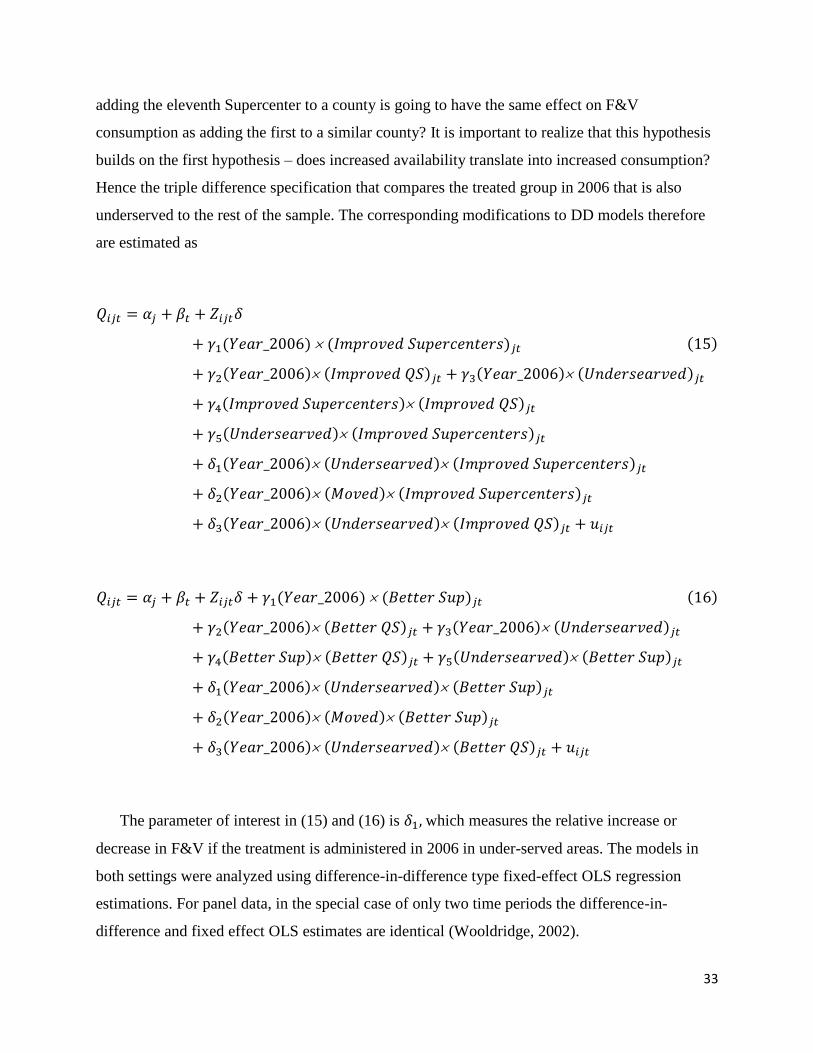
33

adding the eleventh Supercenter to a county is going to have the same effect on F&V

consumption as adding the first to a similar county? It is important to realize that this hypothesis

builds on the first hypothesis – does increased availability translate into increased consumption?

Hence the triple difference specification that compares the treated group in 2006 that is also

underserved to the rest of the sample. The corresponding modifications to DD models therefore

are estimated as

( ) ( ) ( )

( ) ( ) ( ) ( )

( ) ( )

( ) ( )

( ) ( ) ( )

( ) ( ) ( )

( ) ( ) ( )

( ) ( ) ( )

( ) ( ) ( ) ( )

( ) ( ) ( ) ( )

( ) ( ) ( )

( ) ( ) ( )

( ) ( ) ( )

The parameter of interest in (15) and (16) is which measures the relative increase or

decrease in F&V if the treatment is administered in 2006 in under-served areas. The models in

both settings were analyzed using difference-in-difference type fixed-effect OLS regression

estimations. For panel data, in the special case of only two time periods the difference-in-

difference and fixed effect OLS estimates are identical (Wooldridge, 2002).

34

Data and Summary Statistics

We draw on 2005 and 2006 County Business Patterns and Population Estimates, U.S. Census

Bureau, to delineate the food retail environment and the population/area estimates for the

geographical units in our analysis. We then align the information on food access with actual

household purchase data from the Nielsen panel from the same areas or counties for the same

period.

Although the Nielsen HomeScan data are collected from a nationally representative cross

section of households over time, the data set is referred to as panel as a sizable portion of the

households continue the membership from one year to the next. There were 38,802 and 37,719

households participating in the Nielsen panel for 2005 and 2006, respectively. Altogether there

were 46,301 households that participated in one year or both. A panel of 30,269 households or

approximately 78% and 80% of 2005 and 2006 cross-sections, respectively, participated in both

years.

The food accessibility data, obtained from the County Business Patterns, U.S. Census

Bureau, include the number of establishments of the following store formats: supercenters and

price clubs (hereafter Supercenters, including North American Industry Classification System

(NAICS) codes 44511 and 452910) and quick-service restaurants (hereafter QS, including

NAICS code 7222) for 3,091 counties. For each county a binary variable ‘Improved

Supercenters’ was created that equals to unity if the number of establishments (NAICS codes

44511 and 452910) has increased from 2005 to 2006. A similar variable was created for the

quick-service restaurants – ‘Improved QS’. Many studies on food deserts use commuting

distance of 10 miles or more as an indicator for food deserts. Following these studies, we

identified counties that have 1 or less supercenters per 31411

square miles as ‘Underserved’.

An indicator variable ‘Better Sup’ was created to indicate if the household exposed to better

retail conditions in 2006 due to increase in the number of Supercenters in the residence county

from 2005 to 2006, or due to moving to a new county with a higher number of Supercenters in

2006. A similar variable was created to indicate an increased access to QS restaurants – ‘Better

QS’. In case the households moved, the Supercenters and QS variables were adjusted by

11

An alternative definition of ‘Underserved’ – differentiated by Metropolitan or Micropolitan Areas, with 1and 3

miles or more for metro areas and 10 miles for non-metro areas, was used for the robustness check of the results.

The results were close to the reported ones and, therefore, are not reported in the Results section.

35

expressing the levels by 100 square miles. A binary variable ‘Moved’ was created to capture the

change due to moving to a new place. Quantity and Price measure the quantity in ounces and

price per ounce of fresh and processed F&V.

The descriptive statistics of the full set of variables for the panel are in Table 6. Households

in the panel sample purchase slightly more F&V than households in the cross-sectional sample in

general. In both samples the purchase quantity decreased from 2005 to 2006, while the mean

price increased from $0.100/oz to $0.106/oz. In 2006 approximately 80% of panel sample is in

the highest income groups, with 9% being in the lowest income groups.

Approximately 33% of the sample in both years resided in counties that experienced an

increase in Supercenters in 2006. 33% of households were exposed to increased Supercenters

availability due to either increase in the number of establishments in their respective counties (if

stayed) or due to moving to counties with higher number of establishments. Approximately 15%

of households reside in counties that were under-served in 2005.

The demographic information indicates that approximately 59% of households were married,

with 2.3 members, on average. 37% and 36% of female household heads are full-time employed

in the cross-section and panel samples, respectively. The full-time employment rates for male

household heads are slightly lower in the panel sample than in the cross-sectional sample with

both declining in 2006. The educational attainment for female household heads is consistently

higher than that of male household heads. In 2005 and 2006, 79.3% and 80.6% of households in

the panel sample had no children under 18 in the household.

36

Table 6. Descriptive Statistics of Variables in the Cross-Sectional and Panel Samples.

Variable

Control (20,165 HHDs)

Treatment

(10,104 HHDs)

33.38%

Mean Std Mean Std

F&V Quantity (annual, oz) 1282.500 967.711 1289.250 1003.730

Price (average, oz) 0.287 0.116 0.299 0.132

Poverty Income Ratio (PIR) 3.841 2.461 4.111 2.587

Income

Income 1 (= 1 if PIR < 1.30) 0.078 0.268 0.070 0.256

Income 2 (= 1 if 1.30 ≤ PIR < 1.85) 0.135 0.341 0.115 0.319

Income 3 (= 1 if 1.85 ≤ PIR < 2.50) 0.133 0.340 0.115 0.320

Income 4 (= 1 if 2.50 ≤ PIR < 4.00) 0.266 0.442 0.263 0.440

Income 5 (= 1 if 4.00 ≤ PIR ) 0.388 0.487 0.436 0.496

Treatment

Better Conv (= 1 if in 2006 hhd has access to

increased number of Convenience)

0.172

0.377

0.144

0.351

Better Spec (= 1 if in 2006 hhd has access to

increased number of Specialty)

0.286

0.452

0.443

0.497

Better FS (= 1 if in 2006 hhd has access to

increased number of FS)

0.527

0.499

0.654

0.476

Better QS (= 1 if in 2006 hhd has access to

increased number of QS)

0.591

0.492

0.683

0.465

Underserved (= 1 if county has less than 1

Supercenters per 314 sq. mile)

0.819

0.385

0.724

0.447

Married (= 1 if married) 0.590 0.492 0.581 0.493

Household Size 2.257 1.234 2.251 1.227

Moved 0.031 0.174 0.014 0.116

Female Head Age

No Female Head 0.103 0.304 0.111 0.314

Under 45 Years 0.180 0.384 0.196 0.397

45-54 Years 0.235 0.424 0.245 0.430

55+ Years 0.483 0.500 0.448 0.497

Male Head Age

No Male Head 0.276 0.447 0.277 0.448

Under 45 Years 0.140 0.347 0.156 0.363

45-54 Years 0.192 0.394 0.196 0.397

55+ Years 0.392 0.488 0.371 0.483

37

Table 6. – Continued.

Variable

Control (20,165 HHDs)

Treatment

(10,104 HHDs)

33.38%

Mean Std Mean Std

At least one child under 18 0.020 0.141 0.025 0.155

Female Head Employment

Part time 0.144 0.351 0.142 0.349

Full time 0.356 0.479 0.366 0.482

Male Head Employment

Part time 0.051 0.219 0.051 0.220

Full time 0.415 0.493 0.433 0.496

Female Head Education

High school or less 0.300 0.458 0.273 0.446

Some college or more 0.597 0.490 0.616 0.486

Male Head Education

High school or less 0.242 0.429 0.219 0.414

Some college or more 0.482 0.500 0.504 0.500

Hispanic 1.938 0.241 1.951 0.216

Race non-white 0.148 0.355 0.182 0.386

Results

Table 7 shows the OLS estimates from the panel analysis. The results for DD and DDD

specifications are presented for the pooled sample (columns 1 and 2) and for subsamples by

income group (columns 3 to 8). The dependent variable is the natural logarithm of the number of

ounces of F&V purchased. All standard errors are corrected for heteroskedasticity, but not for

intragroup correlation (Donald and Lang, 2007; Moulton, 1990; Moulton, 1986; Conley and

Taber, 2011).

In general, the results do not support either hypothesis this research addresses. The results

demonstrate that there is no indication that food availability has any causal effect on the food

choice.

38

Table 2. Impact of Improved Grocery Access on Household Fruit and Vegetable Purchases – Difference-in-Difference and

Triple Difference Analysis of Panel Data.

Full Sample Income 1

PIR < 1.30

Income 2

1.30 ≤ PIR < 1.85

Income 3

1.85 ≤ PIR < 2.50

Income 4

2.50 ≤ PIR < 4.00

Income 5

4.00 ≤ PIR

DD

(1)

DDD

(2)

DD

(3)

DDD

(4)

DD

(5)

DDD

(6)

DD

(7)

DDD

(8)

DD

(9)

DDD

(10)

DD

(11)

DDD

(12)

(Year_2006)

(Better Supercenters)

-0.032

(0.022)

-0.048

(0.045)

-0.043

(0.102)

0.022

(0.070)

-0.010

(0.059)

0.021

(0.054)

-0.021

(0.062)

0.033

(0.168)

-0.040

(0.041)

-0.096

(0.086)

-0.031

(0.032)

-0.043

(0.067)

(Year_2006)

(Better Convenience)

-0.028

(0.025)

-0.028

(0.025)

-0.091

(0.090)

-0.090

(0.053)

-0.002

(0.079)

-0.003

(0.042)

-0.118

(0.071)

-0.118

(0.071)

-0.048

(0.048)

-0.046

(0.048)

0.007

(0.037)

0.007

(0.037)

(Year_2006)

(Better Specialty)

0.019

(0.021)

0.019

(0.021)

-0.079

(0.077)

-0.080

(0.045)

0.007

(0.060)

0.006

(0.034)

0.040

(0.066)

0.036

(0.066)

0.089*

(0.040)

0.091*

(0.040)

0.004

(0.030)

0.004

(0.030)

(Year_2006)

(Better FS)

0.004

(0.019)

0.004

(0.019)

0.013

(0.077)

0.012

(0.042)

0.004

(0.049)

0.004

(0.031)

0.021

(0.061)

0.017

(0.060)

0.021

(0.037)

0.022

(0.037)

-0.021

(0.029)

-0.022

(0.029)

(Year_2006)

(Better QS)

0.022

(0.020)

0.013

(0.044)

0.100

(0.075)

0.046

(0.067)

0.053

(0.050)

0.078

(0.051)

-0.032

(0.064)

-0.106

(0.167)

-0.002

(0.038)

-0.014

(0.081)

0.019

(0.031)

0.010

(0.068)

(Year_2006)

(Underserved)

(Better Supercenters)

0.020

(0.051)

-0.086

(0.092)

-0.041

(0.068)

-0.072

(0.177)

0.074

(0.096)

0.016

(0.075)

(Year_2006)

(Underserved)

(Better QS)

0.010

(0.024)

0.071

(0.084)

-0.031

(0.063)

0.095

(0.176)

0.013

(0.091)

0.010

(0.076)

(Year_2006)

(Better Supercenters)

(Moved)

-0.022

(0.044)

0.076

(0.152)

-0.020

(0.107)

-0.087

(0.103)

0.108

(0.088)

-0.040

(0.077)

F-Value 5.05

(<.0001)

5.04

(<.0001)

2.43

(<.0001)

2.42

(<.0001)

2.09

(<.0001)

2.08

(<.0001)

1.92

(<.0001)

1.92

(<.0001)

2.85

(<.0001)

2.85

(<.0001)

3.13

(<.0001)

3.12

(<.0001)

R-Square 0.1717 0.1727 0.4459 0.4459 0.3259 0.3259 0.3150 0.3151 0.2543 0.2544 0.1880 0.1881

Adj R-Sq 0.1385 0.1384 0.2625 0.2619 0.1696 0.1693 0.1511 0.1508 0.1651 0.1651 0.1279 0.1278

Sample Size 60,528 60,528 4,561 4,561 7,753 7,753 7,697 7,697 16,037 16,037 24,480 24,480

39

The parameter estimates of interest in the panel models, namely the parameter estimates to

variables that indicate (i) the households that have better access in 2006 than in 2005 purchase

more, and (ii) the households that are from underserved areas and have better access in 2006 than

in 2005 purchase more, are presented in Table 3. The results indicate that none of and are

significant in any of the models (Table 7).

Based on the estimation results from the pooled sample and Income 1 group subsample,

households that were exposed to better retail environment due to moving purchase significantly

more (2.29oz) compared to the control group. So did households from counties that experienced

increase in Supercenters and QS outlets (pooled sample and Income 1 subsample only). In the

pooled model households that resided in under-served areas and that faced increased QS

availability purchased significantly less F&V ( ).

Concluding Remarks

The literature findings on the linkage of diets with metabolic diseases motivated a host of

empirical studies seeking to shed light on the reasons giving rise to particular food choices or

patterns of it. A favorite factor considered by the professional community and public press is the

neighborhood food environment or food availability. Despite the logical appeal, there does not

seem to be conclusive evidence in the literature on the existence or the nature of such linkage.

This research aims to shed light on some aspects of this question. In particular we seek to answer

two questions: (1) is there a positive relationship between the number of stores available in each

location and F&V consumption by the households in that location? and (2) is there a pronounced

relationship in low-income, under-served neighborhoods?

We use national level purchase data for two years – 2005 and 2006, in a difference-in-

difference type fixed effects OLS estimation to model the relationship between food availability

and food choice. The analyses were replicated for cross-sectional and panel samples from these

two years. Our results suggest no statistically significant association between food access and

food choice. No statistical significance emerged when estimating the same models for

subsamples determined by different income levels. Based on the current results, the conclusion

we offer is that the objective of improving the population’s diet through increasing F&V

consumption may be attained through increasing food retail outlet availability.

40

The shortcomings of this research may motivate the need for the future research that will

help with a more comprehensive analysis. The current research disregards the bordering effects –

it views counties separately, not in the context of clusters. The replication of the current analysis

with Metropolitan Statistical Areas as the unit of residence may help with confirming the

robustness of our findings. Given the separate findings in the literature, it also may prove helpful

to conduct this analysis separately for fruits and vegetable, and separately for fresh and non-fresh

produce.

Another shortcoming that could possibly confound the true effects is disregarding the

magnitude or the length of the treatment – we account for an increase, but not the size of the

increase, or the time span of the exposition to the supply shock. Our indication variable for the

increase does not account for how many more stores were added to the neighborhood, or how big

the new stores are. The current data do not allow for estimating the improvement of the current

stores as well, which may be useful information to account.

41

VI. The Effect of Food Store Access and Income on Household Food Purchases: An AIDS

Demand Analysis

This Section builds on Section IV above by extending the analysis beyond F&Vs. Our aim is to

build a demand model for major food groups mentioned in the Dietary Guidelines for a balanced

mixture of healthy and unhealthy foods. The food groups considered for this analysis are fruits,

vegetables, whole grains, milk, meats (not including fish and shellfish), eggs, oils and fats,

carbonated soft drinks and other sugary drinks, snacks and alcohol. The focus on a basket of

foods rather than any particular food is noteworthy for explaining the maximum impact of supply

shocks on diet in general.

Model

The Almost Ideal Demand System (AIDS) can be expressed as follows:

∑

(

) ( )

where is the budget share of the ith

food, , is the price of kth

food, is the

expenditure on all foods, ( ) ∑ ∑

.

The store density variables are appended to (1) through a linear translation

∑

( )

where is the number of retail outlets of type , .

The restrictions for additivity, symmetry and homogeneity were imposed. The Stone price index

was constructed as a linear approximation of the AIDS price index. Finally, block separability

was assumed to estimate the demand system (1).

42

Data and Summary Statistics

We draw on 2006 County Business Patterns and Population Estimates, U.S. Census Bureau, to

delineate the food retail environment and the population/area estimates for the geographical units

in our analysis. We then align the information on food access with actual household purchase

data from the Nielsen panel from the same areas or counties for the same period. Purchase prices

and expenditures on 10 food groups for 37,520 households in the Nielsen panel for 2006 were

used for the analysis. The shares of expenditure on each food group for the pooled sample and

subsamples by income groups are presented in Table 1. The households in the high income

subsample (PIR > 4.00) spend a larger proportion of their expenditures on fruit, vegetables,

whole grains and alcohol. The subsample in the lowest income group (PIR<1.30) spends larger

proportion of their expenditures on all other food groups the subsample. Similarly the

Table 8. Shares of Food Expenditures and Food Access by Income Group.

Food Group

Full Sample Income 1

PIR < 1.30

Income 2

1.30≤PIR<1.85

Income 3

1.85≤PIR<2.50

Income 4

2.50≤PIR<4.00

Income 5

4.00 ≤ PIR

Mean Food Expenditure Shares

Fruits 0.101 0.087 0.100 0.097 0.098 0.107

Vegetables 0.090 0.085 0.090 0.091 0.090 0.091

Whole Grains 0.031 0.026 0.031 0.030 0.031 0.032

Milk 0.070 0.080 0.078 0.076 0.071 0.064

Meats 0.128 0.140 0.129 0.132 0.130 0.123

Eggs 0.015 0.017 0.017 0.016 0.015 0.014

Oils 0.040 0.042 0.044 0.042 0.040 0.038

Sugary Drinks 0.119 0.137 0.121 0.120 0.120 0.115

Snacks 0.319 0.332 0.329 0.324 0.325 0.309

Alcohol 0.086 0.056 0.060 0.072 0.079 0.108

Retail Food Density

Supermarket 20.48 16.87 16.01 17.15 19.96 23.93

Convenience 2.47 2.12 1.98 2.18 2.38 2.82

Specialty 5.72 4.56 4.47 4.75 5.52 6.77

Full Service 125.07 99.23 99.19 107.17 121.97 145.53

Quick Service 210.58 168.09 167.39 182.40 204.51 244.58

43

subsample in the highest income group has more access to all kinds of retail food outlets

compared to the lowest income group.

Results

Table 9 shows the estimates from the AIDS analysis. The results indicate that there is a mild

increase in the elasticity of demand for fruits and whole grains per 1% increase in supermarkets

for the pooled sample. The results for subsamples by income group indicate that the effect is

entirely due to the positive significant elasticity apparent in the highest income group. The

demand for meat in the pooled sample and income subsamples demonstrate positive significant

elasticities of supermarket density. This indicates that a 1% increase in supermarkets in the

county induces positive proportional increase in the meat demand for households regardless of

income groups. A 1% increase in supermarket availability for the households in the lowest

Table 9. Supermarket Elasticities of Food Groups by Income Groups and for the Pooled

Sample.

Food Group

Full Sample Income 1

PIR < 1.30

Income 2

1.30≤PIR<1.85

Income 3

1.85≤PIR<2.50

Income 4

2.50≤PIR<4.00

Income 5

4.00 ≤ PIR

Fruits

0.0135*

(0.0058)

-0.0194

(0.0222)

-0.0018

(0.0153)

-0.0062

(0.0144)

0.0037

(0.0115)

0.0329**

(0.0096)

Vegetables

0.0075

(0.0046)

-0.0166

(0.0166)

0.0045

(0.0121)

0.0150

(0.0115)

0.0138

(0.0090)

0.0102

(0.0075)

Whole Grains

0.0235**

(0.0086)

-0.0052

(0.0335)

0.0220

(0.0236)

0.0189

(0.0210)

0.0337*

(0.0169)

0.0237

(0.0138)

Milk

-0.0046

(0.0063)

0.0074

(0.0208)

0.0282

(0.0160)

-0.0280

(0.0146)

-0.0084

(0.0121)

0.0049

(0.0108)

Meats

0.0479**

(0.0054)

0.0669**

(0.0175)

0.0418**

(0.0135)

0.0382**

(0.0123)

0.0576**

(0.0104)

0.0558**

(0.0094)

Eggs

0.0083

(0.0072)

0.0007

(0.0283)

0.0466*

(0.0183)

-0.0106

(0.0160)

0.0392**

(0.0140)

-0.0043

(0.0122)

Oils

0.0110

(0.0057)

-0.0192

(0.0214)

-0.0077

(0.0157)

0.0305*

(0.0137)

0.0230*

(0.0108)

0.0167

(0.0095)

Sugary Drinks

0.0018

(0.0061)

0.0474*

(0.0205)

0.0179

(0.0166)

-0.0116

(0.0147)

-0.0154

(0.0119)

0.0008

(0.0101)

Snacks

-0.0058

(0.0031)

-0.0329**

(0.0103)

-0.0181*

(0.0081)

0.0021

(0.0073)

0.0038

(0.0059)

-0.0088

(0.0054)

Alcohol

-0.0869**

(0.0127)

-0.0264

(0.0541)

-0.0865*

(0.0415)

-0.0649

(0.0345)

-0.1313**

(0.0266)

-0.0952**

(0.0188)

Sample Size 37,520 2,825 4,613 5,272 9,376 15,433

44

income group increase and decrease their demand for carbonated sweet drinks and snacks,

respectively. The highly significant negative elasticity of the demand for alcohol in the pooled

sample is largely driven by that of the demand of the highest income groups. The demand for

vegetables and milk seems to be non-responsive to changes in supermarket availability.

Concluding Remarks

Our results suggest that the demand for fruits and whole grains responds positively to changes in

the supermarket availability only in the high income subsample, leaving the poor largely non-

responsive to the changes in the retail environment. The demand for vegetables and milk is

invariant to changes in the supermarket availability regardless of income level. The demand for

carbonated soft drinks in the lowest income group increases with the increased supermarket

availability. The effects on the demand for snacks are negative indicating that the households in

the lowest income group would actually decrease their demand for snacks as a response to a 1%

increase in the supermarket availability.

From these results it would appear that an increase in the supermarket availability would

induce increased healthy food (fruits and whole grains) and decrease ‘unhealthy’ food (alcohol)

demands in the high income groups. In the low income groups, a 1% increase in the supermarket

availability appears to have no effect on any healthy food demand, hand have ambiguous effects

on unhealthy food (carbonated soft drinks and other sugary fruit drinks, and sweet and non-sweet

snacks) demand. These suggest that increased availability will possibly have ambiguous effects

on diet, especially that of the population in the low income groups.

45

VII. Conclusion

Limited access to healthy food has been linked to poor diets and adverse health effects

particularly in underserved and predominantly poor communities. The objective of this research

is to identify the influence of food access factors on healthy food purchases using retail food

availability data, detailed purchase scanner data. We demonstrate that the densities of

supermarkets in Metropolitan Statistical Areas or counties induce significant positive effects in

‘healthy’ food demand in the high income groups. The effect on the ‘healthy’ food purchases by

low income population is insignificant. On the other hand, the effects of increased availability on

‘unhealthy’ food consumption are ambiguous for the low income population.

The current findings of this project suggest that the objective of improving diet may be

unattainable by solely increasing supermarket or other large retailer availability, especially for

the low income population. To conclusively answer this question more research is needed that

would account for the length and magnitude of increased availability.

46

References

Beaulac, J., E. Kristjansson, and S. Cummins. 2009. A Systematic Review of Food Deserts,

1966-2007. Preventing Chronic Disease 6(3):A105-A115.

Bitler, M., and S.J. Haider. 2011. An Economic View of Food Deserts in the United States.

Journal of Policy Analysis and Management 30(1):153-176.

Blanchard, T.C., and T.A. Lyson. 2002. Retail Concentration, Food Deserts, and Food

Disadvantaged Communities in Rural America. Article ed. Mississippi State University.

Bodor, J.N., D. Rose, T.A. Farley, C. Swalm, and S.K. Scott. 2007. Neighborhood Fruit and

Vegetable Availability and Consumption: the Role of Small Food Stores in an Urban

Environment. Public Health Nutrition 11(4):413-420.

Broda, C., E. Leibtag, and D.E. Weinstein. 2009. The Role of Prices in Measuring the Poor’s

Living Standards. Journal of Economic Perspectives 23(2): 77-97.

Chintagunta, P.K., D.C. Jain, and N.J. Vilcassim. 1991. Investigation Heterogeneity in Brand

Preferences in Logit Models for Panel Data. Journal of Marketing Research 28: 417-428.

Conley, T.G., and C.R.Taber. 2011. Inference with “Difference in Differences” with Small

Number of Policy Changes. The Review of Economics and Statistics 93(1): 113-125.

Courtemanche, C., and A. Carden. 2011. Supersizing Supercenters? The Impact of Walmart

Supercenters on Body Mass Index and Obesity. Journal of Urban Economics 69: 165-181.

Cummins, S., M. Petticrew, C. Higgins, A. Findlay, and L. Sparks. 2005. Large Scale Food

Retailing as an Intervention for Diet and Health: Quasi-Experimental Evaluation of a Natural

Experiment. Journal of Epidemiology and Community Health 59: 1035-1040.

Donald, S.G., and K. Lang. 2007. Inference with Difference-in-Difference and Other Panel Data.

The Review of Economics and Statistics 89(2): 221-233.

Dong, D., and H. Stewart. 2012. Modeling a Household’s Choice among Food Store Types.

American Journal of Agricultural Economics 94(3): 702-717.

Fader, P.S., and J.M. Lattin. 1993. Accounting for Heterogeneity and Nonstationarity in a Cross-

Sectional Model of Consumer Purchase Behavior. Marketing Science 12(3): 304-317.

Fader, P.S., J.M. Lattin, and J.D.C. Little. 1992. Estimating Nonlinear Parameters in the

Multinomial Logit Model. Marketing Science 11(4): 372-385.

Guadagni, M.P., and J.D.C. little. 1983. A Logit Model of Brand Choice Calibrated on Scanner

Data. Marketing Science 2(3): 203-238.

Hausman, J., and E. Leibtag. 2004. CPI Bias from Supercenters: Does the BLS Know That Wal-

Mart Exists?” NBER Working Paper 10712.

Hausman, J., and E. Leibtag. 2007. Consumer Benefits from Increased Competition in Shopping

Outlets: Measuring the Effect of Wal-Mart. Journal of Applied Econometrics 22: 1157-1177.

47

Hellerstein, J., D. Neumark, and M. McIrerney. 2008. Spatial Mismatch or Racial Mismatch?

Journal of Urban Economics 64: 464-479.

Holmes, T.J. 2011. The Diffusion of Wal-Mart and Economies of Density. Econometrica 79(1):

253-302.

Kyureghian, G., O. Capps Jr., and R. M. Nayga, Jr. 2011. A Missing Variable Imputation

Methodology with an Empirical Application. Advances in Econometrics 27: 313-337.

Kyureghian, G., and R.M. Nayga Jr. 2012(a). The Role of Food Access in Meeting Some

Dietary Guidelines: A Natural Experiment. Selected Paper for 2012 Agricultural & Applied

Economics Association Annual Meeting.

Kyureghian, G, and R.M. Nayga Jr. 2012(b). Food Store Access, Availability and Choice When

Purchasing Fruits and Vegetables. American Journal of Agricultural Economics. Forthcoming.

Kyureghian, G., R.M. Nayga, Jr., and S. Bhattacharya. 2012. The Effect of Food Store Access

and Income on Household Purchases of Fruits and Vegetables: A Mixed Effect Analysis at the

County and MSA levels. Agricultural Economic Perspectives ad Policy. Forthcoming.

Laraia, B.A., A.M. Siega-Riz, C. Gundersen, and N. Dole. 2006. Psychosocial Factors and

Socioeconomic Indicators Are Associated with Household Food Insecurity among Pregnant

Women. The Journal of Nutrition 136: 177-182.

Larsen, K., and J. Gilliland. 2009. A Farmers’ Market in a Food Desert: Evaluating Impacts on

the Price and Availability of Healthy Food. Health & Place 15: 1158-1162.

Larson, N.I., M.T. Story, and M.C. Nelson. 2009. Neighborhood Environments: Disparities in

Access to Healthy Foods in the U.S. American Journal of Preventative Medicine 36(1):74-

81.e10.

Liese A., Battersby S., and Bell B. 2012. Identifying Food Deserts in the Rural South: A

Comparison of Food Access Measures. Food Assistance Programs, Food Access and Choices,

and Obesity and Other Health Outcomes. Research Innovation and Development Grants in

Economics (RIDGE) Conference, Washington, DC, October 2012.

Littell, R.C., G.A. Milliken, W.W. Stroup, R.D. Wolfinger, and O. Schabenberger. 2006. SAS

for Mixed Models. Second Edition. Cary, NC, SAS Institute Inc.

McFadden, D. 1973. Conditional Logit Analysis of Qualitative Choice Behavior. in Frontiers in

Econometrics, ed. by P. Zarembka. New York: Academic Press, 105-142.

Michimi, A., and M.C. Wimberly. 2010. Associations of Supermarket Accessibility with Obesity

and Fruit and Vegetable Consumption in Conterminous United States. International Journal of

Health Geographics 9(49):1-14.

Moulton, B.R. 1990. An Illustration of a Pitfall in Estimating the Effect of Aggregate Variables

on Micro Units. The Review of Economics and Statistics 72: 334-338.

Moulton, B.R. 1986. Random Group Effects and the Precision of Regression Estimates. Journal

of Econometrics 32: 385-397.

48

Neckerman, K. M. Bader, M. Purciel, and P. Yousefzadeh. 2009. Measuring Food Access in

urban areas. Accessed at: http://www.npc.umich.edu/news/events/food-access/index.php.

Nevo, A. 2001. Measuring Market Power in the Ready-to-Eat Cereal Industry. Econometrica 69

(2): 307-342.

Pearson, T., J. Russell, M.J. Campbell, and M.E. Barker. 2005. Do ‘Food Deserts’ Influence

Fruit and Vegetable Consumption? – A Cross-Sectional Study. Appetite 45:195-197.

Rose, D. M., J.N. Border, C. M. Swalm, J.C. Rice, T.A. Farley, and P.L. Hutchinson. 2009.

Deserts in Orleans? Illustrations of Urban Food Access and Implications for Policy. Accessed at:

http:// www.npc.umich.edu/news/events/food-access/index.php.

Rose, D., and R. Richards. 2004. Food Store Access and Household Use among Participants in

the US Food Stamp Program. Public Health Nutrition 7(8):1081-1088.

Searle, S. R., Casella, G., and McCulloch, C. E. 1992. Variance Components, New York: John

Wiley & Sons.

Sharkey, J.R., and S. Horel. 2009. Characteristics of Potential Spatial Access to a Variety of

Fruits and Vegetables in a Large Rural area. Accessed at: http://

www.npc.umich.edu/news/events/food-access/index.php.

Sharkey, J.R., S. Horel, W.R. Dean. 2010. Neighborhood Deprivation, Vehicle Ownership, and

Potential Spatial Access to a Variety of Fruits and Vegetables in a Large Rural Area in Texas.

International Journal of Health Geographics 9:26.

Staus, A. 2009. Determinants of Store Type Choice in the Food Market for Fruits and

Vegetables. International Journal of Arts and Sciences 3(2): 138-174.

United States Department of Agriculture. 2009. Access to Affordable and Nutritious Food:

Measuring and Understanding Food Deserts and Their Consequences. Report to Congress.

Accessed at: http://www.ers.usda.gov/publications/AboutPDF.

Wooldridge, J. M. 2002. Econometric Analysis of Cross Section and Panel Data. Massachusetts

Institute of Technology Press.

Xu, L. and J. Shao. 2009. Estimation in Longitudinal or Panel Data Models with Random-Effect-

Based Missing Responses, Biometrics 65, 1175-1183.