Follow the Money: Models of Congressional Governance and the Appropriations Process

John H. Aldrich, Duke University Brad T. Gomez, Florida State University

Jennifer L. Merolla, Claremont Graduate University

John H. Aldrich is Pfizer-Pratt University Professor of Political Science, Duke University, 326 Perkins Library, Box 90204, Durham, NC 27708-0204. (aldrich@duke.edu). Brad T. Gomez is Assistant Professor of Political Science, Florida State University, Tallahassee, FL 32306. (bgomez@fsu.edu). Jennifer L. Merolla is Assistant Professor of Politics and Policy, Claremont Graduate University, 160 East Tenth Street, Claremont, CA 91711-6163. (jennifer.merolla@cgu.edu) The authors would like to thank Jim Granato, George Krause, Frances Lee, Michael Munger, and seminar participants at the University of South Carolina, University of North Carolina, and Ohio State University and the reviewers at APSR for their helpful comments. We especially would like to thank Peter Pedroni for supplying and providing assistance with his RATS code for group-mean panel FMOLS. We also are indebted to Annabel Azim, who provided vital research assistance during the early stages of this project.

Follow the Money: Models of Congressional Governance and the Appropriations Process

Abstract

This paper tests competing models of congressional governance as explanations for House

appropriations recommendations. We seek to adjudicate between the committee-dominance model of

Shepsle and Weingast, the floor-dominance model of Krehbiel, the party cartel theory of Cox and

McCubbins, and Aldrich and Rohde’s conditional party government thesis, thus providing the first

simultaneous test of these models as explanations for legislative output. Using appropriations data from

1951 to 1998, we find that the conditional party government thesis easily offers the best explanation for

appropriations behavior. Indeed, during the period under investigation, we find that an empowered

Democratic House leadership was responsible for nearly $1.3 trillion dollars in additional spending.

Introduction

One of the most dramatic changes in American national politics over the last fifty years has been

the increasing polarization of partisan politics, especially in Congress. The typical Democrat in both the

U.S. House and Senate votes considerably more liberally than the average Republican, and this is a

dramatic increase from a generation ago (see Aldrich and Rohde, 2000c; Sinclair, 2000, inter alia).

Accompanying this surge in partisan floor voting is a resurgence of partisan voting in the electorate (e.g.,

Bartels, 2000; Jacobson, 2000). In between the more partisan voter and the more partisan legislator stand

party leadership positions and other institutions of the party-in-government. How consequential these

factors are in the partisan polarization of Washington politics is contentious. Is the increasingly partisan

rhetoric and floor voting due to the increasingly polarized preferences of the legislators that the public has

elected, are they due to the increasingly strong powers of party leaders and institutions within the

chambers, or are they due to both? This debate, in turn, fits smoothly into the more general debate about

the role that all the various institutions of the House (and, sometimes, in the Senate) play in structuring

outcomes. This more general debate is equally as contentious, at least partially based on the same

question – do intra-chamber or at least intra-governmental rules and institutions “matter,” or are outcomes

driven by forces outside of Washington, especially those emanating from the consequences of ex ante and

ex post elections?

This debate has flourished particularly strongly within the rational choice based “new

institutionalism” (see Shepsle and Weingast, 1995, for one review). Typical hypotheses, often rigorously

derived, argue that committees composed of high demanders shape policy, that the floor median

dominates selection of policy outcomes, or that the majority party’s preferences are consequential.1 Note

that these various models differ on an important consequence, the nature of policy adopted in the nation.

Testing these hypotheses, however, has proven difficult, especially on this central question of policy

choices. It is true for all scholars, and not just new institutionalists, that it is very difficult to measure

1 We ignore, for purposes of exposition only, consideration of the necessity to form extraordinary majorities and their associated “pivot points” to override vetoes or, in the Senate, to invoke cloture.

whether one bill is more moderate than some other proposal, or if the legislation just adopted is closer to

the center of the whole chamber or the center of the majority party.

In this paper, we propose a test among four of the major classes of models of congressional policy

making developed by the new institutionalists. To do so, we offer a resolution to several of the major

problems that arise in seeking to test hypotheses about the location of policy outcomes. Central to this

resolution is examining appropriations over a fifty-year interval. First, appropriations provide a

reasonably fixed “metric” of (constant) dollars with jurisdictions of the subcommittees that compose the

Appropriations Committee that have been relatively constant over our time frame. Each subcommittee

reports a bill (or set of bills that can be aggregated to that equivalent) that indicates how much money is

authorized for more or less the same set of possible activities, those that fall within the jurisdiction of the

subcommittee. Thus, we have a measurable outcome that can be compared over time, forming a

reasonably long and wide pooled cross-sectional, time series panel of data. Second, we do not attempt to

map spatial locations, such as the location of the ideal appropriation of the medianth member of the

House, directly onto appropriations. Instead, we look at variation in spatial locations and other

independent variables over time, and see how those variations align with changes in appropriations.

Thus, we can ask questions such as, “When parties are stronger, are changes in the location of the center

of the majority party more closely associated with changes in appropriations than when parties are

weaker?” This question is answerable because the time period we use coincides with considerable

variation in virtually all of the explanatory variables. As implied above, party affiliates are considerably

more polarized today than thirty years ago, providing variation in a number of variables at the core of

party theories. While the location of the center of the floor moves less dramatically than that of the center

of the majority party, the “pivot points” that are critical to the recent versions of floor-centered accounts

(e.g., Krehbiel, 1998; Brady and Volden, 1998) do vary considerably. Most especially, the location of the

relevant veto override point varies dramatically when the president changes from a liberal or moderately

liberal Democrat to a conservative or moderately conservative Republican. Finally, Shepsle, one of the

2

central architects of the committee-centered view, has argued (1989) that the importance of the committee

has altered substantially between the 1960s and 1980s, as the “textbook” view of Congress changed.

In short, just like the admonition from “Deep Throat” to Woodward and Bernstein during

Watergate, we believe that we should “follow the money.” By following the trail of federal

appropriations over time, we will examine a phenomenon of great policy consequence. And we also

believe that, by following the money, we can test such hypotheses as whether money follows the

preferences of majority party in the House, the whole House, or the Appropriations committee.

Appropriations and Theories of Legislative Organization

One benefit to using congressional appropriations is that we are testing hypotheses about matters

that are at the very heart of public policy in America. Not surprisingly, many scholars have studied

congressional spending. The study of budgeting in Congress itself has been dominated for decades by the

work of Wildavsky (1964) and Lindblom (e.g., Dahl and Lindblom, 1976 [1953]), their accounts of

incrementalism, and the extensive testing of specific versions of such views by Davis, Dempster, and

Wildavsky (1966; 1974). Similarly, Fenno’s (1966; 1973) early work represents a benchmark study of

the politics of the Appropriations Committee. Fenno’s study described the appropriations process as one

dominated by stable rules and roles. Within this process, Fenno and Wildavsky argued that the president

acted as an advocate in the process, presenting increases in the budget requests for agencies, while the

House acted as a guardian of the purse by cutting these requests. Fenno (1973) argued that this role of the

House was a result of the norms of minimal partisanship, hard work, and apprenticeship that were

practiced in the Appropriations Committee. Finally, the Senate was characterized as fulfilling the role of

an “appeals court,” of sort, restoring some of the cuts imposed by the House Appropriations Committee.

Fenno (1966) and Davis, Dempster and Wildavsky (1966, 1974) empirically demonstrated support for

these roles using data on appropriations from fiscal year 1947 to 1962, and from fiscal year 1964 to 1968,

respectively.

3

The second generation of scholars focusing on the appropriations process questioned the stability

of the roles first articulated by Fenno and Wildavsky. In particular, many argued that the roles were

reversed in the 1970’s, with the president now acting as a guardian, the House as an advocate, and the

Senate as a negative rather than positive appeals court (Schick 1980; Ippolito 1981; LeLoup 1986;

Wildavsky 1988). Many attributed these changes to institutional reforms in the 1970’s, most notably the

Congressional Budget and Impoundment Control Act of 1974, changes in the rules of selecting committee

chairs (Schick, 1980), and changes in the process of assigning members to committees (LeLoup, 1980).

Some demurred from the conclusion that there was a radical break with the past (Maas 1982; Lowery,

Bookheimer and Malachowski, 1985; Geiger 1994). Geiger, for example, examined recommendations by

the House Appropriations Committee from fiscal year 1963 to 1982 and concluded that, while the House

became less of a guardian after the 1974 reforms, it still acted more like a guardian than an advocate.

Other scholars have assessed how the roles are conditional on the partisan makeup and unification

or division of Congress and the presidency. Lowery, Bookheimer, and Malachowski (1985) reanalyzed

Fenno’s original data and generally supported his conclusions about roles and norms. They also found,

however, that Democratic presidents stimulated the House to impose greater cuts on OMB [BOB]

proposals in the House, while achieving a more successful appeals record in the Senate. Cox, Hager, and

Lowery (1991) extended Fenno’s data to FY 1989 and found that split partisan control of institutions

leads to changes in the committee roles, while unified control lead to the roles first described by Fenno.

Other scholars have examined the impact of the majority party on appropriations, and have found that

party control is stronger under unified control compared to divided control (Kiewiet and McCubbins

1991; Gill and Thurber 1999). Lastly, Aldrich and Rohde (2000b) assessed changes in how the party

leadership sought to use the Appropriations Committee in light of the coming of the Republican majority

in 1995, arguing that the new GOP leadership made especially heavy and partisan use of the committee to

achieve its policy goals. Clearly, the appropriations process is a compelling and multifaceted forum by

which to test alternative theories of congressional governance.

4

Competing Models

In what Fiorina (1987) and Shepsle and Weingast (1995) referred to as the “second generation” of

rational choice models of legislatures, the central objects of study were the committee system with its

procedural rules, system of jurisdictions, and so on (the path breaking model being Shepsle, 1979). This

“generation” of models was concerned with policy outcomes to be sure, but typically focused only on a

particular subset of all possible kinds of legislation, pork barrel or, more generally, distributive outcomes.

This modeling enterprise seemed entirely consistent with a House as described by Mayhew (1974), a

chamber filled with single-minded seekers of reelection who had structured the internal workings of the

House to fit maximally with their reelection needs. This explanation was developed most generally in

Weingast and Marshall (1988), arguing that committees with fixed jurisdictions made possible solution to

a collective action problem. Reelection minded members would value some dimensions of distributive

policies more than others. Typically, a minority would benefit greatly from spending more in an area,

while the majority would be weakly opposed by virtue of the higher taxes that would ensue. A majority

could be formed from this coalition of relatively intense minorities, and the committee system was a

mechanism by which this “giant log roll” could be held together with norms such as deference and

reciprocity. We refer to this theory as the “committee-dominance model.”

Krehbiel (1991), building on his work with Gilligan (e.g., 1989; 1990), developed an alternative

account of the House with a committee system. He proposed understanding it as a system of

specialization and division of labor to develop a more efficient system for acquiring and for using

information. In this view, the House empowered committees to specialize in the writing of effective

legislation to achieve goals commonly shared – or, to be specific, to serve as agents so as to better achieve

the outcome desired by the House as a whole, usually summarized as the ideal point of its medianth voter.

In the final analysis, since all regular legislation, as well as most rules and procedures, must win majority

support on the floor of the House, legislative institutions can best be understood as vehicles for helping

the floor majority achieve its outcomes. Later, Krehbiel considered the role of extraordinary majorities,

via the pivot points of veto over rides and cloture (1988). Yet, while this extension enriched his basic

5

account, it did not alter Krehbiel’s basic contention: when it comes to congressional governance, it is the

floor – not the committee nor party – that rules. Accordingly, we label Krehbiel’s account as the “floor-

dominance model.”

At roughly the same time, two sets of scholars were developing another alternative to the Shepsle,

Weingast, et al., committee-dominance models of Congress. Cox and McCubbins (1991) and Kiewiet

and McCubbins (1991) published two complementary accounts that argued for the importance of the

political party in Congress. Actions might not look particularly partisan, because, in equilibrium, parties

will have successfully and carefully assigned their members to certain committees in order to realize the

party’s goals. Through a logic of delegation, a legislative leviathan (to use their two titles) was created in

which the party was central, and consistently so. If both parties created delegations on the most important

committees that represented each party’s policy interests, the full committee delegation would also mirror

the full chamber. The difference with Krehbiel’s view is that it is the majority party that matters most, so

that the median preference within the majority party membership on the committee and in chamber was

what mattered, not the median preference of the full committee and full floor. We refer to this account as

“party cartel” theory.

Rohde (1991) and Aldrich (1995) developed an alternative view of party to that of the “party as

cartel,” advocated by Cox, Kiewiet, and McCubbins. The Aldrich-Rohde argument (see 1997-1998,

1998, 2000a, 2000b, 2000c, see also Aldrich, Berger, and Rohde, 2002) is that the effect of the party on

outcomes is conditional on intra-party heterogeneity and inter-party differentiation. In particular, the

“strength” of a party inside the legislature is endogenous; it is a matter of choice by the relevant actors

involved. When the affiliates of the party collectively perceive and (by a process of overcoming

collective action problems, quite possibly via the Cox-McCubbins solution of “internalizing externalities”

in its leadership) collectively act on the perception that it is more valuable for them to be a stronger rather

than weaker party, then they will enact strategies (adopt rules, empower leadership positions, and so on)

to make them more effective as a party. They further argue that, especially in the House, a cohesive

majority party has the ability to achieve much. The result is that policy will be more to the liking of the

6

majority party in circumstances in which they choose to act cohesively as a “stronger” party. In

particular, as the condition in what they call “conditional party government” is increasingly well satisfied,

the Aldrich-Rohde theory claims that the majority party will strengthen its procedures or will take other

measures to act “strongly.” In those cases, the majority party will win disproportionately more than when

they are less “strong.” That is, the policy outcome will be closer to the majority party median, relative to

the floor median, the greater the condition in conditional party government is satisfied.

Specification of Hypotheses

In this section, we first introduce the central variables and notation used in this paper. Given its

more complex nature, we also must develop the logic for testing the conditional party government model.

We will then be able to specify a series of testable hypotheses, put in terms of major ideal point locations.

Our hypotheses will be of the form, “As the ideal point of the critical actor or actors in a theory varies

over time, appropriations will vary over time in conjunction with that right-hand-side variation.”

Suppose that policy is primarily unidimensional with legislators having Euclidean preferences (a

la Poole-Rosenthal estimations). The key variables for the first three accounts are the location of the ideal

point of the median member of the Appropriations committee, the median member of the floor, the

location of the veto override (or two-thirds majority) ideal point, and the location of the ideal point of the

median member of the majority party. We also consider the ideal point location of the median member of

the majority party on the Appropriations Committee. These can be given notation by letting xmed denote

the ideal point of the median member of the full House, Appmed denote the ideal point of the median

member of the Appropriations Committee, and mmed denote the ideal point of the median member of the

majority party on the floor. The conditional party government hypothesis is conditional and therefore

requires further development. Let d = | xmed - mmed| denote the distance separating the (aggregated)

preference of the majority party from that of the whole chamber. As this distance increases, there appears

to be more to gain for the majority party acting in concert, and indeed, the Aldrich-Rohde claim is that

7

this is precisely the sort of case in which they expect the condition in conditional party government to be

better satisfied.

The appropriations chosen, then, can be denoted as “a” and a can be assumed to be someplace in

the interval between xmed and mmed. So, a can be expressed as a convex combination of the two options:

a = α( mmed) + (1 - α)(xmed).

If α = 1, then the House is consistently choosing the majority party preferred point. If, instead, α = 0,

then the House is consistently choosing the preferred appropriation of the whole chamber (a similar

formulation would apply at the committee level). The former is a very strong version of the Cox,

Kiewiet, McCubbins claim (much stronger than they make), while the latter is the equally strong version

of the Krehbiel claim.

Note, however, when α equals any constant, the effect of party is not conditional on anything

except the differences in preferences of the majority party compared to the whole House. The Aldrich-

Rohde argument is that α varies, and it varies systematically. In particular, they argue that α varies as a

function of the degree to which the condition in conditional party government (“CPG”) varies. In

particular, as CPG increases, then α increases toward 1. Hence, α varies positively with CPG (or, more

simply, set α = g[CPG] where g is any positive constant). We are now in a position to specify our

hypotheses, seeing that we can sharply distinguish among the competing theories (albeit not quite realize

a set of critical tests). We can then consider how to measure these variables, especially the least familiar,

that which we call here “CPG.”

The above theories yield the following four sets of hypotheses:

1. Committee-Dominant Appropriations: If the Shepsle, Weingast, Marshall account applies to

the appropriations process, then the greatest effect on appropriations should come from changes in the

preferences of the committee as a whole (or its subcommittee counterparts), with a significant although

presumably less substantial influence of the whole chamber. Party preferences (on the floor or in

committee) should not be relevant and therefore α should also be approximately zero. That is:

8

Appmed > xmed > 0,

mmed = α = 0.

2. Floor-Dominant Appropriations: If Krehbiel’s informational account is correct, then

appropriations should be dominated by the floor median. Both due to moral hazard in delegation of

expertise to committees and in provision of at least some (policy) inducement to specialize, there may be

some effect of the committee (or subcommittee) preferences. In no case, however, will any of the party

measures be relevant:

xmed > Appmed > 0,

mmed = α = 0.

We do not include “pivot points” in the above but these are included in our tests. None of the other

explanations, however, seems to us to lead to an expectation that pivot points are irrelevant, so this is not

evidently a discriminating variable.

3. Party Cartel: If Cox, Kiewiet, and McCubbins are correct, there will be a constantly

important role for the political party. One might draw an inference from their work that the party in the

committee or subcommittee is to reflect the wishes of the full party in the legislature, and therefore might

have a more modest (even zero) effect on appropriations, but we will not distinguish sharply in either

party theory between the party on the floor and that on the committee. Thus:

xmed = Appmed = 0,

mmed > 0

α = 1.

4. Conditional Party Government: Finally, if the Aldrich and Rohde explanation is correct, we

expect that:

xmed > Appmed ≥ 0,

mmed > 0

α > 0 with α(CPG), such as α = g(CPG), where g is a positive monotonic transformation.

9

Data Description

To test the four sets of hypotheses, we need measures of the ideological composition of the House

as well as measures of the outputs of the policy process. The first stage of our data collection effort was

to obtain measures of appropriations over time. We began with data collected by Kiewiet and

McCubbins’ (1991), which extended from fiscal year 1948 to fiscal year 1985. Their data are broken

down by agency by fiscal year and contains information on the nominal appropriations to each agency

and the bill number from which the Appropriation was taken.2 They also collected the nominal requests

by the president, and in the House and Senate bill, as well as the nominal amount passed by the House

Appropriations Committee, the Senate Appropriations Committee, the House and Senate. We extended

this data to FY 1998 and also collected additional information for the whole time series on the name of

the bill, as well as the committees and subcommittees to which the bills were referred.3 The nominal

appropriations requests were then readjusted according to 1982-1984 fiscal year dollars, to allow for

comparison across years.4

Since our main concern is whether the committee, floor, majority party, or some combination

thereof moves policy closer to their respective median, we need to account for the process of legislating.

Appropriations bills are referred to the subcommittees of the Appropriations Committee, which then

report separate bills that contains appropriations to numerous agencies.5 Since members do not vote on

2 Their data set contains 75 programs and agencies. Thirty-three were also used in Fenno’s study, while the remaining include regulatory agencies, housing programs, and state and defense related programs. 3 We collected data only on those agencies listed in 1985 and extended through 1998. We obtained the data from the Commerce Clearing House (CCH) Congressional Index and CQ Almanac. During the process of adding committee and subcommittee variables to the original Kiewiet and McCubbins data, we found some discrepancies between appropriations records in the CQ Almanac and the dataset. When found, we changed the discrepancies in the dataset to reflect the amount reported in the CQ Almanac. 4 The data used are budget authority, or the amount that the House bill authorized, rather than budget outlays, the amount spent by the given agency or program. 5 Appropriations bills do not follow the same process as regular bills. First, the President submits requests for funds. Often the bill does not appear until the House Appropriations Committee marks up or reports the measure, and often the bill is introduced, referred and reported on the same day (Schick, 1980). The process has changed over our time series, especially with the adoption of the Congressional Budget and Impoundment Control Act of 1974. See below for more information.

10

the amount appropriated to specific agencies, but vote instead on each of the thirteen appropriation bills,

we aggregate the data to reflect the respective subcommittee jurisdictions. Thus, our unit of analysis

becomes “subcommittee appropriation per fiscal year.” For example, the appropriation for the

Subcommittee on Defense is the total appropriations recommended in the House bill to each of the

agencies that were referred to this subcommittee.

There are 11 subcommittees for which we have data, most of which existed in fiscal year 1951.6

The following subcommittees were added to the data set the year in which they appeared in the CCH

Congressional Index or the CQ Almanac: Defense (1961), Foreign Operations (1955), Military

Construction (1960), Transportation (1968), and Public Works (now Energy and Water Development)

(1956). Combining the cross-section, or subcommittee, and the time series, fiscal year, yielded an

unbalanced panel with an overall n of 478.

The second part of our data collection required data on the ideological composition of the House.

For this, we employed Poole and Rosenthal’s NOMINATE scores as a means of determining the floor

median, the majority and minority party medians, as well as the medians of the Appropriations

Committee, its subcommittees and the party entities of each. The NOMINATE scores also were used in

the construction of the Aldrich, Rohde, and Berger (2002) CPG measure described below. These data

were then merged with the appropriations data by fiscal year and subcommittee.

Dependent Variable

There are a variety of dependent measures that could be used: appropriations as recommended by

the committee to the floor, the amount passed by the House initially, the amount passed after any

conferencing with the Senate, the amount signed into law (possibly after vetoes, etc.), or the amount

actually spent in a given fiscal year. The dependent variable we use is the amount of spending authorized

by the House through passage of each of the appropriations bills for each fiscal year, in 82-84 constant

6 Our time series begins in 1951, since data from FY 1950 are incomplete. Also, we do not include appropriations bills from the Subcommittee on the District of Columbia nor the Legislative.

11

dollars.7 We believe this variable to be the best measure of what the House would like to see allocated

that year, recognizing that this amount (compared to the amount that is eventually signed into law) may

be strategically chosen due to anticipated actions by the Senate or president.

Figure 1A show the trend in appropriations by subcommittee from fiscal year 1948 to fiscal year

1998. The most obvious trend is the huge increase in appropriations to the agencies under the jurisdiction

of the Subcommittee on Defense. The figure shows a big increase during the Reagan and Bush I

presidencies, reflecting bipartisan agreement for defense spending since the Democrats were in control of

the House. This substantial increase in spending dissipated quickly under unified government early in the

Clinton administration, only to return with the Republican takeover of the House in 1995. The sheer size

of the budget for the agencies under the jurisdiction of the Subcommittee on Defense masks any

trends that might be occurring in the amount appropriated across the other subcommittees.

[Figure 1A about here]

To get a better picture of the temporal variation in appropriations for other jurisdictions,

we take out the Subcommittee on Defense and split the sample in half from fiscal year 1951 to

1975 and fiscal year 1976 to 1998. Figures 1B and 1C present the total House recommended

appropriations to the agencies under the jurisdiction of the remaining subcommittees over the

respective time periods. Figure 1B demonstrates a marked shift in recommended appropriations around

fiscal year 1959. We then see a positive trend for the VA/HUD/Independent Agencies, Public Works,

and Labor subcommittees, with other subcommittees trending upward to a lesser degree. We then begin

to see greater fluctuation from the late 1960’s into the mid-1970’s. Figure 1C exhibits a pretty stable rise

in appropriations for many subcommittees until around fiscal year 1990, with the exception of the

7 This is the total amount in the House appropriations recommendations in the regular, annual appropriations bills. We do not include supplementary appropriations. We use the total amount in constant dollars rather than the change in the recommended appropriations for both theoretical and empirical reasons. Theoretically, the models do not provide a dynamic explanation in their current form to justify using change in appropriations. Empirically, the unit root tests indicate that the simple differencing of the dependent variable may not always be appropriate, and may cause spurious regression problems. The technique that we use in the estimation section allows us to satisfy these concerns.

12

Subcommittees on VA/HUD/Independent Agencies and Commerce, Justice, State, and the Judiciary.

There is a big decrease in appropriations to the agencies under VA/HUD’s jurisdiction during Reagan’s

first term, and then an increase until mid-way through Bush’s term. We then see a big drop during the

Persian Gulf War, and a steady increase when Clinton takes office, though there is a decrease that

coincides with the Republican takeover of the House. If we turn back to the remaining subcommittees,

we begin to see more fluctuation in the 90’s in the recommended appropriations. Clearly, the data

provide ample variation over time and across subcommittees.

[Figure 1B and 1C about here]

Independent Variables

To test the four sets of hypotheses, we employ measures of the ideological medians for the

Appropriations Committee and its subcommittee, the House floor, the majority party, as well as the

majority partisans on the Appropriations Committee. In constructing these measures, we use the first

dimension of Poole and Rosenthal DW-Nominate scores, which range from a value of –1 to 1, with –1

representing the most liberal ideal point and 1 representing the most conservative ideal point.8 We then

reversed the scale since more liberal ideal points are usually associated with increased spending.

We used a measure of conditional party government, also based on NOMINATE scores, that was

developed by Aldrich, Berger, and Rohde (2002) and combined four specific conditions into a one-

dimensional scale.9 In Figure 2, we report their measure of CPG over the full time span they use, with

our time period demarcated to the right of the dotted line. Figure 2 makes apparent that there have been 8 Like the D-Nominate scores, the DW-Nominate scores are directly comparable with scores in another Congress. We use this measure because it extends throughout the time period of our study. The data were obtained from Keith Poole’s website, http://voteview.uh.edu/page2a.htm. 9 The four conditions are:

1. The difference between the location of the median Democrat and the median Republican. This measure gets at one aspect of inter-party heterogeneity.

2. The ratio of the standard deviation of ideal points in the majority party to that of the full House, which indicates variation in intra-party homogeneity.

3. The proportion of overlap between the two parties’ distribution of ideal points subtracted from one. Overlap is measured by the minimum number of ideal points that would have to be changed to yield a complete separation of the two parties, with all Democrats’ ideal points being to the left of all Republicans’ ideal points.

4. The R2 resulting from regressing the Member’s ideal point location on party affiliation.

13

essentially two distinct eras in CPG. From 1887 until 1936, CPG varied little and was consistently high.

That is, Democrats consistently voted differently than their Republican counterparts. The second period

is quite different from their first era. From about 1936 until about 1970, CPG declined in a nearly linear

fashion. From then until about the end of the series, CPG increased in a nearly linear fashion, at about the

same rate as it declined. By the end, the “V” shape was essentially complete, with CPG back to the level

found in the first era. Aldrich, Berger, and Rohde (2002) attribute this shape to the impact of the

increasing divisions within the Democratic Party over civil rights and its resolution, affecting both parties,

subsequent to implementation of the Civil Rights and Voting Rights Acts. For our purposes, the

important point is that the years we study show large variation in CPG such that, if the Aldrich-Rohde

theory is correct, we should expect different empirical patterns than would be found under the other, non-

conditional explanations.

[Figure 2 about here]

The theory of conditional party government posits that policy outcomes will be closer to the floor

median when the condition in CPG is not met or is low, while the majority party median matters more

when the condition is high. We thus need to include interaction terms between levels of conditional party

government and the variables mentioned. Our model includes the CPG measure, as well as the interaction

of it with the floor, majority party, minority party and the majority and minority medians of the members

of the Appropriations Committee.

Before turning to the additional variables in the model, it is important to show that our key

independent variables show variation over time. Since Figure 2 already displayed variation in the CPG

measure, we just focus on the remaining variables of interest. Figure 3A shows the median of the floor,

majority party, minority party, and of the Appropriations Committee from FY 1948 to FY 1998. We see

considerable variation in all four measures in the beginning of our time series and again in the 90’s. The

medians of the majority and minority party come closer together in the 70’s and start to drift further apart

in the 80’s. Another interesting point is that the committee median is almost identical to the floor median

14

during the 70’s and through the early 80’s, but drifts from the median and closer to the majority party in

the late 50’s and 1990’s.

[Figure 3A about here]

Figure 3B shows the Median of the Appropriations Committee and the majority and minority

members on the Committee over time. This graph illustrates similar variation in that the committee

median is closer to the median of the majority party members on the committee especially in the 50’s,

somewhat so in the 60’s, and dramatically so in the 90’s.

[Figure 3B about here]

Krehbiel (1998) argues that the legislators that matter in the policy process are not just the floor

medians in each chamber, but the filibuster and veto pivot points as well as the president’s ideal point.

Taken together, this leads to a “gridlock region,” which is “the set of status quo policies that cannot be

overturned given policy preferences and supermajority institutions: The larger this interval, the harder it

will be to pass new legislation” (Epstein and O’Halloran 1999, 126). For our purposes, we do not

consider the gridlock region as a whole. Rather, since we only consider here the behavior of House of

Representatives, we incorporate the spatial location of the House veto-override player into our model.

We include a dummy variable to account for the 1974 Congressional Budget and Impoundment

Control Act (pre-1974 = 0; post-1975 =1). The Act created standing budget committees that were

responsible for setting overall tax and spending levels. It also required Congress to adopt a budget

resolution each year that established total revenues and expenditures. The significance for our purposes is

that it took away much of the independence of the Appropriations Subcommittees. Section 302(b), now

Section 602(b) from the Budget Enforcement Act of 1990, specifies specific dollar limits on

appropriations. The budget committee decides what the allocations are going to be for the House and

Senate Appropriations Committees. The whole committee then subdivides this amount across the 13

subcommittees, which must file a 602(b) report before considering spending bills. Before marking up a

bill, each subcommittee needs to know what others have to spend, so that they do not exceed their

allocation (Schick, 1995). Some argue that the reforms restored the guardian model (Schick 1995), while

15

others argue that the reforms enhanced or at least did not hurt the power of the Appropriations Committee

(Forgette and Saturno, 1994). We also interact the reform period dummy with our measure of CPG, since

the majority party should be more likely to work its will, even given the reforms, when the conditions of

CPG are high.

Statistical Methodology

Our data set is a pooled cross-sectional time series. While much of our data extend back to 1947,

for reasons noted above, we have estimated the model for the years, 1951 through 1998, with cross

sections (or “panels”) for the 11 subcommittees. Thus, our data are structured both longitudinally, t =

1,…, 47(max), and cross-sectionally, i = 1,…, 11.10 Under these conditions, first-order statistical

questions concern nonstationary in the time dynamics in the data and heterogeneity across pooling units.

As Pesaran, Shin, and Smith (1999) note, the presence of dynamic and slope heterogeneity leads to

inconsistent estimates and potentially misleading inferences when using standard pooled OLS estimators

or static fixed-effects regressions. Ideally, we wish to model the data so as to selectively pool both the

long- and short-run dynamic information, while simultaneously allowing for considerable heterogeneity

(and unbalanced panels). Pedroni’s (1999; 2000) Fully Modified Ordinary Least Squares (FMOLS)

estimator for heterogeneous panels (Group Mean FMOLS) provides such flexibility and is used here.

We began by estimating a series of unit root tests on the dependent variable in order to diagnose

nonstationarity, including the Levin and Lin (1993) (LL) and Im, Pesaran, and Shin (1995) (IPS) tests for

unit roots in panels. These tests are extensions of the augmented Dickey-Fuller (ADF) test to the panel

context. The two differ primarily in that the LL test assumes a single autoregressive coefficient, ρ, for all

panel units, whereas the IPS test allows for different autoregressive coefficients, ρi, for each. In each

case, the test reveals the presence of a single unit root I(1) in the dependent variable.11

10 Our panels are unbalanced, varying with regard to the length of their respective time series. The panel series range in length from a low of 31 to a high of 47 years. The modal length of time for the cross-sections is 47 years.

16

Our initial attempts to test for cointegration within panels applied unit root tests directly to the

residuals from a standard Engle-Granger two-step methodology. The results of these tests suggested that

our equation is cointegrated. Pedroni (1999), however, warns that such tests in the presence of panel

heterogeneity sometimes produces spurious results. Therefore, we also applied a family of parametric

and non-parametric cointegration tests adapted by Pedroni for heterogeneous panels. These tests confirm

our initial cointegration result and affirm our selection of the Group Mean FMOLS estimator.

The Group Mean FMOLS estimator has several advantageous properties. Foremost among these

advantages is the estimator’s flexibility. As a cointegrated panel approach, the estimator “selectively

pool[s] the long run information contained in the panel while permitting the short run dynamics and fixed

effects to be heterogeneous among different members of the panel” (Pedroni 2000, 93-94). This allows

for two additional advantages: 1) the dependent variable does not have to be transformed (i.e., it can

remain in levels) and 2) coefficients can be interpreted in the same manner as standard OLS estimates.

The Group Mean FMOLS estimator is derived in the following manner.12 Consider the standard

representation for a cointegrating regression for panel data with i = 1,…, N units,

y xx x

it i it it

it it it

= + += +−

α β με1 ,

where αi is allowed to include panel specific fixed effects, and xi is an m dimensional vector of regressors.

We also define ξit=(μit, εit)′ as a stationary vector error process with an asymptotic covariance matrix Ωi.

We construct

11 While the power of panel unit root tests is still debated (McNown, Breuer, and Wallace 2001), our I(1) result is relatively robust. As an additional check, we generated a battery of unit root tests (ADF, Phillips-Perron, and the Kwiatkowski, Phillips, Schmidt, and Shin stationarity tests) on each of the independent panels. A single unit root was diagnosed in 8 of the 11 panels. Two panels, however, exhibited a trend process, and another panel was I(2). In these deviating panels, we made the series stationary (differencing or using a Hodrick-Prescott filter to achieve trend stationarity when appropriate). We then generated regression models for these stationary series and compared them to regressions where an I(1) difference correction was made to the same series. Since the results for these alternative estimations do not differ substantively, we feel confident in the results of the panel unit root tests and resulting estimations. These and other supplemental analyses are available from the authors upon request. 12 For a complete exposition of Group Mean FMOLS and its asymptotic properties, see Pedroni (2000). A RATS program implementing the Group Mean FMOLS model can be found at http://www.estima.com/procs_panel.shtml or from the authors.

17

ΩΩ ΩΩ Ωi

i i

i i=

′⎡

⎣⎢

⎤

⎦⎥

11 21

21 22

so that Ω11i is the scalar long run variance of the residual μit, Ω22i is the m × m long-run covariance

between the individual εit, and Ω21i is an m × 1 vector giving the long-run covariance between the residual

μit and each εit.13 Once constructed, a Cholesky triangularization is employed to capture the elements of

the lower triangular matrix of Ωi. We define this lower triangular matrix as Li, and its elements are

related as follows

( )L L Li i i i i i i i i i11 11 212

221 2

12 21 21 221 2

22 221 20= − = = =Ω Ω Ω Ω Ω Ω, , , L

With these components in hand, a panel FMOLS estimator for the coefficient vector β for each

panel is given by

( ) ( )$ $ $ $ $*β γNT ii

N

it it

T

i ii

N

it i it it

T

L x x L L x x y T= −⎛

⎝⎜⎜

⎞

⎠⎟⎟ − −

⎛

⎝⎜⎜

⎞

⎠⎟⎟

−

= =

−

− −

= =∑ ∑ ∑ ∑22

2

1

2

1

1

111

221

1 1

where

( ) ( )

( )

y y yLL

xL L

Lx x

LL

it it ii

iit

i i

iit it

i i ii

ii i

*$

$

$ $

$ ,

$ $ $$

$$ $

= − − +−

−

≡ + − +

21

22

11 21

22

21 2121

2222 22

Δ

Γ Ω Γ Ω

β

γ

and

o o

The respective coefficients βi for each panel are then averaged so as to give the final Group Mean

FMOLS estimates. As noted above, though derived differently, the Group Mean FMOLS estimates can

be interpreted in the same manner as standard OLS coefficients.

The t-statistic for the panel FMOLS estimator is defined in the following manner:

( ) ( )t L xNT

NT i it it

T

i

N

$

/

$ $β

β β= − −⎛⎝⎜

⎞⎠⎟−

==∑∑ 22

2 2

11

1 2

x

Unlike the Group Mean FMOLS estimates, the corresponding Group Mean t-statistics for each panel are

weighted averages, where the denominator is the square root of the number of panels.

13 The Newey and West (1987) estimator can be used to estimate the asymptotic covariance matrix.

18

Results

The estimates of our dynamic heterogeneous panel model are found in Table 1. Overall, the

model performs well, providing a statistically significant fit to the data. More importantly, the model

allows us to discriminate between the four competing theories of congressional governance. We will

address each of these theories in turn, focusing especially on the results of the hypotheses tests developed

above (see Table 2 for summary reports).

[Table 1 about here]

Recall that the committee dominance account of Shepsle, Weingast, and Marshall implies that

appropriation recommendations should correspond to the preferences of the median member on the

Appropriations Committee. As articulated above, the theory posits directly that committee preferences

dominate those of the floor, Appmed > xmed > 0, and the preferences of parties are irrelevant, mmed = α = 0.

An initial examination of the estimates indicates that the median member on the committee significantly

affects appropriations, while the House median does not, thus giving some support to the first of the

committee dominance hypotheses. However, to test the inequality of these coefficients as specifically

stated above, we must construct a common F-test using a restricted least squares approach. As shown in

Table 2, the test reveals that the committee and floor medians are indeed jointly different from zero. With

this information in hand, we then tests the inequality of the coefficients using a t-test of the null

hypothesis, H0 = β1 = β2 or (β1 – β2) = 0 (Gujarati 1995, 254-255). 14 Given a t value of 1.15 with 482 (N

– 1) degrees of freedom, we cannot reject the null hypothesis that the coefficients for Appmed and xmed are

equal at the 99% confidence level. While the evidence indicates that the committee median significantly

predicts appropriations, our test does not substantiate the claim that the committee median “dominates”

(or, is “greater than”) the median member of the floor. Therefore, we must classify the first committee

dominance hypothesis as only partially supported.

14 In our empirical analysis, the directionality of the coefficients is arbitrary, a function not only of increases/decreases in appropriations but also our coding of the ideological space. Therefore, strictly speaking, when testing the inequality of coefficients in our analysis, the absolute magnitude of the coefficients should be employed, e.g., |Appmed| > |xmed| > 0.

19

[Table 2 about here]

The second hypothesis associated with the committee dominance theory, that the majority party

median should be inconsequential, is not supported. The coefficient associated with the majority party

median variable is statistically significant and, in absolute value, is just over six times larger than that

associated with the Committee median (t = 4.66, significant at .01). Therefore, our model indicates that

while the Appropriation Committee is influential, it clearly does not dominate the influence of the

majority party in the House, as suggested by Shepsle, Weingast, and Marshall. The failure to conclude

that the committee is dominant, at least for the appropriations process as a whole, is especially

problematic for this account, even though it could be, of course, that one or more subcommittees are

dominant in specific areas (see below).

The large magnitude of the majority party coefficient is particularly damaging to the dominance

of the floor espoused in Krehbiel’s informational theory. Recalling that his theory proposes that the floor

is more consequential than committees (xmed > Appmed > 0) and that party has no influence (mmed = α = 0),

it is easy to see that support does not exist for either proposition. In Table 2, we classify the first

hypothesis as partially supported, since Appmed > 0. But this is little gain for that account, because, as

noted above, xmed is not greater than Appmed as floor dominance theory postulates. Indeed, the floor

median has no effect on House appropriations levels (xmed ≈ 0). The second of Krehbiel’s hypotheses,

positing no party influence, likewise has been rejected. Party is not only influential on the floor, but, as

we will discuss in greater detail below, the majority party’s influence is magnified by the presence of the

conditions associated with the conditional party government thesis. In short, if one is asking “Where’s

the Party?” (Krehbiel 1993), a partial, though tentative, answer might be “on the floor of the House,

influencing appropriations.” Our model also incorporates a simple test of the importance of pivot points

by including the spatial location of the veto-override player in the House. This variable is statistically

20

significant, although its absolute magnitude is the smallest of all significant coefficients. We thus

conclude that there is support for the importance of considering the position of the veto over-rider.15

The Cox, Kiewiet, and McCubbins’ party cartel theory argues for a constant (and high)

importance of political parties. We already have shown that our specification of their joint hypothesis,

xmed = Appmed = 0, is not supported, and in particular that Appmed > 0. The second hypothesis, that the

majority party median, mmed > 0, is supported by our estimates.16 Indeed, the influence of the majority

party is not only evident on the floor but also at the committee level. These findings lend partial evidence

to the cartel account.

The conditional party government thesis of Aldrich and Rohde also is supported by the finding

that mmed > 0. All other things being equal, party government in Congress is evident in the appropriations

process. Yet, the predictions of CPG theory do differ from those of party cartel theory on two fronts.

First, when the conditions for party government are not met or are relatively weak, CPG theory suggests

the House median should be influential. Cartel theory makes no such accommodation. Second, when the

CPG conditions are high, the relative magnitude of party influence should be amplified. Cartel theory

asserts a (near) constant influence for parties, α = 1 (or any constant, where 1 > α > 0). An examination

of the interaction between the CPG variable and associated variables will serve to illuminate this

distinction.

A crude examination of the interaction terms, House Median × CPG and Majority Party Median ×

CPG, suggests that the former does not reach statistical significance, while the latter does. This suggests

that the conditional party government thesis is, at least, partially correct. However, we must recall

Friedrich’s (1982, 810) admonition, “rather than being constant (as they are in the additive model), the

standard errors of the conditional coefficients vary according to the level of the other independent

15 In alternative models, we employed the “gridlock interval” measure used by Epstein and O’Halloran (1999, 126), and based directly on Krehbiel’s conception of the “gridlock region.” However, the variable never achieved statistical significance. Believing that it may be unfair to utilize a measure of inter-institutional gridlock in a House-specific model, we decided to utilize the relevant House veto-override pivot instead. 16 Recall that, empirically, we are solely interested in the absolute magnitude, i.e., |mmed| > 0.

21

variables.” To examine the conditional effects of CPG on the House and majority party medians

respectively, in Figure 4, we present a graphical representation of the marginal interaction effects over the

time period under investigation, 1951 to 1998.17

[Insert Figure 4]

Figure 4 exhibits support for the conditional party government thesis, in that the marginal effect

of the majority party median is a conditional function of α, ceteris paribus. Indeed, cast against the

hypothesis put forth by party cartel theorists, it is easily noticeable that the effect of party is not constant

over time; thus, the constancy hypothesis is rejected. However, this is not to say that the interaction

between CPG and the respective medians is always statistically significant. Indeed, after a brief period of

significance during Eisenhower’s first term, the majority party median × CPG interaction does not

achieve statistical significance until 1969, at which point it retains significance until 1995. This latter

period of conditional party government corresponds nicely with Rohde’s (1991) account of the emergence

of CPG and leadership reform in the House Democratic majority. The significant period for the Majority

Party Median × CPG effect ends, according to our model, in 1994, the last year of the Democrats’ near

fifty-year period of majority status in the House.18

While the interactive effect of the Majority Party Median × CPG is prominent for a long period of

time in our analysis, the corresponding effects associated with House Median × CPG show that the two

effects are not always temporal complements. Indeed, except for a ten-year period (1977-1986), the

17 We calculate the marginal effect on appropriation outlays, Y, for the multiplicative terms, House Median × CPG and Majority Party Median × CPG, where we can represent each as X1X2 and its coefficient as β3. Friedrich (1982) defines the conditional coefficient estimate for the interaction term as Y = (b0 +b1X1) + (b2 +b3X2)X1 + e,for a unit change in X2, the CPG component. The conditional standard error is

S b X b Xb b X( ) var( ) var( ) cov( , )1 3 2 1 2

23 2 12+ = + + b b3 , and the corresponding t value is t b b X s b b X= + +( ) / ( )1 3 2 1 3 2

18 Interestingly, in the period after the Republicans regained majority status in the House (1995−1998), the conditional effects of CPG on appropriations recommendations are not evident. Aldrich and Rohde (2000a, 1) argue that, during this period, “the relatively homogeneous preferences of the Republican contingent in the House led them to adopt new institutional arrangements to enhance the powers of their leaders.” Foremost among these arrangements was a manipulation of the appropriations process to achieve Republican policy ends. While we do not dispute the partisan nature of these institutional changes, our evidence suggests that the effect of these innovations on appropriations dollars was not contemporaneous.

22

ability of the CPG conditions to constrain the influence of the House median on appropriations is

significant during the entire period of investigation. The synchronous nature of this finding is not

predicted by CPG, and it certainly deserves further analysis. However, this finding does not minimize the

substantive impact of CPG. Indeed, during the period, 1969−1994, the marginal increase in

appropriations associated with the majority party median vis-à-vis the House median was approximately

$49 billion dollars on average. The minimum marginal increase during the period was $17.7 billion

dollars in 1994, while the maximum marginal increase during this period occurred in 1990, an increase of

over $88.8 billion dollars. Clearly, when the conditions of CPG theory are met, party wins!

In sum, while it is true that, unlike the preceding three theories, there are more free parameters in

this account, we believe the evidence in support of the conditional party government thesis is substantial.

First, the estimates of our specification of CPG theory perform better than each of the other three theories.

Each of its three hypotheses also is substantiated in some form. On this basis, the model outperforms its

competitors, with party cartel theory and committee dominance theory getting some support, while we

demonstrate no empirical support for the claims of the floor dominance argument, other than the

significant but seemingly modest impact of the veto over ride pivot point.

Subcommittee Models

The above results are for the House appropriations process as a whole. We also stratified our

model by the 11 Appropriations Subcommittees for which we have sufficient data, taking advantage of

the pooling of these (unbalanced) cross sections but also doing so for both theoretical and empirical

reasons. Fenno (1966) argued that the subcommittees dominate the decisions made on the appropriations

bills within their jurisdiction, nearly always ratified in a unanimous, nonpartisan manner. “Every

subcommittee is expected… to observe the norm of minimal partisanship” (Fenno 1966, 164). Given this

norm, a test of partisan theories of congressional governance should find a difficult test at the

Appropriations Subcommittees level. This institution corresponds with empirical considerations

regarding heterogeneous autoregressive processes. As we outlined above, our Group Mean FMOLS

23

approach was designed precisely to account for heterogeneity across panels, heterogeneity that may be

attributable to variation in the acceptance of norms across subcommittees. In Tables 3a and 3b, we

present our subcommittee specific models of House appropriation recommendations. Each of the panel-

specific models is estimated using standard FMOLS (Phillips and Hansen 1990).

[Table 3a and Table 3b about here]

A common feature of the majority of these model estimates is the relative dominance of partisan

explanations, particularly the CPG thesis. Across the eleven subcommittee models, the House Median

significantly predicts recommended appropriations in only two cases, and the Appropriations Median

variable is a significant predictor on four. From model to model, the exact number of significant partisan

variables fluctuates, and the locus of partisan power varies. Within four policy domains, the majority

party median on the floor (conditioned by CPG) is quite influential. In most policy areas (9 out of 11),

however, partisan influence seems to reside at the committee level. When we consider these party-on-

the-floor and party-in-committee influences, the case for conditional party government is strengthened.

For nine of our eleven models, joint F-tests (at p < .05), grouping each of the CPG variables, demonstrate

a significant conditional influence of parties on the subcommittee specific data.

We view these results as highly suggestive, though not conclusive. Future research may focus on

methods to test among competing hypotheses at the subcommittee level, such as the impact of the

subcommittee chairs, sometimes known as the “College of Cardinals” for that reason. Such effects may

alter the conclusions that we have been able to draw from these data. However, given the performance of

both the pooled and subcommittee specific models, we are encouraged about the strength of the case in

support of the conditional party government thesis.

Conclusion

For nearly two decades, scholars of legislative institutions have debated the proper locus of power

within Congress. Given the authority of members of Congress to internally and unilaterally structure

legislative rules, congressional institutions and the resulting equilibria they may produce are viewed

24

universally as flowing endogenously from the preferences of members. However, the question of “Whose

preferences?” remains at the heart of the scholarly debate. Is Congress simply a “giant log roll,” an

institution constructed to facilitate reciprocal pork barreling relationships? Are congressional institutions

structured so as to inform and secure the preferences of the median floor voter? Or, do legislative parties,

acting in consort, structure legislative rules to maximize the influence of partisan goals? If so, is the

influence of legislative parties constant, or are parties constrained by their ability to overcome internal

collective action problems?

In this paper, we have put each of these alternatives to the test by examining the relative influence

of congressional actors on policy outcomes. This emphasis on legislative outcomes, specifically House

appropriations, is particularly important. For years, scholars have examined the origin of legislative rules

or other aspects of Congress’ internal organization. Definitive tests of the impact of these rules,

procedures, and internal arrangements on policy outcomes have been lacking for reasons outlined above.

In each case, scholars offered their theory in part on the grounds that the institutions matter by shaping the

nature of policy adopted by the Congress. We hope we have provided evidence about contending

institutional accounts that focus on the obviously consequential answer to the “so what?” question that

motivated the creators of each of these theories by demonstrating institutional effects convincingly over a

broad and important set of policies.

The evidence presented herein clearly supports the conditional party government thesis espoused

by Aldrich and Rohde. In a series of empirical tests, we have demonstrated repeatedly the explanatory

power of the CPG thesis. The hypotheses generated by CPG significantly outperform those deduced from

its alternatives. From a theoretical perspective, these qualities certainly are desirable. However, the most

resounding conclusion drawn from our research is the remarkable influence that political parties can have

on policy outcomes when the conditions of CPG are met. During a 25 year period between 1969 and

1994, when the CPG conditions greatly enhanced the power of the majority party median, party influence

alone accounted for an increase of roughly 1.3 trillion dollars in federal appropriations. Party government

in the United States is not only possible; its consequences can be substantial.

25

References

Aldrich, John H. 1995. Why Parties? The Origin and Transformation of Political Parties in America. Chicago, Ill: University of Chicago Press.

Aldrich, John H., and David W. Rohde. 1997-98. “The Transition to Republican Rule in the House:

Implications for Theories of Congressional Politics.” Political Science Quarterly 112 (Winter): 541-567.

Aldrich, John H., and David W. Rohde. 1998. “Measuring Conditional Party Government.” A paper

presented at the Annual Meeting of the Midwest Political Science Association. Aldrich, John H., and David W. Rohde. 2000a. “The Republican Revolution and the House

Appropriations Committee.” Journal of Politics 62 (February): 1-33 Aldrich, John H., and David W. Rohde. 2000b. “The Logic of Conditional Party Government: Revisiting

the Electoral Connections.” In Congress Reconsidered, 7th edition, eds. Lawrence C. Dodd and Bruce I. Oppenheimer. Washington, D.C.: CQ Press.

Aldrich, John H., and David W. Rohde. 2000c. “The Consequences of Party Organization in the House:

The Role of the Majority and Minority Parties in Conditional Party Government.” In Polarized Politics: Congress and the President in a Partisan Era, eds. Jon R. Bond and Richard Fleisher. Washington, D.C.: CQ Press.

Aldrich, John H., Mark M. Berger, and David W. Rohde. 2002. “The Historical Variability in Conditional

Party Government, 1877-1986.” In David Brady and Mathew McCubbins, eds. Party, Process and Policy: Studies of the History of Congress. Palo Alto, CA: Stanford University Press.

Bartels, Larry M. 2000. “Partisanship and Voting Behavior, 1952-1996.” American Journal of Political

Science 44 (January): 35-50. Brady, David W., and Craig Volden. 1998. Revolving Gridlock: Politics and Party from Carter to

Clinton. Boulder: Westview Press. Cox, Gary W., and Mathew D. McCubbins. 1993. Legislative Leviathan: Party Government in House.

Berkeley, CA: University of California Press. Cox, James, Gregory Hager, and David Lowery. 1993. “Regime Change in Presidential and

Congressional Budgeting: Role Discontinuity or Role Evolution?” American Journal of Political Science 37 (September): 88-118.

Dahl, Robert A. and Charles E. Lindblom. 1976. Politics, Economics, and Welfare: Planning and

Politico-Economic Systems Resolved into Basic Social Processes. Chicago, Ill.: University of Chicago Press.

Davis, Otto A., M.A.H. Dempster, and Aaron Wildavsky. 1966. “A Theory of the Budgetary Process.”

American Political Science Review 60 (September): 529-547. Davis, Otto A., M.A.H. Dempster, and Aaron Wildavsky. 1974. “Towards a Predictive Theory of

Government Expenditures: U.S. Domestic Appropriations.” British Journal of Political Science 4 (October): 419-452.

26

Epstein, David, and Sharyn O'Halloran. 1999. Delegating Powers: A Transaction Cost Politics Approach

to Policy Making Under Separate Powers. New York: Cambridge University Press. Fenno, Richard F., Jr. 1966. The Power of the Purse:Appropriation Politics in Congress. Boston: Little

Brown. Fenno, Richard F., Jr. 1973. Congressmen in Committees. Boston: Little Brown. Fiorina, Morris P. 1987. “Alternative Rationales for Restrictive Procedures.” Journal of Law, Economics,

and Organization 3 (Fall): 337-343. Forgette, R.G. and J.V. Saturno. 1994. “302(B) or Not 302(B): Congressional Floor Procedures and

House Appropriators.” Legislative Studies Quarterly 19 (August): 385-396. Friedrich, Robert J. 1982. “In Defense of Multiplicative Terms in Multiple Regression Equations.”

American Journal of Political Science 26 (November): 797-833. Geiger, Shirley M. 1994. “The House Appropriations Committee, FY 1963-82: A Micro-Budgetary

Perspective.” Legislative Studies Quarterly 19 (August): 397-416. Gill, Jeff, and James A. Thurber. 1999. “Congressional Tightwads and Spendthrifts: Measuring Fiscal

Behavior in the Changing House of Representatives.” Political Research Quarterly 52 (June): 387-402.

Gilligan, Thomas W. and Keith Krehbiel. 1989. “Asymmetric Information and Legislative Rules with a

Heterogeneous Committee.” American Journal of Political Science 33 (May): 459-490. Gilligan, Thomas W. and Keith Krehbiel. 1990. “Organization of Informative Committees by a Rational

Legislature.” American Journal of Political Science 34 (May): 531-564. Gujarati, Damodar N. 1995. Basic Econometrics, 3rd ed. New York: McGraw-Hill, Inc. Im, Kyung So, M. Hashem Pesaran, and Yongcheol Shin. 1995. “Testing for Unit Roots in

Heterogeneous Panels.” Working Paper, Department of Economics, Cambridge University. Ippolito, Dennis. 1981. Congressional Spending. Ithaca: Cornell University Press. Jacobson, Gary C. 2000. “Party Polarization in National Politics: The Electoral Connections.” In

Polarized Politics: Congress and the President in a Partisan Era, eds. Jon R. Bond and Richard Fleisher. Washington, D.C.: CQ Press.

Kiewiet, D. Roderick, and Mathew D. McCubbins. 1991. The Logic of Delegation: Congressional Parties

and the Appropriations Process. Chicago: University of Chicago Press. Krehbiel, Keith. 1991. Information and Legislative Organization. Ann Arbor, MI: University of Michigan

Press. Krehbiel, Keith. 1993. “Where’s the Party?” British Journal of Political Science 23 (April): 235-66.

27

Krehbiel, Keith. 1998. Pivotal Politics: A Theory of U.S. Lawmaking. Chicago: University of Chicago Press.

LeLoup, Lance T. 1980. The Fiscal Congress: Legislative Control of the Budget. Westport, CT:

Greenwood Press. LeLoup, Lance T. 1986. Budgetary Politics. Brunswick, OH: Kings Court. Levin, Andrew T., and Chien-Fu Lin. 1993. “Unit Root Tests in Panel Data: Asymptotic and Finite-

Sample Properties.” Working Paper, Department of Economics, The Ohio State University. Lowery, David, Samuel Bookheimer, and James Malachowski. 1985. “Partisanship in the Appropriations

Process: Fenno Revisited.” American Politics Quarterly 13 (April): 188-199. Maass, Arthur. 1983. Congress and the Common Good. New York: Basic Books. Mayhew, David. 1974. Congress: The Electoral Connection. New Haven, CT: Yale University Press. McNown, Robert F., Janice Boucher Breuer, and Myles S. Wallace. 2001. “Misleading Inferences from

Panel Unit-Root Tests with an Illustration from Purchasing Power Parity.” Review of International Economics 9 (August): 482-493.

Newey, Whitney K., and Kenneth D. West. 1987. “A Simple, Positive Semi-Definite, Heteroskedasticity

and Autocorrelation Consistent Covariance Matrix.” Econometrica 55 (May): 703-55. Pedroni, Peter. 1999. “Purchasing Power Parity Tests in Cointegrated Panels.” Working Paper,

Department of Economics, Indiana University. Pedroni, Peter. 2000. “Fully Modified OLS for Heterogeneous Cointegrated Panels.” In Nonstationary

Panels, Panel Cointegration and Dynamic Panels, Volume 15, ed. B.H. Baltagi. St. Louis, MO: Elsevier Science, Inc.

Pesaran, M. Hashem, Yongcheol Shin, and Ron Smith. 1999. “Pooled Mean Group Estimation of

Dynamic Heterogeneous Panels.” Journal of the American Statistical Association 94 (June): 621-634.

Phillips, Peter C.B., and Bruce E. Hansen. 1990. “Statistical Inference in Instrumental Variables

Regression with I(1) Processes.” The Review of Economic Studies 57 (January): 99-125. Rohde, David W. 1991. Parties and Leaders in the Postreform House. Chicago, IL: University of

Chicago Press. Schick, Allen. 1980. Congress and Money: Budgeting, Spending, and Taxing. Washington, D.C.: Urban

Institute. Schick, Allen. 1995. The Federal Budget: Politics, Policy, Process. Washington, D.C.: The Brookings

Institution. Shepsle, Kenneth. 1979. “Institutional Arrangements and Equilibrium in Multidimensional Voting

Models.” American Journal of Political Science 23 (February): 27-59.

28

Shepsle, Kenneth A. 1989. "The Changing Textbook Congress." In Can the Government Govern? ed. John Chubb and Paul Peterson. Washington, D.C.: The Brookings Institution.

Shepsle, Kenneth and Barry Weingast, eds. 1995. Positive Theories of Congressional Institutions. Ann

Arbor, MI: University of Michigan Press. Sinclair, Barbara. 2000. “Hostile Partners: The President, Congress and Lawmaking in the Partisan

1990’s.” In Polarized Politics: Congress and the President in a Partisan Era, eds. Jon R. Bond and Richard Fleisher. Washington, D.C.: CQ Press.

Weingast, Barry R., and William Marshall. 1988. “The Industrial Organization of Congress, or Why

Legislatures, Like Firms Are Not Organized as Markets.” Journal of Political Economy 96 (February): 132-163.

Wildavsky, Aaron. 1964 [1973]. The Politics of the Budgetary Process. Boston: Little Brown. Wildavsky, Aaron. 1988. The New Politics of the Budgetary Process. Glenview, IL: Scott, Foresman.

29

Table 1. Group Mean Panel FMOLS Model of Recommended House Appropriations (in FY 1982-84

djusted Millions Dollars), 1951–1998.A a

Independent Variables

Coefficients

t-statisticb

Constant 81542.33 House Median 3190.32 1.06

Majority Party Median - 674952.83 7.13** Minority Party Median 169503.26 0.01

Median on Appropriations 112169.70 6.63** Maj. Party Median on Approp. 824608.62 12.80** Min. Party Median on Approp. 72985.15† 3.44**

Conditional Party Government (CPG) - 115818.96 7.39** House Median × CPG - 168648.70 0.93

Majority Party Median × CPG 1050288.28 5.58** Minority Party Median × CPG - 451152.75 1.42

Maj. Party Median on Approp. × CPG - 1399450.43 11.82** Min. Party Median on Approp. × CPG - 30410.59† 2.14*

Veto Pivot - 3488.77 3.35** Post Reform - 60803.90 12.16**

Post Reform × CPG 135528.54 15.04**

Group Mean Adj. R2 = Number of Observations = Number of Cross Sections =

.814** 483 11

a The model is constructed from unbalanced panel data. For details regarding the length of each individual panel series, consult the text. b t-statistics are for H0: βi = 0 (Details in footnote 8). ** p < .01, * p < .05, two-tailed test. † Entries are Group Median FMOLS coefficients

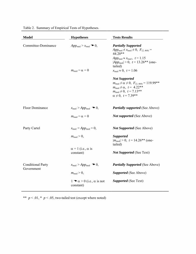
Table 2. Summary of Empirical Tests of Hypotheses. Model

Hypotheses

Tests Results

Committee-Dominance

Appmed > xmed 0, mmed = α = 0

Partially Supported Appmed ≠ xmed ≠ 0, F(2, 468) = 44.20** Appmed ≈ xmed , t = 1.15 |Appmed| > 0, t = 13.26** (one-tailed) xmed ≈ 0, t = 1.06 Not Supported mmed ≠ α ≠ 0, F(2, 468) = 119.99** mmed ≠ α, t = 4.22** mmed ≠ 0, t = 7.13** α ≠ 0, t = 7.39**

Floor Dominance

xmed > Appmed 0, mmed = α = 0

Partially supported (See Above) Not supported (See Above)

Party Cartel

xmed = Appmed = 0, mmed > 0, α = 1 (i.e., α is constant)

Not Supported (See Above) Supported |mmed| > 0, t = 14.26** (one-tailed) Not Supported (See Text)

Conditional Party Government

xmed > Appmed 0, mmed > 0, 1 α > 0 (i.e., α is not constant)

Partially Supported (See Above) Supported (See Above) Supported (See Text)

** p < .01, * p < .05, two-tailed test (except where noted)

Table 3a. Subcommittee Specific Models of Recommended House Appropriations, 1951 – 1998.a

Commerce, Justice,

State, and Judiciary

Independent

Variables

Treasury, P. O., &

Executive

Interior

Labor, Agriculture HEW

VA/HUD/ Independent

Offices

Constant 16078.56

64597.77

15145.53

14378.83

41009.88

88941.78

House Median - 18183.57 (0.71)

- 13405.81 (0.12)

- 16985.65 (0.75)

34768.58 (0.68)

- 72703.47 (1.55)

- 428515.21 (2.09)*

Majority Party Median

- 65767.12 - 297258.22 - 77122.09 (2.40)*

- 90513.02 (2.66)* (1.82) (1.25)

- 132183.35 (2.00)*

- 391065.52 (1.35)

Minority Party Median

- 33269.54 60929.29 (0.37)

8769.12 - 116069.56 (0.92) (0.27) (1.60)

3803.08 (0.06)

722290.00 (2.49)*

Median on Appropriations

2586.99 (0.29)

73103.17 (1.83)

471.60 (0.06)

99557.36 18211.63 (1.13)

16518.84 (0.23) (5.62)**

Maj. Party Med. on Approp.

131240.00 (5.44)**

450010.00 122000.00 21430.77 186840.00 (4.21)**

997450.00 (5.13)** (4.10)** (5.66)** (0.44)

Min. Party Med. on Approp.

72958.15 (2.38)*

128110.00 41664.59 (1.52)

89056.45 96152.27 (1.71)

- 88719.91 (0.36) (0.92) (1.44)

CPG

19755.98 (2.80)**

96466.66 19235.20 34155.46 (3.01)** (3.05)** (2.40)*

54611.65 (4.21)**

116810.00 (2.06)*

House Median × CPG

26039.71 - 75401.82 28774.25 - 211482.98 (0.65) (0.41) (0.80) (2.60)*

122950.00 (1.66)

606750.00 (1.87)

Majority Party Median × CPG

115190.00 418640.00 87018.06 287040.00 (1.81) (1.45) (1.53) (2.24)*

106250.00 (0.91)

405840.00 (0.79)

Minority Party Median × CPG

4284.79 - 234952.58 - 58913.11 197110.00 (0.07) (0.83) (1.06) (1.58)

- 129014.44 (1.13)

- 1238000.00 (2.48)*

Maj. Party Med. (Approp.) × CPG

- 176078.07 - 740516.86 - 167062.79 - 228337.37 (4.47)** (4.14)** (4.75)** (2.88)**

- 282073.32 (3.90)**

- 1367800.00 (4.31)**

Min. Party Med. (Approp.) × CPG

- 70742.55 - 139118.70 - 28251.24 - 192040.82 (1.41) (0.61) (0.63) (1.89)

- 97446.22 (1.05)

246420.00 (0.61)

Veto Pivot - 2902.80 (2.46)*

- 5487.69 (1.02)

- 2761.43 (2.62)*

511.72 (0.22)

- 6403.63 (2.95)**

- 16853.24 (1.77)

Post Reform 19880.61 75156.82 (5.51)**

13478.07 (5.03)**

18843.75 (6.63)** (3.12)**

41002.86 (7.44)**

- 20982.19 (0.87)

Post Reform - 43831.30 - 160004.45 - 30094.97 - 41289.88 (3.96)**

- 85718.38 (9.01)**

13887.51 (0.33) (8.48)** (6.80)** (6.51)** × CPG

Adj. R2 =

N = .93**

48 .85**

48 .93**

48 .21**

48 .93**

48 .57**

48

a Models are Fully Modified Ordinary Least Squares Regressions, t-Statistics in Parentheses. ** p < .01, * p < .05, two-tailed test

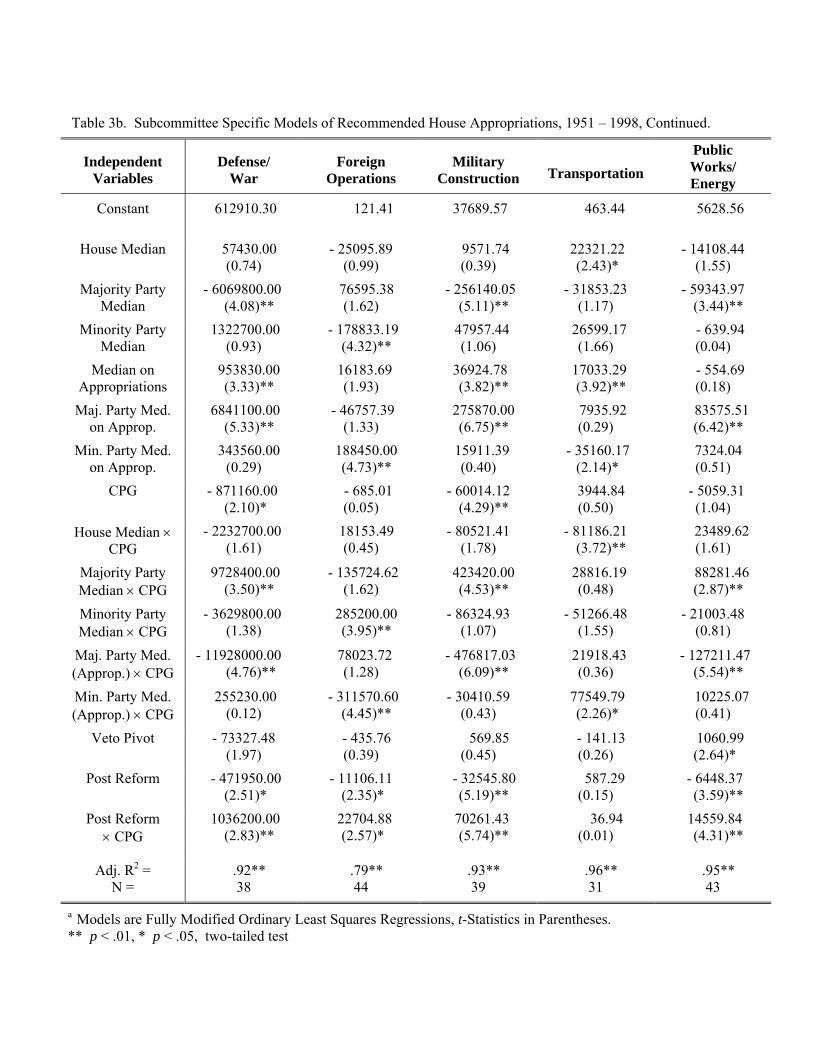
Table 3b. Subcommittee Specific Models of Recommended House Appropriations, 1951 – 1998, Continued.

Independent

Defense/

War

Foreign

Operations

Military

Variables Construction

Transportation

Public Works/ Energy

Constant 612910.30

121.41

37689.57

463.44

5628.56

House Median

57430.00 - 25095.89 9571.74 (0.39)

22321.22 (0.74) (0.99) (2.43)*

- 14108.44 (1.55)

Majority Party Median

- 6069800.00 76595.38 - 256140.05 (4.08)** (1.62) (5.11)**

- 31853.23 (1.17)

- 59343.97 (3.44)**

Minority Party Median

1322700.00 - 178833.19 (0.93) (4.32)**

47957.44 (1.06)

26599.17 (1.66)

- 639.94 (0.04)

Median on Appropriations

953830.00 16183.69 36924.78 (3.82)**

17033.29 (3.33)** (1.93) (3.92)**

- 554.69 (0.18)

Maj. Party Med. on Approp.

6841100.00 - 46757.39 275870.00 7935.92 (0.29)

83575.51 (5.33)** (1.33) (6.75)** (6.42)**

Min. Party Med. on Approp.

343560.00 (0.29)

188450.00 (4.73)**

15911.39 (0.40)

- 35160.17 (2.14)*

7324.04 (0.51)

CPG

- 871160.00 - 685.01 (2.10)* (0.05)

- 60014.12 (4.29)**

3944.84 (0.50)

- 5059.31 (1.04)

House Median × CPG

- 2232700.00 18153.49 - 80521.41 - 81186.21 (1.61) (0.45) (1.78) (3.72)**

23489.62 (1.61)

Majority Party Median × CPG

9728400.00 - 135724.62 423420.00 (3.50)** (1.62) (4.53)**

28816.19 (0.48)

88281.46 (2.87)**

Minority Party Median × CPG

- 3629800.00 285200.00 (3.95)**

- 86324.93 (1.07)

- 51266.48 (1.38) (1.55)

- 21003.48 (0.81)

Maj. Party Med. (Approp.) × CPG

- 11928000.00 (4.76)**

78023.72 (1.28)

- 476817.03 (6.09)**

21918.43 (0.36)

- 127211.47 (5.54)**

Min. Party Med. (Approp.) × CPG

255230.00 (0.12)

- 311570.60 (4.45)**

- 30410.59 (0.43)

77549.79 (2.26)*

10225.07 (0.41)

Veto Pivot - 73327.48 - 435.76 (0.39)

569.85 (0.45)

- 141.13 (1.97) (0.26)

1060.99 (2.64)*

Post Reform - 471950.00 - 11106.11 (2.35)*

- 32545.80 (5.19)**

587.29 (0.15)

- 6448.37 (3.59)** (2.51)*

Post Reform × CPG

1036200.00 (2.83)**

22704.88 (2.57)*

70261.43 (5.74)**

36.94 (0.01)

14559.84 (4.31)**

Adj. R2 = .92** .79** .93** .96** .95**

38 44 39 31 43 N = a Models are Fully Modified Ordinary Least Squares Regressions, t-Statistics in Parentheses. * * p < .01, * p < .05, two-tailed test

Figure 1a: Real Appropriations by Subcommittee and Fiscal Year (1951-1998).

0

50000000

100000000

150000000

200000000

250000000

300000000

350000000

400000000

450000000

1951

1953

1955

1957

1959

1961

1963

1965

1967

1969

1971

1973

1975

1977

1979

1981

1983

1985

1987

1989

1991

1993

1995

1997

Fiscal Year

Rea

l App

ropr

iatio

ns in

100

0s

TreasuryLaborInteriorAgricultureState, J,CHUDDefenseForeign OpnMilitary ConstructionTransportPublic Works

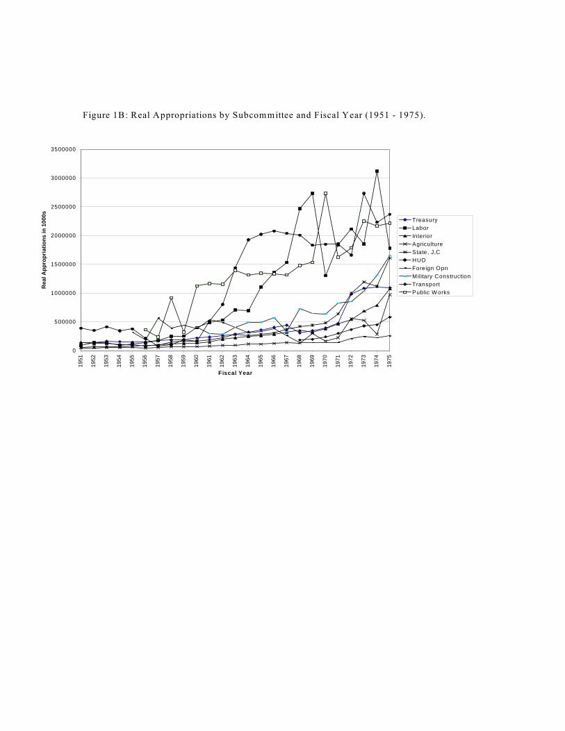
Figure 1B: Real Appropriations by Subcommittee and Fiscal Year (1951 - 1975).

0

500000

1000000

1500000

2000000

2500000

3000000

3500000

1951

1952

1953

1954

1955

1956

1957

1958

1959

1960

1961

1962

1963

1964

1965

1966

1967

1968

1969

1970

1971

1972

1973

1974

1975

Fiscal Year

Rea

l App

ropr

iatio

ns in

100

0s

TreasuryLaborInteriorAgricultureState, J,CHUDForeign OpnMilitary ConstructionTransportPublic Works

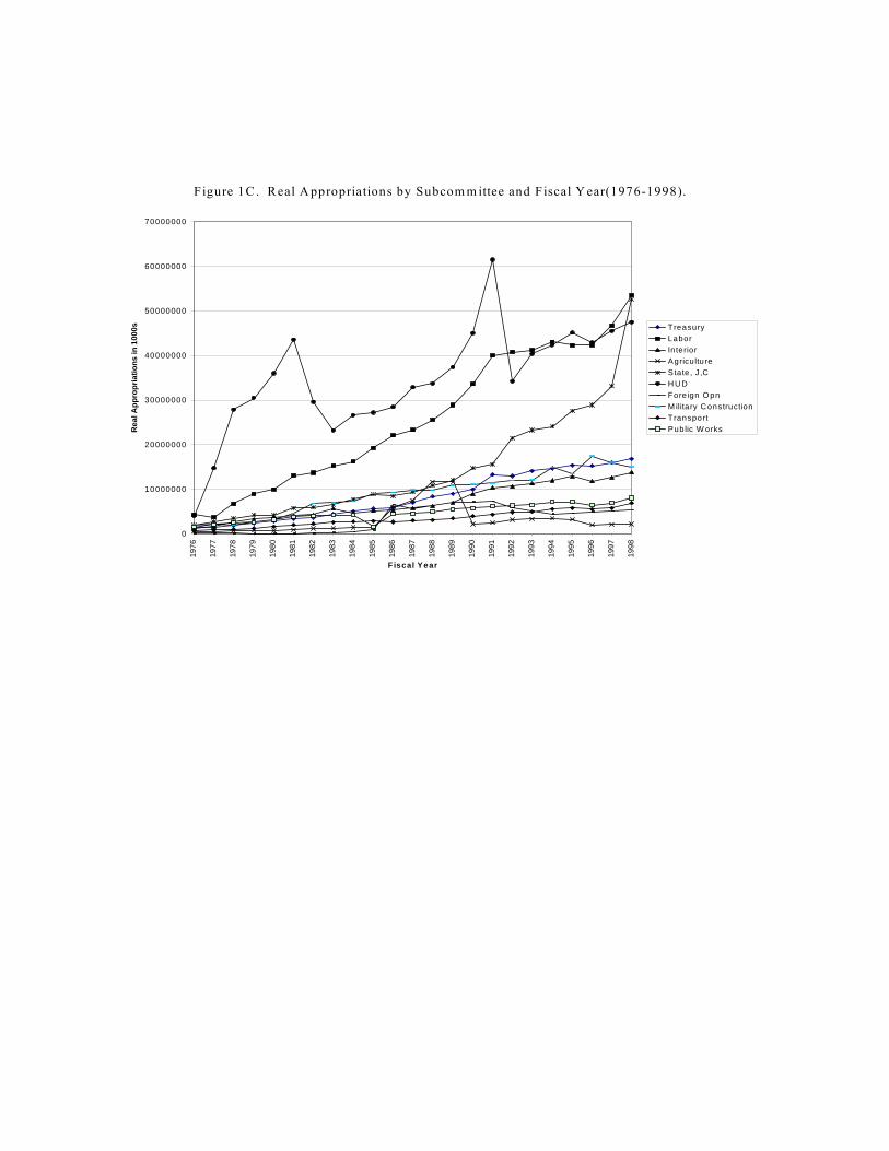
Figure 1C . Real A ppropriations by Subcom m ittee and Fiscal Y ear(1976-1998).

0

10000000

20000000

30000000

40000000

50000000

60000000

70000000

1976

1977

1978

1979

1980

1981

1982

1983

1984

1985

1986

1987

1988

1989

1990

1991

1992

1993

1994

1995

1996

1997

1998

Fiscal Year

Rea

l App

ropr

iatio

ns in

100

0s TreasuryLaborInteriorAgricultureState , J ,CHU DFore ign O pnM ilitary C onstructionTransportPublic W orks

Figure 2. Party Polarization in the U.S. House, 1876-1998

0

0.2

0.4

0.6

0.8

1

1.2

1876

1880

1884

1888

1892

1896

1900

1904

1908

1912

1916

1920

1924

1928

1932

1936

1940

1944

1948

1952

1956

1960

1964

1968

1972

1976

1980

1984

1988

1992

1996

Election Year

Con

ditio

nal P

arty

Gov

ernm

ent

Figure 3A. Median of the Floor, Majority Party, Minority Party, and Appropriations Committee over Time (1951-1998).

-0.6

-0.4

-0.2

0

0.2

0.4

0.6

0.8

1951

1953

1955

1957

1959

1961

1963

1965

1967

1969

1971

1973

1975

1977

1979

1981

1983

1985

1987

1989

1991

1993

1995

1997

Fiscal year

Nom

inat

e Sc

ore

House MedianMajority MedianMinority MedianCommittee Median

Figure 3B: Median of the Appropriations Committee as a Whole, of the Majority Party and Minority Party members on the Committee over Time (1951-1998).

-0.6

-0.4

-0.2

0

0.2

0.4

0.6

0.819

51

1953

1955

1957

1959

1961

1963

1965

1967

1969

1971

1973

1975

1977

1979

1981

1983

1985

1987

1989

1991

1993

1995

1997

Fiscal year

Nom

inat

e Sc

ore

Minority PartyMajority Party Committee Median

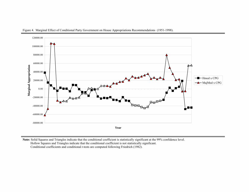
Figure 4. Marginal Effect of Conditional Party Government on House Appropriations Recommendations (1951-1998).

-80000.00

-60000.00

-40000.00

-20000.00

0.00

20000.00

40000.00

60000.00

80000.00

100000.00

120000.00

Year

Mar

gina

l App

ropr

iatio

n

Hmed x CPGMajMed x CPG

Note: Solid Squares and Triangles indicate that the conditional coefficient is statistically significant at the 99% confidence level. Hollow Squares and Triangles indicate that the conditional coefficient is not statistically significant. Conditional coefficients and conditional t-tests are computed following Friedrich (1982).