fokker-planck equations for a free energy...
TRANSCRIPT

FOKKER-PLANCK EQUATIONS FOR A FREE ENERGYFUNCTIONAL OR MARKOV PROCESS ON A GRAPH
SHUI-NEE CHOW, WEN HUANG, YAO LI AND HAOMIN ZHOU
Abstract. The classical Fokker-Planck equation is a linear parabolic equationwhich describes the time evolution of probability distribution of a stochastic pro-cess defined on an Euclidean space. Corresponding to a stochastic process, thereoften exists a free energy functional which is defined on the space of probabilitydistributions and is a linear combination of a potential and an entropy. In recentyears, it has been shown that the Fokker-Planck equation is the gradient flowof the free energy functional defined on the Riemannian manifold of probabilitydistributions whose inner product is generated by a 2-Wasserstein distance. Inthis paper, we consider analogous matters for a free energy functional or Markovprocess defined on a graph with a finite number of vertices and edges. If N ≥ 2is the number of vertices of the graph, we show that the corresponding Fokker-Planck equation is a system of N nonlinear ordinary differential equations definedon a Riemannian manifold of probability distributions. However, in contrast tostochastic processes defined on Euclidean spaces, the situation is more subtle fordiscrete spaces. We have different choices for inner products on the space of prob-ability distributions resulting in different Fokker-Planck equations for the sameprocess. It is shown that there is a strong connection but also substantial dis-crepancies between the systems of ordinary differential equations and the classicalFokker-Planck equation on Euclidean spaces. Furthermore, both systems of ordi-nary differential equations are gradient flows for the same free energy functionaldefined on the Riemannian manifolds of probability distributions with differentmetrics. Some examples will also be discussed.
1. Introduction
In this paper, we are concerned with the relationships among three conceptsdefined on graphs: the free energy functional, the Fokker-Planck equation and sto-chastic processes. We begin by recalling some of the well-known facts about them.
1991 Mathematics Subject Classification. 37H10,60J27,60J60.Key words and phrases. Markov process, Fokker-Planck equation, free energy, Gibbs density,
graph.The second author, Wen Huang, is partially supported by NSFC, Fok Ying Tung Education
Foundation and the Fundamental Research Funds for the Central Universities. The third author,Yao Li, is partially supported by NSF grant DMS0708331. The fourth author, Haomin Zhou, issupported in part by NSF Faculty Early Career Development (CAREER) Award DMS-0645266and DMS-1042998.
We would like to acknowledge the constructive comments and suggestions by the reviewer(s),and our communication with the editor, Professor D. Kinderlehrer. This paper would not becompleted without their help. We also want to thank Professors W. Gangbo and P. Tatali formany fruitful discussions on this subject.
1

2 SHUI-NEE CHOW, WEN HUANG, YAO LI AND HAOMIN ZHOU
Consider a stochastic process defined by the following randomly perturbed differ-ential equation,
(1.1) dx = −∇Ψ(x)dt+√
2βdWt, x ∈ RN ,
where Ψ(x) is a given scalar-valued potential function, β a positive constant, anddWt the white noise. This stochastic differential equation (SDE) is one of the pri-mary tools in many practical problems that involve uncertainty or incomplete infor-mation. Examples can be found in many different disciplines. Solutions of SDE’sare stochastic processes. The Fokker-Planck equation is a partial differential equa-tion describing the time evolution of the probability density function ρ(x, t) of thetrajectories of the SDE (1.1). It has the form
(1.2)∂ρ(x, t)
∂t= ∇ · (∇Ψ(x)ρ(x, t)) + β∆ρ(x, t),
where ∇ · (∇Ψ(x)ρ(x, t)) is called the drift term, and ∆ρ(x, t) is the diffusion termgenerated by white noise. The Fokker-Planck equation plays a prominent role inmany disciplines and has been studied by many authors (see, for example, [19, 44,46]).
The notion of free energy is widely used in many disciplines, and it is relatedto the maximal amount of work that can be extracted from a system ([33, 47, 54]and references therein). For us, a free energy functional is a scalar-valued functiondefined on the space of probability distributions and is composed of a potentialenergy U and an entropy functional S, i.e. the free energy is expressed as
(1.3) F (ρ) = U(ρ)− βS(ρ),
where β > 0 is a constant called temperature, and ρ is a probability density functiondefined on a state space X, which may be “continuous” (e.g. X = RN), or “discrete”(e.g. X = {a1, · · · , aN}). For a system with state space RN , the potential functionalis defined by
U(ρ) :=
∫RN
Ψ(x)ρ(x)dx,
where Ψ(x) is a given potential function. The entropy, also called Gibbs-Boltzmannentropy, is given by
S(ρ) := −∫
RNρ(x) logρ(x)dx.
It is well known that the global minimizer of the free energy F is a probabilitydistribution, called Gibbs distribution,
(1.4) ρ∗(x) =1
Ke−Ψ(x)/β, where K =
∫RNe−Ψ(x)/β dx.
We note that in order for equation (1.4) to be well-defined, Ψ must satisfy somegrowth condition to ensure that K is finite. In this paper, we consider only potentialssatisfying this condition.
Although historical developments of the free energy and Fokker-Planck equationare not directly related, there are many studies that reveal some connection between

FOKKER-PLANCK EQUATION ON THE GRAPHS 3
them. The following two results about the relationship between them are well known[15, 17, 19, 25, 26, 35, 44]:
(1) The free energy (1.3) is a Lyapunov functional for the Fokker-Planck equa-tion (1.2), i.e., if the probability density ρ(t, x) is a solution of (1.2), thenF (ρ(t, x)) is a decreasing function of time.
(2) The Gibbs distribution (1.4) is the global minimizer of the free energy (1.3)and is the unique stationary solution of the Fokker-Planck equation (1.2).
In recent years, there have been many studies about the connection between thefree energy, the Fokker-Planck equation, the Ricci curvature, and optimal trans-portation in a continuous state space. For example, Jordan, Kinderlehrer and Otto[25, 35] showed that the Fokker-Planck equation may be viewed as the gradientflow of the free energy functional on a Riemannian manifold of probability measureswith a 2-Wasserstein metric. More precisely, let the state space X be a “suitable”complete metric space with distance d, and P(X) be the space of Borel probabil-ity measures on X. For any given two elements µ1, µ2 ∈ P(X), the 2-Wassersteindistance between µ1 and µ2 is defined by
(1.5) W2(µ1, µ2)2 = infλ∈M(µ1,µ2)
∫X×X
d(x, y)2dλ(x, y),
where M(µ1, µ2) is the collection of Borel probability measures on X × X withmarginal measures µ1 and µ2 respectively. Then (P(X),W2) forms a Riemannianmanifold and the Fokker-Planck equation (1.2) can be derived by an implicit schemewhich can be reinterpreted as a gradient flow of the free energy (1.3) on this manifold.Clearly, we have two metric spaces (X, d) and (P(X),W2), and there exists anisometric embedding X → P(X) given by x → δx. For the notion of Wassersteindistance, we refer to [13, 53]. For theory and applications of the Wasserstein distance,we refer to the articles [2, 8, 9, 10, 16, 18, 31, 36, 51, 52] and references therein.
We note that Otto and Westdickenberg [37] showed the relationship between 2-Wasserstein distance and minimal energy curves on X = RN . Moreover, the con-vexity of the entropy on (P(X),W2) is equivalent to the non-negativity of the Riccicurvature, which induces the definition of the abstract Ricci curvature on lengthspaces [12, 42, 43, 48, 49, 50]. Furthermore, it is proved in [32] that if (X, d) is alength space, then the manifold (P(X),W2) is also a length space.
We summarize that the relationship among the free energy, the Fokker-Planckequation and stochastic processes in the state space RN in Figure 1. From the freeenergy point of view, the Fokker-Planck equation is the gradient flow of the freeenergy on the probability space with 2-Wasserstein metric. From the viewpoint ofstochastic processes, the Fokker-Planck equation describes the time evolution of theprobability density function.
In this paper, we consider similar matters on a discrete state space which is afinite graph. For a system with a discrete state space X = {a1, a2, · · · , aN}, we letρ = {ρi}Ni=1 be a probability distribution on X, i.e.,
N∑i=1
ρi = 1 ρi ≥ 0,

4 SHUI-NEE CHOW, WEN HUANG, YAO LI AND HAOMIN ZHOU
Figure 1. Interrelations among the free energy, Fokker-Planck equa-tion and the stochastic differential equation in RN .
where ρi is the probability of state ai. Then the free energy functional has thefollowing expression:
(1.6) F (ρ) =N∑i=1
Ψiρi + βN∑i=1
ρi log ρi,
where Ψi is the potential at the state ai. Obviously, the potential and entropyfunctionals are given respectively by
U(ρ) :=N∑i=1
Ψiρi, and S(ρ) := −N∑i=1
ρi log ρi.
The free energy functional has a global minimizer, the Gibbs density, given by
(1.7) ρ∗i =1
Ke−Ψi/β, where K =
N∑i=1
e−Ψi/β.
Despite remarkable development in the theory related to Fokker-Planck equationin continuous state spaces, much less is known when the state space is discrete andfinite. There are results in mass transport theory for discrete spaces [4, 34, 45].However, to the best of our knowledge, the Fokker-Planck equation on a graph hasnot been established. We know that a finite metric space with more than one pointis not a length space. This indicates that existing theory may not be extendeddirectly to a finite graph. In addition, the notion of “white noise” is also not clearfor a Markov process defined on a graph.
Based on recent results in continuous state spaces, it is natural to apply spa-tial discretization schemes, such as the central difference scheme, to Fokker-Planckequation (1.2) to obtain their counterparts for discrete state spaces. The result-ing equation for a discrete state space is a system of ordinary differential equations.However, many problems arise with this approach. For instance, commonly used lin-ear discretization schemes often lead to steady states that are different from Gibbsdensity (1.7), which is the global minimizer of the free energy. In fact, we proverigorously that no linear discretization scheme could achieve the Gibbs distribu-tion at its steady state for general potentials in Theorem 2.1. This suggests that

FOKKER-PLANCK EQUATION ON THE GRAPHS 5
the equation obtained by a linear discretization scheme does not capture the realenergy landscape of the free energy on a discrete space, and it is not the desiredFokker-Planck equation.
Inspired by Figure 1, we define the Fokker-Planck equation on a graph X bytwo different strategies. From the free energy viewpoint, since there is no readysubstitute for the Wasserstein metric on a graph, we first endow the probabilityspace P(X) with a Riemannian metric d, which depends on the potential as well asthe structure of the graph. Then, the Fokker-Planck equation can be derived as thegradient flow of the free energy F on the Riemannian manifold (P(X), d). Fromthe stochastic process viewpoint, we introduce a new interpretation of white noiseperturbations to a Markov process on X, and derive another Fokker-Planck equationas the time evolution equation for its probability density function. We must notethat unlike the continuous state space case, we obtain two different Fokker-Planckequations on the graph following these approaches. It seems one of the reasonsthat we obtain different Fokker-Planck equations is that finite graphs are not lengthspaces generally.
To be more precise on the approaches, we consider a graph G = (V,E), whereV = {a1, · · · , aN} is the set of vertices, and E the set of edges. We denote theneighborhood of a vertex ai ∈ V by N(i):
N(i) = {j ∈ {1, 2, · · · , N}|{ai, aj} ∈ E}.We further assume that the graph G is a simple graph (i.e., there are no self loopsor multiple edges) with |V | ≥ 2, and G is connected. We note that results in thispaper still hold after nominal modifications if the graph G is not simple.
Let Ψ = (Ψi)Ni=1 be a given potential function on V , where Ψi is the potential on
ai. β ≥ 0 is the strength of “white noise”. Let
M =
{ρ = (ρi)
Ni=1 ∈ RN |
N∑i=1
ρi = 1 and ρi > 0 for i = 1, 2, · · · , N
},
be the space of positive probability distributions on V . Then from the free energyviewpoint, we obtain a Fokker-Planck equation on M (see Theorem 4.1) :
dρidt
=∑
j∈N(i),Ψj>Ψi
((Ψj + β log ρj)− (Ψi + β log ρi))ρj
+∑
j∈N(i),Ψj<Ψi
((Ψj + β log ρj)− (Ψi + β log ρi))ρi
+∑
j∈N(i),Ψj=Ψi
β(ρj − ρi)
(1.8)

6 SHUI-NEE CHOW, WEN HUANG, YAO LI AND HAOMIN ZHOU
for i = 1, 2 · · · , N . If we take the stochastic process viewpoint, then we obtain adifferent Fokker-Planck equation on M (see Theorem 5.2) :
dρidt
=∑
j∈N(i),Ψj>Ψi
((Ψj + β log ρj)− (Ψi + β log ρi))ρj
+∑
j∈N(i),Ψj<Ψi
((Ψj + β log ρj)− (Ψi + β log ρi))ρi
(1.9)
where Ψi = Ψi + β log ρi and i = 1, 2, · · · , N . For convenience, we call equations(1.8) and (1.9) Fokker-Planck equation I (1.8) and II (1.9) respectively.
We will show that Fokker-Planck equation I (1.8) is the gradient flow of free energy(1.6) on a Riemannian manifold (M, dΨ), where dΨ is a Riemannian metric on Minduced by Ψ, and we will give the precise definition of (M, dΨ) in Section 3. Onthe other hand, Fokker-Planck equation II (1.9) is derived from a Markov processon G subject to a “white noise” perturbation, for which we will give the definitionin Section 5. In the continuous case, the Fokker-Planck equation obtained by thesetwo different strategies coincides beautifully. However, in the discrete case, thereare substantial differences between them, although their appearances seem to differonly a little. The connection of Fokker-Planck equation I (1.8) to a Markov processon the graph is still unclear. Fokker-Planck equation II (1.9) is not a gradient flow ofthe free energy on a smooth Riemannian manifold of the probability space. However,it is a “gradient flow” of the free energy on another metric space (M, dΨ), which isonly piecewise smooth. More precisely, we will show thatM is divided into a finitenumber of segments, and dΨ is only smooth in the interior of each segment. We alsonote that the manner we derive Fokker-Planck equation II (1.9) seems to be relatedto Onsager’s flux [39, 40, 41].
Although (1.8) and (1.9) are different, they share some similar properties forβ > 0:
• Free energy F decreases along solutions of both equations.• Both equations are gradient flows of the same free energy on the same prob-
ability space M, but with different metrics.• The Gibbs distribution ρ∗ = (ρ∗i )
Ni=1 is the stable stationary solution of both
equations.• Near the Gibbs distribution, the difference between the two equations is
small.• For both equations, given any initial condition ρ0 ∈M, there exists a unique
solution ρ(t,ρ0) for t ≥ 0, and ρ(t,ρ0)→ ρ∗, as t→ +∞.
Formally, if the graph is a lattice, both Fokker-Planck equation I (1.8) and II (1.9)can be viewed as special upwind numerical schemes of the Fokker-Planck equation onthe continuous state space (1.2). However, they are both uncommonly used schemes.In particular, the diffusion term is discretized by two surprisingly consistent non-linear schemes, which, to the best of our knowledge, have not been considered byother authors. It is worth mentioning that most of the commonly used consistent

FOKKER-PLANCK EQUATION ON THE GRAPHS 7
and stable linear schemes, such as central difference scheme, lead to unexpectedproblems as demonstrated in Section 2.
The results obtained in this paper are largely inspired by recent developmentsin the Fokker-Planck equation and the 2-Wasserstein metric, especially the theoryreported in [25, 26, 35]. Our results are also influenced by the upwind schemesfor shock capturing in conservation laws [6, 29], as well as the recent studies onParrondo’s paradox [22, 23] and flashing ratchet models for molecular motors [1,14, 24]. We will demonstrate a Parrondo’s paradox of free energy by applying ourFokker-Planck equation (1.8) to a flashing ratchet model.
During the time when this paper was under review, we found that Mielke in-troduced a Riemannian metrics independently in [28], which is similar to our Rie-mannian metrics with a constant potential. More precisely, if we express a chemicalreaction system as a graph, then Mielke’s metric can be obtained by discretizingOtto’s calculus in a way similar to ours. Mielke studied reaction-diffusion equationwith his metric, showed that a reaction-diffusion equation with detailed balancecould be written as a gradient flow of relative entropy. More recently, Qian et al.[20] gives an interesting physical explanation of the log-average term
ρi − ρjlog ρi − log ρj
which appear in both our and Mielke’s metrics. We cite from [20] that the log-averageis the“conductance in the stoichiometric network theory of chemical reactions”, and“the numerator is the flux and the denominator is the driving force of a transi-tion”. These new progress reveals some potential connections between our work andchemical reactions.
This paper is organized as follows: In Section 2, we discuss why we must use non-linear Fokker-Planck equations in the discrete case. Some basic geometric propertiesof M are shown in Section 3. In Section 4, we prove that Fokker-Planck equationI (1.8) is the gradient flow of free energy, and show some related properties. InSection 5, we show how we interpret “white noise” in the Markov process to obtainFokker-Planck equation II (1.9). In Section 6, we explain the upwind structure inFokker-Planck equations I (1.8) and II (1.9). In the last section, we consider theflashing ratchet model as an application.
2. Why Nonlinear Fokker-Planck Equations on Graphs
Comparing the Fokker-Planck equation (1.2) in the continuous state space withour Fokker-Planck equations (1.8) and (1.9) on graphs, one immediately noticesthat our equations are nonlinear while (1.2) is linear. It is natural to questionthe nonlinearity in both equations. For example, can one just apply common dis-cretization schemes, such as the well known central difference, to (1.2) and obtainlinear Fokker-Planck equations in the discrete case? However, in our numerical stud-ies, we encountered many problems. For instance, steady state solutions of linearequations derived from discretization are not the Gibbs distributions. Furthermore,the free energy does not decay along the solutions. In this section, we prove that

8 SHUI-NEE CHOW, WEN HUANG, YAO LI AND HAOMIN ZHOU
these problems occur for all linear systems obtained from discretizing the continuousFokker-Planck equation (1.2) using consistent linear schemes.
To be more precise, any given linear discretization of (1.2) can be written as
(2.1)dρidt
=∑j
((∑k
eijkΨk) + cij)ρj, for i = 1, 2, · · · , N,
where Ψ is the given potential and {eijk}N×N and {cij}N are some constants that arenot all zero. Assume that the Gibbs distribution (1.7) is the steady state solutionof (2.1), then we must have
(2.2)∑j
((∑k
eijkΨk) + cij)e−
Ψjβ = 0, for i = 1, 2, · · · , N.
Let us denote A as the collection of potentials Ψ satisfying (2.2), i.e.
(2.3) A = {(Ψ1, · · · ,ΨN) ∈ RN :∑j
((∑k
eijkΨk) + cij)e−
Ψjβ = 0, for 1 ≤ i ≤ N}.
Theorem 2.1. The set A has zero measure in RN , i.e.
κ(A) = 0,
where κ(·) is the Lebesgue measure on RN .
To prove this theorem, we need the following lemma.
Lemma 2.2. Let g(x) be a function in C1(RN). Denote B = {x ∈ RN : g(x) = 0},and Bj = {x ∈ B : gxj(x) = 0} for j = 1, · · · , N . Then
(2.4) κ(Bj) = κ(B).
Proof. This lemma is a special case of a well known fact about functions in Sobolevspaces, see for example, Lemma 7.7 in [21]. �
Now, we are ready to prove Theorem 2.1.
Proof. For the convenience of notations, let us denote Ψ = (Ψ1, · · · ,ΨN) and
fi(Ψ) =∑j
((∑k
eijkΨk) + cij)e−
Ψjβ .
Clearly, we have fi ∈ C∞(RN). Then, we can consider the sets, Aϑ, which collectall potentials Ψ ∈ A with vanishing ϑ-th derivatives of fi for all i = 1, · · · , N , thatis
Aϑ = {Ψ ∈ A : Dϑfi(Ψ) = 0, for 1 ≤ i ≤ N},where ϑ = (ϑ1, · · · , ϑN) is a multiple non-negative integer index, and Dϑ is thepartial derivative operator. Obviously, A and Aϑ are closed subsets.
Using Lemma 2.2 recursively, we have
(2.5) κ(A) = κ(Aϑ),
for arbitrary multi-index ϑ. Next, we show κ(A) = 0 by contradiction.

FOKKER-PLANCK EQUATION ON THE GRAPHS 9
Assume that κ(A) > 0, so we have κ(Aϑ) = κ(A) > 0 for arbitrary multi-indexϑ. This implies that there must exist a potential Ψ0 ∈ A such that
fi(Ψ0) = 0 and Dϑfi(Ψ
0) = 0,
for arbitrary ϑ.For any r ∈ {1, · · · , N} and s ∈ {1, · · · , N} with r 6= s, we have
∂3fi∂Ψ2
r∂Ψs
(Ψ) =eirsβ2e−
Ψrβ .
Therefore,∂3fi
∂Ψ2r∂Ψs
(Ψ0) = 0
implies eirs = 0 for r 6= s. Thus, we must have
fi(Ψ) =∑j
(eijjΨj + cj)e−
Ψjβ .
It is easy to compute that for any j ∈ {1, · · · , N},∂lfi∂Ψl
j
=
(leijj
(−β)l−1+
(eijjΨj + cij)
(−β)l
)e−
Ψjβ ,
for arbitrary l ∈ N. Using the fact that
∂lfi∂Ψl
j
(Ψ0) = 0,
which is−βleijj + (eijjΨ
0j + cij) = 0, for all l ≥ 1.
This implies eijj = 0 and cij = 0, and it contradicts to the fact that not all of eijk and
cij are zero. So we must have κ(A) = 0. �
Theorem 2.1 indicates that one can not expect a linear system obtained by aconsistent discretization of the continuous Fokker-Planck equation (1.2) to achievethe Gibbs distribution at its steady state for general potentials. It suggests that aFokker-Planck equation on a graph needs to be nonlinear in general. However, thisdoes not imply that general linear systems can not achieve the Gibbs distribution attheir steady states. In fact, it can be verified that for any given probability vectorρ∗, including the Gibbs distribution, there exists a “reaction matrix” A, such thatthe solution of the ODE system
ρ′(t) = ρA
tends to ρ∗ as time t → ∞. Furthermore, the choice of A is not unique. One maychoose any A with the property of eAt → P , where P = [ρ∗, ρ∗, · · · , ρ∗] is a rankone matrix. For example, taking A = P − I will work in this situation. But such amatrix A can not be obtained by linearly discretizing the continuous Fokker-Planckequation in a consistent way as we explained in Theorem 2.1.

10 SHUI-NEE CHOW, WEN HUANG, YAO LI AND HAOMIN ZHOU
3. Metrics on M and Riemannian manifold
Given a graph G = (V,E) with V = {a1, a2, · · · , aN}, we consider all positiveprobability distributions on V :
M =
{ρ = (ρi)
Ni=1 ∈ RN |
N∑i=1
ρi = 1 and ρi > 0 for i ∈ {1, 2, · · · , N}
},
and its closure,
M =
{ρ = (ρi)
Ni=1 ∈ RN |
N∑i=1
ρi = 1 and ρi ≥ 0 for i ∈ {1, 2, · · · , N}
}.
Let ∂M be the boundary of M, i.e.
∂M =
{ρ = {ρi}Ni=1 ∈ RN |
N∑i=1
ρi = 1, ρi ≥ 0 andN∏i=1
ρi = 0
}.
The tangent space TρM at ρ ∈M is defined by
TρM =
{σ = (σi)
Ni=1 ∈ RN |
N∑i=1
σi = 0
}.
It is clear that the standard Euclidean metric on RN , d, is also a Riemannian metricon M.
Let
(3.1) Φ : (M, d)→ (RN , d)
be an arbitrary smooth map given by:
Φ(ρ) = (Φi(ρ))Ni=1, ρ ∈MIn the following, we will endow M with a metric dΦ, which depends on Φ and thestructure of G.
For technical reasons, we first consider the function
r1 − r2
log r1 − log r2
where r1 > 0, r2 > 0 and r1 6= r2. We want to extend it to the closure of the firstquadrant in the plane. In fact, this can be easily achieved by the following function:
e(r1, r2) =
r1−r2
log r1−log r2if r1 6= r2 and r1r2 > 0
0 if r1r2 = 0
r1 if r1 = r2
.
It is easy to check that e(r1, r2) is a continuous function on
{(r1, r2) ∈ R2 : r1 ≥ 0, r2 ≥ 0}and satisfies
min{r1, r2} ≤ e(r1, r2) ≤ max{r1, r2}.

FOKKER-PLANCK EQUATION ON THE GRAPHS 11
For simplicity, we will use its original form instead of the function e(r1, r2) in thispaper.
Next, we introduce the following equivalence relation “∼ ” in RN :
p ∼ q if and only if p1 − q1 = p2 − q2 = · · · = pN − qN ,and let W be the quotient space RN/ ∼. In other words, for p ∈ RN we considerits equivalent class
[p] = {(p1 + c, p2 + c, · · · , pN + c) : c ∈ R},and all such equivalent classes form the vector space W .
For a given Φ, and [p] = [(pi)Ni=1] ∈ W , we define an identification τΦ([p]) =
(σi)Ni=1 from W to TρM by,
(3.2) σi =∑j∈N(i)
ΓΦij(ρ)(pi − pj),
where
(3.3) ΓΦij(ρ) =
ρi if Φi > Φj, j ∈ N(i)ρj if Φj > Φi, j ∈ N(i)
ρi−ρjlog ρi−log ρj
if Φi = Φj, j ∈ N(i)
for i = 1, 2, · · · , N . With this identification, we can express σ ∈ TρM by [p] :=τ−1Φ (σ) ∈ W , and denoted it by
σ ' [(pi)Ni=1].
We note that this identification depends on Φ, the probability distribution ρ and thestructure of the graph G. In the following lemma, we show that this identification(3.2) is well defined.
Lemma 3.1. If each σi satisfies (3.2), then the map τΦ : [(pi)Ni=1] ∈ W 7→ σ =
(σi)Ni=1 ∈ TρM is a linear isomorphism.
Proof. It is clear that
τΦ : [(pi)Ni=1] ∈ W 7→ τΦ([(pi)
Ni=1]) = (σi)
Ni=1 ∈ TρM
is a well-defined linear map. Furthermore, bothW and TρM are (N−1)-dimensionalreal linear spaces. Thus, in order to prove the map τΦ is an isomorphism, it issufficient to show that the map τΦ is injective, which is equivalent to the fact thatif p = {pi}Ni=1 ∈ RN satisfies
σi =∑j∈N(i)
ΓΦij(pi − pj) = 0,⇐⇒ pi =
∑j∈N(i)
ΓΦijpj
/
∑j∈N(i)
ΓΦij
for i = 1, 2, · · · , N , then p1 = p2 = · · · = pN .
Assume this is not true, and let c = max{pi : i = 1, 2, · · · , N}. Then, there mustexists {a`, ak} ∈ E such that p` = c and pk < c, because the graph G is connected.

12 SHUI-NEE CHOW, WEN HUANG, YAO LI AND HAOMIN ZHOU
This gives
c = p` =
∑j∈N(`) ΓΦ
`jpj∑j∈N(`) ΓΦ
`j
= c+
∑j∈N(`) ΓΦ
`j(pj − c)∑j∈N(`) ΓΦ
`j
≤ c− ΓΦ`k(c− pk)∑j∈N(`) ΓΦ
`j
< c,
which is a contradiction. The proof is complete. �
Definition 3.2. By the above identification (3.2), we define an inner product onTρM by:
gΦρ (σ1,σ2) =
N∑i=1
p1iσ
2i =
N∑i=1
p2iσ
1i .
It is easy to check that this definition is equivalent to
(3.4) gΦρ (σ1,σ2) =
∑{ai,aj}∈E
ΛΦij(p
1i − p1
j)(p2i − p2
j),
where
(3.5) ΛΦij(ρ) =
{ρj if {ai, aj} ∈ E,Φi < Φj,
ρi−ρjlog ρi−log ρj
if {ai, aj} ∈ E,Φi = Φj,
for σ1 = (σ1i )Ni=1,σ
2 = (σ2i )Ni=1 ∈ TρM, and [(p1
i )Ni=1], [(p2
i )Ni=1] ∈ W satisfying
σ1 ' [(p1i )Ni=1] and σ2 ' [(p2
i )Ni=1].
In particular,
(3.6) gΦρ (σ,σ) =
∑{ai,aj}∈E
ΛΦij(ρ)(pi − pj)2
for σ ∈ TρM, where σ ' [(pi)Ni=1].
Since ρ ∈M 7→ gΦρ is measurable, using the inner product gΦ
ρ , we can define the
distance between two points ρ1 and ρ2 in M by
(3.7) dΦ(ρ1,ρ2) = infγL(γ(t))
where γ : [0, 1] →M ranges over all continuously differentiable curve with γ(0) =ρ1, γ(1) = ρ2. The arc length of γ is given by
L(γ(t)) =
∫ 1
0
√gΦγ(t)(γ(t), γ(t))dt.
Although gΦρ may or may not be a smooth inner product with respect to ρ, the
length of any smooth curve is still well defined because ρ ∈M 7→ gΦρ is measurable.
It is shown by Lemma 3.4 that dΦ is a metric on M. Thus we have a metricspace (M, dΦ). In particular, if Φ is a constant map, then the metric dΦ is aRiemannian metric on M since the map ρ ∈ M 7→ gΦ
ρ is smooth. Hence, (M, dΦ)is a Riemannian manifold.

FOKKER-PLANCK EQUATION ON THE GRAPHS 13
Remark 3.3. The identification (3.2) is motivated by a similar identification intro-duced by F. Otto in [35] for the case of a continuous state space. We replace thedifferential operator in [35] by a combination of finite differences because our statespace V is discrete. Since (3.2) adopts an upwind scheme and the structure of Kol-mogorov equation (5.1) in Section 5, we call the inner product gΦ
ρ the upwind innerproduct induced by Φ.
Next, we show that the metric dΦ is bounded. Given ρ = (ρi)Ni=1 ∈M, we define
matrices
A = [A(i, j)]N×N , Am = [Am(i, j)]N×N , and AM = [AM(i, j)]N×N
as follows. If i 6= j, we have
A(i, j) =
{−ΓΦ
ij(ρ) if {ai, aj} ∈ E0 otherwise
,
Am(i, j) =
{−max{ρi, ρj} if {ai, aj} ∈ E0 otherwise
and
AM(i, j) =
{−min{ρi, ρj} if {ai, aj} ∈ E0 otherwise
.
On the diagonal, i = j, we defineA(i, i) = −
∑k 6=i
A(i, k)
Am(i, i) = −∑k 6=i
Am(i, k)
AM(i, i) = −∑k 6=i
AM(i, k)
.
Thus the identification (3.2) can be expressed by
σT = ApT
where σ = (σi)Ni=1 ∈ TρM and p = (pi)
Ni=1 ∈ RN .
We consider two new identifications
(3.8) σT = AmpT
and
(3.9) σT = AMpT .
Similar to the identification (3.2), identifications (3.8) and (3.9) are both linear iso-morphisms between TρM and W . Furthermore, they induce inner products gmρ (·, ·)and gMρ (·, ·) respectively on TρM. It is not hard to see that the maps ρ 7→ gmρand ρ 7→ gMρ are smooth. By using the inner products gmρ and gMρ , we can obtaindistances dm(·, ·) and dM(·, ·) respectively onM. Then both (M, dm) and (M, dM)are smooth Riemannian manifolds.

14 SHUI-NEE CHOW, WEN HUANG, YAO LI AND HAOMIN ZHOU
Lemma 3.4. For any smooth map Φ : (M, d)→ (RN , d) and ρ1,ρ2 ∈M,
dm(ρ1,ρ2) ≤ dΦ(ρ1,ρ2) ≤ dM(ρ1,ρ2).
Proof. Let Φ : (M, d)→ (RN , d) be a smooth map. Given ρ ∈M, the identification(3.2) can be expressed by
σT = ApT
where σ = (σi)Ni=1 ∈ TρM and p = (pi)
Ni=1 ∈ RN . Since
∑Ni=1 σi = 0 for
(σi)Ni=1 ∈ TρM, by deleting the last row and last column of the matrix A we obtain a
symmetric diagonally dominant (N−1)×(N−1)-matrix B. Thus, the identification(3.2) becomes
σT∗ = BpT∗where σ∗ = (σi)
N−1i=1 and p∗ = (pi − pN)N−1
i=1 .Similarly we can get symmetric diagonally dominant matrices Bm and BM from
Am and AM respectively. Moreover, B, Bm and BM are all irreducible matrices sincethe graph G is connected. They are all nonsingular and positive definite, becausethey all have positive diagonal entries.
The inner products are given as
gΦρ (σ,σ) = σpT = σ∗p
T∗ = σ∗B
−1σT∗
gmρ (σ,σ) = σpT = σ∗pT∗ = σ∗B
−1m σ
T∗
gMρ (σ,σ) = σpT = σ∗pT∗ = σ∗B
−1M σ
T∗
for σ ∈ TρM. It is well known that a symmetric diagonally dominant real matrixwith nonnegative diagonal entries is positive semidefinite. Since Bm − B, B − BM
are still symmetric diagonally dominant matrices with nonnegative diagonal entries,we have Bm − B and B − BM are positive semidefinite. Now we claim that: forevery σ ∈ TρM, we have
gmρ (σ,σ) ≤ gΦρ (σ,σ) ≤ gMρ (σ,σ).
We first provegmρ (σ,σ) ≤ gΦ
ρ (σ,σ).
Note thatgΦ
ρ (σ,σ)− gmρ (σ,σ) = σ∗(B−1 −B−1
m )σT∗ .
Therefore, to show thatgmρ (σ,σ) ≤ gΦ
ρ (σ,σ),
it is sufficient to show (B−1 −B−1m ) is positive semi-definite.
Since B is a positive definite symmetric matrix, B−1 is also positive definitesymmetric. Combining this with the fact that (Bm − B) is positive semi-definite,we know that (B−1 −B−1
m ) is positive semi-definite from the following equality
B−1 −B−1m = B−1
m {(Bm −B)B−1(Bm −B)T + (Bm −B)}(B−1m )T .
In a similar fashion, we prove gΦρ (σ,σ) ≤ gMρ (σ,σ).
Thus we obtaindm(ρ1,ρ2) ≤ dΦ(ρ1,ρ2) ≤ dM(ρ1,ρ2)
for any ρ1,ρ2 ∈M. �

FOKKER-PLANCK EQUATION ON THE GRAPHS 15
Now we consider two choices of the function Φ which are related to Fokker-Planckequation I (1.8) and II (1.9) respectively. Let the potential Ψ = (Ψi)
Ni=1 on V be
given and β ≥ 0, where Ψi is the potential on vertex ai.For Fokker-Planck equation I (1.8), we let
Φ(ρ) ≡ Ψ,
where ρ ∈M. The identification (3.2)
σ ' [(pi)Ni=1]
is given by
(3.10) σi =∑j∈N(i)
(pi − pj)ΓΨij (ρ)
and the corresponding norm (3.6) is
(3.11) gΨρ (σ,σ) =
∑{ai,aj}∈E
ΛΨij (ρ)(pi − pj)2,
for σ ∈ TρM with σ ' [(pi)Ni=1]. Note that the map ρ ∈M 7→ gΨ
ρ is smooth and the
inner product gΨ generates a Riemannian metric space (M, dΨ), where dΨ comesfrom (3.7). Similar to the theory developed in [35], we will show in Section 4 thatFokker-Planck equation I (1.8) is the gradient flow of free energy on the Riemannianmanifold (M, dΨ).
For Fokker-Planck equation II (1.9), we let
Φ(ρ) ≡ Ψ(ρ),
where the new potential Ψ(ρ) = (Ψi(ρ))Ni=1 is defined by
Ψi(ρ) = Ψi + β log ρi.
In this case, for a given ρ ∈M, the identification (3.2) is given by
(3.12) σi =∑j∈N(i)
(pi − pj)ΓΨij (ρ),
and the inner product (3.4) on TρM is
(3.13) gΨρ (σ1,σ2) =
N∑i=1
p1iσ
2i =
N∑i=1
p2iσ
1i =
∑{ai,aj}∈E
ΛΨij (ρ)(p1
i − p1j)(p
2i − p2
j),
for σ1 = (σ1i )Ni=1,σ
2 = (σ2i )Ni=1 ∈ TρM, and [(p1
i )Ni=1], [(p2
i )Ni=1] ∈ W satisfying σ1 '
[(p1i )Ni=1] and σ2 ' [(p2
i )Ni=1]. In particular, we have
(3.14) gΨρ (σ,σ) =
∑{ai,aj}∈E
ΛΨij (ρ)(pi − pj)2,
for σ ∈ TρM and σ ' [(pi)Ni=1].
The inner product gΨρ induces a metric space (M, dΨ), where dΨ comes from
(3.7). However, the map ρ ∈ M 7→ gΨρ is not continuous due to the fact that Ψ
depends on ρ. Thus, (M, dΨ) is not a Riemannian manifold. On the other hand,
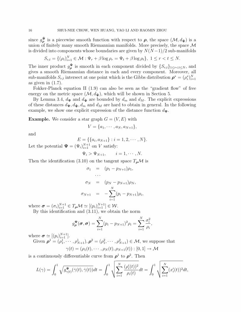
16 SHUI-NEE CHOW, WEN HUANG, YAO LI AND HAOMIN ZHOU
since gΨρ is a piecewise smooth function with respect to ρ, the space (M, dΨ) is a
union of finitely many smooth Riemannian manifolds. More precisely, the spaceMis divided into components whose boundaries are given by N(N−1)/2 sub-manifolds
Sr,t = {(ρi)Ni=1 ∈M : Ψr + β log ρr = Ψt + β log ρt}, 1 ≤ r < t ≤ N.
The inner product gΨρ is smooth in each component divided by {Sr,t}1≤r<t≤N , and
gives a smooth Riemannian distance in each and every component. Moreover, allsub-manifolds Sr,t intersect at one point which is the Gibbs distribution ρ∗ = (ρ∗i )
Ni=1
as given in (1.7).Fokker-Planck equation II (1.9) can also be seen as the “gradient flow” of free
energy on the metric space (M, dΨ), which will be shown in Section 5.By Lemma 3.4, dΨ and dΨ are bounded by dm and dM . The explicit expressions
of these distances dΨ, dΨ, dm and dM are hard to obtain in general. In the followingexample, we show one explicit expression of the distance function dΨ.
Example. We consider a star graph G = (V,E) with
V = {a1, · · · , aN , aN+1},and
E = {{ai, aN+1} : i = 1, 2, · · · , N}.Let the potential Ψ = (Ψi)
N+1i=1 on V satisfy:
Ψi > ΨN+1, i = 1, · · · , N.Then the identification (3.10) on the tangent space TρM is
σ1 = (p1 − pN+1)ρ1,
· · ·σN = (pN − pN+1)ρN ,
σN+1 = −N∑i=1
(pi − pN+1)ρi,
where σ = (σi)N+1i=1 ∈ TρM' [(pi)
N+1i=1 ] ∈ W .
By this identification and (3.11), we obtain the norm
gΨρ (σ,σ) =
N∑i=1
(pi − pN+1)2ρi =N∑i=1
σ2i
ρi,
where σ ' [(pi)N+1i=1 ].
Given ρ1 = (ρ11, · · · , ρ1
N+1),ρ2 = (ρ21, · · · , ρ2
N+1) ∈M, we suppose that
γ(t) = (ρ1(t), · · · , ρN(t), ρN+1(t)) : [0, 1]→Mis a continuously differentiable curve from ρ1 to ρ2. Then
L(γ) =
∫ 1
0
√gΨγ(t)(γ(t), γ(t))dt =
∫ 1
0
√√√√ N∑i=1
(ρ′i(t))2
ρi(t)dt =
∫ 1
0
√√√√ N∑i=1
(x′i(t))2dt,

FOKKER-PLANCK EQUATION ON THE GRAPHS 17
where we use the substitution xi(t) = 2√ρi(t) for i = 1, · · · , N . Let α(t) =
(x1(t), x2(t), · · · , xN(t)) for t ∈ [0, 1] and
D =
{(x1, x2, · · · , xN) ∈ RN :
N∑i=1
x2i < 4 and xi > 0 for i = 1, 2, · · · , N
}.
Then D is a convex subset of open ball with radius 2 in RN , and α is a continuouslydifferentiable curve in D from η1 = 2(
√ρ1
1, . . . ,√ρ1N) to η2 = 2(
√ρ2
1, . . . ,√ρ2N).
Clearly, we have
L(γ) =
∫ 1
0
√√√√ N∑i=1
(x′i(t))2dt ≥ ‖η1 − η2‖ = 2
√√√√ N∑i=1
(√ρ1i −
√ρ2i
)2
,
where ‖ · ‖ is the Euclidean norm.On the other hand, we take
α∗(t) = (x∗1(t), · · · , x∗N(t)) := tη1 + (1− t)η2
for t ∈ [0, 1]. In fact α∗ is the straight line segment in D from η1 to η2. Let
ρ∗i (t) = (x∗i (t))2/4 for i = 1, 2, · · · , N and ρ∗N+1(t) = 1− (
∑Ni=1 ρ
∗i (t)). Then
γ∗(t) = (ρ∗i (t))N+1i=1 : [0, 1]→M
is a continuously differentiable curve from ρ1 to ρ2. This implies that
L(γ∗) =
∫ 1
0
√√√√ N∑i=1
((x∗i (t))′)2dt = ‖η1 − η2‖ = 2
√√√√ N∑i=1
(√ρ1i −
√ρ2i
)2
.
Thus,
dΨ(ρ1,ρ2) = infγL(γ) = 2
√√√√ N∑i=1
(√ρ1i −
√ρ2i
)2
for ρ1 = (ρ11, · · · , ρ1
N+1),ρ2 = (ρ21, · · · , ρ2
N+1) ∈M. Finally, we note that the metric
dΨ can be extended naturally to the space M, i.e.,
dΨ(ρ1,ρ2) = 2
√√√√ N∑i=1
(√ρ1i −
√ρ2i
)2
for ρ1 = (ρ11, · · · , ρ1
N+1),ρ2 = (ρ21, · · · , ρ2
N+1) ∈M.
4. Fokker-Planck Equation I
In this section, we show that Fokker-Planck equation I (1.8) defined on a graphG = (V,E) with potentials Ψ = (Ψi)
Ni=1 on V and β ≥ 0 is the gradient flow of the
free energy F on the Riemannian manifold (M, dΨ) introduced in Section 3. Wealso show some basic properties of Fokker-Planck equation I (1.8).

18 SHUI-NEE CHOW, WEN HUANG, YAO LI AND HAOMIN ZHOU
Let β ≥ 0 be fixed and the free energy functional F be defined on the space M:
(4.1) F (ρ) =N∑i=1
Ψiρi + β
N∑i=1
ρi log ρi
where ρ = {ρi}Ni=1 ∈ M. Thus, we have the gradient flow of F on (M, gΨ) givenby,
(4.2)dρ
dt= −gradF (ρ),
where gradF (ρ) is in the tangent space TρM. We show that equation (4.2) is theFokker-Planck equation I (1.8) on M first.
If the differential of F , which is in the cotangent space, is denoted by diffF , then(4.2) could be expressed as
(4.3) gΨρ
(dρ
dt,σ
)= −diffF (ρ) · σ ∀σ ∈ TρM.
It is clear that
diffF ((ρi)Ni=1) = (Φi + β(1 + log ρi))
Ni=1(4.4)
for (ρi)Ni=1 ∈ M. By (4.3) and the identification (3.10), we are able to obtain the
explicit expression of the vector field on M.Now we are ready to show our first main result.
Theorem 4.1. Given a graph G = (V,E) with its vertex set V = {a1, a2, · · · , aN},edge set E, a potential Ψ = (Ψi)
Ni=1 on V and a constant β ≥ 0, let the neighborhood
set of a vertex ai be
N(i) = {j ∈ {1, 2, · · · , N}|{ai, aj} ∈ E},then
(1) The gradient flow of free energy F ,
F (ρ) =N∑i=1
Ψiρi + βN∑i=1
ρi log ρi
on the Riemannian manifold (M, dΨ) of probability densities ρ on V is
dρidt
=∑
j∈N(i),Ψj>Ψi
((Ψj + β log ρj)− (Ψi + β log ρi)) ρj
+∑
j∈N(i),Ψj<Ψi
((Ψj + β log ρj)− (Ψi + β log ρi)) ρi
+∑
j∈N(i),Ψj=Ψi
β(ρj − ρi)
for i = 1, 2, · · · , N , which is Fokker-Planck equation I (1.8).

FOKKER-PLANCK EQUATION ON THE GRAPHS 19
(2) For all β > 0, Gibbs distribution ρ∗ = (ρ∗i )Ni=1 given by
ρ∗i =1
Ke−Ψi/β with K =
N∑i=1
e−Ψi/β
is the unique stationary distribution of equation (1.8) in M. Furthermore,the free energy F attains its global minimum at Gibbs distribution.
(3) For all β > 0, there exists a unique solution
ρ(t) : [0,∞)→Mof equation (1.8) with initial value ρ0 ∈M, and ρ(t) satisfies:(a) the free energy F (ρ(t)) decreases as time t increases,(b) ρ(t)→ ρ∗ under the Euclidean metric of RN as t→ +∞.
As a direct consequence, we have the following result.
Corollary 4.2. Given the graph G = (V,E) with V = {a1, a2, · · · , aN} and potentialΨ = (Ψi)
Ni=1 on V , we have
(1) If the noise level β = 0, then Fokker-Planck equation I (1.8) for the discretestate space is
(4.5)dρidt
=∑
j∈N(i),Ψj>Ψi
(Ψj −Ψi)ρj +∑
j∈N(i),Ψj<Ψi
(Ψj −Ψi)ρi
for i = 1, 2, · · · , N .(2) In a special case when the potential is a constant at each vertice, this equation
is the master equation:
(4.6)dρidt
=∑j∈N(i)
β(ρj − ρi)
for i = 1, 2, · · · , N .
Remark 4.3. Given ρ0 ∈M and a continuous function
ρ(t) : [0, c)→Mfor some 0 < c ≤ +∞, we call such a function a generalized solution of equation (1.8)with initial value ρ0, if ρ(0) = ρ0 and ρ(t) ∈M satisfy equation (1.8) for t ∈ (0, c).In Appendix A, we give an example of a graph G and free energy to show that theremay not exist a generalized solution to (1.8) for some ρ0 ∈ ∂M :=M\M. We alsonote that the equation (1.8) is not well defined on the boundary ∂M :=M\M.
Remark 4.4. Equation (4.5) describes the time evolution of probability distributiondue to the potential energy and is also the probability distribution of a time ho-mogeneous Markov process on the graph G. The master equation is a first orderdifferential equation that describes the time evolution of the probability distribu-tion at every vertex in the discrete state space. Its entropy increases along with themaster equation. In this sense, Fokker-Planck equation I (1.8) is a generalization ofmaster equation. We refer to [5] for more details on the master equation.

20 SHUI-NEE CHOW, WEN HUANG, YAO LI AND HAOMIN ZHOU
Proof of Theorem 4.1. (1). We know that the gradient flow of free energy F on(M, dΨ) is given by equation (4.3),
gΨρ (dρ
dt,σ) = −diffF (ρ) · σ ∀σ ∈ TρM.
The left hand side of equation (4.3) is
(4.7) gΨρ (dρ
dt,σ) =
N∑i=1
dρidtpi
where σ = (σi)Ni=1 ' [(pi)
Ni=1]. By (4.4), the right hand side of equation (4.3) is
(4.8) −diffF (ρ) · σ = −N∑i=1
(Ψi + β(1 + log ρi))σi.
Using the identification (3.10), we have
N∑i=1
(Ψi + β(1 + log ρi))σi =N∑i=1
(Ψi + β log ρi)σi
=N∑i=1
(Ψi + β log ρi)(∑j∈N(i)
ΓΨij (ρ)(pi − pj))
=∑
{ai,aj}∈E,Ψi<Ψj
{(Ψi −Ψj) + β(log ρi − log ρj)}ρj(pi − pj)
+β∑
{ai,aj}∈E,Ψi=Ψj
(ρi − ρj)(pi − pj)
=N∑i=1
{ ∑j∈N(i),Ψj>Ψi
((Ψi −Ψj)ρj + β(log ρi − log ρj)ρj)
+∑
j∈N(i),Ψj<Ψi
((Ψi −Ψj)ρi + β(log ρi − log ρj)ρi)
+β∑
j∈N(i),Ψj=Ψi
(ρi − ρj)
}pi
Combining this equation with equations (4.3), (4.7) and (4.8), we have
N∑i=1
dρidtpi =
N∑i=1
{ ∑j∈N(i),Ψj>Ψi
((Ψj −Ψi)ρj + β(log ρj − log ρi)ρj)
+∑
j∈N(i),Ψj<Ψi
((Ψj −Ψi)ρi + β(log ρj − log ρi)ρi)
+β∑
j∈N(i),Ψj=Ψi
(ρj − ρi)
}pi.

FOKKER-PLANCK EQUATION ON THE GRAPHS 21
Since the above equality stands for any (pi)Ni=1 ∈ RN , we obtain Fokker-Flanck
equation I (1.8). This completes the proof of (1).
(2). It is well known that F attains its minimum at Gibbs density. By a directcomputation, we have that Gibbs distribution is a stationary solution. Let ρ =(ρi)
Ni=1 be a stationary solution of equation (1.8) inM. For σ = (σi)
Ni=1 ∈ TρM, we
let σ ' [(pi)Ni=1] for some (pi)
Ni=1 ∈ RN . Since ρ is the stationary solution, it implies
thatN∑i=1
(Ψi + β(1 + log ρi))σi
=N∑i=1
{ ∑j∈N(i),Ψj>Ψi
((Ψi −Ψj)ρj + β(log ρi − log ρj)ρj)
+∑
j∈N(i),Ψj<Ψi
((Ψi −Ψj)ρi + β(log ρi − log ρj)ρi)
+∑
j∈N(i),Ψj=Ψi
β(ρi − ρj)
}pi
= 0.
We note that for any (σi)N−1i=1 ∈ RN−1, if we take
σN = −N−1∑i=1
σi
then (σi)Ni=1 ∈ TρM. Thus one has
N−1∑i=1
{(Ψi + β(1 + log ρi))− (ΨN + β(1 + log ρN))}σi = 0
for any (σi)N−1i=1 ∈ RN−1. This implies
(Ψi + β log ρi)− (ΨN + β log ρN) = 0,
which is
ρi = eΨN−Ψi
β ρNfor i = 1, 2, · · · , N − 1.
Combining this fact with∑N
i=1 ρi = 1, we have ρi = 1Ke−Ψi/β = ρ∗i for i =
1, 2, · · · , N , where K =∑N
i=1 e−Ψi
β . This completes the proof of (2).
(3). Let a continuous function
ρ(t) : [0, c)→Mfor some 0 < c ≤ +∞ be a solution of equation (1.8) with initial value ρ0 ∈ M.For any ρ0 ∈ M, there exists a maximal interval of existence [0, c(ρ0)) and 0 <
22 SHUI-NEE CHOW, WEN HUANG, YAO LI AND HAOMIN ZHOU
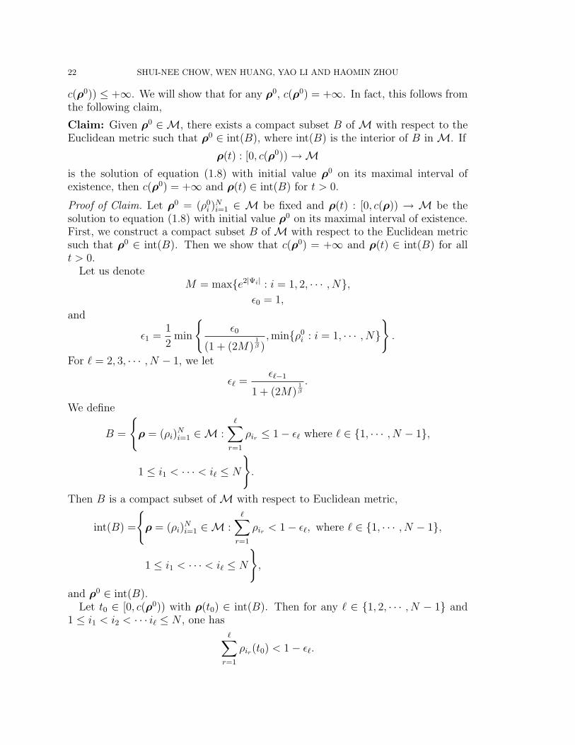
c(ρ0)) ≤ +∞. We will show that for any ρ0, c(ρ0) = +∞. In fact, this follows fromthe following claim,
Claim: Given ρ0 ∈ M, there exists a compact subset B of M with respect to theEuclidean metric such that ρ0 ∈ int(B), where int(B) is the interior of B in M. If
ρ(t) : [0, c(ρ0))→Mis the solution of equation (1.8) with initial value ρ0 on its maximal interval ofexistence, then c(ρ0) = +∞ and ρ(t) ∈ int(B) for t > 0.
Proof of Claim. Let ρ0 = (ρ0i )Ni=1 ∈ M be fixed and ρ(t) : [0, c(ρ)) → M be the
solution to equation (1.8) with initial value ρ0 on its maximal interval of existence.First, we construct a compact subset B of M with respect to the Euclidean metricsuch that ρ0 ∈ int(B). Then we show that c(ρ0) = +∞ and ρ(t) ∈ int(B) for allt > 0.
Let us denoteM = max{e2|Ψi| : i = 1, 2, · · · , N},
ε0 = 1,
and
ε1 =1
2min
{ε0
(1 + (2M)1β ),min{ρ0
i : i = 1, · · · , N}
}.
For ` = 2, 3, · · · , N − 1, we let
ε` =ε`−1
1 + (2M)1β
.
We define
B =
{ρ = (ρi)
Ni=1 ∈M :
∑r=1
ρir ≤ 1− ε` where ` ∈ {1, · · · , N − 1},
1 ≤ i1 < · · · < i` ≤ N
}.
Then B is a compact subset of M with respect to Euclidean metric,
int(B) =
{ρ = (ρi)
Ni=1 ∈M :
∑r=1
ρir < 1− ε`, where ` ∈ {1, · · · , N − 1},
1 ≤ i1 < · · · < i` ≤ N
},
and ρ0 ∈ int(B).Let t0 ∈ [0, c(ρ0)) with ρ(t0) ∈ int(B). Then for any ` ∈ {1, 2, · · · , N − 1} and
1 ≤ i1 < i2 < · · · i` ≤ N , one has∑r=1
ρir(t0) < 1− ε`.

FOKKER-PLANCK EQUATION ON THE GRAPHS 23
Moreover ∑r=1
ρir(t) < 1− ε`
for small enough t > t0 by continuity. Thus ρ(t) ∈ int(B) for small enough t > t0.With the above discussion and the compactness of B, we are ready to prove that
c(ρ0) = +∞. To show this, it is sufficient to prove that ρ(t) ∈ int(B) for all t > 0.Let us assume this is not true, which means the solution ρ(t) hits the boundary. Inthis case, there exists t1 > 0 such that ρ(t1) ∈ ∂B and ρ(t) ∈ int(B) for all t ∈ [0, t1).Since ρ(t1) ∈ ∂B, we can find 1 ≤ i1 < · · · < il ≤ N such that 1 ≤ l ≤ N − 1 and
(4.9)l∑
r=1
ρir(t1) = 1− εl.
Let A = {i1, i2, · · · , i`} and Ac = {1, 2, · · · , N} \ A. Then for any j ∈ Ac,
(4.10) ρj(t1) ≤ 1−
(∑r=1
ρir(t1)
)= ε`.
Since ρ(t1) ∈ B, we have`−1∑j=1
ρsj(t1) ≤ 1− ε`−1,
for any 1 ≤ s1 < s2 < · · · < s`−1 ≤ N . Hence for each i ∈ A,
(4.11) ρi(t1) ≥ 1− ε` − (1− ε`−1) = ε`−1 − ε`.Combining equations (4.10), (4.11) and the fact
ε` ≤ε`−1
1 + (2M)1β
,
one has, for any i ∈ A, j ∈ Ac,(4.12) Ψj −Ψi + β(log ρj − log ρi) ≤ Ψj −Ψi + β(log ε` − log(ε`−1 − ε`)) ≤ − log 2.
Since the graph G is connected, there exists i∗ ∈ A, j∗ ∈ Ac such that {ai∗ , aj∗} ∈ E.Thus
(4.13)∑
i∈A,j∈Ac,{ai,aj}∈E
ΓΨij (ρ(t1)) ≥ ΓΨ
i∗j∗(ρ(t1)) > 0.

24 SHUI-NEE CHOW, WEN HUANG, YAO LI AND HAOMIN ZHOU
Now by (4.12) and (4.13), one has
d
dt
∑r=1
ρir(t) |t=t1 =∑i∈A
∑j∈N(i)
ΓΨij (ρ(t1)) (Ψj −Ψi + β(log ρj(t1)− log ρi(t1)))
=∑i∈A
{∑
j∈A∩N(i)
ΓΨij (ρ(t1)) (Ψj −Ψi + β(log ρj(t1)− log ρi(t1)))
+∑
j∈Ac∩N(i)
ΓΨij (ρ(t1)) (Ψj −Ψi + β(log ρj(t1)− log ρi(t1)))}
=∑i∈A
∑j∈Ac∩N(i)
ΓΨij (ρ(t1)) (Ψj −Ψi + β(log ρj(t1)− log ρi(t1)))
≤ − log 2∑i∈A
∑j∈Ac∩N(i)
ΓΨij (ρ(t1))
= − log 2∑
i∈A,j∈Ac,{ai,aj}∈E
ΓΨij (ρ(t1))
≤ − log 2ΓΨi∗j∗(ρ(t1)) < 0.
Combining this with (4.9), it is clear that
l∑i=1
ρir(t1 − δ) > 1− εl
for sufficiently small δ > 0. This implies ρ(t1 − δ) /∈ B , and it contradicts the factthat ρ(t) ∈ int(B) for t ∈ [0, t1). This completes the proof of the Claim. �
Given ρ0 ∈M, by the above Claim, there exists a unique solution
ρ(t) : [0,∞)→Mto equation (1.8) with initial value ρ0, and we can find a compact subset B ofM withrespect to Euclidean metric such that {ρ(t) : t ∈ [0,+∞)} ⊂ B. For t ∈ (0,+∞),
dF (ρ(t))
dt= diffF (ρ(t)) · dρ
dt(t) = −gΨ
ρ(t)(dρ
dt(t),
dρ
dt(t)) ≤ 0
and thusdF (ρ(t))
dt= 0 if and only if
dρ(t)
dt= 0.
This is equivalent to ρ(t) = (ρ∗i )Ni=1 by (2). This implies that the free energy F (ρ(t))
decreases as time t increases.Finally, we show that ρ(t) → ρ∗ under the Euclidean metric of RN as t → +∞.
We let
ω(ρ0) =
{ρ ∈ RN : ∃ ti → +∞ such that lim
i→+∞ρ(ti) = ρ in Euclidean metric
}be the ω-limit set of ρ0. Clearly, ω(ρ0) ⊂ B is a compact set of RN with respect toEuclidean metric.

FOKKER-PLANCK EQUATION ON THE GRAPHS 25
To show ρ(t)→ ρ∗ under the Euclidean metric of RN when t→ +∞, it is sufficientto show that ω(ρ0) = {ρ∗}. Since ω(ρ0) is a compact set and the free energy F is con-tinuous on M, we can find ρ1 ∈ ω(ρ0) such that F (ρ1) = max{F (ρ) : ρ ∈ ω(ρ0)}.Then there exists ti → +∞ such that limi→+∞ ρ(ti) = ρ1 and limi→+∞ ρ(ti−1) = ρ2
for some ρ2 ∈M. If we let ρ2(t) be the solution to equation (1.8) with initial valueρ2, then ρ2(0) = ρ2 and ρ2(1) = ρ1. Note that
dF (ρ2(t))
dt= diffF (ρ2(t)) · dρ
2
dt(t) = −gΨ
ρ2(t)(dρ2
dt(t),
dρ2
dt(t)) ≤ 0
and thusdF (ρ2(t))
dt= 0 if and only if
dρ2(t)
dt= 0,
which is equivalent to ρ2(t) = ρ∗ by (2). Hence if ρ1 6= ρ∗, then F (ρ2) > F (ρ1),which is a contradiction with F (ρ1) = max{F (ρ) : ρ ∈ ω(ρ0)}. So we must haveρ1 = ρ∗. Thus,
max{F (ρ) : ρ ∈ ω(ρ0)} = F (ρ∗).
It is well known that ρ∗ is the unique minimal value point of F . This impliesω(ρ0) = {ρ∗}. This completes the proof of (3). �
There are many reasons why we consider Fokker-Planck equation I (1.8) on themanifoldM instead of its closure. One of the main reasons is thatM is a manifoldwith boundary and its tangent space is only well defined in its interior. Anotherreason is that the free energy is not differentiable when ρi = 0 for some i. Andit is also not clear how the Riemannian metric dΨ on M can be extended to M.Moreover, even if the distance is well defined on M, there may not be a solutionto the equation (1.8) with initial value on the boundary ∂M (see the example inAppendix A).
Theorem 4.1 (3) guarantees the solution of (1.8) can never attain the boundary∂M if the initial value is in M. In practice, we still need an equation to describethe transient process if the initial value is on the boundary. However, we think thatthe study of this important aspect is already beyond the scope of this paper. Thediscussion on it will be given in a sequel paper.
5. Fokker-Planck Equation II
Given a graph G = (V,E), we consider a time homogeneous Markov process X(t),on the set V . We assume that X(t) is generated by a potential function Ψ = (Ψi)
Ni=1
on V as a “gradient flow”. If the process starts at a vertex ai at time t, then thetransition probability to the vertex aj at time t+ h is given by
Pr(X(t+ h) = aj|X(t) = ai)
=
(Ψi −Ψj)h+ o(h) if j ∈ N(i),Ψj < Ψi,
1−∑
k∈N(i),Ψk<Ψi
(Ψi −Ψk)h+ o(h) if j = i,
0 otherwise,
where o(h)/|h| → 0 as h→ 0.

26 SHUI-NEE CHOW, WEN HUANG, YAO LI AND HAOMIN ZHOU
The generating matrix Q = [Qij]N×N for the Markov process can be defined by
Qij =
{Ψi −Ψj if {ai, aj} ∈ E,Ψj < Ψi,
0 otherwise,
which is the transition rate from i to j, and Qii = −∑
j 6=iQij.
Let ρ(t) = (ρi(t))Ni=1, where ρi(t) = Pr(X(t) = ai) for i = 1, 2, · · · , N . The time
evolution of probability distribution ρ(t) is given by a forward Kolmogorov equation:{∂ρ∂t
(t) = ρ(t)Q
ρ(0) = {ρ0i }Ni=1,
or in an explicit form,
(5.1)dρidt
=∑
j∈N(i),Ψj>Ψi
(Ψj −Ψi)ρj +∑
j∈N(i),Ψj<Ψi
(Ψj −Ψi)ρi
for i = 1, 2, · · · , N .We can consider X(t) as an analog of the following gradient flow in Euclidean
space :
(5.2)dx
dt= −∇Ψ(x), x ∈ RN
and the forward Kolmogorov equation (5.1) is an analog of the corresponding de-generate Fokker-Planck equation without noise,
(5.3)∂ρ
∂t= ∇ · (∇Ψρ).
For this reason, we call the Markov process X(t) the gradient Markov process gen-erated by discrete potential function Ψ on the graph G. Equation (5.1) can also beconsidered as a discretization of equation (5.3) with an upwind scheme [29].
An important observation is that in the continuous state space RN , Fokker-Planckequation (1.2) can be obtained by adding “white noise” to the degenerate Fokker-Planck equation (5.3). As an analog, we will obtain the Fokker-Planck equation ona discrete space by adding “white noise” with strength
√2β to equation (5.1).
Suppose we rewrite Fokker-Planck equation (1.2) in the following degenerate fash-ion:
ρt = ∇ · (∇Ψρ) + β∆ρ = ∇ · [∇(Ψ + β log ρ)ρ],
and its corresponding free energy in the following:
F =
∫RN
(Ψ + β log ρ)ρdx.
This indicates that if white noise√
2βdWt is added to system (5.2) on RN , it isequivalent to consider a new potential
Ψ(x, t) = Ψ(x) + β log ρ(x, t)
in the gradient flow (5.3).

FOKKER-PLANCK EQUATION ON THE GRAPHS 27
Remark 5.1. This new potential function Ψ +β log ρ(x, t) is called Onsager’s poten-tial, and its derivative is called Onsager thermodynamic flux [7, 39].
As an analog, adding “white noise” to a time homogeneous Markov process X(t)on a graph is equivalent to “changing the potential” to a new potential defined by:
Ψi(t) = Ψi + β log ρi(t)
for i = 1, 2, · · · , N . For this modified potential Ψ, we have a new Markov processXβ(t) which is time inhomogeneous, and may be considered as a “white noise”perturbation from the original homogeneous Markov process X(t). More precisely,the conditional distribution of aj at time t+ h given ai at time t is given by
Pr(Xβ(t+ h) = aj|Xβ(t) = ai)
=
(Ψi(t)− Ψj(t))h+ o(h), if j ∈ N(i), Ψj(t) < Ψi(t),
1−∑
k∈N(i),Ψk(t)<Ψi(t)
(Ψi(t)− Ψk(t))h+ o(h) if j = i,
0, otherwise.
The time evolution of probability distribution (ρi(t))Ni=1 of Xβ(t) satisfies the follow-
ing forward Kolmogorov equation:
dρidt
=∑
j∈N(i),Ψj>Ψi
((Ψj + β log ρj)− (Ψi + β log ρi))ρj
+∑
j∈N(i),Ψj<Ψi
((Ψj + β log ρj)− (Ψi + β log ρi))ρi,
which is exactly Fokker-Planck equation II (1.9). On the other hand, we can alsoconsider Fokker-Planck equation II (1.9) as a gradient flow of the free energy on thespace M with an appropriate inner product. Let us define the inner product gΨ
ρ
based on the new potential Ψi(t), and use it to induce a distance dΨ as shown inSection 3. The free energy F on the space M is given by:
F (ρ) =N∑i=1
Ψiρi + βN∑i=1
ρi log ρi
where ρ = (ρi)Ni=1 ∈M.
Since ρ ∈ M 7→ gΨρ may not be continuous, there may not exist a gradient
flow of F on (M, dΨ). However, we can consider a generalized gradient flow of Fon (M, dΨ) because of the special relationship between M and its tangent spaces.
More precisely, the derivative dρ(t)dt∈ Tρ(t)M is the same as the one computed using
Euclidean metric. Thus, we can consider the following equation as our generalizedgradient flow:
(5.4) gΨρ (dρ
dt(t),σ) = −diffF (ρ(t)) · σ ∀σ ∈ TρM,

28 SHUI-NEE CHOW, WEN HUANG, YAO LI AND HAOMIN ZHOU
where diffF is the differential of F (see (4.4)). This also implies:
dF (ρ(t))
dt= diffF (ρ(t)) · dρ(t)
dt= −gΨ
ρ(t)
(dρ(t)
dt,dρ(t)
dt
).(5.5)
We have the following theorem:
Theorem 5.2. Given the graph G = (V,E) with V = {a1, a2, · · · , aN}, potentialΨ = (Ψi)
Ni=1 on V and β ≥ 0, we consider the gradient Markov process X(t) gener-
ated by the potential Ψ. Then we have
(1) Fokker-Planck equation II (1.9)
dρidt
=∑
j∈N(i),Ψj>Ψi
((Ψj + β log ρj)− (Ψi + β log ρi))ρj
+∑
j∈N(i),Ψj<Ψi
((Ψj + β log ρj)− (Ψi + β log ρi))ρi
describes the time evolution of probability distribution of Xβ(t), where Xβ(t)is the time inhomogeneous Markov process perturbed by “white noise” fromthe original Markov process X(t).
(2) Fokker-Planck equation II (1.9) is the generalized gradient flow (5.4) of thefree energy F on the metric space (M, dΨ) of probability densities ρ on V .
(3) For all β > 0, Gibbs distribution ρ∗ = (ρ∗i )Ni=1
ρ∗i =1
Ke−Ψi/β with K =
N∑i=1
e−Ψi/β
is the unique stationary distribution of equation (1.9) in M, and the freeenergy F attains minimum at Gibbs distribution.
(4) For all β > 0, there exists a unique solution ρ(t) : [0,∞) →M to equation(1.9) with initial value ρ0 ∈M, and ρ(t) satisfies(a) The free energy F (ρ(t)) decreases when time t increases.(b) ρ(t)→ ρ∗ under the Euclid metric of RN when t→ +∞.
Proof. (1). Result in (1) comes from the discussion in the beginning of this section.(2). A continuously differentiable function ρ(t) : [0, c) → M for some c > 0 or
c = +∞ is called a solution of equation (1.9) with initial value ρ ∈ M, if ρ(0) = ρand ρ(t) satisfies equation (1.9) for t ∈ [0, c). Since the Fokker-Planck equation II(1.9) is Lipschitz continuous, by the existence and uniqueness theorem of ordinarydifferential equations, it is clear that for any ρ ∈M, there exists a maximal interval[0, c(ρ)) in which the solution to equation (1.9) with initial value ρ is uniquelydefined with c(ρ) > 0 or c(ρ) = +∞.

FOKKER-PLANCK EQUATION ON THE GRAPHS 29
Let ρ(t) : [0, c) →M be a solution of (1.9). For σ = (σi)Ni=1 ∈ Tρ(t)M, we take
(pi)Ni=1 ∈ RN such that σ ' [(pi)
Ni=1]. Then by (4.4), we have
N∑i=1
(Ψi + β(1 + log ρi))σi =N∑i=1
(Ψi + β log ρi)σi(5.6)
=N∑i=1
(Ψi + β log ρi)
∑j∈N(i)
ΓΨij (ρ)
(pi − pj)
=∑
{ai,aj}∈E,Ψi<Ψj
{(Ψi −Ψj) + β(log ρi − log ρj)}ρj(pi − pj)
+ β∑
{ai,aj}∈E,Ψi=Ψj
(Ψi − Ψj)(pi − pj)
=∑i
{ ∑j∈N(i),Ψj>Ψi
((Ψi −Ψj)ρj + β(log ρi − log ρj)ρj)
+∑
j∈N(i),Ψj<Ψi
((Ψi −Ψj)ρi + β(log ρi − log ρj)ρi)
}pi.
Combining this equation with Fokker-Planck equation II (1.9), and by identifications(3.12) and (3.14), we have
diffF (ρ(t)) · σ =N∑i=1
(Ψi + β(1 + log ρi))σi
=N∑i=1
{ ∑j∈N(i),Ψj>Ψi
((Ψi −Ψj)ρj + β(log ρi − log ρj)ρj)
+∑
j∈N(i),Ψj<Ψi
((Ψi −Ψj)ρi + β(log ρi − log ρj)ρi)
}pi
= −N∑i=1
dρidtpi = −gΨ
ρ(t)
(dρ(t)
dt,σ
).
Hence (5.4) is true, and this finishes the proof of (2).
(3). Using (5.6) and replacing identification (3.10) by identification (3.12), theproof of (3) is completely similar to the proof of (2) in Theorem 4.1.
(4). Using (5.5) and replacing ΓΨij (ρ) by ΓΨ
ij (ρ) in the proof of (3) in Theorem4.1, we get the proof of (4) in a similar way. �
Remark 5.3. We note that Fokker-Planck equation I and Fokker-Planck equationII are very different even though they differ only by one term. In fact, Fokker-Planck equation II is not a gradient flow of the free energy on a smooth Riemannianmanifold of the probability space, but it is a gradient flow if we allow the Riemannian

30 SHUI-NEE CHOW, WEN HUANG, YAO LI AND HAOMIN ZHOU
manifold of probability space to be piecewise smooth. More importantly, Fokker-Planck equation II is based on two important concepts, white noise and ”nonlinear”Laplace operator for Markov processes on graphs.
Remark 5.4. In the above discussion, a time-homogeneous Markov process is given asthe gradient Markov process generated by a potential Ψ on a graph G = (V,E). Onthe other hand, if the potential is not given but a time-homogeneous Markov processis given, then we may reconstruct its potential function under some conditions. LetG be a weighted directed simple graph without self-loop or multi-edge. Supposewe have a time-homogeneous Markov process on G, the Markov process is calledgradient like If every directed loop from ai to itself has zero total weight. In thiscase, a potential energy function can be defined on this graph, and it is unique upto a constant. To better illustrate it, we use the following example.
Example. We consider a graph G = (V,E) with a time-homogeneous Markovprocess as shown in Figure 2, which is directed and weighted. In this graph,V = {a1, a2, a3, a4, a5} and the number on each directed edge is the transition rate.Since the underlying weighted directed graph is gradient like, we may associate thepotential energy on each vertex as in Figure 3. With this potential function, we canfind its free energy and the Fokker-Planck equation.
Figure 2. “gradient like”transition graph
Figure 3. associated po-tential function
The transition probability rate matrix Q of this Markov process induced by Figure2 is:
Q =
0 1 0 0 00 0 0 0 00 2 0 0 10 0 1 0 20 1 0 0 0
6. Connections to Upwind Schemes
From discussions in previous sections, it is clear that Fokker-Planck equations(1.8) and (1.9) on a graph are not typical discretizations of the Fokker-Planckequation in continuous state space. Moreover, one cannot obtain a Fokker-Planckequation in discrete state space with desired properties by simply discretizing the

FOKKER-PLANCK EQUATION ON THE GRAPHS 31
Fokker-Planck equation in continuous state space with commonly used finite differ-ence schemes. However, it is worth mentioning that Fokker-Planck equations (1.8)and (1.9) are motivated by the well-known strategies in finite difference methods,namely the upwind schemes for hyperbolic equations. In this section, we explainthese connections in detail, and show that our discrete Fokker-Planck equations areactually consistent to the Fokker-Planck equation in continuous state space, pro-vided that the discrete spaces are discretizations of the continuous state space.
For simplicity, let us demonstrate the connections on a 1-D lattice G = (V,E) withvertex set V = {a1, · · · , aN} (N ≥ 3) and E = {{ai, ai+1} : i = 1, 2, · · · , N − 1}.We view the lattice as equal partition points of the interval [0, 1] with mesh sizeh. We also assume that the potential function on V does not have equal valueson adjacent points. Then our discrete Fokker-Planck equation I at vertex ai, i ∈{2, 3, · · · , N − 1}, is given by,
dρidt
= ((Ψi+1 −Ψi)ρi+1 − (Ψi −Ψi−1)ρi)
+β((log ρi+1 − log ρi)ρi+1 − (log ρi − log ρi−1)ρi)
if Ψi+1 > Ψi > Ψi−1,
dρidt
= ((Ψi+1 −Ψi)ρi − (Ψi −Ψi−1)ρi−1)
+β((log ρi+1 − log ρi)ρi − (log ρi − log ρi−1)ρi−1)
if Ψi+1 < Ψi < Ψi−1,
dρidt
= ((Ψi+1 −Ψi)ρi+1 − (Ψi −Ψi−1)ρi−1)
+β((log ρi+1 − log ρi)ρi+1 − (log ρi − log ρi−1)ρi−1)
if Ψi+1 > Ψi,Ψi−1 > Ψi,
dρidt
= ((Ψi+1 −Ψi)ρi − (Ψi −Ψi−1)ρi)
+β((log ρi+1 − log ρi)ρi − (log ρi − log ρi−1)ρi)
if Ψi+1 < Ψi,Ψi−1 < Ψi.
First, we consider the drift terms, i.e., the ones involving the potentials, on theright hand side of the equations. It is obvious that when the potential is increasingat vertex ai, which corresponds to the first scenario as Ψi+1 > Ψi > Ψi−1, the term(Ψi+1 −Ψi)ρi+1 − (Ψi −Ψi−1)ρi involves density values ρi+1 and ρi, which are fromthe right side of position i. If one views the differences in potentials (Ψi−Ψi−1) and(Ψi+1−Ψi), which are all positive, as the convection coefficient, then it indicates thatthe characteristic line goes from right to the left. In other words, in this situation theinformation propagates to the left, which is like “wind blowing” to the left direction.Thus the right hand side of the equation only involves information from the upwind(higher potential in this case) direction. Similarly, the upwind direction for thedecreasing potential case with Ψi+1 < Ψi < Ψi−1 is from the left to the right. Andthe Fokker-Planck equation only relies on the values ρi and ρi−1, which is from its

32 SHUI-NEE CHOW, WEN HUANG, YAO LI AND HAOMIN ZHOU
upwind direction. In the other two cases, there are no clear upwind directions andtherefore central differences are used. Moreover, one can see that the evolution ofρi only depends on its neighboring values with higher potentials. And this is alsotrue for general graphs.
The appearance of upwind directions in Fokker-Planck equations I and II becomesnatural if we take a closer look at the working mechanism of the drift terms. If weignore the diffusion terms by taking β = 0, then the probability density ρi evolvesaccording to the gradient descent direction. The consequence is that the probabilityis clustered on local minima of the potentials. And therefore, their correspondingdensity functions are combinations of Dirac Delta functions sitting on the minima.This is very similar to the shock (discontinuities in solutions) formation in nonlinearhyperbolic conservation laws, in which upwind idea is considered as a fundamentalstrategy in designing shock capturing schemes. On the other hand, if one uses centraldifferences in shock formation, numerical oscillations, which are called Gibbs’ phe-nomenon, are inevitable. For more discussions on numerical schemes for nonlinearconservation laws, readers are referred to books such as [6, 29].
7. The Parrondo’s Paradox
It is known in game theory that it is possible to construct a winning strategyby playing two losing strategies alternately. This is often referred as Parrondo’sparadox [1, 22, 23, 24, 38, 40, 41]. In this section, we explain, by using a discreteFokker-Planch equation, the paradox of free energy for the flashing ratchet model[3, 1, 24, 40, 41] on a simple graph.
We consider a graph G = (V,E) having 23 vertices:
V = {a1, a2, · · · , a23} and E = {{ai, ai+1} : i = 1, · · · , 22},with two different potential functions ΨA and ΨB given on the graph. ΨA is definedas shown in Figure 4 and ΨB
i = 0 for i = 1, 2, · · · , 23. The values of ΨA are listedin Table 1,
Table 1. Potential function ΨA
ai 1 2 3 4 5 6 7 8 9 10 11 12ΨAi 5 3.4 2.2 2.5 2.8 3.1 1.9 2.2 2.5 2.8 1.6 1.9
ai 13 14 15 16 17 18 19 20 21 22 23ΨAi 2.2 2.5 1.3 1.6 1.9 2.2 1 1.3 1.6 1.9 4
Here we fix the temperature β = 0.05. For any probability density ρ = (ρi)23i=1 on
V , we consider two free energy functionals:
FA(ρ) =23∑i=1
ΨAi ρi + 0.05
23∑i=1
ρi log ρi
FB(ρ) =23∑i=1
ΨBi ρi + 0.05
23∑i=1
ρi log ρi = 0.0523∑i=1
ρi log ρi.

FOKKER-PLANCK EQUATION ON THE GRAPHS 33
Figure 4. Potential function ΨA.
Free energy FA(ρ) induces a Markov process called Process A. Using Theorem 4.1(1) with ΨA, we obtain a discrete Fokker-Planck equation, denoted as Equation Afor Process A. (Here we omit the detailed expression of Equation A for simplicity.)Similarly, free energy FB(ρ) induces another Markov process called Process B, andits Fokker-Planck equation is given by
dρ1
dt= 0.05(ρ2 − ρ1)
dρidt
= 0.05(ρi+1 + ρi−1 − 2ρi), 1 < i < 23
dρ23
dt= 0.05(ρ22 − ρ23)
.
We call it Equation B.By Theorem 4.1 (3), free energy functionals FA and FB decrease monotonically
along the solutions of Equations A and B respectively as time increases. Both pro-cesses are energy dissipative. However, if we apply processes A and B alternatingly,which is the classical flashing ratchet model, then we will observe an energy gainingprocess. In another word, in this view point, the flashing ratchet is also a Parrondo’sparadox of free energy.
Figure 5. Initial Distribution Figure 6. Final distribution

34 SHUI-NEE CHOW, WEN HUANG, YAO LI AND HAOMIN ZHOU
More precisely, we choose an initial distribution ρ0 as shown in Figure 5. The peakof ρ0 is on the right. We choose time interval length T = 0.3 and we use Equation Awhen 0 ≤ t < T , and Equation B when T ≤ t < 2T . Then we repeat the processes.After taking ABABAB · · · for 400-times, the peak of probability distribution movedto the left hand side (Figure 6). This indicates a directed motion from the lowerpotential places to higher potential regions. This can be used to explain the directedmotions by molecular motors.
Figure 7. First 10 process
Figure 8. The free energy at the end of Process A for the first 400 iterations
To better illustrate this process, we show the free energy changes in Figures 7and 8. Figure 7 shows the free energy in the first 10 iterations. Process A ends attime T , and Process B begins. At time 2T , Process B ends, and another Process Astarts. These steps are repeated. Although the free energy functionals decrease on

FOKKER-PLANCK EQUATION ON THE GRAPHS 35
each process A and B, the free energy function FA(ρ) at time 3T is still higher thanthat at time T . So applying the two processes A and B alternatingly, we observean energy gaining process at the end of process A, i.e., at times T , 3T , 5T, · · · .We show this energy gaining phenomenon in Figure 8. For a similar example in acontinuous state space, see [11].
Appendix A. A counterexample
Applying Theorem 4.1 (1) to a graph G with Ψ and β > 0, we obtain Fokker-Planck equation (1.8) on M. For ρ0 ∈ M, a continuous function ρ(t) : [0, c)→Mfor some c > 0 or c = +∞ is defined to be a solution of equation (1.8) with initialvalue ρ0 if ρ(0) = ρ0 and ρ(t) ∈ M satisfies equation (1.8) for t ∈ (0, c). Inthe following. we present an example for which there does not exist a solution ofequation (1.8) for an initial value ρ0 ∈ ∂M :=M\M.
Example. We consider a graph with 3 vertices:
V = {a1, a2, a3} and E = {{a1, a3}, {a2, a3}}.In this case, we have
M = {ρ = (ρi)3i=1 ∈ R3 : ρ1 + ρ2 + ρ3 = 1 and ρi > 0 for i = 1, 2, 3}
and
M = {ρ = (ρi)3i=1 ∈ R3 : ρ1 + ρ2 + ρ3 = 1 and ρi ≥ 0 for i = 1, 2, 3}.
We assign potential Ψ = (Ψi)3i=1 on V with Ψ1 > Ψ3 and Ψ2 > Ψ3, and fix β > 0.
Applying Theorem 4.1 (1) for G, Ψi and β, we obtain Fokker-Planck equation I (1.8)on M as follow:
(A.1)
dρ1
dt= (Ψ3 −Ψ1 + β(log ρ3 − log ρ1)) ρ1
dρ2
dt= (Ψ3 −Ψ2 + β(log ρ3 − log ρ2)) ρ2
dρ3
dt=
2∑i=1
(Ψi −Ψ3 + β(log ρi − log ρ3)) ρi
Now let ρ0 = (0, 1, 0) ∈ ∂M. Then we claim that there is no solution to equation(A.1) with initial value ρ0.
In fact, if the claim is not true, then there exists a continuous function
ρ(t) = (ρ1(t), ρ2(t), ρ3(t)) : [0, c)→Mfor some c > 0 or c = +∞ such that ρ(0) = ρ0 and ρ(t) ∈ M satisfying equation(A.1) for t ∈ (0, c). By (A.1), one has
d log ρ1(t)
dt= (Ψ3 −Ψ1) + β(log ρ3(t)− log ρ1(t))
d log ρ2(t)
dt= (Ψ3 −Ψ2) + β(log ρ3(t)− log ρ2(t))
36 SHUI-NEE CHOW, WEN HUANG, YAO LI AND HAOMIN ZHOU
for t ∈ (0, c). Let x(t) = log ρ1(t)− log ρ2(t) for t ∈ (0, c), then one gets
dx(t)
dt= Ψ2 −Ψ1 − βx(t)
for t ∈ (0, c). Fix T ∈ (0, c). It is clear that for any 0 < s < T ,
(A.2) eβTx(T ) = eβsx(s) +
∫ T
s
e(Ψ2−Ψ1)tdt.
Since lims↘0 eβsx(s) = −∞ and lims↘0
∫ Tse(Ψ2−Ψ1)tdt =
∫ T0e(Ψ2−Ψ1)tdt, if one lets
s ↘ 0 in (A.2), then one has eβTx(T ) = −∞, i.e., ρ1(T ) = −∞. This is a contra-diction to (ρ1(T ), ρ2(T ), ρ3(T )) ∈M.
References
[1] Ait-Haddou, R. and Herzog, W., Brownian Ratchet Models of Molecular Motors, Cell Bio-chemistry and Biophysics 38 (2) (2003) 191-213.
[2] Ambrosio, L., Gigli, N. and Savare, G., Gradient Flows: In Metric Spaces and in the Space ofProbability Measures, Lectures in Mathematics ETH Zurich Birkhauser Verlag, Basel, 2008.
[3] Astumian, RD., Thermodynamics and kinetics of a Brownian motor, Science 276(1997) 917-922.
[4] Bonciocat, A. I. and Sturm, K. -T., Mass transportation and rough curvature bounds fordiscrete spaces, J. Funct. Anal. 256 (9) (2009) 2944-2966.
[5] Van den Broeck, C., The master equation and some applications in physics, Stochastic pro-cesses applied to physics, World Sci. Publishing, Singapore, 1985, 1-28.
[6] Buet, C. and Cordier, S., Numerical Analysis of Conservative and Entropy Schemes for theFokker-Planck-Landau Equation, SIAM J. Numer. Anal. 36 (3) (1999) 953-973.
[7] Bergmann, P. G. and Lebowitz, J. L., New Approach to Nonequilibrium Processes, Phys.Rev. 99 (2) (1955) 578-587.
[8] Carlen, E. A. and Gangbo, W., Constrained steepest descent in the 2-Wasserstein metric,Ann. of Math. (2) 157 (3) (2003) 807-846.
[9] Carlen, E. A. and Gangbo, W., On the solution of a model Boltzmann equation via con-strained steepest ascent in a Wasserstein metric, Arch. Rational Mech. Ana. 172 (1) (2004)21-64.
[10] Cordero, D., Gangbo, W. and Houdre, C., Inequalities for generalized entropy and optimaltransportation. Comteporary Mathematics, AMS Vol 353, 2004.
[11] Chow, S.-N., Huang, W., Li, Y. and Zhou, H. M., A free energy based mathematical studyfor molecular motors, Regular and Chaotic Dynamics 16 (2011) 117-127.
[12] Cordero-Erausquin, D., McCann, R. J. and Schmuckenschlager, M., A Riemannian interpo-lation inequality a la Borell, Brascamp and Lieb., Invent. Math. 146 (2) (2001) 219-257.
[13] Dobrushin, R. L., Prescribing a system of random variables by conditional distributions,Theor. Probab. Appl. 15 (1970) 458-486.
[14] Dolbeault, J., Kinderlehrer, D. and Kowalczyk, M., Remarks about the flashing rachet,Partial differential equations and inverse problems, Contemp. Math. Vol. 362, Amer. Math.Soc., 2004, 167-175.
[15] Ellis, R. S., Entropy, Large Deviations and Statistical Mechanics, Grundlehren der Mathe-matischen Wissenschaften, vol. 271, Springer-Verlag, New-York, 1985.
[16] Evans, L. C., Partial differential equations and Monge-Kantorovich mass transfer, Currentdevelopments in mathematics, 1997, 65-126, Int. Press, Boston, MA, 1999.
[17] Evans, L. C., Entropy and Partial Differential Equations, Lecture Notes for a GraduateCourse, see ”http://math.berkeley.edu/ evans/”.
FOKKER-PLANCK EQUATION ON THE GRAPHS 37
[18] Evans, L. C. and Gangbo, W., Differential equations methods for the Monge-Kantorovichmass transfer problem, Mem. Amer. Math. Soc. 137 (1999), no. 653.
[19] Gardiner, C. W., Handbook of stochastic methods. For physics, chemistry and the naturalsciences. Second edition. Springer series in Synergetics, vol. 13, Springer-Verlag, Berlin, 1985.
[20] Ge H., Kim W. H. and Qian H., Thermodynamics and Geometry of Reversible and Irre-versible Markov Processes, preprint.
[21] Gilbarg, D. and Trudinger, N.S., Elliptic Partial Differential Equations of Second Order,Grundlehren der Mathematischen Wissenschaften, 338. Springer-Verlag, Berlin, 1983.
[22] Harmer, G. P. and Abbott, D., Losing strategies can win by Parrondo’s paradox, Nature,402 (6764) (1999) 864.
[23] Harmer, G. P., Abbott, D., A review of Parrondo’s Pararox, Fluctuation and Noise Letters2 (2) (2002) 71-107.
[24] Heath, D., Kinderlehrer, D. and Kowalczyk, M., Discrete and continuous ratchets: from cointoss to molecular motor, Discrete Contin. Dyn. Syst. Ser. B 2 (2) (2002) 153-167.
[25] Jordan, R., Kinderlehrer, D. and Otto, F., The variational formulation of the Fokker-Planckequation, SIAM J. Math. Anal. 29 (1) (1998) 1-17.
[26] Jordan, R., Kinderlehrer, D. and Otto, F., Free energy and the Fokker-Planck equation.Landscape paradigms in physics and biology (Los Alamos, NM, 1996), Phys. D 107 (2-4)(1997) 265-271.
[27] Kinderlehrer, D. and Kowalczyk, M., Diffusion-Mediated Transport and the FlashingRatchet, Arch. Rational Mech. Anal. 161 (2002) 149-179.
[28] Mielke, A., A gradient structure for reaction–diffusion systems and for energy-drift-diffusionsystems, Nonlinearity 24 (4) (2011) 1329-1346.
[29] LeVeque, R., Numerical Methods for Conservation Laws, Lectures in Mathematics ETHZurich, Birkhauser, Verlag, 1992.
[30] Li Y.-F., Qian H. and Yi Y., Nonlinear oscillations and multiscale dynamics in a closedchemical reaction system , J. Dynam. Differential Equations 22 (3) (2010) 491-507.
[31] Lott, J., Some Geometric Calculations on Wasserstein Space, Comm. Math. Phys. 277 (2)(2008) 423-437.
[32] Lott, J. and Villani, C., Ricci curvature for metric-measure spaces via optimal transport,Ann. of Math. (2) 169 (3) (2009) 903-991.
[33] Mathews, D. H. and Turner, D. H., Prediction of RNA secondary structure by free energyminimization, Current Opinion in Structural Biology 16 (3) (2006) 270-278.
[34] McCann, R. J., Exact solutions to the transportation problem on the line, R. Soc. Lond.Proc. Ser. A Math. Phys. Eng. Sci. 455 (1999), no.1984, 1341-1380.
[35] Otto, F., The geometry of dissipative evolution equations: the porous medium equation,Comm. Partial Differential Equations 26 (1-2) (2001) 101-174.
[36] Otto, F. and Villani, C., Generalization of an inequality by Talagrand and links with thelogarithmic Sobolev inequality. J. Funct. Anal. 173 (2 ) (2000) 361-400.
[37] Otto, F. and Westdickenberg, M., Eulerian calculus for the contraction in the Wassersteindistance, SIAM J. Math. Anal. 37 (4) (2005) 1227-1255.
[38] Percus1, O. E. and Percus, J. K., Can Two Wrongs Make a Right? Coin-Tossing Games andParrondo’s Paradox, The Mathematical Intelligencer, Volume 24, Number 3 (2002) 68-72.
[39] Qian, H., Motor protein with nonequilibrium potential: its thermodynamics and efficiency,Phys. Rev. E 69, 012901 (2004).
[40] Qian, H., Cycle kinetics, steady state thermodynamics and motors - a paradigm for livingmatter physics, Journal of Physics: Condensed Matter, 17(2005) 3783-3794.
[41] Qian, M., Zhang X., Wilson R. J. and Feng, J., Efficiency of Browian motors in terms ofentropy production rate, EPL 84 10014 (2008).
[42] Von Renesse, M. -K. and Sturm, K. -T., Transport inequalities, gradient estimates, entropy,and Ricci curvature, Comm. Pure Appl. Math. 58 (7)(2005) 923-940.

38 SHUI-NEE CHOW, WEN HUANG, YAO LI AND HAOMIN ZHOU
[43] Von Renesse, M. -K., Sturm, K. -T., Entropic measure and Wasserstein diffusion, Ann.Probab. 37 (3)(2009) 1114-1191.
[44] Risken, H., The Fokker-Planck Equation: Methods of Solution and Applications, Secondedition, Springer Series in Synergetics, vol. 18, Springer-Verlag, Berlin, 1989.
[45] Sammer, M. and Tetali, P., Concentration on the discrete torus using transportation, Com-bin. Probab. Comput. 18 (5) (2009) 835-860.
[46] Schuss, Z., Singular perturbation methods in stochastic differential equations of mathematicalphysics, SIAM Rev. 22 (2)(1980) 119-155.
[47] Smolka, B. and Wojciechowski, K. W., Contrast enhancement of badly illuminated imagesbased on Gibbs distribution and random walk model, Lecture Notes in Computer Science,vol. 1296, Springer Berlin, 1997.
[48] Sturm, K. -T., Generalized Ricci bounds and convergence of metric measure spaces, C. R.Math. Acad. Sci. Paris 340 (3) (2005) 235-238.
[49] Sturm, K. -T., On the geometry of metric measure spaces I, Acta Math. 196 (1) (2006)65-131.
[50] Sturm, K. -T., On the geometry of metric measure spaces II, Acta Math. 196 (1) (2006)133-177.
[51] Villani, C., Optimal Transport. Old and New, Grundlehren der Mathematischen Wis-senschaften, 338. Springer-Verlag, Berlin, 2009.
[52] Villani, C., Topics in Optimal Transportation. Graduate Studies in Mathematics 58, Ameri-can Mathematical Society, Providence (2003).
[53] Wasserstein, L.N., Markov processes over denumerable products of spaces describing largesystems of automata, Probl. Inform. Transmission 5 (3)(1969) 47-52.
[54] Wu, Y., Hua, G. and Yu, T., Tracking Articulated Body by Dynamic Markov Network, theNinth IEEE International Conference on Computer Vision (ICCV 2003) 2-Volume Set.
School of Mathematics, Georgia Institute of Technology, Atlanta, GA 30332E-mail address: [email protected], [email protected], [email protected]
Department of mathematics,University of science and Technology of china, HefeiAnhui 230026, P. R. China
E-mail address: [email protected]