focm 2008, hong kong regeneration: a new algorithm in numerical algebraic geometry charles wampler...

FoCM 2008, Hong Kong

Regeneration: A New Algorithm in Numerical Algebraic

Geometry

Charles WamplerGeneral Motors R&D Center

(Adjunct, Univ. Notre Dame)

Including joint work with

Andrew Sommese, University of Notre DameJon Hauenstein, University of Notre Dame

2FoCM 2008, Hong Kong

Outline Brief overview of Numerical Algebraic Geometry Building blocks for Regeneration

Parameter continuation Polynomial-product decomposition Deflation of multiplicity>1 components

Description of Regeneration A new equation-by-equation algorithm that can be

used to find positive dimensional sets and/or isolated solutions

Leading alternatives to regeneration Polyhedral homotopy

For finding isolated roots of sparse systems Diagonal homotopy

An existing equation-by-equation approach Comparison of regeneration to the alternatives


Introduction to Continuation

Basic idea: to solve F(x)=0 (N equations, N unknowns) Define a homotopy H(x,t)=0 such that

H(x,1) = G(x) = 0 has known isolated solutions, S1

H(x,0) = F(x) Example:

Track solution paths as t goes from 1 to 0 Paths satisfy the Davidenko o.d.e.

(dH/dx)(dx/dt) + dH/dt = 0 Endpoints of the paths are solutions of

F(x)=0 Let S0 be the set of path endpoints A good homotopy guarantees that paths

are nonsingular and S0 includes all isolated points of V(F)

Many “good homotopies” have been invented

t=1tt=0

S0 S1

)()()1(),( xtGxFttxH


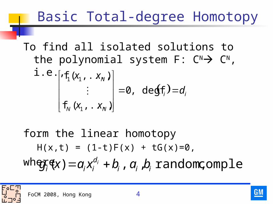
Basic Total-degree Homotopy

To find all isolated solutions to the polynomial system F: CN CN, i.e.,

form the linear homotopyH(x,t) = (1-t)F(x) + tG(x)=0,

where

ii

NN

N

d

xx

xx

fdeg ,0

),...,(f

),...,(f

1

11

complex random, , ,)( iiidiii babxaxg i


Polynomial Structures- The basis of “good homotopies”

(A) Start system solved with linear algebra

(B) Start system solved via convex hulls, polytope theory

(C) Start system solved via (A) or (B) initial run


Numerical Algebraic Geometry

Extension of polynomial continuation to include finding positive dimensional solution components and performing algebraic operations on them.

First conception Sommese & Wampler, FoCM 1995, Park City, UT

Numerical irreducible decomposition and related algorithms Sommese, Verschelde, & Wampler, 2000-2004

Monograph covering to year 2005 Sommese & Wampler, World Scientific, 2005


Slicing & Witness Sets Slicing theorem

An degree d reduced algebraic set hits a general linear space of complementary dimension in d isolated points

Witness generation Slice at every dimension Use continuation to get sets

that contain all isolated solutions at each dimension

“Witness supersets” Irreducible decomposition

Remove “junk” Monodromy on slices finds

irreducible components Linear traces verify

completeness


Membership Test


Linear Traces

Track witness paths as slice translates parallel to itself.

Centroid of witness points for an algebraic set must move on a line.


Real Points on a Complex Curve

Go to Griffis-Duffy movie…


Further Reading

World Scientific 2005


Regeneration

Building blocks Regeneration algorithm Comparison to pre-existing

numerical continuation alternatives


Building Block 1: Parameter Continuation

initial parameter space

target parameter space

Start system easy in initial parameter space Root count may be much lower in target

parameter space Initial run is 1-time investment for cheaper target

runs

Morgan & Sommese,

1989

To solve: F(x,p)=0


Kinematic Milestone

9-Point Path Generation for Four-bars Problem statement

Alt, 1923 Bootstrap partial solution

Roth, 1962 Complete solution

Wampler, Morgan & Sommese, 1992

m-homogeneous continuation

1442 Robert cognate triples


Nine-point Four-bar summary

Symbolic reduction Initial total degree ≈1010

Roth & Freudenstein, tot.deg.=5,764,801 Our reformulation, tot.deg.=1,048,576 Multihomogenization 286,720 2-way symmetry 143,360

Numerical reduction (Parameter continuation) Nondegenerate solutions 4326 Roberts cognate 3-way symmetry 1442

Synthesis program follows 1442 paths


Parameter Continuation: 9-point problem

2-homogeneous systems with symmetry:

143,360 solution pairs

9-point problems*:

1442 groups of 2x6

solutions

*Parameter space of 9-point problems is 18 dimensional (complex)


Building Block 2: Product Decomposition

To find: isolated roots of system F(x)=0 Suppose i-th equation, f(x), has the form:

Then, a generic g of the form

is a good start function for a linear homotopy.

Linear product decomposition = all pjk are linear.

s.polynomial all are where

,,,,)( 1111 1

(x)pp

ppppxf

jkjk

jkjk j

jjkjk ppppxg ,,,,)( 1111 1

Linear products: Verschelde & Cools 1994

Polynomial products: Morgan, Sommese & W. 1995


Product decomposition

For a product decomposition homotopy: Original articles assert:

Paths from all nonsingular start roots lead to all nonsingular roots of the target system.

New result extends this: Paths from all isolated start roots lead to

all isolated roots of the target system.


Building Block 3: Deflation Let X be an irreducible component of

V(F) with multiplicity > 1. Deflation produces an augmented

system G(x,y) such that there is a component Y in V(G) of multiplicity 1 that projects generically 1-to-1 onto X. Multiplicity=1 means Newton’s method can

be used to get quadratic convergence

Isolated points: Leykin, Verschelde & Zhao 2006, Lecerf 2002

Positive dimensional components: Sommese & Wampler 2005

Related work: Dayton & Zeng ’05; Bates, Sommese & Peterson ’06; LVZ, L preprints


Regeneration

Suppose we have the isolated roots of {F (x),g(x)}=0

where F(x) is a system and g(x)=L1(x)L2(x)…Ld(x)

is a linear product decomposition of f(x). Then, by product decomposition,

H(x,t)={F (x), γt g(x)+(1-t)f(x)}=0

is a good homotopy for solving {F (x),f(x)}=0

How can we get the roots of {F(x),g(x)}=0?


Regeneration

Suppose we have the isolated solutions of {F(x),L(x)}=0

where L(x) is a linear function. Then, by parameter continuation on the

coefficients of L(x) we can get the isolated solutions of

{F(x),L’(x)}=0.

for any other linear function L’(x). Homotopy is H(x,t)={F,γtL(x)+(1-t)L’(x)}=0.

Doing this d times, we find all isolated solutions of

{F(x), L1(x)L2(x)…Ld(x)} = {F(x),g(x)} = 0. We call this the “regeneration” of {F,g}.


Tracking multiplicity > 1 paths

For both regenerating {F,g} and tracking to {F,f}, we want to track all isolated solutions. Some of these may be multiplicity > 1.

In each case, there is a homotopy H(x,t)=0

The paths we want to track are curves in V(H) Each curve has a deflation. We track the deflated curves.


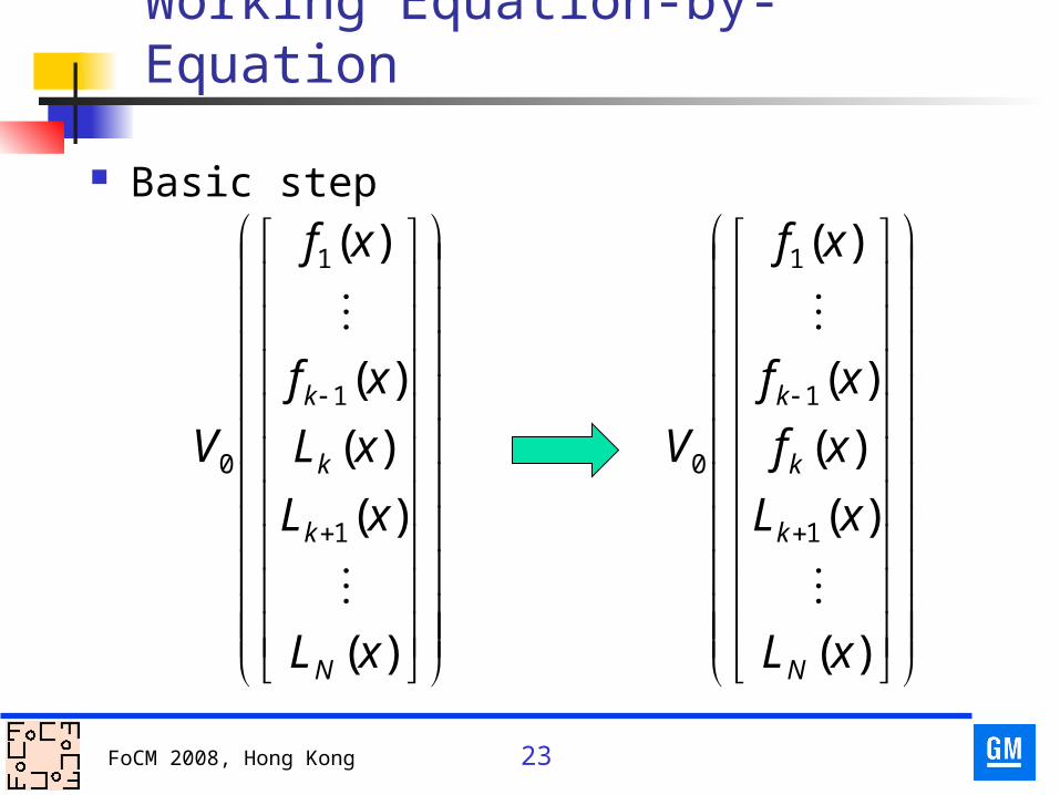
Working Equation-by-Equation

Basic step

)(

)(

)(

)(

)(

1

1

1

0

xL

xL

xL

xf

xf

V

N

k

k

k

)(

)(

)(

)(

)(

1

1

1

0

xL

xL

xf

xf

xf

V

N

k

k

k


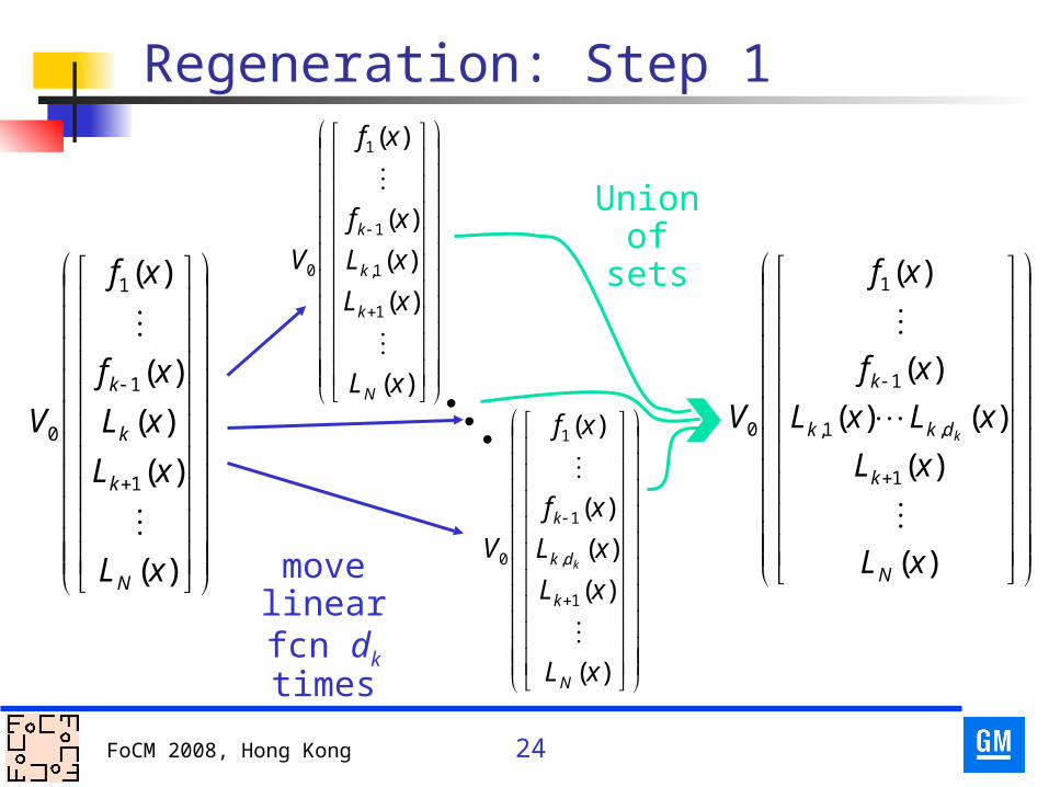
Regeneration: Step 1

)(

)(

)(

)(

)(

1

1

1

0

xL

xL

xL

xf

xf

V

N

k

k

k

)(

)(

)()(

)(

)(

1

,1,

1

1

0

xL

xL

xLxL

xf

xf

V

N

k

dkk

k

k

)(

)(

)(

)(

)(

1

1,

1

1

0

xL

xL

xL

xf

xf

V

N

k

k

k

)(

)(

)(

)(

)(

1

,

1

1

0

xL

xL

xL

xf

xf

V

N

k

dk

k

k

move linear fcn dk times

Union of sets


Regeneration: Step 2

)(

)(

)()(

)(

)(

1

,1,

1

1

0

xL

xL

xLxL

xf

xf

V

N

k

dkk

k

k

)(

)(

)(

)(

)(

1

1

1

0

xL

xL

xf

xf

xf

V

N

k

k

k

Linear

homotopy

Repeat for k+1,k+2,…,N


Equation-by-Equation Solving

f1(x)=0 Co-dim 1

f2(x)=0 Co-dim 1

f3(x)=0 Co-dim 1

Intersect

Co-dim 1,2

Co-dim 1,2,3

Co-dim 1,2,...,N-1

fN(x)=0 Co-dim 1Co-dim 1,2,...,min(n,N)

Final Result

Similar intersections

•Special case:•N=n•nonsingular solutions only•results are very promising

N equations, n variables

Intersect

Intersect

Theory is in place for μ>1 isolated and for full

witness set generation.


Alternatives 1

Polyhedral homotopies (a.k.a., BKK) Finds all isolated solutions Parameter space = coefficients of all monomials

Root count = mixed volume (Bernstein’s Theorem) Always ≤ root count for best linear product

Especially suited to sparse polynomials Homotopies

Verschelde, Verlinden & Cools, ’94; Huber & Sturmfels, ’95

T.Y. Li with various co-authors, 1997-present Advantage:

Reduction in # of paths Disadvantage:

Mixed volume calculation is combinatorial


Alternatives 2: Diagonal homotopy

Given: WX = Witness set for irreducible X in V(F) WY = Witness set for irreducible Y in V(G)

Find: Intersection of X and Y

Method: X × Y is an irreducible component of V(F(x),G(y)) WX × WY is its witness set Compute irreducible decomposition of the diagonal, x

– y = 0 restricted to X × Y Can be used to work equation-by-equation

Let F be the first k equations & G be the (k+1)st one Sommese, Verschelde, & Wampler 2004, 2008.


Other alternatives

Numerical Exclusion methods (e.g., interval

arithmetic) Symbolic

Grobner bases Border bases Resultants Geometric resolution

Here, we will compare only to the alternatives using numerical homotopy. A more complete comparison is a topic for future work.


Software for polynomial continuation

PHC (first release 1997) J. Verschelde First publicly available implementation of polyhedral method Used in SVW series of papers Isolated points

Multihomogeneous & polyhedral method Positive dimensional sets

Basics, diagonal homotopy Hom4PS-2.0 (released 2008)

T.Y. Li Isolated points:

Multihomogeneous & polyhedral method Fastest polyhedral code available

Bertini (ver1.0 released Apr.20, 2008) D. Bates, J. Hauenstein, A. Sommese, C. Wampler Isolated points

Multihomogeneous, regeneration Positive dimensional sets

Basics, diagonal homotopy Automatically adjusts precision: adaptive multiprecision


Test Run 1: 6R Robot Inverse Kinematics

Method* Work Time

Total-degree traditional

1024 paths

54 s

Diagonal eqn-by-eqn

649 paths 23 s

Regeneration eqn-by-eqn

628 paths 313 linear

moves

9 s

*All runs in Bertini


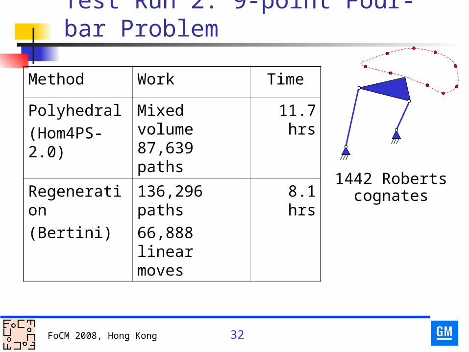
Test Run 2: 9-point Four-bar Problem

1442 Roberts cognates

Method Work Time

Polyhedral(Hom4PS-2.0)

Mixed volume 87,639 paths

11.7 hrs

Regeneration(Bertini)

136,296 paths66,888 linear moves

8.1 hrs


Test Run 3: Lotka-Volterra Systems

Discretized (finite differences) population model Order n system has 8n sparse bilinear equations Only 6 monomials in each equation

+ mixed volume

Work Summary

Total degree = 28n

Mixed volume = 24n is exact


Lotka-Volterra Systems (cont.)

Time Summary

xx = did not finish

All runs on a single processor


Summary

Continuation methods for isolated solutions Highly developed in 1980’s, 1990’s

Numerical algebraic geometry Builds on the methods for isolated roots Treats positive-dimensional sets Witness sets (slices) are the key construct

Regeneration: equation-by-equation approach Uses moves of linear fcns to regenerate each new

equation Based on

parameter continuation, product decomposition, & deflation Captures much of the same structure as polytope

methods, without a mixed volume computation Most efficient method yet for large, sparse systems

Bertini software provides regeneration Adaptive multiprecision is important

focm 2008, hong kong regeneration: a new algorithm in numerical algebraic geometry charles wampler...

Documents