fmri artifact correction in eeg and emg data titelderarbeit fmri artifact correction in eeg and emg...
TRANSCRIPT

Diplomarbeit
Titel der Arbeit
fMRI Artifact Correctionin EEG and EMG Data
Verfasser
Johann Glaser
Angestrebter akademischer Grad
Magister der Naturwissenschaften (Mag. rer. nat.)
Wien, 2012
Studienkennzahl: 298
Studienrichtung: Psychologie
Betreuer: Univ.-Prof. Dr. Claus Lamm und


Acknowledgment
I want to thank Prof. Claus Lamm and Florian Fischmeister, UniversityVienna, who supervised this diploma thesis. Florian advised me in the field ofEEG and fMRI data processing. He gave countless good hints and stimulatedcreative ideas.
I also want to thank my parents who enabled me to freely decide what tostudy and always supported me to reach my goals. The University Viennaprovided a good and fundamental education. The Institute of ComputerTechnology at the Vienna University of Technology was a very flexible em-ployer so I could schedule courses and pursue my study without an interrup-tion.
Special thanks go to the authors of EEGLAB with all its plugins, especiallythe FMRIB plugin. It provided the environment and the starting point formy work.
Kudos go to the worldwide open source community which develops numeroushighly professional tools. The tools I used most during my diploma thesisare: LATEX, BibTEX, TikZ, GNU Make, GVim, lots of other powerful GNUtools (sed, grep, ...), Linux, the GNOME desktop and many others. Thanksgo to their authors, maintainers, documenters, translators and all others whoare involved to provide these programs.
iii


Contents
1 Introduction 11.1 Multi-modal Imaging . . . . . . . . . . . . . . . . . . . . . . . . 2
1.1.1 Applications . . . . . . . . . . . . . . . . . . . . . . . . . 3
1.1.2 Electromyography . . . . . . . . . . . . . . . . . . . . . . 4
1.2 Challenges . . . . . . . . . . . . . . . . . . . . . . . . . . . . . 5
1.2.1 MR-Safety Aspects . . . . . . . . . . . . . . . . . . . . . 5
1.2.2 Interference . . . . . . . . . . . . . . . . . . . . . . . . . 6
1.3 Goal . . . . . . . . . . . . . . . . . . . . . . . . . . . . . . . . 6
2 Background 92.1 Methods . . . . . . . . . . . . . . . . . . . . . . . . . . . . . . 10
2.1.1 Magnetic Resonance Imaging (MRI) . . . . . . . . . . . . . 11
2.1.2 Functional MRI (fMRI) . . . . . . . . . . . . . . . . . . . 12
2.1.3 Electroencephalography (EEG) . . . . . . . . . . . . . . . 13
2.1.4 Electromyography (EMG) . . . . . . . . . . . . . . . . . . 14
2.1.5 Combined EEG/EMG with fMRI . . . . . . . . . . . . . . . 15
2.2 Artifacts . . . . . . . . . . . . . . . . . . . . . . . . . . . . . . 16
2.2.1 Electromagnetic Induction . . . . . . . . . . . . . . . . . . 17
2.2.2 Gradient Artifact Signal . . . . . . . . . . . . . . . . . . . 18
2.2.3 Ballisto-Cardiographic Artifacts (BCG) . . . . . . . . . . . 23
2.3 Artifact Correction Algorithms . . . . . . . . . . . . . . . . . . . . 24
2.3.1 Average Artifact Subtraction . . . . . . . . . . . . . . . . 25
2.3.2 FMRI Artifact Slice Template Removal (FASTR) . . . . . . 27
2.3.3 Realignment Parameter Informed Algorithm . . . . . . . . . 28
v

2.3.4 Retrospective Synchronization Algorithm (Resync) . . . . . . 29
2.3.5 fMRI Artifact Reduction for Motion (FARM) . . . . . . . . 30
2.3.6 Frequency Domain Template Removal . . . . . . . . . . . . 31
2.4 Performance Indicators . . . . . . . . . . . . . . . . . . . . . . . 33
2.4.1 Amplitude . . . . . . . . . . . . . . . . . . . . . . . . . . 33
2.4.2 RMS Ratios . . . . . . . . . . . . . . . . . . . . . . . . . 34
2.4.3 Signal to Noise Ratio . . . . . . . . . . . . . . . . . . . . 35
2.4.4 Analysis in Frequency Domain . . . . . . . . . . . . . . . . 37
2.4.5 Qualitative . . . . . . . . . . . . . . . . . . . . . . . . . 40
3 FACET — A New Correction Toolbox 433.1 Starting Point . . . . . . . . . . . . . . . . . . . . . . . . . . . . 44
3.1.1 EEGLAB, FMRIB Plugin . . . . . . . . . . . . . . . . . . 44
3.1.2 FARM Algorithm . . . . . . . . . . . . . . . . . . . . . . 44
3.2 Software Engineering . . . . . . . . . . . . . . . . . . . . . . . . 45
3.2.1 Reverse Engineering . . . . . . . . . . . . . . . . . . . . . 46
3.2.2 Software Re-Engineering . . . . . . . . . . . . . . . . . . . 47
3.2.3 Goals . . . . . . . . . . . . . . . . . . . . . . . . . . . . 47
3.2.4 Generalization . . . . . . . . . . . . . . . . . . . . . . . . 48
3.3 Object-Oriented Design . . . . . . . . . . . . . . . . . . . . . . . 49
3.3.1 Object-Oriented Design Paradigm . . . . . . . . . . . . . . 49
3.3.2 Software Design . . . . . . . . . . . . . . . . . . . . . . . 50
3.3.3 Algorithm Setup . . . . . . . . . . . . . . . . . . . . . . 52
3.3.4 Application Example . . . . . . . . . . . . . . . . . . . . 53
3.4 Data Analysis and Preparation . . . . . . . . . . . . . . . . . . . . 55
3.4.1 Analyze EEG Dataset and Setup . . . . . . . . . . . . . . 55
3.4.2 Get Trigger Latencies . . . . . . . . . . . . . . . . . . . . 57
3.4.3 Automatically Correct Missing Triggers . . . . . . . . . . . 57
3.4.4 Manually Correct Missing Triggers . . . . . . . . . . . . . . 57
3.4.5 Convert Volume to Slice Triggers . . . . . . . . . . . . . . 57
3.4.6 Test Data and Setup . . . . . . . . . . . . . . . . . . . . 58
3.5 Pre-Filter . . . . . . . . . . . . . . . . . . . . . . . . . . . . . . 58
3.5.1 Slow Fluctuations . . . . . . . . . . . . . . . . . . . . . . 59
3.5.2 High-Pass Filter Implementations . . . . . . . . . . . . . . 59
3.5.3 Low-Pass Pre-Filter . . . . . . . . . . . . . . . . . . . . . 60
3.6 Sub-Sample Alignment . . . . . . . . . . . . . . . . . . . . . . . 61
3.6.1 Problem . . . . . . . . . . . . . . . . . . . . . . . . . . 61
3.6.2 Time-Shift with Sub-Sample Resolution . . . . . . . . . . . 61
3.6.3 Interpolation Error . . . . . . . . . . . . . . . . . . . . . 62
3.7 Volume Artifact . . . . . . . . . . . . . . . . . . . . . . . . . . . 63
vi

3.7.1 Problem . . . . . . . . . . . . . . . . . . . . . . . . . . 63
3.7.2 Correction . . . . . . . . . . . . . . . . . . . . . . . . . . 64
3.8 Averaging Matrix . . . . . . . . . . . . . . . . . . . . . . . . . . 65
3.8.1 Generalization . . . . . . . . . . . . . . . . . . . . . . . . 65
3.8.2 Implementation . . . . . . . . . . . . . . . . . . . . . . . 67
3.9 Low-Pass Filter . . . . . . . . . . . . . . . . . . . . . . . . . . . 68
3.10 Algorithm Sequence . . . . . . . . . . . . . . . . . . . . . . . . . 69
3.10.1 Customization of Sequence . . . . . . . . . . . . . . . . . 69
3.10.2 Example . . . . . . . . . . . . . . . . . . . . . . . . . . 70
3.11 Evaluation Framework . . . . . . . . . . . . . . . . . . . . . . . . 72
3.11.1 Software Design . . . . . . . . . . . . . . . . . . . . . . . 72
3.11.2 Data Preparation . . . . . . . . . . . . . . . . . . . . . . 74
3.11.3 Performance Indicators . . . . . . . . . . . . . . . . . . . 74
3.11.4 Usage Examples . . . . . . . . . . . . . . . . . . . . . . . 76
4 Evaluation of EEGfMRI 79
4.1 Data . . . . . . . . . . . . . . . . . . . . . . . . . . . . . . . . 81
4.1.1 FMRIB Dataset . . . . . . . . . . . . . . . . . . . . . . . 81
4.1.2 Pilot Dataset . . . . . . . . . . . . . . . . . . . . . . . . 82
4.2 Comparison Without Post-Processing . . . . . . . . . . . . . . . . 83
4.3 Pre-Processing and Template Generation Improvements . . . . . . . 88
4.4 Incremental Activation of Post-Processing Steps . . . . . . . . . . . 95
4.5 Comparison with Post-Processing . . . . . . . . . . . . . . . . . . 100
4.6 Pilot Dataset . . . . . . . . . . . . . . . . . . . . . . . . . . . . 105
4.6.1 Comparison Without Post-Processing . . . . . . . . . . . . 105
4.6.2 Pre-Processing and Template Generation Improvements . . . 109
4.6.3 Incremental Activation of Post-Processing Steps . . . . . . . 115
4.6.4 Comparison with Post-Processing . . . . . . . . . . . . . . 119
4.7 Discussion . . . . . . . . . . . . . . . . . . . . . . . . . . . . . . 124
5 Summary 127
5.1 Artifact Correction and Evaluation Toolbox . . . . . . . . . . . . . 128
5.2 Future Work . . . . . . . . . . . . . . . . . . . . . . . . . . . . 129
References 131
Abstract 137
vii

Zusammenfassung 139
Curriculum Vitae 141
Lebenslauf 143
viii

1
Introduction
CONCURRENT acquisition of electroencephalogram (EEG) and func-tional magnetic resonance imaging (fMRI) is used since the late 1990ies.
This allows to combine the strengths of both methods and to complete thefragmentary information provided by either one of them.
These advantages also come with drawbacks like mutual artifacts. The gra-dient artifact due to rapidly changing magnetic fields induces voltage in theEEG signal which exceed the original signal by several orders of magnitude.Subtle movements of the subject also cause artifact voltages, which well ex-ceed the EEG signal. Although the drawbacks are tackled with broadlybased methods, the results are not perfect. Recently, not only EEG but alsoelectromyograph (EMG) signals are considered. While the acquisition equip-ment is similar, the signals are different and therefore pose new problems.Eventually, the remaining challenge is the motion of the subject.
This work compares existing methods to correct the EEG and EMG signalsand provides improvements to tackle these problems. The main outcome is auniversal toolbox, which provides methods for the removal of fMRI gradientartifacts from EEG and EMG signals.
1

2 Chapter 1. Introduction
1.1 Multi-modal Imaging
Both methods, EEG and fMRI, are used to investigate the working of thehuman brain. By the combination of these methods, the information on brainactivity is provided in two modalities. With the assumption that the signals“relate to the same event” and are “produced by the same neural generators”(Rosenkranz & Lemieux, 2010, p. 2), the methods provide complementaryinformation.
Originally, the combined acquisition of EEG and fMRI was used to localizethe sources of interictal epileptic neural activity by correlating the EEG signalwith the hemodynamic change observed by fMRI. From this initial clinicalexertion, the method has now gained numerous applications in neuroscience(Rosenkranz & Lemieux, 2010).
While fMRI is a non-invasive imaging technique covering the whole brainwith a high spatial resolution, it has a low temporal resolution. The relationbetween the vascular fMRI signal and the neural activity is expressed by theBOLD (blood oxygenation level dependent) response. This response functionis primarily unknown due to the influence of ongoing brain states and activity(Ritter & Villringer, 2006; Minati, 2006).
On the other hand, EEG monitors brain states and activities and additionallyhas a high temporal resolution. Its disadvantage is the low spatial resolutionand the fact, that the source can not be localized unambiguously (so calledinverse problem) (Ritter & Villringer, 2006; Minati, 2006).
Combining both methods allows to integrate the high temporal resolution ofEEG and the high spatial resolution of fMRI. By multi-modal data fusionthe inverse problem is solved (Rosenkranz & Lemieux, 2010).
According to Ritter and Villringer (2006), three combinations of EEG andfMRI are employed:
Conjoint acquisition records EEG and fMRI in separate sessions.
Interleaved acquisition is performed with the subject located inside ofthe fMRI scanner, but EEG and fMRI acquisition are performed atdifferent times.
Concurrent/continuous acquisition means, that fMRI and EEG are re-corded at the same time.
While conjoint acquisition does not pose any mutual influence of EEG andfMRI, it is not assured that the observed activities are related. The same

1.1 Multi-modal Imaging 3
disadvantage holds for interleaved acquisition, but due to the identical envi-ronment, the differences of cognitive processes are lower. However, the EEGand fMRI recording equipment might influence each other. For concurrentacquisition this problem is evidently given and is covered extensively in thiswork. Concurrent acquisition is the only variant which allows true multi-modal observation of brain processes (Ritter & Villringer, 2006; Menon &Crottaz-Herbette, 2005).
1.1.1 Applications of Multi-modal Imaging
For the investigation of spontaneous brain activity, the concurrent acquisi-tion of EEG and fMRI is mandatory. In cognitive and systems neurosciencethe coherence in this neural activity and the hemodynamic response is ob-served to study the idle state (also called the cognitive default mode) of thebrain (Rosenkranz & Lemieux, 2010; Ritter & Villringer, 2006). For examplethe driver and the spatial distribution of the classical human alpha-rhythmwere investigated. Studies reported by Ritter and Villringer (2006) showedreduced metabolism which is an indicator of inhibited cortical areas. Theorigin is highly likely the thalamus, but the results are still ambiguous dueto interfering rhythms from global state changes.
These global state changes, which even occur during rest, are reflected inBOLD signal fluctuations. To account for the additional variance in theBOLD signal, the state changes are observed with EEG and included asfactors in the statistical data analysis (Ritter & Villringer, 2006).
This approach is further extended to investigate evoked activity (Ritter &Villringer, 2006). The EEG signal recorded during repeated presentation ofstimuli is post-processed to acquire event related potentials (ERP). Featuresof the ERP are correlated to BOLD activity to “identify corresponding brainregions [...] at a timescale close to that of the EEG” (Rosenkranz & Lemieux,2010, p. 3)
Ritter and Villringer (2006) report works which correlate the time courseof EEG signal power in spectral bands electrode-wise with the BOLD sig-nal measured with fMRI voxel by voxel. Tightly synchronized inter-neuronsshowing gamma oscillations in the EEG signal are associated with an in-hibition as observed in the BOLD response, which at a macroscopic levelmeans that changes in spectral power are associated with BOLD changes(Rosenkranz & Lemieux, 2010).

4 Chapter 1. Introduction
Combined EEG and fMRI was also used to study the “relation between cog-nition/behavior and neuronal synchrony” (Ritter & Villringer, 2006, p. 833).Numerous studies found relations between EEG frequency contents and cog-nitive functions. The authors generally state, that “it would be of interestto create spatiotemporally resolved whole-brain maps of coherent neuronalnon-event-related activity for different behavior and cognitive states” (Ritter& Villringer, 2006, p. 834).
Besides the utilization of combined EEG and fMRI in research, the methodis also applied in clinical settings. For the treatment of epilepsy, the epilepticfoci are localized prior to the cortical resection (Ritter & Villringer, 2006;Rosenkranz & Lemieux, 2010). On the other hand, association of interictalepileptic electric activity with the hemodynamic response is not yet fully un-derstood (Ritter & Villringer, 2006) and intensively investigated (Rosenkranz& Lemieux, 2010). Electrical source imaging (ESI) is used to map the scalpEEG data to the three-dimensional locations in the brain to find the fo-cus of interictal epileptiform discharges and distinguish them from areas ofpropagation (Michel et al., 2004; Rosenkranz & Lemieux, 2010).
Ritter and Villringer (2006) summarize future utilization of the combinedacquisition of EEG and fMRI to better understand the high variability ofbrain responses and the dynamic coupling as well as to investigate the “age-related changes in brain physiology” (Ritter & Villringer, 2006, p.834).
1.1.2 Other Modalities: Electromyography (EMG)
In the previous sections possibilities for the combined acquisition of the twomodalities fMRI and EEG were outlined. Adding a third modality, namelyelectromyography (EMG), adds information on muscle activity like move-ments and strain (Fridlund & Cacioppo, 1986; Ritter & Villringer, 2006).
The recording equipment for EMG is very similar to that already in placefor EEG and can often be used for both purposes. The concurrent recordingof EEG and EMG during fMRI acquisition was shown in 1.5T and 3T MRscanners (Ritter & Villringer, 2006). Exemplary applications are the obser-vation of hand muscle activity (blocked hand) which showed no artifacts inthe MR image. Further more, maps of the sensorimotor system were assem-bled using concurrent fMRI, EEG and EMG (Ritter & Villringer, 2006). Forexample, van der Meer, Tijssen, Bour, van Rootselaar, and Nederveen (2010)observed the EMG activity on the neck, hand, and arm muscles during fMRIacquisition.

1.2 Challenges 5
1.2 Challenges
Although the combined acquisition of EEG and fMRI is in use for more thanten years, it still poses challenges. The main aspect is the safety of thesubject inside the MR scanner. The EEG leads act as antennas which pickup the RF excitation signal. This can lead to heating of the electrodes up tonearly 50C, although the mostly employed fMRI sequence EPI only leadsto an increase of less then 1C.
On the other hand, the mutual interference of both methods impair the ac-quired data. The influence of the EEG equipment to the MR image quality isnegligible when appropriate materials are chosen. However, the EEG signal isconsiderably deteriorated by electromagnetic induction due to minimal sub-ject movements and especially due to the rapidly changing gradient magneticfields.
1.2.1 MR-Safety Aspects
Besides the safety precautions for standalone-MR (Mühlenweg, Schaefers, &Trattnig, 2007) there are additional issues of the combination with EEG.The EEG electrode wires build resonant antennas which pick up the RFexcitation signal. This leads to heating and possibly burning of the subject’stissue (Meriläinen, 2002). Measurements of the temperature increase of EEGelectrodes in a 3T scanner performed on a phantom and a sheep head founda maximum temperature increase of 12.3C for the FSE sequence. This wasextrapolated to a steady state of 13.5C. For skin with a base temperature of36C this results in a temperature of 49.5C which causes burning and pain.
The temperature increase strongly depends on the specific absorption rate(SAR) of the MR sequence (FSE: 2.8W/kg, EPI: 0.077W/kg). The maxi-mum temperature increase measured with the EPI sequence, generally uti-lized for fMRI, was only 0.85C (Meriläinen, 2002). Unfortunately the studydid no systematic search for the spatial spot of the maximum temperatureincrease, so the measured value is a lower bound. Yet it suggests that at leastwith a 3T scanner no extreme temperature rise must be considered (Nöth,Laufs, Stoermer, & Deichmann, 2011).

6 Chapter 1. Introduction
1.2.2 Mutual Interference between EEG and fMRI
The combination of EEG and fMRI introduces mutual interference. Theseartifacts impair the acquired signal of both methods. The EEG equipmentattached to the subject affect the magnetic field due to its different magneticsusceptibility. This deteriorates the magnetic field homogeneity and thus theimage quality (Rosenkranz & Lemieux, 2010). Thus, appropriate selectionof materials to avoid ferromagnetic metals and to choose electrode gels andinsulators with low magnetic susceptibility is required. Furthermore, theEEG amplifier must withstand the high magnetic field and the fast gradientfields (Ritter & Villringer, 2006).
While the interference of EEG equipment to fMRI acquisition is negligible (atleast up to 3T), the artifacts introduced into the EEG signal are considerable.The underlying physical effect is electromagnetic induction; a change of themagnetic field induces voltages in the EEG leads (Ritter & Villringer, 2006).
Small movements of the subject change the position of the EEG leads andthus the portion of the static main B0 magnetic field they enclose. Due tothe high magnetic field, these artifacts are present as soon as the subjectis positioned inside the scanner bore, even without MR acquisition (Ritter& Villringer, 2006). These small movements caused e.g. by the pulsatingblood flow through the scalp cause the ballistocardiographic artifact (BCG)of more than 200µV (Allen, Polizzi, Krakow, Fish, & Lemieux, 1998).
The acquisition of MR images requires fast establishment of gradient mag-netic fields for spatial resolution. These changing magnetic fields cause muchhigher induction voltages in the EEG leads. Figure 1.1 shows a comparisonof a pure EEG signal with these gradient artifacts.
To reduce the induced voltages, the electrode wires need to be laid out witha minimum area of loops and special MR sequences with slowly changinggradient fields are applied (Ritter & Villringer, 2006).
1.3 Goal of this Work
Despite the effort to reduce the gradient artifacts induced in the electrodeleads, they still exceed the EEG signal by three to five orders of magnitude.These are corrected with mathematical algorithms which basically utilizetheir highly regular pattern. Multiple consecutive artifacts are averaged andsubtracted from the measured signal (Allen, Josephs, & Turner, 2000).

1.3 Goal 7
0 100 200 300 400 500 600 700 800−8
−6
−4
−2
0
2
4
6
8
t / ms
U/
mV
−10
0
10·10−3
Figure 1.1: Exemplary section of the FMRIB dataset (see Sec. 4.1.1) around theonset of fMRI acquisition. The amplitude of the pure EEG signal before the fMRIacquisition is below ±10µV (see inset). The acquisition starts at 338ms and causesgradient artifacts with an amplitude of ≈ ±8mV.
These algorithms work fine as long as the subject does not move. However,the acquisition of muscle activity with EMG is accompanied with (little)movements of the electrodes. These change the artifact signal pattern andthus pose problems to the existing algorithms.
The goal of this work is to evaluate existing correction algorithms and intro-duce improvements to cope with the challenges caused by subject movements.
The final outcome is to answer, whether it is possible to overcome current lim-itations of EEG/EMG measurements during fMRI acquisition. Additionallya proposal in the sense of “best practice” is given, which correction algorithmto select and how to adjust its parameters to obtain optimum results.


2
Background
THIS thesis is based on prior scientific work, as outlined in this chap-ter. Magnetic resonance imaging (MRI) is the underlying technique for
non-invasively acquiring structural information of the human brain. The socalled BOLD effect allows to exert this technique for functional inspection ofbrain activity (fMRI). Another functional method is electroencephalography(EEG), which measures electrical signals at the scalp surface and correlates itto stimuli and cognitive processes. EEG is often combined with electromyo-graphy (EMG) to measure muscle activity, e.g. of facial motion. Finally, thecombination of fMRI and EEG/EMG allows to complement the strengths ofboth methods and to cover the individual weaknesses.
However, mutual interferences of fMRI and EEG/EMG poses challenges tothe combined application. While the fMRI image quality is nearly unaffectedby the EEG recording, the EEG signals are severely impaired. Electromag-netic induction, caused by the rapidly changing MRI gradient fields, results ininterference several magnitudes larger than the EEG signal itself. The sameholds for artifacts caused by minor movements resulting from the cardiacpulse.
9

10 Chapter 2. Background
Multiple mathematical algorithms exist to remove the artifact. A very simpleimplementation zeroes the EEG signal during fMRI acquisition, but thisis only possible for MR sequences with short acquisition and long breaks.Most other algorithms utilize the high regularity of the gradient artifactand average multiple periods, which are then subtracted. The differencesbetween the algorithms are mainly in the pre-processing before and the post-processing after the average template subtraction. Another differentiationcan be found in the method of template generation. A few algorithms existwhich perform the correction in frequency domain.
All these correction algorithms obtain imperfect results. To assess the qualityof artifact removal, multiple performance indicators are employed. The sim-plest criteria is the signal amplitude, but also the root-mean-square (RMS)and the signal-to-noise ratio (SNR) are common. In frequency domain, theperiodic gradient artifact signal shows a fundamental and harmonics, whichare also used to assess the attenuation. Finally, qualitative measures are em-ployed, which on one hand are less reproducible, but are highly representativefor the further usage of the EEG signal.
2.1 Methods
Scientists and physicians were interested in the structures of the human brainfor a long time (Minati, 2006). Advances in technology allow to perform theseexaminations in-vivo with non-invasive methods. The most frequently uti-lized neuro-imaging techniques are computed tomography (CT) and magneticresonance imaging (MRI). Both methods reveal morphological informationof the brain (Minati, 2006).
Besides these morphological insight, techniques were developed which allowa functional analysis of the brain. MRI can easily be extended to functionalMRI (fMRI). A totally different physical approach is utilized by positronemission tomography (PET). While these methods are inherent imagingtechniques, the electrical brain activity is directly recorded only with elec-troencephalography (EEG). A related technology utilizes the magnetic fieldproduced by the electric activity, namely magnetoencephalography (MEG)(Minati, 2006).
EEG source localization techniques try to locate the generators of mea-sured features (Pascual-Marqui, Michel, & Lehmann, 1994; Pascual-Marqui,

2.1 Methods 11
1999; Baillet et al., 2001; Michel et al., 2004) which extend EEG to a (low-resolution) functional imaging technique.
The electrical activity of muscles is often recorded as an auxiliary measureto EEG (electromyograph, EMG). The recording of eye movement aids inEEG-post-processing to remove related artifacts (Fridlund & Cacioppo, 1986;Blumenthal et al., 2005). Besides this usage, EMG is also widely applied asstandalone method.
Although the mentioned functional imaging methods EEG and fMRI provideuseful information on their own, the combination allows deeper insights andprovides higher quality data. These multi-modal acquisition techniques com-plement each other to remedy each others shortcomings (Menon & Crottaz-Herbette, 2005; Ritter & Villringer, 2006; Rosenkranz & Lemieux, 2010).Alas, this comes at the price of mutual artifacts as will be discussed inSec. 2.2.
2.1.1 Magnetic Resonance Imaging (MRI)
Magnetic resonance imaging is a non-invasive imaging technique used in med-ical science to visualize tissue inside the body. It allows a comparable highspatial resolution (Minati, 2006).
The underlying physical principle utilizes the magnetic spin of the protons inatomic nuclei. These are aligned along a strong base magnetic field B0. AnRF field is used to deflect their rotation which leads to a precession aroundthe main axis. After this excitation, the relaxation occurs with a materialdependent time constant. This results in a contrast, i.e. the image intensity(Weishaupt, Köchli, & Marincek, 2003; Huettel, Song, & McCarthy, 2009).
The excitation has to be performed with a frequency which matches thenucleus resonance frequency (Larmor frequency). This linearly depends onthe magnetic flux density B. This fact is utilized for spatial coding to limitexcitation to certain regions of the body. During readout it is used to identifythe origin of the received signals by their frequency. The static base magneticfield B0 is homogeneous throughout the MR scanner. To setup a spatiallyvarying magnetic field, additional gradient fields are activated (Weishaupt etal., 2003; Huettel et al., 2009).
An MRI acquisition consists of of one or more RF excitations, gradient acti-vations and readouts. The precise temporal composition is called “sequence”.Many different variations are employed which allow to emphasize different

12 Chapter 2. Background
materials and physical effects. Since all sequences have their individualstrengths and weaknesses, the selection depends on the desired exploration.
With this methodology, the structures of the human body, especially of thebrain, can be visualized with high spatial resolution. Advanced methodsand according sequences exist to visualize the flow of blood (angiography),to visualize diffusion of liquid or to visualize the oxygenation level of blood(Minati, 2006). With the latter mechanism, a functional imaging approachis realized.
2.1.2 Functional MRI (fMRI)
With functional methods, the activity of the brain is studied. These areused to find the places of ongoing neural activity. Strictly speaking, there isno inactive state in brain, therefore an increase and decrease of activity isrecorded. Functional MRI (fMRI) is able to identify the regions with highspatial but low temporal resolution (Minati, 2006; Huettel et al., 2009).
The indicator of brain activity is the neural blood supply. Increased brainactivity results in raised metabolism and oxygen consumption which requireshigher blood supply. The regulation results in an excess supply which leadsto less desoxigenated venous blood, i.e., the blood after the consumers ismore oxygenated (Huettel et al., 2009; Ritter & Villringer, 2006).
The utilized physical effect is the dependence of the susceptibility of bloodon its oxygenation level. Oxygenated blood is diamagnetic while desoxy-genated is paramagnetic, which is a direct result of the molecular setup inthe hemoglobin. This varying susceptibility results in MR intensity con-trasts (blood oxygenation level dependence, BOLD effect, Ogawa, Lee, Kay,& Tank, 1990; Ogawa et al., 1993) which are used as an indicator of brainactivity (Ritter & Villringer, 2006).
The time course of the blood oxygenation in venous blood is delayed 3–8 seconds according to the hemodynamic response (Moser et al., 2010). Thisdepends on many factors (including the region of the brain) and can only beestimated mathematically (Huettel et al., 2009). An additional problem isthat no inference on neural activity is possible because the blood supply is“not regulated on the scale of individual neurons” (Ritter & Villringer, 2006,p. 825).
The fMRI analysis results in a sequence of voxel data of the whole brain. Anincrease (decrease) of the intensity value is interpreted as increase (decrease)in blood oxygenation and therefore as spots of neural activity (inhibition)

2.1 Methods 13
(Huettel et al., 2009). This shows low-frequency noise resulting from perma-nent and very slow large-scale fluctuations of blood supply, which origin ispoorly understood. On the other hand, event-related changes in blood sup-ply are investigated in more detail and build the basis for most fMRI studies(Menon & Crottaz-Herbette, 2005). Although the hemodynamic response isrelatively slow, the whole brain volume must be scanned with a period of afew seconds. This requires very fast MR sequences like echo planar imaging(EPI) (Huettel et al., 2009).
2.1.3 Electroencephalography (EEG)
With fMRI the brain activity is measured according to a secondary effect(blood oxygenation). Electroencephalography (EEG) directly measures theactivity as electrical signals at the scalp surface. This non-invasive tech-nique uses multiple electrodes placed at standard positions (10-20-system,see Bauer, 1984) connected to sensitive amplifiers. The amplitude is inthe range of only a few tens of micro-volts (µV) (Bear, Connors, & Par-adiso, 2007; Ritter & Villringer, 2006) with a maximum of 75µV (Menon &Crottaz-Herbette, 2005).
The “voltages [are] generated by the currents that flow during synaptic ex-citation of the dendrites of many pyramidal neurons in the cerebral cortex”(Bear et al., 2007, p. 587). “These currents induce voltage changes (in theuV range) that are smaller than action potentials but that last longer and ex-tend over a larger area of neural tissue.” (Menon & Crottaz-Herbette, 2005,p. 293). Only neural activity close to the scalp surface, i.e. the neo-cortex,can be recorded. The electrical activity of synchronized neurons sums up toa measurable signal (Bear et al., 2007; Ritter & Villringer, 2006; Menon &Crottaz-Herbette, 2005). This synchronization results in rhythmic activityeasily visible at EEG recordings. The frequency of these rhythms is dividedinto frequency bands (Bauer, 1984).
The electrical signal of the neurons has to pass the meninges and the skullwhich reduces its amplitude by a factor of 2 to more than 60 and “spatiallysmears the signals” (Ritter & Villringer, 2006, p. 824). Due to the low-pass property of cell membranes, only frequencies up to approximately 50Hzare conducted to the electrodes (Ritter & Villringer, 2006; Rosenkranz &Lemieux, 2010).
Due to the “spatial smearing” cited above, the EEG signal measured at theelectrodes is the sum of multiple sources, weighted by geometric and con-ductive properties of the head. This means that the sources are “projected”

14 Chapter 2. Background
to the scull surface. To identify the sources, the so called inverse problemhas to be solved, because for every actually measured signal pattern, “an infi-nite number of possible locations and magnitudes” (Ritter & Villringer, 2006,p. 825) of sources exist (Ritter & Villringer, 2006). Numerous algorithms andapproaches exist which try to identify the sources of the measured electricalactivity (see e.g. Pascual-Marqui et al., 1994; Pascual-Marqui, 1999; Bailletet al., 2001; Michel et al., 2004).
Besides recording the spontaneous EEG signal, many scientific experimentscorrelate the EEG signal as emerged after a stimulus. These recordingsare called event related potentials (ERP). The signal is immersed by therandom fluctuations of brain activity, so the signal-to-noise ratio (SNR) isbelow 1.0 (Menon & Crottaz-Herbette, 2005). To get a reasonable signal,many (hundred to thousand according to Bauer, 1984; 30–100 according toMenon & Crottaz-Herbette, 2005) recordings are averaged time locked to thestimulus onset. The “positive- [and] negative-going fluctuation[s] that can bevisually identified in the ERP waveform” (Menon & Crottaz-Herbette, 2005,p. 294) are given names depending on their ordinal position or latency afterstimulus onset (e.g., “P1”, “N400”). These components are used for furtherinvestigations.
A special class of ERPs are slow cortical potentials (SCP) which last up to10–20 s after the event. The frequencies are far below 1Hz and thus forbidthe usage of high-pass filters in EEG recording and processing (so calledDC-EEG) (Moser et al., 2010).
2.1.4 Electromyography (EMG)
Electromyography (EMG) is used to measure the strain and movement ofmuscles. “The EMG signal is a quasi-random train of motor unit actionpotentials discharged by the contraction of striate muscle tissue.” The signalranges “from fractions of a µV to several hundred µV” (Fridlund & Cacioppo,1986, p. 568) in a frequency range from several Hz to 2 kHz (ibd.).
The signal is picked up directly in the muscle with fine-wire or needle elec-trodes. It can also be measured non-invasively with surface electrodes at-tached to the skin above the muscles. A “paired electrode placement parallelto the course of the muscle fiber usually maximizes selectivity” (Fridlund &Cacioppo, 1986, p. 570).
EMG is often combined with EEG to monitor eye-blinks and eye movements(electrooculogram, EOG) (e.g. Iannetti et al., 2005). But it is also used

2.1 Methods 15
on it own, e.g., to study startle eye-blinks (Blumenthal et al., 2005) or armmovements (van der Meer et al., 2010).
2.1.5 Combined EEG/EMG with fMRI
The combined acquisition of EEG and fMRI allows to observe different indi-cators of the same activity at the same time. The “neural activity generat-ing EEG potentials or MEG fields increases glucose and oxygen demands”,that are the “basis for a spatial correspondence between fMRI responsesand HREEG/MEG source activity” (Babiloni et al., 2004, p. 1472). Withmulti-modal integration, “a more complete picture” and “deeper insights”(Rosenkranz & Lemieux, 2010, p. 2) to the activity of the brain are gained.Combined EEG and fMRI allow an “improved understanding of the spa-tiotemporal dynamics of brain activity” (Mulert et al., 2004, p. 1).
While EEG offers high temporal but low spatial resolution, fMRI offers highspatial resolution with low temporal resolution. The combination of bothmethods allows to compensate the individual drawbacks (Menon & Crottaz-Herbette, 2005; Ritter & Villringer, 2006; Rosenkranz & Lemieux, 2010;Babiloni et al., 2004).
It is important to note, that sources exist, which are only visible by onemodality. For example, there are many incoherently firing neurons of whichonly 1% are synchronous. This leads to a 30 times larger EEG signal butonly a small metabolic difference and therefore a small fMRI signal (Babiloniet al., 2004). Ritter and Villringer (2006) classifies this into three cases
• fMRI signal without EEG correlate (deep, tangential, self-canceling),• EEG signal without fMRI correlate (few synchronous neurons),• opposite EEG and fMRI signals (synchrony, spatial scales).
Despite these problems, experiments with voltage-sensitive dye and with in-vasive electrical recordings concurrently with fMRI show that a good relationbetween sources of EEG and fMRI exists (Babiloni et al., 2004). The “fMRIsignal is better correlated with the local field potential than with multiunitand single-neuron activity” (Menon & Crottaz-Herbette, 2005, p. 296), whichwas also shown in humans (Moser et al., 2010). Since the EEG reflects localfield potential it is save to assume that it has the same neural sources asfMRI (Menon & Crottaz-Herbette, 2005).
Several methods to combine the EEG and fMRI data (data fusion, multi-modal integration) are proposed. For single-trial EEG, the EEG signal isused as a covariate for the general linear model setup voxel by voxel of the

16 Chapter 2. Background
fMRI data. Averaged EEG (ERP) also allows to correlate the fMRI activationand the amplitude of ERP components. Additionally, the source localizationof ERP waveforms can be constrained by the spatial information of fMRIactivation (Menon & Crottaz-Herbette, 2005).
Inverse methods to locate the source of EEG activity show good precisionunder given conditions (Baillet et al., 2001; Michel et al., 2004). Mulert etal. (2004) performed source localization with the sole EEG data and founda mean Euclidean distance of the source of the P300-signal and the BOLDsignal of 16mm. Although this shows good concordance too, only minordisturbances in the EEG data can severely distort the source localizationand lead to uncertainty and ambiguity (Ritter & Villringer, 2006). ThereforeRitter and Villringer (2006) suggest to use “fMRI data as a partial constraint”(p. 830) for source localization. This requires a mathematical model (map-ping) of the cortex current dipole sources to the scalp potential distribution(modeling of forward problem) (Babiloni et al., 2004).
Although the concurrent data acquisition permits extended insights intobrain activity, the acquisition equipment causes mutual interference. Theartifacts in MRI images and fMRI data induced by the EEG recording areminimal or even don’t exist (Menon & Crottaz-Herbette, 2005). The influ-ence of the MRI scanner to the EEG data on the other hand can be quitelarge. These artifacts will be detailed in the following section.
Several studies corrected the artifacts or used a blocked design to avoid arti-facts for the significant sections of the EEG data. Only small differences toEEG recorded outside of the scanner were found (Menon & Crottaz-Herbette,2005). Mulert et al. (2004) found a slightly reduced amplitude of the N1 andP1 components, which also were observed a little earlier. The P300 compo-nent didn’t change in size. Bregadze and Lavric (2006) also compared theP3 component and didn’t find differences. According to Moser et al. (2010)the SCP amplitudes are slightly smaller and their locations are comparableto recordings outside the scanner. Therefore they conclude that it is feasibleto acquire DC-EEG in high magnetic fields (3T).
2.2 MR Artifacts in the EEG Data
The rapidly changing magnetic fields of the MRI acquisition (see Sec. 2.1.1)induce an electric voltage in the conductors of the EEG/EMG/ECG elec-trodes. These artifacts superimpose the biological signals. Their amplitude

2.2 Artifacts 17
is several orders of magnitude larger than EEG signals and thus completelyoverlay them. Before the artifact signal itself is analyzed, the physical prin-ciples of its origin are investigated.
2.2.1 Electromagnetic Induction
Given is a surface A as shown in Fig. 2.1 (Prechtl, 2006, p. 151, Fig. 9.1). Itsperimeter, denoted as ∂A, is the conductor of the electric circuit. A magneticflux Φ(A) is flowing through this surface. According to the law of induction,the voltage along the perimeter, i.e., in the electric circuit, U(∂A), equals thedecrease rate of the magnetic flux through the area (Prechtl, 2008, p. 109,eq. (20.1)).
U(∂A) = −Φ(A) (2.1)
A
∂A
Figure 2.1: Exemplary area A with perimeter ∂A.
To calculate the total magnetic flux Φ(A) through A, the surface is split intosmall pieces Ak. The total flux is the sum of the flux components throughthe small pieces. Each piece is assumed flat with the normal vector ~enk andlocal magnetic flux density ~Bk. The magnetic flux Φk through Ak is givenby the product the area Ak with the normal projection of the magnetic fluxdensity Bnk = ~Bk · ~enk: Φk = AkBnk. When further reducing the size of thepieces the sum converges to an integral and results in the compact formula(Prechtl, 2008, p. 16f, eq. (16.2))
Φ(A) =
∫ABn · dA. (2.2)
From eq. (2.2) two additive causes for a variation of the flux and thus of aninduced voltage according to eq. (2.1) are possible:
18 Chapter 2. Background
• The magnetic flux density ~B varies while the area A stays constant.This case applies to a changing magnetic field through a stationaryconductor.
• The area A changes its form or position within a constant magneticfield. This case is referred to as moving conductor.
Both effects apply in concurrent fMRI and EEG measurements: The gradientcoils constantly vary the magnetic flux density for spacial coding. Addition-ally small movements of the subject result in changes of the area spanned bythe EEG electrode cables.
2.2.2 Gradient Artifact Signal
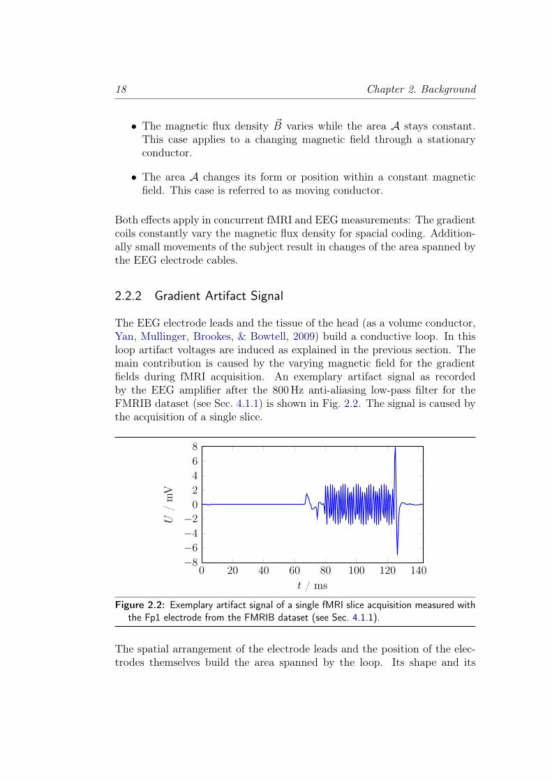
The EEG electrode leads and the tissue of the head (as a volume conductor,Yan, Mullinger, Brookes, & Bowtell, 2009) build a conductive loop. In thisloop artifact voltages are induced as explained in the previous section. Themain contribution is caused by the varying magnetic field for the gradientfields during fMRI acquisition. An exemplary artifact signal as recordedby the EEG amplifier after the 800Hz anti-aliasing low-pass filter for theFMRIB dataset (see Sec. 4.1.1) is shown in Fig. 2.2. The signal is caused bythe acquisition of a single slice.
0 20 40 60 80 100 120 140−8
−6
−4
−2
0
2
4
6
8
t / ms
U/
mV
Figure 2.2: Exemplary artifact signal of a single fMRI slice acquisition measured withthe Fp1 electrode from the FMRIB dataset (see Sec. 4.1.1).
The spatial arrangement of the electrode leads and the position of the elec-trodes themselves build the area spanned by the loop. Its shape and its

2.2 Artifacts 19
position relative to the magnetic field determine the amount and spatial dis-tribution of the “captured” magnetic flux. Together with its temporal varia-tion as defined by the MRI sequence, these factors define the exact artifactsignal. Therefore the artifact signal highly variates with the EEG electrodeposition (Yan et al., 2009). In Fig. 2.3 the artifact of all channels (i.e. EEG,EMG and ECG electrodes) of the FMRIB dataset (see Sec. 4.1.1) are shown.
This high spatial variability was investigated by Yan et al. (2009). Themaximum amplitude at any point of the scalp was determined in three ways.The voltage was calculated with analytical expressions assuming an idealpath of the electrode leads. Secondly, the digitized path of the electrodeleads was used for a numerical simulation of the voltages. Finally, the voltageswere measured during a combined EEG and fMRI acquisition with a speciallycrafted MR sequence.
With all three methods a high spatial variability was found. The valuesdetermined by both mathematical methods showed good correspondence tothe measurements. The analytical expressions were used to show that, dueto effects of the spherical wire paths, shifting and rotating the head resultsin a nonlinear increase or decrease of the artifact voltages. This informationwas used to minimize the artifact amplitude by optimizing the position insidethe bore.
The mathematical methods could be used to precisely model the artifactsignal and its variation due to the subject’s movement. Unfortunately thesignal strongly depends on the exact wire paths and the materials, especiallythe tissue of the subject’s head. Hence, it is far too complex to accuratelymodel it. However, these methods give a good opportunity to find generalrules how to reduce the artifact amplitude without sacrificing the qualityof the fMRI image and the EEG signal by the proper design of the wiringpatterns of EEG caps, placement of the subject in the bore, and so on.However, the measured artifact signal will not be modeled with an accuracyof µV.
Gradient Artifact Dimensions
The raw artifact amplitude strongly depends on the change rate of the mag-netic gradient field (which itself depends on the utilized fMRI sequence), theEEG electrode wire paths (loop area, orientation in the magnetic field), theEEG channel and the position of the head in the scanner (Yan et al., 2009).

20 Chapter 2. Background
−10
0
10
U/
mV Fp1 Fp2 F7 F3
−10
0
10
U/
mV Fz F4 F8 T3
−10
0
10
U/
mV C3 Cz C4 T4
−10
0
10
U/
mV T5 P3 Pz P4
−10
0
10
U/
mV T6 O1 O2 AF4
−10
0
10
U/
mV AF3 FC2 FC1 CP1
−10
0
10
U/
mV CP2 PO3 PO4 FC6
0 50 100−10
0
10
t / ms
U/
mV FC5
0 50 100
t / ms
CP5
0 50 100
t / ms
EMG
0 50 100
t / ms
ECG
Figure 2.3: Artifact signal shape of all 32 channels of the FMRIB dataset clearlyshowing the strong spatial variability.

2.2 Artifacts 21
The measured amplitude additionally depends on the analog input filter ofthe EEG amplifier1 and its input voltage range. Table 2.1 summarizes am-plitudes as reported by the given publications as well as of the data sets usedin this work.
Allen et al. (2000) assumed a gradient slew rate of 125 T/m·s (resulting in achange rate of 25 T/s at 0.2m distance from the isocenter) and a loop areaof 100 cm2 to calculate the raw artifact amplitude of 500mVpp. With a loopantenna they measured 25mVpp using a low-pass filter with a 3 dB cut-offfrequency of 70Hz (2nd order Bessel), which reduced the fast artifact com-ponents. Measurements of a human revealed EEG artifacts from 0.6mVpp
to 17.3mVpp and 16.3mVpp for the ECG channel. After digitally down-sampling and low-pass filtering with fc = 50 Hz, the artifacts were 114µVppto2980µVppwith a median of 571µVpp. Since these amplitudes are still muchlarger than biological signals, (Allen et al., 2000) conclude that a low-pass isnot enough to remove the artifacts.
For their simulation, Schlegelmilch, Schellhorn, and Markert (2004) used anartifact with an amplitude of 15mVpp as input for the presented correctionalgorithm. The measurements show an amplitude of 20mVpp.
Niazy, Beckmann, Iannetti, Brady, and Smith (2005) found a gradient artifactof 17mVpp using a 600 Hz, 1st order low-pass.
From the many calculated and measured amplitudes given by Yan et al.(2009), only those actually measured are shown here. The measurementswere performed with a well-defined gradient either in z or in x direction witha slew rate of 2 T/m·s. To reflect a more typical slew rate of 100 T/m·s, thevalues in Tab. 2.1 are scaled by a factor of 50.
A small artifact of 2.5mVpp is shown by Mandelkow, Brandeis, and Boesiger(2010) using a 250Hz low pass while van der Meer et al. (2010) show 22mVpp
with a similar filter.
From the FMRIB dataset as used in this work (see Sec. 4.1.1) the datashow amplitudes of 5.86mVpp to 25.6mVpp. The pilot dataset has muchlarger artifacts (117.1mVpp to 642.4mVpp) with only a slightly wider low-pass (800Hz instead of 600Hz).
1which is usually designed with a cut-off frequency below half of the sampling rate toavoid aliasing (Oppenheim, Willsky, & Nawab, 1997)

22 Chapter 2. Background
Table
2.1:Com
parisonof
artifactdim
ensions(o:1:1
storder,o:2:2
ndorder).
Referen
ceRan
geB
Low
-pass
min.
max.
median
Allen
etal.(2000)
calculated500.0
mV
pp
2T
measured
25.0m
Vpp
2T
70Hz
o:2largest
ECG
artifact16.3
mV
pp
2T
70Hz
o:2EEG
artifact0.6
mV
pp
17.3m
Vpp
4.0m
Vpp
2T
70Hz
o:2digitallow
-pass50
Hz
0.114m
Vpp
2.980m
Vpp
0.571m
Vpp
2T
70Hz
o:2Schlegelm
ilchet
al.(2004)sim
ulated15.0
mV
pp
1.5T
1200Hz
o:2measurem
ents20.0
mV
pp
1.5T
1200Hz
o:2Niazy
etal.(2005)
17.0m
Vpp
3T
600Hz
o:1Yan
etal.(2009)
phantom,z-gradient
5.0m
Vpp
3T
1000Hz
o:5phantom
,x-gradient
50.55m
Vpp
3T
1000Hz
o:5hum
anhead,
z-gradient24.8
mV
pp
3T
1000Hz
o:5hum
anhead,
x-gradient39.3
mV
pp
3T
1000Hz
o:5Mandelkow
etal.(2010)
2.5m
Vpp
3T
250Hz
vander
Meer
etal.(2010)
22.0m
Vpp
3T
250Hz
o:2FMRIB
dataset(Sec.4.1.1)
5.86m
Vpp
25.6m
Vpp
17.9m
Vpp
3T
600Hz
o:1Pilot
dataset(Sec.4.1.2)
117.1m
Vpp
642.4m
Vpp
408.8m
Vpp
3T
800Hz

2.2 Artifacts 23
2.2.3 Ballisto-Cardiographic Artifacts (BCG)
The source of the gradient artifacts is the variated magnetic flux during activefMRI acquisition generated by the gradient coils. The second source of aninduced voltage is the movement of the conductor in the static magnetic field(see Sec. 2.2.1). Even if the subject remains immobile, his pulsatile pulse flowinduces a pulse artifact (Allen et al., 1998).
Figure 2.4 shows an exemplary signal recorded inside of a 1.5T scanner beforethe fMRI acquisition. The pulse artifact has a “large amplitude peak followedby a complex waveform persisting throughout the interpulse period” (Allenet al., 1998, p. 230). It is recorded from almost all EEG electrodes andnormally has amplitudes from 10µV to 150µV with a large inter-individualvariability. Therefore it considerably perturbs the EEG acquisition.
0 2 4 6 8 10
−50
0
50
t / s
U/µV
Figure 2.4: Exemplary ballisto-cardiographic artifact measured with the F7 elec-trode after filtering with a bandpass from 2 to 10Hz from the FMRIB dataset(see Sec. 4.1.1) well before fMRI acquisition onset.
Two sources are responsible for the pulse artifact. First, the small pulse-related body movements of the head and the expansion and contraction ofscalp arteries lead to variation of the EEG electrode wire positions and there-fore to an induced voltage in these conductors (Allen et al., 1998) propor-tional to B0 (Debener, Mullinger, Niazy, & Bowtell, 2008). Secondly, as theblood itself is a conductive fluid, its flow generates the blood flow effect.When blood in a vessel flows perpendicular to the B0 field, a voltage perpen-dicular to the flow and B0 is induced. Its amplitude is proportional to B0,its velocity v and the orientation of the vessel relative to B0 and reverselyproportional to the distance to the EEG electrode (Kolin, 1952).

24 Chapter 2. Background
Debener et al. (2008) found large spatial variation of the BCG and suggeststhe removal channel by channel, e.g. utilizing the ICA. Niazy et al. (2005)calculated a PCA for the BCG artifact occurrences and used the first 3 PCsas template to be subtracted.
The methods to reduce pulse artifacts from EEG data are widely spread,therefore the BCG artifact is not further considered in this work.
2.3 Artifact Correction Algorithms
As summarized in Tab. 2.1, the amplitude of the gradient artifact exceeds theamplitude of EEG and EMG signals by several orders of magnitudes. Theremoval is therefore a non-trivial task. Filtering with low pass is not enough,because frequency components of the artifact overlap with the frequencies ofinterest for EEG and EMG signals (Allen et al., 2000).
Several algorithms to remove the artifacts were proposed. Goldman, Stern,Engel, and Cohen (2000) used an fMRI sequence with a slice acquisitionduration of 90ms followed by 580ms without gradient activity. In the EEGdata post-processing the periods of slice acquisition were zeroed, leaving ausable portion of the signal of 87%. This high fraction was usable for theirstudy, but a zeroed signal is not acceptable for other studies.
Within every channel, the artifact signal shape is a periodic function for theacquisition of every fMRI slice and/or volume (see Fig. 2.5). Many algorithmsutilize this fact to calculate an artifact template (e.g. by averaging all sliceartifacts) and subtract (Allen et al., 2000).
0 50 100 150 200 250 300 350 400 450 500 550−8−6−4−202468
t / ms
U/
mV
Figure 2.5: Exemplary section of the FMRIB dataset (see Sec. 4.1.1) with four con-secutive fMRI slice acquisition periods measured with the Fp1 electrode. It is clearlyvisible that the shape of the slices are very similar.

2.3 Artifact Correction Algorithms 25
This template subtraction paradigm still leaves residual artifact signals whichare larger than the biological signals (Allen et al., 2000). Therefore thecalculation of the template is optimized and several pre-processing and post-processing steps are added by many authors. Figure 2.6 shows a generalizedscheme for this group of algorithms (see also Sec. 3.2.4).
Pre-Processing
Template Subtraction TemplateGeneration
Post-Processing
Figure 2.6: General approach of the artifact correction algorithms.
Within the next sections the following algorithms will be described in detailincluding their advantages and disadvantages:
• Sub-sample grouping (Bénar et al., 2003)• Interpolation–template–alignment–subtraction (ITAS) (Ritter, Becker,
Graefe, & Villringer, 2007)• Image artifact reduction (Allen et al., 2000)• fMRI artifact slice template removal (FASTR) (Niazy et al., 2005)• Realignment parameter informed algorithm (Moosmann et al., 2009)• Retrospective synchronization algorithm (Mandelkow et al., 2010)• fMRI artifact reduction for motion (FARM) (van der Meer et al., 2010)
The processing of these algorithms is performed in time domain. Addition-ally the following algorithms will be outlined, which perform correction infrequency domain:
• Median power spectrum subtraction (Sijbers et al., 1999)• Comb filter (Hoffmann et al., 2000)• Frequency-domain filters (Hoffmann et al., 2000)
2.3.1 Average Artifact Subtraction
A simple implementation of the template subtraction paradigm calculates asingle template by averaging all epochs. Several factors diminish the success

26 Chapter 2. Background
of this approach. The following sections present these factors as well asproposed solutions by published algorithms.
Sub-Sample Grouping
The begin of an fMRI volume and/or slice acquisition is not synchronizedwith the EEG sampling. For example, at a sampling rate of 1 kSps, i.e. asampling period of 1ms, the start of one slice can be 0.1ms before an EEGsampling, the next slice could start at 0.3ms after the EEG sampling.
Bénar et al. (2003) divided the EEG sampling interval into ten partitions.Every epoch (EPI volume) was assigned to one of these ten bins, depend-ing on the exact start of the MR acquisition relative to the EEG sampling.Finally, individual templates for every bin were calculated and subtracted.
This approach reduces the problem arising from unsynchronized fMRI andEEG acquisition. The problem is not corrected perfectly, because only tenbins were used, which still left remaining uncertainties. Since the templatewas built from epochs all over the long exploration, the authors reportedproblems with movements of the subject.
Interpolation-Template-Alignment-Subtraction (ITAS)
The problem of a missing synchronization between the fMRI acquisition andthe EEG sampling was also considered by Ritter et al. (2007). Contrary tocalculating separate templates for every individual sub-sample offset, theyaligned every epoch to maximize its cross-correlation with a reference epoch.This alignment was performed with an up-sampled data and then down-sampled again.
The template was calculated by averaging all epochs, but using a weightedsum which attenuated epochs with higher distance. This reduces the impactof changes of the artifact waveform. Similar to Bénar et al. (2003), theinterpolation was performed in discrete steps which leaves uncertainties.
Block-wise processing
If the data shows a small drift or if the subject has moved during the acqui-sition, the calculated template will not fit well for any epoch. This results ina high residual artifact.

2.3 Artifact Correction Algorithms 27
To avoid this problem, the template generation and subtraction is performedblock-wise by Allen et al. (2000). The template was calculated by averagingn consecutive epochs and then subtracted from them. This was repeatedwith every next n epochs.
To further reduce the impact of atypical epoch signals, the averaging didn’tnecessarily include all n epochs. After the first five epochs were averaged, theremaining epochs were added iteratively, but only if their cross-correlationto the current average exceeded 0.975.
For an fMRI EPI sequence which had short gaps between the acquisitionof every volume, the whole volume was used as an epoch, of which n = 25were averaged per block. Additionally, for two subjects a continuous fMRIsequence without gaps between volumes was acquired. This allowed to choosethe slices as epoch and a block length of n = 100.
The resulting signal was filtered with a high order low-pass with fc = 80Hzand down-sampled to 200 Sps. The EEG signal still contained residual ar-tifacts with approximately 30–50µV. Therefore a post-processing step withadaptive noise cancellation (Widrow et al., 1975) was applied to the data.To generate the reference signal, pulses at the epoch timing instances werefiltered with the same low-pass as the EEG signal (Allen et al., 2000).
The use of short periods (blocks) for the template generation as well as theexclusion of atypical epochs greatly reduces the impact of subject movement.The problem of missing synchronization was tackled by recording the slicetime with a higher resolution of 10µs than the EEG sampling period of 200µs(5 kSps). The EEG was up-sampled using a sinc-interpolation (Oppenheim etal., 1997, p. 523) before template calculation, similar to Ritter et al. (2007).This reduced the sampling problem but the block-wise processing still doesnot provide a satisfying solution for movement artifacts. The first five epochsin each block have an outstanding impact on the template, because all furtherepochs are excluded if not similar enough.
2.3.2 FMRI Artifact Slice Template Removal (FASTR)
The FMRI artifact slice template removal (FASTR) algorithm was intro-duced by Niazy et al. (2005) and Iannetti et al. (2005). Similar to Allenet al. (2000), it uses triggers from the MR scanner which indicate the slicetiming. The difference is that here the triggers have the same temporalresolution as the EEG sampling.

28 Chapter 2. Background
As the title indicates, the algorithm calculates templates for every slice ofthe EPI sequence. To tackle the problem of unsynchronized acquisition,the EEG data is up-sampled by a factor of 10. While Ritter et al. (2007)performs a time-shift of the data and then down-sample it again, here thetrigger indices are adjusted within the refined time resolution and furtherprocessing is performed before down-sampling.
After applying a 1Hz high-pass filter to reduce baseline effects of slow drifts,the artifact template is calculated as a local moving average of a configurablenumber of slice segments before and after the current one. Only every secondslice is used so that the EEG signal is uncorrelated between slices. Thistemplate is multiplied by a factor to minimize its squares to the segment.
The next stage is the first post-processing step (compare Fig. 2.6). The prin-cipal component analysis (PCA) is used to calculate a set of basis functionsfor the residuals. Those components describing the most variance (calledoptimal basis set (OBS) by Niazy et al., 2005), are again scaled to minimizethe squared error and added to the artifact template signal from the previousstage which is then subtracted from the EEG signal.
In the next step, this estimated error signal and the EEG signal with theartifact templates subtracted are down-sampled and filtered by a 70Hz low-pass. Similar to Allen et al. (2000), as a second post-processing step, adaptivenoise cancelling (ANC) is used with the reference being the estimated errorsignal.
The algorithm tackles the problem of unsynchronized sampling and fMRIclocks, but only with a limited quantization equal to the up-sampling fac-tor. This still leaves considerable residual artifacts. Calculating the slicetemplates using a moving average (instead of block-wise, like Allen et al.,2000) assigns identical influence to every epoch and adopts to slow changesof the artifact signal. However, sudden movements of the subject poison thetemplate of all surrounding epochs. The new post-processing step using aprincipal component analysis greatly removes residual artifacts.
2.3.3 Realignment Parameter Informed Algorithm
The previous algorithm uses a moving average to calculate the artifact tem-plate. This solves the problem of slow drifts of the artifact shape (Moosmannet al., 2009). Still problematic is the case, when an abrupt change of the ar-tifact signal occurs. While a movement of the subject of 1.5mm is reported

2.3 Artifact Correction Algorithms 29
for 30% of all recordings, a displacement of 1mm already impairs the resultof Allen et al. (2000) (Moosmann et al., 2009).
The calculated artifact template is an average of the shape before and of theshape after the abrupt change. The two regions “pollute” the template andlead to suboptimal results. Therefore, the data before and after the abruptchange “should not be used together to form one template” (Moosmann etal., 2009, p. 1146).
Moosmann et al. (2009) use the fMRI realignment parameters calculatedfrom the image data, which specifies the head displacement and rotationfrom one volume acquisition to the next. If the movement exceeds a certainthreshold, the EEG data during this interval is not used for the calculationof the artifact template. Furthermore, these points define barriers for thesliding average algorithm.
The algorithm reduces the impact of subject movements to the EEG signal,but requires data from the fMRI pre-processing.
2.3.4 Retrospective Synchronization Algorithm (Resync)
The problem of unsynchronized clocks of the EEG recording system andthe MR scanner was tackled by several procedures already covered above.Mandelkow et al. (2010) introduce the retrospective synchronization of theEEG data to the MR scanner clock. The de-synchronization factor D
D =round(TR · FS)
TR · FS
(TR: MR repetition time, FS: EEG sampling rate) expresses the factor bywhich the EEG sampling frequency is off an integer multiple of the MRrepetition time and is near one D ≈ 1.
Instead of calculating the value from the (unknown) TR and FS, it is esti-mated from the EEG data by maximizing the cross correlation of a time-shifted version of the artifact. The resynchronized signal is calculated withan inverse Fourier transform with the interpolation factor D. Contrary to thepreviously mentioned algorithms, all calculations are performed in frequencydomain and thus avoid up-sampling of the data.
This algorithms introduces new methods to tackle unsynchronized EEG andfMRI acquisition. On the other hand, no special measures are taken to avoidproblems with subject movement.

30 Chapter 2. Background
2.3.5 fMRI Artifact Reduction for Motion (FARM)
All algorithms presented so far work well with EEG but experience difficultieswith motion. The inherent motion involved with measuring EMG leads toinduced voltage during the movement as well as an altered shape of theartifact signal due to the different layout of the conductive loop (compareSec. 2.2.1).
A correction algorithm specifically for EMG data was presented by van derMeer et al. (2010). It is largely based on the algorithm by Niazy et al.(2005) (see Sec. 2.3.2) and adds several improvements and adoptions to beapplicable for EMG data. In the pre-processing step (compare Fig. 2.6) a30Hz high-pass is added, since the frequency range of EMG data is from30Hz to 250Hz.
One major improvement is to consider fMRI sequences which include a shortgap between every volume acquisition. At this points, the volume artifact ispresent, which also extends into the slice artifacts before and after the gap. Itis replaced by synthesized data which is calculated from slice artifacts morethan one slice away. Additionally, the slice timing as well as the durationfor the gap are estimated. Contrary to Niazy et al. (2005), the slice markersare not quantized with the (up-sampled) sampling frequency but calculatedwith a sub-sample resolution, similar to Ritter et al. (2007).
The template generation is improved by using a larger sliding window of 50slices, but choosing a set of 12 artifacts with the highest correlation to thecurrent artifact. In the post processing step, the data is filtered with a 250Hzlow-pass to conserve the frequencies of interest for EMG (Niazy et al. (2005)uses a 70Hz low-pass). The final ANC applied by Niazy et al. (2005) is notused by van der Meer et al. (2010).
By choosing the epochs with the best fit to the current epoch, a well suitedtemplate is generated. It most probably does not contain epochs with subjectmovement or with an altered shape of the artifact due to changed positionof the electrode leads. The synchronization problem is solved by shiftingthe epoch temporally with a sub-sample resolution. However, the algorithmis strongly tailored to EMG data and removes frequency components below30Hz. In this range important EEG information is present.

2.3 Artifact Correction Algorithms 31
2.3.6 Frequency Domain Template Removal
While the algorithms outlined up to this point perform the signal processingin time domain, the following approaches work in frequency domain. Therepetitive application of the gradient fields leads to a periodic artifact sig-nal. In frequency domain this corresponds to a discrete frequency and itsharmonics (Oppenheim et al., 1997). Hoffmann et al. (2000) systematicallyinvestigated the sources of multiple frequency components originating fromby fMRI acquisition. These come from the periods of the volume, the slice,and the readout gradient fields.
Median Power Spectrum Subtraction. Sijbers et al. (1999) divided theEEG data into sections with a length of TR (for slow imaging sequences) anda length of multiple TRs for fast imaging sequences (resulting in a length of150 to 300ms). The latter was necessary because the artifacts lasted longer,i.e. decayed slower, than TR and therefore superimposed with the followingartifacts.
For each section the power spectrum was calculated and averaged using asliding window median filter of 15 sections for slow and 31 sections for fastimaging sequences. This template was scaled to minimize the mean squarederror to the current interval and subtracted. Finally an inverse Fourier trans-form was performed to calculate the cleaned EEG signal.
This algorithm was evaluated for the standard imaging MR sequences SpinEcho (SE), Gradient Echo (GE) and Diffusion Weighted (DW) but not forEPI. The subject was an anesthetized rat, so no movement related problemsare expected. The experiment was performed with a 7T scanner with a80mm bore.
The acquisition of the EEG and the artifact was performed in two separatesessions. The EEG was recorded with the anesthetized rat but without MRacquisition, while the artifacts were recorded using a dead rat. The input forthe artifact reduction algorithm was the sum of the EEG and the artifact sig-nal. This allowed to compare the corrected signal with the true uncorruptedsignal.
As performance indicator the authors introduced the signal-to-artifact ratiowhich is defined as the standard deviation of the pure EEG signal divided bythe standard deviation of the residual or full artifact. Note that although thedefinition resembles the SNR (see Sec. 2.4.3), it relates signal RMS valuesinstead of the signal power values.

32 Chapter 2. Background
The recorded artifact was very small with an RMS of only 29% to 71% ofthe EEG signal RMS. After the application of the correction algorithm, theresidual artifact was 7% to 18%, respectively (Sijbers et al., 1999).
As the authors report, the correction algorithm is based on the power spec-trum. This removes the phase information in frequency domain and thusleads to signal distortion in time domain. Due to the small dimensions of arat’s head, only small wire loops and therefore small gradient artifact voltageswere observed. The authors did not show the performance of the algorithmfor larger artifact voltages.
Comb Filter. The algorithm of Sijbers et al. (1999) does not depend on thepreviously mentioned periodicity of the MR artifacts, because it calculates afrequency domain template for the whole spectrum. Contrastingly, Hoffmannet al. (2000) used a comb filter with narrow notches at the slice frequencyand its harmonics as well as one volume frequency above and below them.This was implemented in time domain with FIR filters (Oppenheim et al.,1997). Although no quantitative evaluation, the corrected signal allowed theidentification of epileptic spike waves. The applied comb filters have a finitestop band attenuation. Due to the high amplitude of the gradient artifactsignal, considerable residual artifacts are expected.
Frequency Domain Filter. For a greater reduction of the artifact am-plitude, the filtering can be performed in frequency domain by setting theamplitude to 0.0 at the according frequency bins (Hoffmann et al., 2000).
The implementation was split into two parts. Firstly, an averaged andsmoothed spectrum of an unaffected EEG was calculated. Secondly, ev-ery amplitude of the corrupted EEG signal, which exceeded the value of theunaffected EEG by more than 50%, was set to zero. This approach againdoes not rely on the knowledge of the MR sequence repetition times.
Bénar et al. (2003), who also used this approach, reported severe ringing atblock boundaries, due to the ideal filter characteristic (Oppenheim et al.,1997).

2.4 Performance Indicators 33
2.4 Performance Indicators
To assess the quality of results after the application of a correction algorithm,multiple criteria were employed. In this section, these are summarized andgrouped by their underlying physical or numerical property.
The following performance indicators are investigated:
• Amplitude– Median Imaging Artifact
• RMS– RMS Corrected to Unimpaired– RMS Uncorrected to Corrected
• SNR– Pseudo-SNR– Exact SNR from Correlation
• Frequency Domain– Median Residual Activity.– Power Density at Slice Frequency– Spectrograms– Residual Normalized Error Power– Average Spectrum– Surrogate Biosignal Preservation
• Qualitative– Epileptiform Spike-waves– α-Rhythm– BCG Artifact– ECG Quality– Principal Component Analysis
2.4.1 Amplitude
The simplest physical property is the sole signal amplitude, summarized withthe median.
Median Imaging Artifact. Allen et al. (2000) calculate the median imag-ing artifact for the raw EEG data, two intermediate steps, and the final cor-

34 Chapter 2. Background
rected data. Therefore “[...] the mean of 10 measurements, made at equallyspaced intervals [...], was calculated for each channel.” This mean value wascalculated for every channel, subject and recording, from which finally themedian value was taken. Although the publication does not specify what ismeant by “measurement”, it is assumed that it specifies the range (i.e. peakto peak value) of the EEG data within an interval of a length slightly overthe fMRI slice time.
The final comparison showed a “500-fold reduction” of the signal amplitudefrom 4.0mVpp with the artifacts to 8.0µVpp with the artifacts removed.Although the reduction shows the efficacy of the correction algorithm, itdoes not show whether the resulting signal amplitude is comparable to anon-corrupted EEG signal.
2.4.2 RMS Ratios
The Root-Mean-Square value (RMS) is the quadratic mean of a signal andis defined for a continues time signal x(t) and discrete time signal xi by
xRMS =
√1
T
∫ T
0
x2(t)dt =
√√√√ 1
n
n∑i=1
x2i , (2.3)
respectively. It is the square-root of the signal power because the signalvalues are squared. Apart from the signal mean (i.e, the DC value) it isidentical to the (biased) standard deviation of the signal (Glover & Grant,2004).
RMS Corrected to Unimpaired. One “evaluation metric” of Moosmannet al. (2009) is the standard deviation of the corrected signal, compared tothe standard deviation of the physiological EEG signal during artifact freeperiods. This performance indicator represents the fraction of the correctedto the pure signal. If the ratio is greater than 1, residual artifacts are stillpresent while values below 1 show that the correction algorithm removedparts of the wanted signal.
RMS Uncorrected to Corrected. van der Meer et al. (2010) comparetheir algorithm with the algorithm of Niazy et al. (2005) by calculating theratio between the RMS of uncorrected EMG periods and artifact-correctedEMG periods. The bigger this ratio the better, i.e., the more artifact was

2.4 Performance Indicators 35
removed, but the same problem as noted in Sec. 2.4.1 applies here too: Thisvalue doesn’t show whether the algorithm has removed too much of the signal.In this case van der Meer et al. (2010) use the ratio to show that theiralgorithm removes more of the artifacts than Niazy et al. (2005) do.
2.4.3 Signal to Noise Ratio
The Signal to Noise Ratio (SNR) relates the power of a wanted signal tothe power of a superimposed noise signal. The SNR of a distorted signalx(t) = xS(t) + xN(t) or xi = xS,i + xN,i is defined as the power S of theundistorted signal xS(t) or xS,i divided by the power N of the noise xN(t) orxN,i (Lee & Messerschmitt, 2000)
SNR =S
N=
∫ T
0
x2S(t)dt∫ T
0
x2N(t)dt
=
n∑i=1
x2S,i
n∑i=1
x2N,i
, (2.4)
for continues time and discrete time signals, respectively. It is usually con-verted to decibel (dB) due to the large dynamic range of the value
SNRdB = 10 log10
(S
N
). (2.5)
Note, that the definition relates the signal power values, which are the squareof the signal RMS values (compare eqn. 2.3).
Pseudo-SNR. Moosmann et al. (2009) added a surrogate single trial ERP(Quiroga & Garcia, 2003) to the raw EEG data and compared it to the ERPafter artifact correction. A 5Hz 7µV sine with random time jitter was used.The authors define the SNR as
SNR =
[cov (ERPoriginal,ERPcorrected)
σERPoriginal· σERPcorrected
]2(2.6)
= corr (ERPoriginal,ERPcorrected)2
(see eq. (9) on p. 1147), i.e. by squaring the correlation coefficient of theoriginal and the corrected signal.

36 Chapter 2. Background
Exact SNR from Correlation. The calculation of the SNR from thecorrelation coefficient with equation (2.6) (Moosmann et al., 2009) is only anapproximation for low values of the correlation coefficient. This can easilybe validated since the range of that value would be 0–1 which does not coverthe range of a real SNR.
For an exact derivation let the original signal x(t) be modeled as a wide-sensestationary random process X(t) (Weinrichter & Hlawatsch, 1991). Its signalpower is given by S = EX(t)2 where E· is the expected value (Lee &Messerschmitt, 2000, p. 50).
The cross-correlation of two real, zero-mean and jointly wide-sense stationaryrandom processes X(t) and Y (t) is given by RXY (t, τ) = EX(t)Y (t − τ).The Pearson correlation coefficient ρXY (t) is derived from RXY (t, τ) by set-ting τ = 0 and dividing by the standard deviations σX =
√EX(t)2 and
σY =√EY (t)2 (Lee & Messerschmitt, 2000, p. 55ff). Substitution finally
gives the expression for the correlation coefficient
ρXY (t) =EX(t)Y (t)√EX(t)2EY (t)2
. (2.7)
Two new signals X1(t) = X(t) + η1(t) and X2(t) = X(t) + η2(t) result fromX(t) by the addition of two different zero-mean noise signals η1(t) and η2(t)(again wide-sense stationary random processes). Their power is given byNi = Eηi(t)2. X(t), η1(t) and η2(t) are mutually uncorrelated.
The correlation coefficient (Borga, 2001)2 of the two signals X1(t) and X2(t)with arbitrary amplification by the factors a and b, respectively, is given by(the time parameter (t) is omitted for better readability)
ρ =Ea(X + η1) · b(X + η2)√
E a2(X + η1)2 · E b2(X + η2)2
=EX2√
(EX2+ Eη21) · (EX2+ Eη22)
=S√
(S +N1)(S +N2). (2.8)
For the special case3 that the first signal equals the original signal (i.e. η1 = 0,N1 = 0) and the second signal is the corrupted signal (the “noise” corresponds
2http://www.imt.liu.se/~magnus/cca/tutorial/node10.html [2012-01-05]3http://www.imt.liu.se/~magnus/cca/tutorial/node12.html [2012-01-05]

2.4 Performance Indicators 37
to the error (signal) introduced by the correction algorithm), the correlationcoefficient simplifies to
ρ =S√
S(S +N). (2.9)
From this equation, the signal-to-noise ratio SNR can be derived as
SNR =S
N=
ρ2
1− ρ2 . (2.10)
For low values of ρ the denominator approaches one
limρ→0
(1− ρ2
)= 1
and thus (2.10) simplifies to SNR ' ρ2, which is identical to (2.6).
As assumed by Moosmann et al. (2009), the SNR of the ERP signal afterthe application of their artifact correction algorithm can be calculated fromnumeric data. However, while in their case high values for the correlationcoefficient ρ with the original surrogate ERP signal are desired, the utilizedformula (2.6) is only an approximation for low values of the correlation co-efficient ρ. Therefore the exact formula (2.10) should be used.
2.4.4 Analysis in Frequency Domain
Various evaluation criteria were used by different authors which partly inves-tigate EEG signal frequency bands and others investigate fMRI acquisitionfundamental and harmonic frequencies.
Median Residual Activity. The mean activity in four representativeEEG frequency bands (0.8–4Hz (Delta waves), 4–8Hz (Theta waves), 8–12Hz (Alpha waves) and 12–24Hz (part of the Beta wave spectrum)) wascalculated by Allen et al. (2000). Therefore the average spectrum from ten5.12 s periods (i.e., 1024 samples at 200 Sps) was determined for every chan-nel and subject. Then the mean activity in every frequency band of thecorrected signal (AIAR) was compared to the mean activity during no fMRIacquisition (ANI) by calculating the absolute value of the relative differencein percent
Percentage Difference = 100 %×∣∣∣∣AIAR − ANI
ANI
∣∣∣∣ .

38 Chapter 2. Background
To summarize the percentage difference values, the median (due to non-normality) for all channels and subjects was determined. This performanceindicator is a measure for the deviance of the corrected signal in EEG fre-quency bands.
Power Density at Slice Frequency. For the evaluation of their algo-rithm, Niazy et al. (2005) calculated the spectral power density at the slicefrequency fundamental and harmonics. They compared the values for thedata before, for some intermediate steps of the algorithm and for the finaloutput. These indicate the attenuation of the fMRI noise base frequency andits harmonics achieved by the artifact correction algorithm.
For the practical calculation of the power spectral density the data is trans-formed from time domain to frequency domain with a discrete Fourier trans-form (DFT).4
Only periodic signals which exactly fit into the total DFT length, i.e. whichhave an integer number of periods, result in a single frequency bin. Sig-nals with a non-integer number of periods also contribute to neighboringfrequency bins. This so called “Leakage effect” (Doblinger, 2001; Glover &Grant, 2004) also was reported by Niazy et al. (2005). However, they didn’tfurther consider the considerable amount of signal power outside of the mainbins of the slice frequency and its harmonics.
The disregarded leaked signal power can lead to a substantial error in thecalculation of the slice frequency power density. This problem is reducedby the fact, that the comparison was performed between the values of theoriginal signal and the corrected signal, which both had the same leakageconditions.
A second problem arises from the width of the frequency bins, which is in-versely proportional to the total length of the signal. Therefore the evaluationof the correction result of an acquisition with a short fMRI activity has widerfrequency bins and therefore higher spectral power values than a dataset witha long fMRI session. Again, since the comparison is performed between twoequal length datasets, the problem equally applies to both and is cancelled.
Spectrograms. The visual representation of the time course of power spec-tral density of a signal is called spectrogram (see Fig. 2.7 for an example).
4For the calculation of a DFT usually the FFT (fast Fourier transform) is used, whichis a very efficient implementation of the algorithm (Oppenheim et al., 1997; Doblinger,2004).

2.4 Performance Indicators 39
This is used by van der Meer et al. (2010) to visualize the decreased powerat slice harmonics achieved by their correction algorithm, compared to thealgorithm of Niazy et al. (2005). Although the underlying data enables aquantitative analysis, the authors only suggest visual inspection.
0 20 40 60 80 100 120 140 1600
50
100
150
200
250
300
Time / s
Freq
uenc
y/
Hz
Figure 2.7: Exemplary spectrogram with a frequency resolution of 1Hz and temporalresolution of 0.5 s. It shows the spectral contents of the FMRIB dataset aftercorrection with the algorithm presented by Niazy et al. (2005) (the hotter the colorthe more activity).
Residual Normalized Error Power. Mandelkow et al. (2010) calculatethe power spectral density of the corrected signal Scorrected(f) and of thebaseline signal without fMRI acquisition Swithout(f). The normalized powerspectral density is then calculated by Scorrected(f)/Swithout(f). The residual erroris given by subtracting the expected value 1. The power C|f2f1 is calculatedby summing up along the frequency from f1 to f2.
C|f2f1 =
f2∑f=f1
∣∣∣∣Scorrected(f)
Swithout(f)− 1
∣∣∣∣The residual normalized error power is calculated for six frequency bands(< 20Hz, < 40Hz, < 90Hz, < 190Hz, < 690Hz, < 990Hz) and visualizedas stacked bar graphs. This performance indicator is very similar to themedian residual activity (Allen et al., 2000) above. Instead of 5.12 s periods

40 Chapter 2. Background
it uses the whole signal, and calculates the signal power in different frequencybands.
Average Spectrum. For every subject, the EEG acquisition data withoutacquisition, with acquisition, and after correction was split into 120 epochsof 8000 samples (1.6 s) (Ritter et al., 2007). For every epoch the FFT wascalculated and averaged for each of the three cases separately. One numberfor each of six frequency bands corresponding to EEG bands was calculated(presumably by summing the frequency domain values). These numbers werecompared in three ways: a) corrected without fMRI acquisition vs. correctedwith fMRI acquisition, b) corrected with fMRI acquisition vs. uncorrectedwithout fMRI acquisition and c) corrected without fMRI acquisition vs. un-corrected without fMRI acquisition.
Surrogate Biosignal Preservation. Ritter et al. (2007) added six con-tinuous sine waves with certain frequencies from 3Hz to 120Hz and an am-plitude of 100µV to the EEG data set. After performing the investigatedartifact correction algorithms, the resulting data was visualized with spec-trograms. The evaluation of the preservation of the surrogate signals wasdone by visual inspection.
2.4.5 Qualitative Performance Indicators
Besides the mathematical evaluation, there are also methods which require ahuman reviewer to rate the data. Although these methods cannot be used asreproducible and reliable performance indicators (Mandelkow et al., 2010),they often represent the practical usage of the corrected data (e.g. Allen etal., 2000).
Epileptiform Spike-waves. Spike-waves, recorded from a subject withepilepsy, were added to the raw EEG data of the healthy subjects at randomtimes (Allen et al., 2000). This data was then corrected with their algorithmand reviewers had to identify these spike-waves. The proportion of correctlyidentified was used as an indicator of the quality of the corrected data.
α-Rhythm. Allen et al. (2000) and Niazy et al. (2005) identified α-rhythmin the corrected data and compared the channel and frequency to recordingsof the same subject outside the scanner.

2.4 Performance Indicators 41
BCG Artifact. The presence of BCG artifacts, which show a distinctshape, equal with and without an active fMRI acquisition, were requiredto be present after the artifact removal by Niazy et al. (2005).
ECG Quality. The ECG signal has a unique shape. Niazy et al. (2005)asked reviewers to classify the quality of the features in the ECG signal afterthe artifact removal.
Principal Component Analysis. Mandelkow et al. (2010) used a prin-cipal component analysis (PCA) and visually inspected the leading principalcomponents whether they are similar to the residual gradient artifact as wellas “their contribution to the overall variance” (p. 2294).


3FACET — A New
Correction Toolbox
BASED on the algorithms summarized in Sec. 2.3 a new universal andflexible toolbox with improved artifact correction results is developed.
This toolbox is called “FACET – A Flexible Artifact Correction and Eval-uation Toolbox”. The algorithm by Niazy et al. (2005) is used as startingpoint. With the process of software re-engineering the Matlab code is reim-plemented with the object-oriented design paradigm. This enables flexibility,maintainability and extensibility.
Dedicated tools for the analysis of the EEG input data as well as methodsto correct faulty trigger recordings are implemented. Multiple algorithmicimprovements are introduced which lead to an extended correction of theartifacts. To allow the flexible configuration of the algorithm and to ensurereproducible results, the setup and execution is guided by a configuration fileinstead of a graphical dialog. The toolbox is complemented by a dedicatedframework for the evaluation of artifact correction algorithms using selectedperformance indicators as summarized in Sec. 3.11.3.
The goal is to provide a flexible toolkit which allows to combine algorithmcomponents as required to acquire the best artifact correction results. Theseshould surpass the quality of existing algorithms.
43

44 Chapter 3. FACET — A New Correction Toolbox
3.1 Starting Point
This work is mainly based on the correction algorithms by Niazy et al. (2005)and van der Meer et al. (2010).
3.1.1 EEGLAB, FMRIB Plugin
The FASTR algorithm published by Niazy et al. (2005) (see also Sec. 2.3.2) isavailable as a plugin1 for the widely used EEG processing tool kit EEGLAB2
(Delorme & Makeig, 2004). EEGLAB is a program for Matlab3 and is freesoftware (open-source) under the terms of the GNU General Public License(GPL)4. This permits the free distribution of the software as well as allmodifications thereof, given its source code is included.
To execute the FMRIB plugin, the user is offered a dialog window withseveral parameters (see Fig. 3.1). Although the labels are descriptive, it istedious and error prone when performing the algorithm multiple times. Theactual algorithm is a Matlab function with up to 13 parameters to configureits behavior (see Lst. 3.1).
This Matlab function is written in one long piece (1106 lines)5. Only five ex-ternal functions (apart from standard Matlab functions) are used. The mainpart is a loop over the EEG channels with a body of 470 lines performing theactual template generation and subtraction, PCA and ANC. Most variablenames are shortened and used without a description. Of the total 1106 lines,only 169 use a comment of which only 60 are related to code documentation.
3.1.2 FARM Algorithm
For the FARM algorithm (van der Meer et al., 2010) no code is available.Although several EMails were sent to the corresponding author, he didn’tsend an answer. Therefore only the descriptions as available in the articlewere used for the implementation of the algorithm.
1http://www.fmrib.ox.ac.uk/eeglab/fmribplugin/2http://sccn.ucsd.edu/eeglab/3http://www.mathworks.com/4http://www.gnu.org/licenses/old-licenses/gpl-2.0.html5sometimes pejoratively denoted as “spaghetti code”, http://en.wikipedia.org/wiki/
Spaghetti_code

3.2 Software Engineering 45
Figure 3.1: Screenshot of the FMRIB Plugin setup dialog.
3.2 Software Engineering
Software development is ideally performed in three steps: At the beginningthe requirements are summarized as a specification. This is the startingpoint for the program implementation, which mainly involves programming.Finally, the implemented program needs to be validated to ensure meetingthe specification and to sort out errors (Sommerville, 2004).
The final program is then deployed and set to operation. However, this isnot the end of development: To remain useful, maintenance of the programhas to be performed. This includes fault repair, adaption, and the additionor modification of functionality (Sommerville, 2004).
The task of this thesis includes such a software evolution process: The algo-rithm as provided by the FMRIB plugin has to be adapted and functionalityhas to be added. To start with, “[...] the process of system evolution involvesunderstanding the program that has to be changed [...]” (Sommerville, 2004,p. 501). Ideally this should be supported by a full specification and fore-sighted planning with extensibility and maintainability in mind.

46 Chapter 3. FACET — A New Correction Toolbox
Listing 3.1: Section of the FMRIB plugin implementing the FASTR algorithm (Niazyet al., 2005) from fmrib_fastr.m.
function EEG=fmrib_fastr(EEG,lpf,L,window,Trigs,strig,anc_chk,...
tc_chk,Volumes,Slices,varargin)
% ...
% EEG: EEGLAB data structure
% lpf: low-pass filter cutoff
% L: Interpolation folds
% window: length of averaging window in number of artifacts
% Trigs: An array of slice triggers locations.
% strig: 1 for slice triggers, 0 for volume / section triggers.
% anc_chk: 1 to do Adaptive noise cancellation
% 0 to not.
% tc_chk: 1 to correct for missing triggers, 0 for not
% Volumes: FMRI volumes for use in trigger correction
% Slices: FMRI Slices / Volume for use in trigger correction
% varargin1: relative position of slice trigger from beginning of
% slice acquisition: 0 for exact start -> 1 for exact end
% default=0.03;
% varargin2: Channels not to perform OBS on.
% varargin3: Numer of PCs to use in OBS. use 0 to skip this step.
% ’auto’ or empty for auto order selection.
% ...
“However, many systems, especially older legacy systems [...], aredifficult to understand and change. The programs may have beenoriginally optimised for performance or space utilisation at theexpense of understandability, [...]” (Sommerville, 2004, p. 501)
3.2.1 Reverse Engineering
As stated above, this also applies to the implementation of the FASTR cor-rection algorithm (Niazy et al., 2005). Although their article is a well writtenspecification of the algorithm, the actual implementation diverges at severalpoints. Additionally, the source code itself is poorly documented, optimizedfor memory usage, and was not planned with maintainability in mind (com-pare Sec. 3.1.1).
Therefore, a prerequisite and first step was reverse-engineering the program(Sommerville, 2004). Its source code was analyzed to understand the func-

3.2 Software Engineering 47
Check input and initialize parametersExtract triggers and correctPrepare internal variables and filtersAlign slice triggers according to first channelFor every channel: Construct artifact and subtract
Up-sample dataCalculate average artifact and subtractCalculate PCA of residuals and subtractDown-sample dataFilter with low-passAdaptive noise cancellation
Print duration of execution
Figure 3.2: Structogram of the implementation of the FASTR algorithm (Niazy et al.,2005) in the EEGLAB FMRIB plugin.
tionality, the data (i.e., variables), and its organization. Figure 3.2 showsa structogram of the implementation of the FMRIB algorithm. In parallel,documentation was added to the code.
3.2.2 Software Re-Engineering
As a second step, the process of software re-engineering was utilized to in-crease the maintainability (Sommerville, 2004). This included the renamingof variables to more understandable names and improvements of the struc-ture. Additionally, several simplification were performed, although at theexpense of higher memory demand. In each of these cycles, special care wastaken to keep the functionality and architecture unchanged by permanentvalidation and verification of the results.
3.2.3 Goals
In the course of software reverse-engineering and re-engineering, the algo-rithm of Niazy et al. (2005) and its implementation were understood. Thisestablished a basis to define the goals of the improved artifact correctionalgorithm.

48 Chapter 3. FACET — A New Correction Toolbox
The first goal is to build a universal and powerful toolbox, yet easy touse, with algorithms for the correction of gradient artifacts from EEG datarecorded during fMRI acquisition.
As a second goal, this toolbox should be implemented using modern softwaredesign paradigms with understandability, maintainability and extensibilityin mind.
Thirdly, the toolbox should provide an extensive set of utilities for data anal-ysis, preparation, filtering and correction. These should include functionalityas already published (Niazy et al., 2005, van der Meer et al., 2010, Allen etal., 2000, Moosmann et al., 2009 and others).
The fourth goal is to provide a mechanism to use a flexible combination ofthese utilities. This should still be executed in an automated process tominimize user interaction and to maximize reproducibility of the results.
Fifth, and most important, the toolbox should be demonstrated by imple-menting an improved algorithm which gives better results than establishedalgorithms like Niazy et al. (2005).
Therefore, as a sixth goal, the toolbox should include an evaluation frame-work which allows to analyze the results of the correction algorithm usingmultiple performance indicators (see Sec. 2.4).
Finally, the toolbox should be released as free software under the terms ofthe GNU General Public License6 for public download.
3.2.4 Generalization
The generalized scheme for artifact reduction algorithms proposed in Sec. 2.3and Fig. 2.6 is repeated here for reference (see Fig. 3.3). Reverse-engineeringthe source code of the FMRIB plugin revealed a structure very similar tothe generalized scheme (see Fig. 3.2). The algorithm by van der Meer et al.(2010) also fits in this scheme, although no source code was available.
While Niazy et al. (2005) interpolates the EEG data by a default factor of10 and corrects the slice trigger markers to the finer temporal resolution,van der Meer et al. (2010) use a temporal shift of every slice period with asub-sample resolution. These pre-processing steps are introduced to avoidinaccuracies and thus residual artifacts in the following template subtractionstep.
6http://www.gnu.org/licenses/old-licenses/gpl-2.0.html

3.3 Object-Oriented Design 49
Pre-Processing
Template Subtraction TemplateGeneration
Post-Processing
Figure 3.3: General approach of the artifact correction algorithms.
The template generation step of Niazy et al. (2005) implements nested loopsto average n epochs before and after the current epoch, with only everysecond epoch included (i.e. sliding window). On the other hand, van derMeer et al. (2010) use a subset of n epochs of a larger number surroundingthe current epoch which have the highest similarity to the current epoch (i.e.best candidates).
Niazy et al. (2005) and van der Meer et al. (2010) use a very similar post-processing with PCA and ANC. Additionally, van der Meer et al. (2010) fillthe volume gaps with synthesized data.
3.3 Object-Oriented Design
The process of software re-engineering includes source code translation. Thisinvolves the conversion to a more modern version and design paradigm of theprogramming language (Sommerville, 2004).
The implementation of the FMRIB plugin utilizes a procedural design para-digm, where all functionality is divided into self-contained sub-routines. Theprocessed data is supplied as input parameters and returned as output pa-rameters. This architecture was re-engineered to the object-oriented designparadigm (Sommerville, 2004). This paradigm was selected to utilize itsspecific advantages of data encapsulation, maintainability and extensibility.
3.3.1 Object-Oriented Design Paradigm
“An object is an entity that has a state and a defined set of operations thatoperate on that state.” (Sommerville, 2004, p. 316). In other words, an

50 Chapter 3. FACET — A New Correction Toolbox
object is a container, which stores all parameters and data (“state”). Addi-tionally it has associated methods, which perform operations on that object,i.e. on its parameters and data. While the word “object” denotes an actualinstance, the definition of its data (also called “fields”) and its methods isspecified by the so called “class”.
During design specification the classes and their relationships are visualizedusing the Unified Modeling Language (UML) class diagrams (Sommerville,2004, p. 316). Every class is drawn as a rectangle with the class name inthe top portion. This is followed by the fields and the methods, which areannotated to express their visibility (i.e. the access permissions like private,public, ...). Inheritance, instantiation and all other relationships are denotedby arrows with defined tips and labels.
Although Matlab itself is a procedural language, the support for object ori-ented programming was introduced with version 7.6 (R2008a). Differingnames are used for fields, which are termed “properties”.
3.3.2 Software Design
For the artifact correction toolbox, no advantageous points were identifiedto split the data and/or functionality into multiple classes. Therefore a sin-gle class “FACET” was created to hold all parameters and data. Its methodsoperate on this data to perform the artifact correction. Besides the dataencapsulation, no other object oriented concepts like inheritance and poly-morphism are used. Figure 3.4 shows the UML class diagram.
Public member fields for parameters and the EEG data are placed in theclass. These have to be set by the user after instantiation of the class. Forsome of these fields, setter methods are used to extract derived values fromthe assigned parameters. These are stored to member fields with publicread-only accessibility.
Keeping the EEG data (which by far requires the largest amount of memory)inside the object as a member variable also improves memory management.In contrast, Niazy et al. (2005) used functions and handed over the EEGdata as function parameter and return value. In this case, Matlab creates acopy of the data every time. In the object-oriented approach, all methodswork on the object member variables, therefore no copy is performed. Thisleads to reduced memory requirements and faster execution.
Several public methods are provided to analyze the data and remove theartifact. First of all, the constructor FACET() creates a new instance of the

3.3 Object-Oriented Design 51
FACET
EEGExcludeChannelsSliceTriggerRelTrigPosAutoPreTrigVolumeGapsInterpolateVolumeGapsAlignSlicesReferencePreFilterLPFrequencyPreFilterHPFrequencyPreFilterHFrequenciesPreFilterHAmplitudesPreFilterGaussHPFrequencyRASequenceUpsampleUpsampleCutoffSSAHPFrequencyAvgWindowAvgMatrixAvgMatrixUpdaterDataOBSNumPCsOBSExcludeChannelsOBSHPFrequencyFinalLPFrequencyDoANCDontTouchNonArtifactProfiling
FACET()FindTriggers()AnalyzeData()FindMissingTriggers()AddTriggers()GenerateSliceTriggers()CheckData()Prepare()PreFilter()RemoveArtifacts()Finish()
Figure 3.4: Class diagram of the FACET base class of the artifact correction toolbox.Only the public fields and methods are shown and the method parameters and returnvalues are omitted.

52 Chapter 3. FACET — A New Correction Toolbox
class. Other methods are used to identify (and optionally correct) triggerevents and to print an analysis of the EEG data. Finally, the core algorithmis performed by executing its associated methods.
The internal working is split into multiple private and protected methods.Additionally, events are issued at important points of execution to notifyany interested programs. This allows, e.g., to modify the data or to printprogress reports during the algorithm execution.
Visual output. The central class FACET silently performs the algorithmand does not print anything to the screen. The above mentioned eventsare used by the derived class FACET_Text, which inherits from FACET (seeFig. 3.5). It registers listeners to every event and prints a short message forevery notification.
FACET
...
FACET()...
FACET_Text
FACET_Text()...
Figure 3.5: Class diagram of the FACET_Text class, which prints a textual progressreport of the artifact correction algorithm.
Package. All classes (including the evaluation framework, see Sec. 3.11)are put together in the Matlab package FACET (note: it has the same name asthe class of the correction toolbox).
3.3.3 Algorithm Setup
The original FASTR algorithm was configured with a graphical dialog (seeFig. 3.1). As stated above, for multiple invocations of the algorithm, thisis tedious and error prone. The dialog is a front-end for the Matlab func-tion fmrib_fastr(), which is called with up to 13 input parameters (seeLst. 3.1). This can be directly called by the user and therefore guarantee

3.3 Object-Oriented Design 53
identical settings for multiple invocations. On the other hand, there is nodirect possibility to document and to justify the chosen values.
A configuration file is an alternative to the dialog and to the direct commandentry. The user sets options and parameters for the algorithm before it isexecuted. It should allow user comments, so that he can put notes on theentered information like description of the configuration values and rationalefor decisions. Therefore, a configuration file guarantees reproducible anddocumented results.
Using the object-oriented paradigm and employing Matlab itself as a scriptinglanguage enables the setup of the algorithm in exactly this way. Instead ofa pure configuration file, a Matlab script or function is used. It can bedocumented with comments to the users desire. The configuration valuesare assigned to public properties of the FACET object. Here the full powerof Matlab is available to determine the value, either as a direct value, orcalculated with user-defined formulas and even functions.
3.3.4 Application Example
The algorithm setup and execution should be demonstrated by an example.The toolbox provides several examples in the files CleanEx1.m to CleanEx6.m
(short for “cleaning example number 1–6”) which will be used in excerptsthroughout this work to demonstrate the features of the toolbox. The ex-ample CleanEx1.m uses the FMRIB dataset (see Sec. 4.1.1) and is given inextracts in Lst. 3.2.
For easier execution of the example, it is wrapped in a Matlab function whichaccepts the raw EEG data in an EEGLAB dataset structure as an inputparameter (line 4) and returns the cleaned data (line 33). This function isexecuted with
cleaned = CleanEx1(EEG_FMRIB);
where the variable EEG_FMRIB holds the FMRIB data set.
As first step, a FACET_Text object is instantiated (line 7) by executing theclass constructor. The next step is to assign the raw EEG data to the publicproperty EEG (line 11). Note that this property internally is implementedwith a setter method. This automatically checks for the proper data formatand extracts the number of channels and other values. In lines 15 and 18 twoassignments of configuration values are show. In the first case a direct valueis assigned while the second case shows a formula using another configurationvalue. Actually, any Matlab construct can be used.

54 Chapter 3. FACET — A New Correction Toolbox
Listing 3.2: Cleaning Example 1 from CleanEx1.m.
1 % Cleaning example 12 % Note: This only works with the EEG dataset supplied by Niazy with the3 % EEGLAB plugin.4 function EEGout = CleanEx1(EEGin)56 %%%% Create object7 E = FACET.FACET_Text();89 %%%% Set Input Parameters
10 %%% EEGLAB EEG data structure11 E.EEG = EEGin;12 ...13 %%% Averaging of artifacts14 % Length of averaging window in number of artifacts15 E.AvgWindow = 30;16 ...17 % calculate AvgMatrix for every channel separately, ...18 E.AvgMatrixUpdaterData.SearchHalfWindow = 3*E.HalfWindow;19 ...20 % Analyze EEG dataset and print information.21 E.AnalyzeData;22 ...23 %%%% Perform Artifact Removal24 E.Prepare;2526 E.PreFilter;2728 E.RemoveArtifacts;2930 E.Finish;3132 %%%% Return parameters33 EEGout = E.EEG;3435 end
The first method called is AnalyzeData() in line 21, which prints informationabout the EEG data to the screen (see Sec. 3.4.1). Execution of the actualartifact removal algorithm is invoked in lines 23–30. Prepare() derives somefurther internal variables from the setup configuration values. Then a filter(e.g. a high-pass, see Sec. 3.5) is applied to the EEG data using PreFilter().This is a part of the pre-processing step shown in Fig. 3.3. The main part ofthe correction algorithm is encapsulated in RemoveArtifacts(). It internallyiterates over all EEG channels for which further pre-processing steps, tem-plate generation, template subtraction and post-processing are performed.The method Finish() simply stops the run-time counter and executes a final

3.4 Data Analysis and Preparation 55
event notification. Finally, the cleaned EEG in the property EEG is returnedto the caller (line 33).
3.4 Data Analysis and Preparation
Although the user of the developed artifact correction algorithm usually isinformed about the parameters of EEG and fMRI acquisition, methods areprovided to analyze the EEG data to find problems, but also to find moredetailed information. As a first step to prepare the execution of the artifactcorrection algorithm, the time instances of fMRI volume or slice acquisitionhave to be determined with a dedicated method. Two methods are pro-vided to correct missing triggers, automatically and manually. An additionalmethod helps to convert volume triggers to slice triggers. Finally, beforethe correction can start, all settings should be checked for completeness andsanity using a dedicated method.
3.4.1 AnalyzeData(): Analyze EEG Dataset and Setup
The method AnalyzeData() provides functionality to characterize the EEGdataset and display information about it (see Lst. 3.3). It prints the numberof samples, sampling rate and the resulting duration of the recording. Thenumber of channels and a list of all channel labels is printed.
In the EEGLAB dataset structure, a list of events (triggers) is stored, eachwith a name and an according latency (= index of corresponding sample).This data indicates, e.g., the begin of every slice acquisition, volume acquisi-tion, the subject’s heart beat or stimulus onset. The function AnalyzeData()
prints a list of all event names which occur in the EEGLAB Dataset and showstheir frequency.
The next step of data analysis estimates the begin and end of the fMRIacquisition during the EEG recording. Its duration as well as the durationof unimpaired EEG data before and after the fMRI acquisition are shown.
If the function FindTriggers() (see Sec. 3.4.2) was already executed, addi-tional information is displayed. A histogram of the distances between suc-cessive triggers is shown and used to warn, if triggers are missing. Thesecan be completed with the function FindMissingTriggers() (see Sec. 3.4.3).It is also checked if the number of triggers is enough for the duration of

56 Chapter 3. FACET — A New Correction Toolbox
Listing 3.3: Exemplary output of AnalyzeData() for the FMRIB dataset.
Samples: 332416Sampling Rate: 2048Duration: 162.3125s (2 minutes 42.3 seconds)Channels: 32
1-10: Fp1 Fp2 F7 F3 Fz F4 F8 T3 C3 Cz11-20: C4 T4 T5 P3 Pz P4 T6 O1 O2 AF421-30: AF3 FC2 FC1 CP1 CP2 PO3 PO4 FC6 FC5 CP531-32: EMG ECG
Events:’slice’ 840x
Acquisitionapprox. begin: 58883 ( 28.75s)approx. end: 304491 ( 148.68s)approx. duration: 245609 ( 119.93s)
Non-Acquisitionapprox. before: 58882 ( 28.75s)approx. after: 27924 ( 13.63s)approx. total: 86806 ( 42.39s)
Trigger Distances Histogram292 (142.58ms): 707x ###################################################293 (143.07ms): 93x #######302 (147.46ms): 28x ##303 (147.95ms): 11x #
Mean trigger distances 142.87ms are less than 1.0s, assuming SLICE triggers.Found 800 smaller (slice) distances of 142.63ms and 39 larger (volume)distances of 147.60ms, with a volume gap of 4.96ms.
This most probably shows an fMRI acquisition of 40 volumes with 21 sliceseach, 840 in total.
fMRI acquisition. Missing triggers can be added manually using the func-tion AddTriggers() (see Sec. 3.4.4).
If the mean distance between the triggers is below 1.0 s, it is assumed thatthey denote slice acquisition, otherwise volume acquisition is assumed. Forslice triggers, an analysis for volume gaps (see Sec. 3.7) is performed and anestimate of total volume and slice count is printed. If volume triggers areassumed, the function estimates the slice period by finding maxima in theauto-correlation function of one volume interval. The acquired informationcan be used for GenerateSliceTriggers() (see Sec. 3.4.5) to convert thevolume triggers to slice triggers.

3.4 Data Analysis and Preparation 57
3.4.2 FindTriggers(): Get Trigger Latencies
As mentioned above, the EEGLAB dataset contains a list of trigger events,each characterized by a name and a latency value. The method FindTrig-
gers() filters the events with a given name and stores a list of all latencyvalues in a member variable. The function should be used to select thetriggers for slice or volume fMRI acquisition onset. The latency values areused by the template generation and subtraction steps (compare Fig. 3.3).
3.4.3 FindMissingTriggers(): Automatically Correct MissingTriggers
In some datasets the list of triggers misses one or more events. The methodFindMissingTriggers() is used for the automatic correction of these missingtrigger events. It scans the list of triggers, which was previously setup byFindTriggers(), for too large distances and inserts a trigger. Care is takento handle volume gaps correctly.
3.4.4 AddTriggers(): Manually Correct Missing Triggers
The method FindMissingTriggers() can only handle missing triggers be-tween other triggers, but not before the first or after the last event. Thesemissing triggers can be added manually using the method AddTriggers().
The example program CleanEx3.m uses a dataset, which requires to add twotriggers at the beginning. Listing 3.4 shows how to use AddTriggers() toadd these triggers at −1 and −2 times the mean trigger distance before thefirst trigger.
Listing 3.4: Usage of AddTriggers() from CleanEx3.m.
% Add triggers outside of defined trigger range
E.AddTriggers([-2 -1] * mean(diff(E.Triggers)) + E.Triggers(1));
3.4.5 GenerateSliceTriggers(): Convert Volume to Slice Trig-gers
If the EEG data was recorded with triggers for the onset of every fMRIvolume but without information on the slice onset, the method Generate-

58 Chapter 3. FACET — A New Correction Toolbox
SliceTriggers() aids in the calculation of the according slice triggers. Itcreates a list of triggers from the number of slices per volumes, the durationof every slice acquisition and the relative position of the slice acquisitionwithin the volume acquisition.
3.4.6 CheckData(): Test Data and Setup
Finally, before the actual artifact correction algorithm is started, it is advis-able to check the data and the setup for notable or problematic conditions.This is performed by the method CheckData(). The current implementationchecks that EEG data is provided and that triggers were setup. Future ex-tensions are planned to check filter properties for sensible values and certaininterdependencies of the settings.
3.5 Pre-Filter
Many EEG recordings during fMRI acquisition contain slow fluctuations ofthe baseline, including the FMRIB dataset (see Fig. 3.6). These are highlyirregular and last for several seconds which means a frequency considerablybelow 1Hz.
0 20 40 60 80 100 120 140 160
−200
0
200
time / s
EE
Gsi
gnal
/µV
Figure 3.6: Slow fluctuations of the baseline in the FMRIB dataset after correctionwith the algorithm by Niazy et al. (2005) (note the time scale).

3.5 Pre-Filter 59
3.5.1 Slow Fluctuations
These slow fluctuations cause an unpredictable offset between the short sliceepochs as well as a (nearly) linear trend of their baseline. Subtracting themean value from the whole EEG signal or from every slice therefore does notsolve the problem. It can only be tackled with a high-pass filter with a verylow cut-off frequency.
3.5.2 High-Pass Filter Implementations
During the development of the artifact correction algorithm, three differentimplementations of this high-pass filter were investigated.
• FIR (finite impulse response) filter• Ideal filter in frequency domain• Gaussian filter
A fourth filter type, namely IIR (infinite impulse response) filters, were notinvestigated because of the difficult design and adoption to the unknownsampling rate of the processed EEG data as well as possible stability prob-lems.
FIR filter. To realize a high attenuation in the narrow frequency bandfrom 0Hz to the cut-off frequency, a very high number of filter coefficientsis necessary (1000 were used). This results in high demand of processingpower. Additionally, the steep characteristic resulted in large overshoot ofthe transfer function, which contributed signal distortion effects.
Ideal filter in frequency domain. Due to the problems to realize a highattenuation in the stop band using a FIR filter, another approach was inves-tigated. While FIR filters work in the time domain, the frequency domaincan be used to implement an ideal filter. This allows arbitrary modificationof the amplitude of the frequency domain values of the signal. In the case ofan ideal high-pass filter, all amplitude values below the cut-off frequency areset to 0.0.
This approach gives best attenuation, but results in severe ringing and os-cillations after the inverse Fourier transform of the signal to time domain(Oppenheim et al., 1997). This is a direct consequence of the time domainsignal corresponding to a rectangular frequency response

60 Chapter 3. FACET — A New Correction Toolbox
H(jω) =
1 |ω| ≤ ωc0 |ω| > ωc
•−− x(t) =ωcπ
sin(ωct)
ωct
which is a weakly attenuating (1/x) oscillation with the cut-off frequency ωc.
The Fourier transform to convert the EEG data from time domain to fre-quency domain and back is an overhead required to apply the filter in fre-quency domain. However, using an FFT and iFFT for these operations,leads to a dramatic reduction of the runtime of the filter compared to thehigh-order FIR filter used before.
Gaussian filter. The maximum edge steepness of the frequency responsewithout overshoot is provided by Gaussian filters7 (Rappaport, 2001). Theshape of the impulse response as well as the transfer function are Gaussianfunctions.
Although Matlab provides a function to design a Gaussian FIR filter (gauss-fir), the implemented algorithm uses a frequency domain filter because ofits higher processing speed. Due to the differences in the mean value (i.e.,DC value) of the three sections of the EEG signal (before, during and afterfMRI acquisition), the filter is applied separately.
3.5.3 Low-Pass Pre-Filter
Allen et al. (2000) applied a low-pass filter with a cut-off frequency of 50Hzto the EEG data to remove the fMRI gradient artifacts. The result still hadlarge artifact amplitudes, because the base frequency of both, the volume andslice acquisition, are well below 50Hz (see Sec. 2.2.2). Therefore, a low-passalone is not enough to remove the artifacts.
On the other hand, can a low-pass pre-filter support the artifact removalalgorithm, so that the final signal contains less residual artifact? The low-pass filter strongly attenuates the harmonics of the volume and slice periods.This leads to temporal jitter of the low frequency components of the artifactsignal. The artifact template generation routines are severely impaired bythis jitter which results in large residual artifacts after template subtraction.To summarize, the final signal posed more residual artifacts in this case.Therefore the low-pass pre-filter is not activated.
7http://de.wikipedia.org/wiki/Gau%C3%9F-Filter

3.6 Sub-Sample Alignment 61
3.6 Sub-Sample Alignment
As mentioned earlier, the main part of the algorithm is the template sub-traction (comp. Fig. 3.3). The templates are generated using an average ofslice or volume epochs. Before this averaging step can be performed, it isadvisable to further reduce sources of uncertainties.
3.6.1 Problem
In most cases the fMRI scanner and the EEG recording use separate clocksand do not utilize synchronization. This means that, in general, every periodof the MR gradient artifact is sampled by the EEG recording system with avarying temporal offset. This leads to differences in the EEG values of everyfMRI period (see Fig. 3.7). Calculating an average of successive periods (i.e.,epochs) leads to substantial error and thus residual artifact.
To cope with this problem, several methods were used (see Sec. 2.3.1). Niazyet al. (2005) increases the sampling rate by interpolating the data by a factorof 10 (step “Up-sample data” in Fig. 3.2) and aligning the triggers withinthis finer temporal quantization. This reduces the residual amplitudes, butat steep slopes even a short uncertainty leads to large vertical differences.
3.6.2 Time-Shift with Sub-Sample Resolution
Further increasing the sampling rate (by up-sampling the data) helps toreduce the error, but also increases memory and processing demands. A dif-ferent approach uses a time-shift of the data with a sub-sample resolution(van der Meer et al., 2010). The time shifting property of the Fourier trans-form is utilized (Oppenheim et al., 1997). As a first step the EEG signal isconverted to frequency domain using the FFT. Then a linear phase is added,depending on the desired sub-sample time-shift, before it is transformed backto time domain using the inverse FFT.
Since the necessary temporal shift is unknown, this work implements aniterative optimization algorithm. It minimizes the least square error of thecurrent epoch to a (configurable) reference epoch using the bisection method.

62 Chapter 3. FACET — A New Correction Toolbox
1 2 3 4 5 ...
Period n
1 2 3 4 5 ...
Period n + 1
1 2 3 4 5 ...
Overlay of periods n and n + 1as produced by fMRI gradient
1 2 3 4 5 ...
Overlay of periods n and n + 1as seen by EEG sampling
∆
Figure 3.7: Sampling by the EEG recording is not synchronized with the fMRI gradientsignal. Successive periods of the fMRI gradient signal are sampled by the EEGrecording system with a varying temporal offset (top graph). Period n is drawn inblue and the following period n+1 in red. The bottom left graph shows these fMRIperiods overlayed as sampled by the EEG recorder during period n (blue stems) andperiod n + 1 (red stems). Overlaying the EEG samples at the quantized samplingtimes therefore leads to a vertical difference ∆ for every period as denoted in thebottom right graph.
3.6.3 Interpolation Error
The interpolation performed using the Matlab function interp in the FMRIBplugin (Niazy et al., 2005) sets the relative cut-off frequency parameter for theinterpolation filter to 1.0. This leads to deviation of the up-sampled signalfrom the smooth signal between the original samples (see Fig. 3.8). Thedefault relative cut-off frequency of 0.5 results in a smooth signal. Thereforethis value is implemented with a configurable property which defaults to 0.5.

3.7 Volume Artifact 63
0 2 4 6 8 10 12−2
−1
0
1
2
time / ms
EEG
sign
al/mV
orig. samplescutoff = 0.5cutoff = 1.0
Figure 3.8: Setting the cut-off frequency parameter of Matlab’s interp function to1.0 results in deviations of the up-sampled data (red curve) from the smooth signal(blue curve) between the original samples (black stems).
3.7 Volume Artifact
The fMRI acquisition is performed volume by volume, therefore it shows amain period of the volume acquisition. For every volume a number of slicesare acquired which pose a sub-period. Two cases for the relationship of sliceand volume timing are possible: The time of a volume acquisition is anexact integer multiple of the time of the slice acquisition. This means thatafter the acquisition of the last slice the fMRI scanner immediately continueswith the acquisition of the first slice of the following volume. The second,more general, case exists if the acquisition of all slices lasts shorter than therepetition time of the volume acquisition. This results in a (short) delaybetween the acquisition of the last slice until the next volume starts with theacquisition of its first slice.
3.7.1 Problem
For example, the FMRIB dataset was recorded while 40 volumes with 21slices each were acquired by the MR scanner. The volume repetition time is3000ms, while the slice period is 142.62ms. This leads to a volume gap of5ms.

64 Chapter 3. FACET — A New Correction Toolbox
An optimization algorithm was developed by van der Meer et al. (2010) todetermine the slice period sdur and the volume gap dtime. They reportsdur = 56.855ms and dtime = 11.723ms for the employed fMRI EPI se-quence, which recorded 150 volumes of 45 slices each within a total time of384 s.
During this volume acquisition gap, an additional gradient artifact was re-corded. Additionally, the artifact extended to the surrounding slice periods(see Fig. 3.9). This means that these slice periods have to be corrected withan additional method. The volume gap was replaced with synthesized data.
Figure 3.9: Volume artifact during volume gap (preparation segment) and extendingto the surrounding slice periods (from Fig. 6 on p. 771 in van der Meer et al., 2010).
3.7.2 Correction of the Volume Artifact
The algorithm implemented in this work is similar to that of van der Meeret al. (2010). Assume an fMRI acquisition with nv volumes of ns slices each,i.e. a total of nv · ns = ne slices. For every slice the time of its onset is givenby te (with the epoch index e = 1, . . . , ne). Due to the double periods, theepoch index can be expressed by the volume index v = 1, . . . , nv and slice

3.8 Averaging Matrix 65
index s = 1, . . . , ns as e = (v−1) ·ns+(s−1)+1 8. This enables to write thetrigger events te = tv,s. With this notation, the volume gap exists betweenthe last slice s = ns of each volume v at tv,ns and the first slice s = 1 of thefollowing volume v + 1 at tv+1,1.
In a first step, the positions of the nv − 1 volume gaps is determined byinvestigating the distances between the slice trigger events te, utilizing thefact that
tv+1,1 − tv,ns > tv,s+1 − tv,s ∀ v = 1, . . . , nv − 1 and s = 1, . . . , ns − 1.
As a second step, the volume artifact, which extends to the slice periods rightnext to the volume gap at tv,ns and tv+1,1, is calculated. For this purposethe five slice epochs tv,ns−4 to tv,ns before the volume gap and the five sliceepochs tv+1,1 to tv+1,5 after the volume gap are averaged and subtracted fromthe adjacent slice periods at tv,ns and tv+1,1, respectively.
These volume artifact templates are weighted with a logistic function
wx =1
1 + eα(x−x0)
to emphasize the artifact near the volume gap and de-emphasize it fartheraway. The parameters α and x0 are chosen to give a 50% weight at 80% ofthe slice interval, 10% at 69% of the interval and 1% at 57% of the interval.The weighted templates are then subtracted from the adjacent slice epochs.
In a final step, the gap is filled with a linear function from the end of the lastslice tv,ns to the begin of first slice of the next volume tv+1,1.
3.8 Averaging Matrix
The template generation step as outlined in Sec. 3.2.4 and Fig. 3.3 usuallycalculates the average of surrounding artifact epochs. Depending on theexact algorithm, different epochs are selected for averaging.
3.8.1 Generalization
The selection of epochs and calculation of the average value is usually imple-mented using a loop which iterates over the epochs from a start to the end
8−1 for v and s as well as +1 for the whole formula are necessary because the indicesstart at 1

66 Chapter 3. FACET — A New Correction Toolbox
index value. A generalized approach uses a square matrix with the size equalthe number of epochs where the row and column indices correspond to theepochs (Moosmann et al., 2009).
Figure 3.10 shows a visual representation of such a matrix. Every elementis represented by a square. Its gray shade shows the value: white squaresrepresent the value 0.0, dark squares indicate the value 1.0. Every row (y-coordinate, top to bottom) shows by the value of its columns (x-coordinate,left to right) which epochs are averaged to build the template for the epochcorresponding to this row.
Use epochs 10 to 21to calculate the tem-plate for epoch 15.
10 20 30 40 50
10
20
30
40
50
11
Figure 3.10: Visual representation of an averaging matrix for 50 epochs. Whitesquares represent 0.0, dark squares 1.0.
By populating the matrix with the appropriate numbers, any averaging al-gorithm can be described. It is even possible to include weights, e.g. toenhance epochs near the current one while attenuating epochs further away.Therefore, any linear combination of the epochs is possible.
Using a matrix to describe the averaging process poses another advantage:The averaging can be performed with a single matrix multiplication. Highlyoptimized implementations of this operation are available. Therefore a speedimprovement is expected. Let the raw EEG data of one channel be stored inthe row vector di with i = 1, . . . , n, where n is the total number of samplesof the EEG recording. This vector is wrapped to the data matrixD = (de,j),where each row e = 1, . . . , ne is one of the ne epochs and j = 1, . . . , nl is thesample index within each epoch of length nl (ne · nl = n).

3.8 Averaging Matrix 67
The averaging matrix A = (ae,f ) is a ne × ne square matrix, where thecolumns f of every row e specify which epochs f are averaged (see above).The multiplication with the data matrix D
N = A D (3.1)
results in the noise (artifact) matrix N = (ne,j) with the same dimensionsas D. Every value ne,j is given by the equation
ne,j =ne∑k=1
ae,k dk,j. (3.2)
For every sample j of the epoch e, all epochs k = 1, . . . , ne of dk,j, multipliedby the averaging matrix element ae,k, are summed.
The final step is to wrap back the noise matrix N to a row vector like di.Note that if the fMRI acquisition poses volume gaps (compare Sec. 3.7), theestimated noise during these intervals is unknown. Two approaches are im-plemented by the artifact correction algorithm and setup with a configurationparameter. One method sets the noise values in the volume gaps to 0.0. Theother method fills the gap with a linear function from the end of the lastslice to the begin of first slice of the next volume, i.e., interpolated valuesare used. In contrast to the volume artifact correction detailed in Sec. 3.7this interpolation is performed on the estimated noise data during templategeneration instead of the EEG input data during pre-processing.
The averaging matrix provides a simple mean to calculate the templates inthe template generation step (compare Fig. 3.3). The matrix clearly showswhich epochs are used for the templates. It is a general and yet completeinterface to specify an arbitrary template algorithm.
3.8.2 Implementation
In the process of software re-engineering the legacy averaging algorithm wasreplaced by a matrix based algorithm. Due to the simple matrix multipli-cation, the whole averaging is performed by a single Matlab operation. Nu-merous methods for the generation of the matrix to reflect specific averagingalgorithms were implemented and added to the FACET package. Section 3.10.1provides details on the usage of these methods.
• Block-wise processing (Allen et al., 2000)• Averaging according to Niazy et al. (2005)

68 Chapter 3. FACET — A New Correction Toolbox
• Realignment-Parameter Informed Algorithm (Moosmann et al., 2009)• Corresponding slices of every volume• Best fit according to van der Meer et al. (2010)
As the matrix usually contains many zeros, it can be implemented as a sparsematrix. This considerably reduces the memory consumption and processingtime for a high number of epochs.
3.9 Low-Pass Filter
As mentioned by Allen et al. (2000) (see Sec. 2.2.2), a low-pass filter as theonly algorithm to reduce the artifacts does not suffice. On the other hand, itgreatly improves the result as a post-processing step (Niazy et al., 2005, seeSec. 2.3.2). Therefore the toolbox provides the feature to apply a low-passfilter with a configurable cut-off frequency.
As the filter is a post-processing step, it is only applied to the processeddata, i.e., to the period with artifacts from fMRI acquisition, and not to theunimpaired EEG data before and after the fMRI acquisition. The result isvisualized in the left spectrogram in Fig. 3.11. This leaves high-frequencycomponents in the EEG outside of the fMRI acquisition. Therefore the filteroptionally can be applied to these periods too (see right spectrogram inFig. 3.11).
0 50 100 1500
100
200
300
Time / s
Freq
uenc
y/
Hz
Filter fMRI Acquisition Period
0 50 100 150Time / s
Filter Whole Dataset
Figure 3.11: Apply a low-pass as post-processing step to the cleaned EEG during fMRIacquisition or to the whole EEG acquisition (the hotter the color the more activity).

3.10 Algorithm Sequence 69
3.10 Algorithm Sequence
All investigated algorithms, especially those of Niazy et al. (2005) and vander Meer et al. (2010), which are used as basis for this work, implement theindividual steps in a fixed order (compare Fig. 3.2). Depending on the EEGdataset, which should be corrected, not every step is necessarily required.On the other hand, additional steps or innovative combinations of presentsteps can contribute to an improvement of the results. For example, thetemplate subtraction can be performed twice with different methods for thetemplate generation. Therefore the presented algorithm provides the abilityto customize the sequence of individual artifact removal steps.
3.10.1 Customization of Sequence
The artifact correction algorithm was split into multiple blocks with a com-mon interface for the input and output data. This allows these blocks tobe combined flexibly and setup in an arbitrary order. Each block is im-plemented as a method of the FACET class. It operates on object membervariables, which represent the EEG data (in successively improved quality)as well as the (reconstructed) artifact data. Using the usually large amountof data as a common (member) variable avoids the copy operation for thecall of every function, which would be required in a pure procedural designparadigm (compare Sec. 3.3.2).
To configure which blocks are executed, the member variable RASequence isset to an array9 of strings (see Lst. 3.5). Each string specifies a correspond-ing block of the algorithm. These blocks are executed in exactly the givenorder. Additionally, user-defined functions can be included (note the [email protected]), which are executed as well.
The use-case in the given example is to specify the method to create theaveraging matrix for the template generation individually for every channelbefore it is used by the next step CalcAvgArt (see Sec. 3.8). The member vari-able AvgMatrixUpdaterData is provided for this case to supply configurationdata to this function (compare line 18 in Lst. 3.2).
Two functions for adaptively calculating the averaging matrix depending onthe EEG data are provided: @FACET.AvgArtWghtFARM uses the best matchingslice periods within a given window as proposed by van der Meer et al. (2010)and @FACET.AvgArtWghtAllen provides the functionality as implemented by
9precisely, a Matlab cell array
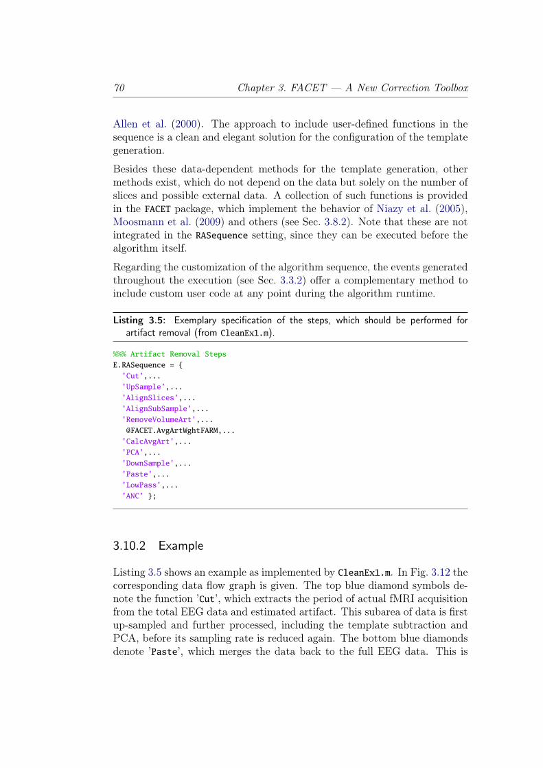
70 Chapter 3. FACET — A New Correction Toolbox
Allen et al. (2000). The approach to include user-defined functions in thesequence is a clean and elegant solution for the configuration of the templategeneration.
Besides these data-dependent methods for the template generation, othermethods exist, which do not depend on the data but solely on the number ofslices and possible external data. A collection of such functions is providedin the FACET package, which implement the behavior of Niazy et al. (2005),Moosmann et al. (2009) and others (see Sec. 3.8.2). Note that these are notintegrated in the RASequence setting, since they can be executed before thealgorithm itself.
Regarding the customization of the algorithm sequence, the events generatedthroughout the execution (see Sec. 3.3.2) offer a complementary method toinclude custom user code at any point during the algorithm runtime.
Listing 3.5: Exemplary specification of the steps, which should be performed forartifact removal (from CleanEx1.m).
%%% Artifact Removal StepsE.RASequence = ’Cut’,...’UpSample’,...’AlignSlices’,...’AlignSubSample’,...’RemoveVolumeArt’,[email protected],...’CalcAvgArt’,...’PCA’,...’DownSample’,...’Paste’,...’LowPass’,...’ANC’ ;
3.10.2 Example
Listing 3.5 shows an example as implemented by CleanEx1.m. In Fig. 3.12 thecorresponding data flow graph is given. The top blue diamond symbols de-note the function ’Cut’, which extracts the period of actual fMRI acquisitionfrom the total EEG data and estimated artifact. This subarea of data is firstup-sampled and further processed, including the template subtraction andPCA, before its sampling rate is reduced again. The bottom blue diamondsdenote ’Paste’, which merges the data back to the full EEG data. This is

3.10 Algorithm Sequence 71
EEG Data Artifact
Up-Sample
Align Slices
Align Sub-Sample
Volume Artifact
Template Generation
Template Subtraction
PCA
Down-Sample
Low Pass
ANC
Output
Figure 3.12: Artifact removal sequence as configured by Lst. 3.5.

72 Chapter 3. FACET — A New Correction Toolbox
finally filtered with a low-pass filter and corrected using adaptive noise can-cellation (ANC). Note that the (reconstructed) artifact signal (starting atthe top right red circle) is initially zero, i.e. no artifact at all. The data isreconstructed step by step during the artifact removal.
3.11 Evaluation Framework
As soon as the EEG data with gradient artifacts is improved by the artifactcorrection algorithm, the quality of the results should be assessed. For thispurpose, an evaluation framework was developed as part of the toolbox. Itprovides an extensive set of performance indicators as utilized by differentauthors (compare Sec. 2.4).
3.11.1 Software Design
The goal was to perform multiple evaluation algorithms on the output datafrom the artifact removal algorithms. These evaluation results should besaved and then presented to the user in several formats. One format is to printthe numbers with some descriptive text to the screen. Additionally, LATEXsource code for tables and diagrams should be emitted to be used in high-quality publications. From the user perspective, the evaluation algorithmshould provide extensive configurability, but should also be usable as a Matlabone-line command.
As integral part of the artifact correction toolbox, the evaluation frameworkis included in the Matlab package FACET. The same modern design paradigmof object oriented programming (Sommerville, 2004) as for the correctionalgorithm is used. The software design provides a separation of the
• execution of performance indicator algorithms, from the• storage of their results, and the• presentation of these results.
This is achieved by the object-oriented design as shown in Fig. 3.13. Thefunctionality is divided and realized by the classes.
Eval is the main class which holds all evaluation algorithms. It is instan-tiated with the original and the corrected EEG data (EEGLAB datastructure). The evaluation is performed by the method eval(). The

3.11 Evaluation Framework 73
Eval
EEG_Channels// parameters ...result: EvalResult// internal data ...
Eval(EEG_orig,EEG_Corr,...)eval()// evaluation methods ...
EvalResult
pkpkrms_residualrms_correctedsnr_residualfft_allenfft_niazy
EvalResult()
EvalResultContainer
EvalResultInputNameShortTitle
EvalResultContainer(EvalResult)
EvalPrint
Container[]
EvalPrint(EvalResultOrContainer)AddResult(EvalResultOrContainer)print(file)
EvalPrintText
EvalPrintText(EvalResult)print(file)
EvalPrintLaTeX
CmdPrefix
EvalPrintLaTeX(EvalResult)print(file)
Figure 3.13: UML Class Diagram of the evaluation framework.
results are stored in the member variable result, which is an instanceof the EvalResult class.
EvalResult is a storage object for the evaluation results.
EvalResultContainer wraps the EvalResult object and adds meta informa-tion (the variable name and a short title), later used by the EvalPrint
descendants.
EvalPrint is an abstract base class to print the evaluation results in an arbi-trary format. Actual printing routines are implemented in descendantclasses (see below).
EvalPrintText is a descendant class of EvalPrint which implements theprint() method to display a human-readable table.
EvalPrintLaTeX also descends from EvalPrint and implements the creationof output to be used in LATEX documents. It generates code using the

74 Chapter 3. FACET — A New Correction Toolbox
TikZ and PGFPlots packages with multiple commands, which are usedby the user inside of table and figure environments.
3.11.2 Data Preparation
All datasets contain recordings during which fMRI acquisition was performed.They additionally contain short periods before and after the fMRI acquisitionwhich don’t show gradient artifacts. To utilize these periods for comparisonwith the corrected data, the period before and after the fMRI acquisitionare merged to a single interval and supplied to the individual evaluationalgorithms.
A second point to consider is the processing of these periods by the artifactcorrection algorithms. In some cases, only the period during fMRI acquisitionis filtered by a low-pass (cmp. Sec. 3.9). In the left spectrogram in Fig. 3.11,the blue portions in the frequency range above 70Hz from approx. 30 s to150 s show, that the low-pass was only applied for this period. A comparisonof the corrected data (with an applied low-pass) with data outside of thefMRI gradient artifacts (without a low-pass filtering) would lead to invalidresults. Therefore the evaluation framework provides means to apply filtersto the undisturbed data.
3.11.3 Performance Indicators
Section 2.4 summarizes performance indicators found in publications. Manyof these were implemented in the evaluation framework. Unfortunately thepublications didn’t provide enough details for all algorithms, therefore someassumptions were necessary.
Median Imaging Artifact. The median signal amplitude range acrossall channels is calculated. The amplitude of the artifact is used by Allen etal. (2000) as an indicator of the quality of their algorithm (see Sec. 2.4.1).Unfortunately the publication is vague on the definition of this indicatortherefore some assumptions had to be made for the implementation.
Ten intervals with a length of 10% to 20% more than the slice period time aretaken from the EEG data of every channel. These intervals are equally spacedwith a distance to cover the whole duration of the fMRI acquisition. Therange (maximum value minus minimum value) of each interval is calculatedand averaged across the ten samples. This results in a mean imaging artifact

3.11 Evaluation Framework 75
range (also called peak-to-peak value) of every channel of every subject ofevery recording. Finally the minimum, maximum and median of these rangesare calculated, where the latter is called “Median Imaging Artifact”.
Although Allen et al. (2000) solely use the median imaging artifact to showthe reduction of the residual artifact, we also calculate the median range ofthe EEG data without fMRI acquisition for comparison. Therefore the verysame algorithm is performed on the (merged) EEG data before and afterfMRI acquisition.
RMS Corrected to Unimpaired. The performance indicator used byMoosmann et al. (2009) is the ratio of the RMS of the (DC-free) correctedEEG signal to the RMS of the signal without fMRI acquisition (see Sec. 2.4.2).The evaluation tool calculates this ratio individually for every channel andreturns descriptive statistics on them.
RMS Uncorrected to Corrected. van der Meer et al. (2010) use theratio of the RMS of the uncorrected EEG signal to the RMS of the correctedsignal (see Sec. 2.4.2). The evaluation tool calculates this ratio individuallyfor every channel and returns descriptive statistics on them.
SNR of Corrected. The Signal to Noise Ratio (SNR) as defined by equa-tion (2.4) in Sec. 2.4.3 relates the undistorted signal power S to the noisepower N . In many cases these values are not directly available for practicalcalculations. Examples are the EEG signal from an fMRI acquisition or theresult from the artifact correction algorithm.
In these cases only the power of the distorted signal D is known. Assumingadditive noise, the distorted signal can be written as sum of the undistortedsignal and the noise signal xD(t) = xS(t) + xN(t). Utilizing the statisticalindependence, the power of the undistorted signal and the noise signal arealso additive: D = S +N .
Most EEG datasets with fMRI acquisition also contain periods without fMRIacquisition. These can be used as a sample of the undistorted signal tocalculate S. With this information, the noise power is given by N = D − Sand the SNR is
SNR =S
D − S . (3.3)

76 Chapter 3. FACET — A New Correction Toolbox
This equation is applied for every channel of the corrected EEG dataset withD as the corrected signal and S the signal outside of the fMRI acquisitionperiods.
Due to the subtraction term D − S the result can be negative. This hap-pens when the correction algorithm has removed more signal power than theartifact signal power. Physically a negative noise power N = D − S doesnot make sense, therefore only positive SNR values are considered in thedescriptive statistics.
Median Residual Activity. To compare the activity in four EEG fre-quency bands (0.8–4Hz (Delta waves), 4–8Hz (Theta waves), 8–12Hz (Al-pha waves) and 12–24Hz (part of the Beta wave spectrum)) (Allen et al.,2000, see also Sec. 2.4.4), ten equally spaced periods of 3 sec. (which are 6.000samples at a sampling rate of 2 kSps) were averaged and then transformedto frequency domain with an FFT. The activity is calculated as the sum ofthe magnitude spectrum in the frequency band.
Power Density at Slice Frequency. This performance indicators liststhe power density reduction achieved by the artifact correction at the slicefrequency and its harmonics. For the given original and the corrected datasetsan FFT is performed for every channel. The magnitudes at the frequencybins of the volume and the slice frequencies and four harmonics are divided(corrected/original) and squared. These values are converted to decibel (dB)and the mean over all channels is calculated.
The automatic generation of LATEX source code by EvalPrintLaTeX for clarityonly includes a subset of the evaluation results. For the “Median ImagingArtifact” the median amplitude range of the corrected data is shown. The“RMS Corrected to Unimpaired”, the “RMS Uncorrected to Corrected” aswell as the “SNR of Corrected” are represented by the respective mean valuesacross all channels. The mean SNR value is supplemented by the number ofincluded values with a positive noise power. For the “Power Density at SliceFrequency” the averaged value in dB of the slice frequency and its harmonicsacross all channels are given.
3.11.4 Usage Examples
For a quick evaluation of the results, the evaluation framework is usable witha one line Matlab command. The example in Lst. 3.6 compares the corrected

3.11 Evaluation Framework 77
dataset clean1 to the raw dataset EEG_FMRIB, but limits the comparison tochannels 1 to 30 (because channel 31 contains ECG data, see Sec. 4.1.1).Additionally, the number of slices per volumes is given as 21. The command-line creates an Eval object and executes its eval() method. Then it createsan EvalPrintText object and print()s the evaluation result to the screen.The evaluation result is stored to the variable eval1.
Listing 3.6: Exemplary one-line Matlab command to evaluate the result of the correc-tion algorithm and to print the result.
>> eval1=FACET.EvalPrintText(FACET.Eval(EEG_FMRIB,cleaned1,[1:30],21).eval()).print();
For a more complex cases, it is advisable to store the Eval, EvalResult andEvalPrint* objects to variables and access their member variables for finetuning. An example is given in Lst. 3.7. In the first part, three datasetsare evaluated, each corrected with different algorithm parameters. In thesecond part, a EvalPrintLaTeX object is created. The evaluation resultsare added and short labels are provided. A prefix for the generated LATEXcommands is given, before the result is printed to a file. This can be used ina LATEX document, which flexibly places the generated tables and diagrams.Chapter 4 extensively uses this feature.
Listing 3.7: Example of the usage of the evaluation framework to generate LATEXtables and diagrams.
% Evaluate dataeval_CleanEx4 = FACET.Eval(EEG_FMRIB,HBM_CleanEx4,[1:30],21).eval();eval_Niazy = FACET.Eval(EEG_FMRIB,HBM_Niazy, [1:30],21).eval();eval_CleanEx1 = FACET.Eval(EEG_FMRIB,HBM_CleanEx1,[1:30],21).eval();% Create LaTeX include file with tables and diagramsepl=FACET.EvalPrintLaTeX();epl.AddResult(FACET.EvalResultContainer(eval_CleanEx4,’Allen’));epl.AddResult(FACET.EvalResultContainer(eval_Niazy, ’Niazy’));epl.AddResult(FACET.EvalResultContainer(eval_CleanEx1,’EEGfMRI’));epl.CmdPrefix=’HBM’;% Save to filefid=fopen(’../paper/eval.inc.tex’,’w’);epl.print(fid);fclose(fid);


4
Evaluation of EEGfMRI
THE presented artifact correction toolbox “FACET” is used to implementan optimum artifact correction algorithm named “EEGfMRI”. The de-
gree to which the artifacts were removed by this algorithm as well as selectedexisting algorithms as summarized in Sec. 2.3 is evaluated with the perfor-mance indicators outlined in Sec. 2.4. For the reproducible and user-friendlyapplication of the evaluation a dedicated framework was developed, whichwas described in Sec. 3.11. The results for the existing artifact correctionalgorithms and for the presented new algorithm are given in the followingsections. This is followed by a discussion of these results.
Two datasets are used for the evaluation: the example data supplied withthe FMRIB plugin by Niazy et al. (2005) and an own pilot dataset (seeSec. 4.1). These are corrected using the algorithm by Allen et al. (2000) (seeSec. 2.3.1) and the algorithm by Niazy et al. (2005) (see Sec. 2.3.2) as wellas with EEGfMRI. The abbreviations “Allen”, “Niazy” and “EEGfMRI” willbe used from now on.
79

80 Chapter 4. Evaluation of EEGfMRI
Precisely, the toolbox FACET is also used to implement the algorithm byAllen et al. (2000) showing its universal applicability. Allen et al. (2000)report to use blocks of 25 volumes for averaging if the fMRI sequence producesvolume gaps. Since the FMRIB dataset was recorded with only 40 volumesand the FACET toolbox inherently handles volume gaps, the algorithm issetup to treat the data as Allen et al. (2000) did if no volume gaps werepresent. This means that a block length of 100 slices are used. The pilotdataset does not show volume gaps, so this is also corrected with 100 slices perblocks. The equal treatment of both datasets also allows better comparisonof the results.
Since FACET is a generic toolbox of which multiple options and proceduresare used by EEGfMRI, the individual gain of each option is investigated.These options should provide an improvement to the starting point of thealgorithm by Niazy et al. (2005). According to the generalized scheme offMRI artifact correction algorithms (see Sec. 3.2.4) the evaluation is splitto the improvements located in the pre-processing, template-generation andpost-processing parts.
Firstly, the pre-processing and template generation improvements providedby FACET and employed by EEGfMRI are investigated. The post-processingsteps are disabled to enable a clear view to their effect. This evaluation ispreceded by a comparison of the three mentioned algorithms with deactivatedpost-processing. This is followed by the incremental activation of the pre-processing and template-generation steps.
Secondly, the post-processing steps also used by Niazy et al. (2005) are incre-mentally activated in EEGfMRI and the results evaluated. Finally all threealgorithms are compared with fully activated post-processing.
The same evaluation is then performed again using the pilot dataset. The fi-nal comparison is extended by the evaluation of the artifact correction resultsachieved by the online algorithm provided by the used EEG recorder.
All computations were performed using Matlab 7.8.0.347 (R2009a) 64-bit(glnxa64) on a GNU/Linux Debian operating system (kernel release 3.2,architecture x86_64). It was executed on a PC with an Intel R© CoreTM i7860 CPU with 2.80GHz and 8GiB RAM. Although a multi-core CPU wasused, only a single computational task was employed to work around a Matlabbug.1
1http://www.mathworks.com/support/bugreports/532399 [visited 2012-04-24, login re-quired], Matlab was started with the command line parameter -singleCompThread

4.1 Data 81
4.1 Data
For the evaluation two datasets are used, the FMRIB and an own pilotdataset. This section describes the datasets including their origin, propertiesand appearance.
4.1.1 FMRIB Dataset
The FMRIB dataset is included in the FMRIB EEGLAB plugin and isalso freely available at http://www.fmrib.ox.ac.uk/eeglab/fmribplugin/.The site doesn’t give a lot details on the recording, but those given are mostlyconsistent with Niazy et al. (2005). Therefore we use this paper for informa-tion which is missing for the dataset as well as results from the investigationof the dataset itself.
The MR device employed for acquisition was a 3T Varian Inova scanner.They used an echo planar imaging (EPI) sequence with TR=3 s and 21 slicesper volume with a slice time of 142.6ms and an inter-volume gap of 5ms.Each slice consists of 64 lines. A total of 40 volumes were recorded whichresults in an acquisition time of 120 s (2 minutes) and 840 slices. The subject’stask was to open and close his eyes every 10 seconds.
Of the total 32 recorded channels, 30 EEG channels according to the 10–20international system with common reference electrode at the FCz locationwere used. These are complemented by two bipolar channels for electromyo-graph (EMG) and electrocardiograph (ECG). An SystemPLUS EEG systemand an SD32 MRI amplifier by Micromed s.r.l., TV, Italy were employed.All channels had a 10 kΩ series resistor for current limiting and a 600Hz,first order (20 dB/decade) low-pass anti-aliasing filter as well as a 0.15Hz,second-order (40 dB/decade) high-pass filter. The recording used a sigma-delta analog-to-digital converter (ADC) with a sampling rate of 2048Hz. Theamplifier has an input voltage range of ±25.6mV and a resolution of 12.2 nVwhat means 22 bits resolution.
The data itself ranges from −45.5mV to +51.8mV. Visual inspection revealsno clipping or saturation effects. It has a quantization resolution of 390.2 nV,so it seems that it used a different amplifier setting with a 32 times (5 bits)coarser resolution and also higher input voltage range.
The EEG was recorded for 162 s and stored as Matlab file with data typesingle (IEEE Task P754, 1985) (32 bits, 23 bits mantissa, 8 bits exponent).

82 Chapter 4. Evaluation of EEGfMRI
Since the dynamic range of the data is approx. 18 bits, and the single precisiondata type offers 23 bits mantissa, it does not affect the data resolution.
This dataset was used throughout this work to visualize the artifact, seeFigs. 1.1, 2.2, 2.3 and 2.5 for reference on the amplitude values and artifactpattern.
4.1.2 Pilot Dataset
The pilot dataset was recorded for this work as a test acquisition at theMR Center of Excellence, Medical University Vienna, Vienna, Austria inaccordance with the 1975 Helsinki declaration and local ethics regulations.The subject’s task was to keep his eyes closed, stay as still as possible andnot thinking of anything.
The MR acquisition was performed with a 3T Siemens TIM Trio scannerusing a 32-channel head coil. The parameters of the echo planar imaging(EPI) sequence were a volume repetition time of TR=2 s with 25 axial slicesper volume and a slice time of 80ms (12.5Hz). The sequence does not havean inter-volume gap. Each slice consists of a 128×128 matrix. A total of 150volumes were recorded which results in 5 minutes of acquisition.
For the EEG and EMG recording a neuroConn NEURO PRAX R© MR devicewith 64 channels, an 800Hz anti-aliasing filter, with a 24 bit ADC was used(neuroConn NEURO PRAX MR, 2009; Schlegelmilch et al., 2004; Berkes,Schellhorn, Schlegelmilch, Markert, & Husar, 2004; Berkes, Husar, et al.,2004). The data was recorded with 2000 samples per second.
The dataset consists of 22 channels of which three channels are EEG (Fz, Cz,Pz) and ten channels are unipolar EMG signals from which 5 bipolar EMGchannels are calculated. These measured the facial muscles M. frontalis,M. corrugator supercilii, M. orbicularis oculi, M. zygomaticus major, andM. masseter. Two channels recorded the horizontal and vertical electroocu-logram (EOG), one channel recorded the current heart rate and one recordedthe electrocardiograph (ECG). The latter does not contain data due to arecording problem.
The ten raw unipolar EMG channels have a range from−263.4mV to 286.4mV,the five bipolar EMG channels range from −251.4mV to 342.2mV. The twoEOG channels range from −213.0mV to 508.9mV. The three EEG channelsrange from −156.0mV to 503.8mV. The data does not show quantizationeffects so it seems it was preprocessed and no conclusions on the ADC reso-

4.2 Comparison Without Post-Processing 83
lution can be drawn. Figure 4.1 shows an exemplary section of the datasetrecorded at an EMG electrode.
The EEG and EMG data was recorded for 324.5 s and stored as a Matlabfile with data type single.
0 50 100 150 200 250 300
−250
−200
−150
−100
−50
0
t / ms
U/
mV
Figure 4.1: Exemplary section of the pilot dataset with four consecutive fMRI sliceacquisition periods measured with a facial EMG electrode. The artifact amplitudeis nearly 300mV.
4.2 Comparison Without Post-Processing
As a starting point, the results of the algorithms of Allen et al. (2000),Niazy et al. (2005) and EEGfMRI are compared, while the post-processingis switched off. EEGfMRI is configured with all improvements over Niazy etal. (2005) switched off, i.e. to be as close as possible to their algorithm. Theevaluation results are given in Tab. 4.1 and Figs. 4.2 to 4.7. For a descriptionof the utilized performance indicators see Sec. 3.11.3.
All three algorithms show similar results. Allen shows slightly less residualmedian imaging artifact and RMS of the corrected signal and hence higherratio of RMS of the uncorrected to the corrected signal and higher SNR. Themedian residual activity is worse for the 8–12Hz and 12–24Hz bands butbetter for the 0.8–4Hz and 4–8Hz bands.
The reason for this advantage most probably lies in Allen’s template genera-tion algorithm. As outlined in Sec. 2.3.1 the main problem of averaging slices

84 Chapter 4. Evaluation of EEGfMRI
Table 4.1: Comparison of the results of Allen et al. (2000), Niazy et al. (2005) andEEGfMRI without post-processing.
Allen Niazy EEGfMRIMedian Imaging Artifact (µV) 513 557 557RMS Corrected to Unimpaired 4.92 5.67 5.68RMS Uncorrected to Corrected 20.3 17.9 17.9SNR of Corrected 0.224 (30) 0.218 (30) 0.215 (30)Median Residual Activity
0.8 – 4.0Hz4.0 – 8.0Hz8.0 – 12.0Hz12.0 – 24.0Hz
30% 35% 35%20% 25% 25%35% 25% 25%33% 26% 25%
Power Density at Slice Frequency1: 7.00Hz2: 14.00Hz3: 21.00Hz4: 28.00Hz5: 35.00Hz
-53 dB -50 dB -49 dB-50 dB -52 dB -48 dB-63 dB -62 dB -58 dB-59 dB -59 dB -55 dB-64 dB -62 dB -57 dB
is the missing synchronization of the fMRI and EEG periods which leads toa sub-sample uncertainty. The algorithm selects slices for averaging with across-correlation of at least 0.975 (cmp. Sec. 2.3.1) while the others do notconsider the congruence.
EEGfMRI shows nearly identical values to Niazy except for the power densityreduction at slice frequency harmonics, where it is 4–5 dB worse.

4.2 Comparison Without Post-Processing 85
Allen Niazy EEGfMRI0
200
400
600
513557 557
Med
ian
pk-p
k/µV
Figure 4.2: Comparison of the results of Allen et al. (2000), Niazy et al. (2005) andEEGfMRI without post-processing by the median imaging artifact (lower is better).
Allen Niazy EEGfMRI0
2
4
6
4.92
5.67 5.68
RM
SC
orre
cted
toU
nim
pair
ed
Figure 4.3: Comparison of the results of Allen et al. (2000), Niazy et al. (2005) andEEGfMRI without post-processing by the RMS of the corrected to the unimpairedsignal (nearer to 1.0 is better).

86 Chapter 4. Evaluation of EEGfMRI
Allen Niazy EEGfMRI0
5
10
15
2020.3
17.9 17.9
RM
SU
ncor
rect
edto
Cor
rect
ed
Figure 4.4: Comparison of the results of Allen et al. (2000), Niazy et al. (2005) andEEGfMRI without post-processing by the RMS of the uncorrected to the correctedsignal (larger is better).
Allen Niazy EEGfMRI0.00
0.05
0.10
0.15
0.20
0.224 0.218 0.215
SNR
ofC
orre
cted
Figure 4.5: Comparison of the results of Allen et al. (2000), Niazy et al. (2005)and EEGfMRI without post-processing by the SNR of the corrected signal (larger isbetter).

4.2 Comparison Without Post-Processing 87
0.8–4Hz 4–8Hz 8–12Hz 12–24Hz0
10
20
3030
20
3533
35
25 25 26
35
25 25 25
MedianResidua
lActivity
/%
AllenNiazyEEGfMRI
Figure 4.6: Comparison of the results of Allen et al. (2000), Niazy et al. (2005) andEEGfMRI without post-processing by the median residual activity (lower is better).
7Hz 14Hz 21Hz 28Hz 35Hz0
20
40
6053 50
6359
64
50 52
62 59 62
49 48
5855 57
Pow
erD
ensi
tyR
educ
tion
/dB
AllenNiazyEEGfMRI
Figure 4.7: Comparison of the results of Allen et al. (2000), Niazy et al. (2005) andEEGfMRI without post-processing by the power density reduction at slice frequencyharmonics (larger is better).

88 Chapter 4. Evaluation of EEGfMRI
4.3 Incremental Activation of Pre-Processing and Tem-plate Generation Improvements
In this section six improvements of the pre-processing and template gener-ation steps are added incrementally to the correction algorithm. The orderof activation is the same as as the order of their occurrence in the algorithmflow (cmp. Sec. 3.10 and Fig. 3.12).
The starting point (abbreviated raw) are the settings used in the previoussection. To be as similar to Niazy et al. (2005) as possible, firstly the cut-offfrequency during upsampling was set to 1.0 which results in interpolationerrors (see Sec. 3.6.3). Secondly, the template generation used alternatingslices, i.e., slices 2, 4, 6, ... for the first slice, slices 3, 5, 7, ... for the secondslice, and so on, using a sliding average. And thirdly, the volume gaps in thetemplates were set to 0.0.
In the following abbreviations are used to specify each improvement through-out this section.
PreFilter adds a 1Hz high-pass to filter the EEG signal before any furtherprocessing (see Sec. 3.5).
Upsample0.5 corrects the interpolation cut-off frequency setting from 1.0to 0.5 (see Sec. 3.6.3).
AlignSubSample switches on the temporal alignment of the slices with sub-sample resolution to the reference slice (see Sec. 3.6).
RemoveVolumeArtifact removes the volume artifact at volume acquisitionboundaries (see Sec. 3.7).
AvgArtWghtFARM changes the template generation algorithm to select thebest fit slices for the averaging according to van der Meer et al. (2010)(see Sec. 3.8.2).
InterpolateVolGaps generates an interpolated signal during volume gapswhen calculating the artifact estimation instead of 0.0 as described atthe end of Sec. 3.8.1.
The results are given in Tab. 4.2 and Figs. 4.8 to 4.13.
(a) raw: The first column repeats the results from the previous section asreference.

4.3 Pre-Processing and Template Generation Improvements 89
Tab
le4.
2:Com
parison
oftheresults
with
increm
entala
ctivationof
thepre-processing
andtemplategeneratio
nim
provem
ents.
(a)raw
(b)+PreFilte
r(c)+Upsam
ple0.5
(d)+AlignS
ubSa
mple
(e)+Rem
oveVolum
eArt
(f)+AvgArtWgh
tFARM
(g)+InterpolateVolGaps
(a)
(b)
(c)
(d)
(e)
(f)
(g)
MedianIm
agingArtifa
ct(µ
V)
557
557
509
143
141
110
110
RMSCorrected
toUnimpa
ired
5.68
5.67
4.99
1.58
1.57
1.02
1.01
RMSUncorrected
toCorrected
17.9
18.0
20.1
64.6
65.2
93.5
93.6
SNR
ofCorrected
0.21
5(30)
0.22
5(30)
0.26
7(30)
2.61
(19)
3.51
(19)
4.29
(12)
4.36
(12)
MedianResidua
lActivity
0.8–
4.0Hz
4.0–
8.0Hz
8.0–12
.0Hz
12.0
–24
.0Hz
35%
37%
33%
33%
37%
47%
47%
25%
26%
24%
24%
27%
17%
15%
25%
25%
32%
31%
37%
37%
38%
25%
24%
30%
30%
27%
24%
22%
Pow
erDensity
atSliceFrequency
1:7.00
Hz
2:14
.00Hz
3:21
.00Hz
4:28
.00Hz
5:35
.00Hz
-49dB
-49dB
-51dB
-51dB
-49dB
-40dB
-39dB
-48dB
-48dB
-50dB
-50dB
-52dB
-47dB
-51dB
-58dB
-58dB
-62dB
-62dB
-62dB
-55dB
-57dB
-55dB
-55dB
-57dB
-56dB
-57dB
-54dB
-56dB
-57dB
-57dB
-60dB
-60dB
-61dB
-57dB
-61dB

90 Chapter 4. Evaluation of EEGfMRI
(b) +PreFilter: Adding a 1Hz high-pass pre-filter has only minor influence.
(c) +Upsample0.5: Correcting the interpolation error shows an improvementin all numbers except in the median residual activity from 8–24Hz.
(d) +AlignSubSample: If the slices are aligned with sub-sample resolution, alarge improvement in all time-domain values (median imaging artifact, RMScorrected to unimpaired, RMS uncorrected to corrected and SNR of cor-rected) is achieved. The frequency domain performance indicators (medianresidual activity and power density reduction at slice frequency) show mixedresults.
(e) +RemoveVolumeArt: Removing the volume artifact shows only a smallimprovement. The median residual activity from 0.8–12Hz even gets worseand the removed power density at slice frequency 7Hz also drops.
(f) +AvgArtWghtFARM: Using best-fit slices for averaging leads to a strongreduction of artifacts, as shown by the time-domain values. The frequencydomain shows increased residual activity at 0.8–4Hz and less removed powerdensity at slice frequency harmonics.
(g) +InterpolateVolGaps: Ensuring a continuous signal during volume gapswith a linear interpolated signal has a small positive effect.
A closer look at the FFT of the corrected EEG signal shows that (a)-(e)have deep notches at the slice frequency and its harmonics. These result in agood power density reduction at these frequencies. When AvgArtWghtFARMis added, these notches vanish and show a continuous spectrum. This meansthat less of the real EEG components are removed.
In total, these six improvements result in a reduction of the median imagingartifact and the RMS of the corrected to the RMS of the unimpaired signalby a factor of approximately 5 while the RMS of the uncorrected to the RMSof the corrected signal increases by approximately the same amount. TheSNR is even improved by a factor of 20.

4.3 Pre-Processing and Template Generation Improvements 91
(a) (b) (c) (d) (e) (f) (g)0
200
400
600 557 557509
143 141110 110M
edia
npk
-pk
/µV
Figure 4.8: Comparison of the results with incremental activation of the pre-processingand template generation improvements by the median imaging artifact (lower is bet-ter). (a) raw, (b) +PreFilter, (c) +Upsample0.5, (d) +AlignSubSample, (e) +Re-moveVolumeArt, (f) +AvgArtWghtFARM, (g) +InterpolateVolGaps
(a) (b) (c) (d) (e) (f) (g)0
2
4
6 5.68 5.674.99
1.58 1.571.02 1.01
RM
SC
orre
cted
toU
nim
pair
ed
Figure 4.9: Comparison of the results with incremental activation of the pre-processingand template generation improvements by the RMS of the corrected to the unim-paired signal (nearer to 1.0 is better). (a) raw, (b) +PreFilter, (c) +Upsample0.5,(d) +AlignSubSample, (e) +RemoveVolumeArt, (f) +AvgArtWghtFARM, (g) +In-terpolateVolGaps

92 Chapter 4. Evaluation of EEGfMRI
(a) (b) (c) (d) (e) (f) (g)0
20
40
60
80
100
17.9 18.0 20.1
64.6 65.2
93.5 93.6R
MS
Unc
orre
cted
toC
orre
cted
Figure 4.10: Comparison of the results with incremental activation of the pre-processing and template generation improvements by the RMS of the uncorrectedto the corrected signal (larger is better). (a) raw, (b) +PreFilter, (c) +Upsam-ple0.5, (d) +AlignSubSample, (e) +RemoveVolumeArt, (f) +AvgArtWghtFARM,(g) +InterpolateVolGaps
(a) (b) (c) (d) (e) (f) (g)0
1
2
3
4
0.215 0.225 0.267
2.61
3.51
4.29 4.36
SNR
ofC
orre
cted
Figure 4.11: Comparison of the results with incremental activation of the pre-processing and template generation improvements by the SNR of the corrected signal(larger is better). (a) raw, (b) +PreFilter, (c) +Upsample0.5, (d) +AlignSubSam-ple, (e) +RemoveVolumeArt, (f) +AvgArtWghtFARM, (g) +InterpolateVolGaps

4.3 Pre-Processing and Template Generation Improvements 93
0.8–4Hz
4–8Hz
8–12
Hz
12–24Hz
0
1020304050
35
2525
25
37
2625
24
33
24
3230
33
24
3130
37
27
37
27
47
17
37
24
47
15
38
22
MedianResidualActivity/%
(a)
(b)
(c)
(d)
(e)
(f)
(g)
Fig
ure
4.12
:Com
parison
oftheresults
with
increm
entala
ctivationof
thepre-processing
andtemplategeneratio
nim
provem
ents
bythemedianresidu
alactiv
ity(low
erisbetter).
(a)raw,(b)+PreFilte
r,(c)+Upsam
ple0.5,(d)+AlignS
ubSa
mple,
(e)+Re-
moveVolum
eArt,(f)
+AvgArtWgh
tFARM,(g)
+InterpolateVolGaps

94 Chapter 4. Evaluation of EEGfMRI
7H
z14
Hz
21H
z28
Hz
35H
z0
20 40 60
4948
5855
57
4948
5855
57
5150
6257
60
5150
6256
60
4952
6257
61
40
47
5554
57
39
5157
5661
Power Density Reduction / dB
(a)(b)
(c)(d)
(e)(f)
(g)
Figure
4.13:Com
parisonof
theresults
with
incrementalactivation
ofthe
pre-processingand
template
generationim
provements
bythe
power
densityreduction
atslice
frequencyharm
onics(larger
isbetter).
(a)raw
,(b)
+PreFilter,
(c)+Upsam
ple0.5,(d)
+AlignSubSam
ple,(e)+Rem
oveVolum
eArt,(f)
+AvgA
rtWghtFA
RM,(g)
+InterpolateV
olGaps

4.4 Incremental Activation of Post-Processing Steps 95
4.4 Incremental Activation of Post-Processing Steps
In the previous sections the results of the pre-processing and template gener-ation with switched off post-processing were investigated. In this section thepost-processing steps are enabled incrementally. The following abbreviationsare used.
PCA adds a principal component analysis and removes the strongest com-ponents related to the fMRI artifact. This was called optimum basisset by Niazy et al. (2005).
LowPass filters the corrected signal with a 70Hz low-pass which removes allresidual high-frequency components. Compare the spectrogram givenin Fig. 3.11.
ANC uses adaptive noise cancellation as introduced by Allen et al. (2000)and also used by Niazy et al. (2005) (see Sec. 2.3.1 and 2.3.2).
These three post-processing steps are the same as used by Niazy et al. (2005).The results are given in Tab. 4.3 and Figs. 4.14 to 4.19.
(a) previous: Again, the last result of the previous section with all pre-processing and template generation improvements enabled is repeated forreference.
(b) PCA: Adding PCA shows a large improvement of the SNR and a small im-provement in the other time-domain performance indicators. The frequencydomain values do not change.
(c) LowPass: Filtering with a low-pass results in a strong reduction of themedian imaging artifact, i.e, the amplitude. The other time-domain perfor-mance indicators also show improvements. While the power density at slicefrequency harmonics did not change, the median residual activity is slightlydeteriorated in the 4–8Hz and 8–12Hz bands.
(d) ANC: A strong improvement of the median imaging artifact (amplitude)and the SNR are achieved using ANC. It also effects a considerable reductionof the power density in higher harmonics of the slice frequency (21Hz, 28Hzand 35Hz).
Note that the ratio of the RMS of the corrected EEG to the RMS of theunimpaired EEG is below 1.0. This means that the correction algorithm haseven removed a small fraction of the real EEG.

96 Chapter 4. Evaluation of EEGfMRI
Table 4.3: Comparison of the results with incremental activation of the post-processingsteps.(a) previous(b) +PCA(c) +LowPass(d) +ANC
(a) (b) (c) (d)Median Imaging Artifact (µV) 110 103 60.0 54.8RMS Corrected to Unimpaired 1.01 0.982 0.861 0.840RMS Uncorrected to Corrected 93.6 96.3 106 109SNR of Corrected 4.36 (12) 15.2 (12) 16.4 (8) 53.5 (6)Median Residual Activity
0.8 – 4.0Hz4.0 – 8.0Hz8.0 – 12.0Hz12.0 – 24.0Hz
47% 47% 43% 42%15% 15% 16% 13%38% 38% 42% 42%22% 22% 19% 10%
Power Density at Slice Frequency1: 7.00Hz2: 14.00Hz3: 21.00Hz4: 28.00Hz5: 35.00Hz
-39 dB -39 dB -39 dB -42 dB-51 dB -51 dB -51 dB -53 dB-57 dB -57 dB -57 dB -69 dB-56 dB -56 dB -57 dB -68 dB-61 dB -61 dB -61 dB -69 dB
(a) (b) (c) (d)0
20
40
60
80
100
120 110103
60.0 54.8
Med
ian
pk-p
k/µV
Figure 4.14: Comparison of the results with incremental activation of the post-processing steps by the median imaging artifact (lower is better). (a) previous,(b) +PCA, (c) +LowPass, (d) +ANC

4.4 Incremental Activation of Post-Processing Steps 97
(a) (b) (c) (d)0
0.2
0.4
0.6
0.8
11.01 0.982
0.861 0.840R
MS
Cor
rect
edto
Uni
mpa
ired
Figure 4.15: Comparison of the results with incremental activation of the post-processing steps by the RMS of the corrected to the unimpaired signal (nearerto 1.0 is better). (a) previous, (b) +PCA, (c) +LowPass, (d) +ANC
(a) (b) (c) (d)0
20
40
60
80
100
120
93.6 96.3106 109
RM
SU
ncor
rect
edto
Cor
rect
ed
Figure 4.16: Comparison of the results with incremental activation of the post-processing steps by the RMS of the uncorrected to the corrected signal (largeris better). (a) previous, (b) +PCA, (c) +LowPass, (d) +ANC

98 Chapter 4. Evaluation of EEGfMRI
(a) (b) (c) (d)0
10
20
30
40
50
4.36
15.2 16.4
53.5
SNR
ofC
orre
cted
Figure 4.17: Comparison of the results with incremental activation of the post-processing steps by the SNR of the corrected signal (larger is better). (a) previous,(b) +PCA, (c) +LowPass, (d) +ANC
0.8–4Hz 4–8Hz 8–12Hz 12–24Hz0
10
20
30
40
50 47
15
38
22
47
15
38
22
43
16
42
19
42
13
42
10
MedianResidua
lActivity/%
(a)(b)(c)(d)
Figure 4.18: Comparison of the results with incremental activation of the post-processing steps by the median residual activity (lower is better). (a) previous,(b) +PCA, (c) +LowPass, (d) +ANC

4.4 Incremental Activation of Post-Processing Steps 99
7 Hz 14 Hz 21 Hz 28 Hz 35 Hz0
20
40
60
39
5157 56
61
39
5157 56
61
39
5157 57
61
42
53
69 68 69
Pow
erD
ensi
tyR
educ
tion
/dB
(a)(b)(c)(d)
Figure 4.19: Comparison of the results with incremental activation of the post-processing steps by the power density reduction at slice frequency harmonics (largeris better). (a) previous, (b) +PCA, (c) +LowPass, (d) +ANC

100 Chapter 4. Evaluation of EEGfMRI
4.5 Comparison with Post-Processing
Finally, all pre-processing and template generation improvements and allpost-processing options are used in EEGfMRI and compared with Allen etal. (2000) and Niazy et al. (2005). Note that Allen et al. (2000) does not usePCA in post-processing. Although their low-pass filter has a cut-off frequencyof 80Hz, here it is set to 70Hz as used by Niazy et al. (2005) and EEGfMRI.An exemplary section of the EEG signal as result of the EEGfMRI algorithmis shown in Fig. 4.20. The results are given in Tab. 4.4 and Figs. 4.21 to 4.26.
0 0.5 1 1.5 2 2.5 3 3.5 4 4.5 5 5.5−50
−40
−30
−20
−10
0
10
20
30
40
t / s
U/µV
Figure 4.20: Exemplary section of the FMRIB dataset (see Sec. 4.1.1) after artifactremoval with the EEGfMRI algorithm. The signal does not show any slice or volumeartifacts. The residual variation is due to the BCG artifact which is not consideredin this work.
All performance indicators in time-domain (median imaging artifact, RMS,SNR) show an advantage of Niazy over Allen as well as a strong improvementof EEGfMRI over both.
On the other hand, the frequency domain performance indicators show apartial deterioration in the 0.8–4Hz and 8–12Hz bands of the median residualactivity. While these bands do not contain slice frequency harmonics (7Hz,14Hz, 21Hz, 28Hz, ...), these are present in the 4–8Hz and 12–24Hz bands,which both show a noticeable improvement over Niazy.
The power density reduction at slice frequency harmonics shows a deteriora-tion at 7Hz and 14Hz compared to Niazy and similar results for the higherharmonics. The reason is the same as already discussed in Sec. 4.3 that

4.5 Comparison with Post-Processing 101
Table 4.4: Comparison of the results of Allen et al. (2000), Niazy et al. (2005) andEEGfMRI with post-processing.
Allen Niazy EEGfMRIMedian Imaging Artifact (µV) 71.0 64.9 54.8RMS Corrected to Unimpaired 0.979 0.922 0.840RMS Uncorrected to Corrected 93.7 99.6 109SNR of Corrected 4.17 (11) 11.9 (9) 53.5 (6)Median Residual Activity
0.8 – 4.0Hz4.0 – 8.0Hz8.0 – 12.0Hz12.0 – 24.0Hz
28% 29% 42%15% 20% 13%45% 33% 42%25% 23% 10%
Power Density at Slice Frequency1: 7.00Hz2: 14.00Hz3: 21.00Hz4: 28.00Hz5: 35.00Hz
-52 dB -52 dB -42 dB-56 dB -57 dB -53 dB-68 dB -68 dB -69 dB-69 dB -70 dB -68 dB-67 dB -68 dB -69 dB
EEGfMRI spectrum does not show deep notches at slice frequency harmon-ics but an even form.

102 Chapter 4. Evaluation of EEGfMRI
Allen Niazy EEGfMRI0
20
40
60
71.064.9
54.8M
edia
npk
-pk
/µV
Figure 4.21: Comparison of the results of Allen et al. (2000), Niazy et al. (2005) andEEGfMRI with post-processing by the median imaging artifact (lower is better).
Allen Niazy EEGfMRI0
0.2
0.4
0.6
0.8
1 0.9790.922
0.840
RM
SC
orre
cted
toU
nim
pair
ed
Figure 4.22: Comparison of the results of Allen et al. (2000), Niazy et al. (2005)and EEGfMRI with post-processing by the RMS of the corrected to the unimpairedsignal (nearer to 1.0 is better).

4.5 Comparison with Post-Processing 103
Allen Niazy EEGfMRI0
20
40
60
80
100
120
93.799.6
109R
MS
Unc
orre
cted
toC
orre
cted
Figure 4.23: Comparison of the results of Allen et al. (2000), Niazy et al. (2005)and EEGfMRI with post-processing by the RMS of the uncorrected to the correctedsignal (larger is better).
Allen Niazy EEGfMRI0
10
20
30
40
50
4.17
11.9
53.5
SNR
ofC
orre
cted
Figure 4.24: Comparison of the results of Allen et al. (2000), Niazy et al. (2005) andEEGfMRI with post-processing by the SNR of the corrected signal (larger is better).

104 Chapter 4. Evaluation of EEGfMRI
0.8–4Hz 4–8Hz 8–12Hz 12–24Hz0
10
20
30
40
28
15
45
2529
20
33
23
42
13
42
10
MedianResidua
lActivity
/%
Allen Niazy EEGfMRI
Figure 4.25: Comparison of the results of Allen et al. (2000), Niazy et al. (2005) andEEGfMRI with post-processing by the median residual activity (lower is better).
7Hz 14Hz 21Hz 28Hz 35Hz0
20
40
6052
56
68 69 67
5257
68 70 68
42
53
69 68 69
Pow
erD
ensi
tyR
educ
tion
/dB
AllenNiazyEEGfMRI
Figure 4.26: Comparison of the results of Allen et al. (2000), Niazy et al. (2005) andEEGfMRI with post-processing by the power density reduction at slice frequencyharmonics (larger is better).

4.6 Pilot Dataset 105
4.6 Pilot Dataset
In this section the same evaluation is performed with the pilot dataset. Thefinal comparison with all pre-processing and template-generation improve-ments and all post-processing steps enabled is extended by the evaluationof the resulting EEG data from the built-in algorithm of the neuroConnNEURO PRAX R© MR EEG recorder (see Sec. 4.1.2).
The artifact amplitude of the pilot dataset is much larger than the amplitudeof the FMRIB dataset (see Tab. 2.1, Sec. 4.1.2 and Fig. 4.1). While theFMRIB dataset has a median range of 17.9mVpp the pilot dataset has anearly 23 times larger range of 408.8mVpp.
4.6.1 Comparison Without Post-Processing
As first step the results of the algorithms by Allen et al. (2000), Niazy et al.(2005) and the presented algorithm EEGfMRI are compared with disabledpost-processing. The results are shown in Tab. 4.5 and Figs. 4.27 to 4.32.
Table 4.5: Comparison of the results of Allen et al. (2000), Niazy et al. (2005) andEEGfMRI without post-processing.
Allen Niazy EEGfMRIMedian Imaging Artifact (µV) 10533 9465 11367RMS Corrected to Unimpaired 29.4 26.6 28.0RMS Uncorrected to Corrected 40.8 45.2 42.8SNR of Corrected 0.00591 (20) 0.00705 (20) 0.00653 (20)Median Residual Activity
0.8 – 4.0Hz4.0 – 8.0Hz8.0 – 12.0Hz12.0 – 24.0Hz
192% 142% 142%738% 665% 677%
1331% 1146% 1132%2934% 2830% 2920%
Power Density at Slice Frequency1: 12.50Hz2: 25.00Hz3: 37.50Hz4: 50.00Hz5: 62.50Hz
-62 dB -69 dB -69 dB-55 dB -61 dB -59 dB-54 dB -63 dB -59 dB-53 dB -63 dB -57 dB-51 dB -63 dB -56 dB
Niazy shows better results than Allen in all performance indicators. AlthoughEEGfMRI was configured as close as possible to Niazy, it shows slightly worseresults than Niazy.

106 Chapter 4. Evaluation of EEGfMRI
Allen Niazy EEGfMRI0
2,000
4,000
6,000
8,000
10,000
12,00010533
9465
11367
Med
ian
pk-p
k/µV
Figure 4.27: Comparison of the results of Allen et al. (2000), Niazy et al. (2005) andEEGfMRI without post-processing by the median imaging artifact (lower is better).
Allen Niazy EEGfMRI0
10
20
30 29.426.6 28.0
RM
SC
orre
cted
toU
nim
pair
ed
Figure 4.28: Comparison of the results of Allen et al. (2000), Niazy et al. (2005) andEEGfMRI without post-processing by the RMS of the corrected to the unimpairedsignal (nearer to 1.0 is better).

4.6 Pilot Dataset 107
Allen Niazy EEGfMRI0
10
20
30
4040.8
45.242.8
RM
SU
ncor
rect
edto
Cor
rect
ed
Figure 4.29: Comparison of the results of Allen et al. (2000), Niazy et al. (2005) andEEGfMRI without post-processing by the RMS of the uncorrected to the correctedsignal (larger is better).
Allen Niazy EEGfMRI0
0.002
0.004
0.006 0.00591
0.007050.00653
SNR
ofC
orre
cted
Figure 4.30: Comparison of the results of Allen et al. (2000), Niazy et al. (2005) andEEGfMRI without post-processing using the SNR of the corrected signal (larger isbetter).

108 Chapter 4. Evaluation of EEGfMRI
0.8–4Hz 4–8Hz 8–12Hz 12–24Hz0
1,000
2,000
3,000
192
738
1331
2934
142
665
1146
2830
142
677
1132
2920
MedianResidua
lActivity
/% Allen
NiazyEEGfMRI
Figure 4.31: Comparison of the results of Allen et al. (2000), Niazy et al. (2005) andEEGfMRI without post-processing using median residual activity (lower is better).
12.5Hz 25.0Hz 37.5Hz 50.0Hz 62.5Hz0
20
40
6062
55 54 53 51
69
61 63 63 6369
59 59 57 56
Pow
erD
ensi
tyR
educ
tion
/dB
AllenNiazyEEGfMRI
Figure 4.32: Comparison of the results of Allen et al. (2000), Niazy et al. (2005)and EEGfMRI without post-processing using the power density reduction at slicefrequency harmonics (larger is better).

4.6 Pilot Dataset 109
4.6.2 Incremental Activation of Pre-Processing and Template Gen-eration Improvements
In the next step the pre-processing and template generation improvementsare enabled incrementally for the EEGfMRI algorithm. The same abbre-viations as in Sec. 4.3 are used. Note that the MR sequence used for thepilot dataset does not employ volume gaps, therefore the option Interpolat-eVolGaps is not considered. On the other hand, the data does show volumeartifacts, thus the option RemoveVolumeArt is evaluated.
(a) raw: The results from the previous step are repeated as reference.
(b) +PreFilter: Using a 1Hz high-pass pre-filter deteriorates the results ac-cording to the time-domain data. The median residual activity shows slightimprovement. The power density reduction at slice frequency harmonicsshows large deterioration by as much as 10 dB.
(c) +Upsample0.5: Correcting the interpolation error shows an improvementin most numbers back to a level without the pre-filter. Switching off the pre-filter for this and the next steps has ambiguous effects, but generally doesnot give better results.
(d) +AlignSubSample: The alignment of all slice period to a reference periodwith sub-sample resolution shows a large improvement in all time-domainvalues. In contrast, the median residual activity slightly deteriorates in the 4–8Hz band. On the other hand, the power density reduction at slice frequencyharmonics is much improved.
(e) +RemoveVolumeArt: Removing the volume artifact shows an improve-ment in all values.
(f) +AvgArtWghtFARM: Using best-fit slices for averaging again leads to astrong reduction of the artifacts as shown by the time-domain values. Thefrequency domain performance indicator “median residual activity” showsa large improvement while the power density reduction at slice frequencyharmonics show a large deterioration.

110 Chapter 4. Evaluation of EEGfMRI
(a) (b) (c) (d) (e) (f)0
5,000
10,000
15,000
11367
14955
11983
6998 6726
1471
Med
ian
pk-p
k/µV
Figure 4.33: Comparison of the results with incremental activation of the pre-processing and template generation improvements by the median imaging artifact(lower is better). (a) raw, (b) +PreFilter, (c) +Upsample0.5, (d) +AlignSubSample,(e) +RemoveVolumeArt, (f) +AvgArtWghtFARM
(a) (b) (c) (d) (e) (f)0
10
20
30 28.0
32.728.9
20.4 19.5
5.38
RM
SC
orre
cted
toU
nim
pair
ed
Figure 4.34: Comparison of the results with incremental activation of the pre-processing and template generation improvements by the RMS of the corrected tothe unimpaired signal (nearer to 1.0 is better). (a) raw, (b) +PreFilter, (c) +Upsam-ple0.5, (d) +AlignSubSample, (e) +RemoveVolumeArt, (f) +AvgArtWghtFARM

4.6 Pilot Dataset 111
Tab
le4.
6:Com
parison
oftheresults
with
increm
entala
ctivationof
thepre-processing
andtemplategeneratio
nim
provem
ents.
(a)raw
(b)+PreFilte
r(c)+Upsam
ple0.5
(d)+AlignS
ubSa
mple
(e)+Rem
oveVolum
eArt
(f)+AvgArtWgh
tFARM
(a)
(b)
(c)
(d)
(e)
(f)
MedianIm
agingArtifa
ct(µ
V)
11367
1495
51198
369
9867
2614
71RMSCorrected
toUnimpa
ired
28.0
32.7
28.9
20.4
19.5
5.38
RMSUncorrected
toCorrected
42.8
36.6
41.4
66.1
74.1
236
SNR
ofCorrected
0.00
653(20)
0.00
552(20)
0.00
616(20)
0.01
34(20)
0.01
98(20)
0.17
7(20)
MedianResidua
lActivity
0.8–
4.0Hz
4.0–
8.0Hz
8.0–12
.0Hz
12.0
–24
.0Hz
142%
139%
151%
151%
138%
71%
677%
658%
681%
688%
668%
214%
1132
%11
20%
1161
%11
48%
1131
%38
3%
2920
%27
64%
2858
%28
39%
2699
%88
2%
Pow
erDensity
atSliceFrequency
1:12
.50Hz
2:25
.00Hz
3:37
.50Hz
4:50
.00Hz
5:62
.50Hz
-69dB
-61dB
-64dB
-77dB
-83dB
-70dB
-59dB
-51dB
-54dB
-65dB
-67dB
-55dB
-59dB
-49dB
-52dB
-66dB
-69dB
-56dB
-57dB
-47dB
-50dB
-69dB
-71dB
-59dB
-56dB
-45dB
-48dB
-71dB
-73dB
-61dB

112 Chapter 4. Evaluation of EEGfMRI
(a) (b) (c) (d) (e) (f)0
50
100
150
200
250
42.8 36.6 41.466.1 74.1
236
RM
SU
ncor
rect
edto
Cor
rect
ed
Figure 4.35: Comparison of the results with incremental activation of the pre-processing and template generation improvements by the RMS of the uncorrected tothe corrected signal (larger is better). (a) raw, (b) +PreFilter, (c) +Upsample0.5,(d) +AlignSubSample, (e) +RemoveVolumeArt, (f) +AvgArtWghtFARM
(a) (b) (c) (d) (e) (f)0
0.05
0.1
0.15
0.0065 0.0055 0.0062 0.0134 0.0198
0.177
SNR
ofC
orre
cted
Figure 4.36: Comparison of the results with incremental activation of the pre-processing and template generation improvements by the SNR of the correctedsignal (larger is better). (a) raw, (b) +PreFilter, (c) +Upsample0.5, (d) +Align-SubSample, (e) +RemoveVolumeArt, (f) +AvgArtWghtFARM

4.6 Pilot Dataset 113
0.8–
4Hz
4–8Hz
8–12
Hz
12–2
4Hz
0
1,000
2,000
3,000
142
677
1132
2920
139
658
1120
2764
151
681
1161
2858
151
688
1148
2839
138
668
1131
2699
71
214
383
882
MedianResidualActivity/%
(a)
(b)
(c)
(d)
(e)
(f)
Fig
ure
4.37
:Com
parison
oftheresults
with
increm
entala
ctivationof
thepre-processing
andtemplategeneratio
nim
provem
ents
bythemedianresidu
alactiv
ity(low
erisbetter).
(a)raw,(b)+PreFilte
r,(c)+Upsam
ple0.5,(d)+AlignS
ubSa
mple,
(e)+Re-
moveVolum
eArt,(f)
+AvgArtWgh
tFARM

114 Chapter 4. Evaluation of EEGfMRI
12.5H
z25.0
Hz
37.5H
z50.0
Hz
62.5H
z0 20 40 60 80
6959
5957
5661
5149
4745
64
5452
5048
77
6566
6971
83
6769
7173
70
5556
5961
Power Density Reduction / dB
(a)(b)
(c)(d)
(e)(f)
Figure
4.38:Com
parisonof
theresults
with
incrementalactivation
ofthe
pre-processingand
template
generationim
provements
bythe
power
densityreduction
atslice
frequencyharm
onics(larger
isbetter).
(a)raw
,(b)
+PreFilter,
(c)+Upsam
ple0.5,(d)
+AlignSubSam
ple,(e)+Rem
oveVolum
eArt,(f)
+AvgA
rtWghtFA
RM

4.6 Pilot Dataset 115
4.6.3 Incremental Activation of Post-Processing Steps
After all pre-processing and template generation improvements are enabled,the three post-processing steps PCA (OBS), 70Hz low-pass and adaptivenoise cancellation are activated.
Table 4.7: Comparison of the results with incremental activation of the post-processingsteps.(a) previous(b) +PCA(c) +LowPass(d) +ANC
(a) (b) (c) (d)Median Imaging Artifact (µV) 1471 1147 417 221RMS Corrected to Unimpaired 5.38 4.96 3.66 2.73RMS Uncorrected to Corrected 236 259 363 522SNR of Corrected 0.177 (20) 0.240 (20) 0.906 (19) 35.5 (16)Median Residual Activity
0.8 – 4.0Hz4.0 – 8.0Hz8.0 – 12.0Hz12.0 – 24.0Hz
71% 71% 86% 83%214% 214% 234% 220%383% 382% 394% 208%882% 877% 822% 325%
Power Density at Slice Frequency1: 12.50Hz2: 25.00Hz3: 37.50Hz4: 50.00Hz5: 62.50Hz
-70 dB -70 dB -70 dB -85 dB-55 dB -55 dB -56 dB -78 dB-56 dB -57 dB -56 dB -79 dB-59 dB -59 dB -58 dB -84 dB-61 dB -61 dB -63 dB -89 dB
(a) previous: The results of the previous section are repeated for reference.
(b) PCA: Removing the strongest principal components related to the artifactsignal shows an improvement in all time-domain values but no change in thefrequency domain performance indicators.
(c) LowPass: Filtering the EEG data with a 70Hz low-pass results in strongimprovements in all time domain performance indicators. On the other handthe median residual activity slightly deteriorates in the frequency bands 0.8–4Hz, 4–8Hz and 8–12Hz.
(d) ANC: Adaptive noise cancellation leads to a strong improvement in allvalues.

116 Chapter 4. Evaluation of EEGfMRI
(a) (b) (c) (d)0
500
1,000
1,500 1471
1147
417
221Med
ian
pk-p
k/µV
Figure 4.39: Comparison of the results with incremental activation of the post-processing steps by the median imaging artifact (lower is better). (a) previous,(b) +PCA, (c) +LowPass, (d) +ANC
(a) (b) (c) (d)0
1
2
3
4
5
5.384.96
3.66
2.73
RM
SC
orre
cted
toU
nim
pair
ed
Figure 4.40: Comparison of the results with incremental activation of the post-processing steps by the RMS of the corrected to the unimpaired signal (nearerto 1.0 is better). (a) previous, (b) +PCA, (c) +LowPass, (d) +ANC

4.6 Pilot Dataset 117
(a) (b) (c) (d)0
100
200
300
400
500
236 259
363
522R
MS
Unc
orre
cted
toC
orre
cted
Figure 4.41: Comparison of the results with incremental activation of the post-processing steps by the RMS of the uncorrected to the corrected signal (largeris better). (a) previous, (b) +PCA, (c) +LowPass, (d) +ANC
(a) (b) (c) (d)0
10
20
30
0.177 0.240 0.906
35.5
SNR
ofC
orre
cted
Figure 4.42: Comparison of the results with incremental activation of the post-processing steps by the SNR of the corrected signal (larger is better). (a) previous,(b) +PCA, (c) +LowPass, (d) +ANC

118 Chapter 4. Evaluation of EEGfMRI
0.8–4Hz 4–8Hz 8–12Hz 12–24Hz0
200
400
600
800
1,000
71
214
383
882
71
214
382
877
86
234
394
822
83
220
208 32
5
MedianResidua
lActivity
/% (a)
(b)(c)(d)
Figure 4.43: Comparison of the results with incremental activation of the post-processing steps by the median residual activity (lower is better). (a) previous,(b) +PCA, (c) +LowPass, (d) +ANC
12.5Hz 25.0Hz 37.5Hz 50.0Hz 62.5Hz0
20
40
60
8070
55 56 59 6170
55 57 59 6170
56 56 5863
8578 79
8489
Pow
erD
ensi
tyR
educ
tion
/dB
(a)(b)(c)(d)
Figure 4.44: Comparison of the results with incremental activation of the post-processing steps by the power density reduction at slice frequency harmonics (largeris better). (a) previous, (b) +PCA, (c) +LowPass, (d) +ANC

4.6 Pilot Dataset 119
4.6.4 Comparison with Post-Processing
Finally, the result of EEGfMRI with all pre-processing and template genera-tion improvements and all post-processing steps enabled are compared withAllen, Niazy and NeuroPrax. The results of NeuroPrax show strong oscil-lations directly after the onset of fMRI acquisition for approximately 2 sec.This period of badly corrected EEG data is excluded from further evaluation.
Figure 4.45 shows an exemplary section of the EEG data after correctionusing the EEGfMRI algorithm. The signal shows considerable residual arti-facts with the slice frequency of 12.5Hz as well as a strong 1Hz component.The latter is twice the volume repetition frequency (TR=2 s, i.e., 0.5Hz) andis present in all artifact corrected signals.
0 0.5 1 1.5 2 2.5 3 3.5 4 4.5 5 5.5−1000
−500
0
500
1000
t / s
U/µV
Figure 4.45: Exemplary section of the pilot dataset (see Sec. 4.1.2) after artifactremoval with the EEGfMRI algorithm. The signal has considerable residual artifacts.
The results of Niazy are worse than Allen’s in the time-domain performanceindicators and the 8–12Hz and 12–24Hz bands of the median residual activ-ity. The power density reduction at slice frequency harmonics shows mixedresults.
Compared to Niazy, EEGfMRI has nearly ten times less (residual) medianimaging artifact and five times better ratio of the RMS of the corrected to theRMS of the unimpaired signal as well as five times better ratio of the RMS ofthe uncorrected to the RMS of the corrected signal. The SNR is more than200 times better compared to next-best Allen. The frequency-domain perfor-

120 Chapter 4. Evaluation of EEGfMRI
Table 4.8: Comparison of the results of Allen et al. (2000), Niazy et al. (2005),EEGfMRI and NeuroPrax with post-processing.
Allen Niazy EEGfMRI NeuroPraxMedian Imaging Artifact (µV) 1294 2125 221 1989RMS Corrected to Unimpaired 10.7 13.5 2.73 10.3RMS Uncorrected to Corrected 156 102 522 146SNR of Corrected 0.148 (20) 0.0458 (20) 35.5 (16) 0.125 (20)Median Residual Activity
0.8 – 4.0Hz4.0 – 8.0Hz8.0 – 12.0Hz12.0 – 24.0Hz
203% 199% 83% 323%794% 707% 220% 469%756% 1035% 208% 1111%1505% 1814% 325% 2263%
Power Density at Slice Frequency1: 12.50Hz2: 25.00Hz3: 37.50Hz4: 50.00Hz5: 62.50Hz
-77 dB -82 dB -85 dB -64 dB-77 dB -78 dB -78 dB -60 dB-74 dB -75 dB -79 dB -52 dB-76 dB -73 dB -84 dB -54 dB-78 dB -73 dB -89 dB -54 dB
mance indicator of median residual activity also shows strong improvementas well as the power density reduction at slice frequency harmonics.
NeuroPrax has similar results in most performance indicators to Allen andNiazy. In the frequency domain values its results are considerably worse,e.g., 13–24 dB less reduction at slice frequency harmonics.

4.6 Pilot Dataset 121
Allen Niazy EEGfMRI NeuroPrax0
500
1,000
1,500
2,000
1294
2125
221
1989
Med
ian
pk-p
k/µV
Figure 4.46: Comparison of the results of Allen et al. (2000), Niazy et al. (2005),EEGfMRI and NeuroPrax with post-processing by the median imaging artifact (loweris better).
Allen Niazy EEGfMRI NeuroPrax0
5
10
10.7
13.5
2.73
10.3
RM
SC
orre
cted
toU
nim
pair
ed
Figure 4.47: Comparison of the results of Allen et al. (2000), Niazy et al. (2005),EEGfMRI and NeuroPrax with post-processing by the RMS of the corrected to theunimpaired signal (nearer to 1.0 is better).

122 Chapter 4. Evaluation of EEGfMRI
Allen Niazy EEGfMRI NeuroPrax0
100
200
300
400
500
156102
522
146
RM
SU
ncor
rect
edto
Cor
rect
ed
Figure 4.48: Comparison of the results of Allen et al. (2000), Niazy et al. (2005),EEGfMRI and NeuroPrax with post-processing by the RMS of the uncorrected tothe corrected signal (larger is better).
Allen Niazy EEGfMRI NeuroPrax0
10
20
30
0.148 0.0458
35.5
0.125
SNR
ofC
orre
cted
Figure 4.49: Comparison of the results of Allen et al. (2000), Niazy et al. (2005),EEGfMRI and NeuroPrax with post-processing by the SNR of the corrected signal(larger is better).

4.6 Pilot Dataset 123
0.8–4Hz 4–8Hz 8–12Hz 12–24Hz0
500
1,000
1,500
2,000
2,500
203
794
756
1505
199
707
1035
1814
83
220
208 325
323 469
1111
2263
MedianResidua
lActivity
/% Allen
NiazyEEGfMRINeuroPrax
Figure 4.50: Comparison of the results of Allen et al. (2000), Niazy et al. (2005),EEGfMRI and NeuroPrax with post-processing by the median residual activity (loweris better).
12.5Hz 25.0Hz 37.5Hz 50.0Hz 62.5Hz0
20
40
60
80 77 77 74 76 7882 78 75 73 73
8578 79
8489
64 6052 54 54
Pow
erD
ensi
tyR
educ
tion
/dB
AllenNiazyEEGfMRINeuroPrax
Figure 4.51: Comparison of the results of Allen et al. (2000), Niazy et al. (2005),EEGfMRI and NeuroPrax with post-processing by the power density reduction atslice frequency harmonics (larger is better).

124 Chapter 4. Evaluation of EEGfMRI
4.7 Discussion
In the previous chapter 3 the flexible artifact correction and evaluation tool-box “FACET” was presented. It was used to implement an optimum correc-tion algorithm called “EEGfMRI” for the demonstration of a best-practice onartifact correction. The details on the configuration and settings are summa-rized in Tab. 4.9 and also used in Lst. 3.2, Lst. 3.5, Fig. 3.5 and CleanEx1.m.
In this chapter, the artifact correction algorithm EEGfMRI was evaluatedusing two independent datasets. The results were compared to the algorithmsby Allen et al. (2000), Niazy et al. (2005) and (partly) NeuroPrax. Thealgorithm by Niazy et al. (2005) was used as starting point to which siximprovements in the pre-processing and template generation were introduced.These were investigated with deactivated post-processing to have a clear viewon their effect.
The time-domain performance indicators show a strong reduction of the resid-ual artifact amplitude and power for the FMRIB dataset. On the other hand,the frequency-domain performance indicators seem to point at a deteriorationcaused by the improvements. A closer look at the spectrum of the resultingEEG data shows that originally deep notches at slice frequency harmonicsare removed. This means that a flat spectrum is achieved, i.e. the real EEGsignal is conserved.
The main improvements are achieved by two facilities. Firstly, the alignmentof slice periods with sub-sample resolution to a reference slice. And secondly,by the selection of slices with highest correlation to a reference slice beforethe calculation of the slice template (van der Meer et al., 2010).
In the post-processing, the low-pass with a 70Hz cut-off frequency poses thelargest impact on the signal amplitude with both datasets, because it removesthe high-frequency components which largely contribute to the signal range.The PCA introduced by Niazy et al. (2005) shows small effect for the FMRIBdataset but better for the pilot dataset.
Comparing the results depending on the dataset reveals a 23 times largeramplitude range of the raw pilot dataset compared to the FMRIB dataset.This ratio is reduced to 4 after the correction with EEGfMRI. If all post-processing is deactivated, the Allen algorithm gives better results with theFMRIB dataset, while the pilot dataset is better corrected by Niazy. For theEEGfMRI algorithm, the strongest improvements are achieved by the align-ment of slice periods with sub-sample resolution (“AlignSubSample”) andby the selection of best-fit slices for the template generation (“AvgArtWght-

4.7 Discussion 125Tab
le4.
9:Su
mmaryof
characteristic
sandsettings
oftheevaluatedalgorithm
s.
Allen
Niazy
EEGfM
RI
Pre-P
rocessing
Pre-Filter
1HzGau
ssianHP
Interpolation
20xa
10x
10x
InterpolationError
Xb
Alig
nSlices
Xc
XX
Alig
nSu
b-Sa
mple
XRem
oveVolum
eArtifa
ctX
Tem
plate
Gen
eration
Epo
chSelectionforAv
erag
ing
blocks
of10
0,r≥
0.97
5slidingav
g.,3
0interleavedep
ochs
slidingav
g.,3
0ou
tof
180withhigh
estr
Post-Processing
PCA
XX
Low-Pass
80Hzd
70Hz
70Hz
ANC
XX
X
aAllenet
al.(2000)
recorded
theEEG
data
withasamplingrate
of5kS
ps(=
200µ
s)an
dthetriggers
withahigh
erresolution
of10µ
s.The
EEG
data
was
interpolated
totheresolution
ofthetriggerinform
ation.
Incontrast,inthis
workthetriggers
have
thesame
resolution
astheEEG
data,therefore
itwas
interpolated
byafactor
of10
asprop
osed
byNiazy
etal.(2005).
b The
interpolationerrorlead
sto
high
-frequ
ency
oscilla
tion
sin
theinterpolated
data.
c alig
nedto
thehigh
erresolution
triggerinform
ation,
seefootno
tea
dhere:70
Hz,
seealso
Sec.
4.5

126 Chapter 4. Evaluation of EEGfMRI
FARM”) for both datasets. The pilot datasets still shows residual gradientartifacts after full correction, while the FMRIB dataset only shows BCGartifacts.
One major drawback of existing algorithms is the bad handling of subjectmovements, especially for EMG signals. The evaluation using the pilotdataset, which mainly contains EMG data, clearly shows these problems:The artifact removal of Allen, Niazy as well as NeuroPrax are not satisfac-tory. Although EEGfMRI still leaves residual gradient artifacts, the evalua-tion shows a considerable improvement over the other algorithms. Comparedto the best of the other three, EEGfMRI has nearly six times less (residual)median imaging artifact than Allen, a nearly four times better ratio of theRMS of the corrected to the RMS of the unimpaired signal than NeuroPraxand more than three times higher ratio of the RMS of the uncorrected tothe RMS of the corrected signal than Allen. The SNR is 240 times betterthan Allen, the median residual activity is in all four frequency bands 2.4 to4.6 times less than that of Allen and the power reduction at slice frequencyharmonics is up to 16 dB better than Niazy. This shows that EEGfMRI cancope much better with EMG signals and subject movement than the otheralgorithms.
In total, the presented algorithm EEGfMRI produces much better resultswith both datasets for the time-domain performance indicators. The fre-quency domain performance indicators show mixed results, although the sig-nal spectrum reveals less notches and thus better preservation of the originalEEG.

5
Summary
MULTI-modal imaging is an aspiring methodology in neuroscience. Itenables research as well as clinical applications to observe brain ac-
tivity with distinct approaches and allows to correlate results of both. Theconcurrent exertion of EEG and fMRI helps in source localization and pro-vides deeper insight into brain functions. Currently this method is extendedby the inclusion of EMG to record muscle activity.
The application of concurrent EEG, EMG and fMRI poses problems due tomutual interference. While the artifacts in fMRI data due to EEG/EMGelectrodes is negligible, the fMRI gradient artifacts in the EEG/EMG datacaused by electromagnetic induction (see Sec. 2.2) exceed the original EEGsignal by several orders of magnitude (see Sec. 2.2.2).
To reduce the fMRI artifacts in the EEG/EMG signal, correction algorithmswere published. These were summarized in Sec. 2.3. Most algorithms gener-ate an average artifact template which is subtracted from the EEG signal.
127

128 Chapter 5. Summary
The results of these algorithms are deteriorated due to a missing synchroniza-tion of the fMRI sequence and the EEG/EMG recording system. A secondcause for deteriorated results is subject movement. However these are aninherent component of EMG recordings.
The goal of this work is to build a universal and powerful artifact correc-tion toolbox which can cope with these problems. The toolbox should beprogrammed understandable, maintainable and extensible. It should includefunctions for the data analysis, preparation, filtering and correction and letthe user combine them flexibly. The fMRI artifact should be removed toa higher degree than by the existing correction algorithms. Therefore, adedicated evaluation framework should be provided.
5.1 Artifact Correction and Evaluation Toolbox
The artifact correction and evaluation toolbox “FACET” (see Ch. 3) is basedon the algorithm by Niazy et al. (2005) and implemented in Matlab. Thesoftware re-engineering process was employed to reimplement the algorithmwith the object oriented design paradigm.
Dedicated functions for the analysis of the input data and the correctionof the triggers were added. The main improvements of the algorithm itselfinclude an optional pre-filter (high-pass and low-pass) before any furtherprocessing, the correction of an interpolation error, the alignment of sliceperiods with sub-sample resolution before averaging, the correction of thevolume artifact, a universal interface for the specification of the slices periodsto average for the template generation and the interpolation of the volumegaps during template generation.
Extensibility of the toolbox is one of the design goals and is achieved withthe object oriented design paradigm. The FACET class can be derived andextended by introducing new or overriding existing methods. The secondmechanism for extensions is the configurable correction sequence which al-lows to execute arbitrary user functions at any point. The third point forextensions are the Matlab events generated at numerous points within FACET
before, during and after the artifact correction sequence. These three mech-anisms ensure that the toolbox can be augmented at any point.
Contrary to the graphical dialog by Niazy et al. (2005) as user interface,FACET is fully configured with a configuration file (precisely: with a Mat-

5.2 Future Work 129
lab script). This ensures reproducible results and allows the user to addcomments for explanations and rationale.
The artifact correction toolbox is complemented by a dedicated frameworkfor the evaluation of EEG/EMG data after artifact correction. This datais characterized according to multiple performance indicators. Additionallyit offers functions to automatically generate LATEX code with tables and di-agrams (using TikZ and PGFPlots) for direct inclusion in the user’s docu-mentation.
In total, the “FACET” toolbox provides facilities for all three: data analysis,artifact correction as well as evaluation of the results. These allow to per-form the correction and iteratively optimize the settings specifically for theEEG/EMG data at hand.
The artifact correction toolkit was used to implement a best-practice al-gorithm called “EEGfMRI” which was employed for the correction of twodifferent datasets. These results were evaluated with the presented evalua-tion framework (see Ch. 4). It shows a clear improvement over the existingalgorithms.
The toolbox was presented at the OHBM 2012 as Glaser, Schöpf, Bauer, andFischmeister (2012) with the name “FACET — a “Flexible Artefact Correc-tion and Evaluation Toolbox” for EEG/fMRI data”. It will be available onlineat http://scan.psy.univie.ac.at/ as open source software under the termsof the GNU General Public License. The archive includes documentation,examples and all scripts used for the evaluation in Ch. 4.
5.2 Future Work
The presented artifact correction toolbox and evaluation framework are ex-tensible to ease the integration of improvements.
An interesting enhancement is the usage of the wavelet transform for theartifact correction (Doblinger, 2001). Contrary to wavelet shrinkage, whichis used to remove the small signal components, here the large signal compo-nents should be removed. This can be achieved by an inverted thresholdingfunction.
Since the EEG/EMG signals and fMRI gradient artifacts as well as the BCGare mutually statistically independent, an independent component analysis

130 Chapter 5. Summary
ICA can be added to further improve the gradient template estimation beforesubtraction.
The post-processing features can be supplemented by non-linear filters. Amedian filter, which replaces every value by the median of its predecessorand successor, would thus implement a non-linear low-pass filter.
Above, the optimization of the settings specifically for the EEG/EMG datawas indicated. This process can be automated by wrapping the artifactcorrection algorithm inside an optimization algorithm which automaticallyand iteratively tunes the settings towards a global optimum.
During the execution of the algorithm, an identical sequence is performed onthe data of every EEG and/or EMG channel. This allows for easy paralleliza-tion using multi-core CPUs or computing clusters. Newer versions of Matlabalso allow to transfer large computational tasks to the graphics processingunit (GPU), which are highly optimized engines for parallel processing.
The evaluation performed in Ch. 4 incrementally enabled options of the al-gorithm (see Sec. 4.3). These options are dichotomic, i.e. all combinationswith enabled and disabled options are possible, resulting in 26 = 64 re-sult sets. The visualization with tables and diagrams would require largeamounts of space and the comparison of the individual patterns of enabledoptions is obfuscated. Therefore a new technique for the visualization ofhigh-dimensional dichotomic data is proposed. Squares with an edge lengthproportional to the values are arranged in a two-dimensional matrix as em-ployed by the Karnaugh-Veitch diagram. This allows the clear visualizationof all results of a certain performance indicator as well as easy comparisonwithin all dimensions (i.e., options).

References
Allen, P. J., Josephs, O., & Turner, R. (2000, August). A Method forRemoving Imaging Artifact from Continuous EEG Recorded duringFunctional MRI. NeuroImage, 12 (2), 230–239.
Allen, P. J., Polizzi, G., Krakow, K., Fish, D. R., & Lemieux, L. (1998).Identification of EEG Events in the MR Scanner: The Problem of PulseArtifact and a Method for Its Subtraction. NeuroImage, 8 , 229–239.
Babiloni, F., Mattia, D., Babiloni, C., Astolfi, L., Salinari, S., Basilisco,A., . . . Cincotti, F. (2004, December). Multimodal integration ofEEG, MEG and fMRI data for the solution of the neuroimage puzzle.Magnetic Resonance Imaging , 22 , 1471–1476.
Baillet, S., Riera, J. J., Marin, G., Mangin, J. F., Aubert, J., & Garnero,L. (2001, January). Evaluation of inverse methods and head modelsfor EEG source localization using a human skull phantom. Physics inMedicine and Biology , 46 , 77–96.
Bauer, H. (1984). Experimentelle Elektroenzephalographie: Registrierung undAnalyse des Elektroenzephalogramms in der physiologischen Psycholo-gie. Bern: Huber.
Bear, M. F., Connors, B. W., & Paradiso, M. A. (2007). Neuroscience:Exploring the Brain (3rd ed.). Baltimore, MD: Lippincott Williams &Wilkins.
Berkes, S., Husar, P., Schellhorn, K., Goetze, A., Plagwith, K., & Henning,G. (2004, June). A new concept for DC-capable biosignal acquisitionsystem. In 10th annual meeting of the organization for human brainmapping. Budapest, Hungary.
Berkes, S., Schellhorn, K., Schlegelmilch, F., Markert, S., & Husar, P. (2004,June). A new System for Continuous Full Band EEG Recording during
131

132 References
fMRI [Poster, 10th Annual Meeting of the Organization for HumanBrain Mapping]. Budapest, Hungary.
Blumenthal, T. D., Cuthbert, B. N., Filion, D. L., Hackley, S., Lipp, O. V.,& Van Boxtel, A. (2005, January). Committee report: Guidelines forhuman startle eyeblink electromyographic studies. Psychophysiology ,42 , 1–15.
Borga, M. (2001). Canonical Correlation - a Tutorial [online Tutorial, re-trieved 2010-07-26]. http://www.imt.liu.se/~magnus/cca/tutorial/
tutorial.pdf, Department of Biomedical Engineering, Linköping Uni-versity.
Bregadze, N., & Lavric, A. (2006, October). ERP differences with vs. withoutconcurrent fMRI. International Journal of Psychophysiology , 62 , 54–59.
Bénar, C., Aghakhani, Y., Wang, Y., Izenberg, A., Al-Asmi, A., Dubeau, F.,& Gotman, J. (2003). Quality of EEG in simultaneous EEG-fMRI forepilepsy. Clinical Neurophysiology , 114 (3), 569–580.
Debener, S., Mullinger, K. J., Niazy, R. K., & Bowtell, R. W. (2008,March). Properties of the ballistocardiogram artefact as revealed byEEG recordings at 1.5, 3 and 7 T static magnetic field strength. Inter-national Journal of Psychophysiology , 67 , 189–199.
Delorme, A., & Makeig, S. (2004). EEGLAB: an open source toolbox foranalysis of single-trial EEG dynamics including independent compo-nent analysis. Journal of Neuroscience Methods , 134 , 9—21.
Doblinger, G. (2001). MATLAB–Programmierung in der digitalen Signalver-arbeitung. Weil der Stadt: J. Schlembach Fachverlag.
Doblinger, G. (2004). Signalprozessoren: Architekturen – Algorithmen –Anwendungungen (2., überarb. und aktualisierte Aufl. ed.). Wilburg-stetten: J. Schlembach Fachverlag.
Fridlund, A. J., & Cacioppo, J. T. (1986, September). Guidelines for HumanElectromyographic Research. Psychophysiology , 23 , 567–589.
Glaser, J., Schöpf, V., Bauer, H., & Fischmeister, F. (2012). FACET –a “Flexible artefact correction and evaluation toolbox” for EEG/fMRIdata [Poster at OHBM2012]. Beijing, China.
Glover, I., & Grant, P. M. (2004). Digital Communications (2nd ed.). HarlowEngland New York: Pearson/Prentice Hall.
Goldman, R. I., Stern, J. M., Engel, J., J, & Cohen, M. S. (2000, Novem-ber). Acquiring simultaneous EEG and functional MRI. Clinical Neuro-physiology: Official Journal of the International Federation of ClinicalNeurophysiology , 111 (11), 1974–1980.
Hoffmann, A., Jäger, L., Werhahn, K. J., Jaschke, M., Noachtar, S., &Reiser, M. (2000, November). Electroencephalography during func-

References 133
tional echo-planar imaging: detection of epileptic spikes using post-processing methods. Magnetic Resonance in Medicine: Official Journalof the Society of Magnetic Resonance in Medicine / Society of MagneticResonance in Medicine, 44 (5), 791–798.
Huettel, S. A., Song, A. W., & McCarthy, G. (2009). Functional MagneticResonance Imaging (2nd ed.). Houndmills: Palgrave Macmillan.
Iannetti, G., Niazy, R., Wise, R., Jezzard, P., Brooks, J., Zambreanu, L., . . .Tracey, I. (2005). Simultaneous recording of laser-evoked brain poten-tials and continuous, high-field functional magnetic resonance imagingin humans. NeuroImage, 28 (3), 708 - 719.
IEEE Task P754. (1985, August 12). ANSI/IEEE 754-1985, standard forbinary floating-point arithmetic [Computer software manual].
Kolin, A. (1952). Improved Apparatus and Technique for ElectromagneticDetermination of Blood Flow. Review of Scientific Instruments , 23 ,235.
Lee, E. A., & Messerschmitt, D. G. (2000). Digital Communication (Seconded.). Boston: Kluwer Academic Publishers.
Mandelkow, H., Brandeis, D., & Boesiger, P. (2010, February). Good prac-tices in EEG-MRI: the utility of retrospective synchronization and PCAfor the removal of MRI gradient artefacts. NeuroImage, 49 (3), 2287–2303.
Menon, V., & Crottaz-Herbette, S. (2005). Combined EEG and fMRI Studiesof Human Brain Function. International Review of Neurobiology , 66 ,291–321.
Meriläinen, V. (2002, December). Magnetic resonance imaging with simul-taneous electroencephalography recoding: safety issues [diploma thesis].Helsinki University of Technology, Department of Electrical and Com-munications Engineering.
Michel, C. M., Murray, M. M., Lantz, G., Gonzalez, S., Spinelli, L., &Grave de Peralta, R. (2004, October). EEG source imaging. Clini-cal Neurophysiology , 115 , 2195–2222.
Minati, L. (2006). Neuroimaging Techniques: a Conceptual Overview ofPhysical Principles, Contribution and History. In (Vol. 839, pp. 503–519). AIP.
Moosmann, M., Schönfelder, V. H., Specht, K., Scheeringa, R., Nordby, H.,& Hugdahl, K. (2009, May). Realignment parameter-informed artefactcorrection for simultaneous EEG-fMRI recordings. NeuroImage, 45 (4),1144–1150.
Moser, E., Meyerspeer, M., Fischmeister, F. P. S., Grabner, G., Bauer, H.,& Trattnig, S. (2010, June). Windows on the Human Body – in VivoHigh-Field Magnetic Resonance Research and Applications in Medicine

134 References
and Psychology. Sensors , 10 , 5724–5757.Mulert, C., Jäger, L., Schmitt, R., Bussfeld, P., Pogarell, O., Möller, H., . . .
Hegerl, U. (2004, May). Integration of fMRI and simultaneous EEG:towards a comprehensive understanding of localization and time-courseof brain activity in target detection. NeuroImage, 22 , 83–94.
Mühlenweg, M., Schaefers, G., & Trattnig, S. (2007, December). Sicherheit-saspekte in der Hochfeld-Magnetresonanztomographie. Der Radiologe,48 , 258–267.
neuroConn NEURO PRAX MR (Brochure). (2009, December). Grenzham-mer 10, 98693 Ilmenau, Germany: neuroConn GmbH.
Niazy, R. K., Beckmann, C., Iannetti, G., Brady, J., & Smith, S. (2005).Removal of FMRI environment artifacts from EEG data using optimalbasis sets. NeuroImage, 28 (3), 720 - 737.
Nöth, U., Laufs, H., Stoermer, R., & Deichmann, R. (2011). Simultaneouselectroencephalography-functional MRI at 3 T: An analysis of safetyrisks imposed by performing anatomical reference scans with the EEGequipment in place. Journal of Magnetic Resonance Imaging , n/a–n/a.
Ogawa, S., Lee, T. M., Kay, A. R., & Tank, D. W. (1990, December).Brain magnetic resonance imaging with contrast dependent on bloodoxygenation. Proceedings of the National Academy of Sciences of theUnited States of America, 87 (24), 9868–9872.
Ogawa, S., Menon, R. S., Tank, D. W., Kim, S., Merkle, H., Ellermann, J. M.,& Ugurbil, K. (1993). Functional brain mapping by blood oxygenationlevel-dependent contrast magnetic resonance imaging. a comparison ofsignal characteristics with a biophysical model. Biophysical Journal ,64 , 803–812.
Oppenheim, A. V., Willsky, A. S., & Nawab, S. H. (1997). Signals & Systems(2nd ed.). Upper Saddle River New Jersey: Prentice-Hall International,Inc.
Pascual-Marqui, R. D. (1999). Review of Methods for Solving the EEGInverse Problem. International Journal of Bioelectromagnetism, 1 (1),75–86.
Pascual-Marqui, R. D., Michel, C. M., & Lehmann, D. (1994, October). Lowresolution electromagnetic tomography: a new method for localizingelectrical activity in the brain. International Journal of Psychophysiol-ogy: Official Journal of the International Organization of Psychophys-iology , 18 (1), 49–65.
Prechtl, A. (2006). Vorlesungen über die Grundlagen der Elektrotechnik (2nded., Vol. 1). Wien: Springer.
Prechtl, A. (2008). Vorlesungen über die Grundlagen der Elektrotechnik (2nded., Vol. 2). Wien: Springer.

References 135
Quiroga, R. Q., & Garcia, H. (2003). Single-trial event-related potentialswith wavelet denoising. Clinical Neurophysiology(114), 376–390.
Rappaport, T. S. (2001). Wireless Communications: Principles and Practice.Upper Saddle River, N.J.; London: Prentice Hall PTR.
Ritter, P., Becker, R., Graefe, C., & Villringer, A. (2007, July). Evaluatinggradient artifact correction of EEG data acquired simultaneously withfMRI. Magnetic Resonance Imaging , 25 (6), 923–932.
Ritter, P., & Villringer, A. (2006, January). Simultaneous EEG–fMRI. Neu-roscience & Biobehavioral Reviews , 30 (6), 823–838.
Rosenkranz, K., & Lemieux, L. (2010, January). Present and future ofsimultaneous EEG-fMRI. Magnetic Resonance Materials in Physics,Biology and Medicine, 23 (5-6), 309–316.
Schlegelmilch, F., Schellhorn, K., & Markert, S. (2004, June). A Model forOn-line Correction of DC-EEG Measurements during fMRI [Poster,10th Annual Meeting of the Organization for Human Brain Mapping].Budapest, Hungary.
Sijbers, J., Michiels, I., Verhoye, M., Van Audekerke, J., Van der Linden,A., & Van Dyck, D. (1999). Restoration of MR induced artifacts insimultaneously recorded MR/EEG data. Magnetic Resonance Imaging ,17 (9), 1383–1391.
Sommerville, I. (2004). Software Engineering (7th ed.). Boston: AddisonWesley.
van der Meer, J., Tijssen, M., Bour, L., van Rootselaar, A., & Nederveen,A. (2010, May). Robust EMG-fMRI artifact reduction for motion(FARM). Clinical Neurophysiology , 121 (5), 766–776.
Weinrichter, H., & Hlawatsch, F. (1991). Stochastische Grundlagen nachrich-tentechnischer Signale. Wien; New York: Springer-Verlag.
Weishaupt, D., Köchli, V. D., & Marincek, B. (2003). Wie funktioniertMRI? Eine Einführung in Physik und Funktionsweise der Magnetreso-nanzbildgebung (4. Aufl. ed.). Berlin, Heidelberg, New York: Springer.
Widrow, B., Glover, J. J., McCool, J., Kaunitz, J., Williams, C., Hearn,R., . . . Goodlin, R. (1975, December). Adaptive noise cancelling:Principles and applications. Proceedings of the IEEE , 63 (12), 1692—1716.
Yan, W. X., Mullinger, K. J., Brookes, M. J., & Bowtell, R. (2009, June).Understanding gradient artefacts in simultaneous EEG/fMRI. Neu-roImage, 46 (2), 459–471.


Abstract
The concurrent acquisition of EEG and fMRI is in use since the late 1990ies.This method of multi-modal imaging allows to combine the high spatial reso-lution of fMRI and the high temporal resolution of EEG. The inverse problemfor source localization of EEG signals is assisted by the data acquired withfMRI.
However, both methods generate mutual artifacts of which the fMRI gradientartifact in the EEG signal has the largest impact. The rapidly changingmagnetic fields of the fMRI gradient system induce voltages in the EEGleads which are several orders of magnitude above the EEG signal itself.
To tackle the problem of artifacts in the EEG signal, several algorithms werepublished. Most of these correction algorithms utilize the high periodicity ofthe artifacts and calculate an averaged artifact template which is subtractedfrom the recorded signal. However, movement of the subject results in addi-tionally induced voltages as well as a change in the artifact signal shape whichcannot be handled satisfactorily by the existing algorithms. This problem iseven more prevalent in EMG signals, which recently were added as a thirdmodality, to cover movement and strain of facial and other muscles.
In this diploma thesis existing algorithms are compared and a new universaltoolbox “FACET — A Flexible Artifact Correction and Evaluation Toolbox”is developed. It provides facilities for the analysis of the EEG/EMG data andfMRI gradient artifacts, for the correction of these artifacts and for the eval-uation of the correction results. This unique combination of all three featuresallows to iteratively optimize the configuration of the algorithm specifically
137

to the data. The toolbox is extensible at any point and provides multipleimprovements over existing algorithms.
The toolbox is used to implement a prototypical algorithm “EEGfMRI” as abest-practice example. Its correction results are evaluated with two datasetsusing the integrated evaluation framework. It could be shown that the pro-posed algorithm delivers superior correction results compared to the existingalgorithms especially for EMG signals with inherent movement of the subject.
The toolbox was presented at the OHBM 2012 as Glaser et al. (2012) withthe title “FACET – a “Flexible Artefact Correction and Evaluation Toolbox”for EEG/fMRI data”. It will be available online at http://scan.psy.univie.ac.at/ as open source software under the terms of the GNU General PublicLicense.

Zusammenfassung
Die gleichzeitige Aufzeichnung von EEG und fMRI wird seit den späten1990ern angewendet. Dieses Verfahren des sog. “Multi-Modal Imaging” ge-stattet die Kombination der hohen räumlichen Auflösung von fMRI und derhohen zeitlichen Auflösung des EEG. Das inverse Problem bei der Quellen-lokalisation von EEG-Signalen wird von den fMRI Daten unterstützt.
Allerdings verursachen beide Methoden gegenseitige Artefakte, von denen diefMRI Gradientenartefakte im EEG-Signal die größte Störung verursachen.Die schnell veränderlichen magnetischen Felder des fMRI Gradientensystemsinduzieren Spannungen in den EEG-Leitungen, die um mehrere Größenord-nungen über dem eigentlichen EEG-Signal liegen.
Um diese Artefakte zu entfernen wurden mehrere Algorithmen publiziert.Die meisten dieser Korrekturalgorithmen nutzen die Periodizität des Arte-faktsignals aus und berechnen eine gemittelte Vorlage, die vom aufgezeichne-ten Signal subtrahiert wird. Allerdings entstehen durch die Bewegungen desProbanden zusätzliche induzierte Spannungen und die Form des Artefaktsig-nals ändert sich. Diese Störungen können von den existierenden Korrektural-gorithmen nicht zufriedenstellend behandelt werden. Noch problematischerist dieser Umstand bei der Aufzeichnung von EMG Signalen, die seit einigerZeit als dritte Modalität zur Erfassung der Bewegungen und Anspannungvon Muskeln im Gesicht und den Extremitäten verwendet wird.
In dieser Diplomarbeit werden existierende Korrekturalgorithmen verglichenund eine neue universelle Toolbox “FACET — A Flexible Artifact Correc-tion and Evaluation Toolbox” entwickelt. Sie stellt Methoden zur Analyseder EEG Daten und der fMRI Gradientenartefakte, zur Korrektur dieser Ar-
139

tefakte sowie zur Evaluierung der Korrekturergebnisse zur Verfügung. Diesespezielle Kombination von allen drei Funktionen erlaubt die iterative Op-timierung der Konfiguration des Algorithmus speziell für die vorhandenenDaten. Die Toolbox ist an allen Stellen erweiterbar und bietet mehrere Ver-besserungen gegenüber existierenden Algorithmen.
Die Toolbox wird zur Implementierung des prototypischen “EEGfMRI”-Algo-rithmus als Best-Practice Beispiel verwendet. Die Korrekturergebnisse wer-den mit zwei Datensätzen unter dem Einsatz des integrierten Evaluations-Frameworks evaluiert. Es konnte gezeigt werden, dass der vorgeschlageneAlgorithmus deutlich bessere Ergebnisse als existierende Algorithmen liefert,insbesondere für EMG Signale mit inhärenten Bewegungen des Probanden.
Die Toolbox wurde auf der Konferenz OHBM 2012 als Glaser et al. (2012)mit dem Titel “FACET – a “Flexible Artefact Correction and EvaluationToolbox” for EEG/fMRI data” präsentiert. Sie wird auf http://scan.psy
.univie.ac.at/ online als Open-Source-Software unter den Bedingungen derGNU General Public License zur Verfügung gestellt.

Curriculum Vitae
Name: Johann Glaser
Date of birth: June 1, 1979
Nationality: Austria
Address: Hagenmüllergasse 27–331030 Wien
Education: 1998: School leaving graduation with distinction,HTBLA Linz Paul-Hahn-Straße, Electrical En-gineering
1998–2004: Electrical Engineering, masters degree withdistinction, Vienna University of Technology
2004–present: PhD in Electrical Engineering, Vienna Uni-versity of Technology
2004–present: Psychology, University of Vienna
Employment: 2005-present: Project assistant at the Institute of ComputerTechnology, Vienna University of Technology

Lebenslauf
Name: Johann Glaser
Geburtsdatum: 1. Juni 1979
Staatsbürgerschaft: Österreich
Adresse: Hagenmüllergasse 27–331030 Wien
Ausbildung: 1998: Matura mit Auszeichnung, HTBLA LinzPaul-Hahn-Straße, Elektrotechnik
1998–2004: Studium Elektrotechnik, Technische Uni-versität Wien, Abschluss mit Auszeich-nung
seit 2004: Doktoratsstudium Elektrotechnik
seit 2004: Studium Psychologie, Universität Wien
Beschäftigung: seit 2005: Projektassistent am Institut für Compu-tertechnik, TU Wien
