Flux-Gradient Relationships and Soil-Water Diffusivity fromCurves of Water Content versus Time1

D. L. NOFZIGER, L. R. AHUJA, AND D. SwARTZENDRUBER2

ABSTRACT

Direct analysis of a family of curves of soil-water contentversus time at different fixed positions enables assessment ofthe flux-gradient relationship prior to the calculation of soil-water diffusivity. The method is evaluated on both smooth andrandom-error data generated from the solution of the horizon-tal soil-water intake problem with a known diffusivity function.Interpolation, differentiation, and integration are carried outby least-squares curve fitting based on the two recently devel-oped techniques of parabolic splines and sliding parabolas,with all computations performed by computer. Results areexcellent for both smooth and random-error input data,whether in terms of recovering the original known diffusivityfunction, assessing the nature of the flux-gradient relationship,or in making the numerous checks and validations at variousintermediate stages of computation. The method applies forany horizontal soil-wetting process independently of the spe-cific boundary conditions, including water entry through anonzero inlet resistance. It should be adaptable to horizontaldewatering, and extendable to vertical flow.

Additional Index Words: unsaturated flow, seepage, hori-zontal water intake, water movement.

DIRECT MEASUREMENT of soil-water diffusivity fromhorizontal flow experiments is commonly based on the

Matano (1932-33) method, as introduced into the soilsliterature by Bruce and Klute (1956) in their analysis ofwater-content distributions at fixed times (profiles). Subse-quently, Whisler, Klute, and Peters (1968) also applied themethod to curves of water content versus time at fixed po-sitions, hereinafter called water-content transients. Suchtransients are the most natural way of obtaining water-content data nondestructively by gamma-ray attenuation.

Regardless of whether time or position is fixed, the Ma-tano method has two important limitations. First, flux-gradient proportionality is assumed, which in porous mediais embodied in the Buckingham-Darcy equation, and it istherefore not possible to study the flux-gradient relation-ship directly if it is not proportional. Second, a very spe-cific set of boundary conditions needs to be imposed; thatis, a constant initial water content in a semi-infinite soilcolumn to which a higher constant water content must beapplied and maintained at the water-inlet end. The presentpaper develops a method which removes both of these lim-itations, for an analysis that is carried out on a family ofwater-content transients.

THEORETICAL

Consider isothermal, horizontal, one-dimensional, soil-watermovement in an unsaturated, initially-uniform soil. Irrespectiveof the nature of the flux-gradient relationship, the flow every-where is subject to the continuity equation

afl/at = — dv/Sx m

18

where 8 = 8(x, t) is the volumetric soil-water content, x is theposition coordinate, t is the time, and v is the flux defined as thevolume of water moving past a given position per unit cross-sectional area per unit time. If Eq. [1] is transformed to makex the dependent variable (Swartzendruber, 1966), so that x —x(8, t) in place of 8 = 6(x, t), the result is

SOIL SCI. SOC. AMER. PROC., VOL. 38, 1974

e = ea = o.io, x>o, t-Q [6]

f> = 6b = 0.50, x = 0, t > 0 [7]

dx/dt = dv/d& mwhere the known soil-water diffusivity function was taken as

D(B) = (2.865 x 10~4 cmVmin) exp (20.7507 ft). [8]

where one of the basic relationships in effecting the transforma-tion is

— 86/dx = [3]

Multiplying both sides of Eq. [2] by de and integrating at afixed time t between the limits 8a and 0, where 8a is the initialwater content, yields

(dx/dt)de [4]

under the condition that the flux be zero at 00.From a family of water-content transients, designated here as

e(t) at different fixed x, it is possible to determine both 96/dt[slope of 0(0 at fixed x] and the position transient x(t) at dif-ferent fixed 8; the slope of x(t) then evaluates dx/dt. Hence,corresponding values of water-content gradient —56/dx andflux v for different fixed 0 can be calculated from Eq. [3] and[4], respectively, so that the flux-gradient relationship can beplotted and examined. If it turns out to be proportional, in veri-fication of the Buckingham-Darcy equation, then the diffusivityat a fixed water content is calculated as D(8) = v/(—S8/8x).

In principle, the flux v could also be calculated from a par-tial integration of Eq. [1] with respect to x, so that the integralof (S8/dt)dx would be involved instead of Eq. [4]. In practice,however, the water-content transient [e(t) at fixed x] exhibitsa steep inflection region, and it is almost physically impossibleto obtain complete 8(t) data at small enough increments of x sothat at fixed t there are enough de/dt values to evaluate accu-rately the integral of (58/Bt)dx. A similar difficulty would beencountered if one sought to determine water-content profiles[8(x) at fixed t] directly from water-content transients. Profilescould be determined from the position transients, but, since theposition transients in turn are obtained from the water-contenttransients, it appeared to be more direct and straightforward toemploy de/dt and dx/dt as in Eq. [3] and [4]. This is why wehave not based our analysis on water-content profiles, althoughothers (e.g., Cassel et al., 1968) have continued to use profiles.

DATA AND METHODS

Generation of Test Data

Rather than testing the present method on experimental meas-urements coming from an unknown diffusivity function, it wasdeemed more worthwhile and instructive to apply the methodto a horizontal water-intake problem for which a known diffu-sivity function could be prescribed. The efficacy of the methodwould then be assessed by how well the known diffusivity func-tion was recovered. Hence, the test data were generated by theboundary-value problem

89 d r dd -.— = — [D(8) — 1Lat [5]

This diffusivity function was chosen to be representative of asilt loam soil.

Equation [5] subject to conditions [6] and [7] and Eq. [8] wassolved by computer programming of Philip's (1955) method.Computer results were obtained for 10 water-content transientsat positions 1, 2, 3, . . ., 10 cm from the water-inlet end of thesoil column (x = 0), in the form of 39 (0, t) values at 0 incre-ments of 0.01 cc/cc, beginning at 0 = 0.11 and ending at 8 =0.49. Use of these data just as generated from the computer so-lution (essentially without error) constituted a test case referredto hereinafter as smooth. For another test case (random-error),a random variation was imposed upon the 0 values generated bythe computer solution, the random-error values of 8 being takenas 8 + (0.0 \)R, where 0 is the generated smooth value (withouterror), and R is the random variable ranging between —1 and1. The time values in each random-error transient, however,were kept the same as in the corresponding smooth test case.

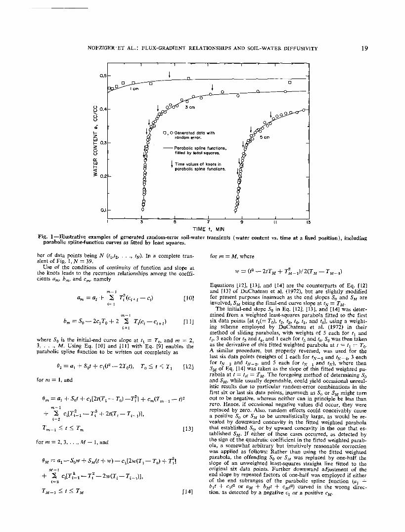
Several examples of random-error transients are illustrated inFig. 1. The solid-line curves through the data are an importantpart of the diffusivity analysis of the present paper, the furtherdevelopment and calculations of which we shall now consider indetail. It should be emphasized, however, that although theproblem of equations [5] to [8] is being used for purposes ofillustration and testing, this does not in any way limit the pres-ent diffusivity method to this particular type of boundary-valueproblem.

Fitting and Calculational Procedure

STEP 1: FITTING OF WATER-CONTENT TRANSIENTSFor wetting conditions, a water-content transient (Fig. 1) is

generally a sigmoidal curve, originating from a small or zeroslope (at 8a = 0.10 in the present case), being concave up-ward at the lower water contents, passing through an inflection,becoming concave downward at still higher water contents, andapproaching zero slope at large times (maximal water con-tents). To accommodate these various features, the parabolicspline function of DuChateau et al. (1972) was fitted by leastsquares to the numerical values of 0(0 at given x. A parabolicspline function consists of a sequence of different parabolasjoined together at special points called knots (Fig. 1). At eachknot both the function and its first derivative were made con-tinuous.

Letting m — 1, 2, . . ., M denote any given parabolic sub-range of which there are M altogether, the parabolic equationof the w'th subrange is written

. = a [9]

subject to

where 8m is the water content, and am, bm, and cm are the con-stant, linear, and quadratic coefficients, respectively, of the m'thparabolic subrange generally delimited at its left end by theknot coordinate t = Tm-\ and at its right end by the knot coor-dinate / = Tm. Altogether there are M — 1 knots, with t coor-dinates Tv T2, . . . , TM_! as arranged in increasing order. Whenm = 1 the / coordinate T0 of the left end of the first parabolicsubrange is not a knot, but is simply taken as the / coordinate fxof the first data point (smallest time value). Likewise, for thelast (m — M) parabolic subrange, TM is taken as the t coordi-nate tN of the last data point (largest time value), the total num-

NOFZIGER ET AL.: FLUX-GRADIENT RELATIONSHIPS AND SOIL-WATER DIFFUSIVITY 19

0.5

80.4

8

0.3

OOQ:UJ

0.2

O.I

D, O Generated data withrandom error.

Parabolic spline functionsfitted by least squares.

Time values of knots inparabolic spline functions

13TIME t, MIN

Fig- 1—Illustrative examples of generated random-error soil-water transients (water content vs. time at a fixed position), includingparabolic spline-function curves as fitted by least squares.

her of data points being N (/1,?2, • • •, tK). In a complete tran-sient of Fig. 1, N = 39.

Use of the conditions of continuity of function and slope atthe knots leads to the recursion relationships among the coeffi-cients am, bm, and cm, namely

[10]

for m = M, where

bm = S0- [11]t=l

where S0 is the initial-end curve slope at tv — 7"0, and m = 2,3, . . ., M. Using Eq. [10] and [11] with Eq. [9] enables theparabolic spline function to be written out completely as

6, = a,

for m — 1, and

m-1

i-2

Tm_1 < t < Tm

for m = 2, 3, . . ., M - 1, and

c,(fl - 2T0r), [12]

[13]

„ = <*! — 50wAf-l

i=2

) — c1[2w(T1 - ro) + T2]

[14]

Equations [12], [13], and [14] are the counterparts of Eq. [12]and [13] of DuChateau et al. (1972), but are slightly modifiedfor present purposes inasmuch as the end slopes S0 and SM areinvolved, SM being the final-end curve slope at tN = TM.

The initial-end slope S0 in Eq. [12], [13], and [14] was deter-mined from a weighted least-squares parabola fitted to the firstsix data points [at ?t(= T0), tz, ts, t±, ts, and te~], using a weight-ing scheme employed by DuChateau et al. (1972) in theirmethod of sliding parabolas, with weights of 5 each for tl andt2, 3 each for ?3 and t4, and 1 each for ts and re. S0 was then takenas the derivative of this fitted weighted parabola at / = t± = T0.A similar procedure, but properly reversed, was used for thelast six data points (weights of 1 each for %_5 and tN_4, 3 eachfor CN_3 and 'N_2, and 5 each for (N_1 and tN), where thenSM of Eq. [14] was taken as the slope of this fitted weighted pa-rabola at t = tN = TM. The foregoing method of determining S0and 5M, while usually dependable, could yield occasional unreal-istic results due to particular random-error combinations in thefirst six or last six data points, inasmuch as S0 or SM might turnout to be negative, whereas neither can in principle be less thanzero. Hence, if occasional negative values did occur, they werereplaced by zero. Also, random effects could conceivably causea positive S0 or SM to be unrealistically large, as would be re-vealed by downward concavity in the fitted weighted parabolathat established S0, or by upward concavity in the one that es-tablished SM. If either of these cases occurred, as detected bythe sign of the quadratic coefficient in the fitted weighted parab-ola, a somewhat arbitrary but intuitively reasonable correctionwas applied as follows: Rather than using the fitted weightedparabola, the offending ,S0 or SM was replaced by one-half theslope of an unweighted least-squares straight line fitted to theoriginal six data points. Further downward adjustment of theend slope by repeated factors of one-half was employed if eitherof the end subranges of the parabolic spline function (ax +M + ci'2 or am + bMt + cMtz) curved in the wrong direc-tion, as detected by a negative Cj or a positive CM.

20 SOIL SCI. SOC. AMER. PROC., VOL. 38, 1974

10-

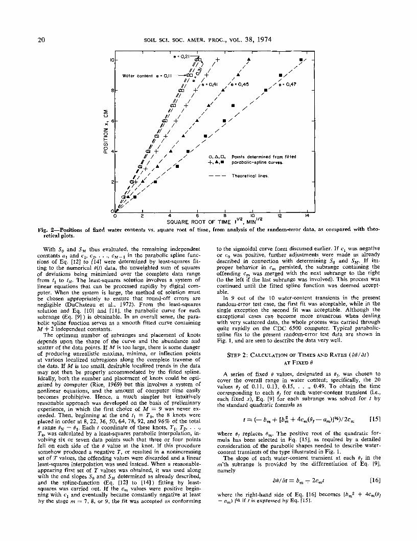
O, A, D, Points determined from fitted-f, A,B parabolic-spline curves.

14SQUARE ROOT OF TIME t , MIN

Fig. 2—Positions of fixed water contents vs. square root of time, from analysis of the random-error data, as compared with theo-retical plots.

With 50 and SM thus evaluated, the remaining independentconstants al and clt c2, . . ., CM_I in the parabolic spline func-tions of Eq. [12] to [14] were determined by least-squares fit-ting to the numerical 0(t) data, the unweighted sum of squaresof deviations being minimized over the complete data rangefrom ?j to /N. The least-squares solution involves a system oflinear equations that can be processed rapidly by digital com-puter. When the system is large, the method of solution mustbe chosen appropriately to ensure that round-off errors arenegligible (DuChateau et al., 1972). From the least-squaressolution and Eq. [10] and [11], the parabolic curve for eachsubrange (Eq. [9]) is obtainable. In an overall sense, the para-bolic spline function serves as a smooth fitted curve containingM + 2 independent constants.

The optimum number of subranges and placement of knotsdepends upon the shape of the curve and the abundance andscatter of the data points. If M is too large, there is some dangerof producing unrealistic maxima, minima, or inflection pointsat various localized subregions along the complete traverse ofthe data. If M is too small, desirable localized trends in the datamay not then be properly accommodated by the fitted spline.Ideally, both the number and placement of knots could be opti-mized by computer (Rice, 1969) but this involves a system ofnonlinear equations, and the amount of computer time easilybecomes prohibitive. Hence, a much simpler but intuitivelyreasonable approach was developed on the basis of preliminaryexperience, in which the first choice of M = 9 was never ex-ceeded. Then, beginning at the end tt = J0, the 8 knots wereplaced in order at 8, 22, 36, 50, 64, 78, 92, and 96% of the total9 range ON — 0j. Each t coordinate of these knots, Tj, T2> • • •>T8, was calculated by a least-squares parabolic interpolation, in-volving six or seven data points such that three or four pointsfell on each side of the 0 value at the knot. If this proceduresomehow produced a negative T, or resulted in a nonincreasingset of T values, the offending values were discarded and a linearleast-squares interpolation was used instead. When a reasonable-appearing first set of T values was obtained, it was used alongwith the end slopes S0 and Su determined as already described,and the spline-function (Eq. [12] to [14]) fitting by least-squares was carried out. If the cm values were positive begin-ning with Cj and eventually became constantly negative at leastby the stage m = 7, 8, or 9, the fit was accepted as conforming

to the sigmoidal curve form discussed earlier. If Cj was negativeor c9 was positive, further adjustments were made as alreadydescribed in connection with determining S0 and $M. If im-proper behavior in cm persisted, the subrange containing theoffending cm was merged with the next subrange to the right(to the left if the last subrange was involved). This process wascontinued until the fitted spline function was deemed accept-able.

In 9 out of the 10 water-content transients in the presentrandom-error test case, the first fit was acceptable, while in thesingle exception the second fit was acceptable. Although theexceptional cases can become more numerous when dealingwith very scattered data, the whole process was carried throughquite rapidly on the CDC 6500 computer. Typical parabolic-spline fits to the present random-error test data are shown inFig. 1, and are seen to describe the data very well.

STEP 2: CALCULATION OF TIMES AND RATES ( 8 9 / d t )AT FIXED 6

A series of fixed 8 values, designated as fy, was chosen tocover the overall range in water content; specifically, the 20values Bf of 0.11, 0.13, 0.15, . . ., 0.49. To obtain the timecorresponding to each 0f for each water-content transient (i.e.,each fixed x), Eq. [9] for each subrange was solved for t bythe standard quadratic formula as

[15]

where 8f replaces 8m. The positive root of the quadratic for-mula has been selected in Eq. [15], as required by a detailedconsideration of the parabolic shapes needed to describe water-content transients of the type illustrated in Fig. 1.

The slope of each water-content transient at each 8S in them'th subrange is provided by the differentiation of Eq. [9],namely

: bm + 2cmt [16]

where the right-hand side of Eq. [16] becomes [6m2 + 4cm(fff

- om) ]% if t is expressed by Eq. [15].

NOFZIGER ET AL.: FLUX-GRADIENT RELATIONSHIPS AND SOIL-WATER DIFFUSIVITY 21

^

1.5

VJ^"zs2<-> I.O

roXroLUQ.0

^0.5

0.0

^Extrapolated points for first~ three data sets (O, D and +).

O Data for t = 8.69 min (time at whichat x = 5.0 cm, and t"2 = 2.95

D Data for t = 9.47 min (time at which1/2at x « 5.0 cm, and t • 3.O8

1 ' 1

^\

e • 0.11 ~*"\min"2). \,

e = 0.31 a.min"2). \ A

* _*_+ Data for t = 24.67 min (time at which e = O.45 \

at x = 5.O cm, and t"2 = 4.97 min"2). °

A Data for t • 43.40 min (time at which e = 0.47 \at x • 5.O cm, and t"2 = 6.59 min"2), but not 'used to determine flux or an extrapolated point.

— — — Theoretical curve.

. 1 , 1

\Q -

\\

O.I O.2 0.3WATER CONTENT e, CC/CC

O.4 0.5

Fig. 3—Slope dx/du vs. water content for several fixed times, from analysis of the random-error data, as compared with the theo-retical curve.

STEP 3: POSITION TRANSIENTS AND CALCULATION OFWATER-CONTENT GRADIENTS

In conjunction with the x positions known for the water-content transients, the t values calculated from Eq. [15] pro-vided numerical values of the position transients x(t) at 6S. Inusing these data to determine dx/dt, preliminary experience in-dicated the desirability of considering A: as a function of thevariable u = fi, where 0 < 7 < 1, since a well-chosen value of7 produces a marked reduction in the considerable curvaturenormally exhibited by x(t). For the data of the present testcases as generated from Eq. [5] to [8], it is known that x vs.;i/2 wju be proportional; hence, 7 was taken as Vz. Even forproblems in which 7 — Vi does not produce perfect linearity,it nevertheless provides a plot of much less curvilinearity thandoes x vs. t, and thus constitutes a good starting point even iffurther refinement is to be desired and undertaken. Typicaldata of x vs. u (= f1/2) are shown in Fig. 2 for the random-error test case. Not only do the points exhibit generally goodlinearity, but they also conform very well to their respectivetheoretical lines, thus providing excellent validation of the vari-ous calculations carried out thus far.

With x(t) transformed to x(u), differentiation yields

With dx/du thus evaluated at each Sf and at each t calcu-lated from Eq. [15], each dx/dt at these same B, and t wasthen calculated from Eq. [17] (with 7 = Vi). Correspondingwater-content gradients —de/dx were then calculated from Eq.[3], where the 86/dt were those determined in Step 2 fromEq. [16].

STEP 4: DETERMINATION OF THE FLUX

At each fixed / calculated by Eq. [16], the dx/du evaluatedin Step 3 were treated as a function of 6, with typical plots asshown in Fig. 3 for the random-error test case. Once again, thedata points conformed very well to the theoretical curve knownfrom the solution generated from Eq. [5] to [8]. To these curvesof dx/du vs. 6, Eq. [4] was applied in conjunction with Eq. [17],the flux at fy and fixed t thus becoming

refM (dx/du)d9. [18]

dx/dt = yf-1 (dx/du). [17]

The derivative dx/du was then computed from the X-VS-H databy the method of sliding parabolas (DuChateau et al., 1972).Briefly, a parabola was fitted by weighted least squares to agroup of six consecutive data points, the six-point group beingmoved and refitted successively throughout the complete rangeof the data. Normally, only the center interval of the five-interval (six-point) fitting group was the region considered tobe described by a given parabolic fit, and the slope anywherewithin this center interval was taken as the derivative of thefitted parabola in the same way as Eq. [16] was used for theparabolic spline. Right at a data point, which is the junction be-tween two intervals, the slope was taken as the arithmetic meanof the two fitted sliding-parabolic slopes obtained by approach-ing the data point from both left and right. Complete details ofthe least-squares weighting scheme used in the sliding-parabolamethods are given by DuChateau et al. (1972).

To carry out the integration in Eq. [18], a value of dx/dumust somehow be supplied at 00(=0.10), since 0.11 is thesmallest e at which dx/du is provided as a matter of course.For each curve of dx/du vs. e, the needed additional point wasgenerated by fitting an unweighted least-squares straight line tothe six points nearest to Ba (» of 0.11, 0.13, 0.15, 0.17, 0.19,0.21 in Fig. 3), taking the intersection of this line with e = 0aas the extrapolated value of dx/du at 6a. Integration from Bato Of (Eq. [18]) was performed by six-point sliding parabolas(DuChateau et al., 1972) fitted between each two data points,integrating between each two data points by means of this fittedparabola, and then summing these piecewise integrations from6a onward until the desired 0f was reached. This sum was thenmultiplied by 7^-1 — l/(2/V4), to obtain the flux of eq. [18].

Since the sliding-parabola integrations here described did re-quire a minimum of six data points, the flux was not calculatedat times for which there were fewer than six points. This oc-curred primarily at high water contents for the last one or twowater-content transients. Also, for very large times and low wa-ter contents there may be too few data points for x vs. u as well

22 SOIL SCI. SOC. AMER. PROC., VOL. 38, 1974

0.3

CCQJ

0.0

lO rt^- /V r\ j>

o ls~ ~ '

• 'i / /i1 1 ' '-O/ ' /if / / /1 ' • / /•[i /' / /jf/ / / /

*a • ' /

§§/{** °'°' ^

to^^-^^^ — —

,, •

7 % \ 9

y°' ^..035^ ^^33

/ / /f /

// / X// xX

V7 OX""

XX ''^ J3x -^ x*^x ^^ ^e-0.27-^.^-

x-^A n ^5--" _

-̂'lv_::: ::::---"

1 i

= water content

• •031

•re = 0.29 -/ x-'

\"^^

Theoretical lines.

r:0.25-̂ ? -

pe = O.23 —— -7i. ——— ——*

r-e « O.I9— i

0.5 1.0 1.5 2.0WATER-CONTENT GRADIENT -9e/ax, CM

Fig. 4 — Water flux vs. water-content gradient at different fixed water contents, from analysis of the random-error data, as comparedwith theoretical plots.

as for Sx/du vs. 6. In such cases, fluxes were not calculatedbecause of the extrapolation error involved in generating thepoint for dx/du at ea.

STEP 5: DETERMINATION OF SOIL-WATER DIFFUSIVITY

Steps 3 and 4 provided the data to enable flux v to be plottedagainst gradient —dff/dx at various fixed 9, the number of flux-gradient pairs being less than or equal to the number of water-content transients. Typical plots of such data for the random-error test case are shown in Fig. 4. The data points conformvery satisfactorily to their corresponding theoretical lines thatare known from the solution of Eq. [5] to [8]. A calculation ofthe Buckingham-Darcy soil-water diffusivity was thus justifia-ble, and was made as D = v/(—de/dx) for each flux-gradientpair of a given fy, the arithmetic mean of all these individualdiffusivities then being taken as D(ef). Repeating the processfor each 6f then enabled D to be plotted against fy, as an ex-pression of the diffusivity function D(0).

RESULTS AND DISCUSSION

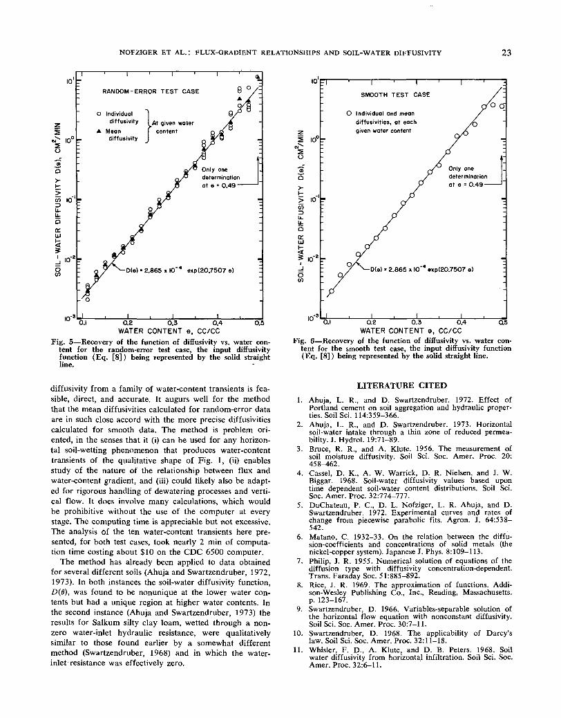
Diffusivities versus water contents for the random-errortest case are shown in Fig. 5. The open circles representindividual calculations of diffusivity, while the solid trian-gles are the arithmetic means of the individual values at thegiven water contents. The number of points in each meanis ten for 6 of 0.11 to 0.17, nine for e of 0.19 to 0.37, eightfor 9 of 0.39 to 0.41^ seven for 6 = 0.43, five for 6 =0.45, four for 6 = 0.47, and one for 6 = 0.49. At eachwater content, both the largest and smallest diffusivities arealways plotted along with the mean, with as many other in-dividual values being included as can be done without un-due crowding. The straight line is the graph of Eq. [8], theknown diffusivity function used to generate the water-con-tent transients for both the random-error and smooth testcases. It is clear that the diffusivities calculated by the pres-ent method fall upon the straight line in highly acceptable

fashion. The individual diffusivities are within ±50% ofthe known diffusivity function, with the exception of onlythree values (at 6 of 0.45 and 0.47) of which the most dis-crepant is +127% in error. The mean diffusivities arewithin ±25% of the known diffusivity function, with thetwo exceptions (at 9 of 0.45 and 0.49) being +54% inerror.

Diffusivity results for the smooth test case are shown inFig. 6, with the number of determinations at each watercontent being the same as in Fig. 5. The individual diffu-sivities at a given water content agreed with each otherwithin the accuracy of plotting. Thus, each circular symbolalso represents the mean diffusivity at that water content.These values are within ±25% of the known diffusivityfunction (Eq. [8]) expressed by the straight line, with theexception of the value at the highest water content (8 =0.49) where the error is —53%. It thus appears that themean diffusivities in Fig. 5 are behaving almost identicallyto the data points in Fig. 6, as regards their proximity toand maximum departure from the known diffusivity func-tion. The absence of random errors in the generated dataseems primarily to produce (Fig. 6) an improved precision(lack of scatter) in the calculated diffusivity at a givenwater content, but these calculated values (equivalent tomeans) are still distributed with a small degree of errorabout the known (true) diffusivity function. Whether thelast two points in Fig. 6 represent a real trend of slight cal-culational depression of diffusivity cannot be ascertained atpresent, apart from further computations performed moreintensively in that water-content region.

From the various results here obtained, not only in thefinal sense of Figs. 5 and 6 but also on the basis of Figs.1 to 4 as validating the various intermediate stages of analy-sis, it is concluded that the present method of determining

NOFZIGER ET AL.: FLUX-GRADIENT RELATIONSHIPS AND SOIL-WATER DIFFUSIVITY 23

IO'T

z5^- ioc

o

sQ

55 10"'u-u.ocrLUi', I0"2

8

10"

RANDOM-ERROR TEST CASE

O Individualdiffusivity

A Meandiffusivity

Dte) = 2.865 x 10"* exp(2O.7507 e)

- O

O.I

lO'FT

O.50.2 0.3 0.4WATER CONTENT e, CC/CC

Fig. 5—Recovery of the function of diffusivity vs. water con-tent for the random-error test case, the input diffusivityfunction (Eq. [8]) being represented by the solid straightline.

I 10'

o

-£Q

> »•'COo

Qo:UJ

i.o-<o<r>

10

^ I ' ISMOOTH TEST CASE

O Individual and meandiffusivities, at eachgiven water content

O O

D(e) = 2.865 x IO"* exp(20.7507 e)

>-3 _L0.1 Q50.2 0.3 0.4

WATER CONTENT e, CC/CCFig. 6—Recovery of the function of diffusivity vs. water con-

tent for the smooth test case, the input diffusivity function(Eq. [8]) being represented by the solid straight line.

diffusivity from a family of water-content transients is fea-sible, direct, and accurate. It augurs well for the methodthat the mean diffusivities calculated for random-error dataare in such close accord with the more precise diffusivitiescalculated for smooth data. The method is problem ori-ented, in the senses that it (i) can be used for any horizon-tal soil-wetting phenomenon that produces water-contenttransients of the qualitative shape of Fig. 1, (ii) enablesstudy of the nature of the relationship between flux andwater-content gradient, and (iii) could likely also be adapt-ed for rigorous handling of dewatering processes and verti-cal flow. It does involve many calculations, which wouldbe prohibitive without the use of the computer at everystage. The computing time is appreciable but not excessive.The analysis of the ten water-content transients here pre-sented, for both test cases, took nearly 2 min of computa-tion time costing about $10 on the CDC 6500 computer.

The method has already been applied to data obtainedfor several different soils (Ahuja and Swartzendruber, 1972,1973). In both instances the soil-water diffusivity function,D(6), was found to be nonunique at the lower water con-tents but had a unique region at higher water contents. Inthe second instance (Ahuja and Swartzendruber, 1973) theresults for Salkum silty clay loam, wetted through a non-zero water-inlet hydraulic resistance, were qualitativelysimilar to those found earlier by a somewhat differentmethod (Swartzendruber, 1968) and in which the water-inlet resistance was effectively zero.