FLUORESCENCE BASED OPTICAL SENSOR FOR PROTEIN DETECTION

by

Kailiang Sun

Rakesh Kapoor, CHAIR Christopher M Lawson

Upender Manne

A THESIS

Submitted to the graduate faculty of The University of Alabama at Birmingham,

in partial fulfillment of the requirements for the degree of Master of Science

BIRMINGHAM, ALABAMA

2008

FLUORESCENCE BASED OPTICAL SENSOR FOR PROTEIN DETECTION

Kailiang Sun

DEPARTMENT OF PHYSICS

ABSTRACT

This work mainly involves detection of protein by fluorescence based optical

sensors. One is the profile design of optical fiber serving as a type of biosensors, the

other is the study of an improved fluorescence polarization immunoassay (FPI) method

using antibody coated magnetic nanoparticles.

A theoretical model using ray tracing method is developed to design the probe. The

model could explain the observed fact that the maximum signal for a given realistic

tapered length is at a probe radius smaller than that expected from V-number matching

condition. It is shown that to obtain maximum fluorescence signal a realistic optimum

taper length needs to be chosen. We found that, in air environment, this requirement is

easy to achieve than that in aqueous condition. These facts were confirmed

experimentally.

A novel idea is proposed with regard to FPI, that to introduce antibody coated

magnetic nanoparticles into this immunoassay can greatly enhance the detecting range of

biomolecules with various molecular weights. Detailed scheme is described in this work

including related optical setup construction method, suitable dye and magnetic

nanoparticle selection, magnetic field construction strategy, method of data processing,

ii

etc. Experimental setup was built up and preliminary experiments have been carried on

towards the development of this method. A homogeneous immunoassay was performed,

and enhanced fluorescence anisotropy was observed with increasing amount of

antibodies, which validated the usability of the optical setup. The developed FPI method

using magnetic nanoparticles can be used for sensitive protein detection in future.

iii

ACKNOWLEDGMENTS

I would like to thank Dr. Rakesh Kapoor, my advisor, for his guidance and instructions over my

graduate study. Without him, none of my research would have been possible. I would like to thank

Drs. Christopher Lawson and Upender Manne for being my graduate study committee members. I

would like to thank Drs. Renato Camata and Joseph Harrison, as well as Drs. R. Kapoor and C.

Lawson who have delivered advanced physics courses to me. And I would like to thank Chun-wei

Wang, my colleague and friend, for helping me in doing experiments. Also I would like to thank all

the other professors, staff, and graduate students who have given me generous help in conducting my

research. Finally, I would like to thank Dr. Vohra, Dr. Shealy and our department for providing the

financial support for me to perform research.

iii

TABLE OF CONTENTS

ABSTRACT..................................................................................................................................... ii ACKNOWLEDGMENTS............................................................................................................... iii LIST OF TABLES........................................................................................................................... vi LIST OF FIGURES........................................................................................................................ vii CHAPTER 1 .....................................................................................................................................1 INTRODUCTION.............................................................................................................................1

Thesis Outline ...........................................................................................................................4 REFERENCES..................................................................................................................................5 CHAPTER 2 .....................................................................................................................................7 OPTIMUM PROBE DESIGN FOR MAXIMUM FLUORESCENCE SIGNAL FROM AN EVANESCENT WAVE FIBER OPTIC BIOSENSOR .....................................................................7

Introduction ...............................................................................................................................7 Theory .......................................................................................................................................9

Ray Trajectory in a Tapered Fiber ...................................................................................12 Characteristics of Evanescent Wave................................................................................14

Absorption of Evanescent Power. ...........................................................................15 Fluorescence Signal from Combination Fiber.................................................................16

Evanescent Absorption. ...........................................................................................16 Fluorescence Coupling Back Efficiency..................................................................19

Experiments.............................................................................................................................20 Probe Preparation ............................................................................................................20 Experimental Setup .........................................................................................................21 Results and Discussion....................................................................................................22

Conclusions .............................................................................................................................25 REFERENCES................................................................................................................................27 CHAPTER 3 ...................................................................................................................................29 INTRODUCTION...........................................................................................................................29

Backgorund of Magnetic Nanoparticles Usage.......................................................................29 Fluorescence Polarization Theory ...........................................................................................31 Some Explanations of Anisotropy Theory ..............................................................................35

Calculation of Rotational Correlation Time of Proteins..................................................35

Why Is the Total Intensity Equal to 2I I⊥+ ? ................................................................37

CHAPTER 4 ...................................................................................................................................38 NOVEL IDEA INTRODUCED TO FPI .........................................................................................38 CHAPTER 5 ...................................................................................................................................41

iv

KNOWLEDGE OF MAGNETISM FOR DETERMING SUITABLE NANOPARTICLES TO BE USED ..............................................................................................................................................41

Definitions and Units ..............................................................................................................41 Classes of Magnetic Materials ................................................................................................42

Diamagnetism .................................................................................................................43 Paramagnetism ................................................................................................................43 Ferromagnetism...............................................................................................................44 Ferrimagnetism................................................................................................................45 Antiferromagnetism ........................................................................................................45 Superparamagnetism. ......................................................................................................46

What Kind of Magnetic Particles Are Suitable for This Purpose? ..........................................48 Possibility to Extract the Signal ..............................................................................................51 Commercial Sources of Dye and Magnetic Nanoparticles......................................................51

CHAPTER 6 ...................................................................................................................................53 EXPERIMENTAL PART ................................................................................................................53

Magnetic Field Construction Strategy.....................................................................................53 DC Magnetic Field Construction and Calibration...................................................................58 Optical Setup...........................................................................................................................59

Glan-Thompson Polarizer ...............................................................................................60 Glan-Taylor Polarizer ......................................................................................................62

CHAPTER 7 ...................................................................................................................................64 FA Meaurement and Data Processing .............................................................................................64 CHAPTER 8 ...................................................................................................................................68 RESULTS AND DISCUSSIONS....................................................................................................68

Determine the G Factor ...................................................................................................68 Validation of the FA Measurement System .....................................................................68

CHAPTER 9 ...................................................................................................................................71 CONCLUSIONS AND FUTURE WORK......................................................................................71 REFERENCES................................................................................................................................72

v

LIST OF TABLES

Tables Pages Table 5-1 Magnetic units.........................................................................................................42 Table 5-2 Differences between paramagnetism and ferromagnetism......................................45 Table 6-1 Magnetic field versus current..................................................................................59 Table 7-1 Comparison on sensitivity of two spectrometers to polarized light ........................65 Table 8-1 Measurements for determining G factor..................................................................68 Table 8-2 Calculated FA data of immunoassay for rabbit-anti-goat IgG.................................69

vi

LIST OF FIGURES

Figures Pages

Figure 2.1. Combination tapered fiber.......................................................................................9 Figure 2.2. Equivalent geometrical path of optical ray in a linear tapered part of combination

fiber probe. ......................................................................................................................11 Figure 2.3. Optimum probe radius and taper length in terms of taper angle. ..........................15 Figure 2.4. A photograph of a typical combination fiber. ....................................................21 Figure 2.5 Experimental setup. LD- Laser Diode, CL- Collimation Lens, BF- Band-pass Filter,

ND- Neutral Density filter, LF -Long-pass Filter and SF- Short-pass Filter...................24 Figure 2.6. Variation of fluorescence signal with probe radius. A comparison of simulation and

experimental result. .........................................................................................................24 Figure 3.1. Intuitive illustration of a Fluorescence polarization immunoassay. f is the rotation

correlation time. ..............................................................................................................31 Figure 3.2. Molecular-weight-dependent anisotropy for a protein-bound luminophore with

luminescence lifetimes of 5, 50, 1000, and 3000 ns........................................................36 Figure 3.3. Polarization of Fluorescence.................................................................................37 Figure 3.4. Dipole radiation pattern ........................................................................................38 Figure 5.1. Brownian relaxation time versus MNP diameter. T=300 K. .................................49 Figure 5.2. Relaxation times of Brownian and Neel relaxation versus MNP core diameter. K=20

kJ/m3 and T=300 K were assumed. .................................................................................49 Figure 6.1. Magnetic field calculation of a segment of straight wire carrying current. ..........54 Figure 6.2. Cartesian coordinate system for the rectangular helmholtz coils..........................55 Figure 6.3. Magnetic field contour of the designed helmholtz coils. ......................................56 Figure 6. 0.4. Mounting spools onto testing cube (not to scale)............................................57 Figure 6.5. Coil spools design scheme. ...................................................................................58 Figure 6.6. Experimental setup of Fluorescence Polarization. ................................................60 Figure 6.7. Glan Thomson Polarizer........................................................................................61 Figure 6.8. A Glan-Taylor prism .............................................................................................62 Figure 8.1. Steady-state fluorescence anisotropy of Alexa Fluor 430 labeled rabbit-anti-goat IgG

at various concentrations of goat-anti-rabbit IgG measured at 20 .............................70 C

vii

CHAPTER 1

INTRODUCTION

As for the detection of bio-molecules such as proteins, the traditional methods are

radioimmunoassay (Wide 1966), Enzyme-Linked ImmunoSorbent Assay (ELISA)

(Engvall 1971) and western blot (Burnette 1981). However researchers wish to develop

new approaches to enhance the detection capability, or enable researchers to study the

characteristics of biomaterials of interest. The developments of fluorescence materials

that have sound photophysical properties provide convenience to the study of biological

principles using optical devices. Some research work has been conducted on the

fluorescence based immunoanalytical systems (Marquette, 2006). The emphases of this

thesis will be focused on the further development of fluorescence based fiber optical

sensing (Wolfbeis 2006, Campbell 2006, Ko 2006) and fluorescence polarization

immunoassay (FPI) (Shim 2004, Tsuruoka, 1991).

In recent years fiber-optic biosensors attract considerable research effort because of

their potential sensitivity, detection speed and adaptability to a wide variety of assay

conditions. In a fiber optic sensor, a fiber probe acts as a transduction element. It can

generate absorption, fluorescence or scattering signal that proportions to analyte. There

are various kinds of fiber optic sensors (Ahmad 2005, Anderson 1994, Golden 1994), one

1

of the most sensitive fiber-optic biosensor is based on excitation and detection of

fluorescence using evanescent wave associated with the propagating modes in an optical

fiber. Lots of work has been done with the aim of enhancing the acquisition efficiency of

fluorescence signal (Kapoor 2004, Prasad 2003)

The design of fiber probe is a crucial factor for enhancing the signal-to-noise ratio in

a fiber-optic sensor. The most popular fiber probes currently under study are long tapered

probe (Anderson 1994, Geng 2004) and fiber with a thin waist as the probe part (Guo

2003, Villatoro 2004). The first kind of probe shape can be easily achieved by molding

with polystyrene material, and the second combination shape is usually made by torching

and stretching glass fibers. By comparative study of the signal acquisition from straight

fiber and tapered optical fibers theoretically, we have shown that combination tapered

fiber, which has a shape of combination of tapered part and straight part, have the highest

sensitivity than fibers with other kinds of shape. In this thesis, we propose a combination

probe shape using glass fiber. This will have the advantage that it will have very low

noise signal which is typically generated by carbon constituent in plastic fiber. With the

help of acid etching method, very long probe part can be obtained which is relatively

difficult to be achieved by torching and stretching method. Although this kind of probe

shape has already been studied in some theoretical work (Nath 1998), a more detailed

mathematical model is needed which describes the relationship between fluorescence

intensity and parameters like probe radius and refractive index of the environment. Some

studies show that the taper angle of the taper part will affect the factors like transmission

2

and penetration depth, and finally the fluorescence intensity obtained (Guo 2003, Angela

2006). However, a thorough study of the effect of the taper part on the collected

fluorescence is still lacking. A criterion needs to be established for the optimum

parameters of the taper zone for optimum signal generation and collection.

Another promising area is fluorescence polarization immunoassay which is

presently in widespread commercial use in several instruments and still has a vast area to

be explored (Shim 2004, Tsuruoka 1991, Li 2007). Briefly, the fluorescence polarization

of a labeled macromolecule depends on the fluorescence lifetime and the rotational

correlation time. For the use in analytical biochemistry, the antigen-antibody interactions

and hormone-receptor interactions will change the rotational correlation time of the

labeled molecules, the change of polarization anisotropy ensuing (Dandliker 1973). This

method has an essential limitation that when it comes to the detection of large weight

molecules, the anisotropy changes little which limits the dynamic range of the FPI

method. Some studies make use of luminescent complex which has advanced

characteristics like long lifetimes, high quantum yields and high emission polarization

etc. to reduce the limitation of FPI (Guo 1998). Another approach which is proposed in

this thesis could be to increase the weight of unlabeled molecules by attaching

nanoparticle. Due to the high weight of nanoparticle used, a great dragging effect will

happen to the targeted protein after immunoreaction. This will result in a change in

fluorescence polarization. Based on this, an ensuing idea is proposed which in principle

can further enhance the capacity of this method, that is to use antibody coated magnetic

3

particles in the FPI, so that a switching magnetic field can be applied to modulate the FP

change.

Thesis Outline

This thesis is organized in the following way: It contains two parts-Part I including

Chapter 2 will describe the design aspect of an optical fiber sensor, which is reprinted

from published paper1 and reprint permission has been granted by the publisher.

Part II including the following chapters will mainly focused on the development of

FPI method using antibody coated magnetic nanoparticles.

1 Kailiang Sun and Rakesh Kapoor, “Optimum taper length for maximum fluorescence signal from an evanescent wave fiber optic biosensor.” Optical Fibers and Sensors for Medical Diagnostics and Treatment Applications VIII, 68520U, SPIE Proceedings Volume 6852, (2008).

4

REFERENCES

Ahmad, M. and L.L. Hench, “ Effect of taper geometries and launch angle on evanescent wave penetration depth in optical fibers.” Biosensors and Bioelectronics 20 (7):1312-1319, 2005.

Anderson, G. P. , J. P. Golden, et al. (1994). “An evavescent wave biosensor. I. Fluorescent signal acquisition from step –etched fiber optic probes.” Biomedical Engineering, IEEE Transactions on 41(6): 578-584

Angela Leunga, K.R., P. Mohana Shankarb and Raj Mutharasan, “Effects of geometry on transmission and sensing potentiall of tapered fiber sensors,” Biosensors and Bioelectronics 21 (12):2202-2209, 2006.

Burnette, W. Neal, “Western blotting': electrophoretic transfer of proteins from sodium dodecyl sulfate — polyacrylamide gels to unmodified nitrocellulose and radiographic detection with antibody and radioiodinated protein A,” Anal Biochem 112 (2): 195-203, 1981.

Campbell, D.W., C. Muller, et al. , “Development of a fiber optic enzymatic biosensor for 1, 2-dichloroethane”, Biotechnology Letters 28 (12):883-887, 2006.

Dandliker, W. B.; Kelly, R. J.; Dandliker, J.; Farquhar, J.; Levin, J. Immunochemistry 1973, 10, 219-227.

Engvall E, Perlman P, “Enzyme-linked immunosorbent assay (ELISA). Quantitative assay of immunoglobulin G”. Immunochemistry 8 (9): 871-4, 1971.

Geng, T., Mark T. Morgan, and Arun K. Bhunia, “Detection of Low Levels of Listeria monocytogenes Cells by Using a Fiber-Optic Immunosensor.” Applied and Environmental Microbiology 70 (10):6138-6146, 2004.

Golden,J.P., Anderson,G.P.,Rabbany,S.Y.,Ligler,F.S., “An Evanescent Wave Biosensor-Part II: Fluorescent Signal Acquisition from Tapered Fiber Optic Probes,” IEEE Transactions on Biomedical Engineering. 41.6. June 1994

Guo, S.P. and S. Albin, “ Transmission property and evanescent wave absorption of cladded multimode fiber tapers.” Optics Express 11 (3):215-223, 2003.

Guo, X.Q., F. N. Castellano, et al., “Use of a Long-Lifetime Re(I) Complex in Fluorescence

5

Polarization Immunoassays of High-Molecular-Weight Analytes”, Anal. Chem. 70:632-637, 1998

Kapoor,R., Kaur N., Nishanth, E.T., Halvorsen,S.W., Bergey,E.J., Prasad,P.N., “Detection of trophic factor activated signaling molecules in cells by a compact fiber-optic sensor,” Biosensors and Bioelectronics 20, 345-349, 2004.

Ko, S.H. and S.A. Grant, “A novel FRET-based optical fiber biosensor for rapid detection of Salmonella typhimurium,” Biosensors & Bioelectronics 21 (7):1283-1290, 2006.

Li, W., “Probing rotation dynamics of biomolecules using polarization based fluorescence microscopy. Microscopy Research and Technique,” 70: 390-395, 2007.

Marquette, C.A. and L. J. Blum, “State of the art and recent advances in immunoanalytical systems,” Biosensors & Bioelectronics 21 (8):1424-1433, 2006.

Nath,N.,Anand,S., “Evanescent wave fiber optiic fluorosensor:effect of tapering configuration on the signal acquisition,” Opt. Eng. 37 (1)220-228, January1998

Prasad,P.N., Introduction to Biophotonics. Wiley, New York, pp.327-334, 2003.

Shim, W.-B., A.Y.Kolosova, et al., “Fluorescence polarization immunoassay based on a monoclonal antibody for the detection of ochratoxin A,” International Journal of Food Science and Technology. 39: 829-837, 2004.

Tsuruoka, M., E. Tamiya, et al. “Fluorescence polarization immunoassay employing immobilized antibody,” Biosensors and Bioelectronics 6 (6): 501-505, 1991.

Villatoro, J.D. Monzon-hernandex, etal, “In-line optical fiber sensors based on cladded multimode tapered fibers.” Applied Optics 43 (32): 5933-5938, 2004.

Wide L, Porath J. , “Radioimmunoassay of proteins with the use of Sephadex-coupled antibodies,” Biochem Biophys Acta 30:257-260, 1966.

6

CHAPTER 2

OPTIMUM PROBE DESIGN FOR MAXIMUM FLUORESCENCE SIGNAL FROM AN EVANESCENT WAVE FIBER OPTIC BIOSENSOR

Introduction

In recent years fiber-optic biosensors attracted considerable research effort (Love

1992, Axelrod 2001, Willer 2002, Amad 2005) because of their potential sensitivity,

detection speed and adaptability to a wide variety of assay conditions. Their use as a

probe or as a sensing element is increasing in clinical, pharmaceutical, industrial and

military applications. Other main points in favor of the use of optical fibers in biosensors

are excellent light delivery, long interaction length, low cost and ability not only to excite

the target molecules but also to capture the emitted light from the targets. In a fiber optic

sensor, a fiber probe acts as a transduction element. It can generate absorption,

fluorescence or scattering signal that is proportional to the analyte concentration. There

are various kinds of fiber optic sensors (Golden 1994, Kapoor 2004), one of the

potentially sensitive fiber-optic biosensor is based on generation of fluorescence signal

using evanescent waves associated with the propagating modes in an optical fiber. There

are two main difficulties faced in fiber-based evanescent wave biosensors. Firstly, in

comparison to distal end biosensors, only a small amount of power is available in the

7

evanescent wave sensors for generating a fluorescence signal (Snyder 1983). Secondly, in

signal acquisition, there is only a low coupling efficiency of the fluorescence signal back

to the fiber itself (Thompson 1995). Thus, there is a critical need for optimum design and

fabrication of the fiber-based optical sensor leading to high excitations and a high level of

fluorescence signal acquisition at the output end of the fiber.

In a fiber probe to generate an evanescent wave excited signal from the probe

sensing region, cladding needs to be removed from the core along the distal end of a

step-index optical fiber. An analyte recognition element needs to be immobilized on the

decladded core region (Golden 1994). The decladding of core in the probe region leads to

inefficient coupling back of fluorescence due to a mismatch between the V-number of

probe and the cladded fiber part. It had been shown (Golden 1994) experimentally that

Probes created with reduced sensing region radius exhibit improved response as reduced

probe radius leads to reduction of V-number mismatch. It is further shown that tapering

the radius of probe region can further improve the response. The most popular fiber

probes currently under use are tapered fiber probes (Anderson 1994, Geng 2004).

Detailed theoretical studies based on ray-tracing method have shown that the tapered

optical fibers have higher sensitivity compared to straight fibers (Nath 1998) Theoretical

work has also shown that among the tapered fibers, combination tapered fibers have

higher sensitivity than continuous tapered fibers (Nath 1998). A combination tapered

fiber has a shape of combination of tapered part and a straight part (Figure 2.1).

8

In this paper we are reporting the design conditions for an optimum fiber probe. A

mathematical model based on ray tracing method is developed. The mathematical model

is used to find variation of the total signal intensity with probe parameters, such as probe

radius, taper length and refractive index of the environment. These theoretical results are

compared with the experimental results obtained from in house fabricated combination

taper fiber probes.

Figure 2.1. Combination tapered fiber. It has a linear tapered fiber sandwiched between a straight uncladded smaller diameter fiber (probe portion) and a cladded larger diameter fiber.

Theory

If we ignore the non-meridional rays, we can use a two-dimensional ray tracing

model to simplify the problem. In an evanescent wave fiber optic based sensor, the

evanescent wave generated on the fiber core is accessed by removing the cladding from a

section of the fiber. Specific fluorphore labeled analytes are immobilized on the exposed

9

fiber core. These analytes are monitored by detecting the coupled back fluorescent signal.

The eventual fluorescent signal is the product of two processes. First is the excitation of

fluorescence through the evanescent wave component of all the propagating rays inside

the fiber. Second is the fraction of total emitted fluorescence coupling back into the

detection end.

Removal of cladding, however, results in critical angle mismatch between the clad

portion and the sensing portion of the fiber. Critical angle becomes larger for the cladded

region than that of the sensing region, where an aqueous medium or air replaces the

cladding. Critical angle cα is defined in terms of the core refractive index and

cladding refractive index as

con

cln

1 cl

co

sincnn

α − ⎛ ⎞= ⎜

⎝ ⎠⎟ (1)

On the basis of geometric optics we can make an argument that out of all the

fluorescence rays generated on the probe surface only those can get coupled back into the

fiber, which make an angle α with the normal to the interface such that 2 / 2cα α π≤ ≤ ,

where 2cα is the critical angle in the uncladded probe part. When the fluorescence rays

reach back in the cladded fiber zone, only rays satisfying the condition / 2cα α π≤ ≤

can enter that zone and rest will be lost. Refractive index of cladding in the probe zone is

taken as the refractive index of the aqueous solution or air. Since , therefore aqn aq cln n<

2c cα α> , where cα is the critical angle in cladded zone. Now out of all the coupled

back fluorescence rays in the probe zone, the rays making angle in the range

10

2c cα α α≤ ≤ will be lost after reaching the cladded fiber zone. This observation

indicates that the fluorescence coupling back efficiency can be improved if some how the

y angle ra α can be continuously increased as the ray propagate from the probe portion

of fiber to the cladded or detection portion of fiber.

Another important factor responsible for generation of fluorescence signal in a fiber

probe is the number of reflections (total internal) an excitation ray makes in the probe

portion. Each such reflection generates evanescent field on the probe surface. Since

signal is always proportional to the total strength of evanescent field per unit area,

therefore larger the number of these reflections in probe zone better it is. If a ray makes

an angle θ with the fiber axis, the number of reflections per unit length f , in a straight

fiber with radius can be given as: r

1cot

fr θ

= (2)

This equation indicates that smaller the probe radius , better will be the signal. r

Figure 2.2. Equivalent geometrical path of optical ray in a linear tapered part of combination

11

fiber probe.

Ray Trajectory in a Tapered Fiber

In a linear tapered fiber with Γ taper angle, propagation of a guided ray is shown

in Figure 2.1. As a ray propagates from larger radius side to the smaller radius side, the

angleθ , between an incident ray and the fiber axis, increases by angle with each

reflection. This property of a tapered fiber can be used to design a combination tapered

fiber that has a linear tapered fiber sandwiched between a straight uncladded smaller

diameter fiber (probe portion) and a cladded larger diameter fiber (Figure 2.1). Such a

design has two advantages, first enhancement of the fluorescence coupling back

efficiency and generation of more fluorescence due to increase in the number of total

internal reflections.

Γ

For optimum signal the taper angle should be chosen in such a way that neither the

excitation power nor the collected fluorescence power is lost during transmission. This

condition can be satisfied if the value of Γ is such that an excitation ray making a

maximum angle aθ θ= at the entrance of the linear tapered fiber (larger radius side)

could make an angle cθ + Γ at the exit of the linear tapered fiber (smaller radius side).

Where aθ is the maximum acceptance angle in cladded part and cθ is the

complementary of the critical angle cθ on the probe side. This condition is equivalent to

saying that a fluorescence ray making an angle cθ in the probe portion should make an

angle aθ in the cladded portion after transmitting through the linear taper part. The

12

optimum value of taper angle Γ satisfying this condition can be obtained by drawing

(Figure 2.2) an equivalent geometrical path (Snyder 1983) of optical ray between P and Q

in Figure 2.1. The length of path between successive reflections and the angles it makes

with the taper interface at P, R, S and Q in Figure 2.1 are identical to the corresponding

values for the straight length PRSQ in Figure 2.2. Thus PQ makes angle cθ + Γ with OQ,

and geometry OQ = ON = 1 / tan( )r Γ , OP = ON+l. On applying the sine rule to triangle

OQM, we can get following equation to compute the optimum value of taper angle Γ .

1

0

sin( ) 1sin( )

c

a

rr

θθ+ Γ

= (3)

where is the cladded fiber core radius and is the probe radius. The maximum

acceptance angle

0r 1r

aθ of a fiber is given as

2 21 co cl

2co

sinan n

nθ −

⎛ ⎞−= ⎜⎜

⎝ ⎠⎟⎟

(4)

The Eqn. 3 is slightly different than the one derived by Snyder et. al., (Snyder 1983) as

we have assumed that the rays making maximum acceptance angle aθ , enters at the

middle (black ray in Figure 2.1) of the linear taper face instead of entering near the

perimeter of the tapered fiber (gray ray in Figure 2.1).

As per mode analysis argument (Marcuse 1988, Golden 1994, Nath 1998) the

removal of cladding results in V number mismatch between the clad portion and the

sensing portion of the fiber. V number is defined as

20co cl

2 rV n 2nπλ

= − (5)

where λ is the wavelength of the propagating ray. Because of mismatch in the V

13

number a fraction of signal coupling into higher order modes in the sensing region is lost

on entering the cladded fiber. This signal loss becomes substantial because fluorescent

emission is predominantly coupled in the higher order modes ((Marcuse 1988). To avoid

this loss an optimum ratio of the uncladded probe radius and cladded portion core

radius will provide the V number matching. V-number match ratio is given as

1r

0r

2 2co cl12 2

0 co aq

sin( )sin( )

a

c

n nrr n n

θθ

−= =

− (6)

If we compare Eqn. 6 to Eqn. 3, we can see that V-number matching condition can

be satisfied when cθΓ . In air this condition is easier to satisfy than in any liquid as

the complementary critical angle cθ is much larger in air than in liquids. Eqn. 3 can be

used to calculate optimum taper length for a given set of fiber radii and taper

angle

ol 0r

Γ

0 opt

tan( )o

r rl

−=

Γ (7)

where is the optimum probe radius obtained with the help of Eqn. 3. It's relationship

with taper angle is illustrated in Figure 2.3 (a) for silica fiber with core radius = 300

μm. Optimum taper lengths, were also computed for various values of taper angle in three

different probe environments as shown in Figure 2.3 (b).

optr

0r

Characteristics of Evanescent Wave

When a ray of light undergoes total internal reflection at the interface of media with

14

different refractive indices, the transmitted beam ceases to exist and a standing wave is

generated at the interface (Feynman 1997). The electric field of the standing wave decays

exponentially in the media with lower refractive index as

0 exp( / )pE E dδ= − (8)

whereδ is the distance from the interface and is the penetration depth which is

given as,

pd

2 2 2co aq2 sin

pdn n

λπ α

=−

(9)

where α is the angle between incident ray and normal to the interface, λ is the

excitation laser wavelength, and are the refractive indices of the fiber core and

sample medium respectively.

con aqn

Figure 2.3. Optimum probe radius and taper length in terms of taper angle.

Absorption of Evanescent Power. In an absorbing medium of thickness dx the change in

15

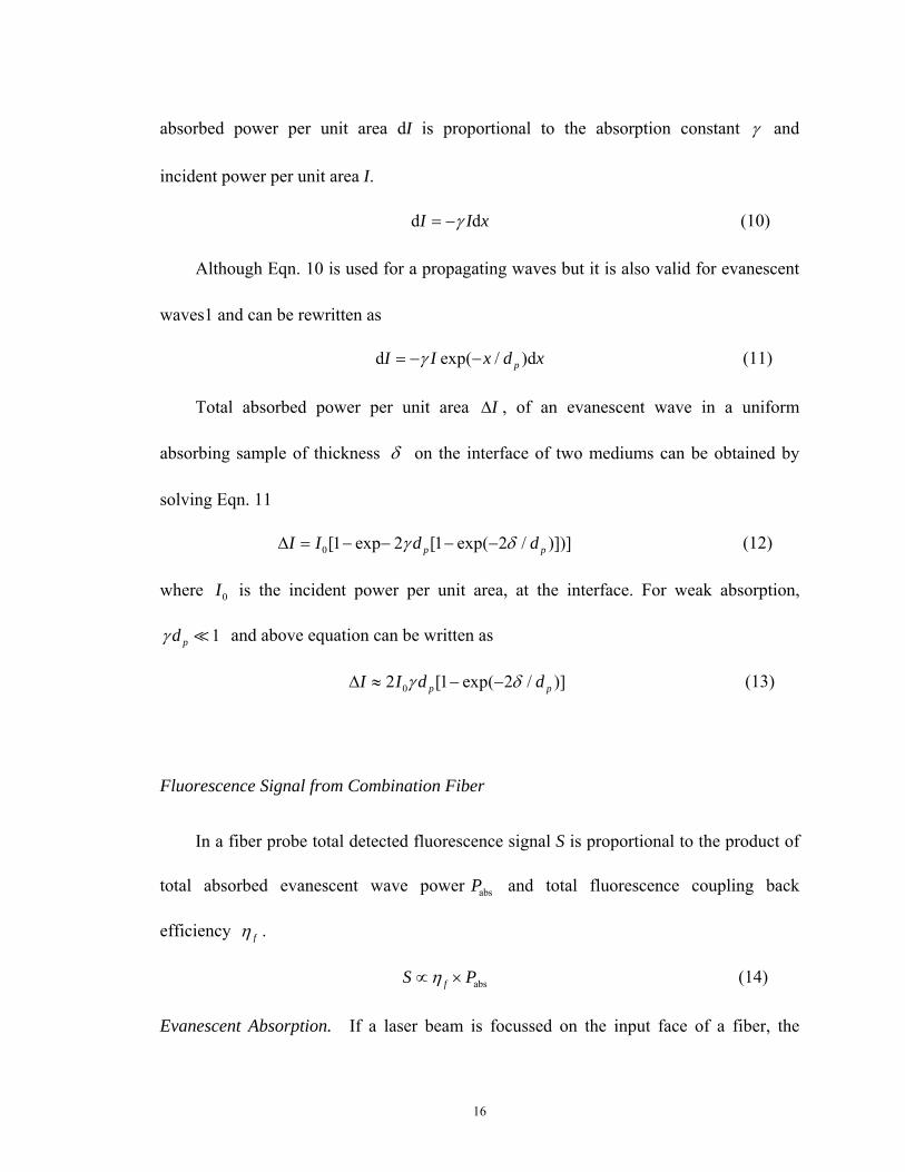
absorbed power per unit area dI is proportional to the absorption constant γ and

incident power per unit area I.

d dI I xγ= − (10)

Although Eqn. 10 is used for a propagating waves but it is also valid for evanescent

waves1 and can be rewritten as

d exp( / )dpI I x d xγ= − − (11)

Total absorbed power per unit area IΔ , of an evanescent wave in a uniform

absorbing sample of thickness δ on the interface of two mediums can be obtained by

solving Eqn. 11

0[1 exp 2 [1 exp( 2 / )])]pI I d d pγ δΔ = − − − − (12)

where 0I is the incident power per unit area, at the interface. For weak absorption,

1pdγ and above equation can be written as

02 [1 exp( 2 /p )]pI I d dγ δΔ ≈ − − (13)

Fluorescence Signal from Combination Fiber

In a fiber probe total detected fluorescence signal S is proportional to the product of

total absorbed evanescent wave power and total fluorescence coupling back

efficiency

absP

fη .

absfS Pη∝ × (14)

Evanescent Absorption. If a laser beam is focussed on the input face of a fiber, the

16

power ray ( )P θ carried by rays between angle θ and dθ θ+ is given as

20

ray 2

2 tan( )sec ( )d( )tan ( )a

PP θ θ θθθ

= (15)

where is the total incident laser power on the fiber surface and 0P aθ is the maximum

acceptance angle of the cladded fiber portion. Love et al.1 have shown that during single

reflection, the absorbed evanescent power of all the rays, making an angle between d aP

θ and dθ θ+ with the central axis of a fiber, in a uniform absorbing medium of

thickness δ on the probe surface is given by

2rel rel

ray 2 2 2rel rel

2 cos 1d ( ) 11 ( 1)cos 1a

n nP Pn n

θθθ

⎡ ⎤−∝ Δ +⎢ ⎥− + −⎣ ⎦

(16)

where is equal to , reln co aq/n n ray ( )P θΔ is power lost to absorbing medium of

thickness δ , by all the rays making an angle between θ and dθ θ+ with the central

axis. As per Eqn. 13 and Eqn. 15 ray ( )P θΔ can be given as

2ray ray co( ) ( ) sin ( ) [1 exp( 2 / )]pP P n d dθ θ θ γ δΔ = − − p (17)

If f is the number of reflections per unit length by a ray making angle θ with the

fiber axis and L is the probe length, the total absorbed evanescent power on the probe

surface can be given as

0abs 2tan a

PPθ

∝

max2

2 2 rel relco 2 2 20 0

rel rel

2 cos 1tan sec sin ( ) [1 exp( 2 / )] 1 d d1 ( 1)cos 1

L

p pn nf n d d

n nθ θ zθ θ θ γ δ

θ⎡ ⎤−

− − +⎢− + −⎣ ⎦∫ ∫ θ⎥

(18)

17

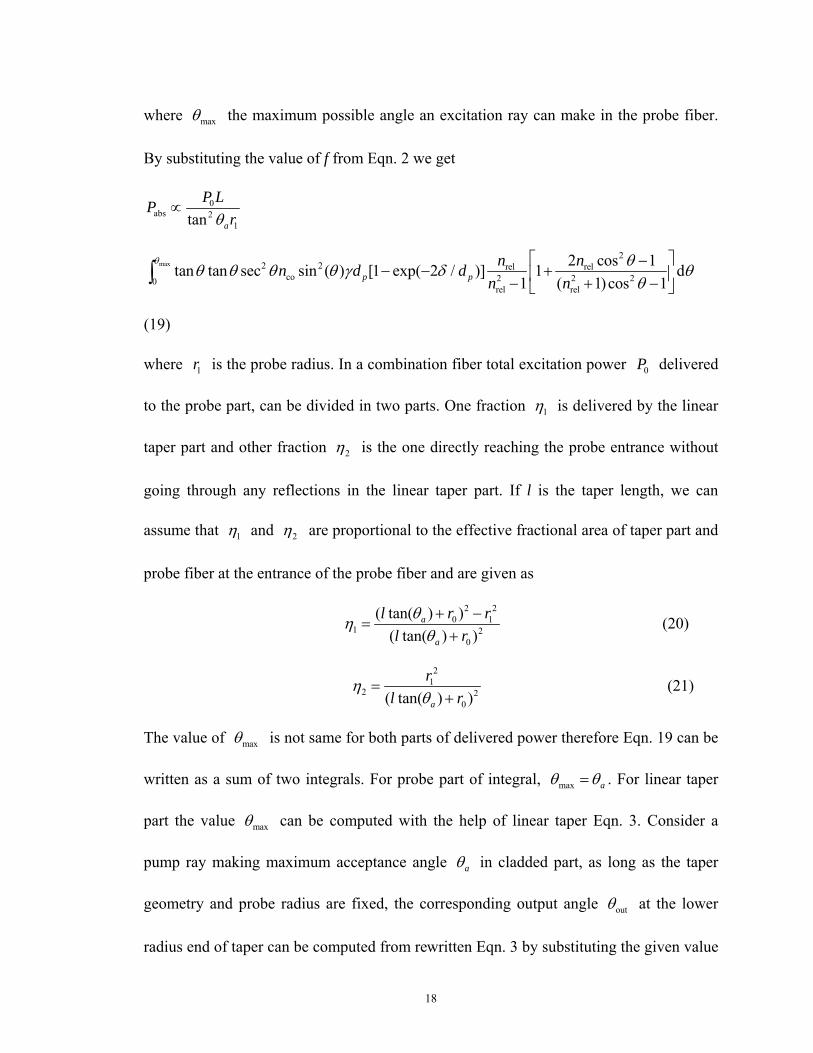
where maxθ the maximum possible angle an excitation ray can make in the probe fiber.

By substituting the value of f from Eqn. 2 we get

0abs 2

1tan a

P LPrθ

∝

max2

2 2 rel relco 2 2 20

rel rel

2 cos 1tan tan sec sin ( ) [1 exp( 2 / )] 1 d1 ( 1)cos 1p p

n nn d dn n

θ θθ θ θ θ γ δθ

θ⎡ ⎤−

− − +⎢ ⎥− + −⎣ ⎦∫

(19)

where is the probe radius. In a combination fiber total excitation power delivered

to the probe part, can be divided in two parts. One fraction

1r 0P

1η is delivered by the linear

taper part and other fraction 2η is the one directly reaching the probe entrance without

going through any reflections in the linear taper part. If l is the taper length, we can

assume that 1η and 2η are proportional to the effective fractional area of taper part and

probe fiber at the entrance of the probe fiber and are given as

2 20 1

1 20

( tan( ) )( tan( ) )

a

a

l rl r

θηθ

r+ −=

+ (20)

21

2 20( tan( ) )a

rl r

ηθ

=+

(21)

The value of maxθ is not same for both parts of delivered power therefore Eqn. 19 can be

written as a sum of two integrals. For probe part of integral, max aθ θ= . For linear taper

part the value maxθ can be computed with the help of linear taper Eqn. 3. Consider a

pump ray making maximum acceptance angle aθ in cladded part, as long as the taper

geometry and probe radius are fixed, the corresponding output angle outθ at the lower

radius end of taper can be computed from rewritten Eqn. 3 by substituting the given value

18

of , and replacing Γ cθ with outθ .

1 0out

1

sin( )sin arr

θθ − ⎡ ⎤= − Γ⎢ ⎥

⎣ ⎦ (22)

Once the value of outθ is know we can set the value of maxθ as

out

max out out

out

0 if 0 if 0

if c

c c

θθ θ θ θ

θ θ θ

<⎧⎪= ≤ ≤⎨⎪ ≥⎩

(23)

Eqn. 19 can be rewritten as

0abs

1

P LPr

∝

max2

2 2 2 rel rel1co2 2 2 20

out rel rel

2 cos 1( tan sec sin ( ) [1 exp( 2 / )] 1 dtan 1 ( 1)cos 1p p

n nn d dn n

θ θη θ θ θ γ δθ θ

θ⎡ ⎤−

− − +⎢ ⎥− + −⎣ ⎦∫

22 2 2 rel rel2

co2 2 2 20rel rel

2 cos 1tan sec sin ( ) [1 exp( 2 / )] 1 d )tan 1 ( 1)cos 1

a

p pa

n nn d dn n

θ θη θ θ θ γ δθ θ

⎡ ⎤−+ − − +⎢ ⎥− + −⎣ ⎦

∫ θ

(24)

Normalization factor 21/ tan ( )aθ in the first integral of Eqn. 24 is replaced with

as the total integral range is taken to be2max1/ tan ( )θ maxθ .

Fluorescence Coupling Back Efficiency. Love et al. (Love 1992) have shown that

fluorescence coupling back efficiency follows the law of reciprocity, therefore fη is

given as

max2 3 2

rel relaq 2 2 20

rel rel

sin ( ) 2 cos 1[1 exp( 2 / )] 1 d1 ( 1)cos 1f p pn nn d d

n nθ θ θη γ δ

θθ

⎡ ⎤−= − − +⎢ ⎥− + −⎣ ⎦

∫ (25)

where the value of maxθ can be computed again with the help of linear taper Eqn. 3.

19

Consider a fluorescence ray making maximum complimentary critical angle cθ in probe

fiber, as long as the taper geometry and probe radius are fixed, the corresponding input

angle inθ at the larger radius end of the linear taper can be computed from rewritten Eqn.

3 by substituting the given value of Γ , and replacing aθ with inθ .

Once the value of inθ is known we can set the value of maxθ as

in outmax

out in out

if if

cθ θ θθ

θ θ θ⎧ ≤

= ⎨>⎩

(26)

Experiments

Probe Preparation

Each probe was an 8 cm long 600 μm core multimode optical fibers (Ocean Optics

Inc.). Approximately 1.5 cm of protective polyimide buffer surrounding the fiber was

removed from one end by burning it with bunsen burner. The fiber was then

decontaminated by sonicating it in a soap solution. This was followed by sonicating the

fiber in a solution of de-ionized water to get rid of any carbon soot on the surface of the

fiber. The cladding of probe part was removed by immersing the 1.5 cm uncoated part

into 5% hydrofluoric acid solution. Probes of various diameters were obtained by

adjusting the time duration of immersion. Tapered part between the etched probe and

cladded fiber was obtained by capillary action. Some acid capillarily ascend into the

space between fiber probe and polyimide buffer. Tapered angle obtained by this method

was found to be nearly constant for all the probes. After taking out of the hydrofluoric

20

acid, the probes were sonicated for four minutes each in deionized water and then in

acetone. The taper angle for each probe was measured using a microscope. The average

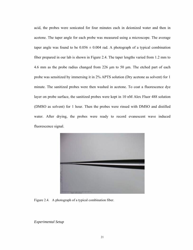
taper angle was found to be 0.056 ± 0.004 rad. A photograph of a typical combination

fiber prepared in our lab is shown in Figure 2.4. The taper lengths varied from 1.2 mm to

4.6 mm as the probe radius changed from 226 μm to 50 μm. The etched part of each

probe was sensitized by immersing it in 2% APTS solution (Dry acetone as solvent) for 1

minute. The sanitized probes were then washed in acetone. To coat a fluorescence dye

layer on probe surface, the sanitized probes were kept in 10 nM Alex Fluor 488 solution

(DMSO as solvent) for 1 hour. Then the probes were rinsed with DMSO and distilled

water. After drying, the probes were ready to record evanescent wave induced

fluorescence signal.

Figure 2.4. A photograph of a typical combination fiber.

Experimental Setup

21

A schematic of our experimental setup is shown in Figure 2.5. A 476 nm laser diode

(Nichia, Japan) was used for excitation. A dichroic band pass filter (476 nm, band width

10 nm) was placed in front of ethanol diode laser to block any red tail emission. The

diode light passes through a dichroic beam combiner/splitter. The beam combiner/splitter

is a short pass filter with high transmission (90%) for the excitation wavelength at 476

nm and high reflectivity (95%) at wavelengths longer than 488 nm. The peak emission

wavelength for Alexa 488 dye is around 530 nm. Laser output is a collimated beam and a

short focal length lens is used to focus the laser beam into a 600 μm core probe fiber. The

evanescent wave induced fluorescence from the probe surface couples back into the

probe fiber and gets transmitted into the collection fiber of a miniature charged coupled

device (CCD) based fiber-optic spectrometer (Ocean Optics Inc., model HR2000). To

further improve the signal to noise ratio, unwanted scattered light from diode laser was

blocked by placing a razor edge 488 nm cut off long pass filter (Edmund Optics Inc) in

front of the collection fiber. This filter has about 95% transmission for all the

wavelengths longer than 500 nm but extremely small transmission (10−6%) for

wavelengths shorter than 500 nm. The signal from the spectrometer is coupled to a

computer (DELL). All the spectra were collected with the help of this computer.

Results and Discussion

Probes of 10 different radii from 50μm to 160μm were prepared. Signal for each

22

probe was recorded in air, water and ethyl alcohol with refractive index 1.0, 1.333 and

1.36 respectively. To further improve the signal to noise ratio, the signal for each probe

was obtained by computing the area under the recorded spectrum curve. It was found that

the observed signal in air reduce by 20-40% when the probe end surface just touch the

water or ethyl alcohol surface, although the full probe length of 1.5 cm was still in air.

This observation was valid for probes of all radii and one plausible explanation for such

observation could be that when the launched light reaches the probe end, it is reflected by

the medium interface. The reflected excitation light will further increase the fluorescence

signal. When air is replaced by water or ethyl alcohol, the Fresnel reflection from the

interface will reduce thus the observed reduction in the signal. But the computed change

in signal by using Fresnel equations show that the contribution of this reflection from a

plane interface will be quite smaller than the observed change. Since our probe end

surface was not a polished surface therefore the back reflection from the rough probe

surface is almost two to three times more. For comparison of results obtained in air with

those in water and ethyl alcohol, the signal recorded in air was corrected for the

experimentally measured scattering factor.

23

Figure 2.5 Experimental setup. LD- Laser Diode, CL- Collimation Lens, BF- Band-pass Filter, ND- Neutral Density filter, LF -Long-pass Filter and SF- Short-pass Filter.

Figure 2.6. Variation of fluorescence signal with probe radius. A comparison of simulation and experimental result.

24

Variation of experimentally recorded fluorescence signal in air, water and ethyl alcohol

as a function of probe radii is shown in Figure 2.6 (scattered points). Simulated

fluorescence signal for different probe radii were also generated. The other parameters

used in this simulation are fiber core radius r 0 = 301μm, fiber core refractive index 1.46,

numerical aperture of fiber 0.22, thickness of absorbing medium on probe surface 0.1 λ

( λ is the excitation laser wavelength), the length of straight probe part was 8 mm

(sensitized region), and the value of taper angle was 0.056 rad. All these probe

parameters were the actual parameters of the probes used for experimental signal

recording. The variation of normalized simulated fluorescence signal in air, water and

ethyl alcohol as a function of probe radii is also shown in Figure 2.6 (solid lines). It can

be seen that the experimentally recorded signals are quite comparable to the simulated

signal.

Conclusions

The results obtained by the simulation are in agreement with experimentally

obtained results. For a given realistic taper length, the maximum signals are obtained at

probe radius smaller than V-number matching radius. In practical conditions it seems

total utilization of excitation light from cladding part to probe zone of a fiber sensor is

difficult to achieve in aqueous environment. Theoretical studies show that taper angle or

taper length, and probing environment play important roles in signal acquisition besides

25

probe radius. Agreement of simulated results with experimental results indicate that the

developed model can provide optimum probe parameters for designing sensor probes in a

given detection environment.

26

REFERENCES

Ahmad, M. and L.L.Hench, "Effect of taper geometries and launch angle on evanescent wave penetration depth in optical fibers," Biosensors and Bioelectronics 20 (7), pp. 1312-1319, 2005.

Anderson, G.P., J.P.Golden, et al, "Development of an evanescent wave fiber optic biosensor." Engineering in Medicine and Biology Magazine, IEEE 13 (3), pp.358-363, 1994.

Axelrod, D., "Total internal reflection fluorescence microscopy," Cell Biology. Tra_c 2, pp.744-764, 2001.

Feynman, R.P., R.B.Leighton and M.Sands, The Feynman Lectures on Physics, 2, 33-6, Addison-Wesley Publishing Company, February, 1997.

Geng, T. M.T.Morgan, and A.K.Bhunia, "Detection of Low Levels of Listeria monocytogenes Cells by Using a Fiber-Optic Immunosensor," Applied and Environmental Microbiology, 70 (10), pp.6138-6146, 2004.

Golden, J.P. G.P.Anderson, S.Y.Rabbany and F.S.Ligler, "An Evanescent Wave Biosensor-Part q: Fluorescent Signal Acquisition from Tapered Fiber Optic Probes," IEEE Transactions on Biomedical Engineering, 41 (6), June 1994.

Kapoor, R., N.Kaur, E.T.Nishanth, S.W.Halvorsen, E.J.Bergey and P.N.Prasad, "Detection of trophic factor activated signaling molecules in cells by a compact fiber-optic sensor," Biosensors and Bioelectronics 20, pp.345-349, 2004.

Ligler, F.S., J.Calvert, J.Georger, L. Shriver-Lake, and S.Bhatia, "A method for attaching functional proteins to silica surface," U.S. Patent 5,077,210, 1991

Love, W.F., L.J.Button, and R.E.Slovacek, "Optical Characteristics of fibreoptic evanescent wave sensors," Biosensors with Fibre Optics, D.L.Wise and L.B.Wingard, Eds., pp.151, Humana Press, Clifton, NJ, 1992.

Marcuse, D., "Launching light into fiber cores from sources in the cladding," J. Lightwave Technol. 6, pp.1273-1279,1988.

Nath, N. and S.Anand,"Evanescent wave fiber optic fluorosensor: effect of tapering configuration on the signal acquistion," Opt.Eng. 37 (1), pp.220-228, January 1998.

27

Snyder, A.W., and J.D.Love, Optical waveguide theory, pp.109, Chapman and Hall, New York, 1983.

Thompson, R.B., L.Kondracki, "Sensitivity enhancement of evanescent wave-excited fiber optic fluorescence sensors," Time resolved laser spectroscopy in biochemistry, II. Proc. IEEE 31, 35-41. 1995.

Willer, U., D.Scheel, I.Kostjucentko, C.Bohling, W.Schade and E.Faber, "Fiber-optic evanescent-field laser sensor for in-situ gas diagnostics," Spectrochim. Acta, Part A 58, pp. 2427-2442, 2002.

28

CHAPTER 3

INTRODUCTION

Backgorund of Magnetic Nanoparticles Usage

Magnetic microspheres and nanoparticles have been used for a variety of

applications and have even been incorporated into medical diagnostic techniques

(Haukanes 1993, Olsvik 1994, Pankhurst 2003, Gijs 2004). Utilizing magnetic particles

coated with antibody to separate target molecules is a widely used separation method

(huang-hao yang and Wang 2004). Besides this, there are a few novel methods proposed

recently aiming at biomolecule detection with magnetic particles.

Weitschies etc. (Weitschies 1997) proposed a novel magnetic relaxation/remanence

immunoassay (MARIA) using a superconducting quantum interference device (SQUID)

(Koelle 1999) as a magnetic field sensor. In the technique, an immobilized target is

immersed in a suspension of superparamagnetic nanoparticles bound to antibodies

specific to that target. A pulsed external magnetic field is applied to align the dipole

moments of the particles. The SQUID detects the magnetic field from the particles bound

to the target. In the presence of this aligning field the nanoparticles develop a net

magnetization, which relaxes when the field is tuned off. Unbound nanoparticles relax

rapidly by Brownian rotation and contribute no measurable signal. Nanoparticles that are

29

bound to the target on the film are immobilized and undergo Neel relaxation2, producing

a slowly decaying magnetic flux, which is detected by the SQUID. (Y. R. Chemla 2000)

McNaughton etc. (Brandon H. McNaughtona 2007; McNaughtona 2007) make use of

shifts in the nonlinear rotational frequency of magnetic microspheres, driven by an

external magnetic field, developed an approach for the detection of single bacterial cells.

At low frequency of the rotating magnetic field, magnetic particles rotates continuously

and synchronously (linear response regime) with the external field. At sufficiently high

external driving frequencies, the particle becomes asynchronous (nonlinear) with the

driving field. When a bacterium attaches to a nonlinearly rotating magnetic microsphere,

the volume and shape of the rotating system are drastically changed, increasing the drag

and thus slowing the rotation rate. The rotational process can be observe and recorded by

standard microscopy equipments.

An interesting method to track the rotation of nano- or microparticles worth

mentioning is the ‘MOONs’ method introduced by Behrend etc (CalebJ. Behrend1 2005).

Coating nanospheres with a metal hemisphere shell breaks the particles’s optical

symmetry, allowing its orientation to be tracked using fluorescence and reflection.

E kN eτ τ=

2 The anisotropy energy barrier of the particle, E, which is proportional to its volume, inhibits the dipole moment from rotating but may be overcome with sufficient thermal energy (T is the temperature and is Boltzmann’s

constant). Thus, Neel relaxation occurs on a time scale , which depends exponentially on the particle volume. In addition to Neel relaxation, nanoparticles in suspension undergo Brownian rotation, which randomizes the orientation of the dipole moments. Typically, for an ideal single-domain, 20-nm magnetic particle

Bk T Bk/

0BT

~ 1N sτ and

~ 1B sτ μ .

30

Fluorescence Polarization Theory

Fluorescence polarization (FP) was first theoretically described by Perrin in 1926

(Perrin 1926); this description was subsequently developed both in theory and

experiment. FP was developed for use in analytical biochemistry, including antigen

(Ag)-antibody (Ab) interactions (Dandliker 1973) and hormone-receptor interactions

(Levison 1976). Quantitative and qualitative measurement of various types of molecules

and bioconjugates has been reported (Wei 1993, Sipior, 1997). In fact, FPI technology has

been applied to several commercially available instruments.

=50ns IgG =150ns

Protein

Fluorophore

φ φ

Figure 3.1. Intuitive illustration of a Fluorescence polarization immunoassay. f is the rotation correlation time.

A FPI requires that emission form the unbound labeled antigen be depolarized, so that

an increase in polarization may be observed upon antigen binding to antibody. For

31

depolarization to occur, the antigen must display a rotational correlation time much shorter

than the lifetime of the probe. The fluorescence life times of various types of fluorophore

ranges from a few nanoseconds to a few microseconds. Among various types of dyes,

long-lifetime fluorophores have an advantage in monitoring binding interaction of

high-molecular-weight antigens, because long-lifetime fluorophores can make the

fluorescence of the labeled high-molecular-weight antigens more depolarized compared to

short lifetime fluorophores. Therefore they are more suitable to be used in FPI except

some fluorophores like Eu3+ and Tb3+ that do not show polarized emission. An intuitive

graph is depicted in Figure 3.1 which illustrates this process.

The fluorescence polarization ( ) of a labeled macromolecule depends on the

fluorescence lifetime (

P

τ ) and the rotational correlation time (φ ):

0

1 1 1 1( ) ( )(13 3P P

)τφ

− = − + , (27)

where is the polarization observed in the absence of rotational diffusion. The

rotational correlation time is related to molecular weight (

0P

rM ) and the molecular volume

of the protein by

(rM v h)RT

ηφ = + , (28)

where R is the ideal gas constant, v is the specific volume of the protein, and is the

hydration. In aqueous solution at 20 C (

h

° 1η = cP) 3, one can expect a protein such as

3 The SI physical unit of dynamic viscosity is the pascal-second (Pa·s), which is identical to 1 kg·m−1·s−1.

The cgs physical unit for dynamic viscosity is the poise (P), named after Jean Louis Marie Poiseuille. It is

32

HSA ( , with 65000rM ≈ 1.9v h+ = ) to display a rotational correlation time near 50 ns.

Polarization is related to the transitional dipole direction of molecules, so reflects the

spatial orientation and rotation dynamics of fluorescent molecules. Another concept

fluorescence anisotropy (FA) is defined as (Lakowicz, 1999)

2I I

rI I

⊥

⊥

−=

+, (29)

where I and I⊥ are fluorescence intensities with polarization parallel and

perpendicular to the excitation polarization, respectively. 2I I⊥+ is the total fluorescence

intensity.

SinceI I

PI I

⊥

⊥

−=

+, the anisotropy and polarization are related by 2

3PrP

=−

, 32

rPr

=+

.

The values of are more often used in FPI because they are entrenched by tradition and

are slightly larger than the anisotropy values. The parameter r is preferred on the basis of

theory.

P

FA can be used to study the rotation diffusion of molecules, which is related to the

size of the molecules and their interactions with the surrounding. In biological studies, FA

measurements have been used to study conformational changes and torsional motion of

the biomolecules and molecular binding interactions (Tramier 2000, Canet 2001).

After being excited by linearly polarized light, polarization of freely rotating more commonly expressed, particularly in ASTM standards, as centipoise (cP). The centipoise is commonly used because water has a viscosity of 1.0020 cP (at 20 °C; the closeness to one is a convenient coincidence). 1 P = 1 g·cm−1·s−1. The relation between poise and pascal-seconds is:10 P = 1 kg·m−1·s−1 = 1 Pa·s;1 cP = 0.001 Pa·s = 1 mPa·s

33

fluorescent molecules decays exponentially during the lifetime of the excited state. When

the polarization of fluorescence can be characterized by fluorescence anisotropy (FA) as

defined in Equ. 29, the temporal average of the time dependent FA function, , is related

to the fluorescence lifetime of the molecules

r

τ . (Dandliker 1973, Terpetschnig 1995)

0

1 /rrτ φ

=+

, (30)

where is the maximum FA without rotational diffusion and 0r φ is the rotational

correlation time of molecules. If the correlation time is much larger than the lifetime

(φ τ ), then the measured anisotropy ( r ) is equal to the fundamental anisotropy ( ). If

the correlation time is much shorter than the lifetime (

0r

φ τ ), then the anisotropy is zero.

is typically near 0.3 for most fluorophores, although the theoretical limit given

collinear transition dipoles for absorption and emission is 0.4.

0r

The expression of is a form of Perrin equation. It can be derived from first

principle based on diffusion steps (Weber 1966). The derivation of this equation begins

with the time-resolved decay of anisotropy for a spherical molecule:

r

( )r t

/ 60 0( ) tr t r e r eφ− −= = /D t , (31)

the rotational correlation time is related to the rotational diffusion coefficient 1(6 )Dφ −= .

Only spherical molecules display single exponential anisotropy decay. Steady-anisotropy

can be calculated from an average of the anisotropy decay by doing integration over time,

which yields the Perrin equation.

According to Stokes-Einstein-Debye equation

34

VkTηφ = , (32)

where η is the viscosity of the solution; is the volume of the molecule; T is the

temperature; is the Boltzmann constant.

V

k φ is a parameter that reflects the rotational

mobility of molecules.

The polarized excitation can also be realized using multi-photons excitation

(Gryczynski 1995), but it is not the issue that will be studied in this thesis.

Some Explanations of Anisotropy Theory

Calculation of Rotational Correlation Time of Proteins

For globular proteins the rotational correlation time is approximately related to the

molecular weight ( M ) of the protein by

(V M v h)RT RTη ηφ = = + (33)

where is the molar volume after hydration, V v is the specific volume of the protein,

and is the hydration, T is the temperature in K, h ° 78.31 10 erg/mol KR = × ° , and the

viscosity η is in poise ( ). Values of for proteins are typically near 0.73 ml/g, and

the hydration is near 0.23 g per gram of protein. This expression predicts that the

correlation time of a hydrated protein is about 30% larger than that expected for an

anhydrous sphere. Generally, the observed values of rotational correlation time are about

twice that expected for an anhydrous sphere (Yguerabide, 1970).

P h

2H O

For example, for anhydrous protein sphere with a 10 kD molecular weight, with

35

0ml/gh = and =1cP=0.01Pη , 0.75ml/gv = , then the value of rotational correlation

time can be calculated as

3

7

0.01 10 10 g / mol 0.75ml/g 3.1ns8.31 10 erg/(mol K) 293 K

Pφ × × ×= ≈

× ° × °i

The expected anisotropy values for a range of photoluminescence lifetimes are

simulated in Figure 3.2. The calculations were based on the assumption that the limiting

anisotropy in the absence of rotational diffusion, the solution viscosity was 1cP,

and

0 0.3r =

v h+ =1.9ml/g for the protein.

103 104 105 106 107 1080

0.05

0.1

0.15

0.2

0.25

0.3

0.35

Molecular Weight (Daltons)

Ani

sotro

py

5 ns

50 ns

1 us

3us

Figure 3.2. Molecular-weight-dependent anisotropy for a protein-bound luminophore with luminescence lifetimes of 5, 50, 1000, and 3000 ns. The curves are based on assumption that the

aqueous solution is at 20 C with a viscosity of 1 cP and ° v h+ =1.9ml/g.

36

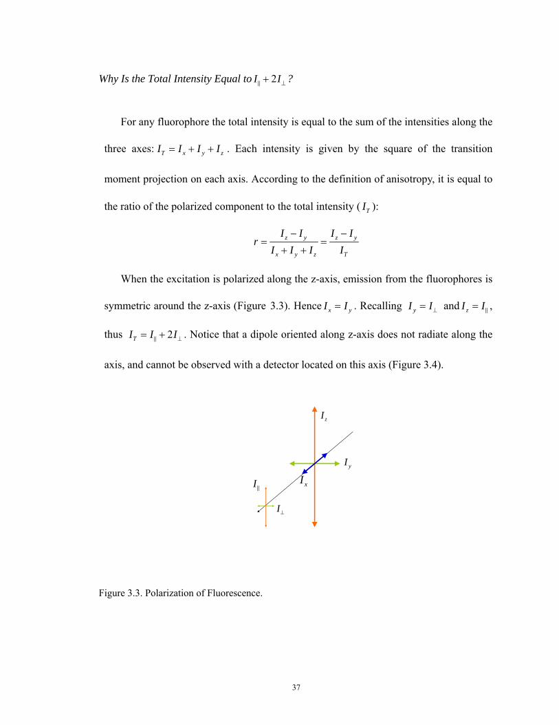
Why Is the Total Intensity Equal to I I2 ⊥+

z

?

For any fluorophore the total intensity is equal to the sum of the intensities along the

three axes: T x yI I I I= + + . Each intensity is given by the square of the transition

moment projection on each axis. According to the definition of anisotropy, it is equal to

the ratio of the polarized component to the total intensity ( TI ):

z y z y

x y z T

I I Ir

II I I I

− −= =

+ +

When the excitation is polarized along the z-axis, emission from the fluorophores is

symmetric around the z-axis (Figure 3.3). Hence x yI I= . Recalling yI I⊥= and zI I= ,

thus 2TI I I⊥= + . Notice that a dipole oriented along z-axis does not radiate along the

axis, and cannot be observed with a detector located on this axis (Figure 3.4).

I

I⊥

yI

zI

xI

Figure 3.3. Polarization of Fluorescence.

37

Figure 3.4. Dipole radiation pattern

CHAPTER 4

NOVEL IDEA INTRODUCED TO FPI

Before Terpetschniq etc. discovered a Ruthenium complex dye that displays

polarized emission and has a lifetime of about 400 ns, a limitation exists in the

immunoassay using FPI. The lifetimes of Fluorophores used were usually very short. For

example, fluorescein, displays a lifetime near 4 ns. A FPI requires that emission from the

unbound labeled antigen be depolarized, so that an increase in polarization may be

observed upon antigen binding to antibody. For depolarization to occur, the antigen must

display a rotational correlation time much shorter than the lifetime of the probe. Short

fluorophore life time will limit the dynamic range of FPI for antigens with low molecular

weights (Figure 3.2)

Guo etc. (Guo, Castellano et al. 1998) developed a FPI based on luminescence from

38

a Re(I) metal-ligand complex which has a lifetime of 2.7 μs. This long-lifetime dye

enhanced the potential of FPI to detect antigens with molecular weight above 107 Daltons

in theory.

While long-lifetime dye provides a possibility to FPI measurement for large

molecular weight antigens, for very large molecular weight antigens, above 106 Daltons

for example, the small dynamic range problem still exist, and the same problem with the

detection of very small molecular weight proteins. After antibody binding of small

molecular weight protein, the total weight of antigen and antibody usually do not exceed

106 Daltons, and the eventual anisotropy will not be greater than 0.1 with fluorophore

lifetime of 3 μs according to Figure 3.2., which is a theoretical simulation and the

detailed procedures are described later.

To solve the above problems, a novel method is proposed in this study that uses

antibody coated magnetic nanoparticles instead of antibody to do the FPI measurements.

Since the nanoparticles usually consist of iron oxide, each particle has a much greater

weight than a single antibody. When they are coated with antibody, and the

immunoreaction take place, the binding will generate a dragging effect and significantly

change the rotation correlation time of antigens. By FPI measurement, the utilization of

magnetic nanoparticles can result in a more appreciable anisotropy change. Further more,

by applying a DC magnetic field on the sample, the magnetic dipole moments of

nanoparticles are aligned in the same direction, inhibiting thermal agitation and rotation,

thus can further enhance the anisotropy change. Even when the dynamic range of

39

anisotropy change has already been small for the antigens with molecular weight greater

than a certain level, the anisotropy change can be modulated using a step-down magnetic

field with an appropriate frequency. The modulated anisotropy change, though small and

may not be appreciable, can be picked out by lock-in amplifier.

The advantages of this FPI method using antibody-coated magnetic nanoparticles are

that it becomes feasible to perform FPI on a wide range of antigens with different

molecular weights using a single type of fluorophore, and enhance the dynamic range of

anisotropy change, which results in more precise immunoassay.

The magnetic particles used should be superparamagnetic particles. Compare to

paramagnetic particles, superparamagnetic particles usually have smaller dimensions.

Because of the small scale of superparamagnetic particles, the ambient thermal energy is

sufficient to change the direction of magnetic moment of a particle. The random rotation

of particles will cause a certain extent of depolarization of fluorescence, which is an

essential condition in order to observe the anisotropy change after applying the magnetic

field.

40

CHAPTER 5

KNOWLEDGE OF MAGNETISM FOR DETERMING SUITABLE NANOPARTICLES TO BE USED

It would be useful to clarify some concepts in magnetism before getting into the part

of type selection of magnetic particles.

Definitions and Units

There are three magnetic vectors: H, Magnetic field; M, Magnetization; B, Magnetic

induction.

A magnetic field H will be produced at the center of a current loop given by

2iHr

= [Amperes/meter, A/m]

The current loop has a magnetic moment, m, associated with it

Aream i= × [Am2]

The intensity of magnetization, M, is magnetic moment per unit volume

/M m V= [A/m]

Susceptibility is the ratio of magnetization to magnetic field, /k M H=

[dimensionless].

In SI system, the relationship between B , H and M is given by 0 ( )B H Mμ= +

constant 0[Tesla, T]. The μ is called the rmeability of free space. In SI it is equal

to 74 10 Henπ −×

pe

ry/m .

41

In CGS, 0μ is set equal to unity, which makes the relation among the three vectors

to be 4B H Mπ= + , but each have a different unit name, i.e. Gauss for B , Oersted for

H , and emu/cm3 for M .

Some units conversions between SI and CGS are listed in the Table 5-1. It should be

noted that when talking about a magnetic “field” of 100 milliTesla (mT) in some cases

that are not very rigorous, it really means 0 100mTHμ = .

Table 5-1 Magnetic units.

Magnetic Term Symbol SI unit CGS unit conversion factor magnetic induction B Tesla (T) Gauss (G) 1 T = 104 G magnetic field H A/m Oersted (Oe) 1 A/m =4π/103 Oe magnetization M A/m emu/cm3 1 A/m = 10-3 emu/cm3

magnetic moment m Am2 emu 1 Am2 = 103emu permeability of free space

μ0 H/m dimensionless 4πx10-7 H/m = 1 (cgs)

Classes of Magnetic Materials

The origin of magnetism lies in the orbital and spin motions of electrons and how

the electrons interact with one another. It can be classified by different ways materials

respond to magnetic fields.

The five major groups are diamagnetism, paramagnetism, ferromagnetism,

ferrimagnetism, and antiferromagnetism. Materials in the first two groups are those that

exhibit no collective magnetic interactions and are not magnetically ordered. Materials in

the last three groups exhibit long-range magnetic order below a certain critical

42

temperature. Besides the above five categories, a particular

magnetism-superparamagnetism interests us most, because only magnetic particles in

nano-scale have the possibility of showing superparamagnetic characteristics.

Diamagnetism

Diamagnetism is a fundamental property of all matter, although it is usually very

weak. It is due to the non-cooperative behavior of orbiting electrons when exposed to an

applied magnetic field. Diamagnetic substances are composed of atoms which have no

net magnetic moments (i.e., all the orbital shells are filled and there are no unpaired

electrons).

Paramagnetism

As for this class of materials, some of the atoms or ions in the material have a net

magnetic moment due to unpaired electrons in partially filled orbitals. However, the

individual magnetic moments do not interact magnetically, and like diamagnetism, the

magnetization is zero when the field is removed. In the presence of a field, there is now a

partial alignment of the atomic magnetic moments in the direction of the field, resulting

in a net positive magnetization and positive susceptibility.

In addition, the efficiency of the field in aligning the moments is opposed by the

randomizing effects of temperature. This results in a temperature dependent susceptibility,

43

known as the Curie Law.4

At normal temperatures and in moderate fields, the paramagnetic susceptibility is

small (but larger than the diamagnetic contribution). Unless the temperature is very low

(<<100 K) or the field is very high paramagnetic susceptibility is independent of the

applied field. Under these conditions, paramagnetic susceptibility is proportional to the

total iron content.

Ferromagnetism

Unlike paramagnetic materials, the atomic moments in ferromagnetic materials

exhibit very strong interactions. These interactions are produced by electronic exchange

forces and result in a parallel or antiparallel alignment of atomic moments. Exchange

forces are very large, equivalent to a field on the order of 1000 Tesla, or approximately a

100 million times the strength of the earth's field.

The exchange force is a quantum mechanical phenomenon due to the relative

orientation of the spins of two electrons.

Ferromagnetic materials exhibit parallel alignment of moments resulting in large net

magnetization even in the absence of a magnetic field. The elements Fe, Ni, and Co and

many of their alloys are typical ferromagnetic materials.

4 Curie's law For low levels of magnetisation, the magnetisation of paramagnets follows Curie's law to

good approximation:BM B CT

χ= =i i , where M is the resulting magnetization, B is the magnetic flux

density of the applied field, measured in teslas, T is absolute temperature, measured in kelvins, C is a material-specific Curie constant

44

There is a big difference between paramagnetic and ferromagnetic susceptibility. As

compared to paramagnetic materials, the magnetization in ferromagnetic materials is

saturated in moderate magnetic fields and at high (room-temperature) temperatures:

Table 5-2 Differences between paramagnetism and ferromagnetism.

Hsat (T) T range (K) χ 10-8m3/kg

paramagnetis >10 <<100 ~50

ferromagnets ~1 ~300 1000-10000

Ferrimagnetism

In ionic compounds, such as oxides, more complex forms of magnetic ordering can

occur as a result of the crystal structure. One type of magnetic ordering is called

ferrimagnetism. The magnetic structure is composed of two magnetic sublattices (called

A and B) separated by oxygens. The exchange interactions are mediated by the oxygen

anions. When this happens, the interactions are called indirect or superexchange

interactions. The strongest superexchange interactions result in an antiparallel alignment

of spins between the A and B sublattice. In ferrimagnets, the magnetic moments of the A

and B sublattices are not equal and result in a net magnetic moment. Ferrimagnetism is

therefore similar to ferromagnetism.

Antiferromagnetism

45

If the A and B sublattice moments are exactly equal but opposite, the net moment is

zero. This type of magnetic ordering is called antiferromagnetism.

Superparamagnetism.

There are materials that show induced magnetic behavior that follows a Curie type

law but with exceptionally large values for the Curie constants. These materials are

known as superparamagnets. They are characterized by a strong ferro- or ferrimagnetic

type of coupling into domains of a limited size that behave independently from one

another.

Superparamagnetism is a small length-scale phenomenon, where the energy

required to change the direction of the magnetic moment of a particle is comparable to

the ambient thermal energy. At this point, the rate at which the particles will randomly

reverse direction becomes significant (Kryder 2005).

Normally, coupling forces in ferromagnetic materials cause the magnetic moments of

neighboring atoms to align, resulting in very large internal magnetic field. This is what

distinguishes ferromagnetic materials from paramagnetic materials. At temperatures

above the Curie temperature (or the Neel temperature for antiferromagnetic materials), the

thermal energy is sufficient to overcome the coupling forces, causing the atomic magnetic

moments to fluctuate randomly. Because there is no longer any magnetic order, the internal

magnetic field no longer exists and the material exhibits paramagnetic behavior. If the

46

material is non-homogeneous, one can observe a mixture of ferromagnetic and

paramagnetic clusters of atoms at the same temperature, the superparamagnetic stage.

Superparamagnetism occurs when the material is composed of very small crystallites

(1–10 nm). In this case even when the temperature is below the Curie or Neel temperature

(and hence the thermal energy is not sufficient to overcome the coupling forces between

neighboring atoms), the thermal energy is sufficient to change the direction of

magnetization of the entire crystallite. The resulting fluctuations in the direction of

magnetization cause the magnetic field to average to zero. Thus the material behaves in a

manner similar to paramagnetism, except that instead of each individual atom being

independently influenced by an external magnetic field, the magnetic moment of the

entire crystallite tends to align with the magnetic field.

The energy required to change the direction of magnetization of a crystallite is called

the crystalline anisotropy energy and depends both on the material properties and the

crystallite size. As the crystallite size decreases, so does the crystalline anisotropy energy,

resulting in a decrease in the temperature at which the material becomes

superparamagnetic.

The differences among ferromagnetism, paramagnetism and superparamagnetism

can be summarized as that: atoms of ferromagnetism have parallel aligned magnetic

moments, atoms of paramagnetism have randomly oriented magnetic moments with the

absence of magnetic field, while atoms of superparamagnetism only have aligned

47

magnetic moments in a small single domain, in a crystallite for example.

What Kind of Magnetic Particles Are Suitable for This Purpose?

According to the description from the last section, ferromagnetic nanoparticles and

superparamagnetic nanoparticles can meet the requirement of FPI. Because these kinds

of particles are apt to be agitated by ambient thermal energy so that they can provide the

depolarization condition before applying a magnetic field to modulate the FP change. To

determine the particle sizes that are suitable for FPI, let us start with the two magnetic

relaxations of particles, that are characterized by the sized of particles.

After switching off the magnetic field that has aligned nanoparticles (MNPs), the

magnetization of MNPs can relax either through Brownian or through a Neel relaxation

mechanism. If the MNP is suspended in a liquid and if the magnetic anisotropy constant

of the MNP is high enough to block the magnetization inside the MNP, then the MNP can

undergo Brownian rotation which randomizes the orientation of the dipole moments. If

the magnetization is unblocked, the internally-Neel relaxation occurs (Ludwig 2004).

The dominant relaxation process for MNPs suspended in a liquid depends on the

particle size. The time constant of Brownian relaxation is given by B 3 /V k TBτ η= , where

is the hydrodynamic volume of the MNP, V η is the viscosity of the carrier liquid,

the Boltzman constant and the temperature. The time constant of Neel relaxation is

given by

Bk

T

N 0 Bexp( / )KV k Tτ τ= , where 0τ is usually taken as 10-9s, K is the magnetic

48

anisotropy5 constant and the volume of the MNP. The calculated relaxation times of

Brownian and Neel relaxation are depicted in Figure 5.1 and 5.2.

V

10 20 30 40 50 60 70 80 90 1000

50

100

150

200

250

300

350

400

Nanoparticle Diameter (nm)

Bro

wni

an R

elax

atio

n Ti

me

( μs)

Figure 5.1. Brownian relaxation time versus MNP diameter. T=300 K.

5 6 7 8 9 10 11 12 13 14 15 160

0.5

1

1.5

2

2.5

3

3.5

4

4.5

5

Nanoparticle Diameter (nm)

Rel

axat

ion

Tim

e ( μ

s)

τBrow nian

τNeel

Figure 5.2. Relaxation times of Brownian and Neel relaxation versus MNP core diameter. K=20 kJ/m3 and T=300 K were assumed.

5 Magnetic anisotropy is the direction dependence of a material’s magnetic properties. A magnetically isotropic material has no preferential direction for its magnetic moment is zero field, while a magnetically anisotropic material will align its moment to an easy axis.

49

Figure 5.2 indicates that there are different scenarios that can be used for the specific

detection of biomolecules according to characteristics of Brownian and Neel relaxation.

If the MNPs are immobilized by their binding to a specific biomolecules and if they have

a suitable size, they exhibit Neel relaxation whereas unbound ones relax via Brownian

rotation. In this way, bound and unbound MNPs can be clearly distinguished by their

different relaxation times. If the MNP binds to a biomolecule, both being in suspension

and consequently mobile, its hydrodynamic volume will be increased, resulting in an

increased Brownian time constant, dependent on whether it exceeds the corresponding

Neel time constant or not (Ludwig 2004).

In the study of FPI using magnetic nanoparticles, what we concern most is the

Brownian relaxation time. Because FPI is performed in liquid environment, and all the

particles are mobile and not immobilized to some sites. Moreover, in the expression of

fluorescence anisotropy, the rotational correlation time is actually Brownian relaxation

time accrording to their respective formula.

Since the dye lifetimes usually do not exceed a few microseconds level, according to

Figure 3.2 and 5.1, the nanoparticles can be used in FPI should be only a few tens of

nanometers in size. If the nanoparticles are too big, for one thing, the correlation time

becomes very long and may not be comparable with the fluorescence lifetime, and the

fluorescence anisotropy change would be very difficult to pick out by measuring

equipment. For another, large particles are apt to settle down in testing container, thus

cannot meet the requirement that the particles should be easy to be suspended in liquid for

50

some time to perform the FPI.

Possibility to Extract the Signal

After immuno-reaction, assume the nanoparticles attached with antigens have a

correlation time of 100 μs, and the dye used has a lifetime of 1μs, then according to Equ.

30. the fluorescence lifetime is

0 0.3 0.29701 / 1 1/100

rrτ φ

= = =+ +

.

After applying magnetic field, particles are all aligned. The particles can be seen to be

immobilized and there is no Brownian relaxation happen. Thus the rotational correlation

time can be deemed as infinity, and the anisotropy has the assumed maximum value 0.3

here. The anisotropy change is 0.003. According to experimental measurement, the

anisotropy fluctuation is usually within 0.01, so the anisotropy change after applying

magnetic field cannot be observed directly. However, if a modulated magnetic field is

utilized, then the anisotropy change signal that is buried in noise can be pick out by a

lock-in amplifier.

Commercial Sources of Dye and Magnetic Nanoparticles

Long lifetime dye of around 1 μs or longer is required in this proposed method. A

commercial available ruthenium complex dye Fluka 71603 can be obtained from

Sigma-Aldrich Inc. Its synonym is Ru(bpy)2(phen-5-isothiocyanate)(PF6)2,, with

51

molecular formula C33H23F12N7P2RuS. Its labeling process is quite easy and it can yield a

high dye-to-protein labeling ratio (Szmacinski 1996).

Clemente Associates provides iron oxide magnetic nanoparticles with diameter

around 50 nm. Those particles are pre-coated with antibodies or activechemicals.They

also provide special order of particles with diameter around 35nm.

52

CHAPTER 6

EXPERIMENTAL PART

Magnetic Field Construction Strategy

To align the magnetic nanoparticles, a uniform and steady DC magnetic field is

needed. A normal solenoid can generate this uniform magnetic field, but the analyte is

required to be placed in the center of the solenoid, which is very difficult with the

involvement of optical setup. In this case, a pair of helmholtz coils is a good choice since

it will not block the optical paths in neither excitation nor detection besides excellent

homogeneous characteristic of magnetic field it generates.

A helmholtz coil pair is made up of two, identical, circular coils aligned on the same

axis and separated by a particular distance. This separation distance, which is equal to the

radius of the coil, is the feature that makes the mixing process of immunoassay easy to

achieve. A simple calculation gives the correct value of the field at the center point. If the

radius is R , the number of turns in each coil is and the current flowing through the

coils is

N

I , then the magnetic flux density, B at the midpoint between the coils will be

given by,

1.5 00.8 ,NIBR

μ=

where 0μ is the permeability constant . 74 10 T m/Aπ −× i

In the case of this research, the sample which is contained in a cuvette needs to be

53

place in the optical testing cube, which can prevent the material from the outer

background light. A rectangular pair of helmholtz coil design is introduced in this

magnetic field construction, because it have the following advantages:

(1) Ease of construction of the coil forms,

(2) Ease of alignment of the coils by making use of the optical testing cube, and

(3) Relative ease of field computations.

Figure 6.1. Magnetic field calculation of a segment of straight wire carrying current.

According to Biot-Savart Law (Preston 1991, Tipler 1999), if the differential element of

current is defined as Idl , then the corresponding differential element of magnetic field is,

024

Idl rd Br

μπ

×= ， (34)

integrate this differential element along the straight wire segment as shown in Figure 6.1.

The magnitude of magnetic field at a point that has a distance s away from the wire

segment can be easily obtained as,

54

0 1 (cos cos )4

IBs

μ α βπ

= −i , (35)

where α and β are the angles shown in Figure 6.1.

The fields generated by a pair of rectangular coils can be easily derived by summing

the contribution of each of the eight line segments of current. In this manner one can

obtain an explicit expression for the field at any point without the use of elliptic integrals.

Computer programs were developed to plot contours of the axial field deviation using

MATLAB (Appendix B).

Figure 6.2. Cartesian coordinate system for the rectangular helmholtz coils.

The coordinate system used in the field plots, are Cartesian coordinate system (x, y,

z) as shown in Figure 6.2. The x and y axes are parallel to the coil sides and z axis is

perpendicular to the coil planes and passes through their centers. The coils used in this

computation are that with width of 6cm, height of 6.5 cm and distance of 5 cm between

55

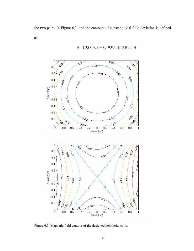
the two pairs. In Figure 6.3, and the contours of constant axial field deviation is defined

as:

[ ( , , ) (0,0,0)] / (0,0,0)z z zB x y z B BΔ = −

Figure 6.3. Magnetic field contour of the designed helmholtz coils.

56

It can be seen from the contour graph that within the volume of cube located

at the origin, the deviation of magnetic field is less than 2%. The field in gauss at the

center of the pair of rectangular coils helmholtz coils, , is given by,

31cm

(0,0,0)zB

(0,0,0) 0.19199zB NI= ,

where N is the number of turns on each coil, I the current in amperes.

A pair of plastic spools was manufactured to hold the rectangular helmholtz coils.

They can be mounted on both sides of the optical testing cube as shown in Figure 6.4.

Mounting spools on the cube provides an advantage that the coils don’t need stands to

hold them and the alignment of the two coils are automatically achieved.

Figure 6.0.4. Mounting spools onto testing cube (not to scale).

The dimensioned drawings of the spools are shown in Figure 6.4.

57

Figure 6.5. Coil spools design scheme.

DC Magnetic Field Construction and Calibration

The pair of spools was mounted on both sides of the testing tube, on each of which

wounded 100 rounds of enameled copper magnet wire (WLS85135-40J, Sargent-Welch).

The two spools of coil were connected in series and formed a close circuit by connecting

them to anode and cathode of a power supply (CP32787-00, Sargent-Welch). A Gauss

meter (GM1A, Applied Magnetics Laboratory Inc.) with transverse probe was used to

detect the magnetic induction B by placing the probe in the testing tube and facing the

probe flake parallel to the magnetic field. When performing the calibration, a multi-meter

was connected in the circuit in series to measure the circuit current. After increasing the

current the a certain value, it is decreased to observe if there is big hysteresis. The

58

magnetic field in the center of testing tube versus magnetic current is listed in Table 6-1.

Table 6-1 Magnetic field versus current.

Current (A) Magnetic Field (Gauss)

1/3 13.0

2/3 21.4

1 28.8

2/3 22.3

1/3 13.4

The measured data shows the magnetic field at current 2/3 A which was used in later

designed Fluorescence Polarization experiment varies only about 0.04%, so it can

provide an acceptably stable magnetic field.

Optical Setup

The whole experimental setup scheme is illustrated in Figure 6.6. A 405 nm laser

diode (Nicha, Japan) controlled by a Laser diode controller (LDC 202C, Thorlabs) was

used to generate excitation laser. After passing through a Glan-Thompson Polarizer to

make the laser vertically polarized, the laser was reflected by a long pass filter in the

59

direction of where sample was placed. A short focal length lens mounted on a position

tunable adapter was used to focus the laser in sample. Fluorescence generated by

excitation of the laser was detected by the detection part of the system which mainly

consisted of a Glan-Taylor polarizer and two CCDs (MiniSpectrometer, Hamamatsu;

HR2000+, OceanOptics). The Glan-Taylor polarizer (GT10-A, Thorlabs) split the two

polarization components of the fluorescence and directed each of them to a CCD by a

lens (F220SMA-A, Thorlabs) and a piece of optical fiber. The spectrum were displayed

and recorded in two software environments.

LDC

LDGlan-Thompson Polarizer

Optical Fiber CCD1

CCD2

Computer

Current Supply

HelmholtzCoils

Sample

LongpassFilter

Glan-Taylor Polarizer

Figure 6.6. Experimental setup of Fluorescence Polarization.

Glan-Thompson Polarizer

60

The extinction ratio6 of Glan Thompson calcite polarizers (Figure 6.7) can reach up

to 100,000:1. The polarizer consists of two cemented prisms made from the highest

optical grade calcite. The operating spectral range is 350 nm to 2.3 μm.

Figure 6.7. Glan Thomson Polarizer. A Glan-Thompson prism deflects the p-polarized ordinary ray whilst transmitting the s-polarized extraordinary ray. The two halves of the prism are joined with optical cement, and the crystal axes are perpendicular to the plane of the diagram.

A Glan-Thompson prism consists of two right-angled calcite prisms that are

cemented together by their long faces. The optical axes of the calcite crystals are parallel

and aligned perpendicular to the plane of reflection. Birefringence splits light entering

the prism into two rays, experiencing different refractive indices; the p-polarized o-ray is

totally internally reflected from the calcite-cement interface, leaving the s-polarized e-ray

to be transmitted. The prism can therefore be used as a polarizing beam splitter.

Traditionally Canada balsam was used as the cement in assembling these prisms.

The Glan-Thompson has a wide acceptance angle, but a much lower limit of

maximum irradiance (due to optical damage limitations of the cement layer).

6 Extinction Ratio is a measure of the ability of a polarizer to attenuate plane polarized light. The extinction ratio can be calculated by measuring the ratio of the maximum transmission(Tmax) when the polarizer is aligned to the poarization axis and the minimum transmission (Tmin) when the poarizer is rotate 90 degrees. The ratio ER = Tmax/Tmin is often expressed in a form like 1000:1

61

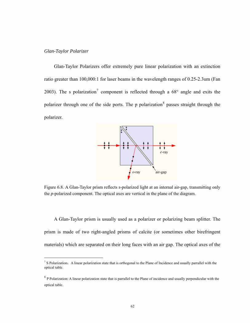
Glan-Taylor Polarizer

Glan-Taylor Polarizers offer extremely pure linear polarization with an extinction

ratio greater than 100,000:1 for laser beams in the wavelength ranges of 0.25-2.3um (Fan

2003). The s polarization7 component is reflected through a 68° angle and exits the

polarizer through one of the side ports. The p polarization8 passes straight through the

polarizer.

Figure 6.8. A Glan-Taylor prism reflects s-polarized light at an internal air-gap, transmitting only the p-polarized component. The optical axes are vertical in the plane of the diagram.

A Glan-Taylor prism is usually used as a polarizer or polarizing beam splitter. The

prism is made of two right-angled prisms of calcite (or sometimes other birefringent

materials) which are separated on their long faces with an air gap. The optical axes of the

7 S Polarization：A linear polarization state that is orthogonal to the Plane of Incidence and usually parrallel with the optical table.

8 P Polarization: A linear polarization state that is parrallel to the Plane of incidence and usually perpendicular with the

optical table.

62

calcite crystals are aligned parallel to the plane of reflection. Total internal reflection of

s-polarized light at the air-gap ensures that only p-polarized light is transmitted by the

device. Because the angle of incidence at the gap can be reasonably close to Brewster's

angle, unwanted reflection of p polarized light is reduced, giving the Glan-Taylor prism

very good transmission.

63

CHAPTER 7

FA Meaurement and Data Processing

From the fluorescence components of parallel and perpendicular polarizations, FA

can be calculated using the equation

2

I Ir

I I⊥

⊥

−=

+, (36)

where I and I⊥ are the fluorescence intensities with polarization parallel and

perpendicular to the excitation polarization, respectively.

However, optical components may have different transmission efficiency for the

two polarization components and the two detectors my also have different sensitivities.

Even for a particular detector, it may have different sensitivities to different polarizations.

This point can be illustrated by the following experiment: A 405nm vertically polarized

laser was launched into the optical system, 99ul PBS and 1ul 1mg/ml Alex Fluor 430

labeled BSA were mixed together to serve as the testing sample. The fluorescence

generated has a peak at 546.35nm. Hamamatsu spectrometer was used to detect the s

(horizontal) polarized light while OceanOptics spectrometer was used to detect the p

(vertical) polarized light. The intensity counts in the two spectrometers at wavelength

546.35nm were recorded for three times respectively. Then the fiber connectors at the

two spectrometers were exchanged so that OceanOptics spectrometer was used to

measure the s polarized light and Hamamatsu p polarized light. The results are shown in

64

Table 7-1.

Table 7-1 Comparison on sensitivity of two spectrometers to polarized light

1 2 3 Average Hamamatsu_s 7339 7095 6935 7123 OceanOptics_p 11735 11067 10798 11200

Hamamatsu_p 12406 11482 11799 11895.67 OceanOptics_s 9872 9027 9254 9384.333

It can be seen that for s polarized light, OceanOptics Spectrometer has a higher

sensitivity while for p polarized light, Hamamatsu gives greater intensity counts.

Effects of these differences are usually taken into account by a correction factor G

(Siegel 2003), which is the ratio of efficiencies for the parallel and perpendicular

detection channels. can be determined experimentally once the optical path is set and

well aligned. To determine theG , a method was developed as follows: For vertically

polarized excitation, the paralleled fluorescence component is polarized and detected

by CCD1 as

G

p

vvI , while the perpendicular fluorescence component detected as vhI is

polarized. Using and to represent the combined transmission and detection

efficiencies for and polarization detecting channels, relations can be obtained as

s

vS hS

p s

,vv vI S I=

vh hI S I⊥= ,

If is the ratio between and , then G vS hS

65

1h vv vv

v vh vh

I S I II S I G I⊥

= = .

For horizontally polarized excitation, the parallel fluorescence component I is

polarized and detected by CCD2 as

s

hhI , while the polarized fluorescence component

detected by CCD1 as

p

hvI is vertically polarized. Similarly,

v hh hh

h hv hv

I S I IGI S I I⊥

= =

According to the above two equation,

vv hv

vh hh

I IGI I

= . (37)

Since h vv

v vh

I S II S I⊥

= , then

2h vv v vh

h vv v vh

S I S IrS I S I

−=

+ (38)

After dividing the nominator and denominator both by , equation (1) can be modified

to

hS

2

vv vh

vv vh

I GIrI GI

−=

+. (39)

It can also be written in the horizontal polarized excitation form. Therefore, before the

FA measurement, the G factor needs to be determined by making horizontal and

vertical polarized excitation measurement respectively. After the value of G is

determined by Equ. 37, it should be applied to each measurement to get the anisotropy

value. And the ensuing measurement can be made only with vertical polarized excitation

light which is suitable for the current optical setting, because the vertical polarized light

66

gives stronger signal due to different polarization reflectivity of the filter to the excitation

light.

67

CHAPTER 8

RESULTS AND DISCUSSIONS

Determine the G Factor

1μl Alex Fluor 430 labeled BSA was mixed into 99 ul PBS. The polarization

components were recorded three times with vertically polarized excitation and

horizontally polarized excitation respectively.

Table 8-1 Measurements for determining G factor.

1 2 3 Average

vvI 12406 11482 11799 11895.67 Vertically

polarized exciation

vhI 9872 9027 9254 9384.333

hvI 10666 10033 9790 10163 Horizontally

polarized excitatin

hhI 7970 7488 7192 7550

Thus the value of G factor at wavelength 547 nm for this system

is ( ) / ( ) 1.3063vv hv vh hhG I I I I= i i = . It was adopted in the following fluorescence

anisotropy (FA) calculations.

Validation of the FA Measurement System

68

A homogeneous immunoassay for rabbit-anti-goat IgG was performed to examine

the validation of the optical system. 100 μl Alex Fluor 430 labeled rabbit-anit-goat IgG

was prepared. After recording the FA of the sample, increasing amount of goat-anti-rabbit

IgG was added into the sample, ranging from 0 to 4 times that of rabbit-anti-goat IgG

(Figure 8.1).

Increasing FA was observed, which proved the feasibility of the optical system.

Table 8-2 Calculated FA data of immunoassay for rabbit-anti-goat IgG

After background subtraction

FA 1 FA 2 FA 3 Average FA

Standard Deviation

0 IgG 0.130481 0.131816913 0.139812 0.134037 0.0050461 time amount of IgG 0.161503 0.165900235 0.162063 0.163156 0.0023932 times amount of IgG 0.152344 0.163044999 0.167231 0.160873 0.0076784 times amount of IgG 0.192725 0.167221948 0.186293 0.18208 0.013263

69

Figure 8.1. Steady-state fluorescence anisotropy of Alex Fluor 430 labeled rabbit-anti-goat IgG at

various concentrations of goat-anti-rabbit IgG measured at 20 . The excitation and observation

wavelengths were 405 nm and 547nm. C

70

CHAPTER 9

CONCLUSIONS

A novel idea of FPI using magnetic nanoparticles was proposed and detailed scheme

was described in this study. This method has a promising potential in enhancing the

accuracy and sensitivity of immunoassay. Experimental setup was constructed for this

study, and preliminary experiments were carried on to evaluate the feasibility of the

system.

After some necessary software support is developed to realize the time-resolved

signal recording, the constructed setup can be used for sensitive protein detection in

future using the proposed method.

71

REFERENCES

Behrend, C.J., J. N. A., Brandon H. McNaughton, Raoul Kopelman, "Microrheology with modulated optical nanoprobes (MOONs)," Journal of Magnetism and Magnetic Materials 293, 2005.

Canet D, Doering K, Dobson CM, Dupont Y. “High-sensitivity fluorescence anisotropy detection of protein-folding events: Application to a-lactalbumin.” Biophys. J., 80, 1996–2003, 2001.

Chemla, Y. R., H. L. G., Y. Poon, R. McDermott, R. Stevensi, M. D. Alper, and J. Clarke, "Ultrasensitive magnetic biosensor for homogeneous immunoassay." PNAS 97(26), 2000.

D.W. Preston and E.R. Dietz, The Art of Experimental Physics, John Wiley, New York 1991.

Dandliker, W. B.; Kelly, R. J.; Dandliker, J.; Farquhar, J.; Levin, J., “Fluorescence polarization immunoassay. Theory and experimental method.” Immunochemistry 10, 219-227, 1973.

E.du Tremolet de Lacheisserie, Magnetism-materials& Applications, First Springer Science+Business Media, Inc. 2005

Fan, J-Y et al., "A study on transmitted intensity of disturbance for air-spaced Glan-type polarizing prisms". Optics Communications 223 (1-3): 11–16, 2003.

Gijs, M.A.M., “Magnetic bead handling on-chip: new opportunities for analytical applications,” Microfluidics and Nanofluidics, 1, 22–40, 2004.

Gryczynski I, Malak H, Lackowicz JR., “Three-photon induced fluorescence of 2,5-diphenyloxazole with a femtosecond Ti:sapphire laser,” Chem. Phys. Lett. 245, 30–35. 1995.

Guo, X. Q., F. N. Castellano, et al., “Use of a Long-Lifetime Re(I) Complex in Fluorescence Polarization Immunoassays of High-Molecular-Weight Analytes,” Anal. Chem. 70: 632-637, 1998.

Haukanes, B.I. and C. Kvam, “Application of magnetic beads in bioassays,” Bio/Technology 11, 60 – 63, 1993.

Ludwig, F., E. Heim, and Meinhard Schilling (2004), "Magnetorelaxometry of magnetic nanoparticles-a new method for the quantitative and specific analysis of biomolecules,” 4th IEEE

72

Coference on Nanotechnology, 2004.

Koelle, D., Kleiner, R., Ludwig, F., Dantsker, E. & Clarke, J. “High-transition-temperature superconducting quantum interference devices,” Rev. Mod.Phys. 71, 631–686., 1999.

Kryder, M.H., "Magnetic recording beyond the superparamagnetic limit". Magnetics Conference, 2000. INTERMAG 2000 Digest of Technical Papers. 2000 IEEE International pp. 575-575, 2005

Lakowicz JR. Principles of fluorescence spectroscopy, 2nd ed. New York: Kluwer Academic. 1999.

Levison, S. A. and Dandliker, W. B. “Fluorescence polarization measurement of the hormone-binding site interaction,” Endocrinology, 99, 1129, 1976.

McNaughton, B.H., Rodney R. Agayan, Jane X. Wang and Raoul Kopelman, "Physiochemical microparticle sensors based on nonlinear magnetic oscillations." Sensors and Actuators B 121: 330, 2007.

McNaughtona, B. H., "Single bacterial cell detection with nonlinear rotational frequency shifts of driven magnetic microspheres," Applied Physics Letter 91: 224105, 2007.

Olsvik, O., T. Popovic, E. Skjerve, K. S. Cudjoe, E. Hornes, J. Ugelstad, and M. Uhlen, “Magnetic separation techniques in diagnostic microbiology,” Clin. Microbiol. Rev. 7, 43, 1994.

P. A. Tipler and R. A. Llewellyn, Modern Physics, 3rd Edition, Freeman, 1999.

Pankhurst, Q.A. , J. Connolly, S.K. Jones, J. Dobson, “Applications of magnetic nanoparticles in biomedicine, ” J. Phys. D: Appl. Phys. 36 ,R167–R181, 2003.

Perrin, F. J., “Polarization of light of fluorescence, average life of molecules in the excited state,” Phys. Radium, 7, 390, 1926.

Siegel, J. etc. “Wide-field time-resolved fluorescence anisotropy imaging (TR-FAIM): Imaging the rotational mobility of a fluorophore. Rev. Sci. Instrum. 74:182-192, 2002.

Sipior, J., Carter, G. M., Lakowicz, J. R.and Rao, G., “Blue light-emitting diode demonstrated as an ultraviolet excitation source for nanosecond phase-modulation fluorescence lifetime measurements,” Rev. Sci. Instrum., 68 (7), 2666-2670, 1997.

Szmacinski, H., E., Terpetschnig, J.R. Lakowicz, “ Synthesis and evaluation of Ru-complexes as anisotropy probes for protein hydrodynamics and immunoassays of high-molecular-weight

73

antigens,” Biophysical Chemistry 62, 109-120, 1996.

Terpetschnig, E., Szmacinski, H., Lakowicz, J. R., “Fluorescence Energy Transfer Immunoassay Based on a Long-Lifetime Luminescent Metal–Ligand Complex,” Anal Biochem., 227, 140-147, 1995.

Tramier M, Kemnitz K, Durieux C, Coppey J, Denjean P, Pansu RB, Coppey-Moisan M. , “Restrained torsional dynamics of nuclear DNA in living proliferative mammalian cells,” Biophys. J. 78, 2614–2627, 2000.

Weber G., Polarization of the fluorescence of solutions. In Fluorescence and phosphorescence analysis, pp. 217-240. Ed DM Hercules. John Wiley & Sons, New York, 1966.

Wei, A. P. and Herron, J. N., “Use of Synthetic Peptides as Tracer Antigens in Fluorescence Polarization Immunoassays of High Molecular Weight Analytes.” Anal. Chem., 65, 3372-3377, 1993.

Weitschies, W., Ko¨titz, R., Bunte, T. & Trahms, L. Pharm. Pharmacol. Lett. 7, 1–7, 1997.

Yang, H.H., S.-Q. Z., Xiao-Lan Chen, Zhi-Xia Zhuang, Jin-Gou Xu, and and X.-R. Wang, "Magnetite-Containing Spherical Silica Nanoparticles for Biocatalysis and Bioseparations," Anal. Chem. 76: 1316-1321, 2004.

Yang, huang-hao, S.-Q. Z., Xiao-Lan Chen, Zhi-Xia Zhuang, Jin-Gou Xu, and and X.-R. Wang, "Magnetite-Containing Spherical Silica Nanoparticles for Biocatalysis and Bioseparations." Anal. Chem. 76: 1316-1321, 2004.

Yguerabide J, Epstein HF, Stryer L., “Segmental flexibility in an antibody molecule.” J. Mol. Biol. 51, 573-590, 1970.

74