Fluid Machinery

Temporary Lecture notes

Csaba Hoscsaba.hos@hds.bme.hu

Budapest University of Technology and EconomicsDept. of Hydrodynamic Systems

with major contributaions byCsaba Bazso, Roxana Varga, Richard Weber

March 11, 2020

Contents

1 Some basic relationships of fluid mechanics and thermodynamics 4

1.1 Continuity equation . . . . . . . . . . . . . . . . . . . . . . . . . . . . . . . . . . . . . . . . . 4

1.2 Bernoulli’s equation . . . . . . . . . . . . . . . . . . . . . . . . . . . . . . . . . . . . . . . . . 5

1.3 Energy equation for compressible flow . . . . . . . . . . . . . . . . . . . . . . . . . . . . . . . 5

1.4 Thermodynamics . . . . . . . . . . . . . . . . . . . . . . . . . . . . . . . . . . . . . . . . . . . 6

1.4.1 Specific heat capacities . . . . . . . . . . . . . . . . . . . . . . . . . . . . . . . . . . . . 6

1.4.2 Some basic thermodynamic relationships . . . . . . . . . . . . . . . . . . . . . . . . . . 6

1.4.3 Input shaft work and useful work . . . . . . . . . . . . . . . . . . . . . . . . . . . . . . 7

1.4.4 Specific work for hydraulic machines . . . . . . . . . . . . . . . . . . . . . . . . . . . . 8

1.4.5 Efficiency . . . . . . . . . . . . . . . . . . . . . . . . . . . . . . . . . . . . . . . . . . . 9

1.5 Problems . . . . . . . . . . . . . . . . . . . . . . . . . . . . . . . . . . . . . . . . . . . . . . . 9

2 Incompressible turbomachinery 12

2.1 Euler’s turbine equation . . . . . . . . . . . . . . . . . . . . . . . . . . . . . . . . . . . . . . . 12

2.2 Velocity triangles and performance curves . . . . . . . . . . . . . . . . . . . . . . . . . . . . . 13

2.2.1 Radial (centrifugal) machines . . . . . . . . . . . . . . . . . . . . . . . . . . . . . . . . 14

2.2.2 Problems . . . . . . . . . . . . . . . . . . . . . . . . . . . . . . . . . . . . . . . . . . . 15

2.2.3 Axial machines . . . . . . . . . . . . . . . . . . . . . . . . . . . . . . . . . . . . . . . . 16

2.2.4 Problems . . . . . . . . . . . . . . . . . . . . . . . . . . . . . . . . . . . . . . . . . . . 17

2.2.5 Real performance curves . . . . . . . . . . . . . . . . . . . . . . . . . . . . . . . . . . . 18

2.3 Losses and efficiencies . . . . . . . . . . . . . . . . . . . . . . . . . . . . . . . . . . . . . . . . 19

2.3.1 Problems . . . . . . . . . . . . . . . . . . . . . . . . . . . . . . . . . . . . . . . . . . . 19

2.4 Dimensionless numbers and affinity . . . . . . . . . . . . . . . . . . . . . . . . . . . . . . . . . 21

2.4.1 Problems . . . . . . . . . . . . . . . . . . . . . . . . . . . . . . . . . . . . . . . . . . . 22

2.5 Forces on the impeller . . . . . . . . . . . . . . . . . . . . . . . . . . . . . . . . . . . . . . . . 25

2.5.1 Axial force . . . . . . . . . . . . . . . . . . . . . . . . . . . . . . . . . . . . . . . . . . 25

2.6 Problems . . . . . . . . . . . . . . . . . . . . . . . . . . . . . . . . . . . . . . . . . . . . . . . 26

2.7 Cavitation . . . . . . . . . . . . . . . . . . . . . . . . . . . . . . . . . . . . . . . . . . . . . . . 26

1

Fluid Machinery 2

2.7.1 Net Positive Suction Head (NPSH) . . . . . . . . . . . . . . . . . . . . . . . . . . . . . 28

2.7.2 Problems . . . . . . . . . . . . . . . . . . . . . . . . . . . . . . . . . . . . . . . . . . . 28

3 Hydraulic Systems 31

3.1 Frictional head loss in pipes . . . . . . . . . . . . . . . . . . . . . . . . . . . . . . . . . . . . . 31

3.2 Head-discharge curves and operating point . . . . . . . . . . . . . . . . . . . . . . . . . . . . . 32

3.3 Problems . . . . . . . . . . . . . . . . . . . . . . . . . . . . . . . . . . . . . . . . . . . . . . . 34

4 Control 37

4.1 Problems . . . . . . . . . . . . . . . . . . . . . . . . . . . . . . . . . . . . . . . . . . . . . . . 37

5 Positive displacement pumps 41

5.1 Introduction . . . . . . . . . . . . . . . . . . . . . . . . . . . . . . . . . . . . . . . . . . . . . . 41

5.1.1 Pumps - general introduction . . . . . . . . . . . . . . . . . . . . . . . . . . . . . . . . 41

5.1.2 Basic characteristics of positive displacement machines . . . . . . . . . . . . . . . . . . 47

5.2 Reciprocating Pumps . . . . . . . . . . . . . . . . . . . . . . . . . . . . . . . . . . . . . . . . . 49

5.2.1 Single-acting piston pumps . . . . . . . . . . . . . . . . . . . . . . . . . . . . . . . . . 49

5.2.2 Multiple piston pumps . . . . . . . . . . . . . . . . . . . . . . . . . . . . . . . . . . . . 51

5.2.3 Axial piston pumps . . . . . . . . . . . . . . . . . . . . . . . . . . . . . . . . . . . . . 53

5.2.4 Radial piston pumps . . . . . . . . . . . . . . . . . . . . . . . . . . . . . . . . . . . . . 53

5.2.5 Diaphragm pumps . . . . . . . . . . . . . . . . . . . . . . . . . . . . . . . . . . . . . . 54

5.3 Rotary pumps . . . . . . . . . . . . . . . . . . . . . . . . . . . . . . . . . . . . . . . . . . . . . 56

5.3.1 Gear pumps . . . . . . . . . . . . . . . . . . . . . . . . . . . . . . . . . . . . . . . . . . 56

5.3.2 Screw pump . . . . . . . . . . . . . . . . . . . . . . . . . . . . . . . . . . . . . . . . . . 57

5.3.3 Vane pump . . . . . . . . . . . . . . . . . . . . . . . . . . . . . . . . . . . . . . . . . . 58

5.3.4 Progressing cavity pump (eccentric screw pump) . . . . . . . . . . . . . . . . . . . . . 59

5.3.5 Peristaltic pump . . . . . . . . . . . . . . . . . . . . . . . . . . . . . . . . . . . . . . . 59

5.3.6 Pulsation dampener . . . . . . . . . . . . . . . . . . . . . . . . . . . . . . . . . . . . . 61

5.4 Pressure relief valves (PRV) . . . . . . . . . . . . . . . . . . . . . . . . . . . . . . . . . . . . . 64

5.4.1 Direct spring loaded hydraulic PRV . . . . . . . . . . . . . . . . . . . . . . . . . . . . 64

5.4.2 Pilot operated pressure relief valve . . . . . . . . . . . . . . . . . . . . . . . . . . . . . 69

5.5 Sizing of simple hydraulic systems . . . . . . . . . . . . . . . . . . . . . . . . . . . . . . . . . 70

5.5.1 System with motor . . . . . . . . . . . . . . . . . . . . . . . . . . . . . . . . . . . . . . 71

5.5.2 System with cylinder . . . . . . . . . . . . . . . . . . . . . . . . . . . . . . . . . . . . . 71

5.5.3 Control techniques . . . . . . . . . . . . . . . . . . . . . . . . . . . . . . . . . . . . . . 72

5.6 Problems . . . . . . . . . . . . . . . . . . . . . . . . . . . . . . . . . . . . . . . . . . . . . . . 73

6 Hydro- and wind power 75

Fluid Machinery 3

6.1 Problems . . . . . . . . . . . . . . . . . . . . . . . . . . . . . . . . . . . . . . . . . . . . . . . 75

Chapter 1

Some basic relationships of fluidmechanics and thermodynamics

1.1 Continuity equation

In the absence of nuclear reactions, matter can neither be created or destroyed. This is the principle of massconservation and gives the continuity equation. Its general form is

∂ρ

∂t+ div(ρv) = 0 (1.1)

where div(v) = ∇v = ∂vx/∂x+ ∂vy/∂y + ∂vz/∂z. If the flow is steady (∂ . . . /∂t = 0) , we have

div(ρv) = 0. (1.2)

Moreover, in many engineering applications the density can be considered to be constant, leading to

div(v) = 0. (1.3)

The above forms are so-called differential forms of the continuity equation. However, one can derive theso-called integral forms. For example, for the steady-state case, if we integrate (1.3) on a closed surface A,we obtain

∫A

ρvdA =

∫A

ρv⊥dA. (1.4)

Note that the surface is defined by its normal unit vector dA and one has to compute the scalar productvdA. One can resolve the velocity to a component parallel to and another perpendicular to the surface asv = v⊥ + v‖. Thus vdA = |v| |dA| cosα = v⊥dA.

In many engineering applications, there is an inflow A1 and an outflow A2, between which we have rigid walls,e.g. pumps, compressors, pipes, etc. Let us denote the average perpendicular velocities and the densities atthe inlet A1 and outlet A2 by v1, ρ1 and v2, ρ2 respectively. Than, we have

m = ρ1v1A1 = ρ2v2A2 = const. (1.5)

The quantity m is called mass flow rate (kg/s) and it simply reflects to the fact that under steady-stateconditions the amount of mass entering the machine per unti time has to leave it, also. If the density is

4

Fluid Machinery 5

constant, we haveQ = m/ρ = v1A1 = v2A2 = const., (1.6)

where Q (m3/s) is the volumetric flow rate.

1.2 Bernoulli’s equation

In the case of steady frictionless flow, the energy of the fluid along a streamline remains constant. Mostlywe deal with incompressible fluids, for which the energy content per unit volume is

Energy per unit volume =mgh+ 1

2mv2 + pV

V= p+

ρ

2v2 + ρgh = constant. (1.7)

Considering two points of the streamline (the flow is from 1 to 2), we have

p1 +ρ

2v2

1 + ρgh1 = p2 +ρ

2v2

2 + ρgh2. (1.8)

Note that the above form can only applied if

� the flow is incompressible, i.e. ρ = const,

� the flow is ideal, i.e. there are no losses (friction, separation, etc.),

� points 1 and 2 refer to two points on the same streamline and

� the fluid is Newtonian, i.e. the stress versus strain rate curve is linear and passes through the origin.The constant of proportionality is known as the viscosity: τ = µγ. (In common terms, this means thefluid continues to flow, regardless of the forces acting on it. For example, water is Newtonian, becauseit continues to exemplify fluid properties no matter how fast it is stirred or mixed.)

The Bernoulli equation can be extended to include friction and unsteady effects:

p1 +ρ

2v2

1 + ρgh1 = p2 +ρ

2v2

2 + ρgh2 +∑

ζiρ

2v2i︸ ︷︷ ︸

friction

+ ρLdv

dt︸ ︷︷ ︸unsteady term

. (1.9)

1.3 Energy equation for compressible flow

Without derivation, we simply state that the energy equation for frictionless, stationary flow of a compressibleideal gas without heat transfer takes the following form

v2

2+ cpT = constant, (1.10)

where cp [J/kgK] is the specific heat capacity taken at constant pressure and T [K] is the absolute (!) tem-perature.

Fluid Machinery 6

1.4 Thermodynamics

1.4.1 Specific heat capacities

Assume that a definite mass of gas m is heated from T1 to T2 at constant volume and thus its internal energyis raised from U1 to U2. We have

mcV ∆T = ∆U or cV ∆T = ∆u, (1.11)

where u is the internal energy per unit mass and cV (J/(kgK)) is the specific heat capacity measured atconstant volume.

Now we do the same experiment but now at constant pressure, thus its volume changes and work is done onthe fluid:

mcp ∆T = ∆U +mp∆V, (1.12)

which, after rewriting for unit mass and combining with the previous equation for constant volume process,also using the ideal gas model RdT = pdV gives

cp ∆T = ∆u+ p∆V = cV ∆T +R∆T → cp = R+ cV . (1.13)

Thus we see that it is useful to define a new quantity which includes both the change of the internal energyu and the pressure work p dv = p d (1/ρ). Some useful equations:

R = cp − cV , κ =cpcV, cp = R

κ

κ− 1and cV = R

1

κ− 1. (1.14)

1.4.2 Some basic thermodynamic relationships

One possible form of the energy equation for a steady, open system in differential form is

δY + δq = d

(h+

c2

2+ gz

)︸ ︷︷ ︸

e

, (1.15)

δY is the elementary shaft work, δq is the elementary heat transferred towards the fluid, both of them beingprocesses, which is emphasised by the δ symbol. And

e = h+c2

2+ gz

is the energy. Note that the above equation describes an elementary process, however, to compute the overallprocess (to integrate the above equation), one has to know what kind of process takes place in the machine(adiabatic, isentropic, isotherm, etc.) and the results depends on it (thus, the integral is inexact).

The term enthalpy is often used in thermodynamics. It expresses the sum of the internal energy u and theability to do hydrodynamic work p

h = u+p

ρ. (1.16)

Note that h = cpT and u = cV T . There are some forms of expressing the change in enthalpy (v = 1/ρ):

dh = d(u+ pv) = δq + vdp = Tds+ vdp. (1.17)

Fluid Machinery 7

The entropy1 is for an elementary change in the equilibrium is

ds =δq

T+ dsirrev, (1.18)

with which, using (1.17) we obtain

dh = δq + Tdsirrev + vdp, (1.19)

with which (1.15) turns into

δY = vdp+ d

(c2

2+ gz

)︸ ︷︷ ︸

δYu(seful)

+Tdsirrev.︸ ︷︷ ︸losses

(1.20)

1.4.3 Input shaft work and useful work

The input shaft power is simply the work needed to change the enthalpy of the fluid:

Pin = m∆e = m

(h2 − h1 +

c22 − c212

+ g(z2 − z1)

)∣∣∣∣z1≈z2,c1≈c2

= mcp (T2 − T1) (1.21)

When computing the useful work, we integrate the Yu part of (1.20) between points 1 and 2 (e.g. betweenthe suction and pressure side of a compressor). We still assume that z1 ≈ z2 and c1 ≈ c2.

Yu =

∫ 2

1

vdp =

∫ 2

1

1

ρdp (1.22)

In the case of an isentropic process, we have p/ρ = RT (ideal gas law) and p/ρκ = const. (κ is the isentropicexponent), thus

Yisentr. =

∫ 2

1

1

ρdp =

∫ 2

1

p1/κ1

ρ1p−1/κdp =

p1/κ1

ρ

∫ 2

1

p−1/κdp =κ

κ− 1

p1

ρ1

[(p2

p1

)κ−1κ

− 1

]. (1.23)

Note that the above equation gives

Yisentr. =κ

κ− 1

p1

ρ1︸︷︷︸RT1

(p2

p1

)κ−1κ

︸ ︷︷ ︸T2/T1

−1

=κ

κ− 1R︸ ︷︷ ︸

cp

(T2 − T1) , (1.24)

which is exactly the input specific work defined by (1.21).

A typical compression system consists of a compressor and a pressure vessel, which stores the compressedgas. Although the gas heats up during the compression but in the vessel it will cool back to the pressure ofthe surroundings. In other words, we loose the heat energy and the ’useful’ process is isotherm. We havep/ρ = RT (ideal gas law) and T =const., thus

Yisotherm =p1

ρ1

∫ 2

1

1

pdp = RT1 ln

(p2

p1

)(1.25)

1Entropy is the only quantity in the physical sciences that seems to imply a particular direction of progress, sometimes calledan arrow of time. As time progresses, the second law of thermodynamics states that the entropy of an isolated system neverdecreases. Hence, from this perspective, entropy measurement is thought of as a kind of clock.

Fluid Machinery 8

The real processes are usually described by polytropic processes but formally we use the same equationsas in the isentropic case, with the slight change of using the polytropic exponent n instead of κ. We havep/ρ = RT (ideal gas law) and p/ρn =const., thus∫ 2

1

1

ρdp

∣∣∣∣polytropic

=n

n− 1

p1

ρ1

[(p2

p1

)n−1n

− 1

]=

n

n− 1R (T2 − T1) . (1.26)

Polytropic processes are real, non-adiabatic processes. Note that the polytropic exponent n is typically aresult of curve fit that allows the accurate computation of the outlet temperature.

Finally, if the fluid is incompressible, we have

Yincomp. =1

ρ

∫ 2

1

1 dp =p2 − p1

ρ. (1.27)

In conclusion we have discussed four different case:

Isentropic: Y = κκ−1

p1ρ1

[(p2p1

)κ−1κ − 1

]= κ

κ−1R (T2 − T1) ,

Isotherm: Y = RT1 ln(p2p1

),

Polytropic: Y = nn−1

p1ρ1

[(p2p1

)n−1n − 1

]= n

n−1R (T2 − T1) ,

Incompressible: Yu = p2−p1ρ .

1.4.4 Specific work for hydraulic machines

In the case of pumps, the fluid can be considered as incompressible. However, instead of Y usually the headis used:

H =Yug

=p2 − p1

ρg+c22 − c21

2g+ z2 − z1. [m] =

[J

N

](1.28)

In the case of ventilators, the energy change due to the geodetic heigth difference between the suction andpressure side is neglegible (z2 ≈ z1) and usually the change of total pressure is used:

∆pt = Yuρ = p2 − p1 + ρc22 − c21

2= pt,2 − pt,1. [Pa] =

[J

m3

](1.29)

In the case of compressors, the fluid cannot be considered as incompressible. When neglecting the losses,the specific work is:

Yu,isentropic = cp (T2s − T1) +c22 − c21

2= h2s,t − h1,t. (1.30)

Fluid Machinery 9

1.4.5 Efficiency

The ratio of the useful power and the input power is efficiency. For a given T2 compression final temperature,we have

ηisentropic =T2s − T1

T2 − T1, (1.31)

for a polytropic process, we have

ηpolytropic =nn−1R(T2 − T1)

cp(T2 − T1)=

n

n− 1

κ− 1

κ. (1.32)

1.5 Problems

Problem 1.5.1

The turbomachines conveying air are classified usually as fans (p2/p1 < 1.3), blowers (1.3 < p2/p1 < 3) andcompressors (3 < p2/p1). Assuming p1 = 1 bar inlet pressure, t1 = 20o C inlet temperature and isentropicprocess (κ = 1.4), find the the relative density change (ρ2−ρ1)/ρ1 at the fan-blower border and the t2 outlettemperature at the blower-compressor border. (Solution: (ρ2 − ρ1)/ρ1 = 20.6%, t2 = 128.1o C)

Problem 1.5.2

Assuming isentropic process of an ideal gas, find the inlet cross section area and the isotherm useful powerof a compressor conveying m = 3 kg/s mass flow rate. The velocity in the inlet section is c = 180 m/s. Thesurrounding air is at rest with p0 = 1 bar and T0 = 290 K. cp = 1000J/kgK, κ = 1.4. The pressure at theoutlet is equal to p2 = 4 bar. (Solution: A1 = 0.016 m2, Pisoth,u = 346.5 kW)

Problem 1.5.3

Gas is compressed from 1 bar absolute pressure to 4 bar relative pressure. The gas constant is 288J/kgK, thespecific heat at constant pressure is cp = 1005 J/kgK. The exponent describing the polytropic compression isn = 1.54. Find the isentropic exponent. Find the isentropic specific useful work, the specific input work andthe isentropic efficiency. The density of atmospheric air is 1.16 kg/m3. ht ≈ h is a reasonable approximation.(Solution: κ = 1.402, Yisentropic = 146.729 kJ/kg, Yinput = 188.289 kJ/kg, ηisentropic = 77.9%.)

Problem 1.5.4

Ideal gas (gas constant R = 288 J/kgK, specific heat at constant pressure is cp = 1005 J/kgK) with 27oCand 1 bar pressure is compressed to 3 bar with compressor. The exponent describing the real state of changeis n = 1.5. Find the absolute temperature and density of the air at the outlet. Find the isentropic outlettemperature, the isentropic efficiency and the isentropic useful specific work. Find the power needed to coverthe losses, if the mass flow is 3 kg/s. (Solution: Treal = 432.7K, ρ = 2.407 kg/m3, Tisentropic = 410.6K,ηisentropic = 83.3%, Yisentropic = 111.48 kJ/kg, Ploss = 66.8kW)

Fluid Machinery 10

Problem 1.5.5

Gas is compressed from 1 bar to 5 bar. The ambient air temperature at the inlet t1 = 22◦C while at theoutlet t2 = 231◦C. Gas constant R = 288 J/kgK. Find the exponent describing the politropic compressionand the density of air at the inlet and the outlet. (Solution: n = 1.5, ρ1 = 1.177kg/m3, ρ2 = 3.44kg/m3.)

Problem 1.5.6

Along a natural gas pipeline compressor stations are installed L = 75 km distance far from each other. Onthe pressure side of the compressor the pressure is pp = 80 bar, the density is ρp = 85 kg/m3, while thevelocity of the gas is vp = 6.4 m/s. The diameter of the pipe is D = 600 mm the friction loss coefficient isλ = 0.018. Assuming that the process along the pipeline is isotherm, the pressure loss is calculated

asp2beg−p

2end

2 = pbegλLDρbeg

2 v2beg.

� Find the pressure, the density, and the velocity at the end of pipeline.

� Find the mass flow through the pipeline.

� Find the needed compressor power assuming that the compression is a politropic process and n = 1.45.

� Find the ratio of the compressor power and the power that could be released by the complete combustionof the transported natural gas. The heating value of the natural gas is H = 43 MJ/kg. (Hint:Pcomb = mH)

(Solution: ps = 11.54 bar, ρs = 12.26 kg/m3, vs = 44.4 m/s, m = 153.8 kg/s, Pcomp = 38.42 MW, Pcomp/Pcomb =0.58%)

Problem 1.5.7

Air from 1 bar absolute pressure is compressed to 3 bar relative pressure. The gas constant is 288 J/kgK,and the ration of the specific heat capacities of κ = 1.4. Assuming an adiabatic and reversible process, findthe temperature at the end of the compression if the temperature of the inflow air is 10◦C? What is theinput specific work, if the losses are Y ′ = 70 kJ/kg? Find the actual temperature after the compression?(Solution: T2,s = 420 K, Yin = 208.1 kJ, T2 = 489 K).

Problem 1.5.8

A compressor carries air from a large open space to a tank. The properties of the ambient fluid are thefollowing: T = 27◦C, R = 286 J/kgK, κ = 1.4. The pressure after the compressor is 4 bar, and thevolumetric flow rate just before the compressor is Q = 2.5 m/s. The politropic gas constant, which describesthe compression is n = 1.54. The diameter of the pipe at the suction side and the pressure side is 125 mm.

� Check if the Mach number at the suction side is lower than 0.7!

� Find the input work and power, and the useful politropic work!

� Calculate the pressure of the fluid in the tank after it cools down to the temperature of the ambientfluid!

� Find the temperature assuming that the compression is an isentropic process! Neglecting the kineticenergy, find the useful work in case of an isentropic and isotherm process (the pressure before and afterthe compressor can be assumed to be the same as for the politropic process).

Fluid Machinery 11

(Solution: Ma1 = 0.609, Yin = 200 kJ/kg, Pin = 487 kW, Yu = 158.2 kJ/kg, p3 = 2.42 bar, T2,s = 445.9 K,Yisentropic = 167.4 kJ/kg, Yisotherm = 131 kJ/kg.

Problem 1.5.9

At the pressure side of the compressor 2.5 bar absolute pressure and 187◦C temperature was measured, thetemperature of the inflow air is 27◦C, and the pressure at the suction side is 1020 hPa (1 hPa = 100 Pa). Findthe politropic exponent of the compression and the politropic efficiency of the process, if κ = 1.4! (Solution:n = 1.911, ηpol = 0.6).

Chapter 2

Incompressible turbomachinery

We classify as turbomachines all those devices in which energy is transferred either to, or from, a continuouslyflowing fluid by the dynamic action of one ore moving blase rows. Essentially, a rotating blade row, a rotoror an impeller changes the stagnation enthalpy of the fluid moving through it. These enthalpy changes areintimately linked with the pressure changes in the fluid.

Up to 20% relative density change, also gases are considered to be incompressible. Assuming isentropicprocess and ideal gas, this corresponds to p2/p1 ≈ 1.3. Thus, pumps, fans, water and wind turbines areessentially the same machines.

2.1 Euler’s turbine equation

Euler’s turbine equation (sometimes called Euler’s pump equation) plays a central role in turbomachineryas it connects the specific work Y and the geometry and velocities in the impeller. In what follows, we givetwo derivations of the equation.

Figure 2.1: Generalized turbomachine

Derivation 1: Moment of momentum

Let us compute the moment of the force that is applied at the inlet and outlet of the generalized turbomachine

12

Fluid Machinery 13

shown in figure 2.1:

F =d

dt(mc) → M =

d

dt(r ×mc) = m (r × c) (2.1)

where m is the mass flow, and c is the velocity of the fluid on the radius r. We consider the followingassumptions:

� The inlet of the turbomachine is a circle with radius r1, and the outlet with radius r2.

� c velocity is considered constant in the sense that its length and angle are constant.

ThusM = Mout −M in = m (r2 × c2)− m (r1 × c1)

. With this the power need of driving the machine is

mY = P = ωM = (Mout −M in) ω = m [ω (r2 × c2)− ω (r1 × c1)]

= m [c2 (ω × r2)− c1 (ω × r1)] = m [c2u2 − c1u1]

= m [|c2||u2| − |c1||u1|] = m (c2uu2 − c1uu1) (2.2)

where ui = |ui|, and ci = |c2u|cos(α). Comparing the beginning and the end of the equation, we see thatthe specific work is

Y = c2uu2 − c1uu1 . (2.3)

Derivation 2: Rotating frame and reference and rothalpy

The Bernoulli equation in a rotating frame of reference reads

p

ρ+w2

2+ U = const., (2.4)

where U is the potential associated with the conservative force field, which is the potential of a rotatingframe for reference: U = −r2ω2/2. Let w stand for the relative velocity, c for the absolute velocity andu = rω for the ’transport’ velocity. We have c = u + w, thus w2 = u2 + c2 − 2u c = u2 + c2 − 2u cu, whichgives

p

ρ+w2

2− r2ω2

2=p

ρ+c2 + u2 − 2cu

2− u2

2=p

ρ+c2

2− c u︸︷︷︸

cuu

= const. (2.5)

Thus we see that the above quantity is conserved in a rotating frame of reference, which we refer to asrothalpy (abbreviation of rotational enthalpy). Let us find now the change of energy inside the machine:

Y = ∆

(p

ρ+c2

2

)= ∆ (cuu) , (2.6)

which is exactly Euler’s turbine equation. (For compressible fluids, rothalpy is I = cpT + c2

2 − ucu.)

2.2 Velocity triangles and performance curves

From the Euler turbine equation we have:

∆pe = ρgH = ρ (c2uu2 − c1uu1)

where H is the head of the pump. Known the velocity triangle’s components and the density of the fluid,we get:

H =c2uu2 − c1uu1

g(2.7)

Fluid Machinery 14

The volume flow rate isQ = c2mA2 = c2mD2πb2, (2.8)

where D2 is the impeller outer diameter, b2 is its flow-through width at the outlet. From 2.7 and 2.8 wehave that c outlet absolute velocity is the connection between the head and the flow rate of the pump. Alsoone can notice, that if ∆pe increased, that is when c2u is increased than Q decreases (c2m decreases). Andif ∆pe decreased (c2u decreased) than Q increases (c2m increases). So our goal now is to find a relationshipbetween the head and the flow rate of the pump.

2.2.1 Radial (centrifugal) machines

Let us consider a centrifugal pump and the velocity triangles at the impeller inlet and outlet, see Fig. 2.2.The theoretical volume flow rate is

Qth = c2mA2Ψ = c2mD2πb2Ψ, (2.9)

where D2 is the impeller outer diameter, b2 is its flow-through width at the outlet and c2m is the radialcomponent of the outlet absolute velocity. Ψ < 1 is a constant called blockage factor that takes into accountthat the real flow through area is smaller due to the blockage of the blade width at the outlet.

Figure 2.2: Centrifugal pumps

The velocity triangle describes the relationship between the absolute velocity c, the circumferential velocityu and the relative velocity w. Obviously, we have ~c = ~u+ ~w. Moreover, we know that (a) the circumferentialvelocity is u = Dπn and that (b) the relative velocity is tangent to the blade, i.e. the angle between u andw is approximately the blade angle β.

Basic trigonometrical identities show that c2u = u2 − c2m/ tanβ2. It is usual to assume that the flow hasno swirling (circumferential) component at the inlet (due to Helmholtz’s third theorem). In the reality, theoutlet flow angle is not exactly β2, thus the head is decreased, which is taken into account with the help ofthe slip factor λ (sometimes denoted by σ in the literature).

Fluid Machinery 15

Figure 2.3: Centrifugal impeller with outlet velocity components.

If there is no prerotation (i.e. c1u = 0), we have

Hth = λc2uu2

g= λ

(u2

2

g− u2

g

w2u

g

)= λ

(u2

2

g− u2

g

c2mtanβ2

)= λ

(u2

2

g− u2

g tanβ2D2πb2ΨQth

). (2.10)

Thus, the theoretical performance curve Hth(Qth) of a centrifugal machine is a straight line, which is (seeFigure 2.4)

� decreasing as Q is increased, for backward curved blades, i.e. β2 < 90o,

� horizontal, for radial blades (β2 = 90o) and

� increasing (as Q is increased) for forward curved blades, i.e. β2 > 90o.

2.2.2 Problems

Problem 2.2.10

A radial impeller runs at n=1440/min revolution speed and conveys Q = 40 l/s of water. The diameter ofthe impeller is D = 240 mm, the outlet width is b2 = 20 mm. The blade angle at the outlet is β2 = 25degrees. The inlet is prerotation-free. Find the theoretical head and draw a qualitatively proper sketch ofthe velocity triangle at the outlet. (Solution: Hth = 22.9m)

Problem 2.2.11

The mean meridian velocity component of a radial impeller with D2 = 400 mm diameter at n = 1440rpmrevolution speed is cm = 2.5 m/s. The angle between the relative and circumferential velocity componentsis β2 = 25 degrees. With a geometrical change of the blade shape, this angle is increased to to 28 degrees,

Fluid Machinery 16

Figure 2.4: Effect of blade shapes β2 angle on the performance curve.

that results in 10% drop of the meridian velocity component. The inlet is prerotation-free. Find the relativehead change. (Solution: (H25o −H28o)/H25o = 4.6%)

2.2.3 Axial machines

In the case of axial machines the flow leaves the impeller axially, see Fig. 2.5. The flow-through area is(D2o −D2

i

)π/4, where Do and Di stand for the outer and inner diameter of the lade, respectively. Notice

that in this case, u1 = u2 because it is assumed that the flow moves along a constant radius. Assuming(again) prerotation-free inlet (c1u = 0), we have c2m = c1 (due to continuity).

Figure 2.5: Axial pump (left) and axial fan (right)

However, an important difference between axial and centrifugal pumps (fans) is that in the case of axialmachines, the pressure rise changes along the radial coordinate of the blade:

∆pt(r) = ρu(r) (c2u(r)− c1u(r))|c1u=0 = ρ (2rπn)

(2rπn− c2m

tanβ2

). (2.11)

Thus, if we wanted to obtain constant ∆pt along the radial coordinate, the change of the circumferentialvelocity has to be compensated by varying β2.

Fluid Machinery 17

Figure 2.6: Axial impeller with outlet velocity components.

2.2.4 Problems

Problem 2.2.12

The outer diameter of a CPU axial cooler ventilator is Do = 47 mm the inner diameter is Di = 21.5 mm therevolution speed is n = 2740 rpm. Due to the careful design the hydraulic efficiency is ηh = 85% howeverthe volumetric efficiency as consequence of leakage flow rate between the housing and the impeller is justηvol = 75%. The blade angle at the suction side is β1 = 20◦ while at the pressure side β2 = 40◦. Find theflow rate and the total pressure rise on the impeller. The density of the air is ρ = 1.25 kg/m3. Draw thevelocity triangles at the inlet and the outlet at the mean diameter.

� Aring =(D2

o−D2i )π

4 = 0.00137 m2

� Dmean = Do+Di2 = 0.03425 m

� umean = u1 = u2 = Dmeanπn = 4.913 ms

� cax = c1,ax = c2,ax = u tanβ1 = 1.788 ms

� q = ηvolAringcax = 0.00184 m3

s

� w2u = caxtan β2

= 2.131 ms

� ∆cu = u− q2u = 2.782 ms

� ∆ptotal,ideal = ρu∆cu = 17.1 Pa

� ∆ptotal = ηh∆ptotal,ideal = 14.5 Pa

Problem 2.2.13

The inner diameter of an axial impeller is Di = 250 mm, while the outer one is Do = 400mm. The revolutionnumber of the impeller is 1470rpm. The inlet is prerotation-free. At Q = 0.36 m3/s the hydraulic efficiencyis 85%, the head is 6 m. The specific work along the radius is constant. Find the angles β1,2 at the innerand outer diameter. (Solution: β1,i = 13.7, β2,i = 16.7, β1,o = 8.7 and β2,o = 9.4 degrees)

Fluid Machinery 18

2.2.5 Real performance curves

Our analysis so far assumed that the flow inside the impeller is ideal (no losses) and that the streamlinesare following the blade shape (thus, blade angles are also the streamline angles). However neither of theseassumptions are true.

There are significant friction losses inside the impeller, the narrower the flow passage is, the higher thefriction losses will be. Moreover, the volute also introduces friction losses. These losses are proportional tothe velocity squared, thus H ′friction ∝ Q2.

On the other hand, if the angle of attack deviates from the ideal one, one experiences separation on the twosides of the blade. This is illustrated in Figure 2.7 for a constant circumferential velocity u as the flow rateand thus the inlet velocity c is varied, the relative velocity w also varies. At the design flow rate Qd theangle of attack ideal. For small flow rates, we have separation on the suction side of the blade, while forlarger flow rates the separation is on the pressure side of the blade. Thus we have H ′separation ∝ (Q−Qd)2.

To obtain the real performance curve, one has to subtract the above two losses from the theoretical head:H = Hth(Q)−K1Q

2 −K2(Q−Qd)2, which is illustrated in 2.7. Note that at the design point and close toit, the friction losses are moderate and no separation occurs. For lower flow rates, the friction loss decreaseswhile separation increases. For higher flow rates, both friction and separation losses increase.

Figure 2.7: Friction and separation losses in the impeller.

Fluid Machinery 19

2.3 Losses and efficiencies

Let us analyse the losses that decrease the efficiency of a turbomachine (see Figure 2.8).

Figure 2.8: Losses of the pump.

Let the input mechanical power transmitted by the shaft be denoted by Pinput. We have than

Mechanical losses P ′m These represent the friction loss in the bearings and the mechanical sealing losses(if any). The remaining power is called internal power Pi = Pinput − P ′m.

Disc friction losses P ′df A significant shear force appears in the fluid entrapped between the housing andthe impeller, which is taken into account by the disc friction coefficient : P ′df = νdfPi. The remainingpower is the theoretical power of the impeller: Pth = Pi − P ′df = (1− νdf )Pi.

Hydraulic and volumetric losses P ′h, P′v The theoretical head Hth and flow rate Qth and is further

decreased by the leakage flow rates (Ql(eakage)) inside the pump (flow across the gaps between theimpeller and the housing) and the internal frictional losses h′ (e.g. in the impeller and volute). Wehave

Pth = QthρgHth = (Q+Ql) ρg (H + h′) = QρgH︸ ︷︷ ︸Pu

+QlρgH︸ ︷︷ ︸P ′v

+Qthρgh′︸ ︷︷ ︸

P ′h

= QρgHQ+QlQ

H + h′

H= QρgH

QthQ︸︷︷︸η−1v

Hth

H︸︷︷︸η−1h

→ Pu = Pthηhηv (2.12)

2.3.1 Problems

Problem 2.3.14

Fluid Machinery 20

The revolution number of a water pump is 1470 rpm, the flow rate is Q = 0.055m3/s and the head isH = 45m. The hydraulic power loss is P ′h = 2.5kW, the mechanical power loss is P ′m = 1.3kW, the discfriction coefficient is νt = 0.065. The input power at this operating point is Pin = 32kW. Make a completeanalysis of the losses, including leakage flow rate and the theoretical head.

Solution:

The power flow chart is: Pinput(P′m)→ Pi(P

′df )→ Pth(P ′v, P

′h)→ Pu(seful)

� Pi = Pinput − P ′m = 30.7 kW → ηm = 95.9%

� Pth = (1− ν)Pi = 28.7 kW

� h′h =P ′hρgQ = 4.63 m → Hth = 45 + 4.63 = 49.63 m → ηhydr = 90.6%

� Qth = PthρgHth

= 0.0589 m3/s → Qleakage = 0.00395 m3/s → ηv = 93.2%

� ηoverall = ηv · ηh · (1− ν) · ηm = 75.9%

Problem 2.3.15

Calculate the theoretical head, the theoretical volume flow rate, the hydraulic efficiency and the volumetricefficiency based on the data of the water pump. Pinput = 43.5 kW, Q = 1100 dm3/min, H = 180m,P ′mech = 1.6 kW, νdf = 0.03, h′ = 32m. (Solution: Hth = 212m, Qth = 0.01954m3/s ηhydr = 84.9%ηvol = 93.8%)

Fluid Machinery 21

2.4 Dimensionless numbers and affinity

Based on the previously obtained formulae for theoretical head, we define dimensionless numbers as

H = ηhHth = 2ηhc2uu2

u22

2g:= ψ

u22

2g(2.13)

or, in the case of fans

∆pt = ψρ

2u2

2, (2.14)

where ψ is a dimensionless pressure rise. Similarly, we have

Q = ηvQth = ηvD2πb2c2m = ηv4D2πb2

4D22

c2mu2

u2D22 := ϕ

D22π

4u2 (2.15)

These dimensionless quantities are called pressure number ψ and flow number ϕ. What we found is thatH ∝ n2 and Q ∝ n allowing the transformation of the performance curve given at n1 to be computed toanother revolution number n2. This is called affinity law :

H1

H2=

(n1

n2

)2

,Q1

Q2=n1

n2→ P1

P2=

(n1

n2

)3

(2.16)

As we have seen, both ψ and ϕ contains two parameters, D2 and u2, out of which one can be eliminated,resulting in new dimensionless numbers. Let us start with the elimination of D2.

ϕ =Q

D22π4 u2

=4Q

D32π

2n(2.17)

ψ =Hu22

2g

=2gH

D22π

2n2(2.18)

from which we have

σ =ϕ1/2

ψ3/4=

2√Q

D3/22 π√n

D3/22 π3/2n3/2

(2gH)3/4

=

√π

4√

2g3/4nQ1/2

H3/4︸ ︷︷ ︸nq

(2.19)

Note that σ depends only on the revolution number but takes different values along the performance curve.Thus when actually computing it, one takes the data of the best-efficiency point. Moreover, we do not

include the constant term√π

4√2g3/4. Finally, by definition, the specific speed of a turbomachine is

nq = n[rpm]

(Qopt.[m

3/s])1/2

(Hopt.[m])3/4

(2.20)

Specific speed defines the shape of the impeller, low specific speed means low flow rate and high pressurerise (radial impeller) while high specific speed occurs when the flow rate is high and the pressure rise is low,see Fig. 5.4.

Based on experience the available maximum efficiency can be estimated in the knowledge of Qopt and nq asfollows

ηmax = 0.94− 0.048Q−0.32opt − 0.29

(log(nq

44

))2

. (2.21)

Representing δopt(σopt), turbomachines having good efficiency pass a narrow path. This diagram is calledCordier-diagram. The centre of the path can be assumed with

Fluid Machinery 22

Figure 2.9: Specific speed and shape of the impeller.

δ =

(2.1

1.41 log(σ)

)1.34

. (2.22)

Experience moreover shows that for a given nq estimation can be given for the ideal value of ψ as follows

ψ =

(300

270 + nq

)9/4

. (2.23)

2.4.1 Problems

Problem 2.4.16

The input mechanical power of a water pump is 25 kW, the revolution number is 1440 rpm, the flow rateis 0.06 m3/s. The volumetric efficiency is estimated as ηv = 0.92, the hydraulic efficiency is ηh = 0.85, thedisc friction power loss is P ′df = 0.9 kW, the mechanical loss is P ′m = 1.3 kW. Find the head and the specificspeed and make a sketch of the impeller. (Solution: H=30.3m, nq=27.3, the impeller is a thin radial one.)

Problem 2.4.17

The revolution number of a pump is 1450 rpm, the head and flow rate at the best-efficiency point are 17mand 0.03 m3/s. Find the specific speed. Find the diameter of the impeller if, based on industrial experience,the pressure number at the best-efficiency point should be ψ = 1. Find the flow number ϕ. Find the head andflow rate at 970rpm. (Solution: nq = 30, D2 = 240mm, ϕ = 0.036, Q970rpm = 0.02m3/s, H970rpm = 7.61m)

Problem 2.4.18

The head produced by a six stage pump type CR 8-60 is H[m] = 68 − 0.2Q2. The efficiency is η =0.66− 0.00731(Q− 9.5)2. The unit of the flow rate in the formulae is [m3/h]. Find the specific speed. Basedon the specific speed, find the type of the impeller. Determine the input power of the water delivering pump

Fluid Machinery 23

for zero delivery Q = 0 by extrapolation from calculated points in the range Q = 1.5; 1; 0.5m3/h, and usingL’Hopital’s rule. (Solution: nq = 29.9, hence the impeller is radial; Pin = 1334W .)

Problem 2.4.19

The characteristic curve of a pump at n1 = 1450/min rotor speed is H1 = 40m−40000s2/m5Q2. Calculate 5points of the pump-characteristic for the rotor speed n2 = 2900/min in the flow rate range Q2 = 0, 01m3/s−0, 05m3/s at 0, 01m3/s intervals. According to laboratory tests the affinity law is valid in this range. Givethe equation of the characteristics H2(Q2) for the rotor speed n2! (Solution: H2(Q2) = 160− 40000Q2

2)

Problem 2.4.20

Find the specific speed of the pump given by 2.10, if the revolution number is 3000 rpm. Make a sketch ofthe impeller. (Solution: nq = 92, mixed impeller.)

Figure 2.10: Performance chart for Problem 2.4.20.

Problem 2.4.21

The performance curve of a pump at 1450 rpm is given by H = 100 − 30000Q2 and the efficiency is givenby η = −78000Q2 + 4500Q. Find the head and flow rate of the best-efficiency point. Find the performancecurve at 1740 rpm. (Hopt = 76m, Qopt = 0.02855m3/s, ηmax = 64.9%, H1740rpm = 144− 30000Q2.)

Fluid Machinery 24

Problem 2.4.22

Assuming prerotation-free flow at the inlet, find the pressure number-flow number of a radial pump withbackward swept impeller at the design (optimal) point! The pump has 9 impellers, so the slip factor isapproximately one (λ = 1). The blade angle at the outlet is β2 = 40◦ and the flow-through width of theimpeller is 9 % of the outer diameter (b2/D2 = 0.09). The outer diameter D2 = 200 mm, and the speed ofrotation is n = 1450 1

s . Calculate the specific speed (nq) of the machine! At the optimal (design) operationpoint, the hydraulic efficiency is ηh = 86 %, the volumetric efficiency is ηv = 95 %, the flow number isϕ = 0.12, and the blockage ration is ψ2 = 1. (Solution: ψ = 1.00, Hopt = 11.74, Qopt = 0.0572, nq = 54.68)

Fluid Machinery 25

2.5 Forces on the impeller

2.5.1 Axial force

The axial force results from two components:

� Momentum force

� Pressure distribution on the hub(back of the impeller) and shroud(front of the impeller).

The overall axial force is

Fax = Fhub − Fshroud + Fimpulse + mg,︸︷︷︸in case of vertical impeller

(2.24)

and its direction is towards the suction side (the axial force tries to ’pull down’ the impeller from the shaft).The impulse force is

Fimpulse = mv = ρQ︸︷︷︸m

Q

A1︸︷︷︸cin

= ρQ2

A1. (2.25)

The force on the hub and the shroud can be calculated from the pressure distribution along the impeller.

Figure 2.11: Pressure distribution on the hub.

In general for a rotating frame the pressure distribution is

p(r) = K +ρ

2(rωf )2, (2.26)

where K is a constant and ωf is the angular velocity of the fluid.

K can be calculated from the boundary condition. Since the pressure exactly known at the end of theimpeller (r = r2). For the hub this is

ph(r2) = p2 → ph(r) = p2 −ρ

2ω2f

(r22 − r2

). (2.27)

Fluid Machinery 26

In case of the shroud a pressure drop (∆p2) is reducing the pressure at the boundary:

ps(r2) = p2 −∆p2 → ps(r) = p2 −∆p2 −ρ

2ω2f

(r22 − r2

). (2.28)

The forces can be evaluated as the definite integral of the pressure distribution. The axial force becomes onthe hub (back of the impeller):

Fhub =

∫ r2

rs

2rπph(r)dr = 2π

∫ r2

rs

p2r −ρ

2ω2f

(r22r − r3

)dr =

= 2π

[p2r22 − r2

s

2− ρ

2ω2f

(r22

r22 − r2

s

2− r4

2 − r4s

4

)]=

= 2πr22 − r2

s

4

[p2 −

ρ

2ω2f

(r22 −

r22 − r2

s

2

)], (2.29)

finally

Fhub =(r22 − r2

s

)π

(p2 −

ρ

2ω2f

r22 − r2

s

2

). (2.30)

A similar result is obtained for the shroud (front of the impeller) with replacing rs by r1:

Fshroud =(r22 − r2

1

)π

(p2 −∆p2 −

ρ

2ω2f

r22 − r2

1

2

). (2.31)

2.6 Problems

Problem 2.6.23

Find the axial force on the back of the impeller, whose outer diameter is D2 = 300mm, the shaft diameteris Ds = 50mm, the outlet pressure is 2.3bar and the revolution number is 1470rpm. The average angularvelocity of the fluid is 85% of that of the impeller. (Solution: F = 9.36kN)

Problem 2.6.24

Calculate the axial force acting on the supporting disc of a pump impeller of 280mm diameter if the pressureat the impeller exit is 2bar. The hub diameter is 40mm. There is no leakage flow through the gap between therotor supporting disc and the casing. The rotor speed is 1440/min. The angular velocity of the circulatingwater is half of that of the rotor. Find the formula of pressure distribution as a function of the radialcoordinate! Draw the cross section of the impeller and the axial pressure force!

2.7 Cavitation

Two similar arrangement can be seen on left side of Figure 2.12. The only difference is the height of the pump,although this cause major deviation in the pressure distribution along the pipe line as it can be observedon the right side of the Figure. In the worst cases the pressure can be below the saturation vapour pressurewhich means locally the vapour bubbles are appearing. This is called cavitation. The vapour pressure isusually a function of the temperature, e.g. for water:

t[C] 10 20 40 60 80 100pv[bar] 0.012 0.02 0.07 0.2 0.47 1

There could be three major consequences of the cavitation:

Fluid Machinery 27

Figure 2.12: Representation of the cavitation.

� Increased noise among vibration,

� Drastic decrease in hydraulic performance curve: H −Q,

� Damage of the impeller, see Figure 2.13.

Figure 2.13: Illustration of the cavitation damage in pumps.

Fluid Machinery 28

2.7.1 Net Positive Suction Head (NPSH)

To avoid cavitation it is not sufficient to ensure that the pressure at the suction side is larger than the vapourpressure (ps > pv). Since inside the pump there is a complex flow, therefore it is possible to have p < pslocally where the velocity is large enough. Ensuring the operational work without cavitation the NPSH hasto be defined. It is convenient to split the absolute pressure at the pressure side ps into two parts: pv vapourpressure plus the part above that, deonted by ρg ×NPSH:

ps = pv + ρg × NPSH︸ ︷︷ ︸Net Positive Suction Head

(2.32)

this way, the NPSH value gives the net ”standby” pressure above the vapour pressure that is available beforecavitation occurs.

pt

Hs

S

Figure 2.14: Representation of the NPSH.

There are two different NPSH values: available (NPSH a) and the required (NPSH r):

� The available NPSH a is a property of the hydraulic system (geometry, loss coefficients etc. ofthe pipelines and tanks) and can be evaluated as

NPSH a =pt − pv(T )

ρg−Hs − h′(Q), (2.33)

where the h′(Q) represents the frictional losses at the suction-side pipeline (see later in Section 3.1).

� The required NPSH r value can be found in the catalogue of the pump. It is usually dependingon the volume flow rate similarly to the head.

The condition for avoiding the cavity is that the available NPSH must be larger than the required NPSH ,mathematically:

NPSH a > NPSH r ⇐⇒ no cavitation (2.34)

2.7.2 Problems

Problem 2.7.25

Fluid Machinery 29

A pump delivers water from a low-pressure steam boiler as shown in the figure below. Calculate the requiredgeodetic height of the reservoir to avoid cavitation! The pipeline losses are to be taken into account.

� mass flow rate: m = 27[kg/s], density of the hot wa-ter: ρ = 983[kg/m3]

� pipe: L = 10[m], d = 100[mm], λ = 0.02 and the sumof loss factors is ζ = 5

� pump: H[m] = 82 − 4800Q2, NPSH [m] = 1.6 +13600Q2

Solution:It’s easy to calculate thatQ = m/ρ = 0.02747[m3/s]cs = Q/A = 3.5[m/s]H = 82− 4800× 0.027472 = 78.38[m]NPSH = 1.6 + 13600× 0.027472 = 2.626[m]

Bernoulli’s equation between a surface point in the tank and the suction side of the pump reads:

ptρg

+02

ρg+Hs =

psρg

+c2sρg

+ 0 + h′pipeline

From the suction side of the pump to the impeller we have:

psρg

+c2s2g

=pvapourρg

+ es + NPSH

(Note that es = 0 as the configuration is horizontal.) Putting the above two equations together, we have

Hs = −pt − pvapourρg

+ h′pipe + NPSH , where h′pipe =c2s2g

(λ

Hs + L

d+ ζ

),

thus,

Hs =

(1 +

c2s2g

λ

d

)−1 [NPSH +

c2s2g

(λL

d+ ζ

)]= · · · = 6.42[m]

Thoma’s cavitation coefficient is σ = NPSH /H = 0.03355[−].

Problem 2.7.26

Calculate the required pipe diameter to avoid cavitation, if the pump delivers Q = 30 dm3/s water from aclosed tank, where the pressure (above the water level) is p = 40 kPa. The equivalent pipe length on thesuction side is 5m, the friction coefficient is λ = 0.02, the suction flange of the pump is 3 m below the waterlevel. The vapour pressure at the water temperature is 2.8 kPa. The required net positive suction head isNPSH r = 3.2 m. (The standard pipe diameter series is: DN 40, 50, 65, 80, 90)

Solution:

The sketch of the installation is shown in Figure 2.15

� NPSH a = pt−pvρg −Hs − h′s → h′s = pt−pv

ρg −Hs −NPSH r

Fluid Machinery 30

Figure 2.15: Installation of the apparatus.

� h′s = λ LeDsc2s2g = λ LeDs

8Q2

D5sgπ

2

� Ds = 0.073m→ Ds = 80 mm

Problem 2.7.27

Find the required suction side height of the pump that conveys water from an open surface reservoir atQ = 180m3/h flow rate the head is H = 30m the required net positive suction head NPSH r = 5.03m.The temperature of the water is T = 23◦ the ambient pressure is p0 = 1023mbar. The hydraulic loss ofthe suction side pipe can be calculated from h′s = 652[s2/m5]Q2 while the vapour pressure pv = 1.704 +0.107(t− 15) + 0.004(t− 15)2. Find the Thoma cavitation number. (Solution: Hs = 3.481m, σ = 0.154)

Chapter 3

Hydraulic Systems

3.1 Frictional head loss in pipes

In hydraulic machinery, instead of pressure p [Pa], usually the term head is used: H [m] = pρg . In real

moving fluids, energy is dissipated due to friction, as well as turbulence. Note that as the hydraulic poweris P = ρgHQ, but - because of the continuity equation - the flow rate is constant, the energy loss manifestsitself in head (pressure) loss. Head loss is divided into two main categories, ”major losses” associated withenergy loss per length of pipe, and ”minor losses” associated with bends, fittings, valves, etc. The mostcommon equation used to calculate major head losses is the Darcy Weisbach equation:

h′f = λL

D

v2

2g= λ

L

D

8Q2

D4π2, (3.1)

where the friction coefficient λ (sometimes denoted by f) depends on the Reynolds number (Re = vD/ν,ν [m2/s] = µ/ρ being the kinematic viscosity of the fluid) and the relative roughness e/D (e [m] being theroughness projections and D the inner diameter of the pipe). Based on Nikuradse’s experiments, we havedifferent regimes based on the Reynolds number.

� For laminar flow Re < 2300, we have λ = 64.

� For transitional flow 2300 < Re < 4000, the value of λ is uncertain and falls into the range of 0.03 . . . 0.08for commercial pipes.

� For turbulent flow in smooth pipes, we have 1√λ

= 1.95 log(Re√λ)−0.55. However, this equation need

iteration for computing the actual value of λ. Instead, in the range of 4000 < Re < 105, the Blasius’sformula is usually used: λ = 0.316/ 4

√Re.

� For turbulent flow in rough pipes, Karman-Prandtl equation may be used: 1√λ

= −2 log(

e3.7D

).

For Re > 4000, the Colebrook-White equation covers both the smooth and rough regime: 1√λ

=

−2 log10

(2.51

Re√λ

+ e3.7D

)Figure 3.1 depicts the Moody diagram, i.e. friction coefficient vs. Reynolds number for different piperoughness values.

The loss due to bends, fittings, filters, valves, etc. the minor losses can be taken into account with the helpof the loss factor ζ in the form of

h′ = ζρ

2v2. (3.2)

31

Fluid Machinery 32

Figure 3.1: Moody diagram: loss factor λ is a straigth pipe.

In design, minor losses (ζ) are usually estimated from tables using coefficients or a simpler and less accuratereduction of minor losses to equivalent length of pipe (giving the length of a straight pipe with the samehead loss), see Table 3.2 for some examples.

Another way of characterizing the loss (typically, of valves) is the use of Kv values. The Kv value expressesthe amount of flow in a valve (at a given valve position) with a pressure loss of 1 bar. The special situationwith a fully open valve determines the Kvs value. The amount of flow at a prescribed pressure loss can becalculated using the formula:

Q(m3/h

)= Kv

√∆p (bar). (3.3)

3.2 Head-discharge curves and operating point

Let us consider a single pipe with several elbows, fittings, etc. that ends up in a reservoir, see Figure 3.3.

The head Hs(ystem) needed to convey Q flow rate covers the pressure difference and the geodetic heightdifference between the starting and ending point and the losses of the flow: the friction of the pipe, the lossof the elbows, valves, etc., and the discharge loss.

Fluid Machinery 33

Figure 3.2: Minor loss coefficients.

Hs(ystem) =

(p

ρg+v2

2g+ z

)@ pump outlet

−(p

ρg+v2

2g+ z

)@ pump inlet

=

(p2

ρg+v2

2

2g+ z + h′after the pump

)−(p1

ρg+ z1 + h′before the pump

)

=p2 − p1

ρg+ (z2 − z1) +

∑ζ +

∑λL

D︸ ︷︷ ︸frictional loss of the pipeline

+1

v2

2g

=p2 − p1

ρg+ (z2 − z1)︸ ︷︷ ︸

Hstatic

+

(∑ζ +

∑λL

D+ 1

)1

2gA2︸ ︷︷ ︸B

Q2

= Hstat +BQ2 (3.4)

We see that the total head of the system consists of two parts: Hstat, that does not depend on the actualflow rate and BQ2, which varies with the flow rate. Figure 3.3 depicts the pump head curve, the systemhead curve and the intersection, that is, the actual flow rate and head that the pump conveys through thesystem.

Fluid Machinery 34

Figure 3.3: Simple pumping system and its performance curves.

3.3 Problems

Problem 3.3.28

Consider the flow of water in a pipe of L = 100m, D = 100mm and the pipe roughness is e = 4mm. Theflow rate is Q = 36.7 m3/h. Find the pressure drop.

Solution:

� The flow velocity v = 36.73600

0.12π4 = 1.3m/s.

� The Reynolds number is Re = vD/ν = 1.3× 105 (the kinematic viscosity of water is ν = 10−6m2/s).

� If the pipe were hydraulically smooth, the friction coefficient would be λ = 0.3164√Re

= 0.0166.

� We use the Colebrook-White equation iteratively, starting from λ0 = 0.0166:

– Step 1: 1√λ1

= −2 log10

(2.51

Re√λ0

+ e3.7D

)= −2 log10

(2.51

1.3×105√

0.0166+ 4

3.7×100

)= 3.9203, thus

λ1 = 0.065.

– Step 2: 2√λ1

= −2 log10

(2.51

Re√λ1

+ e3.7D

)= −2 log10

(2.51

1.3×105√

0.065+ 4

3.7×100

)= 3.9262, thus λ1 =

0.0649. This is reasonably close to λ1, hence we stop the iteration.

� Finally, the pressure drop is ∆′p = λ LDρ2v

2 = 0.0649 1000.2

10002 1.32 = 54.84kPa = 0.548bar.

Problem 3.3.29

Calculate the head loss of the pipe depicted in the figure below as a function of the volume flow rate!Parameters: ζA = 1.5, ζB,D = 0.26, ζC = 0.35, ζF = 0.36, λ = 0.0155, Ds = Dp = D = 0.6[m] andQ = 0.4[m3/s]. Solution:

� Static (geodetic) head + dynamic (friction) losses of the pipe: Hpipe = Hstat +Hfriction

� Volume flow rate: Q = cs(uction)Apipe,suction = cp(ressure)Apipe,pressure = cApipe

� The ’extra’ 1 in the pressure side (...ζD + 1) represents the outflow losses.

Fluid Machinery 35

� Hstat = 8 + 4 = 12[m], Ls = 7 + 6 = 14[m], Lp = 12 + 20 + 8 = 40[m]

Hpipe = Hstat +KQ2 = Hstat +

[(λLsDs

+ ζA + ζB

)c2s2g

+

(λ

∑Lp

Dp+ ζF + ζC + ζD + 1

)c2p2g

]=

= 12[m] + 3.25[s2/m5]×Q2[m3/s]2

Problem 3.3.30

The artificial fountain Beneath the St. Gellert is fed by two pipelines of 30m length. The height distancebetween the pump and the fountain is 22m. The diameter of the pipes is D1 = 100mm and D2 = 70mm,the friction coefficient of the straight segments is λ = 0.02 and the friction coefficient of the other segments(bends, etc.) is ζ = 0.5. Assuming that the flow velocity in the first pipe is 1.5m/s, calculate the therequired head. Calculate the flow velocity in the second pipe and the overall flow rate of the common pumpfeeding the two pipes.Assuming 65% overall (pump+motor) efficiency, calculate the energy demand for 100days and the cost of the operation if the energy tariff is 32HUF/kWh. (Solution: Without the bypass line:H = 22.826m[], Q = 0.01678[m3/s], P = 5.78[kW ] and Cost = 443691HUF .)

Problem 3.3.31

A pump delivers Q = 1200[dm3/min] water from an open-surface well, whose water level is 25[m] below thedefault level. The pressure side ends 5[m] above the default level and the water flows into an open-surfaceswimming pool. The diameter of the pipe on the suction side is Ds = 120[mm] and Dp = 100[mm] on thepressure side. The loss coefficients are ζs = 3.6 and ζp = 14 (without the outflow losses). Calculate therequired pump head! (Solution: Hp,req. = 35.7[m])

Problem 3.3.32

The submergible pump shown in the picture below delivers Q = 30l/s water into the basin. The pipecollecting the water of five equal pumps has a diameter D. The inner diameter of the pressure tube connectingthe pump with the collecting pipe is d. Find the head of the system and the pump head! Further data are:D = 400mm, λD = 0.018, d = 160mm, λd = 0.021, ζfilter = 3 , ζnrv = 0.25, ζbd = 0.35, ζ2bd = 0.5,ζbD = 0.22. (Solution: Hsystem = 11.07m, Hpump = 12.80m)

Fluid Machinery 36

Chapter 4

Control

4.1 Problems

Problem 4.1.33

A pump running at 1470[rpm] with Hpump = 45− 2781Q2 head delivers water into a pipeline with Hpipe =20 + 1125Q2. Calculate the required revolution number for the reduced flow rate Q′ = 0.05[m3/s].

Solution:

� The actual working point is givenby the solution of Hpump = Hpipe,which gives Q = 0.08[m3/s] andH = 27.2[m].

� Affinity states that while vary-ing the revolutionary speed, H/n2

and Q/n remain constant. Thus,also H/Q2 remains constant, let’sdenote this constant by a. So,while varying the revolutionaryspeed, the working point movesalong the central parabola (see fig-ure), given by Hap = aQ2.

However, as Q′ is given and we also know that this point has to be located on the pipeline characteristic, weknow thatH ′ = 20+1125·0.052 = 22.81[m]. Thus, the parameter of the affine parabola is a = H ′/Q′2 = 9125.

Q∗ is given by the intersection of the affine parabola and the original pump characteristic: Hap(Q∗) =

Hpump(Q∗), which gives Q∗ = 0.06148[m3/s] with H∗ = 34.5[m].

Now we can employ affinity between Q∗ and Q′:

n′ = n∗Q′

Q∗= 1470× 0.05

0.06148= 1195.5[rpm]

and just for checking the calculation

37

Fluid Machinery 38

H ′ = H∗(n′

n∗

)2

= 34.5× 1195.52

14702= 22.81[m].

Problem 4.1.34

Solve the previous control problem (pump: Hpump = 45 − 2781Q2, pipeline: Hpipe = 20 + 1125Q2, desiredflow rate: Q′ = 0.05[m3/s]) using a throttle at the pressure side of the pump and also with a bypass line.Compare the resulting operations in terms of power loss!

Fluid Machinery 39

Problem 4.1.35

A pump, whose characteristic curve is given by Hpump = 70 − 90000[s2/m5]Q2, works together with twoparallel pipes. The main pipe is given by H1 = 30 + 100000[s2/m5]Q2. Calculate the head-flow relationshipH2(Q) of the side pipe, whose opening results in a flow rate of 480[l/min] in the main pipe. The static headof the second side pipe is 25[m].

Solution:

� Head of the main pipe at the prescribed flow rate: Q1 = 480[l/min] = 0.008[m3/s] → H1(Q1) =36.4[m]

� The head is the same, so the flow rate of the pump is Hp(Qp) = H1(Q1) → Qp =√

70−36.490000 =

0.0193[m3/s]

� Thus, the flow rate on the side pipe is Q2 = Qp −Q1 = 0.0193− 0.008 = 0.0113[m3/s]

� The actual characteristic of the side pipe: H2(Q2) = 25 + aQ22 = 36.4[m] → a = 36.4−25

0.01132 = 89279

� The solution is H2(Q2) = 25 + 89279Q2.

Problem 4.1.36

Pumps I and II feed pipes 1 and 2 shown in the figure below. Their characteristics are:

HI = 45m− 24900s2/m5Q2

HII = 35m− 32200s2/m5Q2

H1 = 10m− 4730s2/m5Q2

H2 = 15m− 8000s2/m5Q2

Find the flow rates and heads if valve ”V ” is closed, and if it it opened.

Problem 4.1.37

Two pumps, H1 = 70m − 50000s2/m5Q2 and H2 = 80m − 50000s2/m5Q2 can be coupled parallel or inseries. Which arragement will deliver more liquid through the pipe Hp = 20m+ 25000s2/m5Q2?

Problem 4.1.38

Fluid Machinery 40

Pump S, with the characteristitc curve HS = 37 − 0.159Q2, is feeding an irrigation system consisting ofparallel pipes. The units are Q[m3/h] and H[m]. Each pipe contains at its end a sprinkler. The pipes are20m long, their inner diameter is 25mm, the friction coefficient is 0.03. The sprinklers discharge 4m3/hwater at 2bar overpressure, their characteristics can be written as Hspr = KsprQ

2.

� Draw the sketch of the irrigation system with 3 parallel pipes!

� How much water is discharged if only one pipe is in operation?

� How many parallel pipes can be fed if the overpressure before the sprinklers must be 2bar?

Problem 4.1.39

The characteristics of a pump supplying a small village with water is Hp = 70− 330Q2. The village networkis modeled by the curve Hcd = 25 + 30Q2 during the day while the night operation can be described byHcn = 25 + 750Q2. A high water tower is attached to the delivery tube of the pump, its characteristics isHT = 40− 55|Q|Q. Here Q is positive if water flows down from the tower. The units in the formulae are [Q]= m3/s; [H] = m. Draw a sketch of the water system. Find the flow rates of the pump, village and towerboth for day and night operation. Find the head of the pump both for day and night! Use a millimeterpaper to draw the charasteristics curves! (Solutions: Qpump = 0.33m3/s and 0.29m3/s; Qvillage = 0.6m3/sand 0.15m3/s; Qtower = 0.275m3/s and −0.14m3/s. Hpump = 36m and 41m.)

Problem 4.1.40

How much water is delivered by the pump Hp = 70− 45000Q2 through the pipe system Hs = 20 + 20000Q2

? The flow rate must be reduced to 0.015m3/s. This can be done either by throttling control or by usinga by-pass control. Draw the pump-pipe-valve arrangements for both cases. How large is the hydraulicloss in the valves in the first and in the second case? The power consumption of the pump is Pinput =9.4 + 6240Q− 50000Q2. How large is the specific energy consumption f in the two cases? The units in theformulae are: [m], [m3/s], [kW ].

Chapter 5

Positive displacement pumps

/noteadded from Volumetric Pumps and Compressors

5.1 Introduction

5.1.1 Pumps - general introduction

A pump is a machine that moves fluids (mostly liquids) by mechanical action. Pumps can be classified intothree major groups according to the method they use to move the fluid:

Centrifugal pumps are used to transport fluids by the conversion of rotational kinetic energy to thehydrodynamic energy of the fluid flow. The rotational energy typically comes from an engine orelectric motor. The fluid enters the pump impeller along or near to the rotating axis and is acceleratedby the impeller. Common uses include water, sewage, petroleum and petrochemical pumping.

Positive displacement pumps have an expanding cavity on the suction side and a decreasing cavity onthe discharge side. Liquid flows into the pumps as the cavity on the suction side expands and theliquid flows out of the discharge as the cavity collapses. The volume is constant given each cycle ofoperation.

Miscellaneous pumps are the rest of the pumps, such as Eductor-jet pump, airlift pump, etc.

Pumps operate by some mechanism (typically reciprocating or rotary), and consume energy to performmechanical work by moving the fluid. Pumps operate via many energy sources, including manual operation,electricity, engines, or wind power, come in many sizes, from microscopic for use in medical applications tolarge industrial pumps.

Mechanical pumps serve in a wide range of applications such as pumping water from wells, aquarium filtering,pond filtering and aeration, in the car industry for water-cooling and fuel injection, in the energy industryfor pumping oil and natural gas or for operating cooling towers. In the medical industry, pumps are usedfor biochemical processes in developing and manufacturing medicine, and as artificial replacements for bodyparts, e.g. the artificial heart.

The two most important quantities characterizing a pump are the pressure difference between the suctionand pressure side of the pump ∆p and the flow rate delivered by the pump Q. For practical reasons, in thecase of water technology, the pressure head is usually used, which is pressure given in meters of fluid column:H = ∆p

ρg . Simple calculations reveals that for water 1 bar (105Pa) pressure is equivalent of 10 mwc (meters

of water column).

41

Fluid Machinery 42

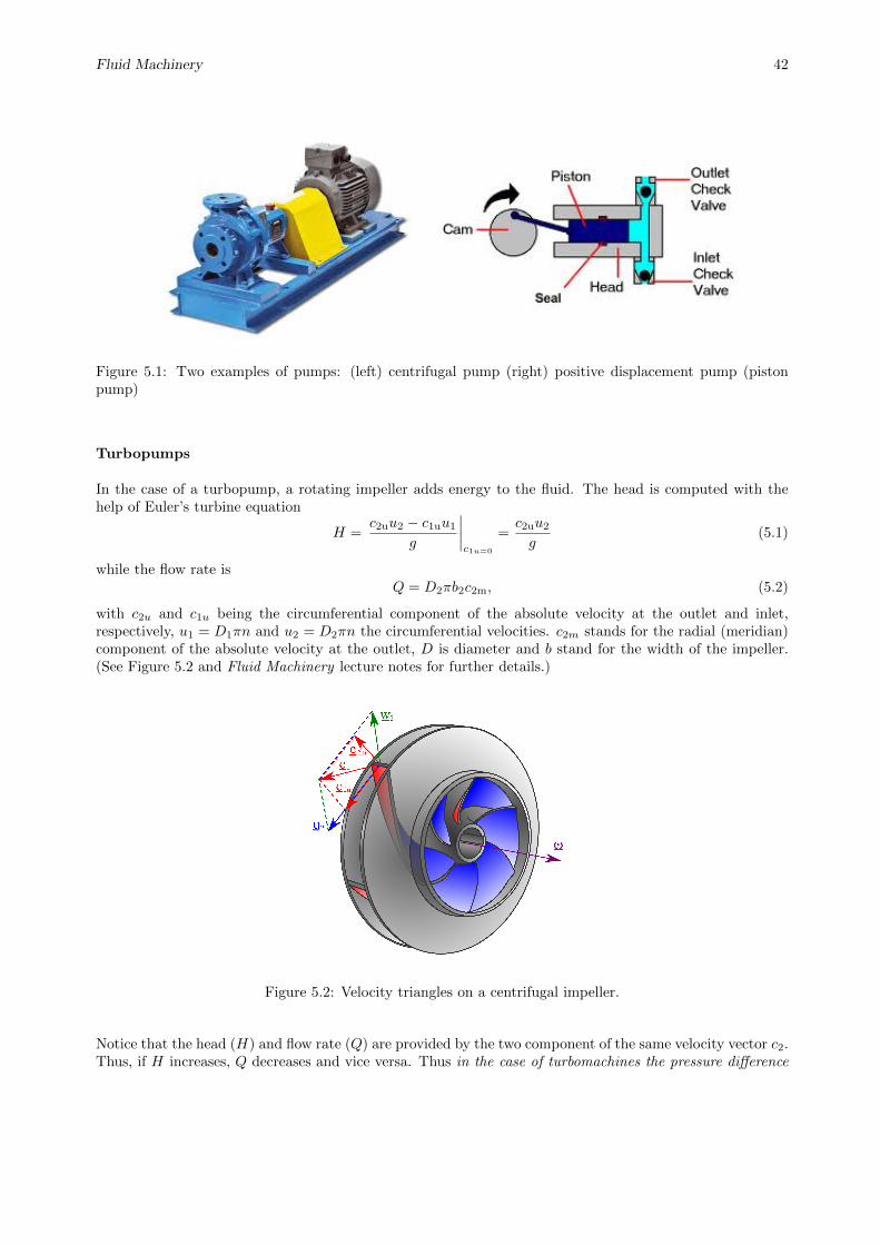
Figure 5.1: Two examples of pumps: (left) centrifugal pump (right) positive displacement pump (pistonpump)

Turbopumps

In the case of a turbopump, a rotating impeller adds energy to the fluid. The head is computed with thehelp of Euler’s turbine equation

H =c2uu2 − c1uu1

g

∣∣∣∣c1u=0

=c2uu2

g(5.1)

while the flow rate isQ = D2πb2c2m, (5.2)

with c2u and c1u being the circumferential component of the absolute velocity at the outlet and inlet,respectively, u1 = D1πn and u2 = D2πn the circumferential velocities. c2m stands for the radial (meridian)component of the absolute velocity at the outlet, D is diameter and b stand for the width of the impeller.(See Figure 5.2 and Fluid Machinery lecture notes for further details.)

Figure 5.2: Velocity triangles on a centrifugal impeller.

Notice that the head (H) and flow rate (Q) are provided by the two component of the same velocity vector c2.Thus, if H increases, Q decreases and vice versa. Thus in the case of turbomachines the pressure difference

Fluid Machinery 43

and the flow rate are directly connected and not independent. This dependency is described by the pump’sperformance curve, see Figure 5.3.

H, η

Q

design point

H(Q)

η(Q)ηmax.

Qopt.

Hopt.

Figure 5.3: Turbopump performance curves

An important quantity describing the shape of the impeller of a turbopump is the specific speed nq, definedas

nq = nQ

1/2opt.

H3/4opt.

[rpm][m3/s]1/2

[m]3/4. (5.3)

The dimension (unit) of nq is not emphasised and mostly omitted. The concept of specific speed can be usedto determine the pump type (i.e. radial/mixed/axial) which is capable of performing a pumping problemefficiently.

Capacity

Pow

er, h

ead,

effi

cien

cy

Pow

er, h

ead,

effi

cien

cy

Pow

er, h

ead,

effi

cien

cy

Capacity Capacity

40 60 80 100 150 200 30020

nq

Radial-vanes Francis-vanes Mixed-flow Axial-flow

Figure 5.4: Turbopump performance curves

Example 1. We have to pump clean water to an upper reservoir at 60 m height. The nominal power ofthe driving electric motor is 5 kW, its revolution number is 3000 rpm. The flow rate is (assuming 100%efficiency)

Pmotor = ∆p ·Q→ Q =Pmotor

∆p=Pmotor

ρgH= 8.49× 10−3 m3/s = 509 l/min (5.4)

Fluid Machinery 44

Hence the specific speed is

nq = nQ

1/2opt.

H3/4opt.

= 3000

(8.49× 10−3

)1/2(60)

3/4∼= 12.8, (5.5)

which means that a centrifugal turbopump is suitable for this problem.

Example 2. Now consider the hydraulic cylinder depicted in Figure 5.5. The required pressure differenceis now ∆p = 200bar = 2× 107Pa, the power and the revolution number of the driving motor is the same asbefore (5kW, 3000rpm).

m

p

Figure 5.5: Simple sketch of a hydraulic cylinder

First, find the flow rate of the pump (again, assume 100% efficiency):

Q =Pmotor

ρgH=

5000

9810 · 2000= 2.55× 10−4 m3/s = 15.3 liter/min, (5.6)

which gives

nq = nQ

1/2opt.

H3/4opt.

= 3000

(2.55× 10−4

)1/2(2000)

3/4= 0.16. (5.7)

Comparing this value with Figure 5.4 we see that this value is ’off’ the chart. Such a small nq valuewould require an extremely large-diameter impeller, which is very thin. Besides the problems with thehigh centrifugal stresses, from the fluid mechanical point of view, such a thin impeller introduces extremelylarge fluid friction resulting in poor efficiency. Thus we conclude that pumping problems resulting inhigh pressure difference and low flow rates (i.e. nq < say,10) cannot be efficiently solved bycentrifugal pumps.

Positive displacement pumps

Positive displacement pumps (PDPs) are typically used in high-pressure (above ∆p > 10bar, up to 1000-2000bars) technology, with relatively low flow rate. These machines have an expanding cavity on the suction sideand a decreasing cavity on the discharge side. Liquid flows into the pumps as the cavity on the suction sideexpands and the liquid flows out of the discharge as the cavity collapses. The volume is constant given eachcycle of operation.

The positive displacement pumps can be divided in two main classes (see Figures XXX)

� reciprocating

– piston pumps

– plunger pumps

– diaphragm pumps

– axial/radial piston pumps

Fluid Machinery 45

� rotary

– gear pumps

– lobe pumps

– vane pumps

– progressive cavity pumps

– peripheral pumps

– screw pumps

Figure 5.6: Some reciprocating pumps

Figure 5.7: Some rotary pumps

PDPs, unlike a centrifugal pumps, will produce the same flow at a given motor speed (rpm) no matter thedischarge pressure, hence PDPs are constant flow machines. A PDP must not be operated against a closedvalve on the discharge (pressure) side of the pump because it has no shut-off head like centrifugal pumps:

Fluid Machinery 46

a PDP operating against a closed discharge valve will continue to produce flow until the pressure in thedischarge line are increased until the line bursts or the pump is severely damaged - or both.

A relief or safety valve on the discharge side of the PDP is therefore absolute necessary. The relief valve canbe internal or external. The pump manufacturer has normally the option to supply internal relief or safetyvalves. The internal valve should in general only be used as a safety precaution, an external relief valveinstalled in the discharge line with a return line back to the suction line or supply tank is recommended.

Several types of PDPs can be used as motors: if fluid is driven through them (e.g. gear pump), the shaftrotates and the same machine can be used as a motor.

Fluid Machinery 47

5.1.2 Basic characteristics of positive displacement machines

The pump displacement Vg is the volume of the liquid delivered by the pump per one revolution, assum-ing no leakage (zero pressure difference between the suction and pressure side) and neglecting the fluidcompressibility. The ideal – theoretical – flow rate is

Qth = nVg (5.8)

where Qth is theoretical flow rate (liter/min), n is the revolution number of the pump shaft (rpm) and Vgstands for the pump displacement, (cm3).

In the case of pumps, the actual outflow is less than the theoretical flow rate, due to the leakages insidethe pump. These losses are taken into by the volumetric efficiency ηvol: Q = ηvolQth = ηvol nVg. Othertypes of losses (sealing, bearing, fluid internal and wall friction) are all concentrated into the so-calledhydromechanical efficiency ηhm, which connects the input and output power: Pinηhm = Pout. For pumps,Pin = Mω and Pout = Q∆p. We have:

ηhmM 2πn︸︷︷︸ω︸ ︷︷ ︸

Pin

= nVgηvol︸ ︷︷ ︸Q

∆p

︸ ︷︷ ︸Pout

→ ∆ppump =2πM

Vg

ηhmηvol

(5.9)

In the case of motors, the input power is hydraulic power (Pin = Q∆p) and the output is rotating mechanicalpower Pout = Mω. Due to the internal leakage, one has to ’push’ more fluid into the pump to experiencethe same revolution number, hence Q = Qth/ηvol > Qth. We have:

ηhmnVgηvol︸︷︷︸Q

∆p

︸ ︷︷ ︸Pin

= M 2πn︸︷︷︸ω︸ ︷︷ ︸

Pout

→ ∆pmotor =2πM

Vg

ηvolηhm

(5.10)

H (~Δp)

Q

n1

motor @ n1

theoretical @ n1

motor @ n2

pump @ n2 pump @ n1

n2<n1

Figure 5.8: Pump and motor performance curves for two different revolution mubers.

We conclude that for both pumps and motors,

Q ∝ n, Vg and ∆p ∝M,1

Vg.

(5.11)

Fluid Machinery 48

Which means that the pressure and the flow rate are independent for a given machine. The same behaviourcan be observed on the performances curve of these machines, see Figure 5.8. The theoetical performancelines are vertical for a given revolution speed, meaning that the theoretical flow rate does not change whenvarying the pressure.

However, the leakage flow rate through the small internal gaps of the pumps (motors) slighty change thstheoretical behaviour. In the case of pumps, a portion of the flow rate flows back from the pressure sideto the suction side through these gaps, hence reducing the outflow of the pump. The higher the pressuredifference is, the higher the leakage flow rate is, hence the pump performance curves tend to ‘bend to theleft’ from the vertical, theoretical line. In the case of motors, where the fluid drives the shaft, we need largerflow rates to reach the desired revolution number, hence the real curves ‘bend to the right’.

Fluid Machinery 49

5.2 Reciprocating Pumps

Piston/plunger pumps comprise of a cylinder with a reciprocating piston/plunger in it. In the head of thecylinder the suction and discharge valves are mounted. In the suction stroke the plunger retracts and thesuction valves opens causing suction of fluid into the cylinder. In the forward stroke the plunger push theliquid out the discharge valve.

With only one cylinder the fluid flow varies between maximum flow when the plunger moves through themiddle positions, and zero flow when the plunger is in the end positions. A lot of energy is wasted whenthe fluid is accelerated in the piping system. Vibration and ”water hammers” may be a serious problem. Ingeneral the problems are compensated by using two or more cylinders not working in phase with each other.

Several cylinders can be mounted to the same shaft: pumps with 1 cylinder are called simplex pumps, duplexpumps have two cylinders (with π phase shift) while triplex pumps have three pumps with 2π/3 = 120degrees phase shift. Pumps with even more pistons (5,7,9) are also common. Pumps with both sides of thepiston acting (deing in contact with the liquied) are called double-acting pumps.

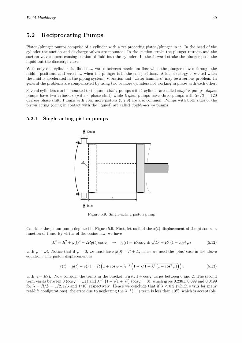
5.2.1 Single-acting piston pumps

Inlet

Outlet

A

s

Figure 5.9: Single-acting piston pump

Consider the piston pump depicted in Figure 5.9. First, let us find the x(t) displacement of the piston as afunction of time. By virtue of the cosine law, we have

L2 = R2 + y(t)2 − 2Ry(t) cosϕ → y(t) = R cosϕ±√L2 +R2 (1− cos2 ϕ) (5.12)

with ϕ = ωt. Notice that if ϕ = 0, we must have y(0) = R + L, hence we need the ’plus’ case in the aboveequation. The piston displacement is

x(t) = y(t)− y(π) = R(

1 + cosϕ− λ−1(

1−√

1 + λ2 (1− cos2 ϕ)))

, (5.13)

with λ = R/L. Now consider the terms in the bracket. First, 1 + cosϕ varies between 0 and 2. The secondterm varies between 0 (cosϕ = ±1) and λ−1

(1−√

1 + λ2)

(cosϕ = 0), which gives 0.2361, 0.099 and 0.0499for λ = R/L = 1/2, 1/5 and 1/10, respectively. Hence we conclude that if λ < 0.2 (which s trus for manyreal-life configurations), the error due to neglecting the λ−1(. . . ) term is less than 10%, which is acceptable.

Fluid Machinery 50

Hence we approximate the piston displacement as

x(t) ≈ R (1 + cos (ωt)) , v(t) ≈ −Rω sin (ωt) and a(t) ≈ −Rω2 cos (ωt) . (5.14)

As flow rate is Q = Av and the stroke is s = 2R, the instantaneous pressure side flow rate is (see also Figure5.10)

Q(t) =

{A s

2ω cos(ωt) if π < ϕ = ωt < 2π

0 if 0 < ϕ = ωt < π(5.15)

The mean flow rate is computed by finding the volume of the fluid pushed to the pressure side in one period,divided by the length of the period:

Qmean = Asn, (5.16)

that is, we have Vg = As, see (5.8). The maximum flow rate is (see (5.15))

Qmax = As

2ω = πAsn = πQmean. (5.17)

x(t)

Q(t)

t

tT 2T

T 2T

s/2

Aωs/2

-s/2

-Aωs/2

V

Figure 5.10: Piston displacement (upper panel) and flow rate (∝ velocity) curves of a single-acting pistonpump.

Notice that this means that these pumps induce an extremely unsteady flow rate in the pipeline system,that varies from Qmin = 0 flow rate up to Qmax = πQmean with a frequency of n (driving motor revolutionnumber). There are two ways of reducing this pulsation: (a) by using multiple pistons or (b) adding apulsation damper.

Fluid Machinery 51

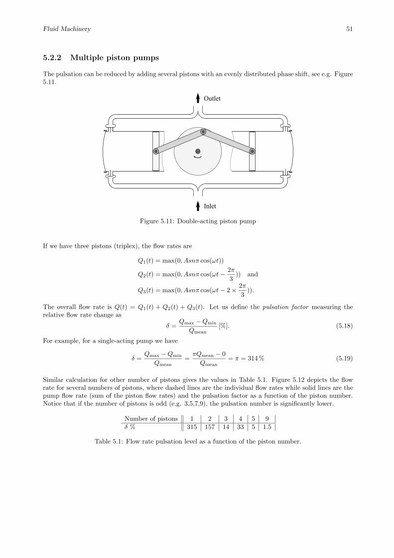
5.2.2 Multiple piston pumps

The pulsation can be reduced by adding several pistons with an evenly distributed phase shift, see e.g. Figure5.11.

Inlet

Outlet

Figure 5.11: Double-acting piston pump

If we have three pistons (triplex), the flow rates are

Q1(t) = max(0, Asnπ cos(ωt))

Q2(t) = max(0, Asnπ cos(ωt− 2π

3)) and

Q3(t) = max(0, Asnπ cos(ωt− 2× 2π

3)).

The overall flow rate is Q(t) = Q1(t) + Q2(t) + Q3(t). Let us define the pulsation factor measuring therelative flow rate change as

δ =Qmax −Qmin

Qmean[%]. (5.18)

For example, for a single-acting pump we have

δ =Qmax −Qmin

Qmean=πQmean − 0

Qmean= π = 314 % (5.19)

Similar calculation for other number of pistons gives the values in Table 5.1. Figure 5.12 depicts the flowrate for several numbers of pistons, where dashed lines are the individual flow rates while solid lines are thepump flow rate (sum of the piston flow rates) and the pulsation factor as a function of the piston number.Notice that if the number of pistons is odd (e.g. 3,5,7,9), the pulsation number is significantly lower.

Number of pistons 1 2 3 4 5 9δ % 315 157 14 33 5 1.5

Table 5.1: Flow rate pulsation level as a function of the piston number.

Fluid Machinery 52

0 T/2 T 3T/2 2T0

0.5

1

N=1

0 2 4 6 8 10 1210

0

101

102

103

Number of pistons

puls

atio

n fa

ctor

[%]

0 T/2 T 3T/2 2T0

0.5

1

N=2

0 T/2 T 3T/2 2T0

0.5

1

N=3

0 T/2 T 3T/2 2T0

1

N=4

0 T/2 T 3T/2 2T0

1

N=5

0 T/2 T 3T/2 2T0

1

2

N=6

0 T/2 T 3T/2 2T012

N=7

0 T/2 T 3T/2 2T0

2

N=8

Figure 5.12: Pulsation factor as a function of the piston number.

Fluid Machinery 53

5.2.3 Axial piston pumps

An axial piston pump is a positive displacement pump that has a number of pistons in a circular array withina cylinder block. It can be used as a stand-alone pump, a hydraulic motor or an automotive air conditioningcompressor. Axial piston pumps are used to power the hydraulic systems of jet aircrafts, being gear-drivenoff of the turbine engine’s main shaft. The system used on the F-14 used a 9-piston pump that produced astandard system operating pressure of 3000 psi and a maximum flow of 84 gallons per minute. Advantages:

� high efficiency

� high pressure (up to 1,000 bar)

� low flow and pressure ripple (due to the small dead volume in the workspace of the pumping piston)

� low noise level

� high reliability

Axial piston units are available in the form of pumps and motors in bent axis design or swashplate designfor medium- and high-pressure ranges. They are the main components in the hydrostatic transmission.Compact size and high power density, economy and reliability are characteristic advantages which speak forthe use of hydrostatic transmissions, together with the fact that they meet the demand for high speed andhigh torque, as well as optimum efficiency.

Figure 5.13: Axial piston pump

5.2.4 Radial piston pumps

In a radial piston pump the working pistons extend in a radial direction symmetrically around the driveshaft, in contrast to the axial piston pump. These kinds of piston pumps are characterized by the followingadvantages:

� high efficiency

� high pressure (up to 1,000 bar)

� low flow and pressure ripple (due to the small dead volume in the workspace of the pumping piston)

� low noise level

� very high load at lowest speed due to the hydrostatically balanced parts possible

Fluid Machinery 54

� no axial internal forces at the drive shaft bearing

� high reliability

A disadvantage are the bigger radial dimensions in comparison to the axial piston pump, but it could becompensated with the shorter construction in axial direction.

Due to the hydrostatically balanced parts it is possible to use the pump with various hydraulic fluids likemineral oil, biodegradable oil, HFA (oil in water), HFC (water-glycol), HFD (synthetic ester) or cuttingemulsion. That implies the following main applications for a radial piston pump: machine tools (e.g.,displace of cutting emulsion, supply for hydraulic equipment like cylinders)

� high pressure units (HPU) (e.g., for overload protection of presses)

� test rigs

� automotive sector (e.g., automatic transmission, hydraulic suspension control in upper-class cars)

� plastic- and powder injection moulding

� wind energy

Figure 5.14: Radial piston pump

5.2.5 Diaphragm pumps

A diaphragm pump (also known as a membrane pump) is a positive displacement pump that uses a combi-nation of the reciprocating action of a rubber, thermoplastic or teflon diaphragm and suitable valves eitherside of the diaphragm (check valve, butterfly valves, flap valves, or any other form of shut-off valves) topump a fluid. The advantages of these pumps are:

� They provide leakage-free sealing, which can be important when pumping highly aggressive or toxicfluids.

� They have good suction lift characteristics, some are low pressure pumps with low flow rates; othersare capable of higher flow rates, dependent on the effective working diameter of the diaphragm and itsstroke length.

� They can handle sludges and slurries with a relatively high amount of grit and solid content.

� Suitable for discharge pressure up to 1200 bar

Fluid Machinery 55

� They have good dry running characteristics.

� Good efficiency (can be up to 97%)

� Can handle highly viscous liquids.

However, as they are single (or sometimes double-acting) piston pumps, these pumps cause a pulsating flowthat may cause water hammer, which can be minimised by using a pulsation dampener.

Figure 5.15: Diaphragm pump

Fluid Machinery 56

5.3 Rotary pumps

5.3.1 Gear pumps

This is the simplest of rotary positive displacement pumps consisting of two meshed gears rotating in aclosely fitted casing. Fluid is pumped around the outer periphery by being trapped in the tooth spaces. Itdoes not travel back on the meshed part, since the teeth mesh closely in the centre. It is widely used on carengine oil pumps, and also in various hydraulic power packs.

There are two main variations; external gear pumps which use two external spur gears, and internal gearpumps which use an external and an internal spur gear. Some gear pumps are designed to function as eithera motor or a pump.

Figure 5.16: (left) external gear pump (right) internal gear pump

External gear pumps

Advantages:

� High speed

� High pressure

� Relatively quiet operation

Disadvantages:

� Four bushings in liquid area

� No solids allowed

� Fixed end clearances

Common external gear pump applications include, but are not limited to:

� Various fuel oils and lube oils

� Chemical additive and polymer metering

� Chemical mixing and blending (double pump)

� Industrial and mobile hydraulic applications (log splitters, lifts, etc.)

� Acids and caustic (stainless steel or composite construction)

Fluid Machinery 57

Internal gear pumps

Advantages:

� Only two moving parts

� Only one stuffing box

� Non-pulsating discharge

� Excellent for high-viscosity liquids

� Operates well in either directions

� Low NPSH required

� Single adjustable end clearance

� Easy to maintain

Disadvantages:

� Usually requires moderate speeds

� Medium pressure limitations

� One bearing runs in the product pumped

Common internal gear pump applications include, but are not limited to:

� All varieties of fuel oil and lube oil

� Resins and polymers

� Alcohols and solvents

� Asphalt, bitumen, and tar

� Food products such as corn syrup, chocolate, and peanut butter

� Paint, inks, and pigments

� Soaps and surfactants

� Glycol

5.3.2 Screw pump

Screw pumps feature two or three screws with opposing thread, that is, one screw turns clockwise, and theother counterclockwise. The screws are each mounted on shafts that run parallel to each other; the shaftsalso have gears on them that mesh with each other in order to turn the shafts together and keep everythingin place. The turning of the screws, and consequently the shafts to which they are mounted, draws thefluid through the pump. As with other forms of rotary pumps, the clearance between moving parts and thepump’s casing is minimal.

Advantages:

� Practically pulsation-free flow

� low fluid velocities → not sensitive for e.g. sand content

Disadvantages:

� Expensive

Fluid Machinery 58

Figure 5.17: (left) simple screw pump (right) double-screw pump used for pumping crude oil

5.3.3 Vane pump

Advantages:

� Handles thin liquids at relatively higher pressures

� Sometimes preferred for solvents, LPG

� Can run dry for short periods

� Develops good vacuum

Disadvantages:

� Not suitable for high pressures

� Not suitable for high viscosity

� Not good with abrasives

Applications:

� Aerosol and Propellants

� Aviation Service - Fuel Transfer, Deicing

� Auto Industry - Fuels, Lubes, Refrigeration Coolants

� Bulk Transfer of LPG and NH3

� LPG Cylinder Filling

� Alcohols

� Refrigeration - Freons, Ammonia

Fluid Machinery 59

Figure 5.18: Vane pump

5.3.4 Progressing cavity pump (eccentric screw pump)

Widely used for pumping difficult materials such as sewage sludge contaminated with large particles, thispump consists of a helical shaped rotor, about ten times as long as its width. This can be visualized as acentral core of diameter x, with typically a curved spiral wound around of thickness half x, although of coursein reality it is made from one casting. This shaft fits inside a heavy duty rubber sleeve, of wall thicknesstypically x also. As the shaft rotates, fluid is gradually forced up the rubber sleeve. Such pumps can developvery high pressure at quite low volumes.

Figure 5.19: Progressive cavity pump.

5.3.5 Peristaltic pump

A peristaltic pump is a type of positive displacement pump used for pumping a variety of fluids. The fluidis contained within a flexible tube fitted inside a circular pump casing (though linear peristaltic pumps havebeen made). A rotor with a number of ”rollers”, ”shoes” or ”wipers” attached to the external circumferencecompresses the flexible tube. As the rotor turns, the part of the tube under compression closes (or ”occludes”)thus forcing the fluid to be pumped to move through the tube. Additionally, as the tube opens to its naturalstate after the passing of the cam (”restitution”) fluid flow is induced to the pump. This process is calledperistalsis and is used in many biological systems such as the gastrointestinal tract.

Fluid Machinery 60

Advantages

� No contamination. Because the only part of the pump in contact with the fluid being pumped is theinterior of the tube, it is easy to sterilize and clean the inside surfaces of the pump.

� Low maintenance needs. Their lack of valves, seals and glands makes them comparatively inexpensiveto maintain.

� They are able to handle slurries, viscous, shear-sensitive and aggressive fluids.

� Pump design prevents backflow and syphoning without valves.[5]

Disadvantages

� The flexible tubing will tend to degrade with time and require periodic replacement.

� The flow is pulsed, particularly at low rotational speeds. Therefore, these pumps are less suitablewhere a smooth consistent flow is required. An alternative type of positive displacement pump shouldthen be considered.

Figure 5.20: Peristaltic pump

Fluid Machinery 61

5.3.6 Pulsation dampener

A pulsation dampener is an accumulator with a set pre-charge that absorbs system shocks while minimizingpulsations, pipe vibration, water hammering and pressure fluctuations. By minimizing pulsation in thesystem components like regulators, solenoids, sensors, etc., pumps will see decreased wear and have longerlife. Pulsation dampeners are tied directly onto the discharge manifold or plumbed immediately downstreamof the pump.

Figure 5.21: Pulsation dampener.

The sizing of the dampener goes as follows. The instantaneous and mean flow rate for a single piston pumpis

Q(t) = Qmax sin(ωt) and Qmean =Qmaxπ

, where Qmax = πADsn. (5.20)

The pump flow rate is Qp(t) =∑Ni=1Qi(t), where Qi is the flow rate of the ith piston, i.e. (5.20) shifted

with an angle of φi = (i − 1) 2π/N , N being the number of pistons. The average flow rate of the pump isQp,mean = N Qmean.

The flow rate entering the damper is

Qd(t) = Qp(t)−Qp,mean, (5.21)

while the volume of fluid entering (or leaving) the damper up to time t is

Vd(t) =

∫Qd(t)dt. (5.22)

In the case of a single piston, we have

Qd(t) =

{Qmax

(sin(ωt)− 1

π

)if 0 ≤ t ≤ T

2

−Qmax/π if T2 ≤ t ≤ T

and (5.23)

Vd(t) =

{Qmax

(− 1ω (cos(ωt)− 1)− t

π

)if 0 ≤ t ≤ T

2

−tQmax/π if T2 ≤ t ≤ T.

(5.24)

The above expression for Vd also ensures that Vd(0) = 0. Maximum and minimum volume occurs at Qp = 0,

Fluid Machinery 62

i.e.

ωtmin = arcsin1

π→ tmin =

0.3239

2πT = 0.0516T. (5.25)

ωtmax = π − arcsin1

π→ tmax =

π − 0.3239

2πT = 0.4484T. (5.26)

The corresponding volumes are

Vmin = −0.0081QmaxT = −0.0081π︸ ︷︷ ︸−0.0256

QmeanT︸ ︷︷ ︸Vstroke

and Vmin = 0.1673QmaxT = 0.5256Vstroke, (5.27)

hence the total volume variation on the damper is

∆V = Vmax − Vmin = 0.55Vstroke (5.28)

A similar calculation for a double-acting piston gives

tmin = 0.1098T, tmax = 0.3902T and ∆V = Vmax − Vmin = 0.2105Vstroke (5.29)

For pumps with 3 or 4 pistons, the analytical derivation is cumbersome, instead, one can simply plot thegraphs and evaluate the results numerically giving ∆V = 0.009Vstroke for triplex and ∆V = 0.044Vstroke forfour-cylinder pumps, see Figure 5.22. The volume change is given in the percentage of the stroke:

∆V = νVstroke, with

{N = 1 2 3 4ν = 0.55 0.21 0.044 0.009

(5.30)

0 T/2 T−20

0

20

40

60N=1, dV=55.1%

% o

f pis

ton

stro

ke

0 T/2 T−20

0

20

40

60N=2, dV=21.2%

% o

f pis

ton

stro

ke

0 T/2 T−20

0

20

40

60N=3, dV=0.9%

% o

f pis

ton

stro

ke

0 T/2 T−20

0

20

40

60N=4, dV=4.3%

% o

f pis

ton

stro

ke

Figure 5.22: Volume change in the pressure dampener for different number of pistons.

Fluid Machinery 63

Now let us find the pressure pulsation of the gas due to the fluid volume change ∆V . We start off by definingthe pre-charge pressure ppc (e.g. 80% of system pressure), at which the gas volume is V0 (i.e. the nominalvolume of the damper) and the required level of damping δ = (pmax − pmin)/psys. The corresponding gasvolumes will be Vmax (corresponding to pmin) and Vmin (corresponding to pmax). At system pressure, thethe gas volume is Vsys. We also have V gmax = V gmin + ∆V .

Notice that if the process is isotherm (which is usually true in real-life cases), we have)

δ =pmax − pmin

psys=

∆p

psys≈ ∆V

Vsys(5.31)

We also have

pmin = ppcV0

Vmax, psys = ppc

V0

Vsysand pmax = ppc

V0

Vmin, (5.32)

and the pressure pulsation level is

δ =∆V

Vsys=νVstrokeV0

ppcpsys

(5.33)

hence the required dampener volume is

V0 =νVstrokeppcpsys

δ

(5.34)

Example. We have a duplex pump (N = 2, ν = 0.2105) with s = 60mm stroke and D = 63mm diameter.

� The stroke volume is Vstroke = D2π4 s = 0.187 liter

� The precharge pressure is set to 80% of system pressure: ppc/psys = 0.8

� The required level of damping is δ = 5%.

� The nominal dampener volume is V0 = 0.2105×0.1870.8×0.05 = 0.984 ≈ 1 liter.

Fluid Machinery 64

5.4 Pressure relief valves (PRV)

As we have seen, the flow rate of a PDP is hardly affected by the system pressure, hence even if the flow rateneed of the system is zero, the pump will convey the flow rate into the system. In such cases, the systempressure quickly rises and, if not vented, some component will break leading to a failure in the system. Toprevent such problems, pressure relief valve (PRV) must are mounted as close to the pump as possible.

These devices open above a set pressure allowing controlled backflow to the the tank. If the system pressureis below the st pressure, the PRV remains closed and does not affect the system behaviour. There are twomain types:

Direct spring loaded: Usually used for low flow rate.

Pilot operated: High flow rate.

5.4.1 Direct spring loaded hydraulic PRV

Direct spring loaded pressure relief valves (DSLPRV) are simple and robust. The spool is balanced by aspring (upper side) and the pressure force (lower side). Note that the flow-through area varies with the valvelift (see Figures 5.23 and 5.24).

Q to system

A

spool

spring

p

Figure 5.23: Direct spring loaded hydraulic PRV

The force balance of the spool reads

s (x+ x0) = A∆p. (5.35)

The set pressure, at which the valve opens is given by pset = sx0

A . In general, the flow rate is Q =

Fluid Machinery 65

Q

ØD

xxmax

Figure 5.24: Detail of a direct spring loaded hydraulic PRV

CdAft√

2∆p/ρ. However, it should be noted that the flow-through area varies with the valve lift:

Q(∆p) =

0 for x < 0

CdAft(x)√

2ρ∆p = CdDπ

(A∆p

s− x0

)︸ ︷︷ ︸

x

√2ρ∆p for 0 < x < xmax

CdDπxmax

√2ρ∆p for x > xmax

(5.36)

Note that in the middle range, we have

Q(∆p) = CdDπA

s

√2

ρ

(∆p− x0s

A

)√∆p ∝ (∆p− pset)

√∆p, (5.37)

that is, it is zero if ∆p = 0 and ∆p = pset. Moreover, for 0 ≤ ∆p ≤ pset this function is negative, for∆p > pset, the flow rate is proportional to ∆p3/2. The actual plot is shown in Figure 5.26.

Q

ΔpΔpset

xmax

p

p

( p-pset)

Figure 5.25: Q(∆p) curve of a direct spring loaded hydraulic PRV

∆p in normal operation: ∆p ·√

∆p = ∆p3/2 → it is between ∆p . . .∆p3/2 . . .∆p2 The usual way of plottingthe characteristic curve is inverse (also in catalogue): Note: ∆pstatic ≈ (0.01 . . . 0.1)∆pset.

Dynamic error

When it opens quickly. Note: ∆pdyn can be 2 . . . 3 times bigger than ∆pset.

Fluid Machinery 66

Q

Δp

Δpset

Qnominal

normal operation overload

Δpstatic error

Figure 5.26: Inverse Q(∆p) curve of a direct spring loaded hydraulic PRV

t

Δp

dynamic error

Δpset

Figure 5.27: Dynamic error of a direct spring loaded hydraulic PRV

Sizing of a pressure relief valve

Qpump,max < QPRV,max (5.38)

Examples

Hydraulic aggregate Pump and PRV.

In gas systems Natural gas industry.

Fluid Machinery 67

Figure 5.28: Standard symbol of PRV

Qpump

Qsystem

Qvalve

Figure 5.29: Hydraulic aggregate

Q

Δp

Qpump

Figure 5.30: 19 caption

Fluid Machinery 68

Q

Δp

BadGood

Figure 5.31: 20 caption

from reservoir

to system

Figure 5.32: PRV used in natural gas industry

Fluid Machinery 69

5.4.2 Pilot operated pressure relief valve

As Qnominal increases, the static error also increases. In this case we can use pilot operated PRV.

Q

Δp

Δpstat. error

Figure 5.33: Static error of a direct spring loaded PRV

Q = CdDπ

(A∆p

s− x0

)√2

ρ∆p (5.39)

Let Qnominal be given: Q at ∆pmax

∆pset be given: ∆pset = sx0

A

If higher flow rate is needed: increase D.

sx0

A=

sx0

D2π4

= ∆pset (5.40)

Increase s (stiffer spring)) or x0 (higher precompression) to keep ∆pset as constant value.

However the slope of the curve in the normal operation:

d

d∆pQ =

d

d∆p

(CdDπ

(D2π

4s

)√2

ρ∆p3/2

)∼ D3

s

3

2

√∆p (5.41)

and s ∼ D2.

1st choise Let s ∼ D2. ∆pset = sx0D2π

4

remains constant. Slope ∼ static error ∼ D.

2nd choise s is constant x0 ∼ D2 → slope ∼ D3. Too high static error! Solution: pilot operated PRV.

Operating progress of the valve

Pressure drops because of the fixed orifice → the spool moves upwards → it opens the main opening.

Important details

– Right location of the soft and hard springs

– Fixed orifice

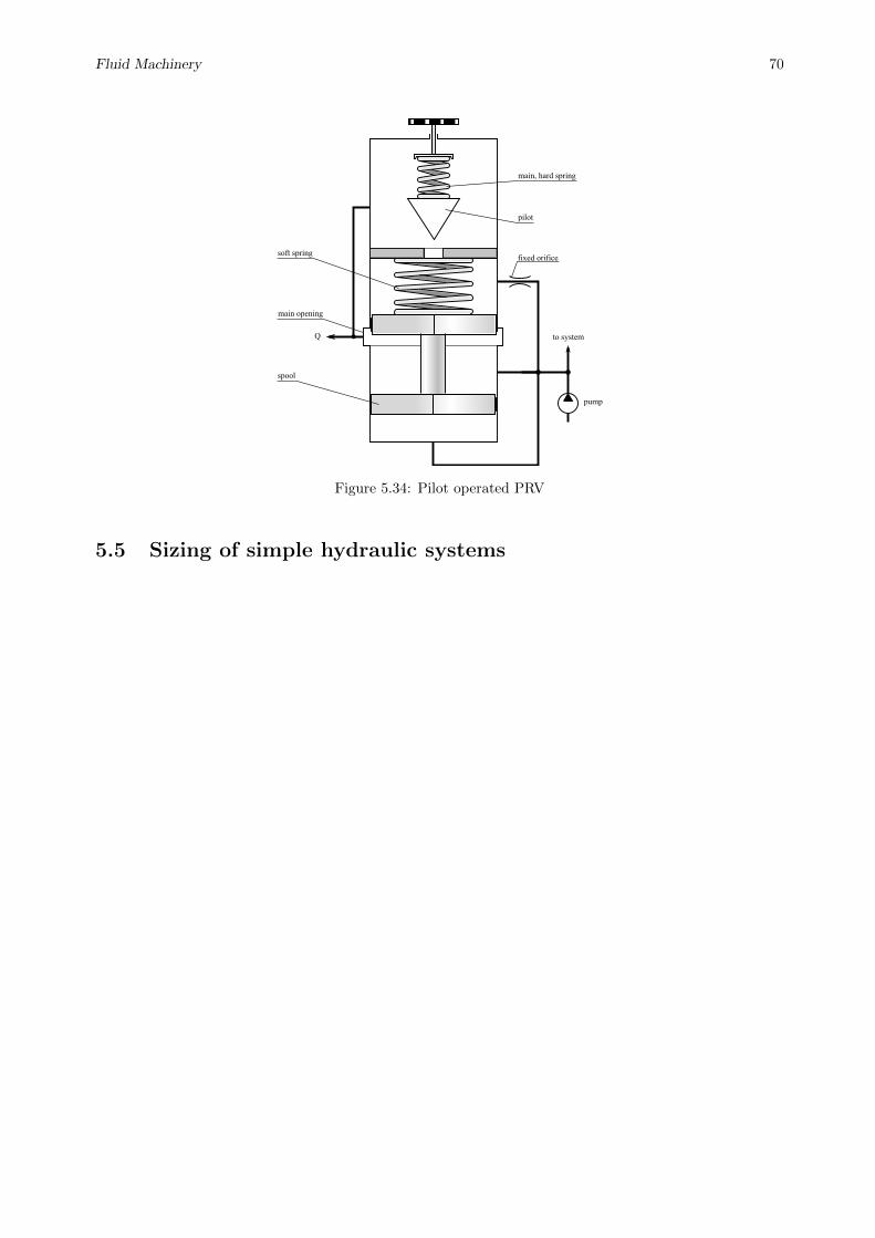
Fluid Machinery 70

Q to system

pilot

fixed orifice

main, hard spring

soft spring

main opening

spool

pump

Figure 5.34: Pilot operated PRV

5.5 Sizing of simple hydraulic systems

Fluid Machinery 71

5.5.1 System with motor

Figure 5.35: Hydraulic aggregate with motor

User data: Mmotor, nmotor

Sizing: Vg,pump, pset, Vg,motor, control

Example for a system with motor

Mmotor = 100 Nm, nmotor = 1500 rpm

MotorQ∆pηhm = M2πn (5.42)

∆p ∼M and Q ∼ n → Vg

From catalogue: ∆p = 280 bar → size: 23 → Mmotor = 105 Nm and Vg = 23.5 cm3

Qmotor = Vgnmotor = 23.5× 10−3 l/min× 1.5× 103 1/min = 35.25 l/min (5.43)

Output of the sizing: ∆p, Q. In this calculation η ∼= 1.

5.5.2 System with cylinder

Figure 5.36: Hydraulic aggregate with cylinder

User data: F , vSizing: Vg,pump, pset,

Dd , control

Piston control valve From catalogue: Vg,pump, Vg,motor,Dd

Fluid Machinery 72

Figure 5.37: Symbol of the piston control valve

from pump to system

Figure 5.38: Piston control valve with cylinder

Example for a system with cylinder

Mmotor = 100 Nm, nmotor = 1500 rpmnVg∆p = M2πn (5.44)

∆p =M2πn

nVg=

2πM

Vg=

2π100

Vg=

2π100

28.5× 10−6= 220 bar (5.45)

Q = Vgnmotor = 28.5× 1.5 = 42.75 l/min (5.46)

Pick size 28. The aggregate should provide this flow rate at the ∆p pressure.

Pump Driving motor speed: npump = 3000 rpm

Qpump = npumpVg,pump → Vg,pump =Qpump

npump=

28.5 l/min

3000 rpm= 14.25 cm3 (5.47)

Pick Vg,pump = 16 cm3. With the new value:

Qpump = npumpVg,pump = 3000 rpm× 16 cm3 = 48 l/min (5.48)

Set pressure of the PRV 120 % of the highest expected system pressure.

pset := 1.2× 220 = 264 bar (5.49)

Qnom,PRV > 42.8 l/min (capacity of PRV).

5.5.3 Control techniques

– Throttle valve in parallel connection

– Throttle valve in series connection

Fluid Machinery 73

– Frequency converter

– Special pump: variable displacement motor, variable Vg

– Motor speeed (n) changing

Throttle valve in parallel connection

Qp Qv Qm

Figure 5.39: System with throttle valve in parallel connection

∆p is the same. PRV is closed.

Throttle valve in series connection

Δpv

Δpm

Figure 5.40: System with throttle valve in series connection

Q is the same. PRV is open.

5.6 Problems

Problem 5.6.41

Calculate the hydraulic power of the double-acting piston pump, which delivers water from an open-surfacetank into a closed one with 500[kPa] gauge pressure (i.e. relative pressure) located 50[m] above the suctiontank. Diameter of the piston is D = 120[mm], the stroke is 150[mm] and the driving motor runs at 120[rpm].

Solution:

Qmean = 2×Apiston × s× n = 2× 0.122π4 × 0.15× 120

60 = 6.78× 10−3[m3

s ]

∆p = ptank,abs. − p0 + ρgH = ptank,rel. + ρgH = 991[kPa]

Fluid Machinery 74

P = Q∆p = 6.72[kW ]

Problem 5.6.42

The characteristic curve of a gear pump is Q[dm3/min] = 11.93− 0.0043∆p[bar]. The volumetric efficiencyat 35bar pressure difference is 92%. Find the volume flow rate and the geometric volume! The shaft speed is80rev/min. How large is the driving torque if the pump efficiency is 85%? (Solution: Q = 11.78 dm3/min,Vg = 160 cm3, M = 96.5Nm)

Problem 5.6.43

The piston diameter of a hydraulic cylinder is 50mm. An 800kg load is lifted by the piston rod of 20mmdiameter with 12m/min velocity. How large must be the flow rate Q of the gear pump rotating withn = 960/min speed if its volumetric efficiency is 92%? Find the geometric volume of the pump and thepressure rise produced by it! Find the power P and the torque M of the driving motor! The pump efficiencyis 74%. Prepare a sketch of the gear pump showing the rotation direction of the shafts, intake and deliveryports! How large will be P ′, M , Q′ if the rotor speed is n′ = 1440/min? (Solution: Qg = 21.5 dm3/min,Vg = 22.4 cm3, ∆p = 47.6 bar, P = 2.12 kW , M = 21.1Nm, P1440 = 3.18 kW , Q1440 = 32.25 dm3/min,M1440 = 21.1Nm)

Problem 5.6.44

The piston diameter of a vertical hydraulic cylinder is supporting a mass of 700kg. It may not be loweredfaster than 64mm/s. The cylinder diameter is 50mm, the piston rod diameter is 28mm. The pump deliverycurve is Q[liter/min] = 8.6 − 0.0467∆p[bar]. The hydraulic oil of 970kg/m3 density leaves the cylinderthrough a throttle valve. The discharge coefficient of this valve is µ = 0.7. Find the valve area at themaximal opening! (Solution: Amax = 1.354mm2)

Chapter 6

Hydro- and wind power

6.1 Problems

Problem 6.1.45

The cross-section of a plant water channel is given. The measured average water depth is h = 2.9 m, thewidth of the channel is B = 25 m. The velocity of the water flow is measured at several locations of the cross-section using a cup-type anemometer. The calculated average velocity is v = 0.4 m/s. The height differencebetween the upstream and downstream water depth at the dam is hupstream − hdownstream = 4.5 m. Theefficiency of the turbine is ηturbine = 90 % the efficiency of the generator is ηgenerator = 96 %. The inputpower and useful power of the power plant are to be calculated. What is the value of the hydraulic radius?What type of turbine is suitable for this power plant?

Solution:

� A = hB = 72.5 m2

� Q = Av = 29 m3/s

� H = hupstream − hdownstream = 4.5 m

� P input = QρgH = 1.28 MW

� Puseful = ηturbineηgeneratorP input = 1.106 MW

� Rh = AreaPerimeter = Bh

2h+B= 2.35 m

Turbine type: Kaplan turbine.

Problem 6.1.46

The instantaneous efficiency of an existing wind turbine is to be calculated. The measured average windspeed at the level of the rotor is v1 = 12 m/s. The average speed of the air behind the rotor is v3 = 8 m/s.The diameter of the rotor is D2 = 55 m, the density of the air is ρair = 1.2 kg/m3. Find the calculatedefficiency related to the theoretical maximum of the efficiency?

Solution:

� ∆v = v1 − v3 = 4 m/s

75

Fluid Machinery 76

� A2 =D2

2π4 = 2376 m2

� P input = ρairA2v1v212 = 2.463 MW

� Puseful = ρairA2v31

(1− ∆v

2v1

)2∆vv1

= 1.140 MW

� η = CP =PusefulP input

= 0.463 < 1627 = 0.593

Problem 6.1.47

How large is the power of a wind turbine of 30m rotor diameter if the wind speed is 8m/s? The Betz limitof the power coefficient Cp is 0.593.