Fluid MachineryLecture notes

Mechanical Engineering Department College of Engineering

MINDANAO STATE UNIVERSITY

Contents

1 Some basic relationships of fluid mechanics and thermodynamics 3

1.1 Continuity equation . . . . . . . . . . . . . . . . . . . . . . . . . . . . . . . . . . . . . . . . . 3

1.2 Bernoulli’s equation . . . . . . . . . . . . . . . . . . . . . . . . . . . . . . . . . . . . . . . . . 4

1.3 Energy equation for compressible flow . . . . . . . . . . . . . . . . . . . . . . . . . . . . . . . 4

1.4 Thermodynamics . . . . . . . . . . . . . . . . . . . . . . . . . . . . . . . . . . . . . . . . . . . 5

1.4.1 Specific heat capacities . . . . . . . . . . . . . . . . . . . . . . . . . . . . . . . . . . . . 5

1.4.2 Some basic thermodynamic relationships . . . . . . . . . . . . . . . . . . . . . . . . . . 5

1.4.3 Input shaft work and useful work . . . . . . . . . . . . . . . . . . . . . . . . . . . . . . 6

1.4.4 Specific work for hydraulic machines . . . . . . . . . . . . . . . . . . . . . . . . . . . . 7

1.4.5 Efficiency . . . . . . . . . . . . . . . . . . . . . . . . . . . . . . . . . . . . . . . . . . . 7

1.5 Problems . . . . . . . . . . . . . . . . . . . . . . . . . . . . . . . . . . . . . . . . . . . . . . . 7

2 Incompressible turbomachinery 10

2.1 Euler’s turbine equation . . . . . . . . . . . . . . . . . . . . . . . . . . . . . . . . . . . . . . . 10

2.2 Velocity triangles and performance curves . . . . . . . . . . . . . . . . . . . . . . . . . . . . . 11

2.2.1 Radial (centrifugal) machines . . . . . . . . . . . . . . . . . . . . . . . . . . . . . . . . 12

2.2.2 Problems . . . . . . . . . . . . . . . . . . . . . . . . . . . . . . . . . . . . . . . . . . . 13

2.2.3 Axial machines . . . . . . . . . . . . . . . . . . . . . . . . . . . . . . . . . . . . . . . . 14

2.2.4 Problems . . . . . . . . . . . . . . . . . . . . . . . . . . . . . . . . . . . . . . . . . . . 15

2.2.5 Real performance curves . . . . . . . . . . . . . . . . . . . . . . . . . . . . . . . . . . . 17

2.3 Losses and efficiencies . . . . . . . . . . . . . . . . . . . . . . . . . . . . . . . . . . . . . . . . 18

2.3.1 Problems . . . . . . . . . . . . . . . . . . . . . . . . . . . . . . . . . . . . . . . . . . . 18

2.4 Dimensionless numbers and affinity . . . . . . . . . . . . . . . . . . . . . . . . . . . . . . . . . 20

2.4.1 Problems . . . . . . . . . . . . . . . . . . . . . . . . . . . . . . . . . . . . . . . . . . . 21

2.5 Forces on the impeller . . . . . . . . . . . . . . . . . . . . . . . . . . . . . . . . . . . . . . . . 23

2.5.1 Radial force . . . . . . . . . . . . . . . . . . . . . . . . . . . . . . . . . . . . . . . . . . 23

2.5.2 Axial force . . . . . . . . . . . . . . . . . . . . . . . . . . . . . . . . . . . . . . . . . . 23

2.6 Problems . . . . . . . . . . . . . . . . . . . . . . . . . . . . . . . . . . . . . . . . . . . . . . . 24

1

Fluid Machinery 2

2.7 Cavitation . . . . . . . . . . . . . . . . . . . . . . . . . . . . . . . . . . . . . . . . . . . . . . . 24

2.7.1 Problems . . . . . . . . . . . . . . . . . . . . . . . . . . . . . . . . . . . . . . . . . . . 24

3 Hydraulic Systems 26

3.1 Frictional head loss in pipes . . . . . . . . . . . . . . . . . . . . . . . . . . . . . . . . . . . . . 26

3.2 Head-discharge curves and operating point . . . . . . . . . . . . . . . . . . . . . . . . . . . . . 27

3.3 Problems . . . . . . . . . . . . . . . . . . . . . . . . . . . . . . . . . . . . . . . . . . . . . . . 28

4 Control 30

4.1 Problems . . . . . . . . . . . . . . . . . . . . . . . . . . . . . . . . . . . . . . . . . . . . . . . 30

5 Positive displacement pumps 34

5.1 Problems . . . . . . . . . . . . . . . . . . . . . . . . . . . . . . . . . . . . . . . . . . . . . . . 34

6 Hydro- and wind power 36

6.1 Problems . . . . . . . . . . . . . . . . . . . . . . . . . . . . . . . . . . . . . . . . . . . . . . . 36

Chapter 1

Some basic relationships of fluidmechanics and thermodynamics

1.1 Continuity equation

In the absence of nuclear reactions, matter can neither be created or destroyed. This is the principle of massconservation and gives the continuity equation. Its general form is

∂ρ

∂t+ div(ρv) = 0 (1.1)

where div(v) = ∇v = ∂vx/∂x+ ∂vy/∂y + ∂vz/∂z. If the flow is steady (∂ . . . /∂t = 0) and one-dimensional,we have

div(ρv) = 0. (1.2)

Moreover, in many engineering applications the density can be considered to be constant, leading to

div(v) = 0. (1.3)

The above forms are so-called differential forms of the continuity equation. However, one can derive theso-called integral forms. For example, for the steady-state case, if we integrate (1.3) on a closed surface A,we obtain

∫A

ρvdA =

∫A

ρv⊥dA. (1.4)

Note that the surface is defined by its normal unit vector dA and one has to compute the scalar productvdA. One can resolve the velocity to a component parallel to and another perpendicular to the surface asv = v⊥ + v‖. Thus vdA = |v| |dA| cosα = v⊥dA.

In many engineering applications, there is an inflow A1 and an outflow A2, between which we have rigid walls,e.g. pumps, compressors, pipes, etc. Let us denote the average perpendicular velocities and the densities atthe inlet A1 and outlet A2 by v1, ρ1 and v2, ρ2 respectively. Than, we have

m = ρ1v1A1 = ρ2v2A2 = const. (1.5)

3

Fluid Machinery 4

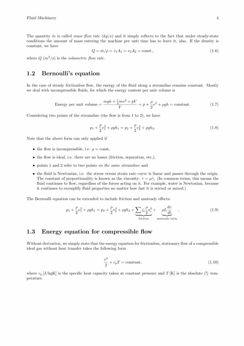
The quantity m is called mass flow rate (kg/s) and it simply reflects to the fact that under steady-stateconditions the amount of mass entering the machine per unti time has to leave it, also. If the density isconstant, we have

Q = m/ρ = v1A1 = v2A2 = const., (1.6)

where Q (m3/s) is the volumetric flow rate.

1.2 Bernoulli’s equation

In the case of steady frictionless flow, the energy of the fluid along a streamline remains constant. Mostlywe deal with incompressible fluids, for which the energy content per unit volume is

Energy per unit volume =mgh+ 1

2mv2 + pV

V= p+

ρ

2v2 + ρgh = constant. (1.7)

Considering two points of the streamline (the flow is from 1 to 2), we have

p1 +ρ

2v2

1 + ρgh1 = p2 +ρ

2v2

2 + ρgh2. (1.8)

Note that the above form can only applied if

• the flow is incompressible, i.e. ρ = const,

• the flow is ideal, i.e. there are no losses (friction, separation, etc.),

• points 1 and 2 refer to two points on the same streamline and

• the fluid is Newtonian, i.e. the stress versus strain rate curve is linear and passes through the origin.The constant of proportionality is known as the viscosity: τ = µγ. (In common terms, this means thefluid continues to flow, regardless of the forces acting on it. For example, water is Newtonian, becauseit continues to exemplify fluid properties no matter how fast it is stirred or mixed.)

The Bernoulli equation can be extended to include friction and unsteady effects:

p1 +ρ

2v2

1 + ρgh1 = p2 +ρ

2v2

2 + ρgh2 +∑

ζiρ

2v2i︸ ︷︷ ︸

friction

+ ρLdv

dt︸ ︷︷ ︸unsteady term

. (1.9)

1.3 Energy equation for compressible flow

Without derivation, we simply state that the energy equation for frictionless, stationary flow of a compressibleideal gas without heat transfer takes the following form

v2

2+ cpT = constant, (1.10)

where cp [J/kgK] is the specific heat capacity taken at constant pressure and T [K] is the absolute (!) tem-perature.

Fluid Machinery 5

1.4 Thermodynamics

1.4.1 Specific heat capacities

Assume that a definite mass of gas m is heated from T1 to T2 at constant volume and thus its internal energyis raised from U1 to U2. We have

mcV ∆T = ∆U or cV ∆T = ∆u, (1.11)

where u is the internal energy per unit mass and cV (J/(kgK)) is the specific heat capacity measured atconstant volume.

Now we do the same experiment but now at constant pressure, thus its volume changes and work is done onthe fluid:

mcp ∆T = ∆U +mp∆V, (1.12)

which, after rewriting for unit mass and combining with the previous equation for constant volume process,gives

cp ∆T = ∆u+ p∆V = cV ∆T +R∆T → cp = R+ cV . (1.13)

Thus we see that it is useful to define a new quantity which includes both the change of the internal energyu and the pressure work p dv = p d (1/ρ). Some useful equations:

R = cp − cV , κ =cpcV, cp = R

κ

κ− 1and cV = R

1

κ− 1. (1.14)

1.4.2 Some basic thermodynamic relationships

One possible form of the energy equation for a steady, open system in differential form is

δY + δq = d

(h+

c2

2+ gz

)︸ ︷︷ ︸

e

, (1.15)

δY is the elementary shaft work, δq is the elementary heat transferred towards the fluid, both of them beingprocesses, which is emphasised by the δ symbol. And

e = h+c2

2+ gz

is the energy. Note that the above equation describes an elementary process, however, to compute the overallprocess (to integrate the above equation), one has to know what kind of process takes place in the machine(adiabatic, isentropic, isotherm, etc.) and the results depends on it (thus, the integral is inexact).

The term enthalpy is often used in thermodynamics. It expresses the sum of the internal energy u and theability to do hydrodynamic work p

h = u+p

ρ. (1.16)

Note that h = cpT and u = cV T . There are some forms of expressing the change in enthalpy (v = 1/ρ):

dh = d(u+ pv) = δq + vdp = Tds+ vdp. (1.17)

Fluid Machinery 6

The entropy1 is for an elementary change in the equilibrium is

ds =δq

T+ dsirrev, (1.18)

with which, using (1.17) we obtain

dh = δq + Tdsirrev + vdp, (1.19)

with which (1.15) turns into

δY = vdp+ d

(c2

2+ gz

)︸ ︷︷ ︸

δYu(seful)

+Tdsirrev.︸ ︷︷ ︸losses

(1.20)

1.4.3 Input shaft work and useful work

The input shaft power is simply the work needed to change the enthalpy of the fluid:

Pin = m∆e = m

(h2 − h1 +

c22 − c212

+ g(z2 − z1)

)∣∣∣∣z1≈z2,c1≈c2

= mcp (T2 − T1) (1.21)

When computing the useful work, we integrate the Yu part of (1.20) between points 1 and 2 (e.g. betweenthe suction and pressure side of a compressor). We still assume that z1 ≈ z2 and c1 ≈ c2.

In the case of an isentropic process, we have p/ρ = RT (ideal gas law) and p/ρκ = const. (κ is the isentropicexponent), thus

Yisentr. =

∫ 2

1

p1/κ1

ρ1p−1/κdp =

p1/κ1

ρ

∫ 2

1

p−1/κdp =κ

κ− 1

p1

ρ1

[(p2

p1

)κ−1κ

− 1

]. (1.22)

Note that the above equation gives

Yisentr. =κ

κ− 1

p1

ρ1︸︷︷︸RT1

(p2

p1

)κ−1κ

︸ ︷︷ ︸T2/T1

−1

=κ

κ− 1R︸ ︷︷ ︸

cp

(T2 − T1) , (1.23)

which is exactly the input specific work defined by (1.21).

A typical compression system consists of a compressor and a pressure vessel, which stores the compressedgas. Although the gas heats up during the compression but in the vessel it will cool back to the pressure ofthe surroundings. In other words, we loose the heat energy and the ’useful’ process is isotherm. We havep/ρ = RT (ideal gas law) and T =const., thus

Yisotherm =p1

ρ1

∫ 2

1

1

pdp = RT1 ln

(p2

p1

)(1.24)

The real processes are usually described by polytropic processes but formally we use the same equationsas in the isentropic case, with the slight change of using the polytropic exponent n instead of κ. We have

1Entropy is the only quantity in the physical sciences that seems to imply a particular direction of progress, sometimes calledan arrow of time. As time progresses, the second law of thermodynamics states that the entropy of an isolated system neverdecreases. Hence, from this perspective, entropy measurement is thought of as a kind of clock.

Fluid Machinery 7

p/ρ = RT (ideal gas law) and p/ρn =const., thus∫ 2

1

1

ρdp

∣∣∣∣polytropic

=n

n− 1

p1

ρ1

[(p2

p1

)n−1n

− 1

]=

n

n− 1R (T2 − T1) . (1.25)

Polytropic processes are real, non-adiabatic processes. Note that the polytropic exponent n is typically aresult of curve fit that allows the accurate computation of the outlet temperature.

Finally, if the fluid is incompressible, we have

Yincomp. =1

ρ

∫ 2

1

1 dp =p2 − p1

ρ. (1.26)

1.4.4 Specific work for hydraulic machines

In the case of pumps, the fluid can be considered as incompressible. However, instead of Y usually the headis used:

H =Yug

=p2 − p1

ρg+c22 − c21

2g+ z2 − z1. [m] =

[J

N

](1.27)

In the case of ventilators, the energy change due to the geodetic heigth difference between the suction andpressure side is neglegible (z2 ≈ z1) and usually the change of total pressure is used:

∆pt = Yuρ = p2 − p1 + ρc22 − c21

2= pt,2 − pt,1. [Pa] =

[J

m3

](1.28)

In the case of compressors, the fluid cannot be considered as incompressible. When neglecting the losses,the specific work is:

Yu,isentropic = cp (T2s − T1) +c22 − c21

2= h2s,t − h1,t. (1.29)

1.4.5 Efficiency

The ratio of the useful power and the input power is efficiency. For a given T2 compression final temperature,we have

ηisentropic =T2s − T1

T2 − T1, (1.30)

for a polytropic process, we have

ηpolytropic =nn−1R(T2 − T1)

cp(T2 − T1)=

n

n− 1

κ− 1

κ. (1.31)

1.5 Problems

Problem 1.5.1

Fluid Machinery 8

The turbomachines conveying air are classified usually as fans (p2/p1 < 1.3), blowers (1.3 < p2/p1 < 3) andcompressors (3 < p2/p1). Assuming p1 = 1 bar inlet pressure, t1 = 20o C inlet temperature and isentropicprocess (κ = 1.4), find the the relative density change (ρ2−ρ1)/ρ1 at the fan-blower border and the t2 outlettemperature at the blower-compressor border. (Solution: (ρ2 − ρ1)/ρ1 = 20.6%, t2 = 128.1o C)

Problem 1.5.2

Assuming isentropic process of an ideal gas, find the inlet cross section area and the isotherm useful powerof a compressor conveying m = 3 kg/s mass flow rate. The velocity in the inlet section is c = 180 m/s.The surrounding air is at rest with p0 = 1 bar and T0 = 290 K. cp = 1000J/kgK, κ = 1.4. (Solution:A1 = 0.016 m2, Pisoth,u = 446.5 kW)

Problem 1.5.3

Gas is compressed from 1 bar absolute pressure to 3 bar relative pressure. The gas constant is 288J/kgK, thespecific heat at constant pressure is cp = 1005J/kgK. The exponent describing the politropic compression isn = 1.54. Find the isentropic exponent. Find the isentropic specific useful work, the specific input work andthe isentropic efficiency. The density of atmospheric air is 1.16 kg/m3. ht ≈ h is a reasonable approximation.(Solution: κ = 1.402, Yisentropic = 146.729 kJ/kg, Yinput = 188.289 kJ/kg, ηisentropic = 77.9%.)

Problem 1.5.4

Ideal gas (gas constant R = 288 J/kgK) with 27oC and 1 bar pressure is compressed to 3 bar with compressor.The exponent describing the real state of change is n = 1.5. Find the absolute temperature and density of theair at the outlet. Find the isentropic outlet temperature, the isentropic efficiency and the isentropic usefulspecific work. Find the power needed to cover the losses, if the mass flow is 3 kg/s. (Solution: Treal = 432.7K,ρ = 2.407 kg/m3, Tisentropic = 410.6K, ηisentropic = 83.3%, Yisentropic = 111.48 kJ/kg, Ploss = 66.8kW)

Problem 1.5.5

Gas is compressed from 1 bar to 5 bar. The ambient air temperature at the inlet T1 = 22◦C while at theoutlet T2 = 231◦C. Gas constant R = 288 J/kgK. Find the exponent describing the politropic compressionand the density of air at the inlet and the outlet. (Solution: n = 1.5, ρ1 = 1.177kg/m3, ρ2 = 3.44kg/m3.)

Problem 1.5.6

Along a natural gas pipeline compressor stations are installed L = 75 km distance far from each other. Onthe pressure side of the compressor the pressure is pp = 80 bar, the density is ρ = 85 kg/m3, while thevelocity of the gas is vp = 6.4 m/s. The diameter of the pipe is D = 600 mm the friction loss coefficient isλ = 0.018. Assuming that the process along the pipeline is isotherm, the pressure loss is calculated

asp2beg−p

2end

2 = pbegλLDρbeg

2 v2beg.

• Find the pressure, the density, and the velocity at the end of pipeline.

• Find the mass flow through the pipeline.

• Find the needed compressor power assuming that the compression is a politropic process and n = 1.45.

Fluid Machinery 9

• Find the ratio of the compressor power and the power that could be released by the complete combustionof the transported natural gas. The heating value of the natural gas is H = 43 MJ/kg. (Hint:Pcomb = mH)

(Solution: ps = 11.54 bar, ρs = 12.26 kg/m3, vs = 44.4 m/s, m = 153.8 kg/s, Pcomp = 38.42 MW, Pcomp/Pcomb =0.58%)

Chapter 2

Incompressible turbomachinery

We classify as turbomachines all those devices in which energy is transferred either to, or from, a continuouslyflowing fluid by the dynamic action of one ore moving blase rows. Essentially, a rotating blade row, a rotoror an impeller changes the stagnation enthalpy of the fluid moving through it. These enthalpy changes areintimately linked with the pressure changes in the fluid.

Up to 20% relative density change, also gases are considered to be incompressible. Assuming isentropicprocess and ideal gas, this corresponds to p2/p1 ≈ 1.3. Thus, pumps, fans, water and wind turbines areessentially the same machines.

2.1 Euler’s turbine equation

Euler’s turbine equation (sometimes called Euler’s pump equation) plays a central role in turbomachineryas it connects the specific work Y and the geometry and velocities in the impeller. In what follows, we givetwo derivations of the equation.

Figure 2.1: Generalized turbomachine

Derivation 1: Moment of momentum

Let us compute the moment of the force that is applied at the inlet and outlet of the generalized turbomachine

10

Fluid Machinery 11

shown in figure 2.1 :

F =d

dt(mc) → M =

d

dt(r ×mc) = m (r × c) (2.1)

where m is the mass flow, and c is the velocity of the fluid on the radius r. We consider the followingassumptions:

• The inlet of the turbomachine is a circle with radius r1, and the outlet with radius r2.

• c velocity is considered constant in the sense that its length and angle are constant.

ThusM = Mout −M in = m (r2 × c2)− m (r1 × c1)

. With this the power need of driving the machine is

mY = P = ωM = (Mout −M in) ω = m [ω (r2 × c2)− ω (r1 × c1)] (2.2)

= m [c2 (ω × r2)− c1 (ω × r1)] = m [c2u2 − c1u1] (2.3)

= m [|c2||u2| − |c1||u1|] = m (c2uu2 − c1uu1) (2.4)

where ui = |ui|, and ci = |c2u|cos(α) Comparing the beginning and the end of the equation, we see that thespecific work is

Y = c2uu2 − c1uu1 . (2.5)

Derivation 2: Rotating frame and reference and rothalpy

The Bernoulli equation in a rotating frame of reference reads

p

ρ+w2

2+ U = const., (2.6)

where U is the potential associated with the conservative force field, which is the potential of a rotatingframe fo refernce: U = −r2ω2/2. Let w stand for the relative velocity, c for the absolute velocity and u = rωfor the ’transport’ velocity. We have c = u+ w, thus w2 = u2 + c2 − 2u c = u2 + c2 − 2u cu, which gives

p

ρ+w2

2− r2ω2

2=p

ρ+c2 + u2 − 2cu

2− u2

2=p

ρ+c2

2− c u︸︷︷︸

cuu

= const. (2.7)

Thus we see that the above quantity is conserved in a rotating frame of reference, which we refer to asrothalpy (abbreviation of rotational enthalpy). Let us find now the change of energy inside the machine:

Y = ∆

(p

ρ+c2

2

)= ∆ (cuu) , (2.8)

which is exactly Euler’s turbine equation. (For compressible fluids, rothalpy is I = cpT + c2

2 − ucu.)

2.2 Velocity triangles and performance curves

IDE SZERINTEM KENE EGY HAROMSZOG

From the Euler turbine equation we have:

∆pe = ρgH = ρ (c2uu2 − c1uu1)

Fluid Machinery 12

where H is the head of the pump. Known the velocity triangle’s components and the density of the fluid,we get:

H =c2uu2 − c1uu1

g(2.9)

The flow rate isQ = c2mA2 = c2mD2πb2, (2.10)

where D2 is the impeller outer diameter, b2 is its flow-through width at the outlet. From 2.9 and 2.10 wehave that c outlet absolute velocity is the connection between the head and the flow rate of the pump. Alsoone can notice, that if ∆pe increased, that is when c2u is increased than Q decreases (c2m decreases). Andif ∆pe decreased (c2u decreased) than Q increases (c2m increases). So our goal now is to find a relationshipbetween the head and the flow rate of the pump.

2.2.1 Radial (centrifugal) machines

Let us consider a centrifugal pump and the velocity triangles at the impeller inlet and outlet, see Fig. 2.2.The theoretical flow rate is

Qth = c2mA2Ψ = c2mD2πb2Ψ, (2.11)

where D2 is the impeller outer diameter, b2 is its flow-through width at the outlet and c2m is the radialcomponent of the outlet absolute velocity. Ψ < 1 is a constant called blockage factor that takes into accountthat the real flow through area is smaller due to the blockage of the blade width at the outlet.

Figure 2.2: Centrifugal pumps

The velocity triangle describes the relationship between the absolute velocity c, the circumferential velocityu and the relative velocity w. Obviously, we have ~c = ~u+ ~w. Moreover, we know that (a) the circumferentialvelocity is u = Dπn and that (b) the relative velocity is tangent to the blade, i.e. the angle between u andw is approximately the blade angle β.

Basic trigonometrical identities show that c2u = u2 − c2m/ tanβ2. It is usual to assume that the flow hasno swirling (circumferential) component at the inlet (due to Helmholtz’s third theorem). In the reality, the

Fluid Machinery 13

Figure 2.3: Centrifugal impeller with outlet velocity components.

outlet flow angle is not exactly β2, thus the head is decreased, which is taken into account with the help ofthe slip factor λ (sometimes denoted by σ in the literature).

If there is no prerotation (i.e. c1u = 0), we have

Hth = λc2uu2

g= λ

(u2

2

g− u2

g

w2u

g

)= λ

(u2

2

g− u2

g

c2mtanβ2

)= λ

(u2

2

g− u2

g tanβ2D2πb2ΨQth

). (2.12)

Thus, the theoretical performance curve Hth(Qth) of a centrifugal machine is a straight line, which is (seeFigure 2.4)

• decreasing as Q is increased, for backward curved blades, i.e. β2 < 90o,

• horizontal, for radial blades (β2 = 90o) and

• increasing (as Q is increased) for forward curved blades, i.e. β2 > 90o.

2.2.2 Problems

Problem 2.2.7

A radial impeller runs at n=1440/min revolution speed and conveys Q = 40 l/s of water. The diameter ofthe impeller is D = 240 mm, the outlet width is b2 = 20 mm. The blade angle at the outlet is β2 = 25degrees. The inlet is prerotation-free. Find the theoretical head and draw a qualitatively proper sketch ofthe velocity triangle at the outlet. (Solution: Hth = 22.9m)

Problem 2.2.8

Fluid Machinery 14

Figure 2.4: Effect of blade shapes β2 angle on the performance curve.

The mean meridian velocity component of a radial impeller with D2 = 400 mm diameter at n = 1440rpmrevolution speed is cm = 2.5 m/s. The angle between the relative and circumferential velocity componentsis β2 = 25 degrees. With a geometrical change of the blade shape, this angle is increased to to 28 degrees,that results in 10% drop of the meridian velocity component. The inlet is prerotation-free. Find the relativehead change. (Solution: (H25o −H28o)/H25o = 4.6%)

2.2.3 Axial machines

In the case of axial machines the flow leaves the impeller axially, see Fig. 2.5. The flow-through area is(D2o −D2

i

)π/4, where Do and Di stand for the outer and inner diameter of the lade, respectively. Notice

that in this case, u1 = u2 because it is assumed that the flow moves along a constant radius. Assuming(again) prerotation-free inlet (c1u = 0), we have c2m = c1 (due to continuity).

Figure 2.5: Axial pump (left) and axial fan (right)

However, an important difference between axial and centrifugal pumps (fans) is that in the case of axialmachines, the the pressure rise changes along the radial coordinate of the blade:

∆pt(r) = ρu(r) (c2u(r)− c1u(r))|c1u=0 = ρ (2rπn)

(2rπn− c2m

tanβ2

). (2.13)

Thus, if we wanted to obtain constant ∆pt along the radial coordinate, the change of the circumferentialvelocity has to be compensated by varying β2.

Fluid Machinery 15

Figure 2.6: Axial impeller with outlet velocity components.

The twisted airfoil (aerofoil) shape of modern air-

Figure 2.7: World War I wooden propeller

craft propellers was pioneered by the Wright broth-ers. While both the blade element theory andthe momentum theory had their supporters, theWright brothers were able to combine both theo-ries. They found that a propeller is essentially thesame as a wing and so were able to use data col-lected from their earlier wind tunnel experimentson wings. They also found that the relative angleof attack from the forward movement of the aircraftwas different for all points along the length of theblade, thus it was necessary to introduce a twistalong its length. Their original propeller blades areonly about 5% less efficient than the modern equiv-alent, some 100 years later. (Source: Wikipedia)

2.2.4 Problems

Problem 2.2.9

The outer diameter of a CPU axial cooler ventilator is Do = 47 mm the inner diameter is Di = 21.5 mm therevolution speed is n = 2740 rpm. Due to the careful design the hydraulic efficiency is ηh = 85% howeverthe volumetric efficiency as consequence of leakage flow rate between the housing and the impeller is justηvol = 75%. The blade angle at the suction side is β1 = 20◦ while at the pressure side β2 = 40◦. Find theflow rate and the total pressure rise on the impeller. The density of the air is ρ = 1.25 kg/m3. Draw thevelocity triangles at the inlet and the outlet at the mean diameter.

• Aring =(D2

o−D2i )π

4 = 0.00137 m2

• Dmean = Do+Di2 = 0.03425 m

• umean = u1 = u2 = Dmeanπn = 4.913 ms

• cax = c1,ax = c2,ax = u tanβ1 = 1.788 ms

Fluid Machinery 16

• q = ηvolAringcax = 0.00184 m3

s

• w2u = caxtan β2

= 2.131 ms

• ∆cu = u− q2u = 2.782 ms

• ∆ptotal,ideal = ρu∆cu = 17.1 Pa

• ∆ptotal = ηh∆ptotal,ideal = 14.5 Pa

Problem 2.2.10

The inner diameter of an axial impeller is Di = 250 mm, while the outer one is Do = 400mm. The revolutionnumber of the impeller is 1470rpm. The inlet is prerotation-free. At Q = 0.36 m3/s the hydraulic efficiencyis 85%, the head is 6 m. The specific work along the radius is constant. Find the angles β1,2 at the innerand outer diameter. (Solution: β1,i = 13.7, β2,i = 16.7, β1,o = 8.7 and β2,o = 9.4 degrees)

Fluid Machinery 17

2.2.5 Real performance curves

Our analysis so far assumed that the flow inside the impeller is ideal (no losses) and that the streamlinesare following the blade shape (thus, blade angles are also the streamline angles). However neither of theseassumptions are true.

There are significant friction losses inside the impeller, the narrower the flow passage is, the higher thefriction losses will be. Moreover, the volute also introduces friction losses. These losses are proportional tothe velocity squared, thus H ′friction ∝ Q2.

On the other hand, if the angle of attack deviates from the ideal one, one experiences separation on the twosides of the blade. This is illustrated in Figure 2.8 for a constant circumferential velocity u as the flow rateand thus the inlet velocity c is varied, the relative velocity w also varies. At the design flow rate Qd theangle of attack ideal. For small flow rates, we have separation on the suction side of the blade, while forlarger flow rates the separation is on the pressure side of the blade. Thus we have H ′separation ∝ (Q−Qd)2.

To obtain the real performance curve, one has to subtract the above two losses from the theoretical head:H = Hth(Q)−K1Q

2 −K2(Q−Qd)2, which is illustrated in 2.8. Note that at the design point and close toit, the friction losses are moderate and no separation occurs. For lower flow rates, the friction loss decreaseswhile separation increases. For higher flow rates, both friction and separation losses increase.

Figure 2.8: Friction and separation losses in the impeller.

Fluid Machinery 18

2.3 Losses and efficiencies

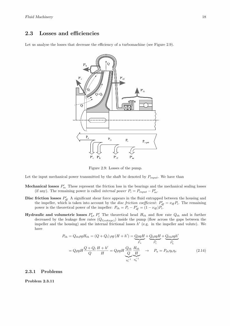
Let us analyse the losses that decrease the efficiency of a turbomachine (see Figure 2.9).

Figure 2.9: Losses of the pump.

Let the input mechanical power transmitted by the shaft be denoted by Pinput. We have than

Mechanical losses P ′m These represent the friction loss in the bearings and the mechanical sealing losses(if any). The remaining power is called internal power Pi = Pinput − P ′m.

Disc friction losses P ′df A significant shear force appears in the fluid entrapped between the housing andthe impeller, which is taken into account by the disc friction coefficient : P ′df = νdfPi. The remainingpower is the theoretical power of the impeller: Pth = Pi − P ′df = (1− νdf )Pi.

Hydraulic and volumetric losses P ′h, P′v The theoretical head Hth and flow rate Qth and is further

decreased by the leakage flow rates (Ql(eakage)) inside the pump (flow across the gaps between theimpeller and the housing) and the internal frictional losses h′ (e.g. in the impeller and volute). Wehave

Pth = QthρgHth = (Q+Ql) ρg (H + h′) = QρgH︸ ︷︷ ︸Pu

+QlρgH︸ ︷︷ ︸P ′v

+Qthρgh′︸ ︷︷ ︸

P ′h

= QρgHQ+QlQ

H + h′

H= QρgH

QthQ︸︷︷︸η−1v

Hth

H︸︷︷︸η−1h

→ Pu = Pthηhηv (2.14)

2.3.1 Problems

Problem 2.3.11

Fluid Machinery 19

The revolution number of a water pump is 1470 rpm, the flow rate is Q = 0.055m3/s and the head isH = 45m. The hydraulic power loss is P ′h = 2.5kW, the mechanical power loss is P ′m = 1.3kW, the discfriction coefficient is νt = 0.065. The input power at this operating point is Pin = 32kW. Make a completeanalysis of the losses, including leakage flow rate and the theoretical head.

Solution:

The power flow chart is: Pinput(P′m)→ Pi(P

′df )→ Pth(P ′v, P

′h)→ Pu(seful)

• Pi = Pinput − P ′m = 30.7 kW → ηm = 95.9%

• Pth = (1− ν)Pi = 28.7 kW

• h′h =P ′hρgQ = 4.63 m → Hth = 45 + 4.63 = 49.63 m → ηhydr = 90.6%

• Qth = PthρgHth

= 0.0589 m3/s → Qleakage = 0.00395 m3/s → ηv = 93.2%

• ηoverall = ηv · ηh · (1− ν) · ηm = 75.9%

Fluid Machinery 20

2.4 Dimensionless numbers and affinity

Based on the previously obtained formulae for theoretical head, we define dimensionless numbers as

H = ηhHth = 2ηhc2uu2

u22

2g:= ψ

u22

2g(2.15)

or, in the case of fans

∆pt = ψρ

2u2

2, (2.16)

where ψ is a dimensionless pressure rise. Similarly, we have

Q = ηvQth = ηvD2πb2c2m = ηv4D2πb2

4D22

c2mu2

u2D22 := ϕ

D22π

4u2 (2.17)

These dimensionless quantities are called pressure number ψ and flow number ϕ. What we found is thatH ∝ n2 and Q ∝ n allowing the transformation of the performance curve given at n1 to be computed toanother revolution number n2. This is called affinity law :

H1

H2=

(n1

n2

)2

,Q1

Q2=n1

n2→ P1

P2=

(n1

n2

)3

(2.18)

As we have seen, both ψ and ϕ contains two parameters, D2 and u2, out of which one can be eliminated,resulting in new dimensionless numbers. Let us start with the elimination of D2.

ϕ =Q

D22π4 u2

=4Q

D32π

2n(2.19)

ψ =Hu22

2g

=2gH

D22π

2n2(2.20)

from which we have

σ =ϕ1/2

ψ3/4=

2√Q

D3/22 π√n

D3/22 π3/2n3/2

(2gH)3/4

=

√π

4√

2g3/4nQ1/2

H3/4︸ ︷︷ ︸nq

(2.21)

Note that σ depends only on the revolution number but takes different values along the performance curve.Thus when actually computing it, one takes the data of the best-efficiency point. Moreover, we do not

include the constant term√π

4√2g3/4. Finally, by definition, the specific speed of a turbomachine is

nq = n[rpm]

(Qopt.[m

3/s])1/2

(Hopt.[m])3/4

(2.22)

Specific speed defines the shape of the impeller, low specific speed means low flow rate and high pressurerise (radial impeller) while high specific speed occurs when the flow rate is high and the pressure rise is low,see Fig. 2.10.

Based on experience the available maximum efficiency can be estimated in the knowledge of Qopt and nq asfollows

ηmax = 0.94− 0.048Q−0.32opt − 0.29

(log(nq

44

))2

. (2.23)

Representing δopt(σopt), turbomachines having good efficiency pass a narrow path. This diagram is calledCordier-diagram. The centre of the path can be assumed with

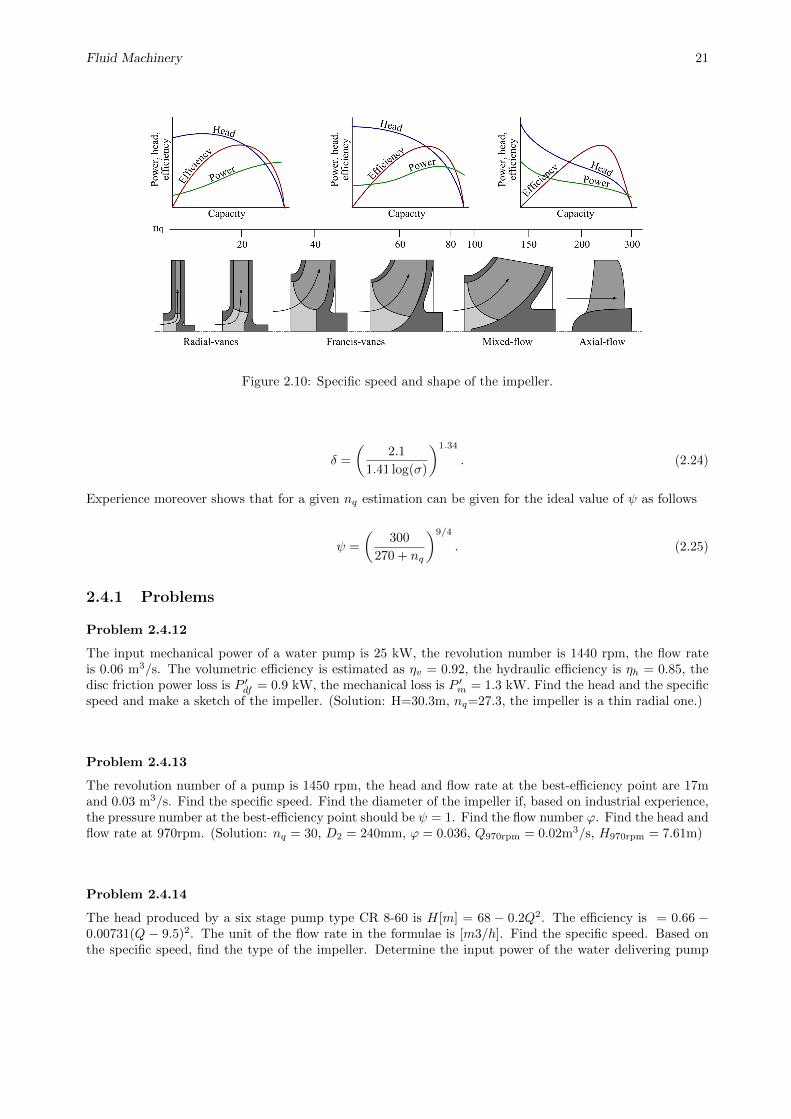
Fluid Machinery 21

Figure 2.10: Specific speed and shape of the impeller.

δ =

(2.1

1.41 log(σ)

)1.34

. (2.24)

Experience moreover shows that for a given nq estimation can be given for the ideal value of ψ as follows

ψ =

(300

270 + nq

)9/4

. (2.25)

2.4.1 Problems

Problem 2.4.12

The input mechanical power of a water pump is 25 kW, the revolution number is 1440 rpm, the flow rateis 0.06 m3/s. The volumetric efficiency is estimated as ηv = 0.92, the hydraulic efficiency is ηh = 0.85, thedisc friction power loss is P ′df = 0.9 kW, the mechanical loss is P ′m = 1.3 kW. Find the head and the specificspeed and make a sketch of the impeller. (Solution: H=30.3m, nq=27.3, the impeller is a thin radial one.)

Problem 2.4.13

The revolution number of a pump is 1450 rpm, the head and flow rate at the best-efficiency point are 17mand 0.03 m3/s. Find the specific speed. Find the diameter of the impeller if, based on industrial experience,the pressure number at the best-efficiency point should be ψ = 1. Find the flow number ϕ. Find the head andflow rate at 970rpm. (Solution: nq = 30, D2 = 240mm, ϕ = 0.036, Q970rpm = 0.02m3/s, H970rpm = 7.61m)

Problem 2.4.14

The head produced by a six stage pump type CR 8-60 is H[m] = 68 − 0.2Q2. The efficiency is = 0.66 −0.00731(Q − 9.5)2. The unit of the flow rate in the formulae is [m3/h]. Find the specific speed. Based onthe specific speed, find the type of the impeller. Determine the input power of the water delivering pump

Fluid Machinery 22

for zero delivery Q = 0 by extrapolation from calculated points in the range Q = 1.5; 1; 0.5m3/h, and usingL’Hopital’s rule. (Solution: nq = 29.9, hence the impeller is radial; Pin = 1334W .)

Problem 2.4.15

The characteristic curve of a pump at n1 = 1450/min rotor speed is H1 = 40m−40000s2/m5Q2. Calculate 5points of the pump-characteristic for the rotor speed n2 = 2900/min in the flow rate range Q2 = 0, 01m3/s−0, 05m3/s at 0, 01m3/s intervals. According to laboratory tests the affinity law is valid in this range. Givethe equation of the characteristics H2(Q2) for the rotor speed n2! (Solution: H2(Q2) = 160− 40000Q2

2)

Problem 2.4.16

Find the specific speed of the pump given by 2.11, if the revolution number is 3000 rpm. Make a sketch ofthe impeller. (Solution: nq = 92, mixed impeller.)

Figure 2.11: Performance chart for Problem 2.4.16.

Problem 2.4.17

The performance curve of a pump at 1450 rpm is given by H = 100 − 30000Q2 and the efficiency is givenby η = −78000Q2 + 4500Q. Find the head and flow rate of the best-efficiency point. Find the performancecurve at 1740 rpm. (Hopt = 76m, Qopt = 0.02855m3/s, etamax = 64.9%, H1740rpm = 144− 30000Q2.)

Fluid Machinery 23

2.5 Forces on the impeller

2.5.1 Radial force

TODO

2.5.2 Axial force

The axial force results from two components:

• Momentum force

• Pressure distribution on the hub and shroud.

The momentum force isFm = mv = ρr2

1πc21, (2.26)

Figure 2.12: Pressure distribution on the hub.

The pressure distribution is

p(r) =ρ

2r2ω2

f +K p(R2) = p2 −∆p′2 → p(r) = p2 −∆p′2 −ρ

2ω2f

(r22 − r2

). (2.27)

The axial force becomes, e.g. on the hub (back of the impeller)

Fhub =

∫ r2

rs

2rπp(r)dr = · · · =(r22 − r2

s

)π

(p2 −∆p′2 −

ρ

2ω2f

r22 − r2

s

2

). (2.28)

A similar result is obtained for the shroud (front of the impeller) with replacing rs by r1. The overall axialforce is

Fax = Fhub − Fshroud − Fm, (2.29)

and its direction is towards the suction side (the axial force tries to ’pull down’ the impeller from the shaft).

TODO: Extend explanations.

Fluid Machinery 24

2.6 Problems

Problem 2.6.18

Find the axial force on the back of the impeller, whose outer diameter is D2 = 300mm, the shaft diameteris Ds = 50mm, the outlet pressure is 2.3bar and the revolution number is 1470rpm. The average angularvelocity of the fluid is 85% of that of the impeller. (Solution: F = 9.36kN)

Problem 2.6.19

Calculate the axial force acting on the supporting disc of a pump impeller of 280mm diameter if the pressureat the impeller exit is 2bar. The hub diameter is 40mm. There is no leakage flow through the gap between therotor supporting disc and the casing. The rotor speed is 1440/min. The angular velocity of the circulatingwater is half of that of the rotor. Find the formula of pressure distribution as a function of the radialcoordinate! Draw the cross section of the impeller and the axial pressure force!

2.7 Cavitation

2.7.1 Problems

Problem 2.7.20

A pump delivers water from a low-pressure steam boiler as shown in the figure below. Calculate the requiredgeodetic height of the reservoir to avoid cavitation! The pipeline losses are to be taken into account.

• mass flow rate: m = 27[kg/s], density of the hot wa-ter: ρ = 983[kg/m3]

• pipe: L = 10[m], d = 100[mm], λ = 0.02 and the sumof loss factors is ζ = 5

• pump: H[m] = 82 − 4800Q2, NPSH[m] = 1.6 +13600Q2

Solution:It’s easy to calculate thatQ = m/ρ = 0.02747[m3/s]cs = Q/A = 3.5[m/s]H = 82− 4800× 0.027472 = 78.38[m]NPSH = 1.6 + 13600× 0.027472 = 2.626[m]

Bernoulli’s equation between a surface point in the tank and the suction side of the pump reads:

ptρg

+02

ρg+Hs =

psρg

+c2sρg

+ 0 + h′pipeline

From the suction side of the pump to the impeller we have:

psρg

+c2s2g

=pvapourρg

+ es +NPSH

Fluid Machinery 25

(Note that es = 0 as the configuration is horizontal.) Putting the above two equations together, we have

Hs = −pt − pvapourρg

+ h′pipe +NPSH, where h′pipe =c2s2g

(λ

Hs + L

d+ ζ

),

thus,

Hs =

(1 +

c2s2g

λ

d

)−1 [NPSH +

c2s2g

(λL

d+ ζ

)]= · · · = 6.42[m]

Thoma’s cavitation coefficient is σ = NPSH/H = 0.03355[−].

Problem 2.7.21

Calculate the required pipe diameter to avoid cavitation, if the pump delivers Q = 30 dm3/s water from aclosed tank, where the pressure (above the water level) is p = 40 kPa. The equivalent pipe length on thesuction side is 5m, the friction coefficient is λ = 0.02, the suction flange of the pump is 3 m below the waterlevel. The vapour pressure at the water temperature is 2.8 kPa. The required net positive suction head isNPSHr = 3.2 m. (The standard pipe diameter series is: DN 40, 50, 65, 80, 90)

Solution:

The sketch of the installation is shown in Figure 2.13

Figure 2.13: Installation of the apparatus.

• NPSHa = pt−pvρg −Hs − h′s → h′s = pt−pv

ρg −Hs −NPSHr

• h′s = λ LeDsc2s2g = λ LeDs

8Q2

D5sgπ

2

• Ds = 0.073m→ Ds = 80 mm

Problem 2.7.22

Find the required suction side height of the pump that conveys water from an open surface reservoir atQ = 180m3/h flow rate the head is H = 30m the required net positive suction head NPSHr = 5.03m.The temperature of the water is T = 23◦ the ambient pressure is p0 = 1023mbar. The hydraulic loss ofthe suction side pipe can be calculated from h′s = 652[s2/m5]Q2 while the vapour pressure pv = 1.704 +0.107(t− 15) + 0.004(t− 15)2. Find the Thoma cavitation number. (Solution: Hs = 3.481m, σ = 0.154)

Chapter 3

Hydraulic Systems

3.1 Frictional head loss in pipes

In hydraulic machinery, instead of pressure p [Pa], usually the term head is used: H [m] = pρg . In real

moving fluids, energy is dissipated due to friction, as well as turbulence. Note that as the hydraulic poweris P = ρgHQ, but - because of the continuity equation - the flow rate is constant, the energy loss manifestsitself in head (pressure) loss. Head loss is divided into two main categories, ”major losses” associated withenergy loss per length of pipe, and ”minor losses” associated with bends, fittings, valves, etc. The mostcommon equation used to calculate major head losses is the Darcy Weisbach equation:

h′f = λL

D

v2

2g= λ

L

D

8Q2

D4π2, (3.1)

where the friction coefficient λ (sometimes denoted by f) depends on the Reynolds number (Re = vD/ν,ν [m2/s] = µ/ρ being the kinematic viscosity of the fluid) and the relative roughness e/D (e [m] being theroughness projections and D the inner diameter of the pipe). Based on Nikuradses experiments, we havedifferent regimes based on the Reynolds number.

• For laminar flow Re < 2300, we have λ = 64.

• For transitional flow 2300 < Re < 4000, the value of λ is uncertain and falls into the range of 0.03 . . . 0.08for commercial pipes.

• For turbulent flow in smooth pipes, we have 1√λ

= 1.95 log(Re√λ)−0.55. However, this equation need

iteration for computing the actual value of λ. Instead, in the range of 4000 < Re < 105, the Blasiussformula is ususllay used: λ = 0.316/ 4

√Re.

• For turbulent flow in rough pipes, Karman-Prandtl equation may be used: 1√λ

= −2 log(

e3.7D

)The

Colebrook-White equation covers both the smooth and rough regime: 1√λ

= −2 log(

1.88Re√λr

+ e3.7D

)For relatively short pipe systems, with a relatively large number of bends and fittings, minor losses can easilyexceed major losses. These losses are usually taken into account with the help of the loss factor ζ in theform of

h′ = ζρ

2v2. (3.2)

26

Fluid Machinery 27

In design, minor losses (ζ) are usually estimated from tables using coefficients or a simpler and less accuratereduction of minor losses to equivalent length of pipe (giving the length of a straight pipe with the samehead loss). Such relationships can be found in *[2], *[1] or *[3].

3.2 Head-discharge curves and operating point

Let us consider a single pipe with several elbows, fittings, etc. that ends up in a reservoir, see Figure 3.2.

Figure 3.1: Simple pumping system.

The head Hs(ystem) needed to convey Q flow rate covers the pressure difference and the geodetic heightdifference between the starting and ending point and the losses of the flow: the friction of the pipe, the lossof the elbows, valves, etc., and the discharge loss.

Hs(ystem) =p2 − p1

ρg+ (z2 − z1) +

(∑ζ +

∑λL

D+ 1

)v2

2g= Hstat +BQ2 (3.3)

where

• Hstat =p2 − p1

ρg+ (z2 − z1)

• B =(∑

ζ +∑λ LD + 1

) 8

D4π2g

Note

• Hstat is independent of the flow rate Q

•∑ζ denotes the loss of the elbows, valves, etc.

•∑λ LD stands for the frictional loss of the pipe

• +1 represents the discharge loss at index 2.

Fluid Machinery 28

3.3 Problems

Problem 3.3.23

Calculate the head loss of the pipe depicted in the figure below as a function of the volume flow rate!Parameters: ζA = 1.5, ζB,D = 0.26, ζC = 0.35, ζF = 0.36, λ = 0.0155, Ds = Dp = D = 0.6[m] andQ = 0.4[m3/s]. Solution:

• Static (geodetic) head + dynamic (friction) losses of the pipe: Hpipe = Hstat +Hfriction

• Volume flow rate: Q = cs(uction)Apipe,suction = cp(ressure)Apipe,pressure = cApipe

• The ’extra’ 1 in the pressure side (...ζD + 1) represents the outflow losses.

• Hstat = 8 + 4 = 12[m], Ls = 7 + 6 = 14[m], Lp = 12 + 20 + 8 = 40[m]

Hpipe = Hstat +KQ2 = Hstat +

[(λLsDs

+ ζA + ζB

)c2s2g

+

(λ

∑Lp

Dp+ ζF + ζC + ζD + 1

)c2p2g

]=

= 12[m] + 3.25[s2/m5]×Q2[m3/s]2

Problem 3.3.24

The artificial fountain Beneath the St. Gellert is fed by two pipelines of 30m length. The height distancebetween the pump and the fountain is 22m. The diameter of the pipes is D1 = 100mm and D2 = 70mm,the friction coefficient of the straight segments is λ = 0.02 and the friction coefficient of the other segments(bends, etc.) is ζ = 0.5. Assuming that the flow velocity in the first pipe is 1.5m/s, calculate the therequired head. Calculate the flow velocity in the second pipe and the overall flow rate of the common pumpfeeding the two pipes.Assuming 65% overall (pump+motor) efficiency, calculate the energy demand for 100days and the cost of the operation if the energy tariff is 32HUF/kWh. (Solution: Without the bypass line:H = 22.826m[], Q = 0.01678[m3/s], P = 5.78[kW ] and Cost = 443691HUF .)

Problem 3.3.25

Fluid Machinery 29

A pump delivers Q = 1200[dm3/min] water from an open-surface well, whose water level is 25[m] below thedefault level. The pressure side ends 5[m] above the default level and the water flows into an open-surfaceswimming pool. The diameter of the pipe on the suction side is Ds = 120[mm] and Dp = 100[mm] on thepressure side. The loss coefficients are ζs = 3.6 and ζp = 14 (without the outflow losses). Calculate therequired pump head! (Solution: Hp,req. = 35.7[m])

Problem 3.3.26

The submergible pump shown in the picture below delivers Q = 30l/s water into the basin. The pipecollecting the water of five equal pumps has a diameter D. The inner diameter of the pressure tube connectingthe pump with the collecting pipe is d. Find the head of the system and the pump head! Further data are:D = 400mm, λD = 0.018, d = 160mm, λd = 0.021, ζfilter = 3 , ζnrv = 0.25, ζbd = 0.35, ζ2bd = 0.5,ζbD = 0.22. (Solution: Hsystem = 11.07m, Hpump = 12.80m)

Chapter 4

Control

4.1 Problems

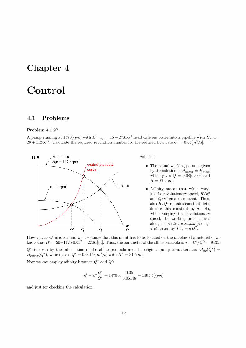
Problem 4.1.27

A pump running at 1470[rpm] with Hpump = 45− 2781Q2 head delivers water into a pipeline with Hpipe =20 + 1125Q2. Calculate the required revolution number for the reduced flow rate Q′ = 0.05[m3/s].

Solution:

• The actual working point is givenby the solution of Hpump = Hpipe,which gives Q = 0.08[m3/s] andH = 27.2[m].

• Affinity states that while vary-ing the revolutionary speed, H/n2

and Q/n remain constant. Thus,also H/Q2 remains constant, let’sdenote this constant by a. So,while varying the revolutionaryspeed, the working point movesalong the central parabola (see fig-ure), given by Hap = aQ2.

However, as Q′ is given and we also know that this point has to be located on the pipeline characteristic, weknow thatH ′ = 20+1125·0.052 = 22.81[m]. Thus, the parameter of the affine parabola is a = H ′/Q′2 = 9125.

Q∗ is given by the intersection of the affine parabola and the original pump characteristic: Hap(Q∗) =

Hpump(Q∗), which gives Q∗ = 0.06148[m3/s] with H∗ = 34.5[m].

Now we can employ affinity between Q∗ and Q′:

n′ = n∗Q′

Q∗= 1470× 0.05

0.06148= 1195.5[rpm]

and just for checking the calculation

30

Fluid Machinery 31

H ′ = H∗(n′

n∗

)2

= 34.5× 1195.52

14702= 22.81[m].

Problem 4.1.28

Solve the previous control problem (pump: Hpump = 45 − 2781Q2, pipeline: Hpipe = 20 + 1125Q2, desiredflow rate: Q′ = 0.05[m3/s]) using a throttle at the pressure side of the pump and also with a bypass line.Compare the resulting operations in terms of power loss!

Fluid Machinery 32

Problem 4.1.29

A pump, whose characteristic curve is given by Hpump = 70 − 90000[s2/m5]Q2, works together with twoparallel pipes. The main pipe is given by H1 = 30 + 100000[s2/m5]Q2. Calculate the head-flow relationshipH2(Q) of the side pipe, whose opening results in a flow rate of 480[l/min] in the main pipe. The static headof the second side pipe is 25[m].

Solution:

• Head of the main pipe at the prescribed flow rate: Q1 = 480[l/min] = 0.008[m3/s] → H1(Q1) =36.4[m]

• The head is the same, so the flow rate of the pump is Hp(Qp) = H1(Q1) → Qp =√

70−36.490000 =

0.0193[m3/s]

• Thus, the flow rate on the side pipe is Q2 = Qp −Q1 = 0.0193− 0.008 = 0.0113[m3/s]

• The actual characteristic of the side pipe: H2(Q2) = 25 + aQ22 = 36.4[m] → a = 36.4−25

0.01132 = 89279

• The solution is H2(Q2) = 25 + 89279Q2.

Problem 4.1.30

Pumps I and II feed pipes 1 and 2 shown in the figure below. Their characteristics are:

HI = 45m− 24900s2/m5Q2

HII = 35m− 32200s2/m5Q2

H1 = 10m− 4730s2/m5Q2

H2 = 15m− 8000s2/m5Q2

Find the flow rates and heads if valve ”V ” is closed, and if it it opened.

Problem 4.1.31

Two pumps, H1 = 70m − 50000s2/m5Q2 and H2 = 80m − 50000s2/m5Q2 can be coupled parallel or inseries. Which arragement will deliver more liquid through the pipe Hp = 20m+ 25000s2/m5Q2?

Problem 4.1.32

Fluid Machinery 33

Pump S, with the characteristitc curve HS = 37 − 0.159Q2, is feeding an irrigation system consisting ofparallel pipes. The units are Q[m3/h] and H[m]. Each pipe contains at its end a sprinkler. The pipes are20m long, their inner diameter is 25mm, the friction coefficient is 0.03. The sprinklers discharge 4m3/hwater at 2bar overpressure, their characteristics can be written as Hspr = KsprQ

2.

• Draw the sketch of the irrigation system with 3 parallel pipes!

• How much water is discharged if only one pipe is in operation?

• How many parallel pipes can be fed if the overpressure before the sprinklers must be 2bar?

Problem 4.1.33

The characteristics of a pump supplying a small village with water is Hp = 70− 330Q2. The village networkis modeled by the curve Hcd = 25 + 30Q2 during the day while the night operation can be described byHcn = 25 + 750Q2. A high water tower is attached to the delivery tube of the pump, its characteristics isHT = 40− 55|Q|Q. Here Q is positive if water flows down from the tower. The units in the formulae are [Q]= m3/s; [H] = m. Draw a sketch of the water system. Find the flow rates of the pump, village and towerboth for day and night operation. Find the head of the pump both for day and night! Use a millimeterpaper to draw the charasteristics curves! (Solutions: Qpump = 0.33m3/s and 0.29m3/s; Qvillage = 0.6m3/sand 0.15m3/s; Qtower = 0.275m3/s and −0.14m3/s. Hpump = 36m and 41m.)

Problem 4.1.34

How much water is delivered by the pump Hp = 70− 45000Q2 through the pipe system Hs = 20 + 20000Q2

? The flow rate must be reduced to 0.015m3/s. This can be done either by throttling control or by usinga by-pass control. Draw the pump-pipe-valve arrangements for both cases. How large is the hydraulicloss in the valves in the first and in the second case? The power consumption of the pump is Pinput =9.4 + 6240Q− 50000Q2. How large is the specific energy consumption f in the two cases? The units in theformulae are: [m], [m3/s], [kW ].

Chapter 5

Positive displacement pumps

5.1 Problems

Problem 5.1.35

Calculate the hydraulic power of the double-acting piston pump, which delivers water from an open-surfacetank into a closed one with 500[kPa] gauge pressure (i.e. relative pressure) located 50[m] above the suctiontank. Diameter of the piston is D = 120[mm], the stroke is 150[mm] and the driving motor runs at 120[rpm].

Solution:

Qmean = 2×Apiston × s× n = 2× 0.122π4 × 0.15× 120

60 = 6.78× 10−3[m3

s ]

∆p = ptank,abs. − p0 + ρgH = ptank,rel. + ρgH = 991[kPa]

P = Q∆p = 6.72[kW ]

Problem 5.1.36

The characteristic curve of a gear pump is Q[dm3/min] = 11.93 − 0.0043δp[bar]. The volumetric efficiencyat 35bar pressure difference is 92%. Find the volume flow rate and the geometric volume! The shaft speedis 80rev/min. How large is the driving torque if the pump efficiency is 85%?

Problem 5.1.37

The piston diameter of a hydraulic cylinder is 50mm. An 800kg load is lifted by the piston rod of 20mmdiameter with 12m/min velocity. How large must be the flow rate Q of the gear pump rotating withn = 960/min speed if its volumetric efficiency is 92%? Find the geometric volume of the pump and thepressure rise produced by it! Find the power P and the torque M of the driving motor! The pump efficiencyis 74%. Prepare a sketch of the gear pump showing the rotation direction of the shafts, intake and deliveryports! How large will be P , M , Q if the rotor speed is n = 1440/min?

Problem 5.1.38

The piston diameter of a vertical hydraulic cylinder is supporting a mass of 700kg. It may not be loweredfaster than 64mm/s. The cylinder diameter is 50mm, the piston rod diameter is 28mm. The pump deliverycurve is Q[liter/min] = 8.6−0.0467p[bar]. The hydraulic oil of 970kg/m3 density leaves the cylinder through

34

Fluid Machinery 35

a throttle valve. The discharge coefficient of this valve is = 0.7. Find the valve area at the maximal opening!

Chapter 6

Hydro- and wind power

6.1 Problems

Problem 6.1.39

The cross-section of a plant water channel is given. The measured average water depth is h = 2.9 m, thewidth of the channel is B = 25 m. The velocity of the water flow is measured at several locations of the cross-section using a cup-type anemometer. The calculated average velocity is v = 0.4 m/s. The height differencebetween the upstream and downstream water depth at the dam is hupstream − hdownstream = 4.5 m. Theefficiency of the turbine is ηturbine = 90 % the efficiency of the generator is ηgenerator = 96 %. The inputpower and useful power of the power plant are to be calculated. What is the value of the hydraulic radius?What type of turbine is suitable for this power plant?

Solution:

• A = hB = 72.5 m2

• Q = Av = 29 m3/s

• H = hupstream − hdownstream = 4.5 m

• P input = QρgH = 1.28 MW

• Puseful = ηturbineηgeneratorP input = 1.106 MW

• Rh = AreaPerimeter = Bh

2h+B= 2.35 m

Turbine type: Kaplan turbine.

Problem 6.1.40

The instantaneous efficiency of an existing wind turbine is to be calculated. The measured average windspeed at the level of the rotor is v1 = 12 m/s. The average speed of the air behind the rotor is v3 = 8 m/s.The diameter of the rotor is D2 = 55 m, the density of the air is ρair = 1.2 kg/m3. Find the calculatedefficiency related to the theoretical maximum of the efficiency?

Solution:

• ∆v = v1 − v3 = 4 m/s

36

Fluid Machinery 37

• A2 =D2

2π4 = 2376 m2

• P input = ρairA2v1v212 = 2.463 MW

• Puseful = ρairA2v31

(1− ∆v

2v1

)2∆vv1

= 1.140 MW

• η = CP =PusefulP input

= 0.463 < 1627 = 0.593

Problem 6.1.41

How large is the power of a wind turbine of 30m rotor diameter if the wind speed is 8m/s? The Betz limitof the power coefficient Cp is 0.593.