fluid antenna systems - arxiv
TRANSCRIPT

Fluid Antenna Systems‡
Kai-Kit Wong§, Arman Shojaeifard¶, Kin-Fai Tong§, and Yangyang Zhang‖
May 26, 2020
Abstract
Over the past decades, multiple antenna technologies have appeared in many different forms, most
notably as multiple-input multiple-output (MIMO), to transform wireless communications for extraor-
dinary diversity and multiplexing gains. The variety of technologies has been based on placing a number
of antennas at fixed locations which dictates the fundamental limit on the achievable performance. By
contrast, this paper envisages the scenario where the physical position of an antenna can be switched
freely to one of the N positions over a fixed-length line space to pick up the strongest signal in the
manner of traditional selection combining. We refer to this system as a fluid antenna system (FAS) for
tremendous flexibility in its possible shape and position. The aim of this paper is to study the achiev-
able performance of a single-antenna FAS system with a fixed length and N in arbitrarily correlated
Rayleigh fading channels. Our contributions include exact and approximate closed-form expressions for
the outage probability of FAS. We also derive an upper bound for the outage probability, from which
it is shown that a single-antenna FAS given any arbitrarily small space can outperform an L-antenna
maximum ratio combining (MRC) system if N is large enough. Our analysis also reveals the minimum
required size of the FAS, and how large N is considered enough for the FAS to surpass MRC.
Index Terms
Fluid antennas, MIMO, Multiple antennas, Selection combining, Outage.
‡The work is supported by EPSRC under grant EP/M016005/1.§Department of Electronic and Electrical Engineering, University College London, London, United Kingdom.¶BT Labs, Ipswich, United Kingdom.‖Kuang-Chi Institute of Advanced Technology, Shenzhen, China.
arX
iv:2
005.
1156
1v1
[cs
.IT
] 2
3 M
ay 2
020

I. Introduction
Wireless communications technologies have come a long way and there is never an absence of innovative
technologies when a new generation is introduced to succeed the current generation [1]. Nonetheless,
few would disagree that the most celebrated wireless technology over the past thirty years has to be
multiple-input multiple-output (MIMO). The phenomenon that MIMO can create bandwidth out of space,
independent of time and frequency resources, has shocked numerous researchers at the time and ever since
revolutionized wireless communications technologies via many forms, e.g., [2–10].
The earliest version of MIMO emerged in the patent by Paulraj and Kailath in 1994 [2] but it was
Foschini and Gans’ work in [3] that marked the beginning of MIMO research for years to come, as their
paper provided a theoretical argument, for the first time, that MIMO is capable of scaling up capacity with
the number of antennas at both ends. Around the same time, space-time codes by Tarokh et al. [4] and
Alamouti [5] further laid a solid foundation of MIMO. The intuition that multipath can boost capacity
performance was not easy to swallow at the time, and the capacity benefit of MIMO was only formally
characterized by introducing the notion of diversity and multiplexing gains by Zheng and Tse in 2003
[6]. Since then, MIMO has continued to influence the development of wireless communications technology,
taking the form of multiuser MIMO [7, 8] and massive MIMO being its latest version [9, 10].
The rationale behind MIMO is to exploit diversity over multiple signals at the antennas undergoing
independent fading, and the different fading signatures enabled by MIMO allow data to be multiplexed and
more data to be conveyed over wireless medium. Spatial correlation between antennas is understood to be
undesirable for spatial diversity of MIMO. At the mobile devices such as tablets and handsets, etc., the rule
of thumb has been to only deploy antennas with at least half-wavelength apart to have the full diversity
benefit. This rule may be justified by recognizing the fact that the correlation between two antennas with
separation d is expected to follow the Jake’s model [11], so that
J0
(2πd
λ
)= 0⇒ d =
(2.4
2π
)λ ≈ 0.38λ ≈ λ
2, (1)
where J0(·) is the zero-order Bessel function of the first kind, and λ is the wavelength of propagation.
Another reason why it is not advisable to fit antennas with less than half-wavelength apart is that when
antennas are too close, they start interacting in the near field, giving rise to coupling. In light of this, the
1

use of MIMO at mobile devices is greatly limited by the available space, not to mention the hardware cost
of an RF chain for each antenna that is added to the system.
Space at mobile devices is precious. Decades of effort have been devoted to designing antennas with high
gains, large bandwidth, and agility as well as a small form factor. Conventional antennas are mainly based
on metallic elements with high conductivity, strong mechanical stability, and demonstrated successes in
various reconfigurability [12]. Although antennas do get much smaller over the years, advances in antenna
technologies contribute only little to the massive deployment of antennas at the mobile side, as long as
the λ2 -rule remains. This paper argues that significant performance enhancement is possible even with
antennas located very close to each other in a tiny space. This can be comprehended by observing the
fading behaviour of the envelope of a typical received signal, as shown in Figure 1(a). The deeper the
fade, the shorter the displacement required to get out of the fade. As small as λ10 in space could make the
difference between at the bottom of a deep fade and a plateau of great reception.
All things considered, although it is not cost effective to deal with the complicated issue of mutual
coupling and fit many antennas within a small space for diversity, antennas at highly correlated spaces
do potentially benefit in the mitigation of fading. In this paper, we hypothesize a system where a single
antenna can switch locations instantly in a small linear space, and refer to this system as a fluid antenna
system (FAS) for its dynamic nature in possible shape and position. This paradigm is motivated by the
recent trend of using liquid metals such as Galinstan, Eutectic Gallium-Indium (EGaIn) and etc., or more
accessible ionized solutions such as sodium chloride (NaCl) and potassium chloride (KCl) for antennas,
e.g., [13–20]; see [21] for a review of liquid metal antennas. While this is very much a growing research
area, there is no doubt that software-controlled, mechanically flexible antennas are on their way.
Inspired by this, this paper considers that the FAS has N fixed locations (known as ‘ports’),1 evenly
distributed along a linear dimension of a given length, where the mechanically flexible antenna can always
be switched to the port with the strongest signal.2 Of particular relevance is the situation in which the
space making up the FAS is small but N can be very large, corresponding to the case that diversity is
obtained from a large number of spatially correlated ports. It is worth noting that mutual coupling is
not an issue in our model because only one antenna exists. The aim of this paper is to investigate the
1It is worth pointing out that a port in 3GPP normally means an antenna TXRU (RF chain) with a reference signal butfor the FAS, all ports share one single TXRU (RF chain).
2Note that while we are inspired by the research and use the term ‘fluid antenna’ in this paper, the results of our work arealso applicable to other flexible antenna structures such as software-controlled pixel antennas [22].
2
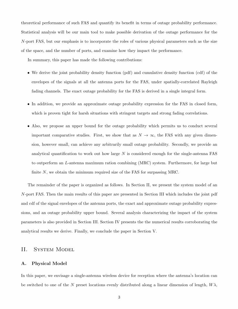
theoretical performance of such FAS and quantify its benefit in terms of outage probability performance.
Statistical analysis will be our main tool to make possible derivation of the outage performance for the
N -port FAS, but our emphasis is to incorporate the roles of various physical parameters such as the size
of the space, and the number of ports, and examine how they impact the performance.
In summary, this paper has made the following contributions:
• We derive the joint probability density function (pdf) and cumulative density function (cdf) of the
envelopes of the signals at all the antenna ports for the FAS, under spatially-correlated Rayleigh
fading channels. The exact outage probability for the FAS is derived in a single integral form.
• In addition, we provide an approximate outage probability expression for the FAS in closed form,
which is proven tight for harsh situations with stringent targets and strong fading correlations.
• Also, we propose an upper bound for the outage probability which permits us to conduct several
important comparative studies. First, we show that as N → ∞, the FAS with any given dimen-
sion, however small, can achieve any arbitrarily small outage probability. Secondly, we provide an
analytical quantification to work out how large N is considered enough for the single-antenna FAS
to outperform an L-antenna maximum ration combining (MRC) system. Furthermore, for large but
finite N , we obtain the minimum required size of the FAS for surpassing MRC.
The remainder of the paper is organized as follows. In Section II, we present the system model of an
N -port FAS. Then the main results of this paper are presented in Section III which includes the joint pdf
and cdf of the signal envelopes of the antenna ports, the exact and approximate outage probability expres-
sions, and an outage probability upper bound. Several analysis characterizing the impact of the system
parameters is also provided in Section III. Section IV presents the the numerical results corroborating the
analytical results we derive. Finally, we conclude the paper in Section V.
II. System Model
A. Physical Model
In this paper, we envisage a single-antenna wireless device for reception where the antenna’s location can
be switched to one of the N preset locations evenly distributed along a linear dimension of length, Wλ,
3

at the chassis of the wireless device, where λ denotes the wavelength of radiation. Figure 2 depicts one
such architecture that could realize the mobilization of a physical antenna made of liquid metal or ionized
solutions [13–21]. We consider an abstraction of the FAS concept where an antenna at a given location
(referred to as a ‘port’) is treated as an ideal point antenna. As shown in Figure 2, the first port is the
reference location, from which the displacement of the k-th port is measured, denoted by
dk =
(k − 1
N − 1
)Wλ, for k = 1, 2, . . . , N. (2)
The received signal at the k-th port is modelled as
yk = gkx+ ηk, (3)
where the time index is omitted for conciseness, gk is the flat fading channel coefficient undergone by
the k-th port, which is assumed to follow a circularly symmetric complex Gaussian distribution with zero
mean and variance of σ2, ηk denotes the complex additive white Gaussian noise (AWGN) at the k-th port
with zero mean and variance of σ2η, and x denotes the transmitted data symbol. Under this model, the
amplitude of the channel, |gk|, is Rayleigh distributed, with the pdf
p|gk|(r) =2r
σ2e−
r2
σ2 , for r ≥ 0 with E[|gk|2] = σ2. (4)
The average received signal-to-noise ratio (SNR) at each port is given by
Γ = σ2 E[|x|2]
σ2η
≡ σ2Θ, where Θ ,E[|x|2]
σ2η
. (5)
The channels {gk}∀n are considered to be correlated because they can be arbitrarily close to each other.
B. Temporal Correlation Model
As the wireless device moves at speed v, the channel changes but Doppler effect causes it to correlate over
time. With 2-D isotropic scattering and an isotropic receiver port, it is known that the autocorrelation
4

functions of the channel satisfy [11]
φgg(τ) = φRe{g}Re{g}(τ) = φIm{g}Im{g}(τ) =σ2
2J0(2πfmτ) (6)
where τ represents the time difference, and fm = vλ is the maximum Doppler frequency.
C. Spatial Correlation Model
For antenna ports in FAS, the spatial separation between ports, ∆d, analogous to vτ in the temporal
correlation case as a result of moving in Section II-B, leads to phase difference of the arriving paths, and
hence results in correlation of the channels between ports. As a result,
φgkg`(∆dk,`) =σ2
2J0
(2π
∆dk,`λ
)=σ2
2J0
(2π(k − `)N − 1
W
). (7)
D. Statistical Model for Single-Antenna N-Port FAS
For ease of exposition, we parameterize the channels at the N antenna ports in a FAS by
g1 = σx0 + jσy0
g2 = σ
(√1− µ2
2x2 + µ2x0
)+ jσ
(√1− µ2
2y2 + µ2y0
)...
gN = σ
(√1− µ2
NxN + µNx0
)+ jσ
(√1− µ2
NyN + µNy0
),
(8)
where x0, x1, . . . , xN , y0, y1, . . . , yN are all independent Gaussian random variables with zero mean and
variance of 12 , and {µk} are the parameters that can be chosen freely to control the correlation between
the channels {gk}. Based on this model, E[|gk|2] = σ2 for all k and due to (7), we choose
µk = J0
(2π(k − 1)
N − 1W
), for k = 2, . . . , N. (9)
5

We assume that the FAS can always switch to the maximum of {|gk|} instantly for the best performance3
and therefore we are interested in the random variable
|gFAS| = max{|g1|, |g2|, . . . , |gN |}, (10)
in which the correlation among {|gk|} is specified by (9). The cdf and pdf of a random variable of this type
have been reported in [24, (5) & (10)]. Nevertheless, the expressions in [24] are in the form of multiple
integrals, which prohibit any insightful analysis. Section III will revisit this and derive exact expressions
for the cdf and pdf of |gFAS| and the outage probability in the forms that we can gain useful insight and
link the outage performance with the physical parameters of FAS.
III. Main Results
This section studies the statistical properties of |gFAS| and analyzes it through the derivation of joint
probability distributions of |g1|, |g2|, . . . , |gN |, and outage probability expressions.
A. Probability Distributions and Outage Probability
Theorem 1 The joint pdf of |g1|, |g2|, . . . , |gN | is given by
p|g1|,|g2|,...,|gN |(r1, r2, . . . , rN ) =N∏k=1
(µ1,0)
2rkσ2(1− µ2
k)e− r2k+µ2
kr21
σ2(1−µ2k
) I0
(2µkr1rkσ2(1− µ2
k)
), for r1, . . . , rN ≥ 0, (11)
where I0(·) is the zero-order modified Bessel function of the first kind.
Proof: See Appendix A. �
Corollary 1 For N = 2, the joint pdf of |g1|, |g2| becomes
p|g1|,|g2|(r1, r2) =4r1r2
σ4(1− µ22)e−
r21σ2 e− r22+µ2
2r21
σ2(1−µ22) I0
(2µ2r1r2
σ2(1− µ22)
), for r1, r2 ≥ 0. (12)
3This is potentially a strong assumption as switching physical materials from one space to another causes delay althoughthe reaction time can be much faster than normally thought; see recent advances in [23], which is particularly true whenthe antenna size is getting smaller at higher frequencies. Despite this, the goal of this paper is to look at the fundamentalperformance limit while research efforts are being carried out to address various implementation problems. In addition, thereis also the possibility that a FAS is realized by an array of mini pixels that can be digitally controlled to effectively make anantenna appear and disappear at spaces without any noticeable delay [22].
6

Proof: This result comes directly from Theorem 1 if N = 2 and agrees with the result in [25]. �
Theorem 2 The joint cdf of |g1|, |g2|, . . . , |gN | is given by
F|g1|,|g2|,...,|gN |(r1, r2, . . . , rN ) = Prob(|g1| < r1, |g2| < r2, . . . , |gN | < rN )
=
∫ r21σ2
0e−t
N∏k=2
[1−Q1
(√2µ2
k
1− µ2k
√t,
√2
σ2(1− µ2k)rk
)]dt, (13)
where Q1(a, b) denotes the first-order Marcum Q-function [26].
Proof: See Appendix B. �
Corollary 2 For N = 2, the joint cdf of |g1|, |g2| can be found as
F|g1|,|g2|(r1, r2) = 1− e−r21σ2 − e−
r22σ2Q1
(√2
σ2(1− µ22)r1,
√2µ2
2
σ2(1− µ22)r2
)
− e−r21σ2Q1
(√2µ2
2
σ2(1− µ22)r1,
√2
σ2(1− µ22)r2
). (14)
Proof: See Appendix C. �
With the joint cdf obtained in Theorem 1, we present the following theorem to compute the outage
probability of the FAS by defining the outage event as {|gFAS|2Θ < γth} ={|gFAS| <
√γthΘ
}.
Theorem 3 The outage probability of the FAS is given by
pout(γth) =
∫ γthΓ
0e−t
N∏k=2
[1−Q1
(√2µ2
k
1− µ2k
√t,
√2
1− µ2k
√γth
Γ
)]dt. (15)
Proof: The outage probability expression can be found by substituting r1 = r2 = · · · = rN =√
γthΘ
into the joint cdf (13) and using the average SNR definition in (5) which completes the proof. �
Corollary 3 For N = 2, the outage probability is expressed as
pN=2out (γth) = 1− e−
γthΓ − e−
γthΓ ∆Q1
(√2
1− µ22
√γth
Γ,
√2µ2
2
1− µ22
√γth
Γ
), (16)
where ∆Q1(α, β) , Q1(α, β)−Q1(β, α). Note that the last term quantifies the exact benefit of the second
antenna port for reduction of the outage probability which depends on the autocorrelation µ2.
7

Proof: Setting r1 = r2 =√
γthΘ in (14) and using the definition of ∆Q1(α, β) and that of the average
SNR in (5) give the desired result. �
As a sanity check, we consider two special cases below. The first case concerns pN=2out (γth) when µ2 = 0
(i.e., the two ports are independent). In this case, pN=2out (γth) can be simplified as
pN=2out (γth) = 1− e−
γthΓ − e−
γthΓ
[Q1
(√2
√γth
Γ, 0
)−Q1
(0,√
2
√γth
Γ
)]. (17)
Using the facts that Q1(α, 0) = 1 and Q1(0, β) = e−β2
2 , we get
pN=2out (γth) = 1− e−
γthΓ − e−
γthΓ
(1− e−
γthΓ
)=(
1− e−γthΓ
)2, (18)
showing that a diversity order of 2 is obtained, as expected.
The second case considers µ2 = 1 which corresponds to the situation where the two ports are identical.
Before we proceed to analyze pN=2out (γth), the following lemma is useful.
Lemma 1
limα→∞
Q1(α, α) =1
2. (19)
Proof: To prove the result, we first consider that for large y > 0, I0(y) = ξey√2πy
for some constant ξ.
Thus, we have e−yI0(y) = ξ√2πy→ 0 as y →∞. Then it is known that [26]
Q1(α, α) =1
2
(1 + e−α
2I0(α2)
), (20)
which goes to 12 as α→∞ because limy→∞ e
−yI0(y) = 0. �
Using the result of Lemma 1, we are then able to obtain, for the case of µ2 = 1, that
pN=2out (γth) = 1− e−
γthΓ − e−
γthΓ
(1
2− 1
2
)= 1− e−
γthΓ . (21)
As expected, this case is reduced to the single-antenna case with no diversity.
The N = 2 case, however, does not capture the concept of FAS well. The case with large N is more
relevant to unleash the true potential of FAS.4 Although (15) in Theorem 3 permits us to evaluate the
4It is worth pointing out that in traditional multiple antenna systems, it is a common practice that more than one antennas
8

exact outage probability via a single integral with a finite interval, the expression is not very useful in
understanding how the performance of FAS scales with N and other system parameters. To tackle this,
we first obtain an approximation of the outage probability in closed form.
Theorem 4 The outage probability of the FAS can be approximated by
pout(γth) ≈ 1− e−γthΓ − e−
γthΓ
N∑k=2
∆Q1
(√2
1− µ2k
√γth
Γ,
√2µ2
k
1− µ2k
√γth
Γ
). (22)
Proof: See Appendix D. �
The expression (22) is in closed form which is much easier to compute than (15) but more crucially, it
enables us to quantify the benefit of each additional antenna port for reduction of the outage probability.
In particular, it can be deduced from (22) that each antenna port with autocorrelation parameter µk
contributes to a reduction of e−γthΓ ∆Q1
(√2
1−µ2k
√γthΓ ,
√2µ2k
1−µ2k
√γthΓ
)in outage probability. The tightness
of the approximation is addressed by the following proposition.
Theorem 5 The outage probability approximation (22) is tight if {µk} and/or γthΓ are large.
Proof: See Appendix E. �
Theorem 5 suggests that for the cases where the linear space of Wλ is small (hence, {µk} are large
with strong spatial correlation), and the SNR threshold relative to the average SNR is stringent, the
approximation be tight and therefore (22) will be useful for characterizing the performance of the FAS.
However, under such very harsh condition, the outage probability is deemed to be very high, and may be
too high to have a meaningful system. To this end, we derive an upper bound of the outage probability
which works for typical circumstances. Before that, we first present the following theorem.
Theorem 6 The exact reduction in outage probability (15) due to the N -th port for an (N − 1)-port FAS
are equipped only if they are spaced at least λ2
apart for the full benefit of diversity. By contrast, under FAS, regardless ofhow small the space is, less than λ
2(i.e., W < 0.5) or not, N can still be very large as the fluid antenna can freely switch its
location within the space of Wλ. Our analysis in Section III-B will reveal that FAS can deliver remarkable performance evenwith a small W . Also, note that only one RF chain is required for FAS regardless of the value of N .
9

can be determined by
∆pout(γth) =∫ γthΓ
0e−tQ1
(√2µ2
N
1− µ2N
√t,
√2
1− µ2N
√γth
Γ
)N−1∏k=2
[1−Q1
(√2µ2
k
1− µ2k
√t,
√2
1− µ2k
√γth
Γ
)]dt. (23)
Proof: The result is obtained by expanding the N -th factor in the product of (15). �
Noting that Q1(α, β)→ 0 as β →∞ if α < β, we can see from (23) that Q1
(√2µ2N
1−µ2N
√t,√
21−µ2
N
√γthΓ
)inside the integral is zero if µN = 1 and hence ∆pout(γth) = 0. In other words, there will be no reduction
in outage probability if the additional port is identical to the first port, which agrees with the intuition.
Theorem 7 An upper bound of the outage probability (15) is given by5
pout(γth) < pUBout(γth) =
(1− e−
γthΓ
) N∏k=2
(1− %√
|µk|e− κ
1−µ2k( γth
Γ )), (24)
where κ > 1 and 0 < % < 0.5 are some constants given in Appendix F.
Proof: See Appendix F. �
Corollary 4 Based on the upper bound, the k-th antenna port, if highly correlated, of the FAS contributes
to a diversity gain of %√|µk|
but it also comes with an SNR scaling penalty of1−µ2
kκ .
Proof: From (24), it can be seen that the k-th antenna port contributes to a reduction in the outage
probability bound by a scaling of 1 − %√|µk|
e− κ
1−µ2k( γth
Γ )≈(
1− e− κ
1−µ2k( γth
Γ )) %√
|µk|for large |µk|. Also,
comparing this expression with the scaling factor contributed by an antenna with independent fading, i.e.,(1− e−
γthΓ
)1, the penalty on the average SNR, Γ, can be observed directly. �
B. Physical Insights
In this subsection, our aim is to gain some physical insight that can help understand the operation of FAS
in relation to its physical parameters such as its dimension and the number of ports. As a performance
5The upper bound is valid only if the factors inside the product operator are all positive. If for some |µk| that is close to 0,
the factor could become negative. To mitigate this, we can replace 1− %√|µk|e− κ
1−µ2k
( γthΓ )
by 1−%e− κ
1−µ2k
( γthΓ )
, and the modified
expression should still be an upper bound. On the other hand, the upper bound can be tighter if pUBout(γth) = p2
out(γth)∏Nk=3(·),
where p2out(γth) can be obtained by (16). In the simulations, however, (24) will be used to produce the numerical results.
10

benchmark, we consider an L-antenna MRC receiver with independent fading. Our interest is to figure
out under what conditions the single-antenna N -spatially-correlated-port FAS with a fixed dimension
outperforms MRC. To start with, we establish the performance of MRC in the following lemma.
Lemma 2 The outage probability for the L-antenna MRC system is given by
pMRC,Lout (γth) = 1− e−
γthΓ
L−1∑k=0
1
k!
(γth
Γ
)k. (25)
Proof: The result is directly taken from [11, (6.25)]. �
We now present our main results in the following theorems.
Theorem 8 For given SNR threshold, γth, and the average SNR, Γ, the FAS with any given dimension,
Wλ, can achieve any arbitrarily small outage probability, if N →∞ as long as |µk| 6= 1.
Proof: As long as |µk| 6= 1, the product in (24) is a multiplication between N − 1 less-than-one
numbers, and if N →∞, the upper bound and so the outage probability will converge to zero. �
The result in Theorem 8 speaks the significance of FAS as it literally confirms that a single-antenna
FAS with a given dimension, however small, can achieve zero outage probability if N is asymptotically
large and as such, can beat an L-antenna MRC system with independent fading and L RF chains. The
next corollaries address how large N needs to be for FAS in order to outperform MRC.
Corollary 5 For given {µk}, the FAS outperforms MRC if N satisfies
N∏k=2
(1− %√
|µk|e− κ
1−µ2k( γth
Γ ))<pMRC,L
out (γth)
1− e−γthΓ
. (26)
Proof: The result comes directly from comparing (24) and (25). �
Corollary 6 If |µ2| = |µ3| = · · · = |µN | = µ, then MRC is outperformed by FAS when
N >
ln
(pMRC,L
out (γth)
1−e−γthΓ
)ln
(1− %√
µe− κ
1−µ2 ( γthΓ )) + 1. (27)
Proof: Using (26) and |µk| = µ ∀k gives the desired result. �
11

The following corollary obtains the required autocorrelation for the ports, µ, for the FAS with a given
N in order to surpass MRC in the case where all the ports have the same autocorrelation parameters.
Corollary 7 For the homogeneous case where µk = µ ∀k with large but finite N , the required autocorrela-
tion, µ, and dimension, d, for FAS to outperform MRC are, respectively, given by
µ ≤ µ∗ ,
√√√√√√√√√√1−
κ(γth
Γ
)ln
%
1−(pMRC,Lout (γth)
1−e−γthΓ
) 1N−1
, and d ≥ d∗ , J−1
0 (µ∗)
2πλ. (28)
Proof: Changing the subject of the condition (27) as µ yields the desired result for µ. Then using (9),
we can find out the required dimension, d, of the FAS. �
Corollary 7 reveals that the value of N compensates for the spatial correlation of the antenna ports,
meaning that if N is larger, then µ can be closer to one, or the space required for the fluid antenna can
be smaller, and the FAS still outperforms MRC in terms of outage probability. Also, theoretically in the
asymptotic regime, we only need µ < µ∗ = 1 as N → ∞, meaning that FAS with extremely correlated
ports is not a problem. Corollary 7, however, deals with only a very special case where µk = µ ∀k, which
may not represent any physical configuration of interest. The following theorem addresses the general case
and links the dimension of the FAS, Wλ, with the system parameters and N .
Theorem 9 For large but finite N , the FAS outperforms MRC if
W ≥ 1
2πJ−1
0
√√√√√√√√√√1−
κ(γth
Γ
)ln
%
1−(pMRC,Lout (γth)
1−e−γthΓ
) 1N2 −1
. (29)
Proof: See Appendix G. �
Note that for both Corollary 7 and Theorem 9, valid solutions may not be possible if N is not large
enough. This happens when the result of ln(·) becomes negative, and µ∗ > 1, or the number inside the
square root operation is negative, resulting a complex µ∗ if N is not large enough. Also, care must be
12

taken when performing J−10 (·) as J0(·) is an oscillating function which goes from one to zero for distance
from zero to 0.38λ. Yet, J0(2πλ × 0.38λ) = 0 does not ensure that J0(2πd
λ ) = 0 for d > 0.38λ but (29) relies
on the fact that |J0(2πdλ )| ≤ µ∗ for d ≥ W . Therefore, ε∗ = J−1
0 (µ∗) should return the minimum value ε∗
such that |J0(ε)| ≤ µ∗ for ε ≥ ε∗, and this is the definition of the inverse used in this paper.
IV. Numerical Results
In this section, we provide simulation results to understand the outage probability performance of FAS
against several important system parameters. To appreciate the capability of FAS, we begin by plotting
a typical signal envelope of FAS over time in Figure 1(b) where we assumed that the FAS is traveling at
a speed of 30km/h operating at frequency of 5GHz, and the FAS has 100 ports, with a size of 2λ (i.e.,
12cm). The signal envelope for a 2-antenna MRC is also provided for comparison. Even though the results
only represent one realization of the channel, the channel hardening effect for FAS is obvious, and more
pronounced compared to the MRC system. The results also demonstrate that at any given time vtλ , the
2λ space has given a huge range of signal strengths (50dB in some cases) from the 100 spatially correlated
ports. This reveals that the limitation due to space at mobile devices may be overstated.
In Figure 3, we investigate how the outage probability performance of FAS scales with the number
of ports, N , for various sizes, W , and SNR targets, γthΓ . As expected, as the SNR target becomes more
ambitious, the outage probability rises. In addition, if the FAS has more space, i.e., a larger W , then the
outage probability will be reduced. An important observation in this figure is that the outage probability
performance is not limited by the space W , and there is no outage floor. As long as N increases, it will
continue to drop, which agrees with the statement in Theorem 8. There are also a few highlights in the
results. We observe that with a tight space of 0.5λ, i.e., 3cm at 5GHz, a 10-port FAS can decrease the
outage probability from 0.6 to 3× 10⁻² for the case of γthΓ = 10dB. If we can increase the space to 2λ and
have 20 ports, the outage probability can even be reduced to 2 × 10⁻⁴, more than 4 orders of magnitude
reduction in the outage probability compared to the single-antenna system without FAS. In short, while
space is still an important factor, extraordinary diversity is possible within a tiny space.
Figure 4 assesses the accuracy of the approximation (22) and the upper bound (24). More importantly,
the results in this figure compare FAS with the MRC system with L antennas. In order to show a good
13

range of results, we consider the case of very small W = 0.2 and the case of large W = 5.6 First of all, the
results illustrate that the approximation (22) is only accurate when the outage probability is very high.
As N increases, (22) does not scale well and quickly becomes negative and off the chart. This, however,
is consistent with the tightness analysis stated in Theorem 5. On the other hand, the upper bound (24)
seems to be good to imitate the falling trend of the outage probability as N increases. This is particularly
true when W = 5, although a large gap is seen when W is too small. While it is fair to say that (24) is
not tight, the upper bound (24) plays a key role in the analysis of linking the system parameters with a
conservative estimate of the outage probability performance of the FAS.
Now, we compare the performance of FAS with that of MRC. In the figure, we provide the results for
L = 2, 5, 8. Note that the number of RF chains for MRC needs to match with the number of antennas; yet,
in FAS, it always has one RF chain. Remarkably, the results demonstrate that even if we have an extremely
small space W = 0.2, FAS can still outperform a 2-antenna MRC if N ≥ 7. If N is large enough, say > 70,
then it can even surpass MRC with 5 antennas. It is worth pointing out that a 5-antenna MRC system
with independent fading will need a space of 2λ which is 10 times larger than the FAS with W = 0.2. If
N is approaching 200, the FAS will reach the outage probability of 1× 10⁻⁵, same as the performance for
an 8-antenna MRC, all happening with only a small space of W = 0.2. If W is larger, the benefit of FAS
comes more quickly and FAS can match the performance of an 8-antenna MRC with as small as N = 23
in the case of W = 5. Even if N is as small as 12 which is practically much more possible, a single-antenna
FAS can achieve the performance of 5-antenna MRC which is quite remarkable.
In Figure 5, we use (29) to produce the results that can illustrate the relationship between the number
of ports, N , and the minimum required size, W , needed for FAS to outperform MRC based on the upper
bound (24). As we can see, there is a minimum number of ports required to make it possible for FAS
to surpass MRC and this is true regardless of how large the size of the FAS may be. Despite this, there
is a tradeoff between N and W . If N is larger, it can make up for the lack of size to achieve the same
performance. In particular, results discover that for surpassing 2-antenna MRC, the minimum condition
is to have N = 25 and W = 4.2. This condition gets much harsher for surpassing 3-antenna MRC, which
requires N = 55 and W = 46.6. Results also reveal that the required size W decreases sharply though as
N increases beyond the critical value. The results in the figure are also useful in estimating the required
6Depending on the operating frequency, W = 5 may still be considered a small space. For example, at 60GHz, 20λ spacetakes up only 10cm. However, at that frequency, the multipath will be less rich and a more detailed analysis will be required.
14
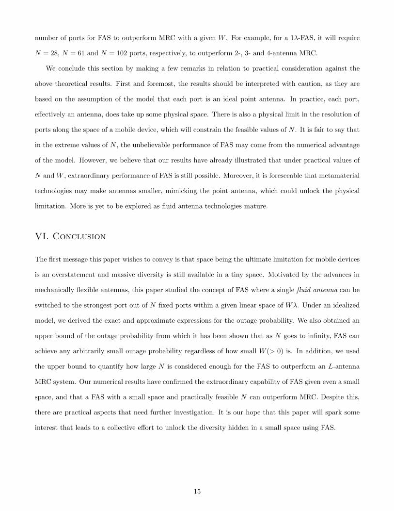
number of ports for FAS to outperform MRC with a given W . For example, for a 1λ-FAS, it will require
N = 28, N = 61 and N = 102 ports, respectively, to outperform 2-, 3- and 4-antenna MRC.
We conclude this section by making a few remarks in relation to practical consideration against the
above theoretical results. First and foremost, the results should be interpreted with caution, as they are
based on the assumption of the model that each port is an ideal point antenna. In practice, each port,
effectively an antenna, does take up some physical space. There is also a physical limit in the resolution of
ports along the space of a mobile device, which will constrain the feasible values of N . It is fair to say that
in the extreme values of N , the unbelievable performance of FAS may come from the numerical advantage
of the model. However, we believe that our results have already illustrated that under practical values of
N and W , extraordinary performance of FAS is still possible. Moreover, it is foreseeable that metamaterial
technologies may make antennas smaller, mimicking the point antenna, which could unlock the physical
limitation. More is yet to be explored as fluid antenna technologies mature.
VI. Conclusion
The first message this paper wishes to convey is that space being the ultimate limitation for mobile devices
is an overstatement and massive diversity is still available in a tiny space. Motivated by the advances in
mechanically flexible antennas, this paper studied the concept of FAS where a single fluid antenna can be
switched to the strongest port out of N fixed ports within a given linear space of Wλ. Under an idealized
model, we derived the exact and approximate expressions for the outage probability. We also obtained an
upper bound of the outage probability from which it has been shown that as N goes to infinity, FAS can
achieve any arbitrarily small outage probability regardless of how small W (> 0) is. In addition, we used
the upper bound to quantify how large N is considered enough for the FAS to outperform an L-antenna
MRC system. Our numerical results have confirmed the extraordinary capability of FAS given even a small
space, and that a FAS with a small space and practically feasible N can outperform MRC. Despite this,
there are practical aspects that need further investigation. It is our hope that this paper will spark some
interest that leads to a collective effort to unlock the diversity hidden in a small space using FAS.
15

V. Appendices
A. Derivation of p|g1|,|g2|,...,|gN |(r1, r2, . . . , rN)
Conditioned on x0, y0, |g2| is Rician distributed and therefore, we have
p|g2||x0,y0(r2|x0, y0) =
2r2
σ2(1− µ22)e− r
22+µ2
2(x20+y2
0)
σ2(1−µ22) I0
(σµ2
√x2
0 + y20r2
σ2
2 (1− µ22)
), for r2 ≥ 0. (30)
Given x0, y0, |g2|, |g3|, . . . , |gN | are all independent and we can obtain
p|g2|,...,|gN |||g1|(r2, . . . , rN |r1) =N∏k=2
2rkσ2(1− µ2
k)e− r2k+µ2
kr21
σ2(1−µ2k
) I0
(σµkr1r2
σ2
2 (1− µ2k)
), (31)
where r1 =√x2
0 + y20. With the pdf of |g1| given by (4), p|g2|,...,|gN |||g1|(r2, . . . , rN |r1)p|g1|(r1) gives the
desired result (11) which completes the proof.
B. Derivation of F|g1|,|g2|,...,|gN |(r1, r2, . . . , rN)
The joint pdf of |g1|, |g2|, . . . , |gN | can be obtained by
F|g1|,|g2|,...,|gN |(r1, r2, . . . , rN ) =
∫ r1
0· · ·∫ rN
0p|g1|,|g2|,...,|gN |(t1, t2, . . . , tN )dt1 · · · dtN . (32)
Substituting the result in (11) into the above, we get
F|g1|,|g2|,...,|gN |(r1, r2, . . . , rN ) =
∫ r1
0
2t1σ2e−
t21σ2
[N∏k=2
∫ rk
0
2tkσ2(1− µ2
k)e− t2k+µ2
kt21
σ2(1−µ2k
) I0
(2µkt1tk
σ2(1− µ2k)
)dtk
]dt1.
(33)
The integral inside the product operator appears to be an integration over the pdf of a Rician random
variable, which therefore gives
F|g1|,|g2|,...,|gN |(r1, r2, . . . , rN ) =
∫ r1
0
2t1σ2e−
t21σ2
N∏k=2
[1−Q1
(√2µ2
k
σ2(1− µ2k)t1,
√2
σ2(1− µ2k)rk
)]dt1. (34)
Now, changing the variable for the integration using t1 =r21σ2 obtains the final result (13).
16

C. Derivation of the Joint cdf when N = 2
To obtain the result, the following lemma is useful.
Lemma 3 It is known that
∫ c
0e−tQ1(a
√t, b)dt = e
− b2
a2+2Q1
(√c(a2 + 2),
ab√a2 + 2
)− e−cQ1(a
√c, b). (35)
Proof: The result can be directly obtained from [26, (B.19)] by simple changes of variables. �
Substituting N = 2 in (13), we get
F|g1|,|g2|(r1, r2) =
∫ r21σ2
0e−t
[1−Q1
(√2µ2
2
1− µ22
√t,
√2
σ2(1− µ22)rk
)]dt
= 1− e−r21σ2 −
∫ r21σ2
0e−tQ1
(√2µ2
2
1− µ22
√t,
√2
σ2(1− µ22)rk
)dt. (36)
Using (35) in Lemma 3 on the last term of the above by substituting a =
√2µ2
2
1−µ22, b =
√2
σ2(1−µ22)rk and
c =r21σ2 , we obtain the desired result, and complete the proof.
D. Derivation of the Approximate Outage Probability Expression
Note that 0 ≤ Q1(α, β) ≤ 1 and therefore we can approximate∏k(1−Q1(·, ·)) ≈ 1−
∑kQ1(·, ·) so that
pout(γth) ≈∫ γth
Γ
0e−t
[1−
N∑k=2
Q1
(√2µ2
k
1− µ2k
√t,
√2
1− µ2k
√γth
Γ
)]dt
= 1− e−γthΓ −
N∑k=2
∫ γthΓ
0e−tQ1
(√2µ2
k
1− µ2k
√t,
√2
1− µ2k
√γth
Γ
)dt. (37)
Using (35) in Lemma 3 by setting a =
√2µ2k
1−µ2k, b =
√2
1−µ2k
√γthΓ and c = γth
Γ for the integral inside the
summation achieves the approximate expression for the outage probability.
E. Tightness Analysis for (22)
Before we analyze (22), the following lemmas are useful.
Lemma 4 For 0 ≤ α ≤ β, Q1(α, β) can be upper-bounded by
17

Q1(α, β) <1√
1 + 2αβ
(β
β − α
). (38)
Proof: According to [27], for 0 ≤ α ≤ β, we have
Q1(α, β) ≤ I0(αβ)
eαβ
[e−
(β−α)2
2 + α
√π
2erfc
(β − α√
2
)], (39)
where erfc(·) denotes the complementary error function. Then we apply the upper bounds that erfc(x) ≤
e−x2
√πx
[28] and I0(x) < ex√1+2x
[29, (3.1)] into (39), giving
Q1(α, β) <1√
1 + 2αβ
(β
β − α
)e−
(β−α)2
2 <1√
1 + 2αβ
(β
β − α
), (40)
which reaches the desired result in (38). �
Lemma 5 Given 0 ≤ µ < 1 and X0 >√
1−µ2
2 , define the function f(x) : [0, X0]→ R,
f(x) =X0
(X0 − µx)
√1 +
(4µX0
1−µ2
)x
> 0, for x ∈ [0, X0]. (41)
Then f(x) is a decreasing function as x increases from 0 and may gradually become an increasing function
at some point but once it is increasing, it will continue to increase as x increases. As a result, the maximum
of f(x) appears at either x = 0 or x = X0. Also, f(0) = 1, f(X0) = 1
(1−µ)
√1+
4µX20
1−µ2
, and
∂f(x)
∂x
∣∣∣∣x=0
= − µ
1− µ2
(2X0 −
1− µ2
X0
). (42)
Proof: We first obtain the derivative of f(x) as
∂f(x)
∂x= −
µX0
[2X2
0 − 6µX0x− (1− µ2)]
(1− µ2)(X0 − µx)2(
1−µ2+4µX0x1−µ2
) 32
= −(+ve)
[2X2
0 − 6µX0x− (1− µ2)]
(+ve)(+ve)(+ve). (43)
Thus, the polarity of ∂f(x)∂x is decided by h(x) = 2X2
0 − (1−µ2)− 6µX0x. At x = 0, h(0) = 2X20 − (1−µ2)
and if X0 >√
1−µ2
2 , then h(0) > 0 and ∂f(x)∂x
∣∣∣x=0
< 0, which shows that f(x) is decreasing from x = 0.
In addition, h(x) is a decreasing function of x, meaning that if x is large enough, then h(x) may become
18

negative, making ∂f(x)∂x positive, and hence f(x) increasing afterwards. Because of how the value of f(x)
changes over x, the maximum must appear at one of the endpoints of the interval [0, X0]. Finally, the
values of f(0), f(X0), and ∂f(x)∂x
∣∣∣x=0
can be easily obtained from (41) and (43). �
Now, we are ready to study the tightness of the approximation (22). The approximation is based on∏k(1−Q1(αk, βk)) ≈ 1−
∑kQ1(αk, βk) which is accurate if Q1(αk, βk) is small. In the outage probability
computation, αk =
√2µ2k
1−µ2k
√t for 0 ≤ t ≤
√γthΓ and βk =
√2
1−µ2k
√γthΓ and hence, αk ≤ βk, we can use the
upper bound (38) in Lemma 4 on Q1(αk, βk) to yield
Q1(αk, βk) <
√γthΓ(√
γthΓ − µk
√t)√
1 +4µk
√γthΓ
1−µ2k
√t
, (44)
where the right-hand-side is recognized as f(x) in (41) with x =√t and X0 =
√γthΓ . The upper bound
of our interest in (44) concerns t ∈ (0, γthΓ ) (i.e., x ∈ (0, X0)) in the integration for computing the outage
probability (15). Using Lemma 5, the slope of the upper bound of Q1(αk, βk) at t = 0 is given by
∂f(√t)
∂√t
∣∣∣∣t=0
= − µk1− µ2
k
2
√γth
Γ−
1− µ2k√
γthΓ
, (45)
which will be negative and of a very large magnitude if either√
γthΓ is large or µk is close to one. If this
happens, the upper bound will stay near one only over an insignificant interval of t for the integration. In
addition, the upper bound will fall very sharply, and even if it increases again as t increases, the upper
bound will be limited by
f(X0) =1
(1− µk)√
1 +(
4µk1−µ2
k
)γthΓ
, (46)
which will be small if√
γthΓ is large enough. In summary, if
√γthΓ and/or {µk} are large enough, then the
upper bound (and hence Q1(αk, βk)) will be small over a significant interval of t for the integration (15)
and as a consequence, the approximation will be tight, which completes the proof.
19

F. Derivation of the Upper Bound, pUBout(γth)
To derive the upper bound, pUBout(γth), it suffices to obtain a lower bound for ∆pout(γth) because according
to Theorem 6, pNout(γth) = pN−1out (γth)−∆pout(γth) where the superscript n specifies the outage probability
for an n-port FAS. To proceed, the following lemma is useful.
Lemma 6 For 0 < α < β and large β, we have the following lower bound for Q1(α, β):
Q1(α, β) & %
√β
αe−
κ2
(β−α)2, (47)
where κ is any positive constant greater than one, and % , e1
π(κ−1)+2
2κ
√(κ−1)(π(κ−1)+2)
π .
Proof: For large β, we have Q1(α, β) ≈√
βαQ(β − α) [26, (A.4)] in which Q(x) = 1√
2π
∫∞x e−
t2
2 dt is
the Gaussian Q-function. Then applying the lower bound in [30, Theorem 2.1] gives the bound. �
Using Lemma 6, for 0 < t < γthΓ and large |µN |, we get
Q1
(√2µ2
N
1− µ2N
√t,
√2
1− µ2N
√γth
Γ
)&
%(γth
Γ
)0.25
t0.25√|µN |
e− κ
1−µ2N
(√γthΓ−µN
√t
)2
(a)>
%√|µN |
e− κ
1−µ2N
( γthΓ ), (48)
where (a) is obtained by choosing t = γthΓ in the denominator and t = 0 for the exponential function. As
a consequence, we can get a lower bound for ∆pout(γth) by
∆pout(γth) >
∫ γthΓ
0e−t
(%√|µN |
e− κ
1−µ2N
( γthΓ ))N−1∏k=2
[1−Q1
(√2µ2
k
1− µ2k
√t,
√2
1− µ2k
√γth
Γ
)]dt
= pN−1out (γth)× %√
|µN |e− κ
1−µ2N
( γthΓ ), (49)
20

which then gives
pNout(γth) < pN−1out (γth)
(1− %√
|µN |e− κ
1−µ2N
( γthΓ ))
< pN−2out (γth)
(1− %√
|µN−1|e− κ
1−µ2N−1
( γthΓ ))(
1− %√|µN |
e− κ
1−µ2N
( γthΓ ))
...
< p1out(γth)
N∏k=2
(1− %√
|µk|e− κ
1−µ2k( γth
Γ ))
=(
1− e−γthΓ
) N∏k=2
(1− %√
|µk|e− κ
1−µ2k( γth
Γ )), (50)
which is the desired result and completes the proof.
G. The Minimum Dimension of Fluid Antenna, W
Corollary 7 obtains the minimum required dimension d∗ to get the needed autocorrelation µ∗ so that FAS
outperforms MRC based on the upper bound of outage probability (24) for a fancy system where all the
autocorrelation parameters are the same. Now, imagine, if we have a FAS in which half of the ports, N2 ,
have dk < d∗ but another half have dk > d∗, then this FAS will have better outage probability performance
than an N2 -port FAS with µk = µ∗. As such, using the performance of the N
2 -port FAS with µk = µ∗ ∀k
as the worst-case performance for the N -port FAS with general {µk}, we can provide a sufficient condition
for the required dimension, Wλ, from the result of Corollary 7.
References
[1] H. Viswanathan, and M. Weldon, “The past, present, and future of mobile communications,” Bell Labs Tech. J., vol. 19,
pp. 8–21, Aug. 2014.
[2] A. J. Paulraj, and T. Kailath, “Increasing capacity in wireless broadcast systems using distributed transmission/directional
reception (DTDR),” US Patent 5,345,599A, granted 1994.
[3] G. J. Foschini, and M. J. Gans, “On limits of wireless communications in a fading environment when using multiple
antennas,” Wireless Pers. Commun., vol. 6, no. 3, pp. 311–335, Mar. 1998.
[4] V. Tarokh, N. Seshadri, and A. R. Calderbank, “Space-time codes for high data rate wireless communication: Performance
criterion and code construction,” IEEE Trans. Inform. Theory, vol. 44, no. 2, pp. 744-765, Mar. 1998.
[5] S. M. Alamouti, “A simple transmit diversity technique for wireless communications,” IEEE J. Select. Areas Commun.,
vol. 16, no. 8, pp. 1451–1458, Oct. 1998.
[6] L. Zheng, and D. N. C. Tse, “Diversity and multiplexing: A fundamental tradeoff in multiple-antenna channels,” IEEE
Trans. Inform. Theory, vol. 49, no. 5, pp. 1073–1096, May 2003.
[7] S. Vishwanath, N. Jindal, and A. Goldsmith, “Duality, achievable rates, and sum-rate capacity of Gaussian MIMO
broadcast channels,” IEEE Trans. Inform. Theory, vol. 49, no. 10, pp. 2658–2668, Oct. 2003.
[8] Q. H. Spencer, A. L. Swindlehurst, and M. Haardt, “Zero-forcing methods for downlink spatial multiplexing in multiuser
MIMO channels,” IEEE Trans. Signal Proc., vol. 52, no. 2, pp. 461–471, Feb. 2004.
21

[9] H. Q. Ngo, E. G. Larsson, and T. L. Marzetta, “Energy and spectral efficiency of very large multiuser MIMO systems,”
IEEE Trans. Commun., vol. 61, no. 4, pp. 1436–1449, Apr. 2013.
[10] E. G. Larsson, O. Edfors, F. Tufvesson, and T. L. Marzetta, “Massive MIMO for next generation wireless systems,” IEEE
Commun. Mag., vol. 52, no. 2, pp. 186–195, Feb. 2014.
[11] G. L. Stuber, Principles of Mobile Communication, Second Edition, Kluwer Academic Publishers, 2002.
[12] R. L. Haupt, and M. Lanagan, “Reconfigurable antennas,” IEEE Antennas and Propag. Mag., vol. 55, no. 1, pp. 49–61,
Feb. 2013.
[13] G. J. Hayes, J.-H. So, A. Qusba, M. D. Dickey, and G. Lazzi, “Flexible liquid metal alloy (EGaIn) microstrip patch
antenna,” IEEE Trans. Antennas Propag., vol. 60, no. 5, pp. 2151–2156, May 2012.
[14] A. M. Morishita, C. K. Y. Kitamura, A. T. Ohta, and W. A. Shiroma, “A liquid-metal monopole array with tunable
frequency, gain, and beam steering,” IEEE Antennas Wireless Propag. Lett., vol. 12, pp. 1388–1391, 2013.
[15] A. P. Saghati, J. Batra, J. Kameoka, and K. Entesari, “A microfluidically-tuned dual-band slot antenna,” in Proc. IEEE
Antennas Propag. Soc. Int. Symp. (APSURSI), pp. 1244–1245, 6-11 Jul. 2014, Memphis, TN, USA.
[16] A. Dey, R. Guldiken, and G. Mumcu, “Microfluidically reconfigured wideband frequency-tunable liquid-metal monopole
antenna,” IEEE Trans. Antennas Propag., vol. 64, no. 6, pp. 2572–2576, Jun. 2016.
[17] C. Borda-Fortuny, K.-F. Tong, A. Al-Armaghany, and K. K. Wong, “A low-cost fluid switch for frequency-reconfigurable
Vivaldi antenna,” IEEE Antennas Wireless Propag. Lett., vol. 16, pp. 3151–3154, 2017.
[18] C. Borda-Fortuny, K. F. Tong, and K. Chetty, “Low-cost mechanism to reconfigure the operating frequency band of a
Vivaldi antenna for cognitive radio and spectrum monitoring applications,” IET Microwaves, Antennas & Propag., vol.
12, no. 5, pp. 779–782, 2018.
[19] A. Singh, I. Goode, and C. E. Saavedra, “A multistate frequency reconfigurable monopole antenna using fluidic channels,”
IEEE Antennas Wireless Propag. Lett., vol. 18, no. 5, pp. 856–860, May 2019.
[20] C. Borda-Fortuny, L. Cai, K. F. Tong, and K. K. Wong, “Low-cost 3D-printed coupling-fed frequency agile fluidic
monopole antenna system,” IEEE Access, pp. 95058–95064, Jul. 2019.
[21] K. N. Paracha, A. D. Butt, A. S. Alghamdi, S. A. Babale, and P. J. Soh, “Liquid metal antennas: Materials, fabrication
and applications,” Sensors 2020, 20, 177.
[22] S. Song, and R. D. Murch, “An efficient approach for optimizing frequency reconfigurable pixel antennas using genetic
algorithms,” IEEE Trans. Antennas Propag., vol. 62, no. 2, pp. 609–620, Feb. 2014.
[23] N. Convery, and N. Gadegaard, “30 years of microfluidics,” Micro and Nano Engineering, vol. 2, pp. 76–91, Mar. 2019.
[24] O. C. Ugweje, and V. Aalo, “Performance of selection diversity system in correlated Nakagami fading,” in Proc. IEEE
Veh. Technol. Conf. (VTC), pp. 1488–1492, 4-7 May 1997, Phoenix, AZ, USA.
[25] L. Yang, and M.-S. Alouini, “An exact analysis of the impact of fading correlation on the average level crossing rate and
average outage duration of selection combining,” in Proc. IEEE Veh. Technol. Conf. (VTC-Spring), pp. 241–245, 22-25
Apr. 2003, Jeju, South Korea.
[26] M. K. Simon, Probability Distributions Involving Gaussian Random Variables: A Handbook for Engineers and Scientists,
Springer, Boston, MA, 2002.
[27] G. E. Corazza, and G. Ferrari, “New bounds for the Marcum Q-function,” IEEE Trans. Inform. Theory, vol. 48, pp.
3003–3008, Nov. 2002.
[28] F. R. Kschischang, The complementary error function, Available [Online]: https://www.comm.utoronto.ca/frank/notes/erfc.pdf.
[29] Z.-H. Yang, and Y.-M. Chu, “On approximating the modified Bessel function of the first kind and Toader-Qi mean,” J.
Inequalities and Appl., vol. 40, 2016.
[30] F. D. Cote, I. N. Psaromiligkos, and W. J. Gross, “A Chernoff-type lower bound for the Gaussian Q-function,” [Online].
Available: https://arxiv.org/abs/1202.6483.
22

(a) A typical received signal across a space of 2λ
(b) Comparison for a 100-port FAS with 2λ space and MRC at 5GHz at v = 30km/h
Figure 1: Examples for the fading envelopes.
23

Figure 2: A possible architecture for a FAS.
Figure 3: Outage probability against N for the FAS.
24

Figure 4: Outage probability approximations and bounds for the FAS when γthΓ = 0dB.
Figure 5: The required size of the FAS based on (29) for outperforming the respective MRC system whenγthΓ = 0dB. For example, ‘FAS>2-antenna MRC’ means that FAS outperforms 2-antenna MRC.
25