fluctuating loads notes

Shigley’s Mechanical Engineering Design, 9th Ed. Class Notes by: Dr. Ala Hijazi

CH 6 of 19

CH 6: Fatigue Failure Resulting from Variable Loading

Some machine elements are subjected to static loads and for such elements static failure theories are used to predict failure (yielding or fracture). However, most machine elements are subjected to varying or fluctuating stresses (due to the movement) such as shafts, gears, bearings, cams & followers,etc.

Fluctuating stresses (repeated over long period of time) will cause a part to fail (fracture) at a stress level much smaller than the ultimate strength (or even the yield strength in some casses).

Unlike static loading where failure usualy can be detected before it happens (due to the large deflections associated with plastic deformation), fatigue failures are usualy sudden and therefore dangerous.

Fatigue failure is somehow similar to brittle fracture where the fracture surfaces are prependicular to the load axis.

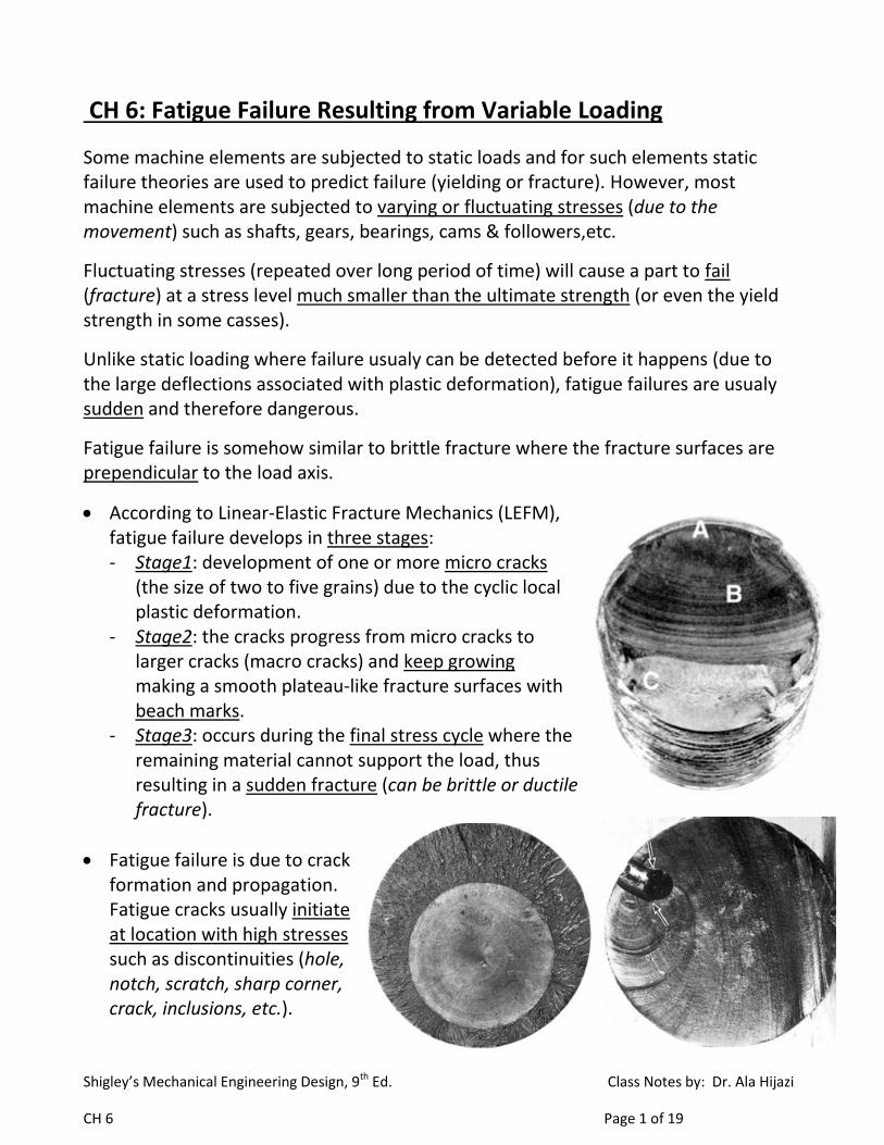
According to Linear-Elastic Fracture Mechanics (LEFM), fatigue failure develops in three stages: - Stage1: development of one or more micro cracks

(the size of two to five grains) due to the cyclic local plastic deformation.

- Stage2: the cracks progress from micro cracks to larger cracks (macro cracks) and keep growing making a smooth plateau-like fracture surfaces with beach marks.

- Stage3: occurs during the final stress cycle where the remaining material cannot support the load, thus resulting in a sudden fracture (can be brittle or ductile fracture).

Fatigue failure is due to crack formation and propagation. Fatigue cracks usually initiate at location with high stresses such as discontinuities (hole, notch, scratch, sharp corner, crack, inclusions, etc.).


CH 6 of 19

Fatigue cracks can also initiate at surfaces having rough surface finish or due to the presence of tensile residual stresses. Thus all parts subjected to fatigue loading are heat treated and polished in order to increase the fatigue life.

Fatigue Life Methods

Fatigue failure is a much more complicated phenomenon than static failure where much complicating factors are involved. Also, testing materials for fatigue properties is more complicated and much more time consuming than static testing.

Fatigue life methods are aimed to determine the life (number of loading cycles) of an element until failure.

There are three major fatigue life methods where each is more accurate for some types of loading or for some materials. The three methods are: the stress-life method, the strain-life method, the linear-elastic fracture mechanics method.

The fatigue life is usually classified according to the number of loading cycles into: Low cycle fatigue (1≤N≤1000) and for this low number of cycles, designers

sometimes ignore fatigue effects and just use static failure analysis. High cycle fatigue (N>103):

Finite life: from 103 →106 cycles Infinite life: more than 106 cycles

The Strain-Life Method

This method relates the fatigue life to the amount of

plastic strain suffered by the part during the repeated

loading cycles.

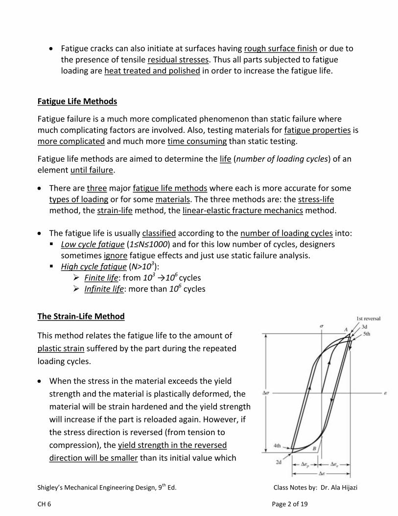
When the stress in the material exceeds the yield

strength and the material is plastically deformed, the

material will be strain hardened and the yield strength

will increase if the part is reloaded again. However, if

the stress direction is reversed (from tension to

compression), the yield strength in the reversed

direction will be smaller than its initial value which


CH 6 of 19

means that the material has been softened in the reverse loading direction. Each

time the stress is reversed, the yield strength in the other direction is decreased

and the material gets softer and undergoes more plastic deformation until fracture

occurs.

The strain-life method is applicable to Low-cycle fatigue.

The Linear Elastic Fracture Mechanics Method

This method assumes that a crack initiates in the material and it keeps growing until

failure occurs (the three stages described above).

The LEFM approach assumes that a small crack already exists in the material, and it

calculates the number of loading cycles required for the crack to grow to be large

enough to cause the remaining material to fracture completely.

This method is more applicable to High-cycle fatigue.

The Stress-Life Method

This method relates the fatigue life to the alternating stress level causing failure but it

does not give any explanation to why fatigue failure happens.

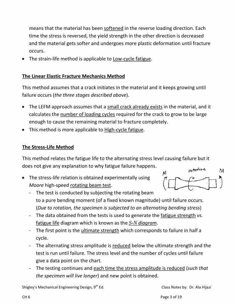
The stress-life relation is obtained experimentally using

Moore high-speed rotating beam test.

- The test is conducted by subjecting the rotating beam

to a pure bending moment (of a fixed known magnitude) until failure occurs.

(Due to rotation, the specimen is subjected to an alternating bending stress)

- The data obtained from the tests is used to generate the fatigue strength vs.

fatigue life diagram which is known as the S-N diagram.

- The first point is the ultimate strength which corresponds to failure in half a

cycle.

- The alternating stress amplitude is reduced below the ultimate strength and the

test is run until failure. The stress level and the number of cycles until failure

give a data point on the chart.

- The testing continues and each time the stress amplitude is reduced (such that

the specimen will live longer) and new point is obtained.


CH 6 of 19

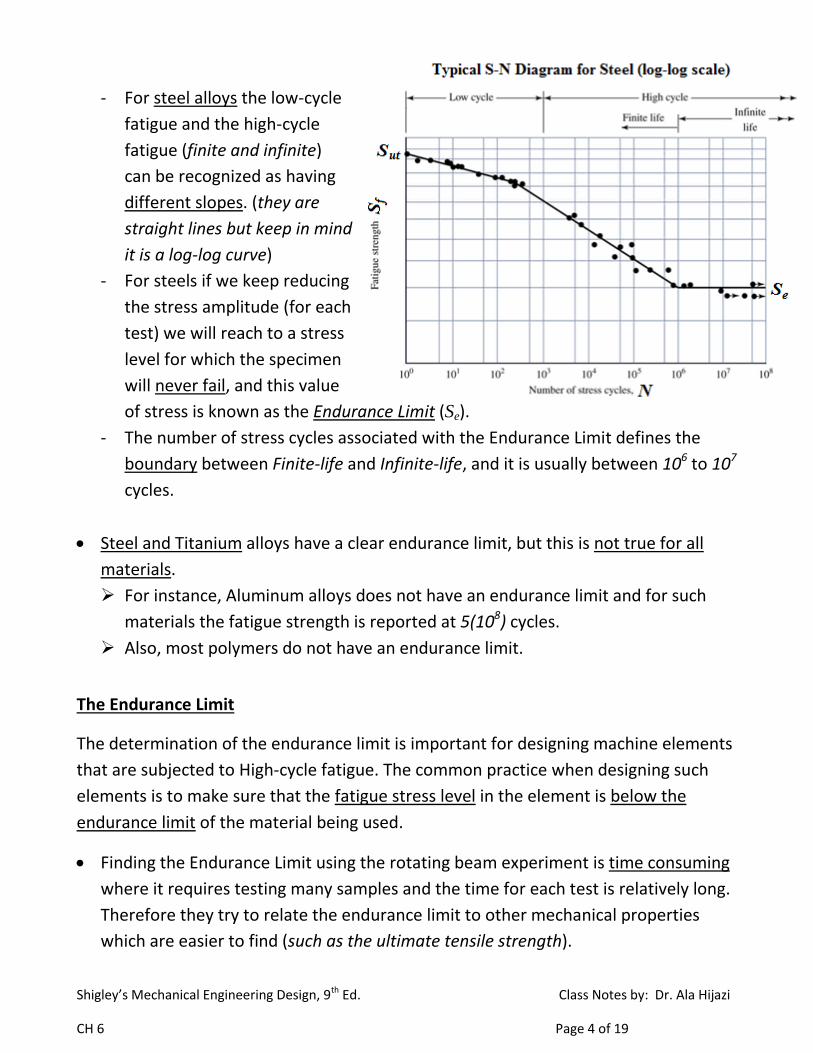
- For steel alloys the low-cycle

fatigue and the high-cycle

fatigue (finite and infinite)

can be recognized as having

different slopes. (they are

straight lines but keep in mind

it is a log-log curve)

- For steels if we keep reducing

the stress amplitude (for each

test) we will reach to a stress

level for which the specimen

will never fail, and this value

of stress is known as the Endurance Limit (Se).

- The number of stress cycles associated with the Endurance Limit defines the

boundary between Finite-life and Infinite-life, and it is usually between 106 to 107

cycles.

Steel and Titanium alloys have a clear endurance limit, but this is not true for all

materials.

For instance, Aluminum alloys does not have an endurance limit and for such

materials the fatigue strength is reported at 5(108) cycles.

Also, most polymers do not have an endurance limit.

The Endurance Limit

The determination of the endurance limit is important for designing machine elements

that are subjected to High-cycle fatigue. The common practice when designing such

elements is to make sure that the fatigue stress level in the element is below the

endurance limit of the material being used.

Finding the Endurance Limit using the rotating beam experiment is time consuming

where it requires testing many samples and the time for each test is relatively long.

Therefore they try to relate the endurance limit to other mechanical properties

which are easier to find (such as the ultimate tensile strength).


CH 6 of 19

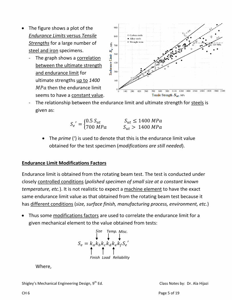
The figure shows a plot of the

Endurance Limits versus Tensile

Strengths for a large number of

steel and iron specimens.

- The graph shows a correlation

between the ultimate strength

and endurance limit for

ultimate strengths up to 1400

then the endurance limit

seems to have a constant value.

- The relationship between the endurance limit and ultimate strength for steels is

given as:

The prime (‘) is used to denote that this is the endurance limit value

obtained for the test specimen (modifications are still needed).

Endurance Limit Modifications Factors

Endurance limit is obtained from the rotating beam test. The test is conducted under

closely controlled conditions (polished specimen of small size at a constant known

temperature, etc.). It is not realistic to expect a machine element to have the exact

same endurance limit value as that obtained from the rotating beam test because it

has different conditions (size, surface finish, manufacturing process, environment, etc.)

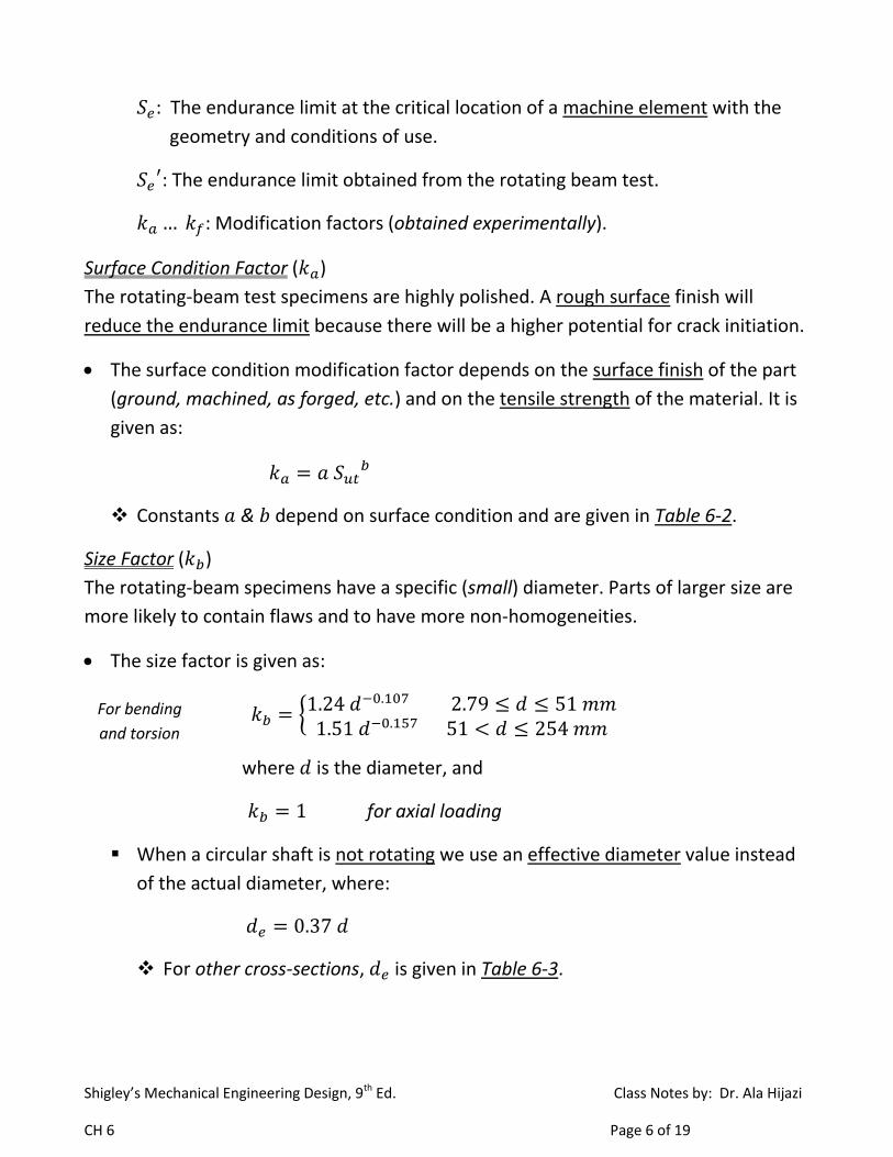
Thus some modifications factors are used to correlate the endurance limit for a

given mechanical element to the value obtained from tests:

Where,

Finish

Size

Reliability

Misc. Temp.

Load


CH 6 of 19

: The endurance limit at the critical location of a machine element with the

geometry and conditions of use.

: The endurance limit obtained from the rotating beam test.

: Modification factors (obtained experimentally).

Surface Condition Factor ( )

The rotating-beam test specimens are highly polished. A rough surface finish will

reduce the endurance limit because there will be a higher potential for crack initiation.

The surface condition modification factor depends on the surface finish of the part

(ground, machined, as forged, etc.) and on the tensile strength of the material. It is

given as:

Constants & depend on surface condition and are given in Table 6-2.

Size Factor ( )

The rotating-beam specimens have a specific (small) diameter. Parts of larger size are

more likely to contain flaws and to have more non-homogeneities.

The size factor is given as:

where is the diameter, and

for axial loading

When a circular shaft is not rotating we use an effective diameter value instead

of the actual diameter, where:

For other cross-sections, is given in Table 6-3.

For bending

and torsion


CH 6 of 19

Loading Factor ( )

The rotating-beam specimen is loaded in bending. Other types of loading will have a

different effect.

The load factor for the different types of loading is:

Temperature Factor ( ) When the operating temperature is below room temperature, the material becomes more brittle. When the temperature is high the yield strength decreases and the material becomes more ductile (and creep may occur).

For steels, the endurance limit slightly increases as temperature rises, then it starts to drop. Thus, the temperature factor is given as:

For

The same values calculated by the equation are also presented in Table 6-4

where:

Reliability Factor ( )

The endurance limit obtained from testing is usually reported at mean value (it has a

normal distribution with ).

For other values of reliability, is found from Table 6-5.

Miscellaneous-Effects Factor ( )

It is used to account for the reduction of endurance limit due to all other effects (such

as Residual stress, corrosion, cyclic frequency, metal spraying, etc.).

However, those effects are not fully characterized and usually not accounted for. Thus

we use ( ).


CH 6 of 19

Stress Concentration and Notch Sensitivity

Under fatigue loading conditions, crack initiation and growth usually starts in locations

having high stress concentrations (such as grooves, holes, etc.). The presence of stress

concentration reduces the fatigue life of an element (and the endurance limit) and it

must be considered in fatigue failure analysis.

However, due to the difference in ductility, the effect of stress concentration on

fatigue properties is not the same for different materials.

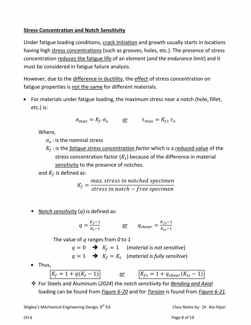
For materials under fatigue loading, the maximum stress near a notch (hole, fillet,

etc.) is:

or

Where,

: is the nominal stress

: is the fatigue stress concentration factor which is a reduced value of the

stress concentration factor ( ) because of the difference in material

sensitivity to the presence of notches.

and is defined as:

Notch sensitivity ( ) is defined as:

or

The value of ranges from 0 to 1

(material is not sensitive)

(material is fully sensitive)

Thus,

or

For Steels and Aluminum (2024) the notch sensitivity for Bending and Axial

loading can be found from Figure 6-20 and for Torsion is found from Figure 6-21.


CH 6 of 19

For cast iron, the notch sensitivity is very low from 0 to 0.2, but to be

conservative it is recommended to use

Heywood distinguished between different types of notches (hole, shoulder,

groove) and according to him, is found as:

Where, : radius

: is a constant that depends on the type of the notch.

For steels, for different types of notches is given in Table 6-15.

For simple loading, can be multiplied by the stress value, or the endurance limit

can be reduced by dividing it by . However, for combined loading each type of

stress has to be multiplied by its corresponding value.

Fatigue Strength

In some design applications the number of load cycles the element is subjected to is

limited (less than 106) and therefore there is no need to design for infinite life using the

endurance limit.

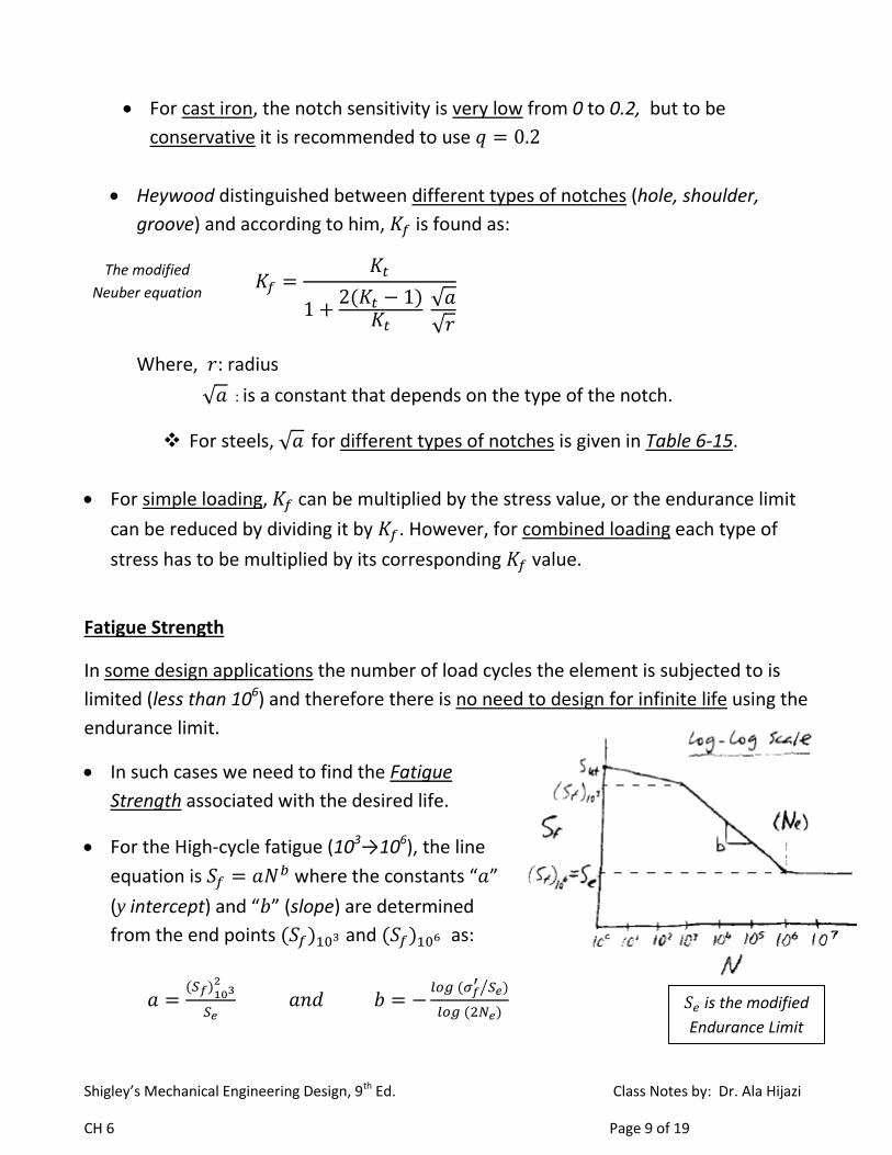
In such cases we need to find the Fatigue

Strength associated with the desired life.

For the High-cycle fatigue (103→106), the line

equation is where the constants “ ”

(y intercept) and “ ” (slope) are determined

from the end points and as:

The modified

Neuber equation

is the modified

Endurance Limit


CH 6 of 19

Where is the True Stress at Fracture and for steels with HB ≤ 500, it is

approximated as:

- can be related to as:

where is found as:

Using the above equations, the value of is found as a function

of (using ) and it is presented in graphical form in

Figure 6-18.

- If the value of ( ) is known, the constant can be directly found as:

and can be rewritten as:

- Thus for 103≤ ≤106 , the fatigue strength associated with a given life ( ) is:

and the fatigue life ( ) at a given fatigue stress ( ) is found as:

Studies show that for ductile materials, the Fatigue Stress Concentration Factor ( )

reduces for , however the conservative approach is to use as is.

Example: For a rotating-beam specimen made of 1050 CD steel, find:

fraction of

For values less than

490 MPa, use

to be conservative


CH 6 of 19

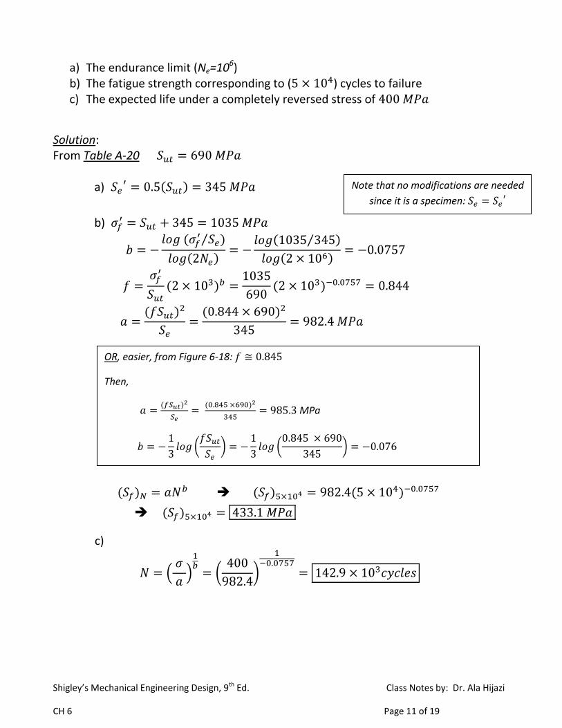
a) The endurance limit (Ne=106) b) The fatigue strength corresponding to ( ) cycles to failure c) The expected life under a completely reversed stress of

Solution: From Table A-20

a)

b)

c)

Note that no modifications are needed

since it is a specimen:

OR, easier, from Figure 6-18:

Then,

MPa


CH 6 of 19

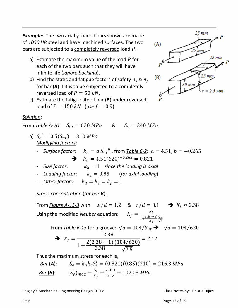
Example: The two axially loaded bars shown are made of 1050 HR steel and have machined surfaces. The two bars are subjected to a completely reversed load .

a) Estimate the maximum value of the load for each of the two bars such that they will have infinite life (ignore buckling).

b) Find the static and fatigue factors of safety &

for bar (B) if it is to be subjected to a completely reversed load of .

c) Estimate the fatigue life of bar (B) under reversed load of (use )

Solution:

From Table A-20 &

a)

Modifying factors:

- Surface factor: , from Table 6-2: ,

- Size factor: since the loading is axial

- Loading factor: (for axial loading)

- Other factors:

Stress concentration (for bar B):

From Figure A-13-3 with &

Using the modified Neuber equation:

From Table 6-15 for a groove:

Thus the maximum stress for each is,

Bar (A):

Bar (B):


CH 6 of 19

And the maximum load for each is,

Bar (A):

Bar (B):

Note that the maximum load for bar (B) is smaller than that of bar (A)

because of the notch.

b) Static factor of safety :

From Table A-20: Ductile material, thus stress concentration is

not applicable.

Fatigue factor of safety :

c) If we calculate the fatigue factor of safety with we will find it to be less than one and thus the bar will not have infinite life.

This gives more conservative results than dividing ( ) by , and using

as is.


CH 6 of 19

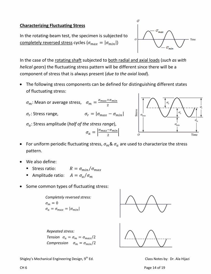
Characterizing Fluctuating Stress

In the rotating-beam test, the specimen is subjected to

completely reversed stress cycles ( )

In the case of the rotating shaft subjected to both radial and axial loads (such as with

helical gears) the fluctuating stress pattern will be different since there will be a

component of stress that is always present (due to the axial load).

The following stress components can be defined for distinguishing different states

of fluctuating stress:

: Mean or average stress,

: Stress range,

: Stress amplitude (half of the stress range),

For uniform periodic fluctuating stress, & are used to characterize the stress

pattern.

We also define:

Stress ratio:

Amplitude ratio:

Some common types of fluctuating stress:

Completely reversed stress:

Repeated stress:

Tension

Compression


CH 6 of 19

Fatigue Failure Criteria for Fluctuating Stress

When a machine element is subjected to completely reversed stress (zero mean,

) the endurance limit is obtained from the rotating-beam test (after applying

the necessary modifying factors).

However, when the mean (or midrange) is non-zero the situation is different and a

fatigue failure criteria is needed.

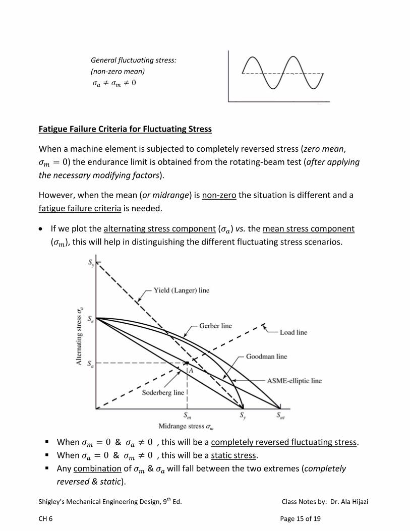
If we plot the alternating stress component ( ) vs. the mean stress component

( ), this will help in distinguishing the different fluctuating stress scenarios.

When & , this will be a completely reversed fluctuating stress.

When & , this will be a static stress.

Any combination of & will fall between the two extremes (completely

reversed & static).

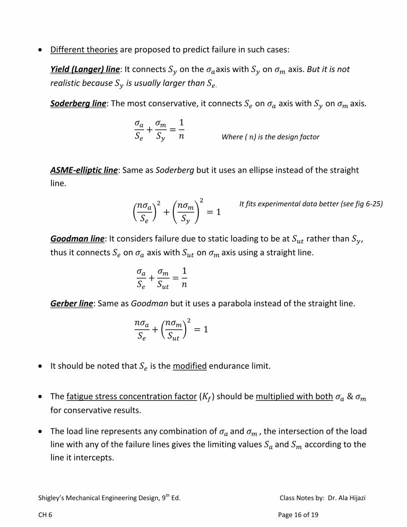
General fluctuating stress:

(non-zero mean)


CH 6 of 19

Different theories are proposed to predict failure in such cases:

Yield (Langer) line: It connects on the axis with on axis. But it is not

realistic because is usually larger than .

Soderberg line: The most conservative, it connects on axis with on axis.

ASME-elliptic line: Same as Soderberg but it uses an ellipse instead of the straight

line.

Goodman line: It considers failure due to static loading to be at rather than ,

thus it connects on axis with on axis using a straight line.

Gerber line: Same as Goodman but it uses a parabola instead of the straight line.

It should be noted that is the modified endurance limit.

The fatigue stress concentration factor ( ) should be multiplied with both &

for conservative results.

The load line represents any combination of and , the intersection of the load

line with any of the failure lines gives the limiting values and according to the

line it intercepts.

Where ( ) is the design factor

It fits experimental data better (see fig 6-25)


CH 6 of 19

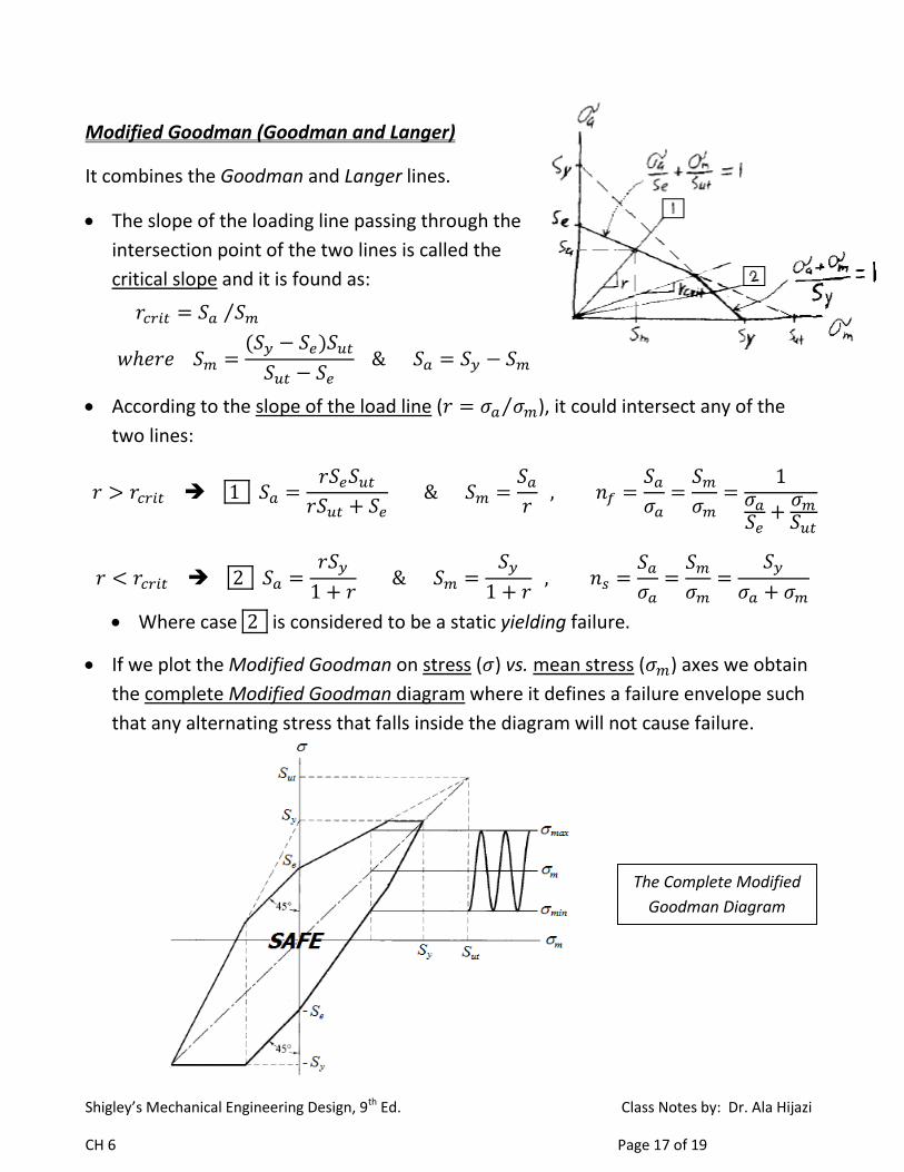
Modified Goodman (Goodman and Langer)

It combines the Goodman and Langer lines.

The slope of the loading line passing through the

intersection point of the two lines is called the

critical slope and it is found as:

According to the slope of the load line ( ), it could intersect any of the

two lines:

Where case is considered to be a static yielding failure.

If we plot the Modified Goodman on stress ( ) vs. mean stress ( ) axes we obtain

the complete Modified Goodman diagram where it defines a failure envelope such

that any alternating stress that falls inside the diagram will not cause failure.

The Complete Modified

Goodman Diagram


CH 6 of 19

Also, there are other modified criteria:

Gerber-Langer (see Table 6-7)

ASME-elliptic-Langer (see Table 6-8)

Example: A diameter bar has been machined from AISI-1045 CD bar. The bar

will be subjected to a fluctuating tensile load varying from to . Because of the

ends fillet radius, is to be used.

Find the critical mean and alternating stress values and the fatigue factor of safety according to the Modified Goodman fatigue criterion.

Solution:

From Table A-20

Modifying factors:

- Surface factor: (Table 6-2)

- Size factor: since the loading is axial

- Loading factor: (for axial loading)

- Other factors:

Fluctuating stress:

,

Applying to both components:


CH 6 of 19

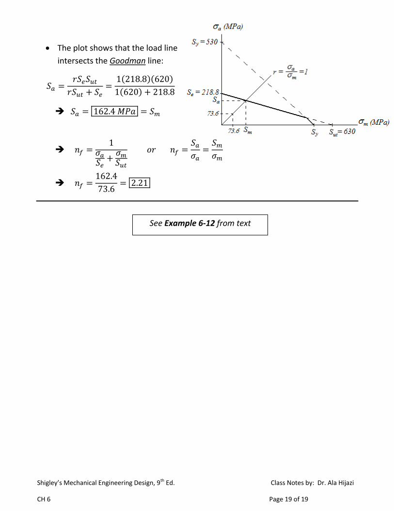
The plot shows that the load line

intersects the Goodman line:

See Example 6-12 from text