flow shop scheduling with peak power consumption constraints · flow shop scheduling with peak...
TRANSCRIPT

Flow Shop Scheduling with Peak Power Consumption Constraints
Kan Fang∗ Nelson A. Uhan† Fu Zhao‡ John W. Sutherland§
Abstract
We study scheduling as a means to address the increasing energy concerns in manufacturing
enterprises. In particular, we consider a flow shop scheduling problem with a restriction on peak
power consumption, in addition to the traditional time-based objectives. We investigate both
mathematical programming and combinatorial approaches to this scheduling problem, and test
our approaches with instances arising from the manufacturing of cast iron plates.
Keywords: scheduling; flow shop; energy; peak power consumption; integer programming;
combinatorial optimization
1 Introduction
Under the pressures of climate change, increasing energy costs, and growing energy security concerns,
manufacturing enterprises have become more and more interested in reducing their energy and power
consumption. Until recently, most efforts aimed at minimizing energy and power consumption in
manufacturing have been focused on developing machines and equipment that are more energy and
power efficient. However, several researchers have observed that in various manufacturing enterprises,
energy and power consumption can also be reduced through alternate operational strategies, such
as the smarter management and scheduling of machine start-up and machine idling (e.g. Dahmus
and Gutowski 2004; Gutowski et al. 2005; Drake et al. 2006). In this work, we explore the use of
scheduling as a means to reduce the energy and power consumption of manufacturing enterprises.
∗School of Industrial Engineering, Purdue University, West Lafayette, IN 47904, USA, e-mail: [email protected]†Corresponding author. Mathematics Department, United States Naval Academy, Annapolis, MD 21403, USA,
phone: +1 410-293-6713, fax: +1 410-293-4883, e-mail: [email protected]‡Division of Environmental and Ecological Engineering and School of Mechanical Engineering, Purdue University,
West Lafayette, IN 47904, USA, e-mail: [email protected]§Division of Environmental and Ecological Engineering and School of Mechanical Engineering, Purdue University,
West Lafayette, IN 47904, USA, e-mail: [email protected]
1
Research on using scheduling to reduce energy and power consumption in manufacturing is
rather sparse. One exception is the work by Mouzon et al. (2007), who proposed several dispatching
rules and a multi-objective mathematical programming formulation for scheduling jobs on a single
CNC machine in a way that minimizes energy consumption and total completion time. In addition,
Mouzon and Yildirim (2008) proposed a metaheuristic algorithm to minimize the total energy
consumption and total tardiness on a single machine. Fang et al. (2011) provided some preliminary
insights into the modeling and algorithmic challenges of shop scheduling problems with energy and
power criteria.
On the other hand, there is a considerable body of literature on scheduling computer processors
in a way that minimizes energy consumption. In these settings, the processors can be run at varying
speeds: reducing the speed of a processor lowers power consumption, but results in longer processing
time. This energy saving technique is called dynamic voltage scaling, or speed scaling, and was
originally studied by Yao et al. (1995). In most of the research on speed scaling, it is assumed
that the processor speed can be chosen arbitrarily from a continuous range and the associated
power consumption is an exponential function of the speed. One example of work done under this
assumption is that of Bansal et al. (2007), who studied the design and performance of speed scaling
algorithms for scheduling jobs with deadlines to address concerns with energy and temperature.
Other researchers have also considered the case where only a number of discrete speeds are available.
For example, Kwon and Kim (2005) proposed a voltage allocation technique for discrete supply
voltages to produce a preemptive task schedule that minimizes total energy consumption. Other
power functions have also been considered in the literature (e.g. Bansal et al. 2009). For more
pointers on the ever-growing literature on speed scaling, we refer the reader to the surveys by Irani
and Pruhs (2005) and Albers (2010).
In the speed scaling literature, it is typically assumed that each job needs to be processed on a
single processor or one of multiple parallel processors. This is to be expected, as this matches typical
computing environments. However, in a typical manufacturing environment, jobs often need to be
processed on multiple machines in some order; in other words, in some kind of job shop environment.
As a result, much of the work on speed scaling is not directly applicable to the problems faced by
manufacturing enterprises. In this work, we aim to begin to fill this gap. In particular, we consider
a permutation flow shop scheduling problem with objectives based on time and power. To the best
2

of our knowledge, our paper is one of the first in-depth studies of shop scheduling with both time
and power related criteria.
Most recent research assumes that reducing the average power consumption proportionately
decreases energy costs. However, peak power consumption – that is, the maximum power consumption
over all time instances – also plays a key role in the energy costs of electricity-intensive manufacturing
enterprises; for example, many energy providers use time-of-use (TOU) tariffs (e.g. Babu and Ashok
2008). Peak power consumption has also received some attention in the speed scaling literature,
since it affects the power supply and cooling technologies in the design of computer processors.
Several researchers have studied different approaches to reduce peak power consumption on a single
processor or parallel processors (e.g. Felter et al. 2005; Kontorinis et al. 2009; Cochran et al. 2011).
Due to the nature of energy costs in manufacturing environments, we consider the multi-objective
problem of minimizing the makespan and the peak power consumption in a permutation flow shop.
In particular, we search for Pareto optimal schedules, or schedules for which no other schedule has
both lower makespan and lower peak power consumption. In order to handle the bicriteria nature of
this problem, we fix an upper bound on the peak power consumption, and minimize the makespan
of the schedule. We consider the problem when speeds are discrete and when they are continuous.
In addition, we consider flow shops with both zero and unlimited intermediate storage between
machines. (In a flow shop with zero intermediate storage, a completed job cannot leave the current
machine until the the next machine is available.) For simplicity, in this paper, we refer to this
problem as the permutation flow shop scheduling problem with peak power consumption constraints,
or the PFSPP problem for short.
We consider both mathematical programming and combinatorial approaches to the PFSPP
problem. Unlike most classical scheduling problems, we need to be able to keep track of which jobs
are running concurrently at any time in order to take the peak power consumption into account.
This presents some interesting modeling and algorithmic challenges, and some of our results may be
of interest in other scheduling applications (e.g. Thornblad et al. 2010). For the case of discrete
speeds and unlimited intermediate storage, we propose two mixed integer programming formulations,
inspired by existing formulations for shop scheduling problems (Manne 1960; Lasserre and Queyranne
1992). In order to strengthen these formulations, we give valid inequalities that exploit the structure
of optimal schedules and the properties of concurrently running jobs. We also test the computational
3
performance of these two formulations and the effectiveness of these valid inequalities on a set of
instances based on the manufacture of cast iron plates with slots.
We also examine the PFSPP problem with two machines and zero intermediate storage. When
speeds are discrete, we show that this problem is equivalent to a special case of the asymmetric
traveling salesperson problem. On the other hand, when speeds are continuous, we assume that
power consumption is an exponential function of speed. In this case, we show that there exists
an optimal schedule in which the total peak power consumption at any time instant is equal
to exactly the fixed upper bound, and that this problem can be transformed to an equivalent
asymmetric traveling salesperson problem. Moreover, if the jobs have some special features, we
obtain combinatorial polynomial time algorithms for finding optimal schedules.
2 Mathematical description of the problem
As we mentioned in the introduction, we refer to the flow shop scheduling problem that we study in
this paper as the permutation flow shop problem with power consumption constraints (or the PFSPP
problem for short). An instance of the PFSPP problem consists of a set J = 1, 2, . . . , n of jobs
and a set M = 1, 2, . . . ,m of machines. Each job j on machine i has a work requirement pij ,
and must be processed nonpreemptively first on machine 1, then on machine 2, and so on. There
is a set of speeds S: a job j ∈ J processed on machine i ∈ M at speed s ∈ S has an associated
processing time pijs and power consumption qijs. In addition, we are given a threshold Qmax on the
total power consumption at any time instant of the schedule.
Assumption 2.1. We assume that when we process a job at a higher speed, its processing time
decreases, while its power consumption increases. That is, as s increases, pijs decreases and qijs
increases. In addition, we assume that the power consumption associated with processing a job on
a machine at a particular speed is constant from the job’s start time until but not including the
job’s completion time. Finally, we assume that mins∈Sqijs ≤ Qmax for all i ∈M and j ∈ J .
In this paper, we focus on minimizing the makespan Cmax, the completion time of the last
job on the last machine m. We define a feasible schedule as a schedule in which the total power
consumption at any time is no more than the given threshold Qmax. Then, depending on the type
of the speed set and flow shop environment, we define the following variants of the PFSPP problem.
4

Problem 2.2. The set of speeds set S = s1, s2, . . . , sd is discrete. The flow shop has unlimited
intermediate storage. Each job j ∈ J on machine i ∈ M has processing time pijs and power
consumption qijs when processed at speed s ∈ S. Find a feasible schedule that minimizes the
makespan Cmax.
Instead of giving an explicit equation for power as a function of speed, we assume that the
relationship between processing time, power consumption and speed can be arbitrary in Problem 2.2,
as long as it satisfies Assumption 2.1. Without loss of generality, we assume that s1 < s2 < · · · < sd.
We also consider a variant of Problem 2.2, in which the flow shop has two machines and zero
intermediate storage.
Problem 2.3. The set of speeds S = s1, s2, . . . , sd is discrete. The flow shop has two machines,
that is, M = 1, 2, and zero intermediate storage. Each job j ∈ J on machine i ∈ M has
processing time pijs and power consumption qijs when processed at speed s ∈ S. Find a feasible
solution that minimizes the makespan Cmax.
Unlike in Problems 2.2 and 2.3, it might be the case that each job can run at an arbitrary speed
within a given continuous range. It is typical to have power as an exponential function of speed (e.g.
Bouzid 2005; Mudge 2001). We consider the following two machine variant of the PFSPP problem
with zero intermediate storage.
Problem 2.4. The set of speeds S = [smin, smax] is continuous. The flow shop has two machines,
that is,M = 1, 2, and zero intermediate storage. Each job j processed on machine i at speed s ∈ S
has processing time pijs = pij/s and power consumption qijs = sα for some constant α > 1. Find a
feasible schedule that minimizes the makespan Cmax.
3 Discrete speeds and unlimited intermediate storage: mixed in-
teger programming formulations
A great deal of research has focused on solving the ordinary permutation flow shop scheduling
problem (without power consumption considerations) with integer programming approaches. These
efforts have primarily looked at two families of mixed integer programs. One is based on Manne’s
5

(1960) formulation that uses linear ordering variables and pairs of dichotomous constraints (called
the disjunctive constraints) to ensure one job is processed before another or vice versa. The other is
based on Wagner’s (1959) use of the classical assignment problem to assign jobs to positions on
machines. Researchers have investigated the computational performance of different mixed integer
programs for the oridnary permutation flow shop scheduling problem from these two families with
respect to various objectives (e.g. Stafford Jr. et al. 2005; Keha et al. 2009; Unlu and Mason 2010).
In this work, we propose two mixed integer programming formulations, inspired by the work
of Manne (1960) and Wagner (1959). In particular, we follow a variant of Wagner’s formulation
proposed by Lasserre and Queyranne (1992), which models the relationship between jobs and
their position in a permutation. We will compare the performance of these two mixed integer
programming formulations to discover some promising formulation paradigms that can subsequently
be applied to solve larger scheduling problems with peak power consumption constraints.
Unlike most ordinary flow shop scheduling problems, in the PFSPP problem, we need to keep
track of jobs that are running concurrently on machines at any time. For this reason, we cannot
directly apply the existing mixed integer programming formulations mentioned above. In order to
build upon these formulations, we use the following observation. Note that in the PFSPP problem,
each job must be processed nonpreemptively with exactly one speed s ∈ S on each machine. As a
result, when a job is started on a given machine, the power consumption of that machine will stay
the same until this job is finished. For any time instance t, let Jt be the set of jobs being processed
at t. Let CLt (SLt ) be the completion (start) time of the last job that is completed (started) before
time t. Let CRt (SRt ) be the completion (start) time of the first job that is completed (started)
after time t. Denote t1 = maxCLt , SLt and t2 = minCRt , SRt . Then for any time t′ within [t1, t2),
we have Jt′ = Jt, which implies that the total power consumption in the flow shop is a constant
between t1 and t2.
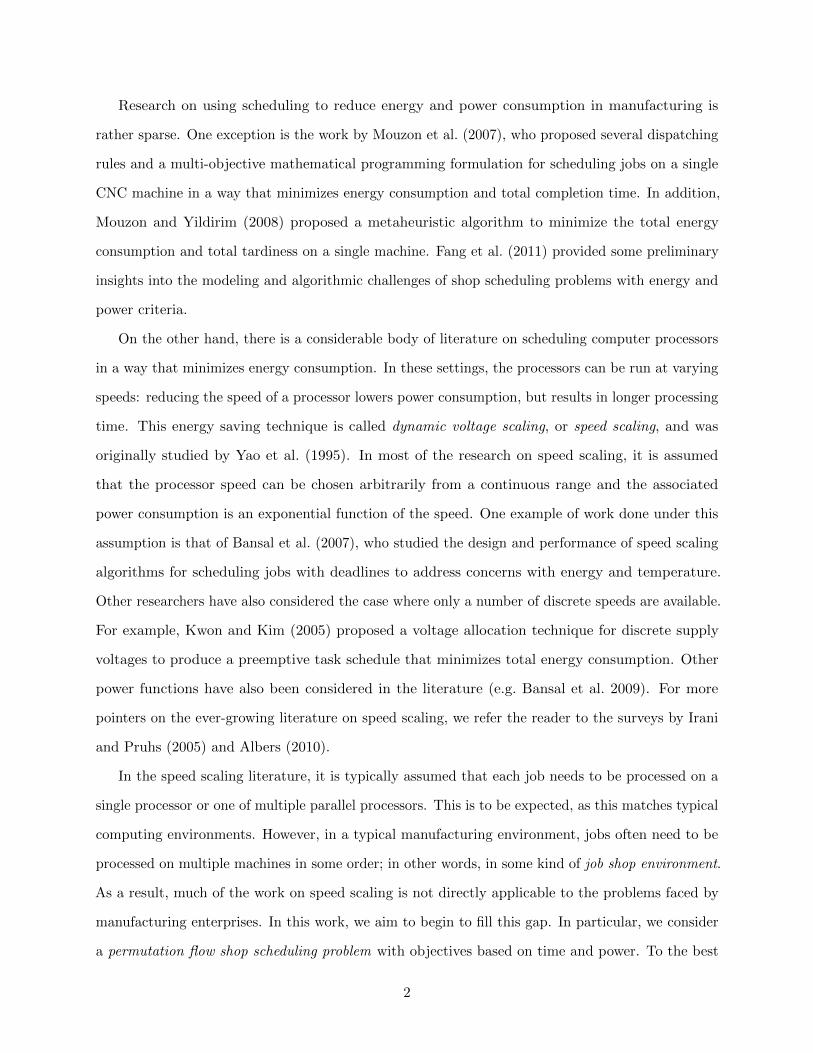
Example 3.1. Consider the following example that illustrates the above observation. At time t,
there are three jobs Jt = j, k, l that are processed concurrently (see Figure 1). SLt is the start
time of job k on machine g, CLt is the completion time of job r on machine i. In this example,
SLt < CLt , so we have t1 = CLt . Similarly, we have t2 = CRt , which is the completion time of job j
on machine f . Then within [t1, t2), the total power consumption in the flow shop is constant.
6
j
k
l
r o
tt1 t2
... ...
... ...
... ...
... ...
machine h
machine g
machine f
machine i
Figure 1: Gantt chart for Example 3.1.
Inspired by this observation, we propose mixed integer programs with binary variables that
keep track of jobs that are running concurrently on any two different machines only at job start
and completion times. First, we propose a mixed integer program in Section 3.1 inspired by Manne
(1960), which we will call the disjunctive formulation. In Section 3.2, we propose another mixed
integer program inspired by Lasserre and Queyranne (1992), which we will call the assignment and
positional formulation (or AP formulation for short).
3.1 Disjunctive formulation
In this section, we propose a mixed integer program inspired by Manne’s (1960) formulation. We
define the following decision variables:
• Cmax is the makespan of the schedule;
• Cij is the completion time of job j on machine i;
• Sij is the start time of job j on machine i;
• δjk is equal to 1 if job j precedes job k, and 0 otherwise;
• xijs is equal to 1 if job j is processed on machine i with speed s, and 0 otherwise;
• uhkij is equal to 1 if the start time of job k on machine h is less than or equal to the start
time of job j on machine i (in other words, Shk ≤ Sij), and 0 otherwise;
• vhkij is equal to 1 if the completion time of job k on machine h is greater than the start time
of job j on machine i (in other words, Chk > Sij), and 0 otherwise;
7
• yhkij is equal to 1 if the start time of job j on machine i occurs during the processing of job k
on machine h (in other words, Shk ≤ Sij < Chk), and 0 otherwise;
• zhksij is equal to 1 if job k is processed on machine h with speed s, and starts while job j is
running on machine i (in other words, if xhks = 1 and yhkij = 1), and 0 otherwise.
We call the binary decision variables u, v, y and z the concurrent job variables. Let M be an
upper bound on the makespan of an optimal schedule. For simplicity, we let M =∑
i∈M∑
j∈J pij1.
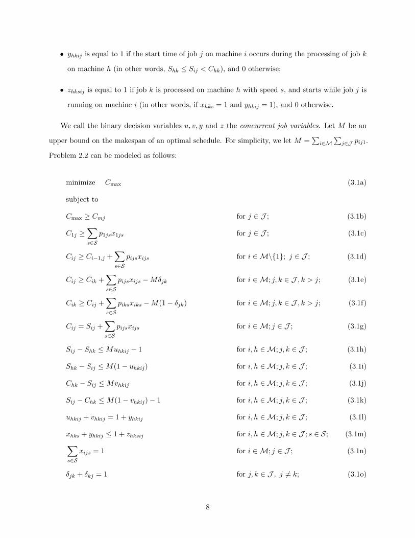
Problem 2.2 can be modeled as follows:
minimize Cmax (3.1a)
subject to
Cmax ≥ Cmj for j ∈ J ; (3.1b)
C1j ≥∑s∈S
p1jsx1js for j ∈ J ; (3.1c)
Cij ≥ Ci−1,j +∑s∈S
pijsxijs for i ∈M\1; j ∈ J ; (3.1d)
Cij ≥ Cik +∑s∈S
pijsxijs −Mδjk for i ∈M; j, k ∈ J , k > j; (3.1e)
Cik ≥ Cij +∑s∈S
piksxiks −M(1− δjk) for i ∈M; j, k ∈ J , k > j; (3.1f)
Cij = Sij +∑s∈S
pijsxijs for i ∈M; j ∈ J ; (3.1g)
Sij − Shk ≤Muhkij − 1 for i, h ∈M; j, k ∈ J ; (3.1h)
Shk − Sij ≤M(1− uhkij) for i, h ∈M; j, k ∈ J ; (3.1i)
Chk − Sij ≤Mvhkij for i, h ∈M; j, k ∈ J ; (3.1j)
Sij − Chk ≤M(1− vhkij)− 1 for i, h ∈M; j, k ∈ J ; (3.1k)
uhkij + vhkij = 1 + yhkij for i, h ∈M; j, k ∈ J ; (3.1l)
xhks + yhkij ≤ 1 + zhksij for i, h ∈M; j, k ∈ J ; s ∈ S; (3.1m)∑s∈S
xijs = 1 for i ∈M; j ∈ J ; (3.1n)
δjk + δkj = 1 for j, k ∈ J , j 6= k; (3.1o)
8
δjk + δkl + δlj ≤ 2 for j, k, l ∈ J , j 6= k 6= l; (3.1p)∑s∈S
qijsxijs +∑
h∈M,h6=i
∑k∈J
∑s∈S
qhkszhksij ≤ Qmax for i ∈M; j ∈ J ; (3.1q)
xijs, δjk, uhkij , vhkij , yhkij , zhksij ∈ 0, 1 for i, h ∈M; j, k ∈ J ; s ∈ S. (3.1r)
The objective (3.1a) and the constraints (3.1b) ensure that the makespan is equal to the completion
time of the last job processed on machine m. Constraints (3.1c)-(3.1f) ensure that the completion
times are consistent with a flow shop. In particular, constraints (3.1e)-(3.1f) are the disjunctive
constraints between any two jobs j and k: they ensure that job j is processed before job k or vice
versa. Constraints (3.1g) ensure that jobs are processed nonpreemptively. Constraints (3.1h)-(3.1m)
ensure that the concurrent job variables u, v, y and z take their intended values. Constraints (3.1n)
indicate that each job can be processed on any given machine with exactly one speed. Constraints
(3.1o)-(3.1p) ensure that the jobs are processed in the same order on every machine. Finally,
constraints (3.1q) ensure that at any time, the total power consumption across machines does not
exceed the threshold Qmax.
3.2 Assignment and positional formulation
Next, we give another formulation of our problem, inspired by the formulation proposed by
Lasserre and Queyranne (1992), which uses binary variables to directly assign jobs to positions in
a permutation. A variant of this formulation was proposed in Fang et al. (2011). We define the
following decision variables:
• Cmax is the makespan of the schedule;
• Cij is the completion time of the jth job processed on machine i (note that “jth job” refers
to the jth position, not job j);
• Sij is the start time of the jth job processed on machine i;
• xijks is equal to 1 if job j is the kth job processed on machine i with speed s, and 0 otherwise;
• uhkij is equal to 1 if the start time of the kth job processed on machine h is less than or equal
to the start time of the jth job processed on machine i (in other words, Shk ≤ Sij), and 0
9
otherwise;
• vhkij is equal to 1 if the completion time of the kth job processed on machine h is greater
than the start time of the jth job processed on machine i (in other words, Chk > Sij), and 0
otherwise;
• yhkij is equal to 1 if the start time of the jth job processed on machine i occurs during the
processing of the kth job on machine h (in other words, Shk ≤ Sij < Chk), and 0 otherwise;
• zhlksij is equal to 1 if job l is the kth job processed on machine h with speed s, and starts
while the jth job is running on machine i (in other words, if xhlks = 1 and yhkij = 1), and 0
otherwise.
As with the disjunctive formulation, we call the decision variables u, v, y and z the concurrent
job variables.
3.2.1 Lower and upper bounds for start and completion time decision variables
For the decision variables representing start and completion times, we can obtain simple lower bounds
and upper bounds as follows. Let Ωij be the set of jobs with the smallest j values of pikd : k ∈ J ,
and let ∆j be the set that contains the jobs with the largest j values of ∑
i∈M pik1 : k ∈ J . Then,
we have the following:
Sij ≥ mink∈J
i−1∑h=1
phkd
+
∑k∈Ωi,j−1
pikd , Sij for all i ∈M, j ∈ 1, . . . , n, (3.2)
Cij ≤∑
k∈∆j−1
∑i∈M
pik1 + maxk∈J\∆j−1
i∑h=1
phk1
, Cij for all i ∈M, j ∈ 1, . . . , n. (3.3)
Clearly, the upper bound Cmn for Cmn is also an upper bound for the makespan. For simplicity’s
sake, we define Sij = Cij and Cij = Sij for all i ∈M and j = 1, . . . , n.
3.2.2 Basic AP formulation
Using the above lower and upper bounds, we can formulate Problem 2.2 as follows:
minimize Cmax (3.4a)
10
subject to
Cmax ≥ Cmn (3.4b)
C11 ≥∑j∈J
∑s∈S
p1jsx1j1s (3.4c)
Cik ≥ Ci−1,k +∑j∈J
∑s∈S
pijsxijks for i ∈M\1; k ∈ 1, 2, . . . , n; (3.4d)
Cik ≥ Ci,k−1 +∑j∈J
∑s∈S
pijsxijks for i ∈M; k ∈ 2, . . . , n; (3.4e)
Cik = Sik +∑j∈J
∑s∈S
pijsxijks for i ∈M; k ∈ 1, 2, . . . , n; (3.4f)
Sij − Shk ≤ (Sij − Shk)uhkij − 1 for i, h ∈M; j, k ∈ 1, 2, . . . , n; (3.4g)
Shk − Sij ≤ (Shk − Sij)(1− uhkij) for i, h ∈M; j, k ∈ 1, 2, . . . , n; (3.4h)
Chk − Sij ≤ (Chk − Sij)vhkij for i, h ∈M; j, k ∈ 1, 2, . . . , n; (3.4i)
Sij − Chk ≤ (Sij − Chk)(1− vhkij)− 1 for i, h ∈M; j, k ∈ 1, 2, . . . , n; (3.4j)
uhkij + vhkij = 1 + yhkij for i, h ∈M; j, k ∈ 1, 2, . . . , n; (3.4k)
xhlks + yhkij ≤ 1 + zhlksij for i, h ∈M; j, k, l ∈ 1, 2, . . . , n; s ∈ S; (3.4l)
yhkij ≤ uhkij for i, h ∈M; j, k ∈ 1, 2, . . . , n; (3.4m)
yhkij ≤ vhkij for i, h ∈M; j, k ∈ 1, 2, . . . , n; (3.4n)
n∑k=1
∑s∈S
xijks = 1 for i ∈M; j ∈ J ; (3.4o)
∑j∈J
∑s∈S
xijks = 1 for i ∈M; k ∈ 1, 2, . . . , n; (3.4p)
∑s∈S
xijks =∑s∈S
xhjks for i, h ∈M; j, k ∈ 1, 2, . . . , n; (3.4q)
∑h∈M,h6=i
∑l∈J
n∑r=1
∑s∈S
qhlszhlrsik
+∑j∈J
∑s∈S
qijsxijks ≤ Qmax for i ∈M; k ∈ 1, 2, . . . , n; (3.4r)
xijks, uhkij , vhkij , yhkij , zhlksij ∈ 0, 1 for i, h ∈M; j, l, k ∈ 1, 2, . . . , n; s ∈ S. (3.4s)
The objective (3.4a) and the constraint (3.4b) ensures that the makespan of the schedule is equal to
the completion time of the last job on the last machine. Constraints (3.4c)-(3.4e) ensure that the
11

completion times are consistent with a flow shop. Constraints (3.4f) ensure that jobs are processed
nonpreemptively. Constraints (3.4g)-(3.4n) ensure that the concurrent job variables u, v, y and z
take their intended values. Constraints (3.4o) ensure that on each machine each job is processed
with exactly one speed and one position. Constraints (3.4p) ensure that each position is assigned
with exactly one job and one speed. Constraints (3.4q) ensure that the jobs are processed in the
same order on each machine. Finally, constraints (3.4r) ensure that at any time, the total power
consumption across machines is at most Qmax. We call the above formulation (3.4) the basic AP
formulation.
3.2.3 Strengthening the basic AP formulation: concurrent job valid inequalities
Recall that the variables u, v, y, z are related to the jobs running concurrently at job start and
completion times. In this subsection, we show how to strengthen the basic AP formulation by
giving valid inequalities based on the definitions of these variables. We call these inequalities the
concurrent job valid inequalities.
Theorem 3.2. The following inequalities are valid for the mixed integer program (3.4):
n∑r=k+1
uhrij ≤ (n− k)uhkij for i, h ∈M; j, k ∈ 1, 2, . . . , n. (3.5a)
Proof. Fix h, k, i, j. If uhkij = 0, i.e. Shk > Sij , then for each r = k + 1, . . . , n, we must also have
Shr > Sij in any feasible schedule, and so by the definition of the variables u, we have uhrij = 0.
On the other hand, if uhkij = 1, the left hand side of inequality (3.5a) is at most n− k, since uhrij
for r = k + 1, . . . , n are binary variables. Therefore, the above inequality is valid.
Theorem 3.3. The following inequalities are valid for the mixed integer program (3.4):
k−1∑r=1
vhrij ≤ (k − 1)vhkij for i, h ∈M; j, k ∈ 1, 2, . . . , n. (3.5b)
Proof. Fix h, k, i, j. If vhkij = 0, i.e. Chk ≤ Sij , then for each r = 1, 2, . . . , k − 1, we must also have
Chr ≤ Sij in any feasible schedule, and so by the definition of variables v, we have vhrij = 0. On
the other hand, if vhkij = 1, the left hand side of inequality (3.5b) is at most k − 1, since vhrij for
r = 1, 2, . . . , k − 1 are binary variables. Therefore, the above inequality is valid.
12

Theorem 3.4. The following inequalities are valid for the mixed integer program (3.4):
yhkij =∑l∈J
∑s∈S
zhlksij for i, h ∈M; j, k ∈ 1, 2, . . . , n. (3.5c)
Proof. Fix h, k, i, j. If yhkij = 0, then by the definition of variables z, we have zhlksij = 0 for all l
and s. Now suppose yhkij = 1. From constraints (3.4p) we have∑
l∈J∑
s∈S xhlks = 1. Without
loss of generality, suppose job r is assigned to position k on machine h with speed s; i.e., xhrks = 1.
Then by the definition of variables z, we have zhrksij = 1 and zhlksij = 0 for any other job l 6= r,
and so∑
l∈J∑
s∈S zhlksij = 1.
Theorem 3.5. The following inequalities are valid for the mixed integer program (3.4):
n∑k=1
yhkij ≤ 1 for i, h ∈M; j ∈ 1, 2, . . . , n. (3.5d)
Proof. For each position j on machine i, there exists at most one position k on machine h that
satisfies Shk ≤ Sij < Chk, since at most one job is processed in each position.
Theorem 3.6. The following inequalities are valid for the mixed integer program (3.4):
uhkij + uijhk ≤1
2(yhkij + yijhk) + 1 ≤ vhkij + vijhk for i, h ∈M; j, k ∈ 1, 2, . . . , n. (3.5e)
Proof. Fix h, k, i, j. Suppose yhkij + yijhk = 0, i.e., yhkij = yijhk = 0, or Shk ≥ Cij or Sij ≥ Chk.
Without loss of generality, assume Shk ≥ Cij , which implies Chk ≥ Shk ≥ Cij ≥ Sij . Then, by
definition we have uhkij = 0, uijhk = 1, vhkij = 1, and vijhk = 0, and so the inequality (3.5e) holds.
Now suppose yhkij + yijhk = 1. Without loss of generality, assume yhkij = 1 and yijhk = 0. Then we
have Shk ≤ Sij < Chk. By definition we have uhkij = 1, uijhk = 0, and vhkij = vijhk = 1, and so the
inequality (3.5e) also holds. Finally, if yhkij + yijhk = 2, i.e., yhkij = yijhk = 1, or Shk = Sij , then by
definition we have uhkij = uijhk = 1 and vhkij = vijhk = 1, and so inequality (3.5e) still holds.
Theorem 3.7. For each i, h ∈M and j ∈ 1, 2, . . . , n, the following inequalities are valid for the
mixed integer program (3.4):
uh,k+1,ij + vh,k−1,ij ≤ 1− yhkij for k ∈ 2, . . . , n− 1. (3.5f)
13
Proof. Fix h, k, i, j. If yhkij = 1, i.e., Shk ≤ Sij < Chk, then we have Sh,k+1 > Sij and Ch,k−1 ≤ Sij ,
or in other words, uh,k+1,ij = vh,k−1,ij = 0. So in this case, inequality (3.5f) holds. Otherwise, because
Ch,k−1 < Sh,k+1, we have that Sh,k+1 ≤ Sij and Ch,k−1 > Sij cannot be satisfied simultaneously, or
in other words, uh,k+1,ij + vh,k−1,ij ≤ 1. So in this case as well, inequality (3.5f) holds.
Theorem 3.8. For each i, h ∈ M and j ∈ 2, . . . , n − 1, the following inequalities are valid for
the mixed integer program (3.4):
uhki,j+1 + vhki,j−1 ≥ 1 + yhkij for k ∈ 1, 2, . . . , n. (3.5g)
Proof. Fix h, k, i, j. If yhkij = 1, i.e., Shk ≤ Sij < Chk, then we have Shk < Si,j+1 and Chk > Si,j−1.
In other words, uhki,j+1 = vhki,j−1 = 1, and so in this case, inequality (3.5g) holds. Otherwise, we
have that either Ci,j−1 ≤ Shk or Chk ≤ Si,j+1, which implies uhki,j+1 + vhki,j−1 ≥ 1. So in this case
as well, inequality (3.5g) holds.
3.2.4 Strengthening the basic AP formulation: nondelay valid inequalities
A feasible schedule is called nondelay if no machine is idle when there exists a job that can be
processed without violating the threshold Qmax on the total power consumption across all machines.
Theorem 3.9. For Problem 2.2, there always exists an optimal schedule that is nondelay.
Proof. Suppose schedule σ1 is an optimal schedule that is not nondelay for Problem 2.2. Let
Cσ1 be the makespan of σ1. Suppose machine i is idle when job j is available to be processed in
schedule σ1. Then we process all the other jobs the same way, and process job j with the same
speed as in schedule σ1, starting at the earliest time after Ci−1,j at which scheduling job j on
machine i does not violate the peak power consumption constraints. Denote this new schedule as
σ2 with makespan Cσ2 . If the completion time of job j on machine i in σ1 is not the unique value
that determines the makespan, then we still have Cσ2 = Cσ1 . Now suppose j is the only job that
attains the makespan Cσ1 in schedule σ1. Then by processing job j earlier on machine i, we obtain
Cσ2 < Cσ1 , which contradicts the optimality of schedule σ1.
Based on Theorem 3.9, we can add constraints to the basic AP formulation (3.4) that require
schedules to be nondelay. It is difficult to obtain such inequalities for the general PFSPP problem.
14

However, when the flow shop has two machines, i.e., M = 1, 2, then we have the following
nondelay valid inequalities (3.6).
Theorem 3.10. Suppose M = 1, 2. For each j ∈ 2, 3, . . . , n, the following inequalities are
valid for the mixed integer program (3.4):
y2k1j + 1− v1,j−1,2k ≤ u2k1j + u1j2k for k ∈ 1, 2, . . . , j − 1, (3.6a)
y1k2j + 1− v2,j−1,1k ≤ u1k2j + u2j1k for k ∈ j + 1, . . . , n. (3.6b)
Proof. Fix j, k. If y2k1j = 1, i.e., S2k ≤ S1j < C2k, and v1,j−1,2k = 0, i.e., C1,j−1 ≤ S2k, then
because there always exists an optimal nondelay schedule, we can start the job in the jth position
on machine 1 simultaneously with the job in the kth position on machine 2, i.e., S2k = S1j .
...
...
...
...j − 1 j
k
machine 1
machine 2
In other words, u2k1j = u1j2k = 1. So in this case the inequality (3.6a) holds. Otherwise, if y2k1j = 0,
because u2k1j + u1j2k ≥ 1 and v1,j−1,2k ≥ 0, the inequality (3.6a) also holds.
Reversing the roles of machines 1 and 2, we similarly obtain valid inequalities (3.6b).
Theorem 3.11. Suppose M = 1, 2. The following inequalities are valid for the mixed integer
program (3.4):
y1k21 ≤ u211k for k ∈ 2, 3, . . . , n. (3.6c)
Proof. Fix k. If y1k21 = 1, i.e. S1k ≤ S21 < C1k, then we can start the job in the first position on
machine 2 simultaneously with the job in the kth position on machine 1, that is S1k = S21.
... ...
...k − 1 k
1
machine 1
machine 2
In other words, u211k = 1, and so inequality (3.6c) holds.
15
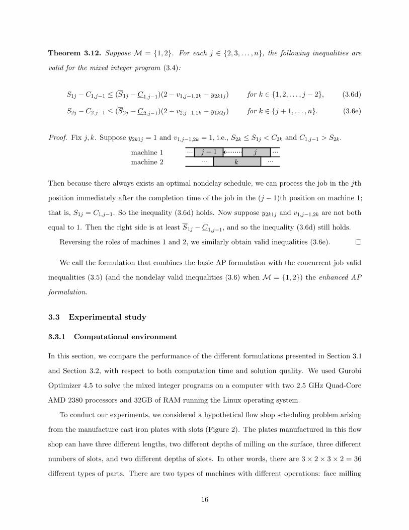
Theorem 3.12. Suppose M = 1, 2. For each j ∈ 2, 3, . . . , n, the following inequalities are
valid for the mixed integer program (3.4):
S1j − C1,j−1 ≤ (S1j − C1,j−1)(2− v1,j−1,2k − y2k1j) for k ∈ 1, 2, . . . , j − 2, (3.6d)
S2j − C2,j−1 ≤ (S2j − C2,j−1)(2− v2,j−1,1k − y1k2j) for k ∈ j + 1, . . . , n. (3.6e)
Proof. Fix j, k. Suppose y2k1j = 1 and v1,j−1,2k = 1, i.e., S2k ≤ S1j < C2k and C1,j−1 > S2k.
...
...
...
...j − 1 j
k
machine 1
machine 2
Then because there always exists an optimal nondelay schedule, we can process the job in the jth
position immediately after the completion time of the job in the (j − 1)th position on machine 1;
that is, S1j = C1,j−1. So the inequality (3.6d) holds. Now suppose y2k1j and v1,j−1,2k are not both
equal to 1. Then the right side is at least S1j − C1,j−1, and so the inequality (3.6d) still holds.
Reversing the roles of machines 1 and 2, we similarly obtain valid inequalities (3.6e).
We call the formulation that combines the basic AP formulation with the concurrent job valid
inequalities (3.5) (and the nondelay valid inequalities (3.6) when M = 1, 2) the enhanced AP
formulation.
3.3 Experimental study
3.3.1 Computational environment
In this section, we compare the performance of the different formulations presented in Section 3.1
and Section 3.2, with respect to both computation time and solution quality. We used Gurobi
Optimizer 4.5 to solve the mixed integer programs on a computer with two 2.5 GHz Quad-Core
AMD 2380 processors and 32GB of RAM running the Linux operating system.
To conduct our experiments, we considered a hypothetical flow shop scheduling problem arising
from the manufacture cast iron plates with slots (Figure 2). The plates manufactured in this flow
shop can have three different lengths, two different depths of milling on the surface, three different
numbers of slots, and two different depths of slots. In other words, there are 3 × 2 × 3 × 2 = 36
different types of parts. There are two types of machines with different operations: face milling
16

Figure 2: Cast iron plates with slots.
and profile milling. We consider two different cases: in the first case, each plate must have the two
operations on one side; in the second case, each plate must have the two operations on two sides.
We can view these two different cases as two different flow shop problems with 2 and 4 machines,
respectively; that is, M = 1, 2 or M = 1, 2, 3, 4. There are five available cutting speeds on
each machine; that is, d = 5 and S = s1, s2, s3, s4, s5. We also consider a special case in which
we can only use each machine’s minimum and maximum speeds; that is, d = 2 and S = s1, s2.
The processing times pijs and power consumption values qijs are generated in accordance with the
Machinery’s Handbook (Oberg et al. 2008). In the instances we study, the processing times pijs are
in the interval [4, 22] (in minutes), and the power consumption values qijs are in the interval [4, 9]
(in kW). For this study, we consider instances in which the number of jobs n is 8, 12, 16, or 20.
We generate 10 different settings for each combination of (m,n, d), by randomly sampling n
jobs with replacement from the 36 job types. Let (m,n, d, k) denote the kth setting that has m
machines, n jobs and d speeds. In summary, the family of settings we use in our experiment is
(2, n, 2, k), (2, n, 5, k), (4, n, 2, k) : n ∈ 8, 12, 16, 20, k ∈ 1, 2, . . . , 10.
For each setting (m,n, d, k), we define Q = maxi∈M,j∈J qij1 and Q =∑
i∈Mmaxj∈J qijd. Note
that when Qmax < Q, there is no feasible schedule, and when Qmax > Q, all jobs can be processed
concurrently at their maximum speed. We call [Q,Q] the power consumption range for each instance,
which we divide into 9 subintervals with same length. For each setting (m,n, d, k), we solve the
corresponding mixed integer program using the 10 endpoints of these subintervals as the threshold
Qmax on the total power consumption at any time instant. This way, for each combination of m,n
and d, we will test 10 settings with 10 different peak power consumption thresholds, or 100 instances
17
of the problem. We set a 30 minute time limit on each instance. For each instance, we provide
Gurobi Optimizer with an upper bound on the optimal makespan, using the best solution obtained
from the two heuristic algorithms described next.
3.3.2 Two heuristic algorithms for finding feasible schedules
For an instance (m,n, d, k) with threshold Qmax on the peak power consumption, let s∗ij be the
maximum possible speed at which job j can be processed on machine i individually without
violating the power consumption threshold; i.e., s∗ij = maxs ∈ S : qijs ≤ Qmax. Suppose we fix
a permutation of the job set. Then one straightforward algorithm (Algorithm 3.1) for finding a
feasible schedule is to process each job j on machine i at speed s∗ij without overlap – that is, with
no other concurrently running jobs.
Algorithm 3.1 Maximum possible speed, fix permutation, no overlap
1: Given pijs, qijs for i ∈M, j ∈ J , s ∈ S, permutation (1, . . . , n) of J2: for j = 1 to n do3: for i = 1 to m do4: calculate s∗ij5: schedule job j on machine i with s∗ij without overlap6: end for7: end for
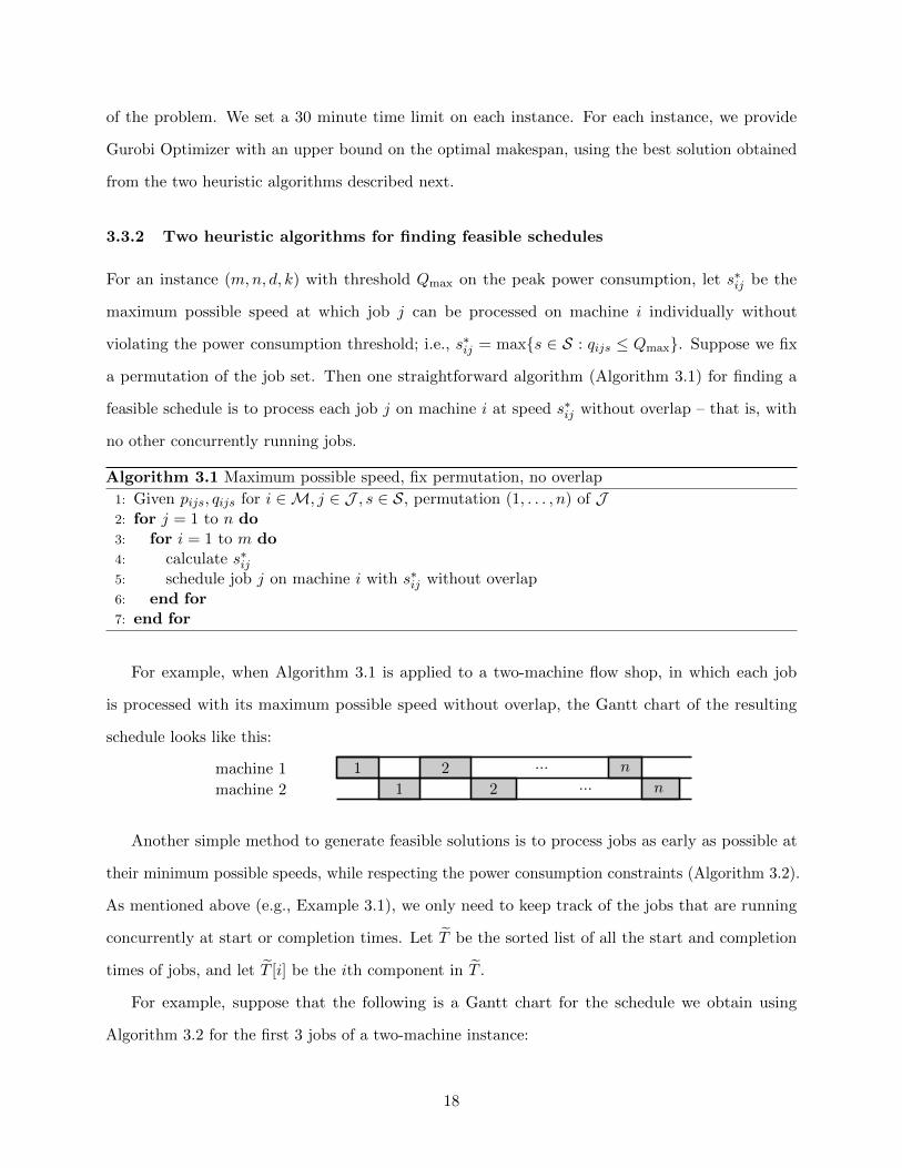
For example, when Algorithm 3.1 is applied to a two-machine flow shop, in which each job
is processed with its maximum possible speed without overlap, the Gantt chart of the resulting
schedule looks like this:
1
1
2
2
...
...n
nmachine 1
machine 2
Another simple method to generate feasible solutions is to process jobs as early as possible at
their minimum possible speeds, while respecting the power consumption constraints (Algorithm 3.2).
As mentioned above (e.g., Example 3.1), we only need to keep track of the jobs that are running
concurrently at start or completion times. Let T be the sorted list of all the start and completion
times of jobs, and let T [i] be the ith component in T .
For example, suppose that the following is a Gantt chart for the schedule we obtain using
Algorithm 3.2 for the first 3 jobs of a two-machine instance:
18

Algorithm 3.2 Minimum possible speed, fix permutation, as early as possible
1: Given pijs, qijs for i ∈M, j ∈ J , s ∈ S, permutation (1, . . . , n) of J2: for j = 1 to n do3: for i = 1 to m do4: schedule job j on machine i at its earliest possible time T [l]5: while power consumption constraints are violated do6: l = l + 17: schedule j on machine i at the next available time T [l]8: end while9: update T
10: end for11: end for
1
1
2 3 4
2 3
t1 t2 t3 t4 t5 t6 t7
machine 1
machine 2
T
Here, T = t1, . . . , t7. Next, Algorithm 3.2 attempts to schedule job 4 on machine 1 at its earliest
possible time t4. If the power consumption threshold is violated when job 4 is processed on machine 1
at time t4, then the algorithm tries to schedule job 4 on machine 1 at the next possible time t5. If
the power consumption threshold is satisfied, then the algorithm schedules job 4 on machine 1 at t5
and updates the list of times T .
The primary role of the two heuristic algorithms described above in our study is to quickly
obtain an upper bound on the optimal makespan for use in Gurobi’s branch-and-cut procedure.
Unfortunately, in our computational results, we found that these upper bounds often are quite loose,
since they only consider processing the jobs at the minimum and maximum speeds available. When
jobs can be processed at a variety of speeds, the schedules found by the heuristic algorithms usually
do not compare well to optimal schedules.
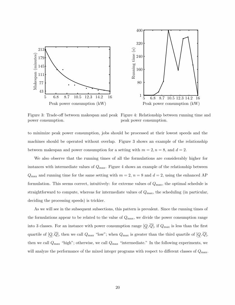
3.3.3 Experiment 1: makespan (Cmax) vs. power consumption (Qmax)
From Assumption 2.1, we know that when a job is processed at a higher speed, its processing
time decreases, while its power consumption increases. Based on this assumption, one expects
a significant trade-off between makespan and peak power consumption. To achieve the shortest
possible makespan, jobs should be processed at their highest possible speeds simultaneously without
idle time, which leads to high peak power consumption. On the other hand, if the objective is
19
Peak power consumption (kW)
Make
span
(min
ute
s)
5 6.8 8.7 10.5 12.3 14.2 16
43
77
111
145
179
213
Figure 3: Trade-off between makespan and peakpower consumption.
Peak power consumption (kW)
Ru
nn
ing
tim
e(s
)
5 6.8 8.7 10.5 12.3 14.2 161
80
160
240
320
400
Figure 4: Relationship between running time andpeak power consumption.
to minimize peak power consumption, jobs should be processed at their lowest speeds and the
machines should be operated without overlap. Figure 3 shows an example of the relationship
between makespan and power consumption for a setting with m = 2, n = 8, and d = 2.
We also observe that the running times of all the formulations are considerably higher for
instances with intermediate values of Qmax. Figure 4 shows an example of the relationship between
Qmax and running time for the same setting with m = 2, n = 8 and d = 2, using the enhanced AP
formulation. This seems correct, intuitively: for extreme values of Qmax, the optimal schedule is
straightforward to compute, whereas for intermediate values of Qmax, the scheduling (in particular,
deciding the processing speeds) is trickier.
As we will see in the subsequent subsections, this pattern is prevalent. Since the running times of
the formulations appear to be related to the value of Qmax, we divide the power consumption range
into 3 classes. For an instance with power consumption range [Q,Q], if Qmax is less than the first
quartile of [Q,Q], then we call Qmax “low”; when Qmax is greater than the third quartile of [Q,Q],
then we call Qmax “high”; otherwise, we call Qmax “intermediate.” In the following experiments, we
will analyze the performance of the mixed integer programs with respect to different classes of Qmax.
20

3.3.4 Experiment 2: disjunctive vs. basic AP formulation
In order to compare the performance of the different formulations, we use the following measures to
assess their performance:
• The number of instances solved to optimality within the 30 minute time limit.
• The average and maximum solution time for these instances solved to optimality.
• The average and maximum speedup factor of the running time for these instances solved to
optimality. For any two formulations a and b, we define the speedup factor (SF) between
a and b for a given instance as the ratio between the times taken for a and b to solve the
instance. We only compute a speedup factor when both formulations can solve the instances
to optimality within the predetermined time limit.
• The average optimality gap at various time points within the 30 minute time limit. We
define the optimality gap as the ratio of the value of the best known feasible solution to the
best known lower bound. This measure lets us compare the performance of the different
formulations for the instances that do not solve to optimality within the time limit.
These performance measures were also used by Keha et al. (2009) and Unlu and Mason (2010) in
their study of mixed integer programming formulations for various scheduling problems.
In this experiment, we compare the performance of the disjunctive and basic AP formulations.
We look at a family of instances similarly constructed to the one described in Section 3.3.1, except
that we look at settings with m = 2, n ∈ 4, 5, 6, 7, 8, and d = 2. We focus on these smaller
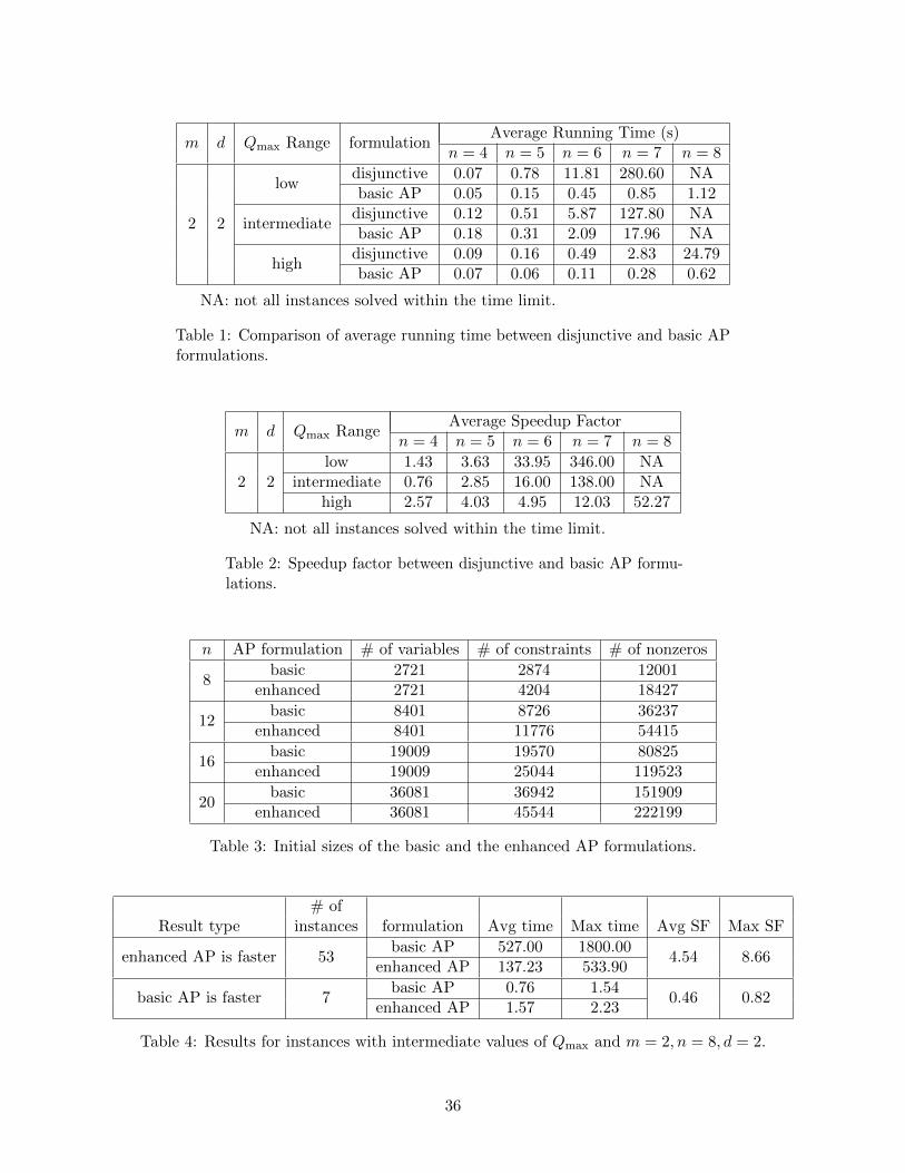
instances in this experiment because as we see in Table 1 (on page 36), the disjunctive formulation
for even moderately sized instances (e.g., n = 8) fails to solve within the 30 minute time limit.
Table 1 shows the average running time for the disjunctive and basic AP formulations, and Table 2
shows the average speedup factor between the disjunctive and basic AP formulations.
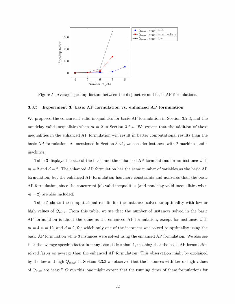
From Tables 1 and 2, we can see that the basic AP formulation runs much faster than the
disjunctive formulation, especially for instances with larger numbers of jobs. Figure 5 graphically
shows the average speedup factor between the disjunctive and basic AP formulations. Given
these observations, we decided to devote more attention to strengthened versions of the basic AP
formulation.
21
4 5 6 7 8
0
100
200
300
Number of jobs
Sp
eedup
fact
or
Qmax range: highQmax range: intermediateQmax range: low
Figure 5: Average speedup factors between the disjunctive and basic AP formulations.
3.3.5 Experiment 3: basic AP formulation vs. enhanced AP formulation
We proposed the concurrent valid inequalities for basic AP formulation in Section 3.2.3, and the
nondelay valid inequalities when m = 2 in Section 3.2.4. We expect that the addition of these
inequalities in the enhanced AP formulation will result in better computational results than the
basic AP formulation. As mentioned in Section 3.3.1, we consider instances with 2 machines and 4
machines.
Table 3 displays the size of the basic and the enhanced AP formulations for an instance with
m = 2 and d = 2. The enhanced AP formulation has the same number of variables as the basic AP
formulation, but the enhanced AP formulation has more constraints and nonzeros than the basic
AP formulation, since the concurrent job valid inequalities (and nondelay valid inequalities when
m = 2) are also included.
Table 5 shows the computational results for the instances solved to optimality with low or
high values of Qmax. From this table, we see that the number of instances solved in the basic
AP formulation is about the same as the enhanced AP formulation, except for instances with
m = 4, n = 12, and d = 2, for which only one of the instances was solved to optimality using the
basic AP formulation while 3 instances were solved using the enhanced AP formulation. We also see
that the average speedup factor in many cases is less than 1, meaning that the basic AP formulation
solved faster on average than the enhanced AP formulation. This observation might be explained
by the low and high Qmax: in Section 3.3.3 we observed that the instances with low or high values
of Qmax are “easy.” Given this, one might expect that the running times of these formulations for
22
these instances are mainly based on the size of the formulations, not the scheduling decisions.
Table 6 shows the computational results for the instances with intermediate values of Qmax.
From this table, we see that in most cases, the average speedup factor is larger than 1. In other
words, for these instances with intermediate values of Qmax, the additional valid inequalities in the
enhanced AP formulation help in reducing running times.
When analyzing the data in more detail, we found more evidence that the additional valid
inequalities are effective in reducing running times for instances with intermediate Qmax. Table 4
shows the computational results for instances with intermediate values of Qmax in which m = 2, n = 8,
and d = 2. From Table 4, we see that for most instances, the enhanced AP formulation runs faster
than the basic AP formulation (i.e. 53 out of 60). On the other hand, for instances in which the
basic AP formulation is faster, we see that the average running times for both formulations are
much smaller (less than 2 seconds).
These observations suggest something similar to what we observed with the data in Table 5.
When the problem is easy to solve, the size of formulation is the main factor in the running time,
implying that the basic AP formulation should be faster. Otherwise, when the problem is more
difficult, the valid inequalities added in the enhanced AP formulation significantly reduce the running
time.
We also observed that the majority of instances, especially those with larger m,n, and d, did
not solve within 30 minutes, even using the enhanced AP formulation. Tables 7, 8 and 9 show the
optimality gap at various times for those instances with both AP formulations within the 30 minute
time limit. From Tables 7, 8 and 9, we see that the valid inequalities help in reducing the optimality
gap of the mixed integer program at various time points in the solution process (especially at the
later times). In addition, we see that as the number of jobs increases, the solution quality decreases
at any given time, since the increased number of jobs adds to the difficulty of scheduling jobs.
4 Two machines, discrete speeds, and zero intermediate storage
Recall that in Problem 2.3, we are given a discrete speed set S = s1, . . . , sd and a set of two
machines M = 1, 2, and there is zero intermediate storage in the flow shop. We will show that
this variant of the PFSPP problem can be transformed into an instance of the asymmetric traveling
23
salesperson problem (TSP). Recall that in the asymmetric TSP, we are given a complete directed
graph and arc distances, and the task is to find a shortest tour in the graph. This transformation
is inspired by a similar transformation of the classic permutation flow shop problem with zero
intermediate storage by Reddi and Ramamoorthy (1972).
Before we describe this transformation, we need to establish the notion of a “block” in a schedule
for a flow shop with no intermediate storage. Consider the following example.
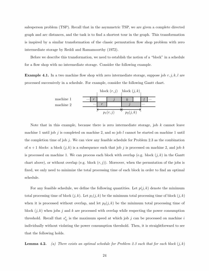
Example 4.1. In a two machine flow shop with zero intermediate storage, suppose job r, j, k, l are
processed successively in a schedule. For example, consider the following Gantt chart.
...
...
...
...r
r
j kj
l
block (r, j) block (j, k)
p1(r, j) p2(j, k)
machine 1
machine 2
Note that in this example, because there is zero intermediate storage, job k cannot leave
machine 1 until job j is completed on machine 2, and so job l cannot be started on machine 1 until
the completion time of job j. We can view any feasible schedule for Problem 2.3 as the combination
of n+ 1 blocks : a block (j, k) is a subsequence such that job j is processed on machine 2, and job k
is processed on machine 1. We can process each block with overlap (e.g. block (j, k) in the Gantt
chart above), or without overlap (e.g. block (r, j)). Moreover, when the permutation of the jobs is
fixed, we only need to minimize the total processing time of each block in order to find an optimal
schedule.
For any feasible schedule, we define the following quantities. Let p(j, k) denote the minimum
total processing time of block (j, k). Let p1(j, k) be the minimum total processing time of block (j, k)
when it is processed without overlap, and let p2(j, k) be the minimum total processing time of
block (j, k) when jobs j and k are processed with overlap while respecting the power consumption
threshold. Recall that s∗ij is the maximum speed at which job j can be processed on machine i
individually without violating the power consumption threshold. Then, it is straightforward to see
that the following holds.
Lemma 4.2. (a) There exists an optimal schedule for Problem 2.3 such that for each block (j, k)
24

of jobs, we have that p1(j, k) = p2js∗2j+ p1ks∗1k
and p2(j, k) = minmaxp2js2j , p1ks1k : q2js2j +
q1ks1k ≤ Qmax, s2j ∈ S, s1k ∈ S.
(b) There exists an optimal schedule for Problem 2.3 such that for each block (j, k) of jobs, the
total processing time p(j, k) = minp1(j, k), p2(j, k).
Note that p(j, k) is not necessarily equal to p(k, j). Using the above lemma, we obtain the following
result.
Theorem 4.3. Problem 2.3 can be viewed as an instance of the asymmetric traveling salesperson
problem.
Proof. For convenience, we introduce a new job 0 with p10 = p20 = 0, and define p(0, j) = p1js∗1jand
p(j, 0) = p2js∗2jfor j = 1, . . . , n. Denote j0 = jn+1 = 0. Then the makespan of schedule (j1, j2, . . . , jn)
is equal to∑n
i=0 p(ji, ji+1). We construct a complete graph G = (V,E) in which V = 0, 1, . . . , n.
We define the distance from node j to k as Djk = p(j, k) for j, k ∈ 0, . . . , n such that j 6= k, and
Djj = +∞ for j = 0, . . . , n. Then Problem 2.3 is equivalent to finding the shortest tour in G with
arc distances D.
5 Two machines, continuous speeds, and zero intermediate stor-
age
In this section we will consider Problem 2.4, in which the flow shop has two machines with zero
intermediate storage, each machine can process jobs at any speed within a continuous interval, and
the power consumption of a machine processing a job at speed s is sα for some constant α > 1.
Given Qmax as the threshold for peak power consumption, we define smax = (Qmax)1α , and let the
speed set S be the continuous interval [0, smax]. Recall that pij is the work required for job j on
machine i, sij ∈ [0, smax] is the chosen speed to process job j on machine i, and pij/sij is the
processing time of job j on machine i.
5.1 Arbitrary work requirements across machines
Lemma 5.1. In any optimal schedule for Problem 2.4, if job j immediately precedes job k, then
sα1k + sα2j = Qmax = sαmax. Moreover, each block (j, k) with j 6= 0 and k 6= 0 in an optimal schedule
25
is processed with overlap, and C2j = C1k.
Proof. Note that at any time, the total power consumption of the two machines must be exactly
Qmax; otherwise we can increase the speeds of the jobs on the two machines so that the total power
consumption is Qmax, and decrease the makespan.
Consider a block (j, k) with j 6= 0 and k 6= 0 in an optimal schedule. If block (j, k) is
processed without overlap in the optimal schedule, then job j and k must be processed at the
maximum speed smax. That is, the minimum total processing time for block (j, k) without overlap
is p1(j, k) =p2j+p1k
(Qmax)1α
.
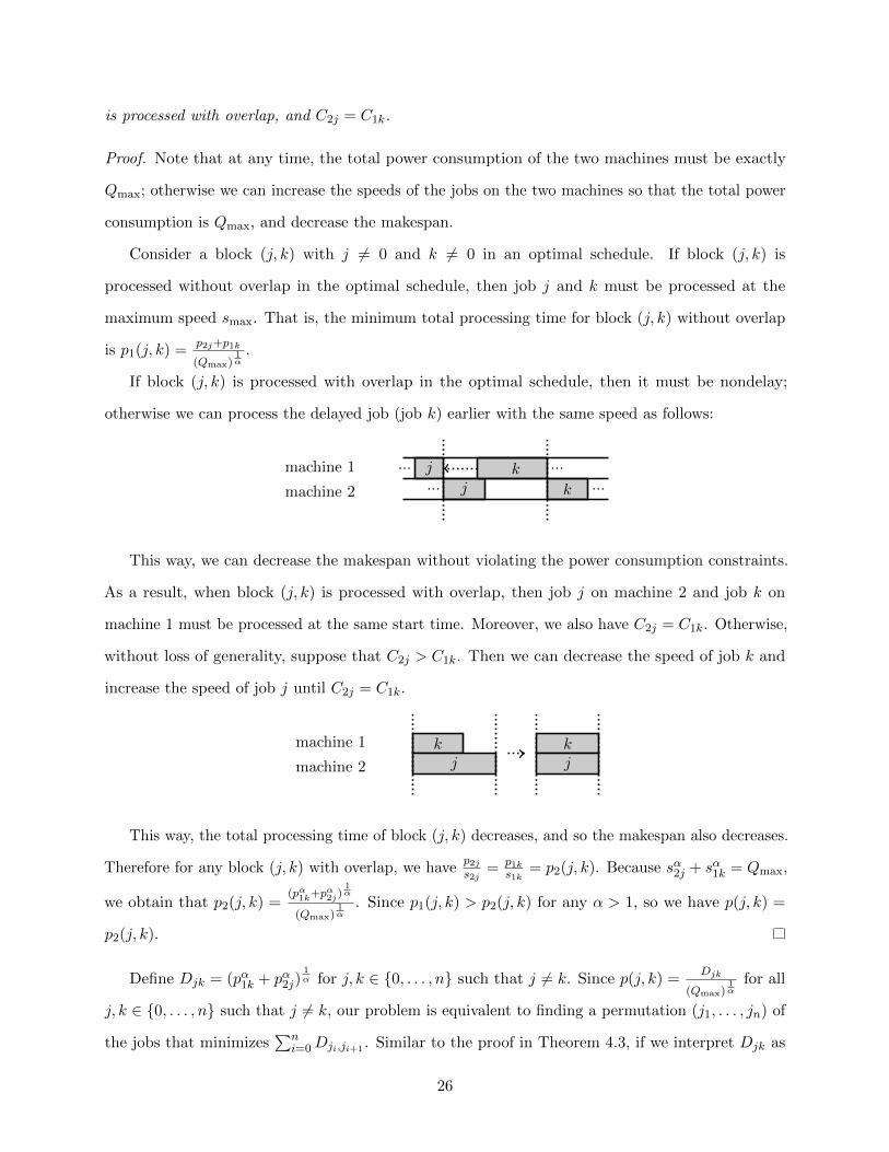
If block (j, k) is processed with overlap in the optimal schedule, then it must be nondelay;
otherwise we can process the delayed job (job k) earlier with the same speed as follows:
...
... ...
...j
jk
k
machine 1
machine 2
This way, we can decrease the makespan without violating the power consumption constraints.
As a result, when block (j, k) is processed with overlap, then job j on machine 2 and job k on
machine 1 must be processed at the same start time. Moreover, we also have C2j = C1k. Otherwise,
without loss of generality, suppose that C2j > C1k. Then we can decrease the speed of job k and
increase the speed of job j until C2j = C1k.
kj
machine 1
machine 2
kj
This way, the total processing time of block (j, k) decreases, and so the makespan also decreases.
Therefore for any block (j, k) with overlap, we havep2js2j
= p1ks1k
= p2(j, k). Because sα2j + sα1k = Qmax,
we obtain that p2(j, k) =(pα1k+pα2j)
1α
(Qmax)1α
. Since p1(j, k) > p2(j, k) for any α > 1, so we have p(j, k) =
p2(j, k).
Define Djk = (pα1k + pα2j)1α for j, k ∈ 0, . . . , n such that j 6= k. Since p(j, k) =
Djk
(Qmax)1α
for all
j, k ∈ 0, . . . , n such that j 6= k, our problem is equivalent to finding a permutation (j1, . . . , jn) of
the jobs that minimizes∑n
i=0Dji,ji+1 . Similar to the proof in Theorem 4.3, if we interpret Djk as
26
the distance of the arc from node j to node k in a complete directed graph on 0, 1, . . . , n, and
define Djj = +∞ for j = 0, . . . , n, then this variant of the PFSPP problem is also a special case of
the asymmetric TSP.
5.2 Consistent work requirements across machines
Although the asymmetric TSP is an NP-hard problem, many of its special cases can be solved
efficiently in polynomial time. One such special case is when the arc distances satisfy the so-called
Demidenko conditions, which state that the matrix D ∈ R(n+1)×(n+1) of arc distances satisfies the
following conditions: for all i, j, l ∈ 0, 1, . . . , n such that i < j < j + 1 < l, we have
Dij +Dj,j+1 +Dj+1,l ≤ Di,j+1 +Dj+1,j +Djl, (5.1)
Dl,j+1 +Dj+1,j +Dji ≤ Dlj +Dj,j+1 +Dj+1,i, (5.2)
Dij +Dl,j+1 ≤ Dlj +Di,j+1, (5.3)
Dji +Dj+1,l ≤ Djl +Dj+1,i. (5.4)
We say that a tour on cities 0, 1, . . . , n is pyramidal if it is of the form (0, i1, . . . , ir, n, j1, . . . , jn−r−1),
where i1 < i2 < · · · < ir and j1 > j2 > · · · > jn−r−1. Demidenko (1979) showed the following for
the asymmetric TSP.
Theorem 5.2 (Demidenko 1979). If D ∈ R(n+1)×(n+1) satisfies the Demidenko conditions, then for
any tour there exists a pyramidal tour of no greater cost. Moreover, a minimum cost pyramidal tour
can be determined in O(n2) time.
Coming back to Problem 2.4, suppose the work requirement of jobs is consistent across machines:
that is, for any two jobs j, k ∈ J , we have that p1j ≤ p1k implies p2j ≤ p2k. Then we have the
following theorem.
Theorem 5.3. If the work required is consistent across machines, then there exists an optimal
schedule for Problem 2.4 that corresponds to a pyramidal TSP tour, and such a schedule can be
found in O(n2) time.
Proof. Fix i, j, l ∈ 0, 1, . . . , n such that i < j < j + 1 < l. Without loss of generality, suppose
p11 ≤ p12 ≤ · · · ≤ p1n and p21 ≤ p22 ≤ · · · ≤ p2n. We can do this since the work is assumed to
27
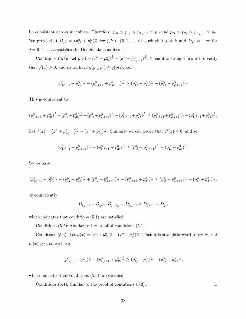
be consistent across machines. Therefore, p1i ≤ p1j ≤ p1,j+1 ≤ p1l and p2i ≤ p2j ≤ p2,j+1 ≤ p2l.
We prove that Djk = (pα1k + pαij)1α for j, k ∈ 0, 1, . . . , n such that j 6= k and Djj = +∞ for
j = 0, 1, . . . , n satisfies the Demidenko conditions.
Conditions (5.1): Let g(x) = (xα + pα2i)1α − (xα + pα2,j+1)
1α . Then it is straightforward to verify
that g′(x) ≥ 0, and so we have g(p1,j+1) ≥ g(p1j), i.e.
(pα1,j+1 + pα2i)1α − (pα1,j+1 + pα2,j+1)
1α ≥ (pα1j + pα2i)
1α − (pα1j + pα2,j+1)
1α .
This is equivalent to
(pα1,j+1 + pα2i)1α −(pα1j+pα2i)
1α +(pα1j+pα2,j+1)
1α −(pα1,j+1 +pα2j)
1α ≥ (pα1,j+1 +pα2,j+1)
1α −(pα1,j+1 +pα2j)
1α .
Let f(x) = (xα + pα2,j+1)1α − (xα + pα2j)
1α . Similarly we can prove that f ′(x) ≤ 0, and so
(pα1,j+1 + pα2,j+1)1α − (pα1,j+1 + pα2j)
1α ≥ (pα1l + pα2,j+1)
1α − (pα1l + pα2j)
1α .
So we have
(pα1,j+1 + pα2i)1α − (pα1j + pα2i)
1α + (pα1j + pα2,j+1)
1α − (pα1,j+1 + pα2j)
1α ≥ (pα1l + pα2,j+1)
1α − (pα1l + pα2j)
1α ,
or equivalently
Di,j+1 −Dij +Dj+1,j −Dj,j+1 ≥ Dj+1,l −Djl,
which indicates that conditions (5.1) are satisfied.
Conditions (5.2): Similar to the proof of conditions (5.1).
Conditions (5.3): Let h(x) = (xα + pα2i)1α − (xα + pα2l)
1α . Then it is straightforward to verify that
h′(x) ≥ 0, so we have
(pα1,j+1 + pα2i)1α − (pα1,j+1 + pα2l)
1α ≥ (pα1j + pα2i)
1α − (pα1j + pα2l)
1α ,
which indicates that conditions (5.3) are satisfied.
Conditions (5.4): Similar to the proof of conditions (5.3).
28
In general, it may be the case that different jobs have their own speed ranges and power functions
(e.g. Bansal et al. 2009). In other words, it may be the case that each job j has a power function
of the form ajsαj + cj , where sj ∈ [smin
j , smaxj ] , Sj . Under this environment, we may obtain
different functions p(j, k) with respect to p1k and p2j for each block (j, k) in Problem 2.4. Using the
Demidenko conditions, we can extend Theorem 5.3 as follows.
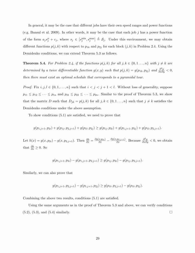
Theorem 5.4. For Problem 2.4, if the functions p(j, k) for all j, k ∈ 0, 1 . . . , n with j 6= k are
determined by a twice differentiable function g(x, y) such that p(j, k) = g(p1k, p2j) and ∂2g∂x∂y < 0,
then there must exist an optimal schedule that corresponds to a pyramidal tour.
Proof. Fix i, j, l ∈ 0, 1, . . . , n such that i < j < j + 1 < l. Without loss of generality, suppose
p11 ≤ p12 ≤ · · · ≤ p1n and p21 ≤ p22 ≤ · · · ≤ p2n. Similar to the proof of Theorem 5.3, we show
that the matrix D such that Djk = p(j, k) for all j, k ∈ 0, 1 . . . , n such that j 6= k satisfies the
Demidenko conditions under the above assumption.
To show conditions (5.1) are satisfied, we need to prove that
g(p1,j+1, p2i) + g(p1j , p2,j+1) + g(p1l, p2j) ≥ g(p1j , p2i) + g(p1,j+1, p2j) + g(p1l, p2,j+1).
Let h(x) = g(x, p2i)− g(x, p2,j+1). Then ∂h∂x = ∂g(x,p2i)
∂x − ∂g(x,p2,j+1)∂x . Because ∂2g
∂x∂y < 0, we obtain
that ∂h∂x ≥ 0. So
g(p1,j+1, p2i)− g(p1,j+1, p2,j+1) ≥ g(p1j , p2i)− g(p1j , p2,j+1).
Similarly, we can also prove that
g(p1,j+1, p2,j+1)− g(p1,j+1, p2j) ≥ g(p1l, p2,j+1)− g(p1l, p2j).
Combining the above two results, conditions (5.1) are satisfied.
Using the same arguments as in the proof of Theorem 5.3 and above, we can verify conditions
(5.2), (5.3), and (5.4) similarly.
29
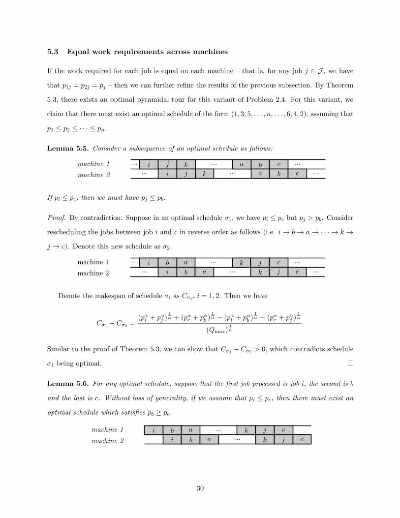
5.3 Equal work requirements across machines
If the work required for each job is equal on each machine – that is, for any job j ∈ J , we have
that p1j = p2j = pj – then we can further refine the results of the previous subsection. By Theorem
5.3, there exists an optimal pyramidal tour for this variant of Problem 2.4. For this variant, we
claim that there must exist an optimal schedule of the form (1, 3, 5, . . . , n, . . . , 6, 4, 2), assuming that
p1 ≤ p2 ≤ · · · ≤ pn.
Lemma 5.5. Consider a subsequence of an optimal schedule as follows:
...
......
...
...
...i j k a b c
i j k a b c
machine 1
machine 2
If pi ≤ pc, then we must have pj ≤ pb.
Proof. By contradiction. Suppose in an optimal schedule σ1, we have pi ≤ pc but pj > pb. Consider
rescheduling the jobs between job i and c in reverse order as follows (i.e. i→ b→ a→ · · · → k →
j → c). Denote this new schedule as σ2.
...
......
...
...
...i b a k j c
i b a k j c
machine 1
machine 2
Denote the makespan of schedule σi as Cσi , i = 1, 2. Then we have
Cσ1 − Cσ2 =(pαi + pαj )
1α + (pαc + pαb )
1α − (pαi + pαb )
1α − (pαc + pαj )
1α
(Qmax)1α
.
Similar to the proof of Theorem 5.3, we can show that Cσ1 − Cσ2 > 0, which contradicts schedule
σ1 being optimal.
Lemma 5.6. For any optimal schedule, suppose that the first job processed is job i, the second is b
and the last is c. Without loss of generality, if we assume that pi ≤ pc, then there must exist an
optimal schedule which satisfies pb ≥ pc.
...
...i b a k j c
i b a k j c
machine 1
machine 2
30
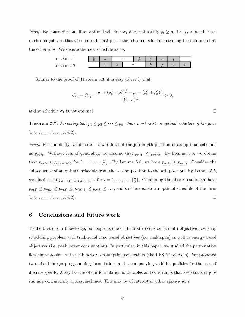
Proof. By contradiction. If an optimal schedule σ1 does not satisfy pb ≥ pc, i.e. pb < pc, then we
reschedule job i so that i becomes the last job in the schedule, while maintaining the ordering of all
the other jobs. We denote the new schedule as σ2:
...
...b a k j c i
b a k j c i
machine 1
machine 2
Similar to the proof of Theorem 5.3, it is easy to verify that
Cσ1 − Cσ2 =pc + (pαi + pαb )
1α − pb − (pαi + pαc )
1α
(Qmax)1α
> 0,
and so schedule σ1 is not optimal.
Theorem 5.7. Assuming that p1 ≤ p2 ≤ · · · ≤ pn, there must exist an optimal schedule of the form
(1, 3, 5, . . . , n, . . . , 6, 4, 2).
Proof. For simplicity, we denote the workload of the job in jth position of an optimal schedule
as pσ(j). Without loss of generality, we assume that pσ(1) ≤ pσ(n). By Lemma 5.5, we obtain
that pσ(i) ≤ pσ(n−i+1) for i = 1, . . . , bn2 c. By Lemma 5.6, we have pσ(2) ≥ pσ(n). Consider the
subsequence of an optimal schedule from the second position to the nth position. By Lemma 5.5,
we obtain that pσ(i+1) ≥ pσ(n−i+1) for i = 1, . . . , . . . , bn2 c. Combining the above results, we have
pσ(1) ≤ pσ(n) ≤ pσ(2) ≤ pσ(n−1) ≤ pσ(3) ≤ . . . , and so there exists an optimal schedule of the form
(1, 3, 5, . . . , n, . . . , 6, 4, 2).
6 Conclusions and future work
To the best of our knowledge, our paper is one of the first to consider a multi-objective flow shop
scheduling problem with traditional time-based objectives (i.e. makespan) as well as energy-based
objectives (i.e. peak power consumption). In particular, in this paper, we studied the permutation
flow shop problem with peak power consumption constraints (the PFSPP problem). We proposed
two mixed integer programming formulations and accompanying valid inequalities for the case of
discrete speeds. A key feature of our formulation is variables and constraints that keep track of jobs
running concurrently across machines. This may be of interest in other applications.
31

We investigated the computational performance of these formulations with instances arising from
the manufacture of cast iron plates. Although our valid inequalities for the assignment and positional
formulation resulted in better computational performance, especially for small-to-moderate sized
instances, we still had difficulty obtaining optimal schedules in a reasonable amount of time for
instances with large numbers of jobs and machines. One potential direction for future research
is to develop stronger valid inequalities for our formulations, in the hopes of strengthening these
formulations and improving their computational performance.
We also showed that our scheduling problem can be recast as an asymmetric TSP when the flow
shop has two machines with zero intermediate storage. In addition, we were able to obtain stronger
structural characterizations of optimal schedules and polynomial time algorithms to find these
schedules when the speed set is continuous and the work requirements satisfy certain conditions.
Of course, there are many other possible directions for future research stemming from this work.
For example, the computational complexity of the PFSPP problem remains open when there are two
machines. It would be interesting to fully characterize which two-machine variants of our scheduling
problem are NP-hard or polynomial time solvable. Since minimizing the makespan in an ordinary
permutation flow shop is NP-hard when there are three or more machines (Garey et al. 1976) and
the PFSPP problem can be seen as a special case of this ordinary permutation flow shop problem
(by setting the peak power consumption threshold Qmax sufficiently high), the PFSPP problem is
also NP-hard when there are three or more machines. Another interesting direction would be to
determine when our proposed formulations have strong LP relaxations. Last but not least, it would
also be interesting to consider different time or energy objectives (e.g. total weighted completion
time, carbon footprint) or some other complex machine environments with peak power consumption
constraints.
References
S. Albers. Energy-efficient algorithms. Communications of the ACM, 53(5):86–96, 2010.
C. A. Babu and S. Ashok. Peak load management in electrolytic process industries. IEEE
Transactions on Power Systems, 23(2):399–405, 2008.
32
N. Bansal, T. Kimbrel, and K. Pruhs. Speed scaling to manage energy and temperature. Journal of
the ACM, 54(1):1–39, 2007.
N. Bansal, H. L. Chan, and K. Pruhs. Speed scaling with an arbitrary power function. In Proceedings
of the 20th Annual ACM-SIAM Symposium on Discrete Algorithms, pages 693–701, 2009.
W. Bouzid. Cutting parameter optimization to minimize production time in high speed turning.
Journal of Materials Processing Technology, 161(3):388–395, 2005.
R. Cochran, C. Hankendi, A. Coskun, and S. Reda. Pack & cap: adaptive DVFS and thread packing
under power caps. In Proceedings of the 44th Annual IEEE/ACM International Symposium on
Microarchitecture, 2011.
J. B. Dahmus and T. G. Gutowski. An environmental analysis of machining. In ASME 2004
International Mechanical Engineering Congress and Exposition, pages 643–652, 2004.
V. M. Demidenko. The traveling salesman problem with asymmetric matrices (in Russian). Izvestiya
Akademii Nauk BSSR Seriya, Seryya Fizika-Matehmatychnykh Navuk, pages 29–35, 1979.
R. Drake, M. B. Yildirim, J. Twomey, L. Whitman, J. Ahmad, and P. Lodhia. Data collection
framework on energy comsumption in manufacturing. In IIE Annual Conference and Expo 2006,
2006.
K. Fang, N. A. Uhan, F. Zhao, and J. W. Sutherland. A new approach to scheduling in manufacturing
for power consumption and carbon footprint reduction. Journal of Manufacturing Systems, 30(4):
234–240, 2011.
W. Felter, K. Rajamani, T. Keller, and C. Rusu. A performance-conserving approach for reducing
peak power consumption in server systems. In Proceedings of the 19th Annual International
Conference on Supercomputing, pages 293–302, 2005.
M. R. Garey, D. S. Johnson, and R. Sethi. The complexity of flowshop and jobshop scheduling.
Mathematics of Operations Research, 1(2):117–129, 1976.
T. Gutowski, C. Murphy, D. Allen, D. Bauer, B. Bras, T. Piwonka, P. Sheng, J. Sutherland,
33

D. Thurston, and E. Wolff. Environmentally benign manufacturing: observations from Japan,
Europe and the United States. Journal of Cleaner Production, 13:1–17, 2005.
S. Irani and K. R. Pruhs. Algorithmic problems in power management. SIGACT News, 36(2):63–76,
2005.
A. B. Keha, K. Khowala, and J. W. Fowler. Mixed integer programming formulations for single
machine scheduling problems. Computers & Industrial Engineering, 56(1):357–367, 2009.
V. Kontorinis, A. Shayan, D. M. Tullsen, and R. Kumar. Reducing peak power with a table-driven
adaptive processor core. In Proceedings of the 42nd Annual IEEE/ACM International Symposium
on Microarchitecture, pages 189–200, 2009.
W. C. Kwon and T. Kim. Optimal voltage allocation techniques for dynamically variable voltage
processors. ACM Transactions on Embedded Computing Systems, 4(1):211–230, 2005.
J. B. Lasserre and M. Queyranne. Generic scheduling polyhedra and a new mixed-integer formulation
for single-machine scheduling. In Proceedings of the 2nd IPCO Conference, pages 136–149, 1992.
A. S. Manne. On the job-shop scheduling problem. Operations Research, 8(2):219–223, 1960.
G. Mouzon and M. B. Yildirim. A framework to minimise total energy consumption and total
tardiness on a single machine. International Journal of Sustainable Engineering, 1(2):105–116,
2008.
G. Mouzon, M. B. Yildirim, and J. Twomey. Operational methods for minimization of energy
consumption of manufacturing equipment. International Journal of Production Research, 45
(18-19):4247–4271, 2007.
T. Mudge. Power: A first-class architectural design constraint. Computer, 34(4):52–58, 2001.
E. Oberg, F. D. Jones, H. L. Horton, and H. H. Ryffel. Machinery’s Handbook. Industrial Press,
New York, 28th edition, 2008.
S. S. Reddi and C. V. Ramamoorthy. On the flow-shop sequencing problem with no wait in process.
Operational Research Quarterly, 23(3):323–331, 1972.
34

E. F. Stafford Jr., F. T. Tseng, and J. N. D. Gupta. Comparative evaluation of MILP flowshop
models. Journal of the Operational Research Society, 56:88–101, 2005.
K. Thornblad, A. B. Stromberg, and M. Patriksson. Optimization of schedules for a multitask
production cell. In The 22nd Annual NOFOMA Conference Proceedings, 2010.
Y. Unlu and S. J. Mason. Evaluation of mixed integer programming formulations for non-preemptive
parallel machine scheduling problems. Computers & Industrial Engineering, 58(4):785–800, 2010.
H. M. Wagner. An integer linear-programming model for machine scheduling. Naval Research
Logistics Quarterly, 6(2):134–140, 1959.
F. Yao, A. Demers, and S. Shenker. A scheduling model for reduced CPU energy. In Proceedings of
the 36th Annual Symposium on Foundations of Computer Science, pages 374–382, 1995.
35
m d Qmax Range formulationAverage Running Time (s)
n = 4 n = 5 n = 6 n = 7 n = 8
2 2
lowdisjunctive 0.07 0.78 11.81 280.60 NAbasic AP 0.05 0.15 0.45 0.85 1.12
intermediatedisjunctive 0.12 0.51 5.87 127.80 NAbasic AP 0.18 0.31 2.09 17.96 NA
highdisjunctive 0.09 0.16 0.49 2.83 24.79basic AP 0.07 0.06 0.11 0.28 0.62
NA: not all instances solved within the time limit.
Table 1: Comparison of average running time between disjunctive and basic APformulations.
m d Qmax RangeAverage Speedup Factor
n = 4 n = 5 n = 6 n = 7 n = 8
2 2low 1.43 3.63 33.95 346.00 NA
intermediate 0.76 2.85 16.00 138.00 NAhigh 2.57 4.03 4.95 12.03 52.27
NA: not all instances solved within the time limit.
Table 2: Speedup factor between disjunctive and basic AP formu-lations.
n AP formulation # of variables # of constraints # of nonzeros
8basic 2721 2874 12001
enhanced 2721 4204 18427
12basic 8401 8726 36237
enhanced 8401 11776 54415
16basic 19009 19570 80825
enhanced 19009 25044 119523
20basic 36081 36942 151909
enhanced 36081 45544 222199
Table 3: Initial sizes of the basic and the enhanced AP formulations.
# ofResult type instances formulation Avg time Max time Avg SF Max SF
enhanced AP is faster 53basic AP 527.00 1800.00
4.54 8.66enhanced AP 137.23 533.90
basic AP is faster 7basic AP 0.76 1.54
0.46 0.82enhanced AP 1.57 2.23
Table 4: Results for instances with intermediate values of Qmax and m = 2, n = 8, d = 2.
36

Inst
ance
typ
eb
asic
AP
enh
ance
dA
PA
vg
SF
Max
SF
md
Qm
ax
Ran
ge
#of
inst
ance
sn
#so
lved
Avg
tim
eM
axti
me
#so
lved
Avg
tim
eM
axti
me
22
low
20
820
1.10
1.77
201.
532.
900.
811.
6212
2010
9.70
208.
3020
54.6
788
.64
1.96
3.68
160
--
0-
--
-20
0-
-0
--
--
hig
h20
820
74.8
176
3.14
2025
.25
300.
690.
934.
6312
1929
.98
223.
7819
48.9
040
9.30
0.60
2.98
1618
118.
3213
34.6
318
134.
2479
2.74
0.51
1.68
2018
181.
1112
00.9
217
297.
8813
13.0
10.
533.
34
25
low
20
820
1.64
2.50
202.
003.
890.
891.
7012
2016
0.55
205.
6220
112.
1538
6.55
1.67
2.77
160
--
0-
--
-20
0-
-0
--
--
hig
h20
820
1.58
11.2
020
1.76
3.51
0.83
3.19
1220
8.71
59.6
220
24.0
555
.97
0.41
1.07
1620
19.5
681
.00
2080
.74
213.
360.
401.
7820
2099
.79
514.
1520
249.
4072
3.71
0.56
4.10
42
low
20
80
--
0-
--
-12
0-
-0
--
--
160
--
0-
--
-20
0-
-0
--
--
hig
h20
819
406.
5811
09.0
019
499.
1111
51.8
91.
024.
4412
114
90.8
214
90.8
23
1425
.87
1532
.59
1.20
1.37
160
--
0-
--
-20
0-
-0
--
--
Tab
le5:
Res
ult
sfo
rso
lved
inst
ance
sw
ith
low
orh
ighQ
max.
37

Inst
ance
typ
eb
asic
AP
enh
ance
dA
PA
vg
SF
Max
SF
md
Qm
ax
Ran
ge
#of
inst
an
ces
n#
solv
edA
vg
tim
eM
axti
me
#so
lved
Avg
tim
eM
axti
me
22
inte
rmed
iate
60
859
442.
9916
82.5
160
121.
4153
3.91
4.06
8.66
12
910
3.63
497.
809
66.1
621
0.29
1.87
7.66
16
820
4.69
1172
.95
930
4.31
1452
.12
1.57
7.34
20
835
5.16
889.
057
440.
1513
11.6
70.
811.
74
25
inte
rmed
iate
60
838
270.
2313
53.9
760
390.
0215
91.2
62.
116.
9012
1710
7.08
226.
5618
207.
0213
07.4
60.
751.
5716
1632
9.35
1697
.98
1637
3.06
1314
.90
0.83
1.64
20
560
2.92
800.
105
810.
6116
29.2
81.
072.
28
42
inte
rmed
iate
60
86
550.
6085
1.57
981
1.42
1660
.00
1.17
1.73
12
0-
-0
--
--
16
0-
-0
--
--
20
0-
-0
--
--
Tab
le6:
Res
ult
sfo
rso
lved
inst
ance
sw
ith
inte
rmed
iateQ
max.
38

Inst
ance
typ
eA
Pfo
rmu
lati
ons
Ave
rage
opti
mal
ity
gap
atti
met
(s)
md
Qm
ax
Ran
ge
n5
1030
6015
030
060
012
0018
00
22
low
8b
asic
1.00
1.00
1.00
1.00
1.00
1.00
1.00
1.00
1.00
enh
ance
d1.
001.
001.
001.
001.
001.
001.
001.
001.
00
12b
asic
1.39
1.31
1.24
1.12
1.02
1.00
1.00
1.00
1.00
enh
ance
d1.
381.
281.
171.
041.
001.
001.
001.
001.
00
16b
asic
1.61
1.56
1.48
1.47
1.41
1.36
1.31
1.27
1.24
enh
ance
d1.
601.
541.
461.
431.
361.
311.
271.
221.
20
20b
asic
1.65
1.63
1.60
1.57
1.55
1.53
1.50
1.47
1.46
enh
ance
d1.
651.
631.
591.
561.
531.
501.
471.
441.
43
inte
rmed
iate
8b
asic
1.38
1.34
1.25
1.19
1.11
1.06
1.02
1.01
1.00
enh
ance
d1.
321.
251.
131.
081.
031.
011.
001.
001.
00
12b
asic
1.55
1.46
1.43
1.40
1.36
1.34
1.30
1.28
1.27
enh
ance
d1.
641.
471.
411.
361.
311.
281.
251.
211.
20
16b
asic
1.66
1.65
1.50
1.48
1.43
1.40
1.38
1.37
1.37
enh
ance
d1.
681.
671.
511.
501.
421.
381.
361.
341.
33
20b
asic
1.70
1.70
1.67
1.52
1.49
1.45
1.43
1.41
1.40
enh
ance
d1.
701.
701.
701.
591.
541.
451.
421.
401.
39
hig
h
8b
asic
1.03
1.02
1.01
1.01
1.01
1.01
1.01
1.00
1.00
enh
ance
d1.
021.
021.
011.
011.
001.
001.
001.
001.
00
12b
asic
1.08
1.06
1.03
1.02
1.02
1.01
1.01
1.01
1.01
enh
ance
d1.
301.
091.
061.
021.
021.
011.
011.
011.
01
16b
asic
1.40
1.28
1.09
1.05
1.02
1.02
1.02
1.01
1.01
enh
ance
d1.
641.
541.
191.
451.
031.
021.
011.
011.
01
20b
asic
1.69
1.62
1.29
1.11
1.05
1.02
1.01
1.01
1.00
enh
ance
d1.
721.
721.
651.
331.
191.
031.
011.
011.
00
Tab
le7:
Aver
age
opti
mal
ity
gap
for
inst
ance
sw
ithm
=2,d
=2.
39

Inst
ance
typ
eA
Pfo
rmu
lati
ons
Ave
rage
opti
mal
ity
gap
atti
met
(s)
md
Qm
ax
Ran
ge
n5
1030
6015
030
060
012
0018
00
25
low
8b
asic
1.00
1.00
1.00
1.00
1.00
1.00
1.00
1.00
1.00
enh
ance
d1.
001.
001.
001.
001.
001.
001.
001.
001.
00
12b
asic
1.51
1.40
1.35
1.26
1.08
1.00
1.00
1.00
1.00
enh
ance
d1.
581.
411.
301.
191.
021.
011.
001.
001.
00
16b
asic
1.74
1.70
1.59
1.56
1.51
1.45
1.40
1.36
1.34
enh
ance
d1.
771.
731.
571.
531.
471.
411.
361.
311.
29
20b
asic
1.77
1.76
1.73
1.69
1.66
1.62
1.58
1.55
1.53
enh
ance
d1.
781.
781.
711.
661.
631.
591.
551.
511.
50
inte
rmed
iate
8b
asic
1.38
1.36
1.24
1.20
1.15
1.11
1.07
1.05
1.04
enh
ance
d1.
391.
351.
201.
141.
081.
061.
031.
001.
00
12b
asic
1.80
1.64
1.48
1.44
1.36
1.33
1.30
1.27
1.25
enh
ance
d1.
811.
781.
461.
411.
311.
271.
251.
221.
20
16b
asic
1.81
1.81
1.65
1.48
1.46
1.39
1.36
1.34
1.33
enh
ance
d1.
811.
811.
801.
621.
461.
361.
321.
291.
28
20b
asic
NA
1.84
1.84
1.82
1.54
1.53
1.49
1.43
1.42
enh
ance
dN
A1.
851.
841.
831.
711.
511.
451.
401.
39
hig
h
8b
asic
1.00
1.00
1.00
1.00
1.00
1.00
1.00
1.00
1.00
enh
ance
d1.
001.
001.
001.
001.
001.
001.
001.
001.
00
12b
asic
1.37
1.07
1.01
1.00
1.00
1.00
1.00
1.00
1.00
enh
ance
d1.
811.
471.
031.
001.
001.
001.
001.
001.
00
16b
asic
1.77
1.36
1.03
1.01
1.00
1.00
1.00
1.00
1.00
enh
ance
d1.
811.
811.
601.
081.
001.
001.
001.
001.
00
20b
asic
NA
1.84
1.54
1.17
1.03
1.01
1.00
1.00
1.00
enh
ance
dN
A1.
841.
841.
801.
101.
031.
001.
001.
00
NA
:fo
rth
ese
inst
ance
s,th
ero
otL
Pre
laxat
ion
sof
the
form
ula
tion
sd
idn
otso
lve
inle
ssth
an5s
.
Tab
le8:
Aver
age
opti
mal
ity
gap
for
inst
ance
sw
ithm
=2,d
=5.
40
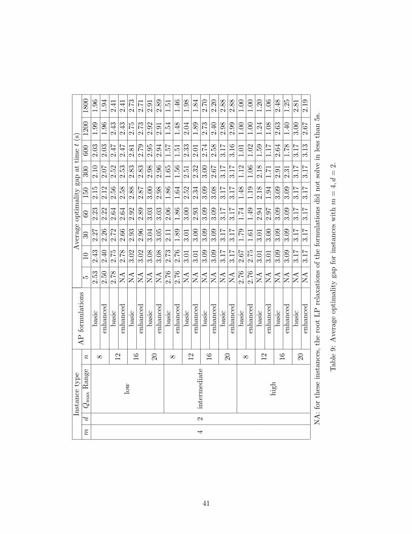
Inst
ance
typ
eA
Pfo
rmu
lati
ons
Ave
rage
opti
mal
ity
gap
atti
met
(s)
md
Qm
ax
Ran
ge
n5
1030
6015
030
060
012
0018
00
42
low
8b
asic
2.53
2.43
2.27
2.23
2.15
2.10
2.03
1.99
1.96
enh
ance
d2.
502.
402.
262.
222.
122.
072.
031.
961.
94
12b
asic
2.78
2.75
2.72
2.64
2.56
2.52
2.47
2.43
2.41
enh
ance
dN
A2.
782.
662.
642.
582.
532.
472.
432.
41
16b
asic
NA
3.02
2.93
2.92
2.88
2.83
2.81
2.75
2.73
enh
ance
dN
A3.
022.
962.
892.
872.
832.
792.
732.
71
20b
asic
NA
3.08
3.04
3.03
3.00
2.98
2.95
2.92
2.91
enh
ance
dN
A3.
083.
053.
032.
982.
962.
942.
912.
89
inte
rmed
iate
8b
asic
2.76
2.73
2.11
2.06
1.86
1.65
1.57
1.54
1.51
enh
ance
d2.
762.
761.
891.
861.
641.
561.
511.
481.
46
12b
asic
NA
3.01
3.01
3.00
2.52
2.51
2.33
2.04
1.98
enh
ance
dN
A3.
013.
002.
932.
342.
322.
011.
891.
84
16b
asic
NA
3.09
3.09
3.09
3.09
3.00
2.74
2.73
2.70
enh
ance
dN
A3.
093.
093.
093.
082.
672.
582.
402.
20
20b
asic
NA
3.17
3.17
3.17
3.17
3.17
3.17
2.98
2.88
enh
ance
dN
A3.
173.
173.
173.
173.
173.
162.
992.
88
hig
h
8b
asic
2.76
2.67
1.79
1.74
1.48
1.12
1.01
1.00
1.00
enh
ance
d2.
762.
751.
611.
491.
191.
061.
021.
001.
00
12b
asic
NA
3.01
3.01
2.94
2.18
2.18
1.59
1.24
1.20
enh
ance
dN
A3.
013.
002.
971.
941.
711.
171.
081.
06
16b
asic
NA
3.09
3.09
3.09
3.09
2.91
2.64
2.63
2.48
enh
ance
dN
A3.
093.
093.
093.
092.
311.
781.
401.
25
20b
asic
NA
3.17
3.17
3.17
3.17
3.17
3.17
3.00
2.81
enh
ance
dN
A3.
173.
173.
173.
173.
173.
132.
672.
19
NA
:fo
rth
ese
inst
ance
s,th
ero
otL
Pre
laxat
ion
sof
the
form
ula
tion
sd
idn
otso
lve
inle
ssth
an5s
.
Tab
le9:
Aver
age
opti
mal
ity
gap
for
inst
ance
sw
ithm
=4,d
=2.
41