flow in thin regions bounded by structured and porous
TRANSCRIPT

University of New MexicoUNM Digital Repository
Chemical and Biological Engineering ETDs Engineering ETDs
1-30-2013
Flow in thin regions bounded by structured andporous surfaces : applications to load bearingsAbishek Venkatakrishnan
Follow this and additional works at: https://digitalrepository.unm.edu/cbe_etds
This Thesis is brought to you for free and open access by the Engineering ETDs at UNM Digital Repository. It has been accepted for inclusion inChemical and Biological Engineering ETDs by an authorized administrator of UNM Digital Repository. For more information, please [email protected].
Recommended CitationVenkatakrishnan, Abishek. "Flow in thin regions bounded by structured and porous surfaces : applications to load bearings." (2013).https://digitalrepository.unm.edu/cbe_etds/40

Candidate Department This thesis is approved, and it is acceptable in quality and form for publication: Approved by the Thesis Committee: , Chairperson

by
THESIS
Submitted in Partial Fulfillment of theRequirements for the Degree of
The University of New MexicoAlbuquerque, New Mexico

iii
DEDICATION
This thesis is dedicated to my late father, C.S. Venkatakrishnan, and my mother, V.K.
Anuradha, for their endless support, love and encouragement.

iv
ACKNOWLEDGEMENTS
I would like to express my sincere gratitude to my advisor Dr. Randy Schunk for his
constant support throughout my Master’s research. His timely guidance, in both academic
and research career, has been invaluable. I have been fortunate enough to work under his
supervision.
I would also like to thank Dr. Kristianto Tjiptowidjojo for his insightful guidance and
comments. I also extend my thanks to the thesis committee members Dr. Dimiter Petsev
and Dr. Scott Roberts.

v
FLOW IN THIN REGIONS BOUNDED BY STRUCTURED AND POROUS
SURFACES: APPLICATIONS TO LOAD BEARINGS
BY
ABISHEK VENKATAKRISHNAN
B.S., CHEMICAL ENGINEERING, 2009
M.S., CHEMICAL ENGINEERING, 2012
ABSTRACT
The effect of surface roughness on the load capacity and friction force of
hydrodynamic bearings has received considerable interest from scientists and
engineers. Surfaces of most engineered materials are textured at some level either
deliberately to achieve some desired effect or produced by wear and friction of
surfaces.
This thesis analyses the effect of surface roughness and porosity on the load
capacity of hydrodynamic bearings. The surface roughness is characterized by a
single sinusoidal wave function. The implementation of sinusoidal roughness
model is verified using a verification problem. Reynolds’ lubrication theory,
derived from thin-region approximations of the Navier-Stokes equations, is used
as the main tool for this study. The performance of a rough slider bearing is
compared with a corresponding smooth slider bearing. The presence of roughness
tends to increase the load capacity of a slider bearing at high amplitudes and low
wavelengths. The level-set method is used to track interfaces for problems
involving multiphase flow. In general, the results show that the surface roughness
influences the pressure distribution and load capacity of bearings.

vi
TABLE OF CONTENTS LIST OF FIGURES ....................................................................................................... viii
LIST OF TABLES ............................................................................................................. x
1. INTRODUCTION .........................................................................................................1
1.1 Tribology ...........................................................................................................1
1.2 Lubrication .........................................................................................................3
1.2.1 Hydrodynamic Lubrication .................................................................6
1.2.2 Reynolds Lubrication Theory .............................................................8
1.2.3 Applications and Examples .................................................................9
1.3 Thesis Overview ..............................................................................................10
2. Effect of Surface Roughness on the Load Capacity of a Slider Bearing .................13
2.1 Introduction ......................................................................................................13
2.2 Theory ..............................................................................................................15
2.3 The Model ........................................................................................................17
2.4 Results and Discussion ....................................................................................20
2.4.1 Sinusoidal Surface - Hydrodynamic Bearing ...................................21
2.4.1 Effect of Sinusoidal Surface Roughness on the Load Capacity of a
Slider Bearing ............................................................................................24
3. Effect of Surface Roughness on the Load Capacity of a Journal
Bearing: Multiphase Flow ...............................................................................................32
3.1 Introduction ......................................................................................................32
3.2 Theory ..............................................................................................................33
3.2.1 Multiphase Flow ...............................................................................33
vii
3.2.2. Level-Set Method .............................................................................35
3.2.3 Implementation in GOMA ................................................................37
3.3 The Model ........................................................................................................38
3.4 Results and Discussions ...................................................................................41
4. Effect of Porosity and Capillary Imbibition on the Load Capacity
of a Porous Journal Bearing ...........................................................................................47
4.1 Introduction ......................................................................................................47
4.2 Theory ..............................................................................................................48
4.3 The Model ........................................................................................................50
4.4 Results and Discussions ...................................................................................51
5. Conclusions and Recommendations for Future Work .............................................53
5.1 Conclusions ......................................................................................................53
5.1.1 Slider Bearing Model ........................................................................53
5.2.2 Multiphase Flow in a Journal Bearing ..............................................54
APPENDIX .......................................................................................................................55
APPENDIX A – COMPARITIVE STUDY OF COATING FLOWS WITH
CONTINUUM AND LUBRICATION MODELS ........................................................55
REFERENCES .................................................................................................................66
viii
LIST OF FIGURES
1.1 Regimes of lubrication: Stribeck curve ..........................................................................4
1.2 (a) Illustration of a slider bearing
(b) Illustration of a journal bearing ................................................................................7
1.3 Tower’s Experimental set-up rig ...................................................................................9
2.1 Schematic diagram of a slider bearing with sinusoidal surface roughness ..................18
2.2 Journal bearing mesh ...................................................................................................21
2.3 Effect of harmonic number on load bearing capacity ..................................................23
2.4 Lubrication approximation validity “window” along with roughness profiles ...........25
2.5 Comparison of load capacity for lubrication formulation and full Navier-Stokes
solutions .............................................................................................................................27
2.6 Effect of wall velocity on load bearing capacity .........................................................29
2.7 Effect of amplitude number on load bearing capacity .................................................30
2.8 Effect of roughness number on load bearing capacity .................................................31
3.1 Journal bearing: Multiphase flow model with coordinate axes ...................................40
3.2 Fingering instability .....................................................................................................42
3.3 Effect of wettability on load capacity ..........................................................................43
3.4 Effect of wettability on load capacity ..........................................................................44
3.5 Effect of wettability on load capacity ..........................................................................44
3.6 Effect of wettability on load capacity ..........................................................................45
4.1 Schematic of a porous journal bearing .........................................................................50
4.2 Effect of porosity and capillary imbibition on load capacity .......................................51
ix
1 Coating flow – Continuum Model ..................................................................................56
2 Coating flow – Lubrication Model .................................................................................59
3 Two-dimensional continuum model with boundary conditions .....................................61
4 Lubrication model along with the inflow and outflow boundary conditions ..................62
5 Effect of film thickness ratio on Capillary number ........................................................64
6 Various mesh layouts ......................................................................................................65
x
LIST OF TABLES
2.1 Design parameters of journal bearing ..........................................................................22
2.2 Bearing load calculations at different harmonic numbers ...........................................22
2.3(a) Table showing amplitude and amplitude number values ........................................24
2.3(b) Table showing wavelength and roughness number values .....................................24
A.1 Film thickness ratios computed at different web speeds and pressures ......................63

1
Chapter 1 Introduction
1.1 Tribology
The word tribology, coined by David Tabor (Jost 1966), is derived from the
Greek word tribos, which roughly translates into study of sliding or rubbing. Modern
dictionaries define tribology as the study that deals with the science and engineering
principles of design, friction, wear, and lubrication of interacting surfaces in relative
motion.
In recent decades, the field of tribology has received considerable of interest even
though it has been topical for centuries. The scientific study of tribology has a long
history which dates back as early as the 15th century. Leonardo Da Vinci is thought to
have been the first to develop the laws of friction, such as the proportionality between
normal force and limiting friction force (Stachowiak and Batchelor (2000)). An in-depth
insight into the history of tribology can be found in Dowson (1997). The complex
problems involving the fundamentals of wear and friction has seen limited progress in
this field of study, especially as much of the relevant physical phenomena occur at micro-
and nanometer length scales. Most progress in understanding of tribology has occurred
since the Second World War, when significant breakthroughs in experimental
instrumentation and theoretical understanding of the underpinning material and
engineering science were made.
Wear can be defined as the gradual deformation and removal of surface material
due to mechanical and relative motion of surfaces. Wear is the major cause of material
damage and reduced performance of mechanical components. According to reports, the

2
estimated annual financial loss due to wear in the USA is 6% - 7% of the total Gross
Domestic Product (GDP) (Seireg 1998). Accordingly, significant scientific and
engineering attention has been devoted to controlling friction. An efficient way to reduce
friction and thereby wear is with lubrication. Lubrication implies the use of a friction-
reducing substance known as a lubricant to aid in reducing mechanical (solid-solid)
contact, reduce energy dissipation into heat, and ultimately reduce wear of surfaces in
relative motion. A lubricant can be a solid, a liquid-solid gel, a liquid or a gas.
Friction is encountered in our lives on a daily basis. For example, when we rub
our hands together, heat is generated due to friction. Other real life examples include
friction between footwear and ground while walking, friction between our fingers and
pen/pencil while writing, friction between tires and ground while driving, friction
between a snow ski and snow, and so forth. Friction is typically characterized in terms of
the coefficient of friction. It is defined as the ratio of the force required to move two
surfaces over each other to the force holding them together.
In short, the objective of the field of tribology is to understand the underpinning
physics (mechanical, thermal, chemistry, etc.) of friction and wear so that it can be
controlled in technologically important problems. In some cases, it is desirable to
minimize wear but maximize friction (e.g. brakes) or minimize friction but not wear or
maximize both wear and friction.

3
1.2 Lubrication
Friction and wear can occur when two surfaces move relative to each other. One
way of reducing friction is with lubrication. Addition of lubricants can significantly
reduce friction and thereby lead to reduction in wear and mechanical energy dissipation
into thermal energy (i.e. heat). A lubricant film can be solid, liquid, liquid-liquid
dispersion, solid-liquid dispersion or gas. The thickness of lubricant film can range from
a few nanometers to millimeters and centimeters depending on the application. Some
important properties of lubricants include viscosity, temperature and pressure.
Lubrication can be classified into four different regimes or types:
• Hydrodynamic lubrication – It is the condition when the surfaces are separated by
a thin film of lubricant. The lubrication pressure is generated by the moving
surfaces. A stable regime of lubrication.
• Elastohydrodynamic lubrication – It is the condition when a lubricant is
introduced between rolling contacts. The load is high enough for surfaces to
elastically deform.
• Mixed lubrication – It is the condition when the load is high or temperature is
high enough to reduce lubricant viscosity, when the speed is low.
• Boundary lubrication – It is the condition when there is considerable contact
between the surfaces and the fluid film is negligible.

4
The thickness of a fluid-lubricant film depends on the fluid viscosity, load carried
by the surfaces and the speed at which the surfaces move with relative to each other.
These factors also determine the lubrication or tribological regime. The friction reduction
in different regimes of lubrication is clearly shown on a Stribeck curve (Stachowiak and
Batchelor (2000)). Stribeck (1902) studied, in detail, the various regimes of lubrication
by carrying out experiments on journal bearings. In fact, often-used plots of the friction
coefficient versus viscosity, load and speed, are commonly recognized as the “Stribeck”
curve. Figure 1.1 shows a typical Stribeck curve. The vertical axis represents the friction
coefficient while the horizontal axis represents the film parameter (Λ), which is defined
Figure 1.1: Regimes of lubrication: Stribeck Curve (Source: Boschkova 2002)
5
as 𝜇𝑢 𝑊. Here, 𝜇 is the viscosity, u is the relative speed of the surfaces and W is the load
capacity.
The film parameter (Λ) is a dimensionless number sometimes referred to as the
Hersey number (Hamrock, 2004). A high Hersey number corresponds to thick lubricant
film and conversely a low Hersey number corresponds to a relatively small film
thickness. From Fig. 1.1, we note that the friction coefficient initially falls with Hersey
number from its largest value. This regime corresponds to boundary lubrication where
there is no lubricant, and significant solid-solid contact, both of which result in high
friction. The friction coefficient remains high as Hersey number increases up to a
particular threshold. This threshold represents a regime-shift to mixed lubrication. Mixed
lubrication occurs between boundary lubrication and what is known as
elastohydrodynamic lubrication. In this regime, there is very little asperity contact but the
surfaces are close enough to affect each other. Eventually the friction coefficient starts to
decrease rapidly with Hersey number. This is explained by an increasing lubricant film
thickness and the ability of surface asperities and lubricant film to share the load
capacity. In this regime, friction is dependent on other operation conditions. A further
increase in Hersey number leads to a significant drop in the friction coefficient. This
regime corresponds to elastohydrodynamic lubrication, and is one in which the friction
coefficient reaches a low threshold. As shown in Fig. 1.1, the surfaces are effectively
separated and the load is supported by the lubricant present in between the surfaces. After
reaching a low threshold, there is a slight increase in friction with respect to Hersey
number. This regime corresponds to what is known as hydrodynamic lubrication. In this
regime, there is no surface contact and the fluid film is fully developed. The bearing load
6
is supported by the pressure produced in the lubricant film. Since there is hardly any
surface contact, wear hardly takes place. This is an ideal state of lubrication.
In our study we will be focusing mainly on the hydrodynamic lubrication regime,
mainly because of limitations in the computational methods we are deploying. Although
we do take into account fluid-structural interaction, which is important in the
elastohydrodynamic regime, we focus on the effects of surface roughness and porosity on
the load-bearing capacity of bearings.
1.2.1 Hydrodynamic Lubrication
From the Stribeck curve (Fig. 1.1), it is evident that in the hydrodynamic
lubrication regime there is no contact between surfaces and the load is supported by a
lubricant film. This is the ideal state of lubrication where friction and wear are greatly
reduced from a solid-solid contact state. The two most common geometries in which
studies have been conducted of lubrication and friction in the hydrodynamic regime are
shown in Fig 1.2. They are, namely, journal bearing and thrust bearing (slider).
Figure 1.2(a) shows a schematic representation of a slider bearing. A Slider
bearing is a type of thrust bearing. Thrust bearings support vertical/axial loads. In Fig.
1.2(a), the length of the bearing is L. The upper wall remains stationary whereas the
lower wall moves with a velocity u. The minimum lubrication gap is hlow and the
maximum lubrication gap is hhigh.

7
(a)
(b)
A journal bearing consists of two casings i.e. an inner and outer casing. The outer
casing typically remains stationary while the inner casing rotates with an angular velocity
ω. The gap between the inner and outer casing is filled with a fluid lubricant. As shown
Figure 1.2 (a): Illustration of an inclined slider bearing; (b): Illustration of a journal bearing.

8
in Fig. 1.2(b), the inner casing is displaced from the center of the bearing. This deviation
is expressed in terms of eccentricity (ε). Clearly eccentricity leads to a gap variation in
the circumferential direction of flow between the inner and outer casing. In regions where
the gap is very small, pressure is generated and the load is supported by the lubricant
film. That is, when the film thickness is at a minimum, the resultant pressure is highest.
This helps in supporting a load between the axis of the inner casing and the overall
structure.
The basis for analysis of hydrodynamic lubrication in our work is the classical
lubrication theory. We discuss in detail the Tower’s experiment and Reynold’s
lubrication theory in the following section of this chapter.
1.2.2 Reynolds’ Lubrication Theory
Beauchamp Tower, an English railway engineer, was the first person to carry out
experiments that led to the discovery of hydrodynamic lubrication in 1883 (Hori, 2006).
In 1886, based on Tower’s experiment, Osborne Reynolds formulated the “celebrated”
Reynolds’ lubrication theory (Wilcock, 1950). Reynolds’ theory has been the foundation
for hydrodynamic lubrication ever since its formulation.
Figure 1.3 shows a simple experimental setup of Tower’s experiment. The
bearing is a partial bearing and the upper part of it is covered by the bearing bush ‘A’. A
load acts on the journal through the bearing cap B and bush A. The bottom part of the
journal is immersed in lubricating oil. When the journal rotates, the oil that is adhered to
the journal surface moves through the bearing clearance. This is called as oil bath
lubrication. The frictional resistance of the bearing can be calculated by measuring the

9
frictional movement on the bearing cap. Tower found the frictional characteristics to be
the following (Hori 2006):
• Regardless of the load capacity, the friction coefficient is nearly constant.
• The friction coefficient was found to be very small i.e. in the order of 1/1000.
• Frictional resistance increases with velocity while it decreases with increasing
temperature.
Further details on his experimental results can be found in Reynolds’ book
chapter (1886). Derivation of Reynolds’ lubrication equation from the Navier-stokes
equations and the continuity equation is discussed in detail in chapter 2, section 2.3 of
this thesis.
1.2.3 Applications and Examples
Lubrication theory can be applied to various fields of study ranging from bearings
to biological systems. Some important areas in which lubrication theory has been used
extensively in design are load bearings, lubrication of mechanical components, coating
flows, automotive industries, snow skiing and in many other engineered products and
processes. A very interesting application is to study interface kinetic ski friction.
Figure 1-3: Tower’s experimental set-up rig. A–bearing bush; B- bearing cap. (Source: Hori, 2006, pg. 10)

10
Basically, a ski sliding on snow generates heat and in some regimes melts the snow,
creating a lubricating layer. Kuzmin (2010) in his thesis discusses in detail how the
topography or the texture of the ski glide affects its performance on a skiing surface.
Specifically, he addresses the interaction of the surface texture, or roughness, and the
surface energy. The surface texture can be modified and controlled with stone grinders,
and the surface energy is typically modified with ski wax. Even though the fluid
mechanical regime of lubrication in a ski sliding at high speeds on snow is turbulent,
phase change (melting snow) is important, this mechanical configuration shares many
comment features with the aspects we study in this work.
1.3 Overview of thesis
Up to now, we have introduced some important concepts which underpin this
thesis. Specifically, we have discussed the science and engineering aspects of tribology,
wear, lubrication and Reynolds’ lubrication theory. We also presented some examples of
how these topics play a vital role in our every-day life. We will now introduce the aspects
addressed in this thesis which are also important to understanding and design of systems
relying on lubrication. Specifically, surface roughness, broadly defined, is thought to be
important in many regimes of lubrication. That roughness may be deliberately engineered
into the application (like snow skis), or produced/exacerbated by wear and friction of
surfaces that result in the development of random surface roughness. Surface roughness
leads to significant changes in parameters like the load bearing capacity and friction
coefficient. Beyond roughness, many technologically important applications of load-
capacity and friction involve bearing components that are porous. Examples include

11
high-speed liquid film coating on paper with wiper/doctor blades, cleaning equipment
such as sponges and consumer products such as paper-towels.
The main objective of our study is to analyze the effect of surface roughness and
porosity on the load bearing capacity of hydrodynamic bearings. Surface roughness can
be defined as the measure of texture of a surface. It is also the measure of vertical
deviation of the surface from its ideal case i.e. smooth surface. Surface roughness can be
induced either by wear of mechanical components or by deliberately introducing surface
roughness into the system. The latter is quite common with regards to engineered
surfaces.
In our study, we introduce surface roughness on to bearings, deliberately, to study
their effect on the load capacity. We characterize our surface roughness using a single
sinusoidal function. There are numerous ways to characterize surface roughness and there
has been plenty of research done on the same. Section 2.1 will give a brief description on
the numerous ways in which surface roughness can be characterized.
This thesis consists of five chapters of which the first chapter is the introduction
and the last chapter is conclusion and recommendations for future work. In Chapter 2, we
analyze the effect of surface roughness on the load bearing capacity of a slider bearing.
We derive the Reynolds’ lubrication equation from the Navier-Stokes equations and the
continuity equation. We compare the performance of a rough slider bearing with a
corresponding smooth slider bearing.
In Chapter 3, we analyze the effect of surface roughness on the load bearing
capacity of journal bearing. We add a complicating factor in the form of multiphase flow.
That is, we study a two-phase system consisting of a continuous phase (air) and a

12
discontinuous phase (water). Prior work reported in the literature on the analysis of the
effect of surface roughness together with multiphase flow is very sparse due to
complexity involved. The computational cost for such a problem is very high.
In Chapter 4, we analyze the effect of porosity and capillary imbibition on the
load capacity of a porous journal bearing. We also draw some conclusions and suggest
future work, which should be pursued.

13
CHAPTER 2
Effect of Surface Roughness on the Load Capacity of a Slider Bearing
2.1. Introduction
When two surfaces are in contact and move relative to each other, resistance to
motion is encountered. To reduce the friction a lubricant can be introduced, resulting also
in a reduction in abrasion and frictional heating. Lubricants are typically liquids and with
them bearings can be designed to keep the solid surfaces separated. In this sense, bearings
can support a relative mechanical load between two bounding solids by producing a
favorable lubrication pressure that is positive and thus works to keep the surfaces
separated. In general, bearings can be broadly classified into two categories: journal
bearing and thrust bearing. Thrust bearings support axial loads while journal bearings
support radial loads. A so-called “slider bearing” is an example of a simple thrust
bearing. Figure 1.2(a) shows a schematic illustration of an inclined slider bearing. The
lower wall moves with a velcoity u in the x-direction. L is the length of the slider bearing,
Slider bearings allow linear motion between two surfaces with load forces both
perpendicular and parallel to the plane of sliding. The mechanics of slider bearings have
received considerable interest over the years. Bearings find various applications in many
mechanical components of technological relevance, largely to minimize mechanical
dissipation and thereby damage. Bearing surfaces tend to develop roughness with wear
and tear. Contamination of lubricants also results in development of roughness through
chemical degradation.
Numerous studies have been carried out to explain the effect of surface roughness
on slider bearing lubrication; several of them are highlighted in this section. Whether

14
surface roughness is introduced deliberately to improve lubricity or is a result of wear, its
effects become important when the roughness length scale is of similar magnitude as the
gap separation. Various theories have been proposed to study the so-called Reynolds
roughness i.e. roughness governed by the Reynolds equation (Tonder, 1996).
Theories were put forward by Tzeng and Saibel (1967), Christensen and Tonder
(1969), Tonder (1996), Patir and Cheng (1978), Elrod (1979) to name a few. Burton
(1963) modeled the roughness based on a Fourier series type approximation. Tzeng and
Saibel (1967), and Christensen and Tonder (1969) used a stochastic approach to
mathematically model the surface roughness. Christensen and Tonder characterized
surface roughness with a generalized probability density function to analyze both
transverse as well as longitudinal surface roughness. Numerous investigations on the
effect of surface roughness carried out by Gupta and Deheri (1996), Guha (1993) were all
based on the analysis of Christensen and Tonder. In general, these studies demonstrated
the extent to which surface roughness plays a role in load bearing capacity and what
parameters describing surface roughness are important.
The main objective of this study is to analyze the effect of surface roughness on
load-bearing capacity of a slider bearing. The surface roughness is characterized by a
sinusoidal wave function. Specifically, the effect of amplitude and frequency, relative to
the lubrication gap, on the load capacity will be investigated. In order to verify the
accuracy of our implementation of the roughness model we undertake several verification
and validation problems.

15
2.2 Theory
The theory of Reynolds lubrication forms the basis for our analysis of
hydrodynamic lubrication. The governing equations for lubrication theory can be derived
from the Navier-Stokes equation and the continuity equation.
The assumptions made in deriving the Reynolds equation are (Hori, 2006):
1. The flow is laminar i.e. Re << 1.
2. Inertial forces are negligible as compared to the viscous forces.
3. There is no slip between the fluid and solid walls.
4. Fluid pressure remains constant across the film thickness.
5. The fluid is Newtonian and coefficient of viscosity is constant.
6. The film flow cross-section varies slow enough spatially i.e.
𝑑ℎ 𝑑𝑥 ≪ 1
where h is the lubrication gap, x is the direction of fluid flow and Re is the Reynolds
number. It is a dimensionless number and is defined as
𝑅𝑒 = ρ!"!
where ρ is the density of the fluid, u is the mean velocity, l is a characteristic length-
scale and µ is the dynamic viscosity of the fluid.
To derive Reynolds’ lubrication equation, we start with the following simplified
momentum equations for thin regions satisfying the assumptions above. The following
equations are obtained from balance of forces:
!"!"= 𝜇 !!!
!!! (2.1)

16
!"!"= 𝜇 !!!
!!! (2.2)
where u is the x-component of the velocity vector, w the z-component of the velocity
vector and p is the hydrodynamic pressure. We take the y-direction oriented
perpendicular to the flow direction.
Integrating equations (2.1) and (2.2) twice with respect to y give the flow velocity
components u and w, respectively. Based on the no-slip assumption, the boundary
conditions for the velocities are as follows (cf. Fig. 1.2(a)):
u 0 = U; u h = 0;w 0 = 0; w h = 0 (2.3)
where U,V and W are the velocity components in x, y and z directions, respectively.
Integration of equations (2.1) and (2.2), and application of boundary conditions
(2.3) produces the velocity profiles
𝑢 = !!!
!"!"
𝑦! − 𝑦ℎ + 1− !!
(2.4)
𝑤 = !!!
!"!"
𝑦! − 𝑦ℎ (2.5)
Examining these equations, one can see that the local velocity profiles are a
combination of a Couette flow (linear term), due to walls moving relative to each other,
and a pressure-driven or Poiseuille flow (quadratic term) given by the local gap and
pressure gradient. The balance of mass for an incompressible flow is enforced with the
continuity equation:
!"!"+ !"
!"+ !"
!"= 0 (2.6)
Integrating (2.6) over the y (vertical) direction, we get
!"!"
!! 𝑑𝑦 + !"
!"!! 𝑑𝑦 = − !"
!"!! 𝑑𝑦 = −𝑉 (2.7)
17
The squeeze velocity (V) can be represented as
𝑉 = !!!"
(2.8)
Substituting equations (2.4), (2.5) and (2.8) into (2.7), and after some simplification, we
get
!!" ℎ! !"
!"+ !
!"ℎ! !"
!"= 6𝜇(𝑈 !!
!"+ 𝑤 !!
!")+ 12𝜇 !!
!" (2.9)
Equation (2.9) is the celebrated Reynolds equation for lubrication in a channel
with the lower wall moving at velocity U. This equation is derived using a rectilinear
coordinate system. Given the film thickness as a function of distance and time, equation
(2.9) can be solved analytically or numerically to obtain the lubrication pressure. An area
integral over the extent of the bearing surface of the lubrication pressure gives us the load
bearing capacity.
Equation (2.9) can be rewritten in vector form, and in an arbitrary curvilinear coordinate
system as
12µμ !!!"+ 6µμ∇!! ⋅ ℎ𝑢 = ∇!! ⋅ (ℎ!∇𝑃) (2.10)
where ∇!!= (𝕀− 𝑛𝑛) ⋅ ∇.
The Reynolds equation (Eq. 2.10) is a mathematical statement of the classical
lubrication theory. It has been used for over a century in numerous studies to analyze
lubricating flows in bearings and thin-region flow configurations (Panton, 1996).
2.3. The Model
A configuration of an inclined slider bearing is shown in Figure 1.2(a). The lower
wall moves at a velocity (U) in the x-direction. The upper wall may move, but in this
analysis we will keep it fixed.

18
Figure 2.1: Schematic diagram of a slider bearing with sinusoidal surface roughness
The point-of-departure in this study is to impose gap variation with distance (i.e.,
a structured roughness) by imposing a sinusoidal function on the gap, with single but
variable frequency as sketched in Figure 2.1. That is, the bearing configuration consists
of two surfaces separated by a lubricant film. The upper surface is characterized by a
single sinusoidal wave function.
The lower surface is taken as smooth and moves with a speed of U tangential to itself, or
in the x-direction.
Under steady state conditions, equation (2.10) can be simplified, according to geometry
in Figure 1.2(a), to a one-dimensional equation in the independent variable x:
!!"
ℎ! !"!"
= 6𝜇𝑈 !!!"
(2.11)
The lubricant film thickness h(x) is taken as a sinusoidal function about the mean gap
separation H:
ℎ 𝑥 = 𝐻(𝑥)+ 𝐴. sin (𝑘𝑥) (2.12)
where A is the amplitude of the wave, k is the wavenumber and H(x) is the mean film
thickness given by
𝐻 𝑥 = 𝑣!"𝑡 + ℎ∆ ∗ !!!!!
+ ℎ!"# (2.13)

19
where vsq is the squeeze velocity, hlow is the minimum film thickness or minimum
lubrication gap, L is the length of the slider, ℎ∆ is the change in the lubrication gap and
(x-x0) is the distance moved by the slider. Since we are assuming steady state conditions,
(2.13) reduces to
𝐻 𝑥 = ℎ∆ ∗ !!!!!
+ ℎ!"# (2.14)
In our problem, the change in gap is taken as ℎ∆ = 0.001 𝑐𝑚, the length of the slider is
taken as L = 6.29 cm and the lubrication gap is taken as hlow = 0.01 cm.
The wavelength is defined in terms of the wavenumber by:
𝜆 = !!!
(2.15)
In order to simplify the presentation of our results we introduce two non-dimensional
parameters, namely,
𝐴𝑚𝑝𝑙𝑖𝑡𝑢𝑑𝑒 𝑁𝑢𝑚𝑏𝑒𝑟 𝑆 = !"#$%&'()!"#$%&'()* !"#(!!"#)
(2.16)
𝑅𝑜𝑢𝑔ℎ𝑛𝑒𝑠𝑠 𝑁𝑢𝑚𝑏𝑒𝑟 𝑅 = !"#$%&'(%)* !"#(!!"#)!"#$%$&'(!
Henceforth, we will present our results in terms of these parameters.
Reynolds equation (Eq. 2.10) is solved numerically by using the finite element
method. Specifically, we use the finite element code, GOMA (Schunk et al., 2006) which
has been advanced to include this equation in its solver capabilities. The computations are
performed for a constant initial gap and at different amplitudes, wavenumbers, and
velocities. The computed pressure is integrated throughout the area to obtain the
lubrication load capacity.
The finite element method (FEM) is a numerical technique used for solving
partial differential and integral equations. The solutions obtained with the FEM are

20
approximate and not exact solutions of these equations. The essence of the method is to
represent the dependent variables with low-order polynomials. The FEM is based on two
fundamental ideas: the weak formulation of a boundary value problem and domain
decomposition i.e., decomposition of the domain of the problem into small subdomains
called finite elements. The domain is discretized into elements, in this case, using linear
line segments (1D) or quadrilateral shapes (2D). The basis functions are defined relative
to this discretization and have compact support (i.e., they are only nonzero locally over a
few elements). The solution is obtained by reducing differential equations to ordinary
differential equations. The differential equations in space are discretized with FEM, and
this reduces them to nonlinear algebraic equation system. The time dependent terms can
either be finite differenced or also discretized with FEM and solved with the appropriate
mappings we can transform the differential equation (10) in to a series of algebraic
equations, one each for every node in the mesh. These equations can be solved on a
computer using Newton’s method and linear equation solvers. A complete description
can be found in the Gartling and Reddy (2000).
2.4. Results and discussion
In section 2.4.1, we test the accuracy of our surface roughness model by
replicating the results from Yang et al. (2011). In section 2.4.2, we discuss the effect of
surface roughness on the load capacity of a slider bearing.,
The implementation of Reynolds’ lubrication model in GOMA was verified by
Roberts et al. (2012). Specifically, they used a journal bearing model and compared their
results with Wada et al. (1971) to verify the implementation.

21
2.4.1 Sinusoidal Surface - Hydrodynamic Bearing
Yang et al. (2011) analyzed the load-carrying capacity of a sinusoidal surface
hydrodynamic bearing. We will use their results to this problem in an attempt to verify
the accuracy of our surface roughness model implementation.
A cylindrical surface meshed with surface shell elements is shown in Figure 2.2.
A shell element is a surface element that has no thickness, but is three-dimensional, viz.
all nodal coordinates are positioned in three-dimensional space. Shells, properly
formulated, allow for a generalized curvilinear formulation of Equation 2.9. GOMA
(Schunk et al. 2006) has unique capabilities in this regard, with generalized shell equation
formulations.
The lubrication film thickness is a function of radial harmonic waves and it is represented
by
ℎ = 𝑐 + 𝑒 cos𝜃 + ∆ cos𝑛𝜃 (2.17)
where c is the radial gap, θ is the deviation angle, Δ is amplitude of harmonic waves and
n is the harmonic number. The various parameters used, and results obtained are shown
in tables 2.1 and 2.2, respectively.
Figure 2.2: Journal bearing mesh

22
Table 2.1: Design parameters of journal bearing (from Yang et al. 2011)
Table 2.2: Bearing load calculations at different harmonic numbers
Harmonic Number Bearing Load (KN)
(Yang et al.)
Bearing Load (KN)
(different amplitudes)
Bearing Load (KN)
(constant amplitude)
0 17.19 16.7 23.12
1 23.76 23.6 29.34
2 36.04 33.01 42.45
3 40.26 38.9 49.22
4 41.17 39.93 50.45
5 41.54 40.07 51.22
6 41.02 40.59 52.33
7 40.57 40.32 53.22
8 41.43 40.8 51.22
100 10.6 10.61 10.61
The predicted loads are tabulated in Table 2.2 together with results reported by
Yang et al. (2011). The third and fourth columns represent the values obtained from our
simulations. Yang et al. (2011) fail to describe in detail the effect of amplitude in their
work. Hence, we decided to carry out simulations at different amplitudes. We will
compare these results to those predicted from a constant amplitude value that we
23
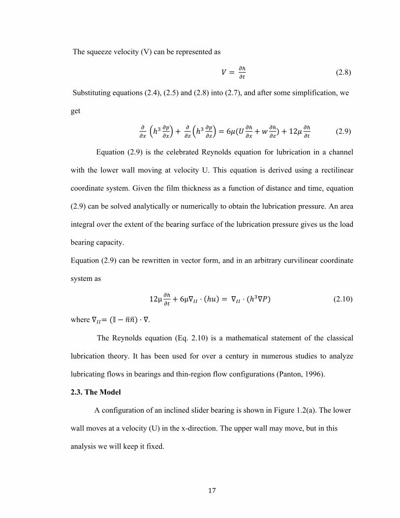
Figure 2.3: Effect of harmonic number on load capacity
surmised from the paper. Yang et al. (2011) chose to represent their results in terms of a
Harmonic Number. Yang et al. (2011) defined harmonic number as the number of
wavelengths per unit (2π) distance. Harmonic number is similar to the wavenumber (k)
defined in section 2.3.
At harmonic number 100, we obtain the same load as Yang et al. (2011), i.e. 10.6
dynes, but at low harmonic numbers we had to use different values of the amplitude
number in order to bring our calculations into agreement with their results. A plot of
bearing load versus harmonic number is shown in Figure 2.3. The dotted line represents
the simulation results at constant amplitude, dashed lines represent the results of Yang et
al. (2011) and the solid line represents the results we obtained at different amplitude
values. Based on the results provided by Yang et al. (2011), the load bearing values are in
good agreement with a systematic error. The small differences in the results can be
attributed to using inaccurate amplitude values. Hence, we can conclude that our
implementation of the surface roughness model is at least the same as an independent
study.

24
2.4.2 Effect of Sinusoidal Surface Roughness on the Load Capacity of a Slider
Bearing
In this section, we analyze the effect of surface roughness, characterized by a
sinusoidal height function of varying amplitude and frequency, on load capacity of slider
bearings. The load capacity is obtained by integrating the lubrication pressure throughout
the entire area of the slider bearing. As discussed in section 2.3, we have cast our results
in terms of roughness number (R) and amplitude number (S). Tables 2.3(a) and 2.3(b)
detail the various parameter spaces we explored.
Table 2.3(a): Table showing amplitude and amplitude number values:
Amplitude (cm) Amplitude number (S) 0.001 0.1 0.002 0.2 0.003 0.3 0.004 0.4 0.005 0.5
Table 2.3(b): Table showing wavelength and roughness number values:
Wavenumber (cm-‐1) Wavelength (cm) Roughness number (R) 10 0.6283 0.02 20 0.3142 0.03 30 0.2094 0.05 40 0.1571 0.06 50 0.1257 0.08 60 0.1047 0.1
An important assumption that we made while deriving the Reynolds’ lubrication
equation is that the variation in the lubrication gap relative to a change in streamwise

25
dimension is small i.e. dh/dx <<1. This assumption limits our parameter space since the
validity of the lubrication approximation deteriorates as dh/dx increases. Figure 2.4 is
pictorial (notional) representation of the “window” in which the lubrication
approximation is valid. It also indicates notionally the relative dimensions of the
roughness variations (amplitude and wavelength) relative to the slider gap to help the
reader interpret the plots. The horizontal axis represents the roughness number (R) and
the vertical axis represents the amplitude number (S). In our problem the quantity dh/dx
can be represented as
!!!"= 𝐴 ∗ 𝑘 cos (𝑘𝑥) (2.18)
Figure 2.4: Lubrication approximation validity “window” along with roughness profiles (not to scale).
Based on the definitions of roughness number and amplitude number (eqn. 2.16),
a roughness number of 1 corresponds to wavelength of 0.01 cm or wavenumber of 628.
dh/dx >> 1 invalid
dh/dx << 1 valid

26
Similarly, an amplitude number of 1 corresponds to amplitude of 0.01 cm. The
lubrication approximation breaks down when dh/dx tends to 1 or when dh/dx > 1. Figure
2.4 gives a good idea on the validity of lubrication approximation with respect to
roughness number and amplitude number. At high S and R, the dh/dx value is much
greater than 1, which implies that the lubrication approximation is no longer valid. At low
S and R, the value of dh/dx is much lesser than 1 and the lubrication approximation is
valid. However, there is a region of uncertainty in between these extremes where the
validity of the lubrication approximation is questionable. In such cases, the validity can
be verified by comparing the results of lubrication approach with a two-dimensional
FEM, full Navier-Stokes model. Good agreement in the results indicates the validity of
the lubrication approximation. Further discussions on computing lubrication window on a
similar exercise of free surface flows can be found in the appendix of this thesis.
In the current problem, the values of roughness number and amplitude number
range from 0.1 to 0.5 and 0.02 to 0.11, respectively. At S = 0.5 and R = 0.11, the values
of amplitude and wavenumber are 0.005 cm and 10 cm-1, respectively. The value of
dh/dx for this particular set of values is 0.35, which is within the lubrication
approximation (dh/dx<<1). We also solve the full Navier-Stokes (NS) equations using
two-dimensional FEM for a range of wavenumbers and compare the results with the
lubrication formulation. Figure 2.5 shows a comparison of lubrication approach and full
NS model. . The simulations were carried out using the following parameters: A = 0.002
cm, L = 6.29 cm, u = 1 cm/s and Hlow = 0.01 cm.
As shown in Figure 2.5, the calculations were performed at four different
wavenumbers i.e. 1, 10, 35 and 70 cm-1. The load capacity values obtained using

27
lubrication formulation are in good agreement with the load values obtained by solving
full Navier-Stokes equations. Hence, we are confident that the lubrication approach is
accurate in this range of parameters, although deviation between the two approaches
begins to become evident for wave numbers greater than 70 cm-1. Also, it is interesting to
note the high load capacity value at wavenumber 1. At wavenumber 1, the slider bearing
can be thought of as an “accelerated” converging-diverging slider bearing. The liquid
flows through a large surface area before it enters the more rapidly converging section
(trough). That is, the curvature of the order of the slider length creates a gap that is
decreasing with distance in higher-order way. The liquid is subjected to very high
pressure in this region due to rapid nonlinear gap convergence thereby generating large
lubrication pressures. This high pressure results in increase of the load capacity.
0 100 200 300 400 500 600 700 800 900
0 10 20 30 40 50 60 70
Load Capacity (dynes)
Wavenumber
Comparsion of load bearing capacity
Lubrication
Full NS
Figure 2.5: Comparison of load capacity for lubrication formulation and full Navier-Stokes solutions.

28
At high wavenumbers, i.e., k > 70, the full Navier-stokes problem required more
than half-million node mesh to resolve the roughness structure whereas the lubrication
formulation needed significantly fewer number of nodes. This clearly shows that the
lubrication approach is more efficient in this range of parameters.
Figure 2.6 shows the effect of velocity on the load capacity. The simulations were
carried out at three different roughness numbers but at a constant amplitude number of
0.003 cm, as shown in the plot. The load capacity increases with increase in roughness
number. With increase in roughness number, the wavelength decreases which results in
higher pressures being generated. This results in a higher load capacity. The relationship
between the load capacity and velocity is linear. This linear dependency of pressure with
velocity can be verified, analytically, by nondimensionalization of the Reynolds equation.
From equation (2.12) in section 2.3, we have
!!"
ℎ! !"!"
= 6𝜇𝑈 !!!"
Integrating the above equation, we get
!"!"= !!"
!! (∆𝐻 + 𝑐) (2.19)
where c is an integration constant.
Upon further integration, equation (2.17) reduces to
∆𝑃 = 6𝜇𝑈.𝛽 (2.20)
where β = (∆!!!)!!
𝑑𝑥

29
Figure 2.6: Effect of wall velocity on load bearing capacity
From equation (2.20), it is evident that the lubrication pressure varies linearly with wall
velocity. Hence, the results in Figure 2.6 are consistent with the expected behavior.
Figure 2.7 shows the effect of amplitude number on load capacity at different
roughness numbers. The dotted line represents the smooth surface. As seen in Figure 2.7,
there is a marginal decrease in the load capacity at low S and low R. In this regime the
gap is large enough for liquid to flow through without much pressure being generated
which results in low load capacity values. In other words, the negative pressures in the
diverging sections of the bearing are more prominent that the positive pressures in the
converging section. This trend reverses with increase in S and R i.e. the positive pressure
regions start to dominate, thereby resulting in higher load capacity values. Also, as R
increases or wavelength decreases, the load capacity increases. At low wavelengths, the
0
5000
10000
15000
20000
25000
30000
35000
40000
45000
50000
0 25 50 75 100
Load Capacity (dynes)
Velocity (cm/s)
Load capacity vs Velocity
R = 0.0318
R = 0.0477
R = 0.0637

30
Figure 2.7: Effect of amplitude number on load bearing capacity
pressure is largely positive since the liquid flow is constricted. This trend is exhibited by
all the curves in Figure 2.7.
Figure 2.8 illustrates the effect of roughness number on the load capacity at
different amplitude numbers. Again, the dotted line represents the ideal case i.e. smooth
surface. As discussed in the previous figure, at low R and S, the load capacity is less as
compared to the smooth case. This is due to the negative pressure regions extending over
a larger portion of the bearing than positive regions, thereby resulting in low load
capacity. As the R and S increase, the gap through which the liquid flows decreases
which in turn results in high pressures being generated. Hence, as R and S increase, the
load capacity gradually increases. Also, it is interesting to note that, at constant
amplitudes, the load capacity curves tend to hit a plateau with increasing R. This is
explained by the diminishing effect of wavelengths on the load capacity.
300
350
400
450
500
550
600
0 0.1 0.2 0.3 0.4 0.5
Load
Cap
acity
(dyn
es)
Amplitude number (S)
Effect of amplitude number on load capacity
Smooth
R = 0.03
R = 0.06
R = 0.11

31
Figure 2.8: Effect of roughness number on load bearing capacity
At high values of R, the wavelengths are so small compared to the gap that their effect on
the load capacity is minimal. This explains the trend exhibited by curves in Figure 2.8.
In short, there are regions of amplitude number and roughness number in figures
2.7 and 2.8 that tend to support much higher load as compared to the smooth surface.
Also, there are specific regions where they tend to support less loads as compared to the
smooth surface. Higher loads are supported when S is greater than 0.2 and R is greater
than 0.06.
200 250 300 350 400 450 500 550 600
0.00 0.02 0.04 0.06 0.08 0.10 0.12
Load Capacity (dynes)
Roughness number (R)
Effect of roughness number on load capacity
Smooth
S = 0.1
S = 0.2
S = 0.3
S = 0.4
S = 0.5

32
CHAPTER 3
Effect of Surface Roughness on the Load Capacity of a Journal Bearing
with Multiphase Flow
3.1 Introduction
Multiphase flow is a term used to describe the simultaneous flow of two or more
fluid phases or components. A two-phase flow system is an example of multiphase flow.
One of the phases is considered to be the primary or continuous phase and the other phase
is considered as the secondary phase and is typically discontinuous, but not always.
Typical examples include oil-water systems, air-water systems, etc.
In general, analyzing the effect of surface roughness on the load capacity of a
journal bearing with extremely narrow gaps relative to the radius and with multiphase
flow is a complex problem due to the extreme geometry, moving interfaces, and resulting
large computational costs involved. There are very few publications on this particular
problem. Cupillard et al. (2008) studied the effect of surface texture on load carrying
capacity and bearing friction of a journal bearing using computational fluid dynamics.
Specifically, they performed an analysis of the effect of deep and shallow dimples.
Dimple position, width and depth were investigated for the deep dimples. They solved
the full Navier-Stokes equations under steady-state conditions with a multiphase
cavitation model. Cupillard et al. (2008) found that textured surface affected the journal
bearing performance.
In this chapter, we also address two-phase flow in a journal bearing but with a
starkly different approach than Cupillard et al. (2008). Specifically, we study the effect of
surface roughness on the load capacity of a journal bearing with two-phase flow using

33
two-phase Reynolds’ lubrication theory, thus addressing the extreme aspect ratio
complexity in a more efficient manner. The surface roughness is characterized by a
sinusoidal wave function.
3.2. Theory
3.2.1 Multiphase Flow
In the preceding chapter, we derived a general form of Reynold’s lubrication
equation (2.10) for a single-phase flow. The same lubrication analysis can be applied to
multiphase flow provided that the fundamental assumptions of lubrication are met.
In our case we will take one fluid as liquid (e.g. water) and the second fluid as a
gas (e.g. air). At the interface, a number of conditions need to be satisfied. First, the
velocities across the interface must be continuous i.e. 𝑢! = 𝑢!. Second, the tensions
need to be balanced; we need to balance the normal traction and tangential traction at the
interface.
We can express this mathematically as follows
𝑃! − 𝑃! + 𝜎∇ ⋅ 𝑛!" = 𝑛!" ⋅ 𝕋𝒂 − 𝕋𝒃 ⋅ 𝑛!" (3.1)
and tangential traction
−∇𝜎 = 𝕋𝒂 − 𝕋𝒃 ⋅ 𝑡!" (3.2)
where 𝜎 is the interfacial tension, ∇.𝑛!" is the total curvature of the interface, 𝑛!" is the
unit vector normal to the fluid interface, and 𝑡!" is the unit vector tangent to the
interface. 𝕋𝒂 is the stress in phase a, and 𝕋!is the stress in phase b. In our model, surface
tension is assumed to be constant which means ∇𝜎 = 0 in (3.2).

34
We use the continuous surface model (CSF) (Brackbill et al. (1992)) to integrate
the interfacial forces into the Reynolds’ lubrication model. A detailed formulation of CSF
can be found in Roberts et al. (2012). The Reynolds’ lubrication equation for multiphase
flow is given by (Roberts et al. 2012):
!(!!)!"
+ ∇!! ⋅!!!𝑈! + 𝑈! − !!
!" ∇!!𝑝 − 𝜎𝜅𝛿 𝜑 𝑛 − 𝑝 𝜑 𝑔 + 𝑓 − 𝑗! + 𝑗! = 0
(3.3)
where κ is the curvature of the interface and p is the lubrication pressure.
The total curvature of the interface, κ, is defined as
𝜅 = −∇.𝑛!" = −∇ ∇!∇!
(3.4)
where F is the level-set function (cf. Section 2.2). However, there are two components of
curvature in the lubrication equation. The z-direction curvature, which is calculated
analytically, and the in-plane curvature, calculated from the level-set field.
The in-plane curvature is calculated as
𝜅!! = −∇!!𝑎𝑛!! = −∇!!𝑎∇!!!∇!!!
(3.5)
where ∇!!= (𝐼 − 𝑛𝑛)∇. Thus, the total curvature is the sum of two components
𝜅 = 𝜅! + 𝑘!! (3.6)
where 𝜅! is the cross gap curvature. It is given by
𝜅! = !!(cos (𝜋 − 𝜃!"#,! − tan!!(𝑛!! ⋅ ∇!!ℎ!)) + cos ( 𝜋 − 𝜃!"#,! − tan!!(−𝑛!! ⋅ ∇!!ℎ!))) (3.7)
Numerical curvature calculations introduce small variations that can lead to
significant changes in the field. This effect becomes more apparent when the length scale
of the problem is small. In order to reduce the effect of such variations, the equation can
35
be mass-lumped and a diffuse term can be added to negate the variations in the curvature
field.
The implemented weak-form of this equation is (Schunk et al. (2011))
𝑅! = 𝜅! ∅!𝑑Ω+ ∇!!!!∇!!!!
.∇!!∅!𝑑Ω+ ℎ!∇!!𝜅!∇!!∅!𝑑Ω (3.8)
where h is the average element size and ∅!is the basis function (cf. Chapter 1). This
equation was implemented in GOMA to be used in conjunction with the shell lubrication
equation. In summary, we will solve three equations to examine multiphase flow in a
journal bearing: the Reynolds’ lubrication equation for lubrication pressure, the level set
equation to track the interfaces, and shell lubrication curvature equation to compute a
more accurate measure of the interface curvature.
3.2.2 Level Set Method
Tracking moving interfaces and coupling the physical properties of different
regions in a domain is a complex problem. Various methods have been proposed over the
years to track interfaces. A standard approach to modeling moving interfaces is based on
discretizing the Lagarangian form of the equations of motion. In this approach, the
parameterization is discretized into a set of marker particles whose position at any time is
used to renormalize the interface front. A few methods that employ this approach are
marker particles methods, string methods and nodal methods (Sethian 1996). In general,
Lagrangian approximations are highly accurate for small-scale motions of interfaces.
However, they suffer from instabilities and geometrical limitations under complex
motions of interfaces as they follow a local representation of the front rather than a global
one.
36
An alternate and efficient approach is an Eulerian formulation. In this approach,
one considers the volume elements at fixed locations in space across through which the
fluid interface flows. The two most commonly used interface tracking methods that
employ an Eulerian formulation are the volume-of-fluid method and level set method.
The level-set approach tracks interfacial evolution through a fixed mesh (Tong
and Wang 2007). For problems in which the interfaces have complex shapes, and for
which large topological shape changes occur (e.g. breakup and coalescence), level-set
embedded tracking is a very efficient and practiced technique. In this method, a specific
level-set value of a level-set field is taken as the interface and is advected in time as a
material surface through a fixed mesh. Advancing the interface as a material surface
tends to distort the rest of the level set field and so that field needs to be constantly
renormalized or reconstructed. This operation can unfortunately lead to a gain or loss of
mass. This is one of the disadvantages of using the level set method.
The level-set equation is based on the assumption that there exists a smooth
function F(x,y), and that it is related to the interface location in space that solves:
𝐹 𝑥,𝑦 = 0 (3.9)
Even though F evolves over time, its zero level contour will always be the
location of the interface. The function F is a smooth function i.e. its gradient in a finite
region around the zero level contour is continuous. This is an important feature because it
implies that the normal vectors to the interface and its curvature are well defined and
readily determined.

37
Evolution of the level set equation is obtained by solving a simple advection equation,
also, known as the kinematic equation:
!" !"+ 𝑢 ⋅ ∇𝐹 = 0 (3.10)
where 𝑢 is velocity field. Solution of the above equation is obtained with the finite
element method on the same mesh as is used for the lubrication formulation. The
Galerkin form of the finite element method deployed by GOMA is known to have issues
with applicability to purely advective equations, but solving/advancing this equation from
an initial smooth datum negates any introduction of dispersion issues. Further discussions
on level set method can be found in Baer et al. (2005).
3.2.3 Implementation in GOMA
The implementation of the level-set algorithm coupled with the lubrication
equations is discussed by Roberts et al. (2012). A distance function F is introduced,
where F = 0 represents the location of the interface between two fluids, say, fluid ‘a’ and
fluid ‘b’. When F < 0, it represents fluid a, and when F > 0 it represents fluid b. The
movement of F is governed by (3.10). For lubrication problems, the level set field is
advected with the mean lubrication field velocity 𝑢 given by
𝑢 = 𝑞ℎ (3.11)
where 𝑞 is the flow rate and h is the lubrication height. In order to implement 3.10 in
GOMA, it is integrated to obtain a residual equation
𝜑! !"!"+ 𝑢.∇!!𝐹 𝑑Ω = 0 (3.12)
where Ω is the computational domain. In order to maintain F as a distance function it
needs to be renormalized. This is done using Huygens method in which a Lagrangian

38
multiplier is used to enforce conservation of the liquid phase before and after
renormalization. Renormalization is done when ∇!!𝐹 is significantly greater than or lesser
than unity at any point of time, based on the specified tolerance.
We can define a unit step function or a Heaviside function H, which is to be evaluated
only at node points. It is a discontinuous function but it can be made continuous by
interpolation using a standard finite element method basis function.
The Heaviside function is given by
𝐻! =0, 𝐹! < 01, 𝐹! > 0 (3.13)
However, we can create a smooth Heaviside function to reduce numerical complications.
Equation (3.13) can be replaced with a smooth Heaviside function given by
𝐻! =
0 𝐹! < 𝛼 !! 1+ !!
!+ sin
(!!!! )
! − 𝛼 ≤ 𝐹! ≤ 𝛼
1 𝐹 > 𝛼
(3.14)
where α is the width of the smooth level set region. Formulation of this smooth,
continuous Heaviside function allows us to express physical properties, such as viscosity
and density, as continuous fields. An exhaustive discussion on using continuum surface
method (CSF) to formulate a flow rate expression using a smooth Heaviside function and
Reynolds’ lubrication implementation can be found in Roberts et al. (2011).
3.3 The Model
A simple journal bearing is illustrated in Fig. 1.2(b). It consists of a journal that
rotates around the bearing surface. The inner shell rotates with an angular velocity ω
while the outer shell remains stationary. Typically, a bearing is filled with a fluid
lubricant that supports the shaft preventing metal-to-metal contact. The most commonly

39
used lubricant is oil. In the case of multiphase flow, the fluids present in the bearing can
be categorized as continuous phase and dispersed phase.
In this problem, we use a two-phase flow system that consists of air as the
continuous phase and water as the dispersed phase. Figure 3.1 illustrates a journal bearing
in which liquid (water) drops are in contact with the journal bearing. The drops are of the
same size. The outer shell of the bearing is characterized by a sinusoidal wave function
and the inner shell is smooth.
The lubricant film thickness h(x) is taken as a sinusoidal function about the mean gap
separation H:
ℎ 𝑥 = 𝐻(𝑥)+ 𝐴. sin (𝑘𝑥) (3.15)
where A is the amplitude of the wave and k is the wavenumber. The mean gap H is
𝐻 𝑥 = 𝐶(1+ 𝜀cos (𝜃) (3.16)
where C is the radial clearance and 𝜀 is the eccentricity.
The wavelength is defined in terms of the wavenumber by:
𝜆 = !!!
(3.17)
The cylindrical solid has a height and radius of 1 cm each, lubrication height H of
0.01 cm, amplitude number S of 0.002 cm. The liquid lubricant density is taken
as 𝜌! = 1 𝑔/𝑐𝑚!, and viscosity as µ = 1 cP. The gas phase viscosity is taken of 0.01 cP.
The density of the liquid and gas are assumed to be equal and constant. The surface
tension used is 70 dyne/cm. Figure 3.1 is a schematic representation of a journal bearing
with liquid drops confined between the walls. The drops are circular in shape with radii 𝑟!
= 0.3 cm each.

40
An important dimensionless parameter that is significant in this problem is the
Capillary number. It is defined as the ratio of viscous forces to surface or interfacial
tension forces, and it is often defined as follows:
𝐶𝑎 = !"!
(3.18)
where µ is the viscosity, 𝜔 is velocity in cm/s and 𝜎 is the interfacial tension. A high
capillary number implies that viscous forces are dominating the interfacial tension forces.
Figure 3.1: Journal bearing: Multiphase flow model with coordinate axes. Liquid (red) drops dispersed in air (blue). Mu represents the viscosity of the phases.

41
The multiphase version of Reynolds lubrication equation is solved along with the
level set equation and shell-lubrication-curvature equation using finite element method in
GOMA. The lubrication load capacity is computed by integration of the pressure acting
on the bearing shaft in x-direction (Fig. 3.1). The results are expressed in terms of load
capacity over a period of time for different values of contact angle, roughness number,
eccentricity and angular velocity.
3.4. Results and Discussions:
Computations were performed for 18 cases with velocity u = 1000 cm/s,
amplitude a = 0.002 cm and lubrication height h = 0.01 cm. Throughout the factor space
of 18 simulations we chose to vary the liquid/gas/solid contact angle, the roughness
number and eccentricity (Figure 1.2(b)). Recall that the roughness number R is defined as
𝑅𝑜𝑢𝑔ℎ𝑛𝑒𝑠𝑠 𝑁𝑢𝑚𝑏𝑒𝑟 𝑅 = !"#$#%& !"#$%&'(%)* !"# (!!"#)!"#$%$&'(!
(3.18)
Figure 3.2 illustrates a phenomenon we encountered in few cases (Fig. 3.4) in our
problem, namely, fingering instability (Chen et al. 1994). Fingering instability occurs at
the interface of two fluids when the less viscous fluid is pushing out a high viscous fluid,
as would be happening when the drop flows through a widening gap. While this
fingering effect is real and a well-known phenomenon, it was undesirable from the
standpoint of computational stability. To pick up the finer scale, free surface features
required smaller mesh size and significantly smaller time step, and often this made the
calculations intractable given the available computer resources.
Due to limitations encountered while performing the simulations we have chosen
to report only fewer results. Figures 3.3 through 3.6 illustrate the effect of surface
roughness on the load capacity as a function of time. Figure 3.3 is a plot of predicted load

42
capacity for three different contact angles i.e. perfect non-wetting (𝜃 = 0 °), neutral
wetting (𝜃 = 90 °) and perfect wetting (𝜃 = 180 °). The oscillatory behavior is due to
the effect of surface roughness (amplitude and wavenumber). Clearly the results show
little dependence of hydrophobicity on the load. In general, one would expect to see a
significant difference in the load capacity between hydrophobic and hydrophilic cases but
this is not the case. The reason for this lack of dependency is that the calculations were
carried out at a high Capillary number.
Figure 3.2: Fingering Instability
In our problem, the capillary number was 14, which clearly is in this regime.
Unfortunately we were unable to carry out calculations at low capillary number, viz. Ca <
1, due to significant mass loss in our calculations. At low capillary number the CSF
approach requires much finer meshes than we could deploy with our limited computer
resources.

43
In figure 3.4, the plot corresponds to simulations performed at an eccentricity of
0.004 cm and a wave number of 10 cm-1. As seen in Figure 3.4, the hydrophilic case tails
off from the other two curves and the calculation failed to complete due to fingering
instability (Figure 3.2).
A quick comparison of figures 3.3 and 3.4 reveals the fact that an eccentric
bearing tend to supports a higher load than the concentric case, which is no surprise but at
least verifies an expected result.
Figure 3.5 is a plot of predicted load capacity for two different contact angles i.e.
perfect non-wetting and perfect wetting. The values of eccentricity and wavenumber for
these two runs were 0.004 cm and 30 cm-1, respectively. Again, because the calculations
were carried out at Ca >>1 we are unable to study wetting effects.
Figure 3.3: Effect of wettability on the load capacity. For these simulations, no eccentricity and wave number = 10 cm-‐1. The three curves correspond to perfect non-‐wetting (𝜃 = 0 °); neutral wetting (𝜃 = 90 °) and perfect wetting (𝜃 = 180 °).

44
Figure 3.5: Effect of wettability on the load capacity. For these simulations, no eccentricity and wave number = 30 cm-1.
Figure 3.4 Effect of wettability on the load capacity. For these simulations, eccentricity = 0.004 cm and wave number = 10 cm-‐1.

45
Figure 3.6: Effect of wettability on the load capacity. For these simulations, eccentricity = 0.004 cm, smooth case. In Figure 3.6, we observe the undesirable result that load capacity decreases over
time due to shrinking drops. We use the level-set renormalization function to reconstruct
the level set function at time steps determined by an error tolerance. This renormalization
process leads to loss of mass and shrinkage of drops. We were not able to resolve the
mass-loss problem and hence chose to show limited results. Nonetheless, we were able
to discern some multiphase flow effects on the journal-bearing load.
In conclusion, the load capacities of all of the three cases i.e. non-wetting, neutral
wetting and perfect wetting in figures 3.3 through 3.6 are quite similar. The capillary
number in these calculations was too high to study the effect of wettability and surface
roughness on the load capacity. We did run a few simulations at a lower speed i.e.
velocity ω = 300 cm/s and hence lower capillary number, but the runs could not be taken
to large enough times before significant mass loss to be conclusive.

46
The goal of the study was to analyze the effect of surface roughness and
wettability on the load capacity of a journal bearing at two different cases i.e. high
volume fraction and low volume fraction of liquid (water) phase. For the high volume
fraction case, we planned on having many small liquid drops spread throughout the
bearing volume i.e. in the range of 75-100 in number. However, when the simulations
were carried out we had several issues. First, the drops started to disappear within a short
period of time due to the level-set renormalization errors that we were not able to
reconcile. Second, the drops began to merge with time due to their close proximity with
each other. Due to these limitations we had to re-structure our problem and eventually,
factor out volume fraction as one of the parameter space for our study.

47
CHAPTER 4
POROUS JOURNAL BEARING
4.1 Introduction
Over the past few decades, porous bearings have received considerable attention
from scientists and engineers. Porous bearings have a wide variety of industrial
applications that include automotive components, household appliances, etc. The major
advantage of porous bearings is that the pores act as a lubricant reservoir thereby
eliminating the need to constantly supply bearings with lubricants. Hence, they are also
known as ‘self-lubricating’ bearings. However, most porous bearings operate under
boundary or mixed lubrication regime (cf. Chapter 1, section 1.2).
Key liquid transport properties in porous media are porosity and permeability.
These properties are set by the microstructure of the medium. Variations in porosity and
permeability exist. These variations can be either natural or deliberate. Several examples
exist in technology wherein such spatial variations are used to create engineering surfaces
or materials. These include nanoimprint lithography, porous absorbent media, and
bearings.
Morgan and Cameron (1957) were the first to study porous bearings with the aid
of hydrodynamic lubrication conditions (Cf. chapter 1, section 1.2.1). Since then, there
have been numerous studies on various porous bearings. Wu (1971) studied squeeze film
porous bearings, Prakash and Vij (194) studied journal bearings, Uma (1977) studied
slider bearings, and Gupta and Kapur (1979) studied thrust bearings. Prakash and Vij
(1974) analyzed the performance of a plane porous slider bearing and found that the
effect of porosity is to decrease the load.

48
In this chapter, we study the effect to porosity and capillary imbibition on the load
capacity of a porous journal bearing. Specifically, we solve the Reynolds’ lubrication
equation along with the porous shell equations (cf. section 4.2) for open, structured
porous media.
4.2. Theory
The laws governing the flow of fluids in porous media are well known. Darcy’s
law is the fundamental equation that describes the flow of fluids through porous media. It
is also the common in various science and engineering fields including civil engineering,
petroleum engineering, geology and chemical engineering. Henry Darcy carried out a set
of experiments in 1855 in order to establish a relation between the volumetric flow rate of
the sand bed and the hydraulic head loss (Simmons 2008). He formed the law based on
the experimental results. The law states that the discharge rate through a porous medium
is proportional to the pressure drop over a distance. The relation is as follows:
𝑄 = !!"!
(!!!!!)!
(4.1)
where Q is the discharge rate, k is the permeability, A is the cross-sectional area of the
flow, µ is the viscosity of fluid, L is the length of the over which the pressure drop (Pb –
Pa ) occurs. A general form of 4.1 is obtained by divided both sides of the equation by A.
𝑞 = !!! ∇𝑃 (4.2)
Here, 𝑞 is the flux and ∇𝑃 is the pressure gradient. The flux 𝑞 is also referred to as the
Darcy flux.
It is given by
𝑣 = !∅ (4.3)

49
where 𝑣 is taken as the velocity of fluid in pores and 𝜙 is the porosity. Equation 4.2 can
also be written as
−∇𝑃 = !!𝑣 (4.4)
𝑣 now becomes a volume-averaged quantity in a porous media.
Porosity is defined as the ratio of volume of free pore space to the total volume of
the material. Pores can be classified as open pores and closed pores. Closed pores are
isolated from each other and when the liquid starts to fill the pores the gas initially
present in the pores is trapped and compressed. In the case of open pores, the pores are
interconnected and when the liquid starts to fill in the pores, the gas is allowed to escape
thereby maintaining its initial pressure. Both these models have been implemented in
GOMA separately (Schunk et al. 2006).
In our study, we will be using an open pore formulation. In this system we
calculate the in-plane velocity from a shell-form of the Darcy equations. In the vertical
direction we use a simpler model, assuming thin shells (Roberts and Schunk, in
preparation).
The vertical pressure gradient is calculated as follows
!"!"=
!!!!!"#!!!!
!" (4.5)
where H is the height of pores, Plub is the lubrication pressure in the gap, r is the pore
radius, S is the saturation level and P0 is the initial gas pressure that remains constant.
The gas pressure is derived from the ideal gas law. The denominator HS comes from the
height that the liquid has penetrated into the pores, which is determined from the

50
saturation. The saturation level (S) is governed by a mass balance:
!"!"= !
∅∇ ⋅− !
!∇𝑃 (4.6)
where S is the saturation level. When S =1 the medium is fully saturated and when S = 0
it is devoid of liquid. The pressure gradients in the planar direction are assumed to arise
from the adjoining lubrication layer
∇!!𝑃 = ∇!!𝑃!"# (4.7)
Equations (4.5), (4.6) and (4.7) are solved for the open pore model by coupling with
lubrication equation (3.3) (Roberts and Schunk, in preparation).
4.3 Model
In our model, we consider a journal bearing geometry with a porous casing.
Figure 4.1 illustrates a porous journal bearing used in our study. The porous casing is
adjacent to the outer casing and the lubricant fills the space between the porous casing
and the inner casing. We analyze the effect of porosity and capillary imbibition on the
Figure 4.1: Schematic of a porous journal bearing

51
load capacity. We vary the porosity (𝜙) and the capillary radius r (cf. eqn. 4.5) while the
other parameters remain unchanged. The lubrication height H is taken as 0.01 cm,
eccentricity as 0.004 cm, velocity as 10 cm/s, liquid density as 1 g/cm3 and liquid
viscosity as 0.01 cP. The pores are initially partially saturated by setting an initial
pressure. The gas present in the pores is considered to be an ideal gas. The open porous
shell equations are solved along with the Reynolds’ lubrication equation in GOMA.
4.4 Results
In this section, we will discuss the effect of porosity and capillary imbibition on
the load capacity. Figure 4.2 is a plot of load capacity in time for different values of
porosity and capillary radii i.e. porosity of 0.3 and 0.8, and capillary radii of 0.01 cm and
0.05 cm.
Figure 4.2: Plot of load capacity for different values of porosity and capillary radii

52
As shown in Fig. 4.2, cases with high porosity i.e. 0.8 takes a longer time to fully
saturate as compared to cases with lower porosity i.e. 0.3. The porosity seems to have a
negative effect on the load capacity for both the cases i.e. capillary radii of 0.01cm and
0.05 cm. A larger load is supported when the porosity is 0.3. It is also interesting to note
that load capacity increases with time, reaches a threshold high and decreases thereafter.
The pressure, initially, is largely negative throughout much of the domain, leading to a
small load. The negative pressure results from capillary suction by the pores, which
outweighs the lubrication pressure. Once the pores start filling, the pressure increases and
tends to go positive. This explains the increase in load capacity. As seen in Fig. 4.2, load
overshoot occurs just before the system becomes fully saturated. A closer investigation of
the lubrication pressure plots and saturation plots reveals a small fluctuation in saturation
levels throughout the bearing. This causes a marginal decrease in pressure that results in
reduction of load capacity. Also, it is interesting to note the oscillatory behavior of the
load in the case of capillary radius r = 0.01 cm. This behavior is due to numerical
artifacts since the lubrication pressure plots didn’t show any indication that could account
for the oscillatory behavior.
In short, bearings with a larger capillary radius tend to support more load than a
smaller radius. However, porosity seems to have an undesirable effect on the load
capacity. Further studies on the effect of porosity on the load capacity should be carried
out to ascertain the claim. It would also be interesting to study the effect of surface
roughness on the load capacity of a porous journal bearing.

53
CHAPTER 5
CONCLUSIONS AND FUTURE WORK
5.1 Conclusion
5.1.1 Slider Bearing Model
In chapter 2, we studied the effect of surface roughness, characterized by a
sinusoidal height function, on load capacity of slider bearings. Finally, a verification
problem was used to verify the accuracy of our sinusoidal surface roughness model.
Our predictions reveal some interesting behavior that might be important for
future studies on slider bearings. We feel that a transient simulation will be required to
analyze further the effect of sinusoidal surface roughness on the load capacity of
bearings.
Nonetheless, the following conclusions can be drawn:
• Surface roughness has significant effects on the slider bearing and its load
capacity, according to the Reynolds lubrication theory.
• Both the wavelength and amplitude have significant impact on the load capacity.
• Specifically, higher loads are supported when S is greater than 0.2 and R is
greater than 0.06.
In the next chapter, we will be using the sinusoidal surface roughness model to study
load capacity in a journal bearing with multiphase flow. Finally, we will study the
more complicated case: surfaces that are solid and porous.

54
5.1.2 Multiphase Flow in Journal Bearing
In chapter 3, we analyzed the effect of surface roughness and multiphase flow on
the load capacity of a journal bearing. We discussed how the Reynolds’ equation can be
modified for two phase flow with interfacial tension, and how the level-set method were
implemented in GOMA.
The following conclusions can be drawn:
• At high capillary numbers, the importance of wetting or contact angle is minimal,
as expected due to viscous forces overwhelming capillary forces.
• In order to carry out a thorough analysis on the effect of surface roughness, the
volume fraction parameter space needs to be explored. The computational cost
involved in such problems will be high due to the requirement of very fine
meshes.
Future work on this topic should include studying the effect of a two-dimensional
surface roughness model and working out an efficient method/way to do high volume
fraction studies by overcoming the limitations encountered, viz. merging and shrinking
drops.
55
APPENDIX
COMPARATIVE STUDY OF COATING FLOWS WITH
CONTINUUM AND LUBRICATION MODELS
1. INTRODUCTION
1.1 COATING FLOW
Continuous liquid film coating is the process of applying a liquid material to a
substrate i.e., the solid surface. The liquid layers that replace gas at the solid surface are
thin and continuous. Coating processes can be broadly categorized into pre-metered and
self-metered coating flows. In self-metered flow, the thickness of the liquid layer is a
function of the process itself. In other words, the web speed, geometry and the liquid
properties determine the thickness of the layer. The most common methods are dip
coating, blade coating and roll coating. In pre-metered coating flow methods, the flow
rate is known and fixed. The liquid properties remain constant throughout and the
thickness is determined. These methods include slot, slide and curtain coating. A
comprehensive discussion on various methods of coating can be found from the Coating
Flows article (Ruschak et al 2004).
Our main focus is on pre-metered slot coating. . Slot-extrusion coating is often
used for higher viscosity liquids. In slot coating, the inlet pressure can be set and the
final thickness is measured. One can also set the inlet flow rate, and coupled with the web
speed the final film thickness is pre-determined. The web speed and liquid properties like
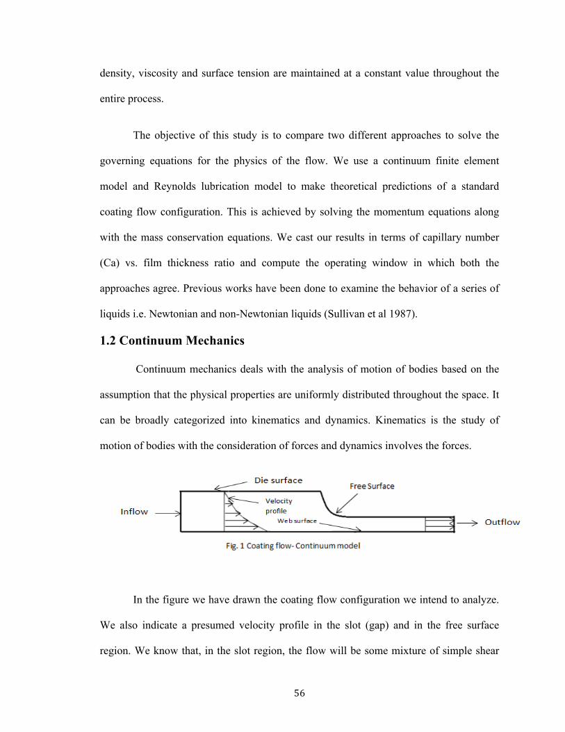
56
density, viscosity and surface tension are maintained at a constant value throughout the
entire process.
The objective of this study is to compare two different approaches to solve the
governing equations for the physics of the flow. We use a continuum finite element
model and Reynolds lubrication model to make theoretical predictions of a standard
coating flow configuration. This is achieved by solving the momentum equations along
with the mass conservation equations. We cast our results in terms of capillary number
(Ca) vs. film thickness ratio and compute the operating window in which both the
approaches agree. Previous works have been done to examine the behavior of a series of
liquids i.e. Newtonian and non-Newtonian liquids (Sullivan et al 1987).
1.2 Continuum Mechanics
Continuum mechanics deals with the analysis of motion of bodies based on the
assumption that the physical properties are uniformly distributed throughout the space. It
can be broadly categorized into kinematics and dynamics. Kinematics is the study of
motion of bodies with the consideration of forces and dynamics involves the forces.
In the figure we have drawn the coating flow configuration we intend to analyze.
We also indicate a presumed velocity profile in the slot (gap) and in the free surface
region. We know that, in the slot region, the flow will be some mixture of simple shear

57
due to the web motion relative to the top die surface and pressure-driven Poiseuille flow.
In the film region the velocity profile will relax to a plug flow, with liquid traveling in
solid body translation with the web. To determine the actual velocity field, we will solve
the Navier-Stokes equations, which can be expressed as
𝜌𝜕𝑢𝜕𝑡 + 𝑢.∇𝑢 = −∇𝑃 + 𝜇∇!𝑢 + 𝑓
∇.𝑢 = 0
In order to solve these equations i.e. the incompressible flow Navier-Stokes
equations, we use the finite element code GOMA (Schunk et al 2009). GOMA is a two-
dimensional and three-dimensional finite element code developed specifically for free
and moving boundary problems. Further details on how these equations were
implemented in GOMA can be found in the GOMA manual (Schunk et al. SAND2006-
5375).
There are instances when the gap width and film region are long and thin in which
it becomes really expensive to solve the Navier-Stokes equations using the full finite
element approach. An alternate approach would be to use the Reynolds lubrication model
which is more efficient in solving problems where the film thickness is small.
We undertake solutions with both methods using finite element code GOMA i.e.
we use the finite element method to solve the full Navier Stokes equations in two
dimensions and also use the Reynolds lubrication to solve for the pressure field and film
thickness.

58
1.3 Reynolds Lubrication
Reynolds lubrication, also known as thin-gap approximation is based on the
assumption that the distance between the boundaries is small as compared to the gap
width. If the boundaries are not parallel, the velocity component varies as a function of
the distance in the flow direction. One can simplify the Navier-Stokes equations by using
a large aspect ratio and neglecting inertial forces i.e. inertial forces are negligible as
compared to the viscous forces.
The governing equations for lubrication theory can be derived from the Navier-
Stokes equation and the continuity equation. The incompressible flow Navier-Stokes
equations in the Vector form, for a liquid with constant density (ρ) and viscosity (µ), can
be written as
𝜌𝜕𝑢𝜕𝑡 + 𝑢.∇𝑢 = −∇𝑃 + 𝜇∇!𝑢 + 𝑓
𝜕𝜌𝜕𝑡 + ∇. 𝜌𝑢 = 0
When the density (ρ) is constant, the second equation reduces to
∇.𝑢 = 0
The Reynolds Lubrication equation derived from the above equations, in its general form,
can be expressed as
12µμ𝜕ℎ𝜕𝑡 + 6µμ∇!! ⋅ ℎ𝑢 = ∇!! ⋅ (ℎ!∇𝑃)
Further details on the equations that GOMA uses to solve can be found in Schunk et al.
(2009).

59
1.3.1 Lubrication Model
The flow region can be separated into two: confined flow and film flow. In the
Confined flow region, the flow is characterized by the Reynolds lubrication. The local
velocity profiles are a combination of a Couette flow and a Poiseuille flow.
The expression for flow rate in this region can be derived using the expression for
velocities given by Couette flow and Poiseuille flow (Panton 1995). It is given by the
following equation:
𝑞 = −ℎ!
12𝜇 ∇𝑃 +𝑈!"#ℎ2
In the film flow region, the flow is no longer confined. The governing equations for the
film flow region can be written as
!!!"+ ∇. !!
!!−∇𝑃 + 𝑈!"#ℎ = 0
In this case, the expression for flow rate is
𝑞 = −ℎ!
3𝜇 ∇𝑃 + 𝑈!"#ℎ
A detailed description on the implementation of these models will be discussed in the
following section.

60
2. The Model
The mesh is generated using the two-dimensional and three-dimensional finite
element mesh generation toolkit CUBIT (GT-001.4). The steps involved in creating a
mesh using CUBIT are geometry creation, interval specifications, meshing and assigning
boundary values (nodesets and sidesets).
The simulations were carried out by varying the inlet pressure and the web speed
over a long range of values. The data were obtained by choosing a particular web speed
and varying the pressure from really low values to high values. The capillary number
(Ca) is the ratio of viscous forces to the surface tension forces. Since the viscosity and the
surface tension are constant throughout, Capillary number is primarily a function of the
web speed.
Automatic continuation technique was used to carry out these simulations in an
easier way. Automatic continuation refers to the set of algorithms that allows us to track
steady-state solution paths as a set of one or more parameters varied. GOMA is currently
capable of zero order, first order, and arc length continuation in a single parameter set,
and bifurcation tracking in two parameter sets (Labreche et al.2006).
2.1 Continuum Model
In fig. 3, the actual model along with various boundary conditions at the surfaces
is shown. The liquid adheres to the top wall and we apply the no-slip boundary condition
(U=0). On the bottom wall, the liquid speed is set equal to the web speed (U=Uweb). The
velocity in the y-direction (v) is zero on the boundaries. The kinematic boundary
condition is applied at the free surface i.e. the liquid velocity perpendicular to the solid

61
surface vanishes on the boundary itself (n.U = 0). These boundary conditions along with
the Navier-Stokes equations are solved using the GOMA.
At low web speed and low pressure values, we expect the meniscus to be concave, shown
in fig. 3, and at high web speeds and high pressures, we expect the meniscus to be
convex.
2.2 Lubrication Model
The governing equations for the confined flow region and the film flow region are
solved along with the boundary conditions as described in fig. 4. The governing
equations for the confined flow region and film flow region are
Confined flow:
12µμ𝜕ℎ𝜕𝑡 + 6µμ∇!! ⋅ ℎ𝑢 = ∇!! ⋅ (ℎ!∇𝑃)
Film flow:
!!!"+ ∇. !!
!!−∇𝑃 + 𝑈!"#ℎ = 0
Fig. 3 Two-‐dimensional Continuum model with the boundary conditions
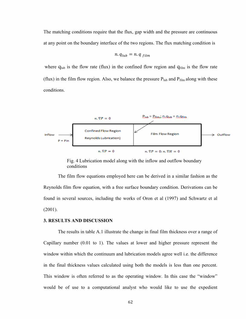
62
The matching conditions require that the flux, gap width and the pressure are continuous
at any point on the boundary interface of the two regions. The flux matching condition is
𝑛. 𝑞!"# = 𝑛. 𝑞 !"#$
where qlub is the flow rate (flux) in the confined flow region and qfilm is the flow rate
(flux) in the film flow region. Also, we balance the pressure Plub and Pfilm along with these
conditions.
The film flow equations employed here can be derived in a similar fashion as the
Reynolds film flow equation, with a free surface boundary condition. Derivations can be
found in several sources, including the works of Oron et al (1997) and Schwartz et al
(2001).
3. RESULTS AND DISCUSSION
The results in table A.1 illustrate the change in final film thickness over a range of
Capillary number (0.01 to 1). The values at lower and higher pressure represent the
window within which the continuum and lubrication models agree well i.e. the difference
in the final thickness values calculated using both the models is less than one percent.
This window is often referred to as the operating window. In this case the “window”
would be of use to a computational analyst who would like to use the expedient
Fig. 4 Lubrication model along with the inflow and outflow boundary conditions

63
lubrication approach and would like to keep within a region of parameter space with
minimal error. Here, we refer to it as the lubrication operating window.
A plot between the capillary number and the film thickness ratio is shown in fig.
5. For free surface flows the most important dimensionless parameter is the capillary
number (Ca).The capillary number is the ratio of viscous forces to surface tension forces.
We define it as
𝐶𝑎 = 𝜇.𝑈!"#𝜎
At really low web speed and high pressure, the film thickness ratio is as high as
15. Such a high value for the thickness ratio can be accounted by the fact that at low web
speeds, the web moves too slowly relative to the inlet flow rate to draw the film down, as
Web
speed
(Uweb)
Capillary
number
(Ca)
Low
Pressure
(Plow)
Final
film
thickness
at Plow
(hlow)
High
Pressure
(Phigh)
Final film
thickness at
Phigh(hhigh)
Film
thickness
ratio
(Hlow =
hlow/hgap)
Film
thickness
ratio
(Hhigh=
hhigh/hgap)
0.1 0.01 -1.97E+4 20.88 8.70E+5 1478.91 0.2088 14.7891
0.5 0.07 -7.70E+4 25.91 2.50E+6 872.94 0.2591 8.7294
1 0.14 -1.35E+5 28.57 4.00E+6 708.56 0.2857 7.0856
4 0.57 -4.80E+5 30.64 1.20E+7 543.89 0.3064 5.4389
7 1 -8.10E+5 31.28 1.90E+7 496.98 0.3128 4.9698
Table A.1: Film thickness ratios computed at different web speeds and pressures.

64
a result of which the final film thickness is much greater than the slot gap. The capillary
number in this case is small, indicating that surface tension forces are dominant. Also, at
low web speeds, we inferred that the distance or the length needed for the thickness of the
boundary layer to evolve is much more than the length needed at high web speeds. Thus,
the length of the free surface was varied depending on the web speed. The length was set
to, as high as, 3 cms at low web speeds and 1 cm at high web speeds.
It is interesting to note that, from fig. 5, the change in film thickness ratio is
minimal at low pressures. This pattern could suggest that the web speed is not the only
parameter that could affect the final thickness. When the pressure is really low or even
negative, backflow is induced in the system thereby reducing the film thickness and
causing the meniscus to be concave.
The free surface shapes as indicated by the mesh pattern, for continuum model, in
fig. 6 correspond to the points A, B, C and D on the plot in fig. 5, respectively. As
expected, the meniscus is concave at low web speeds and low pressures (Fig 6 (A) and 6
(c)) and at high web speeds, high pressures the meniscus is convex (Fig 6(B) and 6(D)).

65
4. CONCLUSION
The lubrication-operating window has been computed and the theoretical
predictions have been discussed. Future works on computing the operating window for
coating flow can be based on this work. Experiments can be carried out to verify the
theoretical predictions made here. Comparison of theoretical predictions and
experimental values would certainly give us a good qualitative analysis. It will be
interesting to implement these models to study the rheological phenomena of various
liquids and look at how the operating window differs for different liquids.

66
REFERENCES
Baer, T.A., and Schunk, P.R. (2005). Tutorial on Level Set tracking in GOMA. GT-
020.3. Sandia Report.
Batchelor, A.W., and Stachowiak G.W.(2000). Engineering Tribology (2nd ed.).
Butterworth-Heinemann.
Boschkova K. (2002). Adsorption and frictional properties of surfactant assemblies at
solid surfaces. KTH, Sweden.
Brackbill, J.U., Kothe, D.B., and Zemach, Z. (1992). A continuum method for modeling
surface tension. Journal of Computational Physics 100. 335-354.
Burton, R. (1963). Effect of two-dimensional sinusoidal roughness on the load support
characteristics of a lubricant film. Journal of Basic Engineering Transactions ASME, 85,
258-264.
Christensen, H. and Tonder, K.C. (1969), “Tribology of rough surface: Stochastic models
of hydrodynamic lubrication”, SINTEF, Report No. 10/69-18.
Cupillard, S., Cervantes, M.J., and Glavatskih, S. (2008). A CFD Study of a finite
textured journal bearing. Journal of engineering tribology. Part J.222 (97).
Dowson, D. (1998). History of Tribology (2 ed.): Wiley.
Elrod, H. (1979). A general theory for laminar lubrication with Reynolds roughness.
Trans. ASME J. Lubr. Technol., 101(1), 8-14.
Gartling, D.K., Reddy, J.N. (2000). The Finite Element Method in Heat Transfer and
Fluid Dynamics. Second Edition. CRC Press.
Guha, S. (1993). Analysis of dynamic characteristics of hydrodynamic journal bearing
with isotropic roughness effect. Wear, 167, 301.
67
Gupta, J., & Deheri, G. (1996). Effects of roughness on the behavior of squeeze film in a
spherical bearing. Tribology Transactions, 39, 99-102.
Gupta, R.S., Kapur, V.K. (1979), "Centrifugal effects in hydrostatic porous thrust
bearing", Journal of Lubrication Technology, Vol. 101 pp.381.
Hamrock, B.J., Scmid, R.S., and Jacobson, B.O. (2004). Fundamentals of Fluid Flim
Lubrication. CRC Press.
Hori, Y. (2006). Hydrodynamic Lubrication. Tokyo: Springer.
Jost, P. (1966). Lubrication (tribology) - A Report on the Present Position and Industry's
Needs (D. o. E. a. Science, Trans.). HMSO.
Kuzmin, L. (2010). Interfacial Kinetic Ski Friction. (PhD), Mid Sweden University,
Ostersund, Sweden.
Labreche D.A., Wilkes E.D, Hopkins M.M., and Sun A.C. (2006). Advanced Capabilities
in GOMA 5.0 - Augmenting Conditions, Automatic Continuation and Linear Stability
Analysis. Sandia National Laboratories Technical Report. SAND2006-7304.
Morgan, V.T., Cameron, A. (1957), "Mechanism of lubrication in porous metal
bearings", Proc. Conf. on Lubrication and Wear, Institution of Mechanical Engineers,
London, pp.151-7.
Oron A, Davis S.H., and Bankoff S.G. (1997). Long-scale evolution of thin liquid films.
Reviews of Modern Physics. 69.
Panton, R.L., (1996). Incompressible Flow. Second Edition. John Wiley & Sons, Inc.
Patir, N., & Cheng, H. (1978). An average flow model for determining effects of three
dimensional roughness on partial hydrodynamic lubrication. ASME J. Lubr. Technol,
100(1), 12-17.

68
Prakash, J., Vij, S.K. (1974), "Analysis of narrow porous journal bearing using Beavers-
Joseph Criteria of velocity slip", Journal of Applied Mechanics, Vol. 41 pp.348-54.
Reynolds, O. (1886). On the Theory of Lubrication and Its Application to Mr.
Beauchamp Tower's Experiments, Including an Experimental Determination of the
Viscosity of Olive Oil. Philosophical Transactions of the Royal Society of London, 177,
157-234.
Roberts, S.A., Noble, D.R., Schunk, P.R., & Benner, E.M. (2011). Multiphase
hydrodynamic lubrication flow using a three-dimensional shell finite element model,
Submitted.
Ruschak K.J., and Weinstein S.J. (2004). Coating Flows. Annual Rev. Fluid Mech.
36.29–53.
Schunk P.R., and Labreche D.A. (2002). GOMA and SEAMS tutorial, Sandia National
Laboratories Technical Report. GT-001.4.
Schunk P.R., Sackinger P.A., Rao R.R., Secor R.B. (2006). GOMA 5.0 – A Full-Newton
Finite Element Program for Free and Moving Boundary Problems with Coupled
Fluid/Solid Momentum, Energy, Mass and Chemical Species Transport: User’s
Guide.SAND2006-5375.
Schunk, P.R., Secor, R., Tjiptowidjojo, K., and Roberts, S.A. (2011). Thin-shell
lubrication capability in GOMA. Sandia Report.
Schwartz L. W., Roy R.V, Eley R.R., and Petrash S. (2001). Dewetting Patterns in a
Drying Liquid Film. Journal of Colloid and Interface Science 234. 363–374.
Seireg, A. A. (1998). Friction and Lubrication in Mechanical Design: CRC Press.
Sethian, J.A. (1996). Level Set Methods. Cambridge University Press.

69
Simmons, C.T. (2008). “Henry Darcy (1803–1858): Immortalised by his scientific
legacy”. Hydrogeology Journal. 16, 1023-1038.
Stribeck, R. (1902). Die wesentlichen Eigenschaften der Gleitund Rollenlager—the key
qualities of sliding and roller bearings. Zeitschrift des Vereines Deutscher Ingenieure,
46(38,39), 1342-1348, 1463-1470.
Sullivan T., and Middleman S. (1987). Use of a Finite-Element Method to Interpret
Rheological Effects in Blade Coating. AICHE Journal. 33, 70.
Tonder, K. (1996). Dynamics of Rough Slider Bearings: Effects of One-sided
Roughness/Waviness. Tribology International, 29(2), 117-122.
Tong, A.Y, and Wang, Z. (2007). A numerical method for capillarity-dominant free
surface flows. Journal of Computational Physics. 221. 506-523.
Tzeng, S., & Saibel, E. (1967). Surface Roughness Effect on Slider Bearing Lubrication.
A S L E Transactions, 10(3), 334-348.
Uma, S. (1977), "The analysis of double-layered porous slider bearing", Wear, Vol. 42
pp.205-15.
Wilcock, D. F. (1950). Turbulence in High-Speed Journal Bearings. Transactions of
ASME, 72, 825-834.
Wu, H. (1971), "An analysis of the squeeze film between porous rectangular plates",
Journal of Lubrication Technology, Paper No. 71-Lub-2.
Yang, J., Zhang, F., Liu, J., and Zhou, J. (2011). Load-Carrying Capacity Analysis for
Sinusoidal Surfaces Hydrodynamic Bearing. Advanced Materials Research, 295-297,
1244-1250.