flow distortion in non-orthogonal 3- d sonic anemometers t.w. horst, s.p. oncley, and s.r. semmer...
TRANSCRIPT

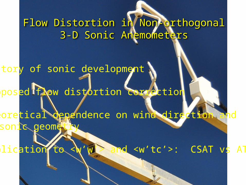
Flow Distortion in Non-orthogonal 3-D Sonic Anemometers
T.W. Horst, S.P. Oncley, and S.R. Semmer
National Center for Atmospheric Research
Boulder, CO
Flow Distortion in Non-orthogonal 3-D Sonic Anemometers
• History of sonic development
• Proposed flow distortion correction
• Theoretical dependence on wind direction and sonic geometry
• Application to <w’w’> and <w’tc’>: CSAT vs ATI-K:


Chandran Kaimal
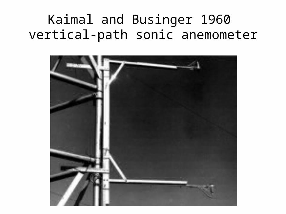
Kaimal and Businger 1960 vertical-path sonic anemometer
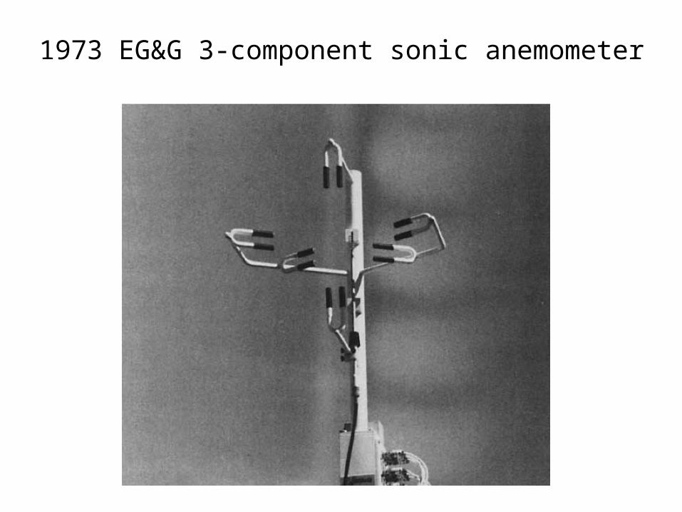
1973 EG&G 3-component sonic anemometer

Transducer Shadowing (Zhang et al, 1986)

Transducer shadowing depends on wind direction w.r.t. path and L/d (Kaimal, 1979)
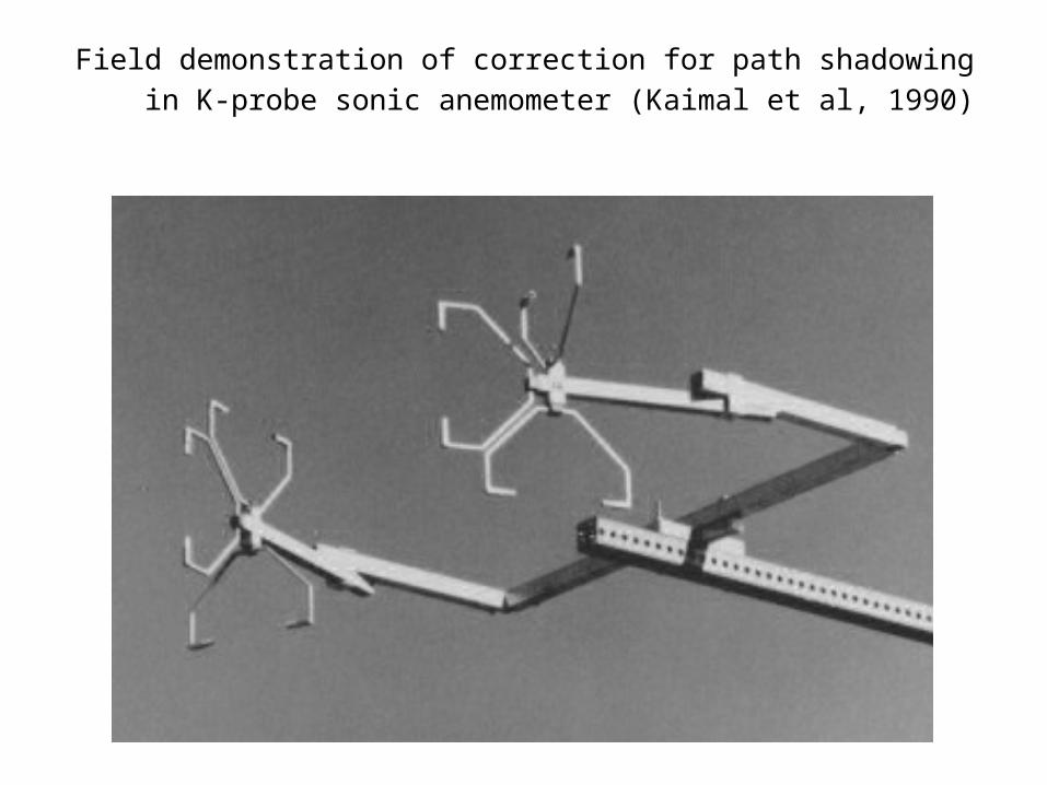
Field demonstration of correction for path shadowing in K-probe sonic anemometer (Kaimal et al, 1990)

Kaimal, Gaynor, Zimmerman and Zimmerman, 1990
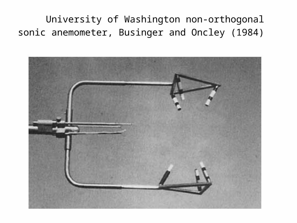
University of Washington non-orthogonal sonic anemometer, Businger and Oncley (1984)

Gill non-orthogonal sonic anemometer

Vertical velocity statistics, such as <w’w’> and <w’Ts’>, are measured to be less with a non-orthogonal sonic than with a vertical-path sonic.

CSAT Transducer Shadowing, L/d = 18, d/L = 0.056
+18


u,v,w,tc from HATS data Sept 2, 2000

Simulation of transducer shadowing
• Transform observed uvw data to path wind components abc
• Apply transducer shadowing to abc, e.g. a_attenuated = a [0.84 + 0.16 sin(theta_a)]• Transform attenuated path components back to
orthogonal coordinates uvw_attenuated• Compare attenuated uvw statistics to original data

Simulation of transducer shadowing
• Transform observed uvw data to path wind components abc
• Apply transducer shadowing to each path, e.g. a_attenuated = a [0.84 + 0.16 sin(theta_a)]• Transform attenuated path components back to
orthogonal coordinates uvw_attenuated• Compare attenuated uvw statistics to original data

Simulation of transducer shadowing

Simulated attenuation by transducer shadowing

Marshall-2012 sonic anemometer field test
CSAT.x(reference)
CSAT.va(vertical a-path)
ATI-K.e(reference)
CSAT.w (reference)
5 sonics at 3m height, 0.5 m spacing
ATI-K.w(reference)


Can coherent continuous-wave Doppler Lidars beutilized for in-situ instrument calibration?E. Dellwik, J. Mann, N. Angelou, E. Simley,
M. Sjoholm & T. Mikkelsen, Technical University of DenmarkJanuary 2014 – ISARS, New Zealand
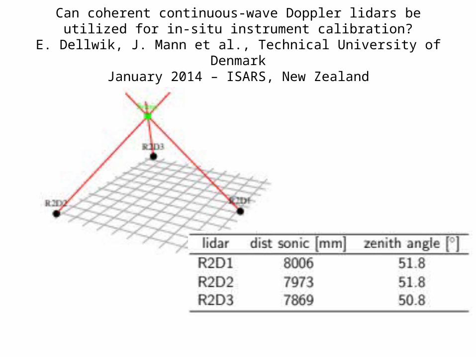
Can coherent continuous-wave Doppler lidars beutilized for in-situ instrument calibration?
E. Dellwik, J. Mann et al., Technical University of DenmarkJanuary 2014 – ISARS, New Zealand

Lidar 0.8 m ahead of sonic
Lidar co-located with sonicu, v, w: fine lines, sonic; broad lines, Lidar (60 Hz data)