Computational Fluid Dynamics using Ansys Fluent (ver. 14.5.7)

Flow Characteristics of the Dyson Air Multiplier

December 7, 2014University of Southern Denmark, Technical Faculty, ITI

Lasse C. ManssonB.Sc. Physics & Technology

&Simon H. Traberg-LarsenB.Sc. Physics & Technology

Abstract

In this CFD report, the fluid physics of the Dyson Air Multiplier is simulated usingAnsys Fluent (ver. 14.5.7). The purpose of the simulation is to demonstrate the governingair flow phenomena inducement, enstrainment, and air loop amplification, and to study thetheoretical performance characteristics of the Dyson Air Multiplier. The model parametersused in the simulation are based on an acquired real copy of the product, which gives riseto not only qualitative, but also quantitative comparisons between the simulated and thereal performance. In the industry, this kind of prototype-simulation coupling is termedSDPD (simulation driven product development) and can greatly reduce costly investmentsand speed up the R&D phase of product development.

Keywords: CFD, inducement, enstrainment, air multiplication, loop amplification,SDPD.

1 Introduction and motivation

The Dyson Air Multiplier (depicted in figure 1.1) is a ventilating fan with no external blades.It consists of a cylindrical base stand, in which the electric motor and internal blades draw inair. The base supports an approx. 30 cm diameter hollow airfoil-shaped ring with a 1.3 mmnarrow slit (jet nozzle).

Figure 1.1: Product image of Dyson Air Multiplier. Dimensions: height × width × depth: 50 cm × 30.5 cm× 9.9 cm. Right image shows detailed view of airfoil shape with narrow nozzle for jet generation.

Dyson claims that the suction system in the base stand can produce an input air flow of20 litres per second[1], meaning a velocity of approximately 1.2 m/s considering the cross-sectional area of the base. The air is then forced through the inner volume of the hollow airfoilring. In order for the fan to effectively ”multiply” (amplify) the air flow, it needs to drawin air from behind the fan. This suction, also called inducement, is obtained by acceleratingthe input air flow by use of the narrow jet nozzle and a loop amplifier1 so that the air isrushed over the airfoil. This generates a low pressure in the the volume encapsulated by the

1Mechanical curvature that accelerates fluid motion

1

airfoil ring that sucks in the air from behind the fan. Actual measurements show that thevelocity of the jet of air at the nozzle is approx. 24 m/s[3]. This fact is used as a validationreference in the forthcoming simulations. In addition, air surrounding the cylindrical outputflow produced by the fan is accelerated and carried along due to viscous shearing. This effectis also termed enstrainment. The total air flow amplification is claimed to be approx. 15times[4], mimicking the output flow of a traditional fan.

The purpose of this report is to study the flow characteristics of the Air Multiplier. E.g.where does turbulence arise, and to what extend? Turbulence is a known source of acousticnoise problems, and is thus desired to be minimized. Depending on the flow type, severalappropriate simulation models exist (e.g. k − ε, k − ω, laminar). This report gives a briefoverview of the significant differences in the results when changing between these models.The actual functionality of the Air Multiplier is a combination of the reach of the fan andthe magnitude of the flow that it can produce. Thus, by use of simulations, the reach andthe center-axis air velocity (at maximal inlet air velocity) are estimated and compared toempirical observations2. The near-field/far-field characteristics of the fan are briefly studied,and so are the effects of inducement and enstrainment.

In the industry, this kind of SDPD (simulation driven product development) is a prototype-simulation-prototype iteration approach to product development. This can in many cases re-duce costly research investments and increase vital knowledge about the working physics[2],[5].

2 Simulation methods

The geometry for simulating the Dyson Air Multiplier is the airfoil-shaped ring, that is shownin the left of figure 2.1, and the base cylinder is not taken into account.The ring is created from an airfoil-shaped 2D sketch that is also shown in the left of figure2.1. This 2D sketch is then revolved 360◦ with respect to a center axis (17.5 cm offset in they-direction) in order to get the shape of a ring. The narrow jet nozzle and the flow inlet canbe seen in the figure. All the other sides and edges in the geometry are defined as no-slipwalls.

Figure 2.1: 3D geometries in the upper part and 2D geometries in the lower part. Left: Geometries withoutmesh. Right: Geometries with mesh.

2Accurate measurement equipment are not available, so results throughout the paper are rough estimates.

2

The right side of figure 2.1 shows the 3D and 2D geometries including mesh. The mesh isa mix of tetrahedrals and quadrilaterals, and in the far-field of the fan the mesh is structuredby using Mapped Face Meshing. The resolution of the mesh is higher close to the fan due tothe relatively small dimensions, and since turbulence is expected here3.

When simulating the flow from the fan, air is used as the medium, where ρ = 1.225 kg/m3

and µ = 1.7894 · 10−5 kg/ms are density and dynamic viscosity, respectively.For solution initialization, the standard initialization method is used together with the

default settings, and the initialization is done by using initial values from the inlet. Velocitiesin x, y and z directions are defined as -2, 0 and 0 m/s, respectively, in correspondence withempirical results (the jet speed has to be approx. 24 m/s).k− ε and k−ω models are used as turbulent viscous models, and their Turbulent DissipationRates are 0.1386289 s−1 and 102.688 s−1, respectively. In both of the models the TurbulentKinetic Energy is 0.015 m2/s2.

The boundaries of the simulation are defined by a box with symmetry boundary conditions.Other boundary conditions such as pressure outlet and wall have been studied, but the mostreliable results (compared to reality) are obtained with the symmetry conditions.The criteria of convergence is defined as 10−3 for all simulation variables.

3 Simulation results

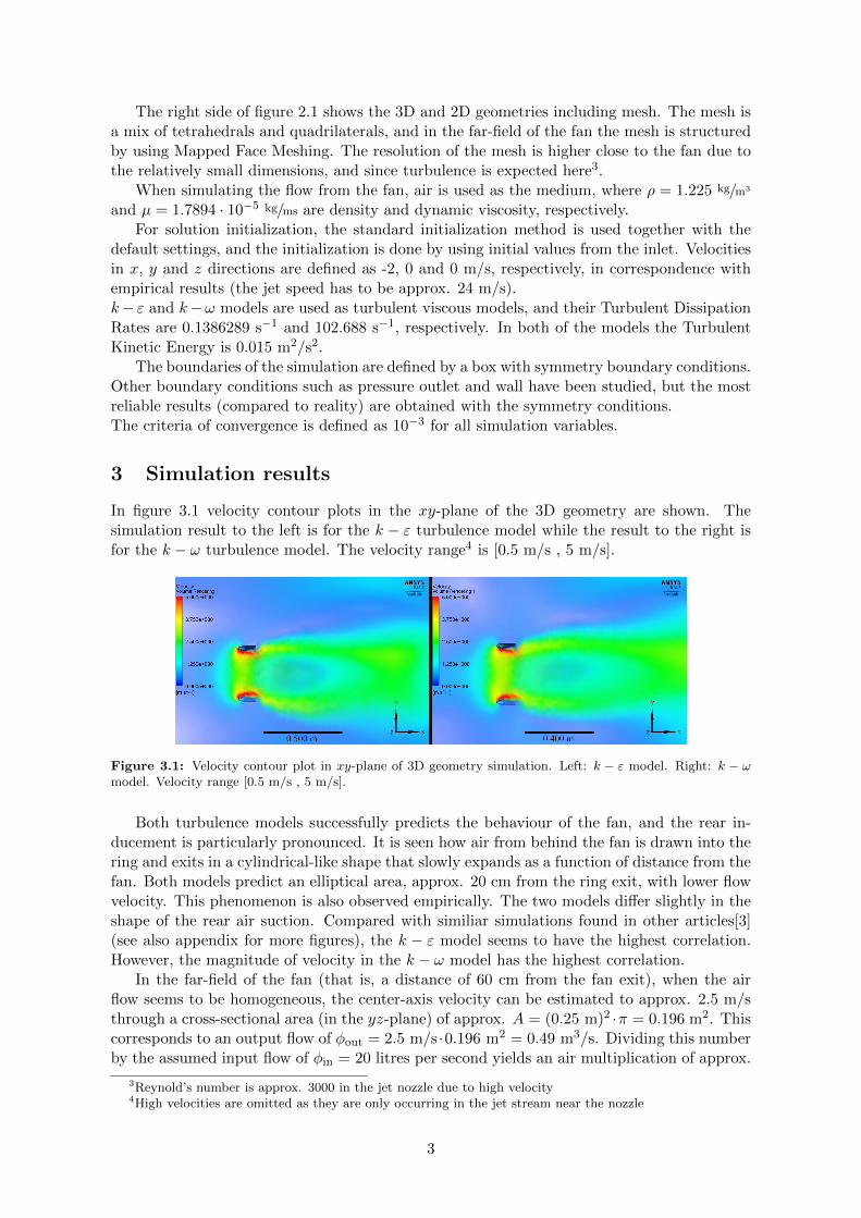
In figure 3.1 velocity contour plots in the xy-plane of the 3D geometry are shown. Thesimulation result to the left is for the k − ε turbulence model while the result to the right isfor the k − ω turbulence model. The velocity range4 is [0.5 m/s , 5 m/s].

Figure 3.1: Velocity contour plot in xy-plane of 3D geometry simulation. Left: k − ε model. Right: k − ωmodel. Velocity range [0.5 m/s , 5 m/s].

Both turbulence models successfully predicts the behaviour of the fan, and the rear in-ducement is particularly pronounced. It is seen how air from behind the fan is drawn into thering and exits in a cylindrical-like shape that slowly expands as a function of distance from thefan. Both models predict an elliptical area, approx. 20 cm from the ring exit, with lower flowvelocity. This phenomenon is also observed empirically. The two models differ slightly in theshape of the rear air suction. Compared with similiar simulations found in other articles[3](see also appendix for more figures), the k − ε model seems to have the highest correlation.However, the magnitude of velocity in the k − ω model has the highest correlation.

In the far-field of the fan (that is, a distance of 60 cm from the fan exit), when the airflow seems to be homogeneous, the center-axis velocity can be estimated to approx. 2.5 m/sthrough a cross-sectional area (in the yz-plane) of approx. A = (0.25 m)2 ·π = 0.196 m2. Thiscorresponds to an output flow of φout = 2.5 m/s ·0.196 m2 = 0.49 m3/s. Dividing this numberby the assumed input flow of φin = 20 litres per second yields an air multiplication of approx.

3Reynold’s number is approx. 3000 in the jet nozzle due to high velocity4High velocities are omitted as they are only occurring in the jet stream near the nozzle

3

24, which is higher than the claimed value of 15 from Dyson[4]. However, it is not knownhow Dyson calculates their air flow amplification, and the errors in the above simulations areunknown as well.

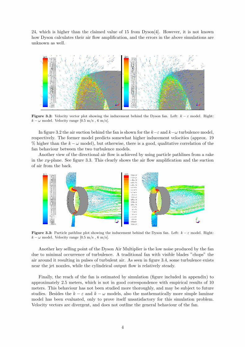
Figure 3.2: Velocity vector plot showing the inducement behind the Dyson fan. Left: k − ε model. Right:k − ω model. Velocity range [0.5 m/s , 6 m/s].

In figure 3.2 the air suction behind the fan is shown for the k−ε and k−ω turbulence model,respectively. The former model predicts somewhat higher inducement velocities (approx. 19% higher than the k−ω model), but otherwise, there is a good, qualitative correlation of thefan behaviour between the two turbulence models.

Another view of the directional air flow is achieved by using particle pathlines from a rakein the xy-plane. See figure 3.3. This clearly shows the air flow amplification and the suctionof air from the back.

Figure 3.3: Particle pathline plot showing the inducement behind the Dyson fan. Left: k − ε model. Right:k − ω model. Velocity range [0.5 m/s , 6 m/s].

Another key selling point of the Dyson Air Multiplier is the low noise produced by the fandue to minimal occurrence of turbulence. A traditional fan with visible blades ”chops” theair around it resulting in pulses of turbulent air. As seen in figure 3.4, some turbulence existsnear the jet nozzles, while the cylindrical output flow is relatively steady.

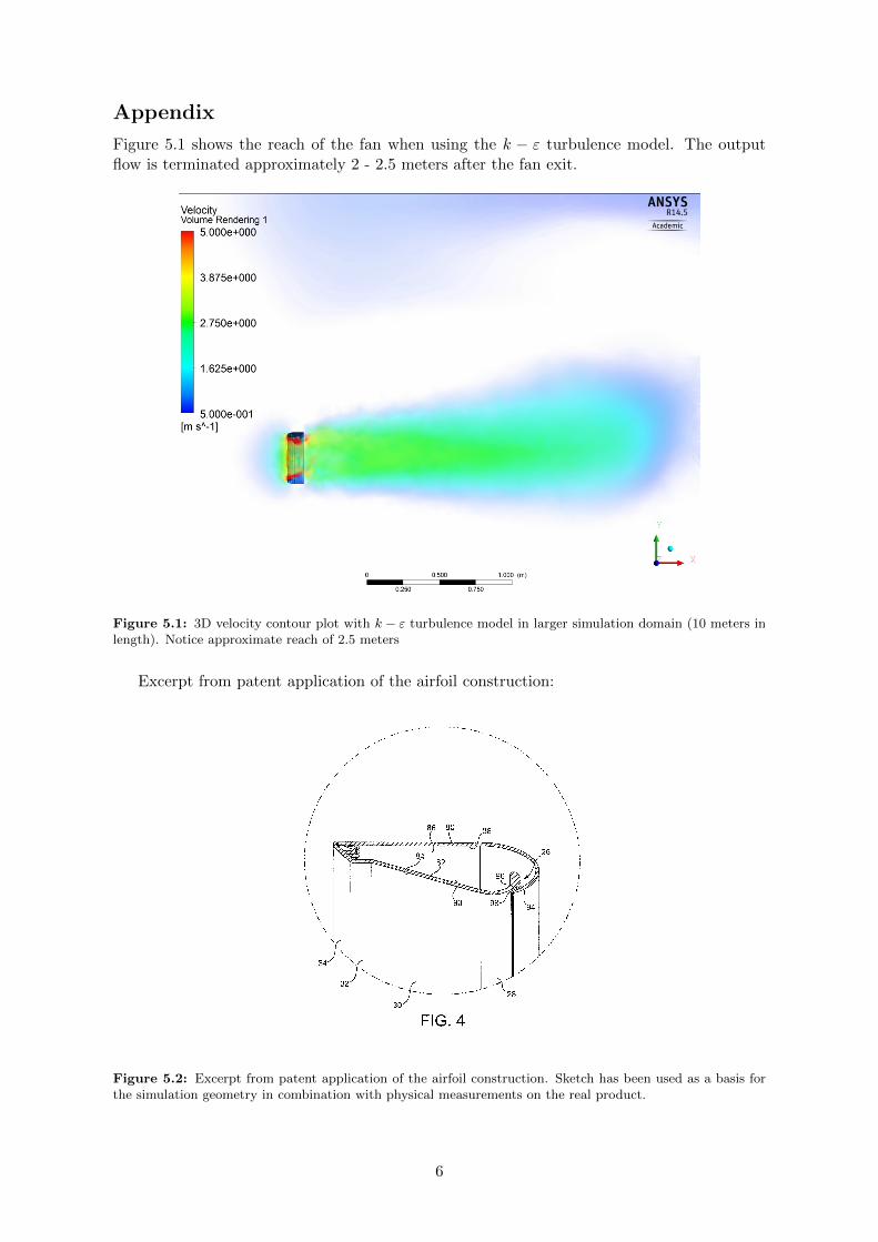
Finally, the reach of the fan is estimated by simulation (figure included in appendix) toapproximately 2.5 meters, which is not in good correspondence with empirical results of 10meters. This behaviour has not been studied more thoroughly, and may be subject to futurestudies. Besides the k − ε and k − ω models, also the mathematically more simple laminarmodel has been evaluated, only to prove itself unsatisfactory for this simulation problem.Velocity vectors are divergent, and does not outline the general behaviour of the fan.

4

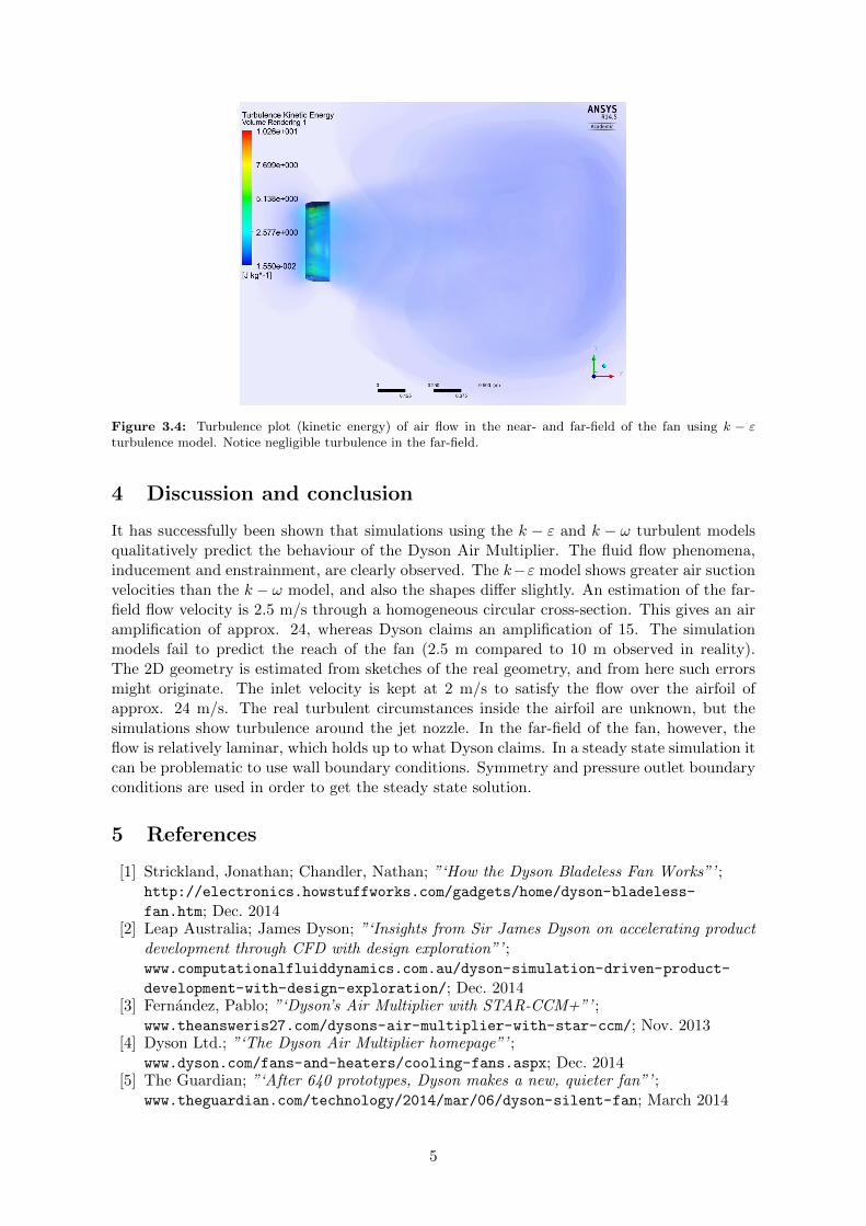
Figure 3.4: Turbulence plot (kinetic energy) of air flow in the near- and far-field of the fan using k − εturbulence model. Notice negligible turbulence in the far-field.

4 Discussion and conclusion

It has successfully been shown that simulations using the k − ε and k − ω turbulent modelsqualitatively predict the behaviour of the Dyson Air Multiplier. The fluid flow phenomena,inducement and enstrainment, are clearly observed. The k−ε model shows greater air suctionvelocities than the k − ω model, and also the shapes differ slightly. An estimation of the far-field flow velocity is 2.5 m/s through a homogeneous circular cross-section. This gives an airamplification of approx. 24, whereas Dyson claims an amplification of 15. The simulationmodels fail to predict the reach of the fan (2.5 m compared to 10 m observed in reality).The 2D geometry is estimated from sketches of the real geometry, and from here such errorsmight originate. The inlet velocity is kept at 2 m/s to satisfy the flow over the airfoil ofapprox. 24 m/s. The real turbulent circumstances inside the airfoil are unknown, but thesimulations show turbulence around the jet nozzle. In the far-field of the fan, however, theflow is relatively laminar, which holds up to what Dyson claims. In a steady state simulation itcan be problematic to use wall boundary conditions. Symmetry and pressure outlet boundaryconditions are used in order to get the steady state solution.

5 References

[1] Strickland, Jonathan; Chandler, Nathan; ”‘How the Dyson Bladeless Fan Works”’ ;http://electronics.howstuffworks.com/gadgets/home/dyson-bladeless-

fan.htm; Dec. 2014[2] Leap Australia; James Dyson; ”‘Insights from Sir James Dyson on accelerating product

development through CFD with design exploration”’ ;www.computationalfluiddynamics.com.au/dyson-simulation-driven-product-

development-with-design-exploration/; Dec. 2014[3] Fernandez, Pablo; ”‘Dyson’s Air Multiplier with STAR-CCM+”’ ;

www.theansweris27.com/dysons-air-multiplier-with-star-ccm/; Nov. 2013[4] Dyson Ltd.; ”‘The Dyson Air Multiplier homepage”’ ;

www.dyson.com/fans-and-heaters/cooling-fans.aspx; Dec. 2014[5] The Guardian; ”‘After 640 prototypes, Dyson makes a new, quieter fan”’ ;

www.theguardian.com/technology/2014/mar/06/dyson-silent-fan; March 2014

5

Appendix

Figure 5.1 shows the reach of the fan when using the k − ε turbulence model. The outputflow is terminated approximately 2 - 2.5 meters after the fan exit.

Figure 5.1: 3D velocity contour plot with k − ε turbulence model in larger simulation domain (10 meters inlength). Notice approximate reach of 2.5 meters

Excerpt from patent application of the airfoil construction:

Figure 5.2: Excerpt from patent application of the airfoil construction. Sketch has been used as a basis forthe simulation geometry in combination with physical measurements on the real product.

6

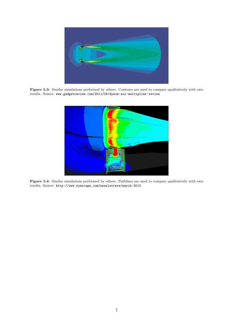
Figure 5.3: Similar simulations performed by others. Contours are used to compare qualitatively with ownresults. Source: www.gadgetreview.com/2011/08/dyson-air-multiplier-review

Figure 5.4: Similar simulations performed by others. Pathlines are used to compare qualitatively with ownresults. Source: http://www.symscape.com/newsletters/march-2012

7