flow assurance & operability - · pdf filemek 4450 - fmc technologies flow assurance &...
TRANSCRIPT

MEK 4450 - FMC TECHNOLOGIES
Flow Assurance & Operability A System Perspective
Revision 5
Tine Bauck Irmann-Jacobsen, Bjarte Hægland and Arnaud Sanchis
10/19/2015
The objective of compendium is to give an introduction to system design, from a flow assurance point of view, for the development of subsea oil and gas fields. The main phases of the design process are presented. Main Flow Assurance related subjects of interest are presented in brief.

1
1 Table of Contents 2 Introduction .......................................................................................................................................... 4
3 Subsea Fields ......................................................................................................................................... 4
3.1 Types of fields ........................................................................................................... 6
3.2 Engineering phases ................................................................................................... 7
3.2.1 Feasibility/concept phase ......................................................................................... 7
3.2.2 Front End Engineering Design (FEED) phase ............................................................ 7
3.2.3 Engineering Procurement Construction (EPC) phase ............................................... 8
3.2.4 Operation.................................................................................................................. 8
3.2.5 Tail end production / Increased Oil (gas) recovery (IOR) ......................................... 8
4 Main Flow Assurance challenges in system design .............................................................................. 9
5 Fluid properties ................................................................................................................................... 13
6 Pipe flow ............................................................................................................................................. 15
6.1 Derivation of conservation of momentum for single phase flow in pipe .............. 15
6.2 Darcy – Weisbach friction factors and Moody chart .............................................. 19
6.3 Pressure drop ......................................................................................................... 21
6.4 Water hammer ....................................................................................................... 24
6.4.1 Joukowsky equation ............................................................................................... 24
6.4.2 Unsteady flow in pipes ........................................................................................... 27
7 Heat transfer ....................................................................................................................................... 31
7.1 Conductive heat transfer ........................................................................................ 31
7.2 Convection heat transfer ........................................................................................ 31
7.3 Radiation heat transfer ........................................................................................... 31
7.4 Thermal resistance ................................................................................................. 32
7.4.1 1-dimensional plane conductive heat transfer ...................................................... 32
7.4.2 1-dimensional radial conductive heat transfer ...................................................... 33
7.4.3 Overall heat transfer coefficient ............................................................................ 35
7.5 Heat transfer in pipe flow ....................................................................................... 37
7.5.1 Heat loss for steady state pipe liquid flow ............................................................. 37
7.5.2 Heat loss for steady state pipe gas flow ................................................................. 38
7.5.3 Heat loss for steady state pipe multiphase flow .................................................... 38
7.5.4 Cool down of fluid filled pipe after shut-down (to be finished) ............................. 38

2
8 Multiphase flow .................................................................................................................................. 40
8.1 Flow regimes........................................................................................................... 40
8.2 Slugging................................................................................................................... 43
9 Hydrates .............................................................................................................................................. 45
9.1 Hydrate control strategy ........................................................................................ 47
9.1.1 Hydrate prevention ................................................................................................ 47
9.1.2 Hydrate control remediation .................................................................................. 52
10 Flow Induced vibrations ......................................................................................... 55
10.1 General definition ................................................................................................... 55
10.2 Fatigue .................................................................................................................... 55
10.3 Sources of Flow-Induced Vibrations ....................................................................... 56
10.3.1 Singing riser ............................................................................................................ 57
10.3.2 Acoustic pulsation in dead legs .............................................................................. 58
10.3.3 Multiphase flow in bended piping .......................................................................... 59
10.4 Analysis of Flow-Induced Vibrations ...................................................................... 60
11 Wax ......................................................................................................................... 61
12 Erosion .................................................................................................................... 64
12.1 Causes of erosion.................................................................................................... 64
12.1.1 Droplet erosion ....................................................................................................... 64
12.1.2 Cavitation ................................................................................................................ 65
12.1.3 Erosion corrosion .................................................................................................... 65
12.1.4 Sand production and erosion due to produced sand ............................................. 65
13 Overview simulation models in flow assurance ..................................................... 70
14 Field developments - Concept Selection ................................................................ 73
14.1 Types of fields ......................................................................................................... 73
14.2 Floater/Subsea........................................................................................................ 74
15 Examples of field developments with subsea process stations ............................. 77
15.1 Troll Pilot - liquid/liquid separation ........................................................................ 77
15.2 Tordis ...................................................................................................................... 79
15.3 Pazflor - Gas/Liquid Separation and Liquid Boosting ............................................. 81
15.4 Marlim .................................................................................................................... 83
16 Vocabulary .............................................................................................................. 85

3
17 Literature ................................................................................................................ 88
18 Attachments ........................................................................................................... 89
18.1 Water content in natural gas .................................................................................. 89

4
2 Introduction Flow assurance is a relatively new term in oil and gas industry. It refers to ensuring successful and
economical flow of hydrocarbon stream from reservoir to the point of sale. The primary goal of flow
assurance is to ensure production of hydrocarbons in a safe and reliable way and ensure operability
through the entire life of field.
Flow Assurance developed because of subsea development including shorter and longer flowlines
transporting of unprocessed multiphase flow.
The term Flow Assurance was first used by Petrobras in the early 1990s in Portuguese as Garantia do
Escoamento (pt::Garantia do Escoamento), meaning literally “Guarantee of Flow”, or Flow Assurance.
In order to guaranty feasible, safe and cost effective production for subsea oil and gas field Flow
Assurance needs to covers a number of special engineering fields and is an extremely diverse subject
matter.
In the system design for a subsea oil and gas development Flow Assurance take critical part in all phases
of the project. Flow assurance challenges increase with sea depth, tie-back distances, harsh
environment as well as more complex reservoir fluids.
The various phases of a subsea oil and gas development are presented herein. Some of the major Flow
Assurance focus points are presented and dwelled briefly into.
3 Subsea Fields Subsea fields are characterized by a large network of wells, flowlines and manifolds.
Subsea oil and gas field developments are usually split into Shallow water and Deepwater categories to
distinguish between the different facilities and approaches that are needed.
The term shallow water or shelf is used for shallow water depths where bottom-founded facilities like
jackup drilling rigs and fixed offshore structures can be used, and where saturation diving is feasible.
Deepwater is a term often used to refer to offshore projects located in water depths greater than
around 600 feet (200 m sea water depth), where floating drilling vessels and floating oil platforms are
used, and unmanned underwater vehicles are required as manned diving is not practical.
Shell completed its first subsea well in the Gulf of Mexico in 1961.
Subsea production systems can range in complexity from a single satellite well with a flowline linked to a
fixed platform, Floating Production Storage and Offloading (FPSO) unit or an onshore installation, to
complex subsea process stations and several wells on a template or clustered around a manifold, and
transferring to a fixed or floating facility, or directly to an onshore installation.

5
The development of subsea oil and gas fields requires specialized equipment. The equipment must be
reliable enough to safe guard the environment, and make the exploitation of the subsea hydrocarbons
economically feasible. The deployment of such equipment requires specialized and expensive vessels,
which need to be equipped with diving equipment for relatively shallow equipment work (i.e. a few
hundred meter water depth maximum), and robotic equipment for deeper water depths. Any
requirement to repair or intervene with installed subsea equipment is thus normally very expensive.
Subsea technology in offshore oil and gas production is a highly specialized field of application with
particular demands on engineering, simulation and flow assurance knowledge. Most of the new oil and
gas fields are located in deepwater and are generally referred to as deepwater systems. Development of
these fields sets strict requirements for verification of the various systems’ functions and their
compliance with current requirements and specifications, which is why flow assurance has a high focus
in these types of development.
Figure 1: Example subsea field system characterized by a large network of wells, flowlines and
manifolds.
Main drivers for field development of subsea systems
The main motivation for the development of an oil/gas field is in general to maximized
production of oil or gas from reservoir to receiving facilities.
The main parameters from a flow assurance perspective are the reservoir fluid properties,
pressure and temperature.
6
Main parameters for selection of system solution are technical feasibility, safety, reliability and
cost.
Main focus areas dealt with are hydrates, wax, erosion, flow induced vibrations and water
hammer.
The flow assurance specialist must be able to design multiphase systems to ensure the safe,
uninterrupted transport of reservoir fluids to the processing facilities.
Keywords for subsea design are robustness, simplicity and efficiency. The equipment needs to
operate for decades with a minimum of down time or required maintenance.
3.1 Types of fields Fields are divided between types of production fluid e.g. oil or gas fields. In both cases the fluid will be
multiphase incorporating; oil, gas and water, but in a typical gas field the amount of gas compare to
liquid or oil will be dominant.
The production fluid is characterized by the gas oil ration (GOR) and gas liquid ratio (GLR). The GOR is
calculated based on standard conditions of the fluid rates while the GLR are usually based on
calculations of the actual fluid rates.
The fields are also divided in Old (Brown) and New (Green) fields. New developments of old fields are
often called increased oil (gas) recovery developments, as the objective is to recover more of the fluid
from the reservoir.
All fields are unique which means that the combination of fluid properties, pressures and temperatures
and field layout must be evaluated for each new field.
Some new fields are difficult accessible fields
very deep water
extremely deep reservoirs
extremely shallow reservoirs
long tie-ins
heavy oil with high viscosity
high temperature/high pressure reservoirs
low temperature reservoirs

7
3.2 Engineering phases A field is developed in several phases. Flow Assurance is an important part of each phase from concept
evaluation to tail end production.
Figure 2: Phases in a field development
3.2.1 Feasibility/concept phase
In the feasibility and concept phase screening of different alternative solutions are one of the main
activities. Possible showstoppers and opportunities for each option considered shall be identified. Flow
Assurance contributes with system understanding, identification of specific challenges into this unique
system related to fluid properties, multiphase handling and driving pressure. An outline of the
production and process system for each option is created.
Among the various development options screened the ones deemed feasible are then ranked among
many things with respect to safety, cost, technologic maturity and operability. One or two options are
then moved into the FEED phase.
Main type of tools used aiding flow assurance:
1D multiphase simulations software like; FlowManager™ or OLGA. Mainly looking at
pressure and temperature drops and flow regimes in flow lines. Heavy slugging should be
avoided.
3.2.2 Front End Engineering Design (FEED) phase
In the FEED phase a concept is usually selected (or it might be a ranking of concepts) and the challenges
identified in the concept phase are investigated in more detail. Further Flow Assurance challenges are
identified and mitigating actions are identified. The Flow Assurance engineer needs to supply strategies
to handle a multitude of issues such as erosive wear, flow induced vibrations, hydrates, wax, thermal
cold spots and dead legs, pressure drop and temperature drop among many things. It shall be concluded
on whether an issue can be solved in the detailed engineering phase or not.
Main type of tools used aiding flow assurance:
Concept Evaluations
FEED Detailed Engineering
Operation
Tail end production

8
1D multiphase simulations softwares; FlowManager™ or OLGA
Sand erosion screening tools; DNV-RP-O501 or Tulsa
Flow induced vibration screening; Energy Institute guideline and/or detailed structural
analysis
Thermal design tools
3.2.3 Engineering Procurement Construction (EPC) phase
In the EPC phase detailed analysis is carried out to ensure that all Flow Assurance requirements are
implemented to the specification of the customer. Also operational monitoring systems and
development of process procedures are part of the flow assurance responsibility.
Main type of tools used aiding flow assurance:
1D multiphase simulations softwares; FlowManager™ or OLGA
Sand erosion screening tools; DNV-RP-O501 or Tulsa and CFD sand erosion simulations
Flow induced vibration screening; Detailed structural analysis
Thermal design tools: thermal finite element analysis (FEA) and thermal CFD simulations
3.2.4 Operation
During operation of the field the flow assurance engineer is involved in online monitoring of the system.
Provide advice on flow assurance, operating procedures, surveillance, production optimization and de-
bottlenecking for fields in operation.
3.2.5 Tail end production / Increased Oil (gas) recovery (IOR)
Tail end production can result in an increased oil (gas) recovery development which starts all over from
concept evaluations and through a FEED, detailed engineering and new operation. Evaluations from the
first engineering phase must then be taken into the design of the new engineering.

9
4 Main Flow Assurance challenges in system design
Figure 3: Field schematic showing flow assurance challenges that need to be addressed in a subsea
multiphase production system

10
Table 1: Includes an overview of the main flow assurance issues and the tasks and analysis to be
performed for any system
Potential issues Evaluations / studies to be performed
Hydrate formation Develop hydrate management strategy
(Understand actual Company hydrate strategy if already existing)
Requirement of insulation
Freezing valves (valve design)
Drainage of equipment
Deadleg design
Ensure MEG/Methanol distribution (if actual)
MEG/methanol injection points
Wax deposits Establish WAT (Wax Appereance Temperature)
Insulation requirements
Pigging requirements
Multiphase flow
Branching
Branching
Ensure MEG distribution
Ensure liquid distribution
Flow regime
Fluid properties Establish or verify hydrate formation temperature
Establish or verify wax appearance temperature
Validate PVT data stated from company and ensure consistency to
viscosities and densities
Establish composition to be used in the different simulations tools;
HYSYS steady state, OLGA, CFD, HYSYS dynamics,
Calculations input to hydrate formation potential and gas ingress

11
Potential issues Evaluations / studies to be performed
Sand production
Erosion (see erosion)
Sand accumulation
Erosion due to sand
production
General assessment with DNV-RP-0501
Detailed investigation with CFD
Sand management
Steering criteria for production
Thermal requirement General assessment based on hydrate strategy, wax management and
assessment of influence of temperature on process as separation /
compression
Insulation
No-touch time
Cool down time
Detailed investigation of thermal requirements with FEA and CFD
Multiphase simulations Conceptual screening
Bottlenecking of pressure drop
Flow regime
investigation
Control of flow regime in flowlines
Control of flow regime inlet separation equipement investigated by
simulations/testing
OLGA/FlowManager™ dynamic simulations to investigate inlet
conditions
Terrain slugging in
flowline
OLGA and Flow Manager simulations in upstream and downstream
flowlines
Simulation model, OLGA /Flow Manager, corresponding to actual
geometries inlet, on station and outlet

12
Potential issues Evaluations / studies to be performed
Riser slugging and
stability
Simulations by OLGA and Flow Manager to investigate oscillation
velocities related to sand transport and process control
Simulations of after flushing outlet conditions
Gas lift
Dynamic simulations Impact from shut-down, start-up, sensitivity to flow regimes are
incorporated in the simulations and in the flow assurance strategies
Operational Philosophy Hydrate strategy, de-pressurization and other Flow Assurance issues
are properly handled in operational procedures with special emphasize
on shut-down and start-up
Water Hammer effects Analysis to be performed
Chemical injection
points and PDT
instrumentation
General requirements
Emulsion Company premises: Downhole injection of de-emulsifiers through gas-
lift valve
The use of de-emulsifiers affects the design of the separation
equipment
Corrosion Material selection
Asphaltenes Evaluation composition and chemicals
Flow induced vibrations Evaluations flow induced vibrations
Monitoring Online FAS (Flow Assurance System)
CPM (Conditioning Performance Monitoring)

13
Figure 4: Potential field challenges
5 Fluid properties When an oil and/or gas field is discovered several exploration and appraisal wells are drilled to
characterize the reservoir. Several samples of the reservoir fluid are taken. These are tested in labs and
characterized and form the basis for determining the fluid properties for the field.
Fluid compositions are entered into a PVT equation of state software such as PVTsim or MultiFlash and
tuned against fluid properties at reservoir conditions. Once the fluid has been properly characterized
and tuned PVT simulations may determine the fluid properties for all operational conditions and is the
main input tool providing input data to:
Reservoir simulation tools
Pipeline multiphase simulations tools
Process simulation tools
Physical fluid properties needed for detailed FEA and CFD simulations.
Hydrate management by providing hydrate equilibrium curves and identifying required amount of
hydrate inhibitor.
14
Wax and asphaltenes management by providing wax appearance temperatures
Preliminary temperature drop calculations over production chokes.
15
6 Pipe flow
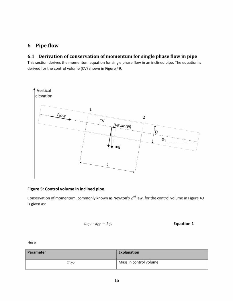
6.1 Derivation of conservation of momentum for single phase flow in pipe This section derives the momentum equation for single phase flow in an inclined pipe. The equation is
derived for the control volume (CV) shown in Figure 49.
CV
1
2Flow
mg sin(Θ)
mg
Θ
L
D
Vertical elevation
Figure 5: Control volume in inclined pipe.
Conservation of momentum, commonly known as Newton’s 2nd law, for the control volume in Figure 49
is given as:
𝑚𝐶𝑉 ∙ 𝑎𝐶𝑉 = 𝐹𝐶𝑉 Equation 1
Here
Parameter Explanation
𝑚𝐶𝑉 Mass in control volume
16
Parameter Explanation
𝑎𝐶𝑉 Acceleration of the fluid particle defined by the
control volume.
𝐹𝐶𝑉 Sum of all forces acting on the control volume.
The rate of momentum change on the left hand side of Equation 2 for the control volume may be
defined as
𝑚𝐶𝑉. 𝑎𝐶𝑉 = 𝜌𝐿𝐴𝑑𝑢
𝑑𝑡= 𝜌𝐿
𝑑𝑄
𝑑𝑡 Equation 2
Here
Parameter Explanation
𝜌 Average (constant) density of fluid in control
volume.
𝐿 Length of control volume.
𝐴 Average (constant) cross-sectional area of the
control volume
𝑢 Average velocity in control volume.
𝑄 Average volume flow rate in control volume.
The forces acting on the control volume are:
- Normal acting pressure forces
- Shear stress frictional force
- Gravitational force
Hence the total force on the right hand side of Equation 2 for the control volume is

17
𝐹𝐶𝑉 = 𝑃1𝐴 − 𝑃2𝐴 +𝑚𝑔 sin(𝜃) − 𝜏𝑤𝜋𝐿𝐷 Equation 3
Here
Parameter Explanation
𝐴 =1
4𝜋𝐷2
Cross-sectional area (assumed constant) in control
volume.
𝑃1 Pressure at location 1
𝑃2 Pressure at location 2
𝑚 = 𝜌𝐿𝐴 Mass in control volume
𝜌 Average (constant) density of fluid in control
volume.
𝐿 Length of control volume.
𝐴 Average (constant) cross-sectional area of the
control volume
𝑔 Gravitational acceleration.
𝐷 Diameter of control volume (assumed constant)
𝜃 Angle of inclination for the pipe
sin(𝜃) =∆ℎ
𝐿
Sin-function of angle of inclination.
∆ℎ Elevation change along pipe section defined by the
control volume.
𝜏𝑤 Wall shear stress
The wall shear stress may be expressed introducing Darcy – Weisbach friction factor 𝑓:

18
𝜏𝑤 =1
8𝑓𝜌𝑢2 Equation 4
The frictional force term may be expressed as:
𝐹𝜏 = 𝜏𝑤𝜋𝐿𝐷 =1
8𝑓𝜌𝑢2𝜋𝐿𝐷 =
1
4𝜋𝐷2 ∙
𝑓𝐿
𝐷∙1
2𝜌𝑢2 = 𝐴 ∙
𝑓𝐿
𝐷∙1
2𝜌𝑢2 Equation 5
Here 𝑃𝜏 =𝑓𝐿
𝐷∙1
2𝜌𝑢2 is the commonly used term for pressure drop due to friction in a pipe.
The sum of forces acting on the control volume may be summarized as:
𝐹𝐶𝑉 = 𝐴 ∙ (𝑃1 − 𝑃2 + 𝜌𝑔∆ℎ −𝑓𝐿
𝐷∙1
2𝜌𝑢2) Equation 6
Combining Equation 2 and Equation 6 yields the momentum equation
𝑑𝑄
𝑑𝑡=
𝐴
𝜌𝐿∙ (𝑃1 − 𝑃2 + 𝜌𝑔∆ℎ −
𝑓𝐿
𝐷∙1
2𝜌𝑢2) Equation 7
For incompressible and steady state the above equation reduces to
∆𝑃 = 𝑃1 − 𝑃2 = −𝜌𝑔∆ℎ +𝑓𝐿
𝐷∙1
2𝜌𝑢2 Equation 8
The pressure drop is expressed as by two terms: a gravitational contribution and a frictional
contribution.

19
6.2 Darcy – Weisbach friction factors and Moody chart The Darcy – Weisbach friction factor (Equation 9) may be expressed as follows:
Laminar flow 𝑅𝑒 < 2300 𝑓 =64
𝑅𝑒
Equation 9 Turbulent flow
(Haaland) 𝑅𝑒 ≥ 2300 𝑓 = [−1.8 log10 ((
휀
𝐷 ∙ 3.7)1.11
+6.9
𝑅𝑒)]
−2
Here
Parameter Explanation
𝑓 Darcy – Weisbach friction factor
휀 Wall roughness
𝐷 Internal pipe diameter
𝑅𝑒 =𝜌𝑢𝐷
𝜇
Dimensional less Reynolds number
𝜌 Fluid density
𝑢 Fluid velocity
Equation 9 utilizes commonly known correlations for friction factors for the laminar and turbulent flow
regimes, however the transition between laminar flow regime and turbulent flow regime is set at a
Reynolds number of 2300. Equation 9 does not properly address the transitional flow regimes observed
moving from laminar to turbulent flow. The implementation of the friction factors in Equation 9 is not
recommended as it is known to cause numerical instabilities due to the discontinuity in the friction
factor moving from laminar flow regime into the turbulent flow regime. In reality no such discontinuity
occurs; a smooth transition between laminar and turbulent flow regime is seen; see reference [5].

20
Figure 6; Moody diagram for Equation 9; discontinuous friction factor.
Transitional flow regime occurs for Reynolds numbers in the range 2000 < 𝑅𝑒 < 4000; see reference
/4/ and /5/. It is recommended to calculate the friction factor for the laminar, transitional and turbulent
flow regimes as detailed in reference [5] chapter 6.3 to eliminate discontinuities in the Darcy – Weisbach
friction factor. Figure 51 is illustrating a smooth transition in friction factors from the laminar and
turbulent flow regimes.

21
Figure 7: Moody diagram with transitional flow regime accounted for.
6.3 Pressure drop In the start the natural gas or oil in a reservoir flows to the surface by the reservoir pressure. When the
pressure drop between reservoir and receiving facilities gets too large to overcome the pressure drop in
the system, the wells stop producing and the flow in the line will stop. The life of the well is a dynamic
process and often water production from the wells increase in late life. The wells will be closed down
when the cost of handling the water production is higher than the value of the oil and gas produced.
During the production the reservoir will be more and more drained and the reservoir pressure will
decrease. The pressure gradient from well head to receiving facilities governs the production rate. It is
therefore important to reduce the pressure drop between the well head and the receiving facilities.
The pressure drop is influenced by many different parameters in multiphase flow. All of these
parameters need to be evaluated and calculated in all parts of a system. The following parameters have
impact on the pressure drop in multiphase production systems.
Frictional pressure drop

22
o For long flowlines the contribution from the friction between flow and fluid is the most
dominant parameter that causes pressure drop (see exercises).
Hydraulic resistance in pipe components
o There are contributions to pressure drop from every bend, valve and process module in
a system. Especially on a subsea station these impacts need to be calculated and
reduced to a minimum. In some cases a high consciousness of this can result in an
optimal design with regards to minimum pressure drop.
Gravity forces
o The weight of the height column of multiphase will be important in the vertical part of
the well, long flowlines and risers (see exercises)
Fluid, amount of liquid
o In multiphase flow the fluid phases will vary in different parts of the system and in
different parts of production life according to temperature, pressure and rates. As can
be seen from Equation 2, density is one of the parameters that influence on pressure
drop, and in general more liquid give a higher pressure drop than very dry gas. This
means i.e. that when a well start to produce more water along with oil and/or gas, the
pressure drop will increase resulting in lower production rates and hence even lower
gas/and or oil rates.
Length of flowline
o In some fields the distance to shore from field is a governing parameter. Solutions as
separation of liquid and gas and boosting with pump and compressor are evaluations to
be done to see what is necessary to get a driving pressure in the system.
Velocity
o Higher velocities increase pressure drop. This is important to evaluate in line sizing.
Temperature increase actual flow
o Water is nearly incompressible and the impact from temperature on the actual flow is
low. This is not the case in gas, which is highly compressible. The actual flow will
increase with higher temperature and resulting in a higher velocity, which again impacts
on the pressure drop.
Density
o The density in multiphase will be a function of the rates of the three phases, the
temperature and pressure.

23
Contribution from gravity forces on pressure drop
Pres − Pwell = 𝑔∫ 𝜌(𝑦)d𝑦ℎ
0
Equation 10
Contribution from friction on pressure drop (Darcy-Weisbach)
∆P = 𝑓𝐿
𝐷
𝜌 ∙ 𝑈𝑏2
2 Equation 11
Figure 8: Steady state pressure drop and hold-up versus production rate

24
6.4 Water hammer The presentation of water hammer theory in this section follows closely the presentation in Hydraulics
of pipeline systems [8].
When velocities in a pipe system changes so rapidly that the elastic properties of the pipe and liquid
must be considered in an analysis, we have a hydraulic transient commonly known has water hammer.
Water hammer commonly occurs when a valve is closed quickly at an end of a pipeline system, and a
pressure wave propagates in the pipe. It may also be known as hydraulic shock.
6.4.1 Joukowsky equation
Consider the simple pipe flow below with constant liquid flow towards the right with velocity V. The
valve positioned downstream is initially open.
Figure 9: Constant liquid flow in a straight pipe.
Consider further the event that the downstream valve suddenly closes. The flowing liquid immediately
upstream the valve will come to an abrupt stop and the pressure upstream the valve will have to
increase an amount just sufficient to reduce the momentum of the moving liquid to zero. The abrupt
valve closure causes an increase in pressure which will travel in the upstream direction. The question is
how large is the pressure increase due to the abrupt valve closure?
As the valve closes the pressure upstream the valve increases to overcome the momentum of the liquid.
As the pressure increases the liquid gets compressed and the liquid density increases. Also the pressure
increase slightly enlarges the pipe.
Assume the pressure wave travels upstream with a velocity 𝑎. Consider Figure 20 showing an unsteady
control volume centered on the pressure wave traveling upstream the pipe after the valve closure.
V
L
Constant upstream pressure Valve

25
Figure 10: Unsteady control volume for water hammer analysis
The flow is not steady as the control volume is moving, so the linear equations for steady flow do not
apply. Instead it is possible to assume the reference system moves towards the left with a velocity 𝑎 as
depicted in Figure 21:
Figure 11: Steady flow control volume for water hammer analysis.
Let's detail the forces acting on the control volume in further details
V
δL
V+ΔV a
V+a
δL
V+ΔV+a

26
Figure 12: Steady flow control volume for water hammer with all forces shown.
The wall shear force 𝐹𝑠 due to friction will be ignored. Also we only consider relatively strong pipe
materials such as steel the pipe bulge is very small and so 𝐹3 is neglected. We assume uniform flow
velocity and consider the linear momentum equation parallel to the pipe for the control volume in
Figure 22:
∑𝐅 = Qρ(𝑉out − 𝑉in) Equation 12
𝐹1 − 𝐹2 = 𝑄𝜌[(𝑉 + ∆𝑉 + 𝑎) − (𝑉 + 𝑎)] = 𝑄𝜌∆𝑉
Equation 13
Here 𝑄 = (𝑉 + 𝑎)𝐴. Assume the pressure at (1) is 𝑝0 then the pressure at (2) is 𝑝0 + ∆𝑝. Then Equation
5 reads:
𝑝0𝐴 − (𝑝0 + ∆𝑝)(𝐴 + 𝛿𝐴) = (𝑉 + 𝑎)𝐴𝜌∆𝑉
Equation 14
The increase in pipe cross sectional area 𝛿𝐴 is very small and can be ignored so the pressure increase
can be simplified as
∆𝑝 = −(𝑉 + 𝑎)𝜌∆𝑉 = −𝜌𝑎∆𝑉 (1 +𝑉
𝑎) Equation 15
V+a
δL
V+ΔV+a
F3
Fn
Fs
F1
F2
(1) (2)
Area: A
Density: ρ
Area: A+δA
Density: ρ+δρ
27
In most rigid pipes the value of 𝑉/𝑎 is very small and the pressure increase due to a decrease in velocity
∆𝑉 is
∆𝑝 ≈ −𝜌𝑎∆𝑉
Equation 16
The pressure pulse wave speed 𝑎 is denoted the sonic speed or speed of sound in the fluid filled pipe.
The sonic speed is dependent on the fluid bulk modulus, elasticity of the pipe and the amount of
entrapped gas present in the liquid system.
Equation 16 is sometimes referred to as Joukowsky's equation and gives the maximum amplitude of the
pressure pulse due to an abrupt valve closure.
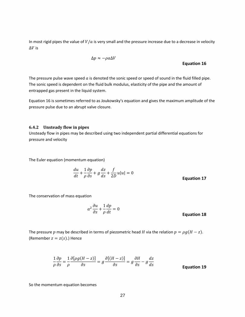
6.4.2 Unsteady flow in pipes
Unsteady flow in pipes may be described using two independent partial differential equations for
pressure and velocity
The Euler equation (momentum equation)
𝑑𝑢
𝑑𝑡+1
𝜌
𝜕𝑝
𝜕𝑠+ 𝑔
𝑑𝑧
𝑑𝑠+
𝑓
2𝐷𝑢|𝑢| = 0
Equation 17
The conservation of mass equation
𝑎2𝜕𝑢
𝜕𝑠+1
𝜌
𝑑𝑝
𝑑𝑡= 0
Equation 18
The pressure 𝑝 may be described in terms of piezometric head 𝐻 via the relation 𝑝 = 𝜌𝑔(𝐻 − 𝑧).
(Remember 𝑧 = 𝑧(𝑠).) Hence
1
𝜌
𝜕𝑝
𝜕𝑠=1
𝜌
𝜕[𝜌𝑔(𝐻 − 𝑧)]
𝜕𝑠= 𝑔
𝜕[(𝐻 − 𝑧)]
𝜕𝑠= 𝑔
𝜕𝐻
𝜕𝑠− 𝑔
𝑑𝑧
𝑑𝑠
Equation 19
So the momentum equation becomes

28
𝑑𝑢
𝑑𝑡+ 𝑔
𝜕𝐻
𝜕𝑠+
𝑓
2𝐷𝑢|𝑢| = 0
Equation 20
The equation for conservation of mass becomes
𝑎2𝜕𝑢
𝜕𝑠+ 𝑔
𝑑𝐻
𝑑𝑡= 0
Equation 21
The total time derivatives in Equation 20 and Equation 21 are defined as
𝑑
𝑑𝑡=
𝜕
𝜕𝑡+ 𝑢
𝜕
𝜕𝑠
Equation 22
So both equations involve non-linear terms. For the moment let us assume the linear terms in the
momentum and the conservation of mass equation are larger than the non-linear terms in addition to
the non-linear friction term. We may evaluate later the consequences of this simplification. The
simplified equations become
𝜕𝑢
𝜕𝑡+ 𝑔
𝜕𝐻
𝜕𝑠= 0
Equation 23
and
𝑎2𝜕𝑢
𝜕𝑠+ 𝑔
𝜕𝐻
𝜕𝑡= 0
Equation 24
The equations are linear so cross-differentiation will low us to eliminate one of the unknowns
𝑔𝜕2𝐻
𝜕𝑡2= −𝑎2
𝜕2𝑢
𝜕𝑡𝜕𝑠= −𝑎2
𝜕2𝑢
𝜕𝑠𝜕𝑡= −𝑎2 (−𝑔
𝜕2𝐻
𝜕𝑠2) = 𝑔𝑎2
𝜕2𝐻
𝜕𝑠2 Equation 25
Hence the piezometric head is governed by the wave equation
𝜕2𝐻
𝜕𝑡2= 𝑎2
𝜕2𝐻
𝜕𝑠2 Equation 26

29
It can be shown that the velocity 𝑢 also is governed by this equation.
In Equation 26 the parameter 𝑎 is known as the wave propagation speed. Assuming 𝐻 = 𝐻(𝑠, 𝑡) and
introducing as new independent variables 𝑣 = 𝑡 + 𝑠/𝑎 and 𝑤 = 𝑡 − 𝑠/𝑎 we get
𝜕𝐻
𝜕𝑡=𝜕𝐻
𝜕𝑣
𝜕𝑣
𝜕𝑡+𝜕𝐻
𝜕𝑤
𝜕𝑤
𝜕𝑡=𝜕𝐻
𝜕𝑣+𝜕𝐻
𝜕𝑤 Equation 27
And
𝜕2𝐻
𝜕𝑡2=
𝜕
𝜕𝑡(𝜕𝐻
𝜕𝑣+𝜕𝐻
𝜕𝑤) =
𝜕2𝐻
𝜕𝑣2𝜕𝑣
𝜕𝑡+
𝜕2𝐻
𝜕𝑤𝜕𝑣
𝜕𝑤
𝜕𝑡+
𝜕2𝐻
𝜕𝑣𝜕𝑤
𝜕𝑣
𝜕𝑡+𝜕2𝐻
𝜕𝑤2
𝜕𝑤
𝜕𝑡
𝜕2𝐻
𝜕𝑡2=𝜕2𝐻
𝜕𝑣2+ 2
𝜕2𝐻
𝜕𝑣𝜕𝑤+𝜕2𝐻
𝜕𝑤2
Equation 28
In a similar fashion
𝜕𝐻
𝜕𝑠=𝜕𝐻
𝜕𝑣
𝜕𝑣
𝜕𝑠+𝜕𝐻
𝜕𝑤
𝜕𝑤
𝜕𝑠=1
𝑎
𝜕𝐻
𝜕𝑣−1
𝑎
𝜕𝐻
𝜕𝑤 Equation 29
And
𝜕2𝐻
𝜕𝑠2=
𝜕
𝜕𝑠(1
𝑎
𝜕𝐻
𝜕𝑣−1
𝑎
𝜕𝐻
𝜕𝑤) =
1
𝑎(𝜕2𝐻
𝜕𝑣2𝜕𝑣
𝜕𝑠+
𝜕2𝐻
𝜕𝑤𝜕𝑣
𝜕𝑤
𝜕𝑠) −
1
𝑎(𝜕2𝐻
𝜕𝑣𝜕𝑤
𝜕𝑣
𝜕𝑠+𝜕2𝐻
𝜕𝑤2
𝜕𝑤
𝜕𝑠)
𝜕2𝐻
𝜕𝑠2=1
𝑎(1
𝑎
𝜕2𝐻
𝜕𝑣2−1
𝑎
𝜕2𝐻
𝜕𝑤𝜕𝑣) −
1
𝑎(1
𝑎
𝜕2𝐻
𝜕𝑣𝜕𝑤−1
𝑎
𝜕2𝐻
𝜕𝑤2) =
1
𝑎2(𝜕2𝐻
𝜕𝑣2− 2
𝜕2𝐻
𝜕𝑤𝜕𝑣+𝜕2𝐻
𝜕𝑤2)
Equation 30
So by introducing 𝑣 and 𝑤 as new independent variables Equation 26 reduces to
4𝜕2𝐻
𝜕𝑣𝜕𝑤= 0 Equation 31
The general solution to Equation 31 is a solution
𝐻 = 𝐻0 + 𝐹1(𝑣) + 𝐹2(𝑤) = 𝐻0 + 𝐹1 (𝑡 +𝑠
𝑎) + 𝐹2 (𝑡 −
𝑠
𝑎) Equation 32
Here 𝐻0 is a constant and 𝐹1 is a function of 𝑣 and 𝐹2 is a function of 𝑤.
Consider 𝐹1, if the time passes from 𝑡1 to 𝑡2 = 𝑡1 + 𝛿𝑡 the function 𝐹1 has the same value if
𝑡1 +𝑠1𝑎= 𝑡2 +
𝑠2𝑎
Equation 33
Or if

30
𝑠2−𝑠1𝑎
= −(𝑡2 − 𝑡1) = −𝛿𝑡 Equation 34
So as time advances the argument 𝑡 +𝑠
𝑎 remains constant if
𝑠
𝑎 decreases with the same amount as the
time increases. So 𝐹1 is a leftward moving wave with an absolute velocity 𝑎. In the same fashion it can
be argued that 𝐹2 is a rightward moving wave with absolute velocity 𝑎. The general solution to Equation
18 is a superposition of left and right moving waves, moving at absolute velocity 𝑎.
In deriving Equation 26 nonlinear terms in the conservation of momentum equation and the mass
conservation equation were ignored. These terms are
𝑢𝜕𝑢
𝜕𝑠, and 𝑢
𝜕𝐻
𝜕𝑠
Equation 35
Let us assume a scaling 𝑠~𝑎 ∙ 𝑡 to the terms in Equation 35 and we find
𝑢𝜕𝑢
𝜕𝑠~𝑢
𝑎
𝜕𝑢
𝜕𝑡
𝑢𝜕𝐻
𝜕𝑠~𝑢
𝑎
𝜕𝐻
𝜕𝑡
Equation 36
For almost all cases 𝑢 𝑎⁄ ≪ 1 and the convective terms are negligible. Only in rare cases were the
flowing velocity 𝑢 is comparable to the sonic velocity 𝑎 is it important to include the non-linear
convective terms.
31
7 Heat transfer
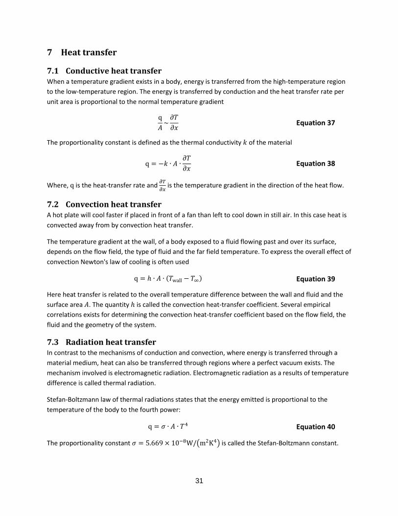
7.1 Conductive heat transfer When a temperature gradient exists in a body, energy is transferred from the high-temperature region
to the low-temperature region. The energy is transferred by conduction and the heat transfer rate per
unit area is proportional to the normal temperature gradient
q
𝐴~𝜕𝑇
𝜕𝑥 Equation 37
The proportionality constant is defined as the thermal conductivity 𝑘 of the material
q = −𝑘 ∙ 𝐴 ∙𝜕𝑇
𝜕𝑥 Equation 38
Where, q is the heat-transfer rate and 𝜕𝑇
𝜕𝑥 is the temperature gradient in the direction of the heat flow.
7.2 Convection heat transfer A hot plate will cool faster if placed in front of a fan than left to cool down in still air. In this case heat is
convected away from by convection heat transfer.
The temperature gradient at the wall, of a body exposed to a fluid flowing past and over its surface,
depends on the flow field, the type of fluid and the far field temperature. To express the overall effect of
convection Newton's law of cooling is often used
q = ℎ ∙ 𝐴 ∙ (𝑇wall − 𝑇∞) Equation 39
Here heat transfer is related to the overall temperature difference between the wall and fluid and the
surface area 𝐴. The quantity ℎ is called the convection heat-transfer coefficient. Several empirical
correlations exists for determining the convection heat-transfer coefficient based on the flow field, the
fluid and the geometry of the system.
7.3 Radiation heat transfer In contrast to the mechanisms of conduction and convection, where energy is transferred through a
material medium, heat can also be transferred through regions where a perfect vacuum exists. The
mechanism involved is electromagnetic radiation. Electromagnetic radiation as a results of temperature
difference is called thermal radiation.
Stefan-Boltzmann law of thermal radiations states that the energy emitted is proportional to the
temperature of the body to the fourth power:
q = 𝜎 ∙ 𝐴 ∙ 𝑇4 Equation 40
The proportionality constant 𝜎 = 5.669 × 10⁻⁸W/(m2K4) is called the Stefan-Boltzmann constant.

32
The Stefan-Boltzmann law applies to black bodies and only governs radiation emitted from the body.
The net radiant exchange between two surfaces is
q = 𝐹𝜖 ∙ 𝐹𝐺 ∙ 𝜎 ∙ 𝐴 ∙ 𝑇4 Equation 41
Here 𝐹𝜖 is emissivity and 𝐹𝐺 is a geometric view factor.
7.4 Thermal resistance
7.4.1 1-dimensional plane conductive heat transfer
For a plane wall the heat transfer across the wall can be expressed as
q = −𝑘 ∙ 𝐴
∆𝑥∙ (𝑇2 − 𝑇1) Equation 42
Figure 13 Heat transfer across plane wall
The heat transfer can be considered as a flow, and the combination of thermal conductivity,
thickness of material and area as resistance to this flow. The temperature difference is the
potential or driving force for heat flow:
heat flow =thermal potential difference
thermal resistance Equation 43
This relation is similar to Ohm's law in electric-circuit theory.
T1
T2
q q
1 2
q
T1 T
2
R
∆𝑥
𝑘 ∙ 𝐴

33
If more than one material is present as depicted in Figure 14 the heat flow may be written in
terms of the temperature difference over each of the layers
q = −𝑘𝐴 ∙ 𝐴
∆𝑥𝐴∙ (𝑇2 − 𝑇1) = −
𝑘𝐵 ∙ 𝐴
∆𝑥𝐵∙ (𝑇3 − 𝑇2) = −
𝑘𝐶 ∙ 𝐴
∆𝑥𝐶∙ (𝑇4 − 𝑇3) Equation 44
The heat flow across the multilayer wall can be expressed as
q =𝑇1 − 𝑇4
∆𝑥𝐴𝑘𝐴 ∙ 𝐴
+∆𝑥𝐵𝑘𝐵 ∙ 𝐴
+∆𝑥𝐶𝑘𝐶 ∙ 𝐴
=𝑇1 − 𝑇4
𝑅𝐴 + 𝑅𝐵 + 𝑅𝐶
Equation 45
In general the 1-dimensional heat flow can be written
q =∆𝑇
∑ 𝑅layerlayers Equation 46
Figure 14 Heat transfer across multiple layer plane wall
7.4.2 1-dimensional radial conductive heat transfer
Consider a long cylinder with inner radius and outer radius. For cylinders with length very large
compared to diameter it may be assumed that the heat flows only in radial direction. At a radius 𝑟 the
area the heat for the heat flow is 𝐴 = 2𝜋𝑟𝐿. Fouries's law for radial heat transport reads
T1
1 2
q
T1 T
2
RA
∆𝑥𝐴𝑘𝐴 ∙ 𝐴
T2
T3
T4
3 4
T3
RB
T4
RC
∆𝑥𝐵𝑘𝐵 ∙ 𝐴
∆𝑥𝐶𝑘𝐶 ∙ 𝐴

34
q = −kAdT
dr= −2𝜋𝑘𝑟𝐿
dT
dr Equation 47
By integration it is readily shown that
q =2𝜋𝑘𝐿
𝑙𝑛 (𝑟𝑜𝑟𝑖)(𝑇𝑖 − 𝑇𝑜) Equation 48
Figure 15 1-dimensional heat flow in radial direction
In a similar fashion the heat flow in radial direction through the multilayered pipe in Figure 16 is
q =2𝜋𝑘𝐴𝐿
𝑙𝑛 (𝑟2𝑟1)(𝑇1 − 𝑇2) =
2𝜋𝑘𝐵𝐿
𝑙𝑛 (𝑟3𝑟2)(𝑇2 − 𝑇3) =
2𝜋𝑘𝐶𝐿
𝑙𝑛 (𝑟4𝑟3)(𝑇3 − 𝑇4) Equation 49
r0 ri
r
L
q
Ti T
o
R
𝑙𝑛(𝑟𝑜
𝑟𝑖 )
2𝜋 ∙ 𝑘 ∙ 𝐿

35
or in terms of total resistance
q =(𝑇1 − 𝑇4)
𝑅𝐴 + 𝑅𝐵 + 𝑅𝐶=
2𝜋𝐿(𝑇1 − 𝑇4)
𝑙𝑛 (𝑟2𝑟1)
𝑘𝐴+𝑙𝑛 (
𝑟3𝑟2)
𝑘𝐵+𝑙𝑛 (
𝑟4𝑟3)
𝑘𝐶
Equation 50
Figure 16 1-dimensional heat flow in radial direction through multilayer pipe
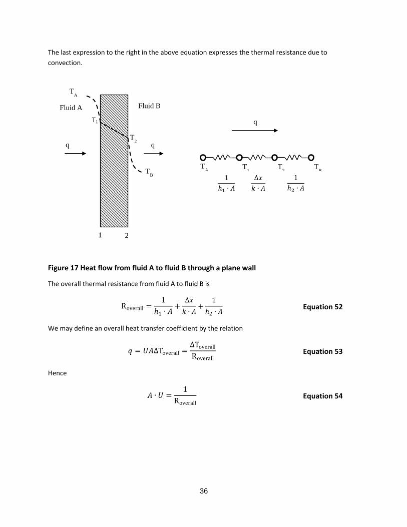
7.4.3 Overall heat transfer coefficient
Consider Figure 17 showing the heat flow from a fluid denoted A through a plane wall to a fluid denoted
B. We know that the convection heat flow at wall 1 can be expressed as
q = ℎ1 ∙ 𝐴 ∙ (𝑇1 − 𝑇𝐴) =1
ℎ1 ∙ 𝐴∙ (𝑇1 − 𝑇𝐴) Equation 51
r1
r2 r
3
r4
A
B
C
T1
T2
T3
T4
36
The last expression to the right in the above equation expresses the thermal resistance due to
convection.
Figure 17 Heat flow from fluid A to fluid B through a plane wall
The overall thermal resistance from fluid A to fluid B is
Roverall =1
ℎ1 ∙ 𝐴+
∆𝑥
𝑘 ∙ 𝐴+
1
ℎ2 ∙ 𝐴 Equation 52
We may define an overall heat transfer coefficient by the relation
𝑞 = 𝑈𝐴∆Toverall =∆ToverallRoverall
Equation 53
Hence
𝐴 ∙ 𝑈 =1
Roverall Equation 54
T1
T2
q q
1 2
q
TA
TB
TA T
1
1
ℎ1 ∙ 𝐴
T2 T
B
∆𝑥
𝑘 ∙ 𝐴
1
ℎ2 ∙ 𝐴
Fluid A Fluid B

37
7.5 Heat transfer in pipe flow
7.5.1 Heat loss for steady state pipe liquid flow
Figure 18: Steady state flow in pipe section with heat loss to ambient
Consider the pipe section depicted above. Fluid is flowing at steady state through the pipe. The fluid
temperature changes over the length of the pipe as heat is either lost or gained from the ambient. The
heat balance for the heat section may be described by
�� ∙ 𝑐𝑝 ∙ (𝑇(𝑥 + 𝑑𝑥) − 𝑇(𝑥)) = �� ∙ 𝐶𝑝 ∙ 𝑑𝑇 = −𝑑𝑄 = −𝜋 ∙ 𝐷𝑖 ∙ 𝑈 ∙ (𝑇(𝑥) − 𝑇ambient) ∙ 𝑑𝑥 Equation 55
The above equation results in the simple differential equation
1
(𝑇(𝑥) − 𝑇ambient)∙ 𝑑𝑇 = −
𝜋 ∙ 𝐷𝑖 ∙ 𝑈
�� ∙ 𝐶𝑝∙ 𝑑𝑥 Equation 56
The solution to the above differential equation is
𝑇(𝑥) = 𝑇ambient+(𝑇(0) − 𝑇ambient) ∙ 𝑒−𝜋∙𝐷∙𝑈��∙𝐶𝑝
∙𝑥 Equation 57
Here
Parameter Explanation
𝑇(𝑥) Temperature along the pipeline [°C]
𝑇ambient Ambient temperature outside pipe [°C]
𝑈 Overall outer heat transfer coefficient defined at pipe ID [W/(m2K)]
𝐷 Inner pipe diameter (ID) [m]
dx
�� ��
𝑇(𝑥) 𝑇(𝑥 + 𝑑𝑥)
𝑑𝑄 = 𝜋 ∙ 𝐷 ∙ 𝑈 ∙ (𝑇 − 𝑇ambient) ∙ 𝑑𝑥
V D

38
Parameter Explanation
�� Mass flow rate of the fluid [kg/s]
𝐶𝑝 Heat capacity of the fluid [J/(kg K)]
7.5.2 Heat loss for steady state pipe gas flow
For gas flow the Joule Thompson effect of cooling due to pressure drop has to be accounted for. The
Joule Thomson cooling effect relates the adiabatic change in temperature for a gas resulting from
change in pressure, defined as JT=dT/dP [°C/bar]. Typically JT > 0, i.e. temperature drops with reduction
in pressure.
Note that for a gas pipeline the JT effect may cause gas temperatures below the ambient temperature.
𝑇(𝑥) = 𝑇ambient+(𝑇(0) − 𝑇ambient) ∙ 𝑒−𝜋∙𝐷∙𝑈��∙𝐶𝑝
∙𝑥− 𝐽𝑇 ∙ ∆𝑝 Equation 58
7.5.3 Heat loss for steady state pipe multiphase flow
For multiphase flow the above equation above can be used by introducing:
��mix = ��oil + ��gas + ��water Equation 59
𝐶𝑝mix=��oil ∙ 𝐶𝑝, oil + ��gas ∙ 𝐶𝑝, gas + ��water ∙ 𝐶𝑝, water
��mix
Equation 60
7.5.4 Cool down of fluid filled pipe after shut-down (to be finished)
In this section we develop a method for computing the cool down of fluid inside an insulated pipe. The
cool down of the fluid, pipe and insulation is related to the conservation of energy for each of the layers
(fluid, pipe and insulation).
Consider a general material. The temperature in the material is governed by:
𝑚 ∙ 𝐶𝑝 ∙𝑑𝑇material
𝑑𝑡= 𝑞IN − 𝑞OUT Equation 61
Here 𝑚 is the mass of the material, 𝐶𝑝+ the specific heat capacity of the layer, 𝑇material the average
temperature of the material, 𝑞IN is heat flow into the material and 𝑞OUT the heat flow from the material.

39
Consider the multilayered pipe in Figure 19. In what follows we will assume the temperature in mid-
layer of a material to be equal to the average temperature in the material. In order to determine the
heat flow in and out of each material layer we need to determine the radial heat flux in the multilayered
pipe. We start by defining the thermal resistances between the mid-points of two consecutive layers.
Figure 19: Multilayered pipe
r1
r2 r
3
r4
A
B
C
T1
T2
T3
T4

40
8 Multiphase flow Multiphase flow describes multi-component systems in which the interaction between the different
components has a major influence on the overall flow structure. In the oil and gas industry multiphase
flow is the combined flow of gas, condensate/oil and water in a pipe. There are very few cases in
multiphase flow in which the problem can be simplified and still retain the essential physics. Some
examples of how to simplify and derive at evaluations in multiphase problems are given in the exercises.
Numerical simulation models are therefore necessary tools for designing multiphase systems. There
exist several numerical simulation tools and models.
Figure 20: Multiphase flow; water, oil, gas
8.1 Flow regimes The behavior of the gas and liquid in a flowing pipe will exhibit various flow characteristics depending on
the gas pressure, gas velocity and liquid content, as well as orientation of the piping (horizontal, sloping
or vertical). The liquid may be in the form of tiny droplets or the pipe may be filled completely with
liquid. Despite the complexity of gas and liquid interaction, attempts have been made to categorize this
behavior. These gas and liquid interactions are commonly referred to as flow regimes or flow patterns.
Annular mist flow occurs at high gas velocities. A thin film of liquid is present around the annulus of the
pipe. Typically most of the liquid is entrained in the form of droplets in the gas core. As a result of
gravity, there is usually a thicker film of liquid on the bottom of the pipe as opposed to the top of the
pipe.
Stratified (smooth) flow exists when the gravitational separation is complete. The liquid flows along the
bottom of the pipe as gas flows over the top. Liquid holdup in this regime can be large but the gas
velocities are low.
Stratified wave flow is similar to stratified smooth flow, but with a higher gas velocity. The higher gas
velocity produces waves on the liquid surface. These waves may become large enough to break off

41
liquid droplet at the peaks of the waves and become entrained in the gas. These droplets are distributed
further down the pipe.
Slug flow is where large frothy waves of liquid form a slug that can fill the pipe completely. These slugs
may also be in the form of a surge wave that exists upon a thick film of liquid on the bottom of the pipe.
Elongated bubble flow consists of a mostly liquid flow with elongated bubbles present closer to the top
of the pipe.
Dispersed flow assumes a pipe is completely filled with liquid with a small amount of entrained gas. The
gas is in the form of smaller bubbles. These bubbles of gas have a tendency to reside in the top region of
the pipe as gravity holds the liquid in the bottom of the pipe.
Figure 21: Flow regimes

42
Figure 22: Flow regime transition map for horizontal multiphase flow
From the flow regime transition map it can be seen that multiphase flow attends different flow regimes.
These flow regimes are dependent on the difference in rate and velocity between the phases. In the
figures above the multiphase flow is simplified to two phase flow, gas and liquid. Simulation models that
solve the full Navier-Stokes equations for three phase flow can indicate which flow regime is present at
any time in the pipe.
Table 2: Example transition between flow regimes in FlowManager™ simulations

43
In the table above Flow Manager™ multiphase simulation model has simulated multiphase flow in 120
km long flow lines. FlowManager™ is a hydraulic steady state model that solves the Navier - Stokes
equations for multiphase flow. It is used as an online monitoring tool for well management in the North
Sea and outside Angola. It can also be used to simulate how a new system will behave. In the table
above the simulations have been used to predict flow regimes for different pipe sizes and different
rates. As can be seen the flow regime varies along the line with temperature and pressure. This is
because the temperature and pressure drop along the line and impacts on the equilibrium between the
phases and the amount of oil, water and natural gas change, which again impacts on the actual velocity
along the pipe and the flow regime. In the transition map this is illustrated by the operating point of the
fluid moving from stratified to annular flow. In this particular case the amount of liquid is small which
indicate that the flow regime transition is in the lower part of the map.
As can be seen from Equation 62, the mass flow rate is dependent on the velocity, density and area
occupied by each phase. To move towards a slug regime the mass rate of liquid must increase, and this
happens either by increase of the velocity of the liquid or by increase in area occupied by the liquid.
m = 𝑈𝑏 ∙ 𝜌 ∙ 𝐴 Equation 62
Here 𝑈𝑏 is the superficial velocity of each phase. Each phase will have an individual equation.
8.2 Slugging In a multiphase system the design should attempt to reduce slugging.
Terrain slugging is caused by the elevations in the pipeline, which follows the ground elevation or the
sea bed. Liquid can accumulate at a low point of the pipeline until sufficient pressure builds up behind it.
Once the liquid is pushed out of the low point, it can form a slug.
Hydrodynamic slugging is caused by gas flowing at a fast rate over a slower flowing liquid phase. The
gas will form waves on the liquid surface, which may grow to bridge the whole cross-section of the line.
This creates a blockage on the gas flow, which travels as a slug through the line.
Riser-based slugging, also known as severe slugging, is associated with the pipeline risers often found in
offshore oil production facilities. Liquids accumulate at the bottom of the riser until sufficient pressure is
generated behind it to push the liquids over the top of the riser, overcoming the static head. Behind this
slug of liquid follows a slug of gas, until sufficient liquids have accumulated at the bottom to form a new
liquid slug.

44
Pigging/ramp-up slugs are caused by pigging operations in the pipeline. The pig is designed to push all
or most of the liquids contents of the pipeline to the outlet. This intentionally creates a liquid slug.
Operationally induced surges: Created by forcing the system from one steady-state to another. For
example during ramp-up or pigging operations
Figure 23: Operational induced surges
45
9 Hydrates Hydrates are crystalline material that forms when light hydrocarbon molecules mix with water at
appropriate pressure and temperature conditions. In oil system it is not necessary to have a separate
gas phase in close contact with water as there is enough hydrate forming components presents in a
hydrocarbon liquid phase.
A massive and uncontrolled formation of hydrates can result in restriction in the flowline that can
eventually develop into a full blockage; resulting in stop in production. Hydrate prevention is a key flow
assurance focus area.
The following conditions are required to form hydrates:
Free water (water in liquid form)
Small molecules like: methane, ethane, propane, n-butane, carbon dioxide
Sufficiently high pressure: typically above 10-20bar at ambient temperature
Sufficiently low temperatures: typically below 20 - 25 °C.

46
Figure 24: Hydrates are not ice.
Figure 25: Hydrate blockage in a pipeline
The common hydrate control strategy is to operate outside the thermodynamic hydrate formation
envelope in all operational scenarios. Hydrate control philosophy is field specific and selection of
hydrate control strategy is based on theoretical estimated hydrate equilibrium conditions.
Figure 12 shows curves for hydrate dissociation curve for two compositions. Hydrates form in the
domain over the curve. Moving down and crossing the curves the hydrates start to melt.

47
Figure 26: Example of hydrate curve
Hydrate equilibrium curves are calculated for a given composition using PVT equation of state software
such as PVTsim and MulitFlash.
9.1 Hydrate control strategy All different operational modes need to be covered by a hydrate control strategy:
Normal production
Planned shutdown
Unplanned shutdown
Restart after the different shutdown scenarios
Remediation
9.1.1 Hydrate prevention
In order to prevent hydrates from being formed, one have to eliminate at least one of the conditions
required for their formations, see section 3.5. Hydrate prevention methods can be categorized as
follows:
Removal of water
0
50
100
150
200
250
300
0 5 10 15 20 25
Temperature [°C]
Pre
ss
ure
[k
gf/
cm
²]
Wellfluid with gaslift
Wellfluid
T = 4°C

48
Chemical injection
Hydraulic methods
Heat control methods
Removal of water
Risk of hydrates forming can be alleviated by controlling the amount of water present. For example by
well completion, reservoir management and subsea processing (separation).
For gas export lines hydrates are prevented by dehydrating the gas to a specific water dew-point such
that no free water will be present at operating conditions.
For oil dominated systems separators are required to remove water. This can be performed topside or
subsea.
Chemical injection
Chemical injection of chemicals such as methanol (MeOH) and monoethylene glycol (MEG) are
commonly used for hydrate prevention. Chemical injection can either be continuous or sporadic to help
in certain operational scenarios such as shutdown and startup.
Two main classes of hydrate inhibitors exist:
Thermodynamic inhibitors are chemical that lower the hydrate equilibrium temperature. They act in
the water phase for inhibition of hydrate. Commonly used chemicals are MeOH and MEG.
Figure 13 shows the hydrate equilibrium curve for a gas field fluid for increasing amount of MEG added.
Notice how adding MEG moves the equilibrium curve towards lower temperatures.

49
Figure 27: Show how the hydrate curve moves towards left when MEG is inhibited in system
Low-concentration inhibitors (kinetics and anti-agglomerants) are added in low concentration. Two
types exist:
Kinetic inhibitors delay the formation of hydrates by a certain length of time at
temperatures below the HET; 6 - 24 hours typically.
Anti-agglomerants allow hydrates to form as transportable slurry thereby preventing
plugging.

50
Hydraulic methods
Hydraulic hydrate control methods covers several options:
Fluid displacement
Fluid displacement means that the content in the entire flow line or subsea component is replaced with
a non hydrate forming fluid during or prior to a planned shutdown. The displacement fluid can be dead
oil, diesel or MEG.
Compression method
For gas systems compressing the system prior to restart will result in a temperature increase which
places the fluid outside the hydrate forming domain.
Depressurization
Depressurization is a widely used strategy for avoiding hydrates formation for a planned and unplanned
shutdown. Depressurization needs to be performed before the uninhibited fluid enters the hydrate
forming domain. Partial depressurization during shutdown may help increase the cooldown time and
the time before other hydrate control measurements need to be taken.
Heat control methods
Insulation
Thermal insulation is commonly used for limiting the temperature loss of subsea equipment and shorter
flowlines. During normal production thermal insulation ensures that the production fluid temperatures
are kept well above hydrate equilibrium temperatures during flowing conditions.
Thermal insulation is also used for buying the operator more time reducing how quickly the system cools
down after a planned or unplanned shutdown. Normally the operation of the field requires a minimum
cooldown period for before the production fluid moved into hydrate formation domain.
The cooldown time (CDT) is the time it takes for the production fluid to cool down to actual HET at
current conditions. The different phases does not cools down identically; gas phase will cool down the
fastes. Typically the cooldown time consist of a no touch time (NTT) and an implementation time (IMT).

51
The NTT is the time required after shutdown where the fluid is allowed to stay untouched before the
start of implementing any hydrate control methods.
The IMT is the time to implement hydrate control methods.
Design of thermal insulation for subsea components needs to meet the customer specified cooldown
time allowing safe operation of the system. The thermal insulation design is a focus area and a vital part
of detailed design.
Components transporting heat to the ambient are classified as cold spots. These are typically valves,
support structures, instrumentation.
Other focus areas for thermal design are deal legs. Dead legs are pipe segments containing stagnant
unhibited production fluid. These should be eliminated if possible or the length of the dead legs should
be minimized.
Cold spots and dead legs are main components focused on in the thermal insulation design.
Detailed finite element and computational fluid dynamics simulations are often needed to properly
design the thermal insulation. Design of thermal insulation can also be confirmed by full scale cooldown
test of subsea production equipment in large water filled test pits.
Figure 28: Thermal analysis

52
Figure 29: Removal of hydrate blockage
Active heat control methods
Hydrates can be prevented by adding heat to the production fluid. Several options exist:
- Heat tracing adds heat to specific components
- Pipeline bundling consist of a carries pipe with one or several internal oil production and/or gas
injection lines together with lines for circulation of a heating medium.
- Direct Electric Heating may be used for long pipelines during shutdown to maintain the flowline
temperature above the hydrate forming temperature.
9.1.2 Hydrate control remediation
The best way of avoiding the formation of forming is to properly design the subsea production
equipment. Key points in a design are:
- Eliminate low points
- Eliminate dead legs
- Optimal location of instruments
- Optimal location of chemical injection points
- Liquid drainage to remove liquid from the actual pipe section
Fields need to be designed properly to minimize unwanted hydrate plugs. However, the risk cannot be
entirely eliminated so remediation methods must be identified in the design phase.

53
Hydrate remediation methods may be organized as follows:
Chemical injection
Heating
Depressurization
Mechanical methods
Chemical injection
Thermodynamic hydrate inhibitors are used to melt hydrate plugs. The chemical needs to be able to
reach the plug so the number of and the locations of injection points are of great importance.
Heating
By heating the system the temperature will move out of the hydrate region and plugs may melt. Heating
to remove hydrates presents a high risk as large amounts of gas is released when melting hydrates
causing a large pressure buildup. 1 m3 of hydrates may contain typically 0.8 m3 of water and 150 Sm3 of
gas.
Depressurization
Depressurization is commonly used for removing hydrate plugs. Care has to be taken though. Reducing
the pressure on one side of the plug only may cause the plug to travel like a projectile though the piping
driven by the high pressure on the other side of the plug. The plug may then cause great damage to the
piping.
Mechanical methods
Hydrated may be removed by mechanical means using pigging, hydrate tractors or by replacing the
piping.
Thermal insulation design process
Of particular importance in the thermal insulation design is the identifying and elimination of cold spots
and dead legs in the subsea system. The thermal design of a subsea system is a multidiscipline task

54
involving component design, piping design and flow assurance including cold spot management and
thermal analyses. Thermal finite element analysis (FEA) and computational fluid dynamics (CFD) play an
important role in the development of thermal insulation design of complex components.
The approach to thermal design consists of several steps:
1) Description of thermal requirements
2) Initial insulation design based on experience
3) Identify potential problem areas
4) Establish thermal management plan for cold spots
5) Incorporate design improvements in accordance with results

55
10 Flow Induced vibrations
10.1 General definition Pipes and structures in a subsea production system are in contact with two types of flow:
The flow of the surrounding seawater (external flow)
The flow of oil, gas, water, chemicals, etc... that is conveyed inside the pipes (internal flow)
When a mechanical system is placed in contact with a fluid in motion, whether internal or external, it is
usually exposed to unsteady forces, for example caused by the vortices shed downstream in its wake
(see Figure 30). If the mechanical system if absolutely rigid (no degrees of freedom), then there is no
mechanical response to these forces. If, on the other hand, the mechanical system has degrees of
freedom, then the unsteady flow forces will induce a mechanical response, defined as a "vibration" if
the structure's motion is oscillating around a constant value (defined as its position of equilibrium).
Figure 30: Motions of a cylinder exposed to external cross-flow
The interaction between the (unsteady) fluid forces and the mechanical system's inertial, damping and
elastic forces is defined as "Flow-Induced Vibrations (FIV)" if the flow is internal and "Vortex-Induced
Vibrations (VIV) if the flow is external.
10.2 Fatigue Vibration of a subsea structure due to a flow are usually of small amplitudes, typically of the order of 1
mm to 10 cm, and do not create enough stress in the material to provoke an instant rupture. However,
those vibrations may be large enough so that, repeated over a sufficiently long period of time, they
induce fatigue issues.
Each time a section of pipe experiences a vibration cycle with a certain amplitude, stresses will be
created close to the points where this pipe is attached. This is shown in Figure 31 for a piece of piping
called a "jumper", which usually conveys oil and gas from a production tree to a production manifold.
Those cyclic stresses are minimal, of the order of 10 to 50 MPa, but when repeated over millions and
millions of cycles, they may be enough to induce the formation of microscopic cracks in the material.
Those cracks will grow very slowly at first, then more and more rapidly until the pipe breaks without
warning, after months or years of operations (Figure 32).

56
Figure 31: Vibration-induced cyclic stresses on a production jumper
Figure 32: The process leading to fatigue failure
10.3 Sources of Flow-Induced Vibrations Vibration due to the external flow of seawater around subsea piping and structures is a well-known
phenomenon, which can be addressed quite easily in the design of the equipment. Vortices are shed

57
downstream of the structure at a distinct frequency, creating an almost sinusoidal response. Usually,
ensuring that the structure's eigenfrequencies are not close to the vortex shedding frequency is enough
to mitigate the problem. Alternatively, strakes similar to those found on factory chimneys exposed to
the wind can be installed to break the coherence of the vortices and suppress the vibration.
Vibration due to the internal flow of oil, gas, water or chemicals inside subsea production systems is a
much more complex phenomenon, with multiple physical phenomena involved. FIV is still in many
aspects an active field of research, to which FMC Technologies and Forsys Subsea contribute with other
partners from the industry. The following does not aim at presenting an exhaustive view of FIV, but just
to illustrate the variety and complexity of the physics involved. For more information, reference is made
to Forsys Subsea's lecture material (presentations).
10.3.1 Singing riser
Risers are long, large diameter flexible pipes which convey production flow between a surface
production unit (a vessel or a platform) and the seabed. Often, those risers convey very dry gas, either
for production (coming up to the platform) or injection (down to the seabed).
The inner surface of those risers is not smooth as for pipes. Because they need to be flexible, they are
built by imbricating metal elements which can rotate with respect to each other, allowing the riser to
deform without breaking. The drawback is that the inner surface of the riser is corrugated, i.e. it consists
of many concentric cavities as shown in Figure 33.
When dry gas flows on top of those cavities inside the riser, small vortices are shed into each cavity at
the upstream edge, and collide with the downstream edge. This induces an oscillating pressure field,
and the oscillation can be amplified by acoustic resonance inside each cavity. For some flow conditions,
the acoustic resonance from all those small cavities will merge to produce a powerful pressure
pulsation, i.e. sound wave, inside the riser. This sound can severely limit production if it exceeds the
allowable safety levels on a platform, for example.

58
Figure 33: Singing riser phenomenon
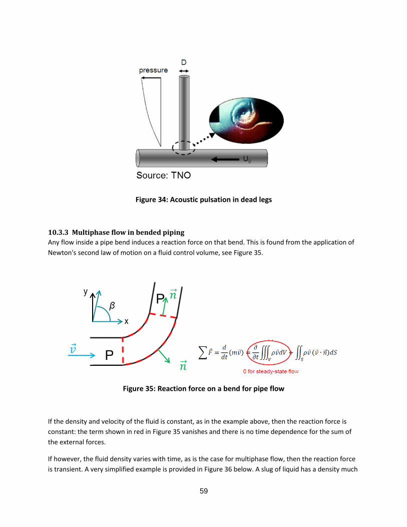
10.3.2 Acoustic pulsation in dead legs
Acoustic pulsations may also develop in sections of piping which are closed at one end and connected to
another pipe conveying dry gas at the other end, see Figure 34. As for the singing riser cavities, small
vortices will be shed at the upstream edge of the dead leg mouth, and collide with the downstream
edge. This produces a pressure perturbation which, if the frequency of vortex shedding matches one of
the acoustic frequencies of the dead leg, is amplified. The frequency of vortex shedding depends on the
flow velocity in the main pipe and diameter of the dead leg. The acoustic frequency of the dead leg
depends on its length and the speed of sound in the gas.
Compared to the singing riser, the issue is structural. If resonance occurs, large dynamic pressure
pulsations develop in the dead leg in the form of standing waves. Depending on the shape of the dead
leg piping and its eigenfrequencies, these pulsations may induce "shaking forces", leading to vibration
and potential fatigue issues.
59
Figure 34: Acoustic pulsation in dead legs
10.3.3 Multiphase flow in bended piping
Any flow inside a pipe bend induces a reaction force on that bend. This is found from the application of
Newton's second law of motion on a fluid control volume, see Figure 35.
Figure 35: Reaction force on a bend for pipe flow
If the density and velocity of the fluid is constant, as in the example above, then the reaction force is
constant: the term shown in red in Figure 35 vanishes and there is no time dependence for the sum of
the external forces.
If however, the fluid density varies with time, as is the case for multiphase flow, then the reaction force
is transient. A very simplified example is provided in Figure 36 below. A slug of liquid has a density much

60
higher than that of the gas phase which is present in front and behind the slug. As the slug changes
direction inside the bend, a reaction force is created, which is higher than the reaction force from the
gas flow. If slugs are passing at a regular time interval, typically of the order of 1 second, and the piping
section has an eigenfrequency around 1 Hz, resonance will occur and the piping will experience
significant levels of vibration.
Figure 36: Transient reaction force created by the passage of a slug
10.4 Analysis of Flow-Induced Vibrations For mechanical (structure and fluid) engineers, FIV is probably the most interesting phenomenon to
analyze. Guidelines exist to screen for a risk of fatigue failure, but they are extremely conservative. In
case a risk is identified, analyzes are usually conducted according to the following steps:
Modeling of the transient forces induced by the flow. This can be done in various ways, for
example by the use of Computational Fluid Dynamics (CFD) on multiphase flows
Application of those transient forces to a dynamic mechanical model of the system. This
requires modeling and analysis skills in structural mechanics.
Determination of the system response and cyclic stresses at the hot-spots (connection points for
the system, ref. Figure 31)
Fatigue analysis to determine the fatigue life of the system
A system will in general be considered as safe to operate if the fatigue life, i.e. the estimated time
before a failure occurs, is longer than the life of the field.
One particular aspect of FIV is that the flow excitation is broadband: contrary to VIV, flow excitation
does not occur at a single frequency, but over a wide range of frequencies. This means that there is
usually no possibility to avoid resonance by shifting the eigenfrequencies of the system outside the
range of flow excitation. In other words, resonance cannot be avoided.

61
11 Wax Wax is a class of hydrocarbons that are natural constituents of any crude oil and most gas condensates.
Waxy oils may create problems in oil production due to three main reasons:
Restricted flow due to reduced inner diameter in pipelines and increased wall roughness
Increased viscosity of the oil
Settling of wax in storage tanks
First, there is a potential for the wax to crystallize and adhere onto surfaces like the pipe wall in a
pipeline and thereby form a deposit layer which will increase with time and eventually, in the worst
case, completely block the line. Such deposition will reduce the capacity of the line by decreasing the
effective diameter and increasing the wall roughness and thus the pressure drop in turbulent flow. For
any pipeline experiencing wax deposition, there has to be a wax control strategy. Most often, the wax
control strategy simply consists of scraping the wax away from the pipe wall by regular pigging.
Sometimes, substantial quantities of wax are removed from the line. In one case several tons of wax was
collected in the pig trap at Statfjord B after pigging the line from Snorre B.
Figure 37: Part of wax plug retrieved from the pig trap at Statfjord B (sept 2001)
Secondly, wax precipitation causes the bulk viscosity of the oil to increase sharply and become shear-
rate dependent (non-Newtonian), leading to increased pressure losses. Ultimately, when a sufficient
amount of solid wax has precipitated (approximately 4-6 wt%), the wax tends to form a three-
dimensional network resulting in even larger viscosity increase ending up with a completely gelled

62
structure with solid-like mechanical properties. Particularly during production shut-downs, when the oil
is allowed to cool statically in the pipeline, this may be a severe situation, since high pressure may be
required to break down the gel structure upon restart. When performing regular pigging of a pipeline,
the internal diameter is maintained as no/little wax deposit is allowed to build up. This will ensure an
efficient flow.
Figure 38: Wax can deposit at inner walls if the temperature is below WAT
Figure 39: Manipulation of WAT by separation at different stages/temperatures.
The wax appearance temperature (WAT) in the gas phase can be manipulated through separation at
different stages/temperatures.

63
Table 3: U-value sensitivity to evaluate whether insulation can be used as wax control
Pipe size Tin [C] U-value [W/m2K] Pipe length @ 34C
8” 80 200 750 m
8” 80 50 3000 m
8” 80 3 52 km
8” 80 1 128 km
8” 60 200 500 m
8” 60 50 2000 m
8” 60 3 35 km
8” 40 200 150 m
8” 40 50 600 m
8” 40 3 10 km
The wax appearance temperature of most "normal", paraffin North Sea oils and condensates is in the
range 30° to 40°C.
Hot flushing or direct heating must be at a temperature at least 20°C above WAT (WDT Wax
Disappearance Temperature).

64
12 Erosion
12.1 Causes of erosion Erosion can be generated by a number of phenomena:
• Particulate erosion
– Solids produced
– Proppants used for gravel pack or fracking the reservoir
• Liquid droplet erosion
– Impingent of liquid droplets
• Cavitation
• Erosion corrosion
Particulate erosion by sand is most likely to cause erosive failures in oil and gas production systems.
12.1.1 Droplet erosion
Confined to wet gas and multiphase flows in which droplets can form. Droplet erosion occurs when
liquid droplets (or liquid jets) impinge at a surface at high speed.
The erosion rate is dependent on a number of factors including the droplet size, impact velocity, impact
frequency, and liquid and gas density and viscosity.
Test have shown solid-free erosion only occurs at very high velocities DNV-RP-O501 uses a velocity
above 70 – 80 m/s. Droplet erosion may be experienced at the leading edge turbines and potentially in
gas/mist flow in chokes.
The material loss is due to the impact of droplets at the material surface resulting in high pressure
pulses. The forces of droplet impact damage the material by formation of pits and cracks on the surface
and by loss of the material.

65
12.1.2 Cavitation
When liquid passes through a restriction low pressure areas can be generated. If the pressure is reduced
below the vapor pressure of the liquid, bubbles are formed. These bubbles then collapse generating
shock waves. These shock waves can be of sufficient amplitude to damage pipework.
The collapse of vapor bubbles may result in loud noise, vibrations and erosion.
If the collapse occurs on a wall/material surface, a micro jet of liquid is formed and will be impacting on
the surface. This will create a high pressure pulse
Cavitation occurs rarely in oil and gas production systems as the operating pressures are well above
vapor pressure, but can be seen in chokes, control valves and pump impellers.
12.1.3 Erosion corrosion
Erosion-corrosion is the combined effect of particulate erosion and corrosion.
The progression of the erosion-corrosion process depends on the balance between the erosion and
corrosion processes:
In a purely corrosive flow new pipework components typically corrode very rapidly until a brittle
scale develops on the surfaces exposed to the fluid. This scale layer forms a barrier between the
metal and the fluid that substantially reduces the penetration rate.
In highly erosive flows, in which corrosion is also occurring, the erosion process predominates
and scale is scoured from exposed surfaces before it can influence the penetration rate.
At intermediate conditions erosion and corrosion mechanisms can interact. In this case scale can
form and then be periodically removed by the erosive particles.
12.1.4 Sand production and erosion due to produced sand
Erosion is due to impact of solid/sand particles at a surface. New wells typically produce a large amount
of sand and proppant as they “clean up”. Sand production then stabilizes at a relatively low level before
increasing again as the well ages and the reservoir formation deteriorates. Sand concentration typically
ranges from 1 to 50 parts per million by mass.
Gas systems generally has higher velocities than liquid systems; making them more prone to erosion.
However oil fields may have a higher concentration of produced sand.
Main concerns to be handled and planned for are:

66
Erosion due to sand production
Transportation of sand; avoid accumulation of sand in flowlines or subsea separators.
Particle trajectories in an elbow
a) Small particles b) Medium particles
(liquid system)
c) Large particle
(gas system)
Drag forces on sand particles are different in liquids and gases. Erosion rates in gas flows are usually
greater than in liquid flows operating at the same velocities. Also, the erosion scar position will be
different.
12.1.4.1 Impact erosion model
Consider Figure 23 depicting solid particles in a fluid flow traveling at a particle velocity of 𝑉𝑝 and
impacting a solid wall at an angle α.

67
Figure 40: Solid particles impacting on wall
Most erosion models for predicting erosive material loss for the wall are on the following form:
𝐸 = 𝐴𝑉𝑝𝑛 𝐹(𝛼)
Equation 63
Here
𝐸 is the erosion rate (kg of material removed/kg of erodant )
𝑉𝑝 is the particle impact velocity
𝐴 is a constant depending on the material being eroded and other factors
𝛼 is the particle impact angle
𝐹(𝛼) is a material dependent function of the impact angle between 0 and 1
𝑛 is a material dependent index
Note that material loss is proportional with the amount of solids/sand impacting on a surface provided
the sand concentration is not too high; i.e. typically <1-5% by volume.
12.1.4.2 Guidelines and sand erosion prediction methods
The recommended practice DNV-RP-O501 – Erosive Wear in Piping Systems is widely used as a guideline
and for predicting erosion due to sand production is subsea production systems. The recommended

68
practice includes an impact erosion model and empirical models for calculating erosion in common
piping components such as:
- Straight pipes
- Welded joints
- Reducers
- Elbows
- Blind tees
- Intrusive sand sensors
For multiphase flow, DNV uses mixture velocities and mixture density and viscosity as input to the
flow/particle calculations. These empirical models have proved useful in estimating erosion due to sand
production and aiding in the design and line sizing of subsea systems.
Another often used guideline is the API 14E although it is widely accepted to be misleading and
incorrect. The API 14E standard does not account for the physical phenomena governing the erosion
process. Note also that the recommendations given in API 14E are highly conservative for liquid flows
and under-estimate the potential for erosion in gas flows.
For complex geometries or if more detailed analysis is required, CFD is required to determine the
particle trajectories and particle impact characteristics. Contribution to local pipe wall erosion is
calculated by adding up contributions for each particle impact on the wall using the DNV GL particle
erosion impact model:
�� = 𝐾 ∙ 𝑚 ∙ 𝑉𝑝𝑛 𝐹(𝛼)
Equation 64
Mass of particles impacting on the surface is denoted 𝑚 and the resulting wall material loss is denoted
��.The material grade is characterized by the material constant 𝐾 and 𝑛 and a material response
function 𝐹(𝛼). The material parameters are determined by testing.
The shape of the material function 𝐹(𝛼) depends on the type of group for used. Figure 24 shows 𝐹(𝛼)
for both ductile materials (steel) and brittle materials respectively. For ductile materials, e.g. steel
grades, the most critical erosion is obtained at impact angle in the range 25-40°. For brittle materials;
e.g. ceramics or WC materials, the most critical impact angle is close to 90°. The difference in most

69
critical impact angle for ductile and brittle materials is reflecting the difference in erosion mechanisms.
Material removal/erosion for ductile materials are due to mechanical action, while for brittle materials
the removal of material/erosion is due to brittle fracture due to repeated impact at the material surface.
Figure 41: Material function F(α) for ductile and brittle materials
For steel grades DNV uses K = 2 E-9 (m/s)-n and n=2.6. It is documented experimentally that the erosion
characteristics/resistance is more or less the same all standard steel grades. For wolfram carbide (brittle
material) K=1.1E-10 to 3.2E-10 (m/s)-n depending of type and n = 2.2.
The DNV GL erosion models are developed based on tests with angular particles representative for
particles produced in the North Sea. Erosion is dependent on the shape of the particles; i.e. the erosion
rate increases with the angularity. Sharp/very angular particles may typically give 2-3 the erosion rate as
for angular particles, while rounded particles may give 2-3 times less erosion than angular particles.
Figure 42: Erosion wear in complex geometries

70
13 Overview simulation models in flow assurance It is important to understand the difference of the suitability for the different simulation models. For
transient multiphase models there exists a hierarchical regime of models. A rule of thumb is to start
with the simplest model in steady state modus, i.e. HYSYS steady state, FlowManagerTM, OLGA steady
state and gradually increase the physical complexity of the problem by use of more complex models i.e.
HYSYS dynamics and OLGA transient. The last phase of complexity is the CFD analysis which should
never be used before a crucial mapping of need has been performed as this is a very detailed activity
and needs to be used in combination with the other ones.
In the same manner the erosion analysis should start with a simple screening by the DNV erosion model
RP 0501 or FlowManagerTM, erosion model. The potential problem areas that have been identified will
then be investigated by use of CFD. In the thermal analysis only an analytical approach is available for
the first screening. The main calculations need to be done by FEA and in some cases a more refined CFD
is required.
For the analysis and calculation regarding fluid properties, i.e. hydrate strategy and wax strategy, the
simulation tool to be used is PVTsim. In PVTsim a whole specter of equations of state is available. In the
Marlim project the Penelux Peng Robinson equation of state has been used for fluid property analysis.
Table 4: Overview simulation models that are used in flow assurance
Simulation model Purpose Output
FlowManagerTM Multiphase design
Steady state
Quick pressure-temperature-
flow rate analysis of long flow
lines
Pressure
Temperature
Flow Rates
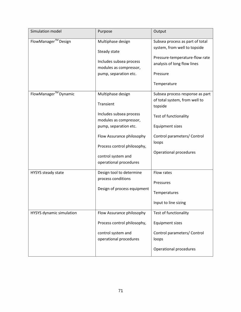
71
Simulation model Purpose Output
FlowManagerTM Design Multiphase design
Steady state
Includes subsea process
modules as compressor,
pump, separation etc.
Subsea process as part of total
system, from well to topside
Pressure-temperature-flow rate
analysis of long flow lines
Pressure
Temperature
FlowManagerTM Dynamic Multiphase design
Transient
Includes subsea process
modules as compressor,
pump, separation etc.
Flow Assurance philosophy
Process control philosophy,
control system and
operational procedures
Subsea process response as part
of total system, from well to
topside
Test of functionality
Equipment sizes
Control parameters/ Control
loops
Operational procedures
HYSYS steady state Design tool to determine
process conditions
Design of process equipment
Flow rates
Pressures
Temperatures
Input to line sizing
HYSYS dynamic simulation Flow Assurance philosophy
Process control philosophy,
control system and
operational procedures
Test of functionality
Equipment sizes
Control parameters/ Control
loops
Operational procedures

72
Simulation model Purpose Output
PVTsim Fluid properties analysis
Hydrate curve
Fluid properties tables for
simulation models
Hydrate curves
Wax appearance
Composition of multiphase
fluids
Phase envelope
RP O501 DNV Erosion calculations Screening of erosion rates
Map potential problem areas
CFD multiphase Detailed erosion analysis
Detailed analysis of erosion hot-
spots
CFD/FEA Thermal analysis
Detailed analysis of cold-spots
OLGA steady state multiphase Multiphase design
Steady state
Pressure-temperature-flow rate
analysis of long flow lines
Pressure
Temperature
Flow rates
Flow regime
OLGA transient multiphase Multiphase design
Flow regime
Slug tracking
Slug volume
CFD transient multiphase Multiphase design
CFX
Details of flow behavior

73
14 Field developments - Concept Selection In this part different field developments will be investigated with examples from existing system
designs. The target is to give an understanding of how a flow assurance engineer will work to assure the
field.
14.1 Types of fields Table 5: Types of fields
Types of fields Types/Concept Typical Flow Assurance Challenges and
solutions for specific fields
New fields
Unique
combination of
fluid properties,
pressure,
temperature,
topography and
field layout
combination
Normal
accessible fields
Gas Hydrate management
Wax Management
Erosion (Velocity)
Flow Induced Vibrations
Oil Hydrate management
Wax management
Difficult
accessible fields
Very deep
water and/or
reservoirs
Boosting requirements
Hydrate
Wax
Long tie-ins Pressure drop
Hydrate
Wax
Heavy oil with
low API°(high
viscosity, high
spec gravity)
Hydrate
Wax
Asphaltenes, scale
Temperature
High pressure drop

74
Types of fields Types/Concept Typical Flow Assurance Challenges and
solutions for specific fields
Examples Boosting and separation (Pazflor)
Separation (Troll)
High
pressure/high
temperature
Typically gas Material temperature limits (subsea
cooling)
Operate between hydrate /WATand high
limit
Old fields
Tail-end
production
Increased
Oil/Gas recovery
with boosting
Dry Gas
compression
(Subsea
compression,
liquid pump,
separator)
Åsgard
Ormen Lange
Wet Gas
compression
Gullfaks
Multiphase
Pump
Water prod Hydrate
Scale
Separation Tordis (North sea)
Marlim (Brazil)
* All fields are unique which means that the combination of fluid properties, pressures and
temperatures and field layout must be evaluated for each new field
14.2 Floater/Subsea At the time being the subsea concepts very often competes with a more traditional floater solution.
For shallow water depths, bottom-founded facilities like jack up drilling rigs and fixed offshore structures
can be used, and where saturation diving is feasible.
Recently, all subsea solutions are also considered in shallow water fields as they can compete with
floating platforms in cost and reliability.

75
Figure 43: Concepts of floating or fixed constructions

76
Figure 44: Active GulfOil rigs
Figure 45: All subsea, vision of topside-less field developments

77
15 Examples of field developments with subsea process stations
15.1 Troll Pilot - liquid/liquid separation
With its 115 subsea wells Troll is the largest subsea development in the world. The wells are
characterized by their production from thin oil zones which has required the development of new
drilling and completion technology (1995).
Troll pilot started production in the Troll field in 2001. It was the first subsea separation system to be
installed on the sea bed at 340 meters and 3.5 km from the platform.
By means of the gravity method produced water is separated from the oil and gas flow from four of Troll
C's producing wells. The water is then injected back into the reservoir, while the separated oil and gas
are sent up to the platform.

78
The Troll C subsea separation system is tied back 3.3 km to the Troll C platform in 350 m of water. The
subsea station makes it possible to separate water from the well stream on the seafloor and re-inject it
into a low-pressure aquifer so that the water does not have to be transported back to the main
platform. Eight wells can be routed through the processing station, which is designed to process four
wells at a time, provided they are at normal production rates.
The main processing modules are the horizontal gravity-based separation vessel and the subsea water
re-injection pump. A fully automated control system with separation level instrumentation and variable
speed drive system provides the main functional blocks for control of the process system.
The well stream is routed into the separator from one of the main production lines. Pre-processing is
done in an innovative inlet mechanism called a low-shear de-gassing device. Its purpose is to split the
gas and liquids to reduce the speed of the liquids and limit the emulsion formed. Once past the inlet
device, the liquid is allowed to settle in the separator vessel, and the separated water is taken out
directly to the water re-injection pump. From there, the oil and gas is commingled and forced back to
the Troll C semi by the flowing pressure in the separator and pipeline system. The separated produced

79
water is re-injected into the disposal reservoir by the subsea water injection pump via a dedicated
injection well.
Depth: 340 m, Step-out: 600 m, Design pressure: 179 bar, Design temperature: -5-68 °C, Operation
pressure: 16-40 bar, Operation temperature: 40-60 °C
Figure 46: Troll Pilot
Troll B features liquid/liquid separation (water from oil), re-injection of water and
multiphase boosting of oil and gas. The separator used is the Pipe Separator developed by Hydro.
15.2 Tordis Located in the Tampen area west of Bergen Tordis came on stream in 1994. After many years of
operation the energy (pressure) in the reservoir has dropped and in addition the water content in the
produced liquid has increased.
The reduced energy is thus used for transporting great volumes of superfluous liquid.
Typical challenges for mature subsea oil fields are increased water cut which has the following
consequences:
Increased hydrostatic head towards platform
o Reduced production

80
o Not possible to restart wells
Need for increased capacity on platform water treatment facilities
Need for increased amounts of Methanol/MEG for hydrate prevention
o Need for expensive modifications
o Limitations in infra structure
Increased oil recovery from Tordis field increased the recovery from 49% to 55% which added 35 million
barrels of oil reserves.
Figure 47: Tordis field layout
Figure 48: Tordis subsea separation station

81
Figure 49: System overview
Water and sand are separated from the well stream close to the reservoir and injected into a subsea
formation for storage.
In addition a multi-phase pump helps send oil and gas through a 10-kilometre pipeline to Gullfaks C for
processing, storage and export.
Optimizing the use of energy, this solution is also environmentally friendly as it reduces the volume of
produced water discharged into the sea.
15.3 Pazflor - Gas/Liquid Separation and Liquid Boosting

82

83
Gas / Liquid Separation and Liquid Boosting:
Gas flows freely to the FPSO
Hydrate preventions of flowlines by means of depressurization is possible
Reduced cost due to elimination of circular flow line
Liquid out of separator with relative low GVF
Efficient pumps with high ∆P can be used → Increased recovery & less power consumption
Boosting of liquid
Stabilized flow regime in risers → reduced slugging
15.4 Marlim Mature field, in operation since 1991

84
Subsea separation in a deepwater, mature field environment
Reinjection of water into production reservoir
Separation of heavy oil in a subsea environment

85
16 Vocabulary Abbreviation Definition
ASV Anti Surge Valve
Bar Unity of pressure equal to 100kPa roughly the atmospheric pressure at sea-
level
Bara Absolute pressure ref to vacuum
Barg Pressure above 1 atmosphere
BHP Bottom Hole Pressure
CFD Computational Fluid Dynamics, both Fluent and CFX are simulation packages
for CFD (solution of the full Navier-Stokes equations, nonlinear and
dynamic)
CFD Computational Fluid Dynamics
Company Petrobras
Company StatoilHydro
Conceptual Design Early phase design/ Study
CP Cathodic Protection
DNV Det Norske Veritas
dP Differential Pressure
EPC Engineering Procurement Construction (Contract)
ESD Emergency Shut Down
FEA Finite Element Analysis (computer-based numerical technique for obtaining
near-accurate solutions to a wide variety of complex engineering problems
where the variables are related by sets of algebraic, differential, and integral
equations)
FEED Front End Engineering Design
FIV Flow Induced Vibrations
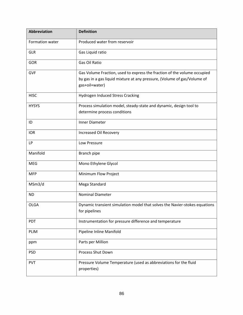
86
Abbreviation Definition
Formation water Produced water from reservoir
GLR Gas Liquid ratio
GOR Gas Oil Ratio
GVF Gas Volume Fraction, used to express the fraction of the volume occupied
by gas in a gas liquid mixture at any pressure, (Volume of gas/Volume of
gas+oil+water)
HISC Hydrogen Induced Stress Cracking
HYSYS Process simulation model, steady-state and dynamic, design tool to
determine process conditions
ID Inner Diameter
IOR Increased Oil Recovery
LP Low Pressure
Manifold Branch pipe
MEG Mono Ethylene Glycol
MFP Minimum Flow Project
MSm3/d Mega Standard
ND Nominal Diameter
OLGA Dynamic transient simulation model that solves the Navier-stokes equations
for pipelines
PDT Instrumentation for pressure difference and temperature
PLIM Pipeline Inline Manifold
ppm Parts per Million
PSD Process Shut Down
PVT Pressure Volume Temperature (used as abbreviations for the fluid
properties)

87
Abbreviation Definition
ROV Remote Operated Vehicle
SCM Subsea Control Module (Control Pod)
SCS(t) Subsea Compression Station
Slug Liquid volume in multiphase flow
Slug Catcher Liquid catcher
SPS Subsea Process System/Subsea Production System
SSAO Submarine Oil/water Separation System
SSBS Subsea boosting station
Standard Defined according to 1bar, 15(20)°C
Surge Mix of gas and liquid
Template Several wells put together on one frame, well cluster
THP Top Hole Pressure
TQP Technical Qualification Program
UPS Un-interruptible Power Supply
UTA Umbilical Termination Assembly
VCM Vertical Connector Module
Vol% Volume percentage
VSD Variable Speed Drive
WC Water Cut, fraction of water in total liquid
WI Water Injection
WSIP Well Shut In Pressure
Wt weight
yr Year

88
17 Literature [1] PipeFlow 1 and 2, Ove Bratland, free on net
[2] NORSOK standard P-001, Process design, free on net
[3] Innføring I fluidmekanikk, UiO, Bjørn Gjevik
[4] An introduction to multiphase flow, UiO, Ruben Schulkes
[5] Applied fluid dynamics handbook, Blevins, Krieger
[6] Guidelines for the Avoidance of Vibration Induced Failure in Process Pipework.
[7] Water content of gas, chart, attached
[8] Hydraulics of pipeline systems, B.E. Larock, R.W. Jeppson and G.Z. Watters, CRC Press, 2000

89
18 Attachments
18.1 Water content in natural gas