flow and heat transfer in a turbocharger radial turbine1055646/fulltext01.pdf · flow and heat...
TRANSCRIPT

Flow and heat transfer in a turbocharger radialturbine
by
Shyang Maw Lim
December 2016Technical Reports from
Royal Institute of TechnologyKTH Mechanics
SE-100 44 Stockholm, Sweden

Akademisk avhandling som med tillstand av Kungliga Tekniska Hogskolan iStockholm framlagges till offentlig granskning for avlaggande av teknologielicenciatexamen torsdag den 19 januari 2017 kl 13:15 i sal Q2, Osquldasvag 10,Kungliga Tekniska Hogskolan, Stockholm.
TRITA-MEK Technical report 2016:19ISSN 0348-467XISRN KTH/MEK/TR-16/19-SEISBN 978-91-7729-238-8
c©Shyang Maw Lim 2016
Universitetsservice US–AB, Stockholm 2016

Shyang Maw Lim 2016, Flow and heat transfer in a turbocharger radialturbine
Competence Center for Gas Exchange (CCGEx) andLinne Flow Centre, KTH Mechanics, SE-100 44 Stockholm, Sweden.
AbstractIn the past decades, stricter legislation has been imposed to improve fuel econ-omy and to reduce tail-end emissions of automotive vehicles worldwide. Oneof the important and effective technologies adopted by the automobile manu-facturers to fulfill legislation requirements is the turbocharger technology. Asunavoidable large temperature gradients exists in an automotive turbocharger,heat transfer is prominent. However, the effects of heat loss on the turbochargerturbine performance is unclear, i.e. there is no consensus about its effectsamong researchers. Therefore, the objective of the licentiate thesis is to inves-tigate the effects of heat transfer on an automotive turbocharger radial turbineperformance. Furthermore, the thesis also aims to quantify the heat trans-fer related losses in a turbocharger turbine. Both gas stand (continuous flow)and engine-like (pulsating flow) conditions are considered. By using DetachedEddy Simulation (DES), the flow field of the targeted turbocharger turbine iscomputed under adiabatic and non-adiabatic conditions. Energy balance andexergy concept are then applied to the simulations data to study the effects ofheat loss on performance and to quantify the heat transfer related losses. Themain findings of the licentiate thesis are 1) Pressure ratio drop in turbine isless sensitive to heat loss as compared with turbine power, and hence there is arisk of making wrong conclusions about the heat transfer effects on the turbineperformance by just comparing the measured pressure ratio under adiabaticand non-adiabatic scenarios; 2) It is possible to quantify heat transfer relatedlosses in a turbocharger turbine. This quantification allows understanding onhow well the turbine system utilizes the available energy, and assisting identifi-cation of the system component that is sensitive to heat transfer; 3) Heat losshas insignificant effect on turbine power under the investigated engine-like pul-sating flow condition; and 4) Even under unavoidable non-adiabatic conditions,much of the exergy is discharged to the environment and more effort could bedone to recover the wasted exergy as useful work in the current turbine system.The outcomes of the licentiate thesis naturally lead to the main focus of futurework, i.e. exploring different exhaust valve strategies to minimize losses and tooptimize flow exergy extraction as useful turbine work for better exhaust gasexergy utilization.
Descriptors: pulsatile exhaust flow, efficient radial turbine, turbocharger per-formance, Detached Eddy Simulation, level of integration with the InternalCombustion Engine, heat transfer effect
iii

Shyang Maw Lim 2016, Stromning och varmeoverforing i en turbolad-dare med radialturbin
Competence Center for Gas Exchange (CCGEx) andLinne Flow Centre , KTH Mekanik , SE - 100 44 Stockholm , Sverige.
Sammanfattning Under de senaste decennierna har allt strangare lags-tiftning inforts for att forbattra bransleekonomin och minska avgasutslappenfran motorfordon varlden over. En av de viktigaste och mest effektiva teknikersom inforts av biltillverkarna for att kunna uppfylla lagkraven ar turbolad-dartekniken. Eftersom stora temperaturgradienter existerar i en fordonsturbo-laddare, spelar varmeoverforing en framtradande roll. Emellertid ar effekternaav varmeforluster pa turboturbinprestanda oklar, dvs det finns ingen konsen-sus bland forskare om dess effekter. Syftet med denna licentiatavhandling ardarfor att undersoka effekterna av varmeoverforing pa prestanda for radial-turbinen i en fordonsturboladdare. Vidare syftar avhandlingen till att kvan-tifiera varmeoverforingsrelaterade forluster i en turboladdares turbin. Badefall med kontinuerligt gas flode och motorliknande, pulserande flode beak-tas. Stromningsfaltet i den utvalda turboladdarens turbin beraknas med enmetod kallad Detached Eddy Simulation (DES) under adiabatiska och ickeadiabatiska forhallanden. Energi- och exergibalanser for simuleringsresultatenanalyseras sedan for att studera effekterna av varmeforluster pa prestanda ochkvantifiera varmeoverforingsrelaterade forluster. De viktigaste resultaten avlicentiatuppsatsen ar 1) Tryckforhallandet over turbinen ar mindre kansligt forvarmeforluster jamfort med turbineffekten. Darmed finns det en risk for attfelaktiga slutsatser dras betraffande effekterna av varmeoverforing pa turbin-prestanda genom att enbart jamfora det uppmatta tryckforhallandet underadiabatiska och icke adiabatiska forhallanden; 2) Det ar mojligt att kvantifieravarmeoverforingsrelaterade forluster i en turboladdares turbin. Denna kvan-tifiering ger forstaelse for hur val turbinsystemet utnyttjar den tillgangligaenergin, och bistar med identifiering av systemkomponenter som ar kansligafor varmeoverforing; 3) Varmeforluster har en obetydlig inverkan pa turbin-effekten for det undersokta motorliknande, pulserande flodesforhallandet; och4) Under oundvikliga, icke-adiabatiska forhallanden, slapps aven en stor del avexergin ut till omgivningen och det finns utrymme for forbattringar gallandeexergiutnyttjandet i det aktuella turbinsystemet. Baserat pa resultaten av li-centiatavhandlingen kommer det fortsatta arbetet att fokusera pa att utforskaolika avgasventilstrategier for att minimera forluster och optimera omvandlingav flodesexergi till anvandbart turbinarbete for battre avgasexergiutnyttjande.
Deskriptorer: pulserande avgasflode, effektiv radialturbin, turboaggregatpre-standa, Detached Eddy Simulation, integrationsniva med forbranningsmotorn,varmeoverforingseffekt
iv
Preface
This licentiate thesis represents an effort to improve the understanding of heattransfer and heat transfer related losses of a turbocharger turbine. The the-sis is a monograph, which consists of a total of seven chapters. Chapter Onebriefly describes the needs and working principle of turbocharging and definesthe research scopes and objectives of the thesis. Chapter Two discusses theimplications of heat transfer on turbine performance, reviews current state-of-the-arts and defines the performance metrics used in describing the turbineperformance. Descriptions about turbulence models and numerical methodsused in this study are summarized in Chapter Three and Four, respectively.In Chapter Five, validation and verification of the computational setup is ad-dressed. Chapter Six reports the main results of the thesis, in which the effectsof heat transfer on turbine performance under hot gas stand (continuous flow)and engine-like (pulsating flow) conditions are discussed. Proposed future workcan be found in the last chapter of the thesis, i.e. Chapter Seven. I would appre-tiate comments and suggestions from both academia and industry to enhancethe study analysis, to deepen the interpretation of the results, and to improvethe readability of the thesis. Thank you and I hope that you enjoy reading thethesis.
December 2016, Stockholm
Shyang Maw Lim
v

Quality is much better than quantity. One home run ismuch better than doubles.
Steve Jobs (1955–2011)
vi
Contents
Abstract iii
Preface v
Chapter 1. Introduction 1
1.1. Global standards on fuel economy and emissions 1
1.2. Supercharging and turbocharging 2
1.3. Heat transfer in turbochargers 8
1.4. General effects on performance 10
1.5. Research scopes and objectives 12
Chapter 2. Turbine and turbine performance metrics 15
2.1. Heat transfer implications on turbocharging 15
2.2. Modeling of heat transfer 17
2.3. Turbocharger performance and assessment 20
2.4. Turbine power and torque 26
2.5. Heat transfer rate 27
2.6. Exergy analysis 27
2.7. Bejan number 29
Chapter 3. Turbine flow modeling 30
3.1. Compressible flow governing equations 30
3.2. Reynolds Averaged Navier-Stokes (RANS) modeling 32
3.3. Large Eddy Simulation (LES) modeling 35
3.4. Detached Eddy Simulation (DES) modeling 37
Chapter 4. Numerical methods 39
4.1. Discretization 39
4.2. Boundary conditions 41
vii

Chapter 5. Method of validation and verification 44
5.1. Computational domain and grid 44
5.2. Boundary conditions 45
5.3. Methodology 46
5.4. Grid convergence study 47
5.5. Influence of turbine wheel rotation per time-step 54
5.6. Stationary-rotating interface type sensitivity 55
5.7. Influence of turbulence model 64
Chapter 6. Heat transfer effects on the turbine performance 70
6.1. Turbine assessment under continuous flow conditions 70
6.2. Exhaust manifolds and pulsating flow effects 74
Chapter 7. Summary and future work 82
Acknowledgements 84
References 86
viii

CHAPTER 1
Introduction
Turbocharging has been proposed and invented more than 100 years ago byAlfred Buchi in 1905, but extensive development and application of the tech-nology in automotive vehicles have only been started about 30 years ago (seee.g. Ninkovic 2014; Watson & Janota 1982). The popularity of turbocharging inautomotive vehicle is mainly driven by stricter legislation in fuel consumptionand tail-end emissions introduced since 1980s (Ninkovic 2014). This chapterstarts with an overview of the trend of global standards on fuel economy andemissions, and discusses the near future prospects of turbocharging. It followsby a brief explanations about the working principle of turbocharging and iden-tification of heat transfer issues in turbocharging. Finaly, the chapter endswith the definition of research scopes and objectives of this licentiate thesis.
1.1. Global standards on fuel economy and emissions
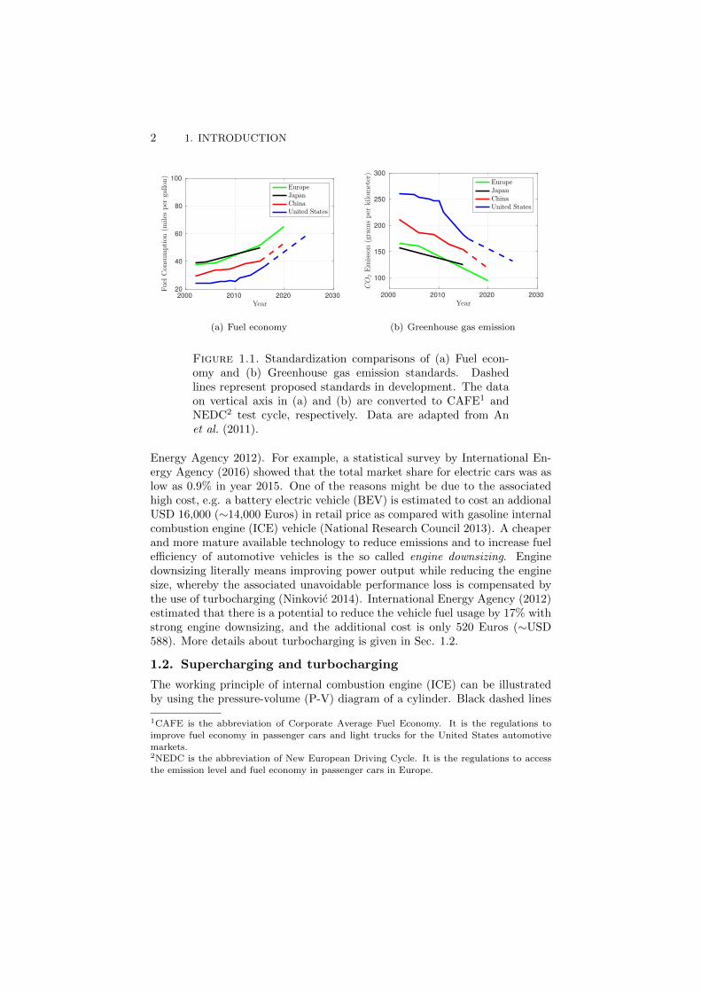
In the past decades, stricter legislation has been imposed to improve fuel econ-omy and to reduce tail-end emissions of automotive vehicles worldwide. Asan example, Fig. 1.1(a) compares the fuel economy legislation standard be-tween four major automobile markets, i.e. the United States (US), EuropeanUnion (EU), Japan and China. Although the standard varies among countriesin terms of target and implementation timeline, it is obvious that the overalltrend is moving towards more efficient usage of fuel in automotive vehicles,i.e. travel greater distance with less fuel. As for greenhouse gases, it can beobserved from Fig. 1.1(b) that every region is working towards lower emissionslevel. Note that there is a sharp change in the fuel economy and greenhousegas emission standards at year 2005 (especially Europe), which indicates thestarting point of stricter environmental policies implementation. Therefore, itis crucial that automobile manufactures constantly seek for innovative tech-nologies to improve fuel economy and to reduce air pollutant emissions as tofulfill the legislation requirements.
Currently, there is an extensive range of competence technologies availablefor improving fuel economy and reducing greenhouse gas emissions of automo-tive vehicles. Although most of the technologies are available commercially,some of them have difficulty to secure satisfactory market share (International
1
2 1. INTRODUCTION
2000 2010 2020 2030
Year
20
40
60
80
100
Fuel
Con
sumption
(miles
per
gallon
)
EuropeJapanChinaUnited States
(a) Fuel economy
2000 2010 2020 2030
Year
100
150
200
250
300
CO
2Emisson(gramsper
kilom
eter)
EuropeJapanChinaUnited States
(b) Greenhouse gas emission
Figure 1.1. Standardization comparisons of (a) Fuel econ-omy and (b) Greenhouse gas emission standards. Dashedlines represent proposed standards in development. The dataon vertical axis in (a) and (b) are converted to CAFE1 andNEDC2 test cycle, respectively. Data are adapted from Anet al. (2011).
Energy Agency 2012). For example, a statistical survey by International En-ergy Agency (2016) showed that the total market share for electric cars was aslow as 0.9% in year 2015. One of the reasons might be due to the associatedhigh cost, e.g. a battery electric vehicle (BEV) is estimated to cost an addionalUSD 16,000 (∼14,000 Euros) in retail price as compared with gasoline internalcombustion engine (ICE) vehicle (National Research Council 2013). A cheaperand more mature available technology to reduce emissions and to increase fuelefficiency of automotive vehicles is the so called engine downsizing. Enginedownsizing literally means improving power output while reducing the enginesize, whereby the associated unavoidable performance loss is compensated bythe use of turbocharging (Ninkovic 2014). International Energy Agency (2012)estimated that there is a potential to reduce the vehicle fuel usage by 17% withstrong engine downsizing, and the additional cost is only 520 Euros (∼USD588). More details about turbocharging is given in Sec. 1.2.
1.2. Supercharging and turbocharging
The working principle of internal combustion engine (ICE) can be illustratedby using the pressure-volume (P-V) diagram of a cylinder. Black dashed lines
1CAFE is the abbreviation of Corporate Average Fuel Economy. It is the regulations toimprove fuel economy in passenger cars and light trucks for the United States automotivemarkets.2NEDC is the abbreviation of New European Driving Cycle. It is the regulations to access
the emission level and fuel economy in passenger cars in Europe.
1.2. SUPERCHARGING AND TURBOCHARGING 3
in Fig. 1.2 shows an ideal dual-combustion cycle of a naturally aspirated en-gine. At point 1, the piston is at bottom dead center (BDC) and it denotesthe beginning of compression stroke. From point 1 to 2, the air-fuel mix-ture in the cylinder undergoes continuous compression. The air-fuel mixtureis then ignited with electric spark plug (spark ignition SI) or self-ignited dueto high temperature after compression (compression ignition CI). This com-bustion process happens instanteneously at constant volume from point 2 to3 at top dead center (TDC) position. The remaining part of the combustionoccurs at constant pressure from point 3 to 4, where the hot gases push thepiston downward (increasing volume) along the cylinder. The gases are thenexpanded continously from point 4 to 5. At point 5, the exhaust valve opensand gas leaves the cylinder. This causes the pressure in the cylinder falls backto the ambient condition. The net work output per cycle is the area enclosedby the envelope of the P-V diagram (area 1-2-3-4-5-1) and it is converted tousable work to propel the vehicle through a series of mechanical systems.
It can be seen from Fig. 1.2 that pressure depends on the process path.It is more convenience to represent the pressure by a corresponded path inde-pendent average pressure. This average pressure is independent on the pistondisplacement and it is known as Indicated Mean Effective Pressure (IMEP)pmi (see Fig. 1.2). Due to the fact that not all of the net work output canbe converted to usable work to move the vehicle, friction (represented by Fric-tional Mean Effective Pressure pmf ) must be deducted from pmi and the cor-responded average pressure is known as Brake Mean Effective Pressure pme.The relationships among pmi, pmf and pme can be expressed by Eq. 1.1. Agraphical representation to describe the relationships is illustrated in Fig. 1.3.
pme = pmi − pmf . (1.1)
The engine power output Wengine in Watt is given by
Wengine = C · nengine · pme · Vsw , (1.2)
where nengine is the engine speed in revolution per second (rps), pme is theBrake Mean Effective Pressure in N/m2 and Vsw is the swept cylinder volumein m3. C is a dimensionless constant depending on the engine type, i.e. 1 fortwo-stroke engine and 1/2 for four-stroke engine.
From Eq. 1.2, it is clear that engine power Wengine can ben increased bythe following methods.
1. Increasing the swept cylinder volume Vsw.

4 1. INTRODUCTION
P
V
4
4'3' 3
2'2
55'
1 1'
pmi
Maximum
pressure
Ambient
pressure
Boost
pressure
VswV'sw
Solid line: Supercharging
Dashed line: Naturally
aspirated
Figure 1.2. Comparisons of the P-V diagram of super-charged and naturally aspirated standard dual-combustion cy-cle having the same maximum pressure but different compres-sion ratio. Vsw is the swept cylinder volume. Adapted fromWatson & Janota (1982).
2. Running the engine at higher engine speed nengine.
3. Increasing the brake mean effective pressure pme.
Method (1) has the disadvantage of increasing engine size, and this leadsto an increment in engine weight and higher frictional losses. Method (2) isalso unfavorable because frictional losses increase with engine speed nengine.This means that the brake mean effective pressure pme is lower and ultimatelythe engine power output Wengine is being reduced (see Eq. 1.2). Therefore, in
order to increase the engine power Wengine, it is crucial to increase the brakemean effective pressure pme, while keeping the swept cylinder volume Vsw andthe engine speed nengine low. The brake mean effective pressure pme can beincreased by introducing air at density greater than the atmospheric conditioninto an engine. This method is known as supercharging, as defined in Watson &

1.2. SUPERCHARGING AND TURBOCHARGING 5
P
V
pme
pmi
pmf
Vsw
Figure 1.3. Graphical illustration to describe the relation-ships among Indicated Mean Effective Pressure pmi, FrictionalMean Effective Pressure pmf and Brake Mean Effective Pres-sure pme in a P-V diagram. Vsw is the swept cylinder volume.
Janota (1982). The merits of supercharging can be seen from Fig. 1.2, whichcompares the P-V diagram of a naturally aspirated (black dashed line) andideal supercharged (black solid line) cycle. From Fig. 1.2, it is clear that the
starting point of supercharged cycle 1′
is at higher pressure than the ambientcondition. This means that air with higher density is used for combustionand the net work output (area of envelop 1
′-2′-3′-4′-5′-1′) is greater than the
naturally aspirated engine (area of envelop 1-2-3-4-5-1).
In order to achieve higher air density at point 1′, a compressor is used to
increase the air pressure above ambient level. This can be achieved via (1)mechanical supercharging and (2) turbocharging. In mechanical superchaging,the required compressor’s work is extracted from the crank shaft of the en-gine, as shown in Fig. 1.4. This implies that a portion of the engine powerWengine is used to drive the supercharging compressor. On the other hand, inturbocharging, highly energetic hot exhaust gases from engine combustion areused to drive a turbine, as illustrated in Fig. 1.5. As can be seen from Fig. 1.5also, the turbine is then used to spin a compressor, which is mounted on thesame shaft. Note that in turbocharging, the otherwise wasted exhaust gasesare ultilized and no engine power Wengine is consumed to drive the compres-sor. This makes turbocharging a more preferable option, as compared withmechanical supercharging.

6 1. INTRODUCTION
Inlet manifold
Power
Exhaust
gas owing outAmbient
air owing in
Chain, belt
or gear drive
Compressor
Figure 1.4. Typical arrangement of an engine fitted with amechanically driven supercharger. Adapted from Watson &Janota (1982).
Ambient
air in
Compressed
air out
Exhaust
gases in
Exhaust
gases out
Intake valve
Exhaust
valve
Charged
air cooler
Engine
cylinder
TurbineCompressorShaft
Engine
piston
Engine
crank
shaft
Figure 1.5. Working principle of turbocharging. Adaptedfrom Honeywell International Inc. (2016).
From the discussions above, it is clear that mechanical supercharging orturbocharging can be used in two ways, i.e.

1.2. SUPERCHARGING AND TURBOCHARGING 7
1. Increasing the engine power Wengine if the swept cylinder volume Vswis kept constant.
2. Maintaining the same engine power Wengine with smaller swept cylindervolume Vsw.
The later contributes to engine size reduction due to smaller swept cylindervolume Vsw, and it is simply known as engine downsizing. Engine downsizinghas positive impacts on fuel economy and reduction of greenhouse gases. Forexample, Fig. 1.6 compares the brake specific fuel consumption bsfc contoursof a turbocharged engine with a naturally aspirated versions of the same spark-ignition SI engine on engine performance map. The data at the vertical andhorizontal axes are scaled with maximum engine torque and maximum meanengine piston speed, respectively. The brake specific fuel consumption bsfc isthe fuel consumption rate per unit engine power output, as defined by Eq. 1.3.
bsfc =r
Wengine
=r
τengine · nengine, (1.3)
where r is the fuel consumption rate and τengine is the engine output torque.
From Fig. 1.6, it is obvious that the specific fuel consumption bsfc issmaller for turbocharged engine at low-speed and low-torque (or part-load) re-gion, as compared with naturally aspirated engine. Note that at high-speedand high-torque (or high-load) region, naturally aspirated engine has advan-tage over turbocharged engine in brake specific fuel consumption bsfc due toreasons like higher compression ratio, less enrichment, and etc (Heywood 1988).However, the driving cycle of a typical vehicle normally concentrates in the low-speed and low-torque region. This means that turbocharged engine is more fueleconomy in average, as compared with naturally aspirated engine.
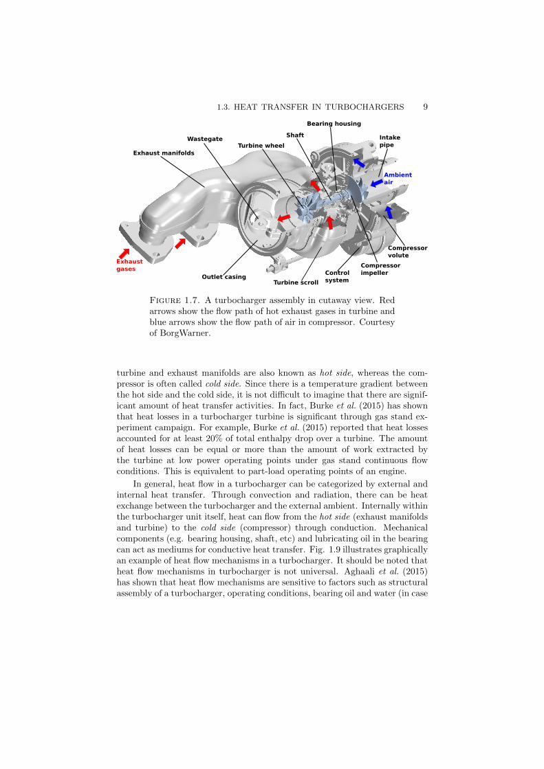
As discussed above, turbocharging is one of the methods of superchargingin ICE. The device that performs supercharging by means of turbocharging iscalled turbocharger. Fig. 1.7 shows the cutaway view of an automotive tur-bocharger assembly. A turbocharger consists of a radial turbine wheel and aradial compressor impeller connected on a common shaft. Hot exhaust gasesfrom the cylinder enter exhaust manifolds, directed and distributed circum-ferentially into the turbine wheel by a spiral shaped pipe called scroll. Thehot exhaust gases are ultimately being discharged into an outlet casing afterexpansion in the rotating wheel. As for the compressor side, ambient air issucked into the compressor impeller via an intake pipe and the compressed airflows around a volute before being guided into the engine cylinders for com-bustion. A high speed rotating shaft together with its bearing are enclosed ina bearing housing. Lubricating oil is filled in the small clearance between theshaft and the bearing to reduce mechanical friction and to enhance the lifespan

8 1. INTRODUCTION
270
300
280
400 400
270
260
280300
400
80
100
60
40
20
020 30 40 50 60 70 80 90 100
bsfc [g/kW-h]
contour lines
Turbocharged engine
Naturally aspirated engine
Mean piston speed
Maximum mean piston speedx 100 [%]
E
ng
ine t
orq
ue
Maxim
um
en
gin
e t
orq
ue
x 1
00 [
%]
Figure 1.6. Comparisons of brake specific fuel consumptionbsfc contour lines between turbocharged and naturally aspi-rated versions of the same spark-ignition SI engine on engineperformance map. The data at the vertical and horizontal axesare scaled to the maximum torque and maximum mean enginepiston speed, respectively. Adapted from Heywood (1988).
of turbocharger. A wastegate is coupled with a control system to bypass someamount of exhaust gases into the outlet casing without going through the tur-bine wheel. The control system is normally activated at high engine speed tolimit the shaft power. It should be noted that there exists other turbochargerassembly configurations (e.g. twin scroll, variable turbine, water-cooled, etc.)and readers can refer to turbocharging literature such as Baines (2005) for moreinformation.
1.3. Heat transfer in turbochargers
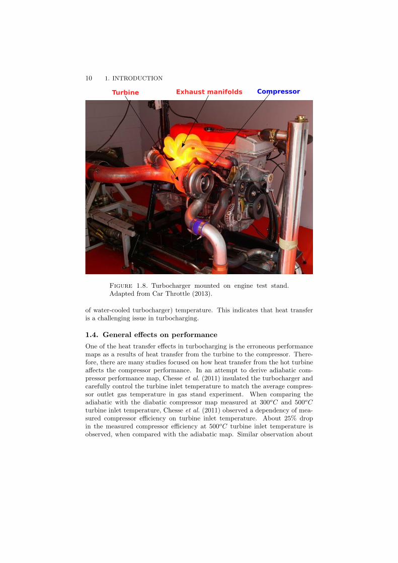
Fig. 1.8 shows a turbocharger operating under engine-like condition. Exhaustgases temperature can be above 900oC. As a result, the metallic walls of theexhaust manifolds and turbine are red glowing. On the other hand, relativelycold air is flowing in compressor and its downstream pipes. The red glowing
1.3. HEAT TRANSFER IN TURBOCHARGERS 9
Exhaust manifolds
Shaft Wastegate
Turbine wheel
Compressor
impeller
Bearing housing
Outlet casingTurbine scroll
Compressor
volute
Intake
pipe
Control
system
Exhaust
gases
Ambient
air
Figure 1.7. A turbocharger assembly in cutaway view. Redarrows show the flow path of hot exhaust gases in turbine andblue arrows show the flow path of air in compressor. Courtesyof BorgWarner.
turbine and exhaust manifolds are also known as hot side, whereas the com-pressor is often called cold side. Since there is a temperature gradient betweenthe hot side and the cold side, it is not difficult to imagine that there are signif-icant amount of heat transfer activities. In fact, Burke et al. (2015) has shownthat heat losses in a turbocharger turbine is significant through gas stand ex-periment campaign. For example, Burke et al. (2015) reported that heat lossesaccounted for at least 20% of total enthalpy drop over a turbine. The amountof heat losses can be equal or more than the amount of work extracted bythe turbine at low power operating points under gas stand continuous flowconditions. This is equivalent to part-load operating points of an engine.
In general, heat flow in a turbocharger can be categorized by external andinternal heat transfer. Through convection and radiation, there can be heatexchange between the turbocharger and the external ambient. Internally withinthe turbocharger unit itself, heat can flow from the hot side (exhaust manifoldsand turbine) to the cold side (compressor) through conduction. Mechanicalcomponents (e.g. bearing housing, shaft, etc) and lubricating oil in the bearingcan act as mediums for conductive heat transfer. Fig. 1.9 illustrates graphicallyan example of heat flow mechanisms in a turbocharger. It should be noted thatheat flow mechanisms in turbocharger is not universal. Aghaali et al. (2015)has shown that heat flow mechanisms are sensitive to factors such as structuralassembly of a turbocharger, operating conditions, bearing oil and water (in case
10 1. INTRODUCTION
Turbine CompressorExhaust manifolds
Figure 1.8. Turbocharger mounted on engine test stand.Adapted from Car Throttle (2013).
of water-cooled turbocharger) temperature. This indicates that heat transferis a challenging issue in turbocharging.
1.4. General effects on performance
One of the heat transfer effects in turbocharging is the erroneous performancemaps as a results of heat transfer from the turbine to the compressor. There-fore, there are many studies focused on how heat transfer from the hot turbineaffects the compressor performance. In an attempt to derive adiabatic com-pressor performance map, Chesse et al. (2011) insulated the turbocharger andcarefully control the turbine inlet temperature to match the average compres-sor outlet gas temperature in gas stand experiment. When comparing theadiabatic with the diabatic compressor map measured at 300oC and 500oCturbine inlet temperature, Chesse et al. (2011) observed a dependency of mea-sured compressor efficiency on turbine inlet temperature. About 25% dropin the measured compressor efficiency at 500oC turbine inlet temperature isobserved, when compared with the adiabatic map. Similar observation about

1.4. GENERAL EFFECTS ON PERFORMANCE 11
Legend:
Q= Heat transfer
C= Compressor
T= Turbine
BH= Bearing housing
S= Shaft
oil= Bearing oil
conv= convection
rad= radiation
QT,conv
QT,rad
QT->BH
QT->SQBH,conv
QBH,rad
QC,conv
QC,rad
QS->oil
Qoil->BH
Qc->air
QS->airExhaust
gases
Inlet
air
Figure 1.9. Simplified heat transfer mechanisms in tur-bocharger. Adapted from Romagnoli & Martinez-Botas(2012a).
strong dependency of compressor measured efficiency on heat transfer levelfrom the turbine to the compressor is also observed by several researchers likeCormerais et al. (2006), Rautenberg et al. (1984), and etc.
As for the turbine, most of the studies focus on reducing the errors inturbine outlet temperature prediction (e.g. Burke et al. 2015), and very littleattention is paid on how heat transfer affects the turbine performance. Al-though there are some studies about how heat transfer affects the performanceof turbine, literatures show contradicting conclusions about the effects of heattransfer on turbine performance. For example, Shaaban & Seume (2012) con-ducted an experimental study on a turbocharger operating under continuousflow conditions on a gas stand. The turbine is fed with cold and hot gases, whichrepresents adiabatic and diabatic conditions, respectively. The study showed
12 1. INTRODUCTION
that under hot gas conditions, turbine efficiency is about 20% (or equivalentto 55% in turbine power) lower as compared with cold gas conditions at lowspeed operating points. Furthermore, Shaaban & Seume (2012) found that theefficiency of insulated turbine operating under hot gas conditions is almost thesame as turbine operating with cold gas , and thus concluded that heat loss cansignificantly reduce the turbine power. The findings are in agreement with thetheoretical predictions about negative effects of heat transfer on turbochargerturbine performance (see Sec. 2.1.1).
On the other hand, Serrano et al. (2007) showed that turbine efficiency isabout 4% higher under hot gas conditions, as compared with cold gas condi-tions. The percentage of efficiency improvement is within measurement uncer-tainty range and the authors attributed this to the improvement of mechanicalefficiency due to lower lubricant oil viscosity in hot gas conditions. In an-other work, Sirakov & Casey (2013) studied how different heat transfer levelaffects the performance of turbocharger experimentally on gas stand steadyflow conditions. Heat transfer amount in turbocharger was varied by 1) cool-ing the center housing between the turbine and the compressor with water and2) changing the turbine inlet temperature. Their measurements showed thatpressure ratio is insensitive to the amount of heat transfer. The authors thenconcluded that heat transfer hardly affecting the aerothermodynamics of tur-bocharger. On the other hand, the apparent efficiency of the compressor andturbine is highly sensitive to heat transfer level, particularly at low speed andmass flow operating conditions. Sirakov & Casey (2013) attributed this to themisinterpretation of temperature rise in compressor due to heat transfer as ad-ditional work required to compress the air. Since turbine power and efficiencyare derived from compressor power and efficiency through power balance as-sumption (see Sec. 2.3), the turbine appears to have better efficiency than thereal condition. There is a shift of efficiency from the compressor to the turbineand the effects of heat transfer in turbocharger is simply wrong book-keepingof energy flow. In a numerical study by using Large Eddy Simulations (LES)with near wall treatment, Hellstrom & Fuchs (2010) found that difference inturbine shaft power is less than 1% between adiabatic and diabatic scenariosunder engine-like pulsating conditions.
1.5. Research scopes and objectives
It will be clear in Chap. 2 that turbocharging heat transfer is a very wideresearch field. In this thesis, the scope of study is focused on the understandingof the performance and flow physics in a turbocharger turbine, considering theheat transfer scenario. More specifically, the study focuses on the heat transferproblem in the exhaust manifolds and the turbine (the hot side), and neglectthe heat transfer effects on the compressor side. The system boundary in thestudy is limited to the fluid domain of exhaust manifolds and turbine.

1.5. RESEARCH SCOPES AND OBJECTIVES 13
Within the scope mentioned above, there is no consensus among researchersabout the effects of heat transfer on the performance of turbocharger turbine,as discussed in Sec. 1.4. Research gaps into connection to the effects of heattransfer on turbocharger turbine could be summarized as below.
1. Most of the literature are observation studies, i.e. direct comparisonsof turbine performance between adiabatic and diabatic (non-adiabatic)scenarios only. The mechanisms on how heat transfer affects the aerother-modynamics in the turbine is unknown.
2. Aerothermodynamics losses associated with heat transfer in turbine arenot identified and quantified to assist the understanding of how heattransfer affects the turbine performance.
3. There are limited studies in understanding the flow physics of tur-bocharger turbine operating under engine-like pulsating conditions withheat transfer. Upstream exhaust manifolds and flow instabilities effectson heat transfer and turbine performance are not understood.
Therefore, the overall goal of the study is to improve the understanding ofheat transfer and heat related losses of a turbocharger turbine operating underboth gas stand continuous flow and engine-like pulsating conditions. The long-term study aims to answer the following research questions for a turbochargerturbine.
1. How sensitive are the pressure ratio and turbine torque to various heattransfer level?
2. How aerothermodynamics in turbocharger turbine change with differentheat transfer levels, and how does this affect the turbine performance?
3. How much is the entropy generation (exergy destroyed) associated withheat transfer in each component of a turbocharger turbine?
4. How the upstream exhaust manifolds and flow instabilities affect heattransfer and turbine performance?
5. How different exhaust valve strategies affect the heat transfer and tur-bine performance?
Although one-dimensional model can provide fast results (see Sec. 2.2.2),it depends heavily on calibration with experimental data and does not provideinformation about the flow physics. Information about flow physics obtainedusing experiments can also be limited by several factors, such as difficulty intemperature measurement under highly pulsating engine-like conditions, flowfield visualization limitations due to constraint space and complex geometry.

14 1. INTRODUCTION
One the other hand, high-fidelity three dimensional transient ComputationalFluid Dynamics (CFD) enables one to capture flow driven instabilities in com-plex geometries and access to unsteady flow field data everywhere in the do-main. Detached Eddy Simulation (DES) is performed in this study to answerthe research questions formulated above and to achieve the thesis objective.

CHAPTER 2
Turbine and turbine performance metrics
This chapter first reviews the implications of heat transfer in turbochargingand current state-of-the-arts in turbocharging heat transfer research. Then,the chapter discusses the metrics used to evaluate the performance of a tur-bocharger turbine. Methods to evaluate the performance metrics in this studyare also stated in this chapter.
2.1. Heat transfer implications on turbocharging
Heat transfer is unavoidable in turbocharging due to the existence of temper-ature gradients, as discussed in Sec. 1.3. The implications of heat transfer onturbocharging are discussed in this section.
2.1.1. Performance deterioration
From both aerodynamics and thermodynamics point of views, there is no doubtthat heat transfer has negative effects on the performance of a turbocharger.Possible aerodynamics effects when there is heat transfer in turbomachinesmight be due to the change of velocity triangles associated with the changeof thermodynamic properties (density, absolute pressure and temperature offluid). For instance, taking turbine as an example, the turbine power is pro-portional to the rate of change of the angular momentum at the inlet andoutlet of the turbine wheel, as given by Eq. 2.1. It is also known as Eulerturbomachine equation.
WT = mT · ω · (r7,T · Cθ7,T − r8,T · Cθ8,T ) , (2.1)
where W is the power, m is the mass flow rate, ω is the rotational speed of theturbine wheel, r is the radius of the turbine wheel and Cθ is the tangential ve-locity component. Subscript 7 and 8 refer to the inlet and outlet of the turbinewheel, respectively. Subscript T means that the quantity is refering to turbine.
The turbine power WT in Eq. 2.1 can be related to the thermodynamicproperties by using ideal gas law and velocity triangle relationships as in Eq.2.2.
15

16 2. TURBINE AND TURBINE PERFORMANCE METRICS
WT =mT · ω · r7,T · tan(βT ) ·R
A7,T
T7,TP7,T
·[1− r8,T · tan(β8,T ) ·A7,T
r7,T · tan(β7,T ) ·A8,T
P7,T
P8,T
1
T7,T /T8,T
],
(2.2)
where P is the absolute pressure, T is the temperature, β is the absolute flowangle, A is the flow sectional area and R is the specific gas constant.
Absolute flow angle β and flow sectional area A are geometrical param-eters, and they are fixed for a chosen turbine. Then, from Eq. 2.2, it canbe seen that heat losses from turbine can alter the absolute pressure P andthe temperature T , and hence reduce the turbine power WT . It should beclarified that discussions above based on Eq. 2.1 and Eq. 2.2 have excludedaerothermodynamic losses for simplicity. There is a possibility of increasingaerothermodynamic losses associated with heat transfer.
In order to explore the thermodynamics effect on the performance of tur-bocharger, consider a simplified case, i.e. isentropic expansion of gas in theturbine wheel between a given constant pressure different. The change of gasenthalpy dh when gas is expanded between known pressure dP is given by
dh =dP
ρ=dP
P·R · T . (2.3)
As can be seen from Eq. 2.3, less work can be extracted if the working fluidapproaching the turbine wheel at lower temperature T as a result of priori heatlosses. The reverse applies to the compressor, i.e. more work is needed tocompress the air if heat transfer increses the working fluid temperature.
2.1.2. Erroneous performance maps derived from hot gas stand
It will be clear in Sec. 2.3.2 that the turbine power WT is not directly measuredin common industry practice. It is estimated from the compressor power WC ,which is related to the measured temperature difference across the compressor.Note that the compressor power WC derived from Eq. 2.9 in Sec. 2.3.1 is onlyvalid for adiabatic flow. Additional temperature rise in compressor due to heattransfer will be misintepreted as additional work required to compress the air.The situation is worsen by the fact that temperature measurements in hot gasstand are done at locations which do not coincide with the compressor stageboundary (see Sec. 2.3). These errors lead to miscalculation of compressorperformance, and thus affecting the estimation of turbine performance.
2.2. MODELING OF HEAT TRANSFER 17
2.1.3. Uncertainty in turbomachinery design and development
Turbomachinery is often developed from a baseline model by using conventionaltools such as one-dimensional code and Computational Fluid Dynamics (CFD).The developed turbomachinery is then tested on hot gas stand for performanceverification. Also, in the design and development process, aerothermodynam-ics losses are often correlated with experimental data. Erroneous performancemaps due to heat transfer can cause serious uncertainty when one try to un-derstand the performance and aerothermodynamics loss mechanisms.
2.1.4. Sub-optimal turbocharged engine system performance
The performance maps derived from the hot gas stand is used by engine manu-facturers in engine powertrain simulations to select the optimum turbochargerfor an engine. Engine powertrain simulation is typically done in an iterativeway. It requires the inputs of several compressor and turbine performance mapsand these performance maps are normally provided by different turbochargermanufactures. Unfortunately, heat transfer conditions on hot gas stands of dif-ferent turbocharger manufacturers might be different and it is an unknown toengine manufacturers. If there are errors in the performance maps associatedwith heat transfer, engine manufacturers might face the risks of developing asub-optimal turbocharged engine system. Also, assuming that there is no heattransfer related errors in the performance maps, different heat transfer levelbetween the hot gas stand and real engine conditions can also cause inaccuracyin the prediction of engine system performance.
2.1.5. Thermal failure
Due to the pulsating nature of the exhaust flow and high heat transfer rate, themetalic components in the turbocharger are subjected to rapid thermal cycles.This induces thermal stress and a turbocharger is highly exposed to the risk ofmechanical failures such as thermal fatigue.
2.2. Modeling of heat transfer
Turbochrging heat transfer is a very wide research field. This section reviewsand summarizes the research focus related to turbocharging heat transfer, inparticular the heat transfer modeling in turbocharging.
2.2.1. Quantification of heat transfer
In general, quantification of the amount of heat transfer is the first step inturbocharging heat transfer research. The amount of heat transfer at variouscomponents is normally estimated by measuring the temperature at various lo-cations (e.g. turbine scroll/compressor volute inner and outer walls, inlet andoutlet of lubricant oil, etc.) in experiment. For example, Baines et al. (2010)

18 2. TURBINE AND TURBINE PERFORMANCE METRICS
estimated that the fraction of total turbine heat transfer losses to the exter-nal environment, the lubricating oil and the compressor is 70% , 25% and 5%respectively in gas stand experiment. Another good example of heat transferquantification work is the on-engine experimental measurement on a water-cooled turbocharger by Aghaali et al. (2015). Aghaali et al. (2015) reportedthat external heat transfer of the compressor and bearing housing is less signif-icant, when compared with the internal heat transfer from the turbine to thebearing housing and from the bearing housing to the compressor. Furthermore,the authors also showed that the amount of heat transfer in various componentsis sensitive to external factors such as the ambient air ventilation. It should benoted that the outcomes of these experimental quantification studies are nor-mally used as inputs to one-dimensional models for performance corrections.
2.2.2. One-dimensional modelling
In general, industry relies on iterative engine simulation to match the tur-bocharger and the engine performance. Each iteration of engine simulation in-volves calculations of performances over many engine operating points. There-fore, one of the turbocharging heat transfer research focus is to develop lowcomputational cost simplified one-dimensional heat transfer models to correctthe heat transfer effects and to improve the accuracy of performance predic-tion. There are different approaches adopted by researchers in one-dimensionalheat transfer modelling. A few common approaches are summarized below asexamples.
1. The most basic method is the application of correction factors thatcorrelate the results of one-dimensional engine simulation to the exper-imental results. For example, Aghaali & Angstrom (2012) introducedefficiency and mass flow multipliers to the gas stand measured compres-sor and turbine performance maps to correct the heat transfer effects inone-dimensional gas dynamics engine simulation code. Similarly, Junget al. (2002) suggested to separate the gas stand measured turbine ef-ficiency into aerodynamics and heat transfer contributions, and thencorrelate the heat transfer part based on the theory of heat exchangerwith flow dependent effectiveness.
2. In reality, heat transfer and work transfer occur simultaneously in turbo-machinery. For simplicity reason, it is also common to assume that heattransfer and work transfer in turbine and compressor occurs separately,i.e. independent from each other. In this approach, the gas expan-sion/compression in rotating component is treated as adiabatic. It is as-sumed that heat transfer in the rotating components is likely to be smallas compared with components like turbine scroll and compressor volute.As with the modelling of heat transfer, there are two different method-ologies adopted by researchers. Researchers like Cormerais et al. (2009)
2.2. MODELING OF HEAT TRANSFER 19
and Serrano et al. (2010) assume that heat transfer occurs at constantpressure after gas expansion/compression in the rotating component,while Romagnoli & Martinez-Botas (2012b) and Burke et al. (2015) pre-fer to lump all heat transfer before/after the gas expansion/compressionprocess. Regardless of the methodologies, temperature measurementsare done at various locations (e.g. turbine scroll/compressor volute in-ner and outer walls, inlet and outlet of lubricant oil, etc.) in gas standor on-engine experiment. Energy balance is then applied to estimatethe amount of heat transfer.
3. One-dimensional heat transfer models are heavily dependent on heattransfer correlations. Conventional heat transfer correlations are for-mulated based on experiment measurements of simple flow situations(e.g. pipe flow, flow around cylinder, and etc.), which might not besuitable for turbocharging applications. Therefore, there are effortsin establishing new heat transfer correlations based on gas stand/on-engine experimental results or theory. For example, Baines et al. (2010)performed temperature measurements on three different turbochargersmounted on gas stand. By using experimental measurement results,Baines et al. (2010) developed correlation among Nusselt number Nu,Reynolds number Re and Prandtl number Pr. Another example canbe seen in the work by Romagnoli & Martinez-Botas (2012b), in whichsimilar correlation is derived based on straight pipe theory.
It should be noted that although one-dimensional heat transfer modelscan provide fast results, they depend heavily on experimental correlations.Careful calibration of one-dimensional model with experimental data has tobe done before it can be used to predict performance. The correlations es-tablished for a particular turbocharger on a particular engine are most likelyinvalid for another turbocharger or engine (Jung et al. 2002). Furthermore, one-dimensional models cannot provide information such as flow fields. Therefore,one-dimensional models are not suitable to study loss mechanisms associatedwith heat transfer.
2.2.3. Three dimensional modelling
The most sophisticated three-dimensional modelling approach is conjugate heattransfer (CHT), which involves solving the fluid flow field and solid body heattransfer in a coupling way. This approach is computational expensive mainlybecause of slow convergence rate due to large time scale disparity in the fluidand solid domain. He & Oldfield (2011) estimated that the ratio of conductivetime scale in the solid domain to the convective time scale in the fluid domainis about 10,000. Therefore, there are only limited CHT study in turbochargingheat transfer research. One of the prominent CHT studies in turbocharger isthe steady state CHT simulation by Bohn et al. (2005). Boundary conditions
20 2. TURBINE AND TURBINE PERFORMANCE METRICS
for the fluid domain are the conventional experiment measured data, whereasexternal surface temperature obtained from thermographic camera during theexperiment is imposed on the solid domain as boundary condition. The studymainly focused on analysing the heat transfer path from the hot turbine to thecompressor. One of the important findings is that heat transfer in compressoroccurs mainly after the rotating impeller. This observation formed the basicassumption of one-dimensional heat transfer modelling, i.e. heat transfer takesplace after work transfer in compressor. There are also a few other CHTstudies involving heat transfer in turbocharger, but most of the studies focusedon predicting the solid wall temperature or heat transfer coefficient for thermalstructural analysis purpose (see e.g. Yamagata 2006).
A relatively lower cost three-dimensional modelling approach is Computa-tional Fluid Dynamics (CFD), which involves the fluid domain only. There aremany CFD studies focusing on performance prediction, optimization and flowfield analysis under both gas stand continuous flow conditions and engine-likepulsating conditions, but most of the studies were performed under adiabaticassumption (see e.g. Galindo et al. 2013). LES simulation on a turbochargerturbine under engine-like pulsating condition performed by Hellstrom & Fuchs(2010) represents one of the very few published literature that consider theeffects of heat transfer. In Hellstrom & Fuchs (2010) study, heat transfer ismodelled by imposing constant wall temperature on the turbine scroll and out-let diffuser, but the rotating turbine wheel is treated as adiabatic. It should benoted that exhaust manifolds are not included in Hellstrom & Fuchs (2010)’sthree-dmensional model. Therefore, the upstream exhaust manifolds and flowinstabilities effects on heat transfer and turbine performance remain unclear.Also, since only a single operating condition is studied by Hellstrom & Fuchs(2010), how different exhaust valve strategies are affecting the heat transferand turbine performance is also unknown.
There are also efforts in coupling CFD or one-dimensional flow solvers withFinite Element Analysis (FEA) solver for industry iterative design and opti-mization purpose. In this approach, wall heat transfer coefficient is computedby flow solver and the results are mapped onto the fluid-solid wall for FEAcomputations. This approach is mainly used for sructural thermal analysis,e.g. prediction of metal wall temperature (see e.g. Karamavruc 2016).
2.3. Turbocharger performance and assessment
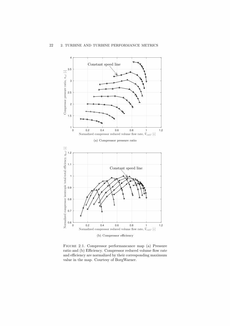
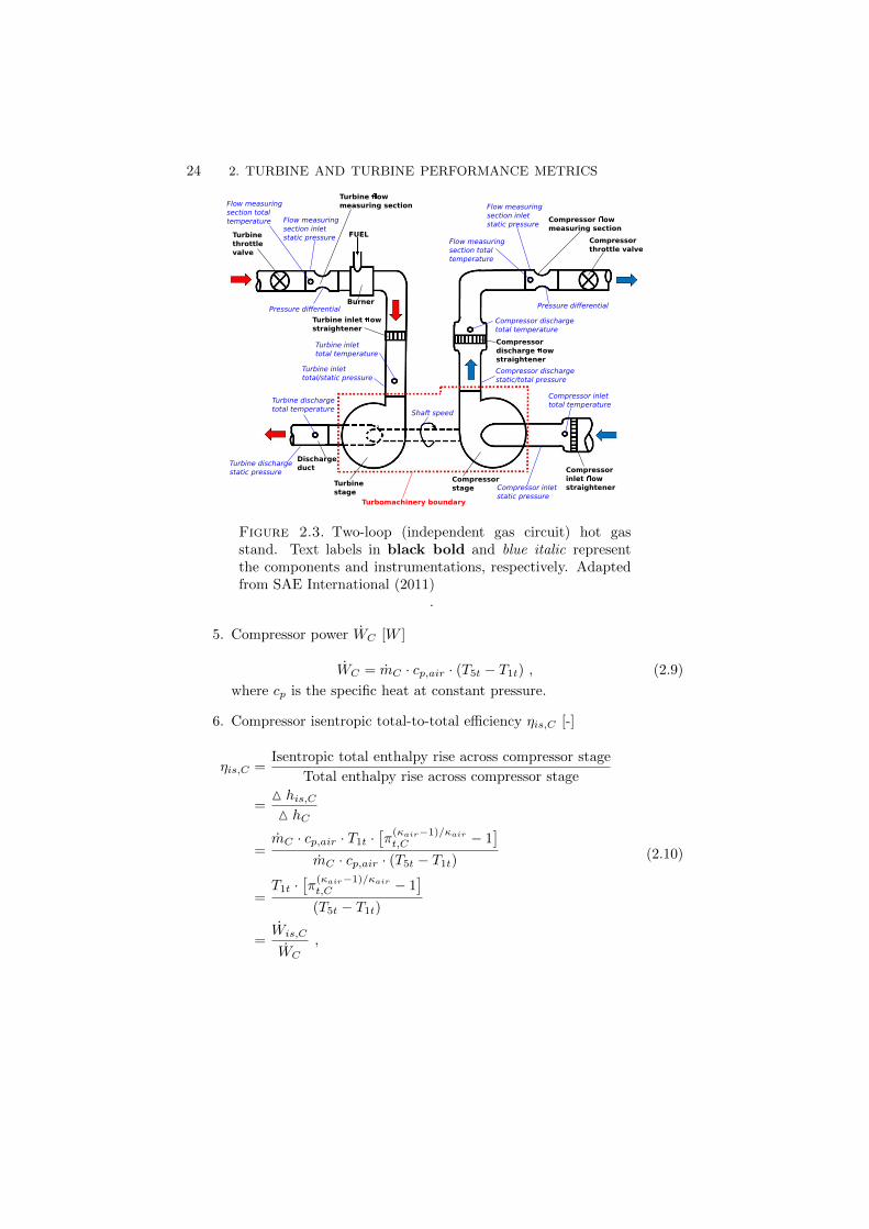
The performance of a turbocharger can be described by a separate compressorperformance map and its corresponding turbine performance map. Examplesof the compressor and turbine performance maps are depicted in Fig. 2.1 and2.2, respectively. These performance maps are derived from measurements ofmass flow rate, pressure ratio, shaft speed and isentropic efficiencies under hotgas stand continuous flow conditions. The most commonly used hot gas standis the two-loop circuit, as depictd schematically in Fig. 2.3. The locations of

2.3. TURBOCHARGER PERFORMANCE AND ASSESSMENT 21
instrumentations are also indicated in Fig. 2.3. Note that measurements aredone at locations which do not coincide with the turbomachinery boundary,i.e. at locations further upstream and downstream of the compressor and theturbine.
2.3.1. Compressor performance characteristics
The compressor of a turbocharger is normally characterized by the followingparameters. Subscript t denotes total quantity and subscript C means that thequantity refers to the compressor. Furthermore, subscripts 1 and 5 refers tothe inlet and outlet measurement locations on the compressor side, respectively(see Fig. 2.3).
1. Compressor pressure ratio πt,C [-]
πt,C =Outlet air total absolute pressure [kPa]
Inlet air total absolute pressure [kPa]
=P5t
P1t.
(2.4)
2. Compressor air mass flow mC [kg/s]
mC = kg/s of air mass flow through the compressor (2.5)
3. Compressor reduced volume flow rate Vred,C [m3/s]
Vred,C =V1,C√T1t
T1t,ref
, (2.6)
where
V1,C =mC
P1t
Rair·T1t
. (2.7)
4. Compressor reduced rotational speed nred,C [rpm]
nred,C =ω√
T1t/T1t,ref, (2.8)
where ω is the shaft speed, which is the same for both compressor andturbine. ref in the subscript is the abbreviation for reference.
22 2. TURBINE AND TURBINE PERFORMANCE METRICS
0 0.2 0.4 0.6 0.8 1 1.2
Normalized compressor reduced volume flow rate, Vred,C [-]
1
1.5
2
2.5
3
3.5
4
Com
pressor
pressure
ratio,
πt,C[-]
Constant speed line
(a) Compressor pressure ratio
0 0.2 0.4 0.6 0.8 1 1.2
Normalized compressor reduced volume flow rate, Vred,C [-]
0.6
0.7
0.8
0.9
1
1.1
1.2
Normalized
compressor
isentrop
ictotal-totaleffi
ciency,ηis,C
[-]
Constant speed line
(b) Compressor efficiency
Figure 2.1. Compressor performancance map (a) Pressureratio and (b) Efficiency. Compressor reduced volume flow rateand efficiency are normalized by their corresponding maximumvalue in the map. Courtesy of BorgWarner.

2.3. TURBOCHARGER PERFORMANCE AND ASSESSMENT 23
1 1.5 2 2.5 3 3.5 4
Turbine pressure ratio, π6t8s,T [-]
0.6
0.7
0.8
0.9
1
1.1
1.2
Normalized
turbineflow
param
eter,TFP[-]
P
Constant speed line
(a) Turbine flow parameter
1 1.5 2 2.5 3 3.5 4
Turbine pressure ratio, π6t8s,T [-]
0.6
0.7
0.8
0.9
1
1.1
1.2
Normalized
combined
turbinexmechan
ical
efficiency,ηis,Txηm[-]
PConstant speed line
(b) Turbine efficiency
Figure 2.2. Turbine performancance map (a) Pressure ratioand (b) Efficiency. Turbine flow parameter and efficiency arenormalized by their corresponding maximum value in the map.P is the operating point for simulation under continuous flowcondition. Courtesy of BorgWarner.
24 2. TURBINE AND TURBINE PERFORMANCE METRICS
Turbine
stage
Compressor
stage
Compressor
inlet ow
straightener
Turbine inlet ow
straightener
Compressor
discharge ow
straightener
Turbine ow
measuring section
Turbine
throttle
valve
Burner
Compressor
throttle valve
FUEL
Discharge
duct
Compressor ow
measuring section
Compressor inlet
total temperature
Compressor inlet
static pressure
Compressor discharge
static/total pressure
Compressor discharge
total temperature
Flow measuring
section total
temperature
Shaft speed
Turbine inlet
total temperature
Turbine inlet
total/static pressure
Turbine discharge
total temperature
Turbine discharge
static pressure
Pressure differential
Flow measuring
section inlet
static pressure
Flow measuring
section total
temperature Flow measuring
section inlet
static pressure
Pressure differential
Turbomachinery boundary
Figure 2.3. Two-loop (independent gas circuit) hot gasstand. Text labels in black bold and blue italic representthe components and instrumentations, respectively. Adaptedfrom SAE International (2011)
.
5. Compressor power WC [W ]
WC = mC · cp,air · (T5t − T1t) , (2.9)
where cp is the specific heat at constant pressure.
6. Compressor isentropic total-to-total efficiency ηis,C [-]
ηis,C =Isentropic total enthalpy rise across compressor stage
Total enthalpy rise across compressor stage
=M his,CM hC
=mC · cp,air · T1t ·
[π(κair−1)/κairt,C − 1
]mC · cp,air · (T5t − T1t)
=T1t ·
[π(κair−1)/κairt,C − 1
](T5t − T1t)
=Wis,C
WC
,
(2.10)
2.3. TURBOCHARGER PERFORMANCE AND ASSESSMENT 25
where κ is the specific heat ratio. Note that the compressor work WC depictedin Eq. 2.9 is derived from the measured total temperature difference at lo-cations further upstream and downstream of the compressor, as illustrated inFig. 2.3.
2.3.2. Turbine performance characteristics
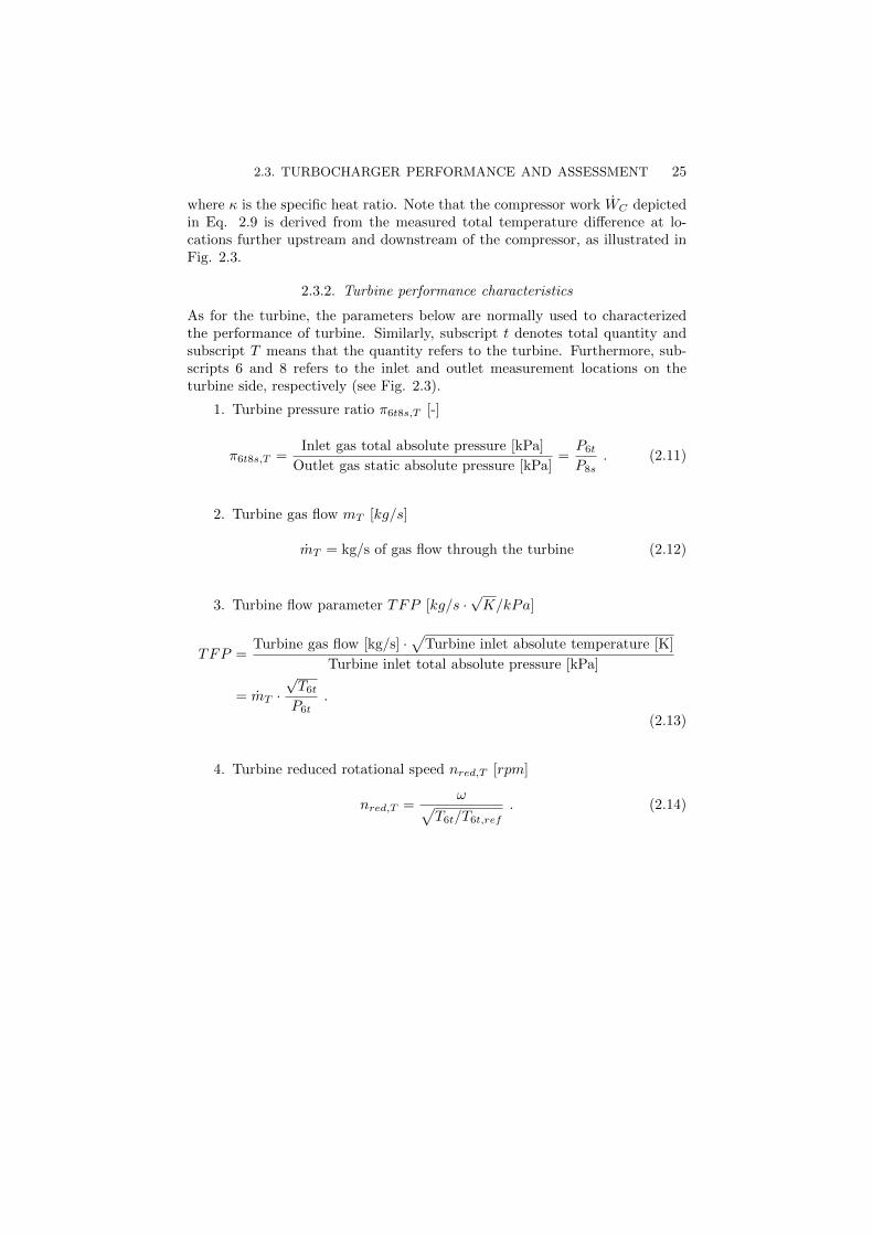
As for the turbine, the parameters below are normally used to characterizedthe performance of turbine. Similarly, subscript t denotes total quantity andsubscript T means that the quantity refers to the turbine. Furthermore, sub-scripts 6 and 8 refers to the inlet and outlet measurement locations on theturbine side, respectively (see Fig. 2.3).
1. Turbine pressure ratio π6t8s,T [-]
π6t8s,T =Inlet gas total absolute pressure [kPa]
Outlet gas static absolute pressure [kPa]=P6t
P8s. (2.11)
2. Turbine gas flow mT [kg/s]
mT = kg/s of gas flow through the turbine (2.12)
3. Turbine flow parameter TFP [kg/s ·√K/kPa]
TFP =Turbine gas flow [kg/s] ·
√Turbine inlet absolute temperature [K]
Turbine inlet total absolute pressure [kPa]
= mT ·√T6tP6t
.
(2.13)
4. Turbine reduced rotational speed nred,T [rpm]
nred,T =ω√
T6t/T6t,ref. (2.14)

26 2. TURBINE AND TURBINE PERFORMANCE METRICS
5. Mechanical efficiency ηm [-]
ηm =WC
WT
=WC
WC + Wf
.
(2.15)
6. Combined turbine × mechanical efficiency ηis,T × ηm [-]
ηis,T × ηm =Total enthalpy rise across compressor stage
Isenropic total enthalpy drop across turbine stage
=M hCM his,T
=mC · cp,air · (T5t − T1t)
mT · cp,exh · T6t ·[1− π−(κexh−1)/κexh6t8s,T
]=
WC
Wis,T
,
(2.16)
where subscript exh is the abbreviation for exhaust gas. From Eq. 2.15, it canbe seen that the turbine power WT is related to the compressor work WC andfriction losses Wf (associated with the bearing systems) by considering powerbalance on the common shaft. Although some special gas stand facilities canmeasure turbine work directly by using dynamometer (Szymko et al. 2007),direct turbine torque measurement by using dynamometer is uncommon inindustrial gas stands.
2.4. Turbine power and torque
Since the scope of the study is limited to the turbine in this study, turbine powerWT cannot be estimated from the total enthalpy drop across the compressorstage, as depicted in the numerator of Eq. 2.16. Also, heat transfer is involvedand hence the total enthalpy drop across the turbine stage cannot represent thework extracted by the turbine wheel. Therefore, turbine power and torque in
this study are computed by integrating total forces ~ftotal (pressure and shear)over the rotating blade surfaces Srotate, as depicted in Eq. 2.17 and Eq. 2.18.
WT =
¨
Srotate
[(~r × ~ftotal) · ~ω] dS , (2.17)
~τ =
¨
Srotate
(~r × ~ftotal) dS , (2.18)
2.6. EXERGY ANALYSIS 27
where ~r is the position vector relative to the origin of the rotating referenceframe.
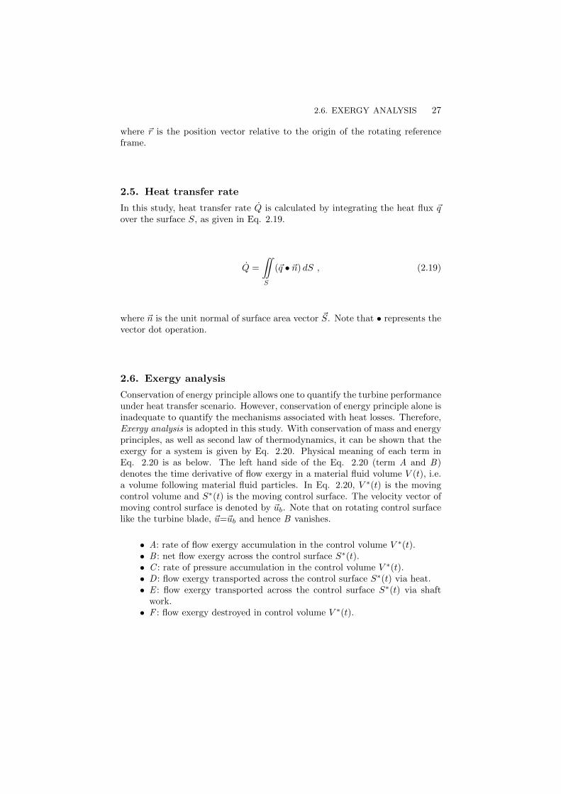
2.5. Heat transfer rate
In this study, heat transfer rate Q is calculated by integrating the heat flux ~qover the surface S, as given in Eq. 2.19.
Q =
¨
S
(~q • ~n) dS , (2.19)
where ~n is the unit normal of surface area vector ~S. Note that • represents thevector dot operation.
2.6. Exergy analysis
Conservation of energy principle allows one to quantify the turbine performanceunder heat transfer scenario. However, conservation of energy principle alone isinadequate to quantify the mechanisms associated with heat losses. Therefore,Exergy analysis is adopted in this study. With conservation of mass and energyprinciples, as well as second law of thermodynamics, it can be shown that theexergy for a system is given by Eq. 2.20. Physical meaning of each term inEq. 2.20 is as below. The left hand side of the Eq. 2.20 (term A and B)denotes the time derivative of flow exergy in a material fluid volume V (t), i.e.a volume following material fluid particles. In Eq. 2.20, V ∗(t) is the movingcontrol volume and S∗(t) is the moving control surface. The velocity vector ofmoving control surface is denoted by ~ub. Note that on rotating control surfacelike the turbine blade, ~u=~ub and hence B vanishes.
• A: rate of flow exergy accumulation in the control volume V ∗(t).• B : net flow exergy across the control surface S∗(t).• C : rate of pressure accumulation in the control volume V ∗(t).• D : flow exergy transported across the control surface S∗(t) via heat.• E : flow exergy transported across the control surface S∗(t) via shaft
work.• F : flow exergy destroyed in control volume V ∗(t).
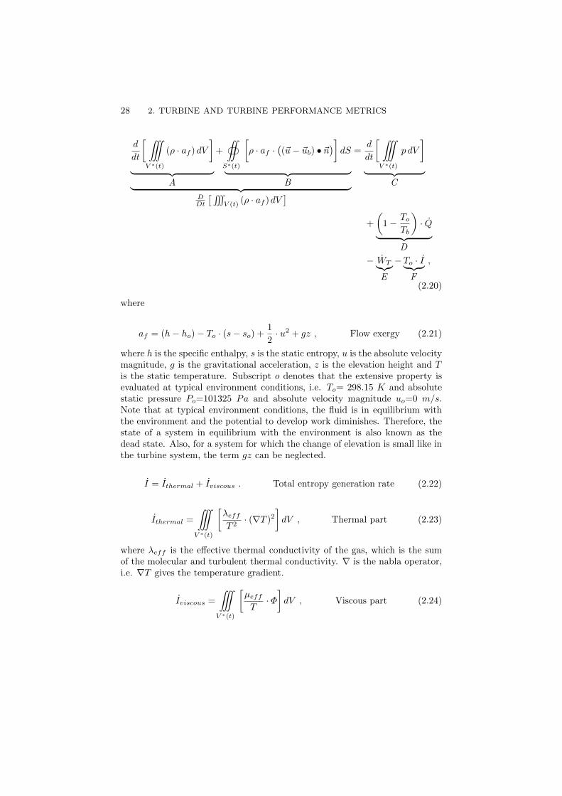
28 2. TURBINE AND TURBINE PERFORMANCE METRICS
d
dt
[˚V ∗(t)
(ρ · af ) dV
]︸ ︷︷ ︸
A
+
‹
S∗(t)
[ρ · af ·
((~u− ~ub) • ~n
)]dS
︸ ︷︷ ︸B︸ ︷︷ ︸
DDt
[˝V (t)
(ρ · af )dV]
=d
dt
[˚V ∗(t)
p dV
]︸ ︷︷ ︸
C
+
(1− To
Tb
)· Q︸ ︷︷ ︸
D
− WT︸︷︷︸E
−To · I︸ ︷︷ ︸F
,
(2.20)
where
af = (h− ho)− To · (s− so) +1
2· u2 + gz , Flow exergy (2.21)
where h is the specific enthalpy, s is the static entropy, u is the absolute velocitymagnitude, g is the gravitational acceleration, z is the elevation height and Tis the static temperature. Subscript o denotes that the extensive property isevaluated at typical environment conditions, i.e. To= 298.15 K and absolutestatic pressure Po=101325 Pa and absolute velocity magnitude uo=0 m/s.Note that at typical environment conditions, the fluid is in equilibrium withthe environment and the potential to develop work diminishes. Therefore, thestate of a system in equilibrium with the environment is also known as thedead state. Also, for a system for which the change of elevation is small like inthe turbine system, the term gz can be neglected.
I = Ithermal + Iviscous . Total entropy generation rate (2.22)
Ithermal =
˚
V ∗(t)
[λeffT 2· (∇T )2
]dV , Thermal part (2.23)
where λeff is the effective thermal conductivity of the gas, which is the sumof the molecular and turbulent thermal conductivity. ∇ is the nabla operator,i.e. ∇T gives the temperature gradient.
Iviscous =
˚
V ∗(t)
[µeffT· Φ]dV , Viscous part (2.24)

2.7. BEJAN NUMBER 29
where µeff is the effective dynamic viscosity of the gas, which is the sum ofthe molecular and turbulent dynamic viscosity. Φ is defined as
Φ = τij ·∂ui∂xj
Mechanical dissipation function
= 2 · Sij · Sij −2
3· Skk · Skk .
(2.25)
where
Sij =1
2·( ∂ui∂xj
+∂uj∂xi
). Strain rate tensor (2.26)
2.7. Bejan number
Bejan nuber Be is a non-dimensional parameter to indicate the relative im-portance of viscous irreversibility Iviscous and thermal irreversibility Iviscous(Bejan 1995). It is defined as in Eq. 2.27.
Be =1
1 + IviscousIthermal
, (2.27)
where Iviscous/Ithermal is also known as irreversibility factor. Note that Be = 0means that the irreversibility is purely due to viscous effect, whereas Be = 1indicates that the irreversibility is purely due to thermal effect.
CHAPTER 3
Turbine flow modeling
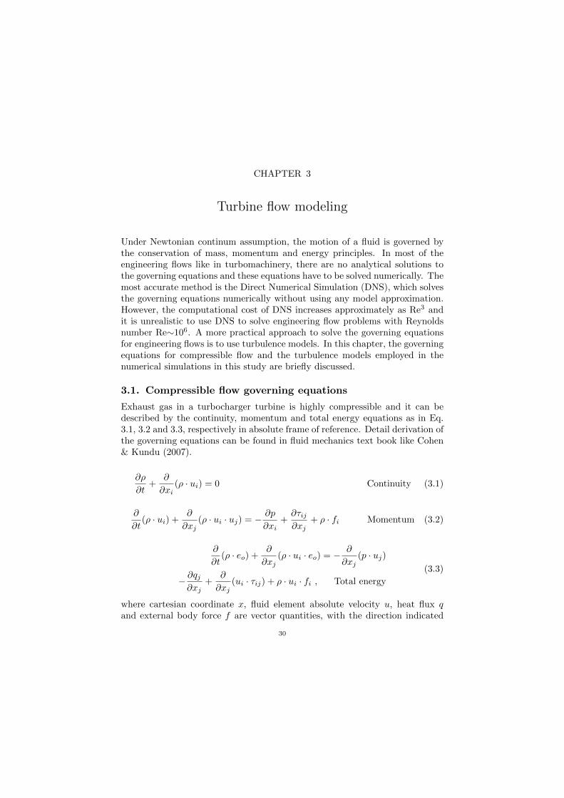
Under Newtonian continum assumption, the motion of a fluid is governed bythe conservation of mass, momentum and energy principles. In most of theengineering flows like in turbomachinery, there are no analytical solutions tothe governing equations and these equations have to be solved numerically. Themost accurate method is the Direct Numerical Simulation (DNS), which solvesthe governing equations numerically without using any model approximation.However, the computational cost of DNS increases approximately as Re3 andit is unrealistic to use DNS to solve engineering flow problems with Reynoldsnumber Re∼106. A more practical approach to solve the governing equationsfor engineering flows is to use turbulence models. In this chapter, the governingequations for compressible flow and the turbulence models employed in thenumerical simulations in this study are briefly discussed.
3.1. Compressible flow governing equations
Exhaust gas in a turbocharger turbine is highly compressible and it can bedescribed by the continuity, momentum and total energy equations as in Eq.3.1, 3.2 and 3.3, respectively in absolute frame of reference. Detail derivation ofthe governing equations can be found in fluid mechanics text book like Cohen& Kundu (2007).
∂ρ
∂t+
∂
∂xi(ρ · ui) = 0 Continuity (3.1)
∂
∂t(ρ · ui) +
∂
∂xj(ρ · ui · uj) = − ∂p
∂xi+∂τij∂xj
+ ρ · fi Momentum (3.2)
∂
∂t(ρ · eo) +
∂
∂xj(ρ · ui · eo) = − ∂
∂xj(p · uj)
− ∂qj∂xj
+∂
∂xj(ui · τij) + ρ · ui · fi , Total energy
(3.3)
where cartesian coordinate x, fluid element absolute velocity u, heat flux qand external body force f are vector quantities, with the direction indicated
30

3.1. COMPRESSIBLE FLOW GOVERNING EQUATIONS 31
by indices i,j and k. τij is the shear stress tensor. The scalar quantities aretime t, density ρ, absolute static pressure p and total energy per unit volumeeo = e + 1
2 · ui · ui . e is the specific internal energy and it can be related tospecific enthalpy h by Eq. 3.4. Flow variables here are the instanteneous value.
e = h− p
ρ. (3.4)
The specific enthalpy h can be further related to temperature by assumingthermally perfect gas as in Eq. 3.5.
h = cp · T , (3.5)
where cp is the specific heat capacity at constant pressure, which is a functionof polynomial temperature.
For Newtonian fluid, shear stress tensor τij can be related to the isotropicpart of the velocity gradient tensor, i.e. strain rate tensor Sij (see Eq. 2.26)via Eq. 3.6 with Stokes assumption.
τij = 2 · µ ·(Sij −
1
3· Skkδij
), (3.6)
where δij is the mathematical Kronecker delta function. µ is the temperaturedependence molecular dynamic viscosity of the fluid, which is modeled by usingSutherland’s law as according to Eq. 3.7.
µ = µref ·(Tref + S
T + S
)·( T
Tref
) 32 , (3.7)
where S=111 K is the Sutherland’s constant. µref=1.716x10⁻⁵ Pa− s is themolecular dynamic viscosity of the fluid at reference temperature Tref=273.15K.
As for the heat flux vector ~q, it is modeled by using Fourier’s law of con-duction as given in Eq. 3.8.
qj = λ · ∂T∂xj
, (3.8)
where λ is the molecular thermal conductivity of the fluid. Similar to µ, thedependence of λ on temperature is also modeled by using Sutherland’s law.The reference molecular thermal conductivity λref is 0.02614 W/m − K andthe Sutherland’s constant S is 194 K.
From the discussions hereinbefore, it can be seen that there are six un-knonws (pressure, temperature, density and three velocity components), butonly five equations are available. In order to close the system of equations,ideal gas law as given in Eq. 3.9 is used to couple the momentum equationsand the total energy equations.
32 3. TURBINE FLOW MODELING
p = ρ ·R · T , (3.9)
where R is the specific gas constant given by Eq. 3.10.
R =RM
, (3.10)
where R is the universal gas constant andM is the molecular weight of the gas.Since the temperature considered in this study is well below the temperatureof gas dissociation/association, molecular weight M of the gas is unchangedand therefore R is a constant for a specific gas.
3.2. Reynolds Averaged Navier-Stokes (RANS) modeling
The most common approach to study turbulence is to split the instanteneousflow variable φ into a mean part φ and a fluctuating part φ′, as according toReynolds decomposition in Eq. 3.11. The average as defined in Eq. 3.12 is alsotermed Reynolds averaging.
φ(x, y, z, t) = φ(x, y, z, t) + φ′(x, y, z, t) , (3.11)
where
φ(x, y, z, t) = limT→∞
1
T
ˆ t+T
t
φdt︸ ︷︷ ︸time averaging
or limN→∞
1
N
N∑n=1
φ︸ ︷︷ ︸ensemble averaging
(3.12)
φ′ ≡ 0 . (3.13)
In Reynolds Averaged Navier-Stokes (RANS) modeling approach, Reynoldsdecomposition is applied to the instanteneous flow variables in the governingequations and equation of state first, and then Reynolds averaging is performed.Note that density fluctuation ρ′ is assumed to be zero in RANS approach, i.e.ρ = ρ. This assumption is appropriate in most cases because turbulent fluctua-tions do not cause significant density fluctuations, except in highly compressibleflows and hypersonic flows. The resulting mean flow equations are given in Eq.3.14 to 3.17.
∂ρ
∂t+
∂
∂xj(ρ · uj) = 0 , (3.14)
∂
∂t(ρ · ui) +
∂
∂xj(ρ · ui · uj) = − ∂p
∂xi+
∂
∂xj(τ ij + τ turbij ) + ρ · f i , (3.15)

3.2. REYNOLDS AVERAGED NAVIER-STOKES (RANS) MODELING 33
∂
∂t
[ρ ·{
(e+1
2· ui · ui) +
1
2· u′i · u′i
}]+
∂
∂xj
[ρ · uj ·
{(h+
1
2· ui · ui) +
1
2· u′i · u′i
}]=
∂
∂xj
[ui · (τ ij + τ turbij )− qj − ρ · u′j · h′ + τij · u′i − ρ · u′j ·
1
2· u′i · u′i
]+ρ · ui · fi ,
(3.16)
p = ρ ·R · T , (3.17)
The mean flow equation Eq. 3.15 is usually known as Reynolds-averagedNavier-Stokes equation (RANS). τ ij in the equation is the mean viscous shearstress tensor and it is the time-average net momentum flux by molecular mo-tion. τ turbij is known as turbulent stress or Reynolds stress tensor, as definedin Eq. 3.18. It represents the time-average transport of momentum by macro-scopic velocity fluctuations.
τ turbij = −ρ · u′i · u′j . (3.18)
Eq. 3.16 is the Reynolds averaged total energy equation. 12 ·u
′i · u′i appears
on the left hand side of Eq. 3.16 is the kinetic energy due to turbulent fluctua-tions, k. qj is the molecular transport of heat, whereas turbulent transport of
heat qturbj (also known as turbulent heat flux) is represented by the correlationbetween u′j and h′. Molecular diffusion and turbulent transport of turbulent
kinetic energy is denoted by τij · u′i and ρ ·u′j · 12 · u′i · u′i, respectively. ρ ·ui · fi
represents the work done by the external body force. ui · (τ ij + τ turbij ) is thetotal work done by the viscous and turbulence shear stress.
Note that after the averaging process, there are more unknowns than thenumber of equations. This requires some approximations and turbulence mod-eling to close the system of equations. The most common approach to approx-imate the Reynolds stress term in the momentum equation (Eq. 3.15) is theeddy viscosity model, which is based on Boussinesq approximation as given inEq. 3.19. Similarly, the turbulent heat flux qturbj in the total energy equa-tion is also modeled by using Boussinesq approximation as according to Eq.3.20. As for the molecular diffusion and turbulent transport terms in Eq. 3.16,approximation as depicted in Eq. 3.21 is adopted.
− ρ · ui · uj ≈ 2 · ρ · νt · (Sij −2
3· Skk · δij)−
2
3· ρ · k · δij , (3.19)
34 3. TURBINE FLOW MODELING
qturbj = ρ · u′j · h′ ≈ −ρ · νt · cpPrt
∂T
∂xj, (3.20)
τij · u′i − ρ · u′j ·1
2· u′i · u′i ≈ ρ · (ν +
νtσk
) · ∂k∂xj
, (3.21)
where νt is the turbulent viscosity (or eddy viscosity), ν(= µρ ) is the molecular
kinematic viscosity, Sij is the mean strain rate tensor, Prt is the turbulentPrandtl number and σk is the Schmidt number.
Approximations discussed above alone are not sufficient to close the systemof equations and turbulence model is necessary. Many turbulence models havebeen developed over the years. Examples of popular turbulence models arethe one-equation Spalart-Allmaras model (Spalart et al. 1992), two-equationk− ε model (Launder & Spalding 1974) and k− ω model Wilcox et al. (1998),etc. However, the discussions hereinafter will focus on the two-equation ShearStress Transport (SST) k − ω model (Menter 1994) because it is the RANSmodel used in this study.
One of the limitations of k− ε model is that it cannot be integrated to thewall and hence it is invalid in the near-wall region. It has difficulty in capturingproper turbulent boundary layers behaviour up to separation (Wilcox 1993).Although k−ω model is shown to be more robust and accurate in the near-wallregion, it is strongly sensitive to the value of specific dissipation rate ω outsidethe boundary layer, i.e. in the freestream (Menter 1992). Here, SST k − ωmodel aims to combine the advantage of k − ω model in the near-wall regionwith the freestream insensitivity of the k− ε model in the far field region. Themodel equation for the SST k−ω (Menter 1994) is given by Eq. 3.22 and 3.23,which represent the turbulence kinetic energy k and the specific dissipationrate ω, respectively.
∂
∂t(ρ·k)+
∂
∂xj(ρ·ui ·k) = Pk−β∗ · ρ · k · ω︸ ︷︷ ︸
dissipation
+∂
∂xj
[ρ·(ν+νt ·σk
)· ∂k∂xj
], (3.22)
∂
∂t(ρ · ω) +
∂
∂xj(ρ · ui · ω) = α · ρ · Sij · Sij − β · ρ · ω2
+∂
∂xj
[ρ ·(ν + νt · σω
)· ∂ω∂xj
]+ 2 · (1− F1) · ρ · σω2 ·
1
ω· ∂k∂xi· ∂ω∂xi︸ ︷︷ ︸
cross-diffusion
,
(3.23)
where

3.3. LARGE EDDY SIMULATION (LES) MODELING 35
α = α1 · F1 + α2 · (1− F1) , (3.24)
ω ≡ ε
β∗ · k, (3.25)
ε = β∗ · k2
νt, (3.26)
νt =a1 · k
max(a1 · ω ,√
2 · Sij · Sij · F2), (3.27)
Pk = min(Pmodel , 10 · β∗ · ρ · k · ω) , (3.28)
Pmodel = ρνt · (Sij · Sij −2
3· Skk · Skk)− 2
3· ρ · k · Skk . (3.29)
As can be seen from the above equations, a blending function F1 is used toactivate k − ω model in the near-wall region but at region away from the wallsurface, k − ε model is activated instead. Furthermore, a cross-diffusion term,which is missing in the k−ω model (Wilcox et al. 1998) is incorporated in SSTk−ω model. A limiter is imposed on the turbulent viscosity νt and productionPk to prevent excessive turbulence build-up in the region of large strain rate,e.g. stagnation point. β∗, β, α1, α2, σk, σω and σω2 are model constants. Thevalues for model constants and the definition of blending function F1 can befound in the original literature (Menter 1994).
3.3. Large Eddy Simulation (LES) modeling
In turbulence, it is hypothesized that small scale eddies are isotropic and morein equilibrium state, as compared with the large scale eddies. Therefore, frommodeling point of view, small scale eddies are easier to model. Furthermore,it is also assumed that small scale eddies only contribute to the small portionof the total turbulence energy. Hypothesis mentioned hereinbefore form thefundamental methodology of the Large Eddy Simulation (LES) approach, i.e.solve the large scales turbulence in the computational domain, and model thesmall scale eddies.
In LES, the instanteneous flow variable φ is decomposed into a resolvable-scale filtered part φ and a subgrid-scale part φ′′, as shown in Eq. 3.30.
φ(x, t) = φ(x.t) + φ′′(x.t) , (3.30)
φ(x, t) =
˚
V
φ(ξ, t) ·G(x− ξ;∆)d3ξ , (3.31)

36 3. TURBINE FLOW MODELING
∆ = (∆x ·∆y ·∆z) 13 , (3.32)
φ′ 6= 0 in general , (3.33)
˜φ 6= φ in general , (3.34)
where x is the spatial coordinate vector, G is the filter function and ∆ is thefilter width.
Applying filter operation to the governing equations, the resolvable-scaleequations are obtained. The filtered governing equations are akin to the RANSequations. Only the filtered momentum equation (see Eq. 3.35) is depictedhere for discussions because the turbulent shear stress is modeled differentlyfrom the RANS model.
∂
∂t(ρ · ui) +
∂
∂xj(ρ · ui · uj) = − ∂p
∂xi+∂τij∂xj
+∂τSGSij
∂xj+ ρ · fi , (3.35)
where, τSGSij is the subgrid-scale (SGS) stress and it is defined as in Eq.3.36.
τSGSij ≡ ui · uj − ui · uj . (3.36)
In LES, the subgrid-scale (SGS) stress τSGSij needs modeling and manymodels have been proposed, e.g. standard Smagorinsky (Smagorinsky 1963),Dynamic Smagorinsky Germano et al. (1991), WALE (Nicoud & Ducros 1999)SGS models, etc. In this study, standard Smagorinsky SGS model (Smagorin-sky 1963) is used and the model assumes an eddy viscosity model form asbelow.
τSGSij = 2 · ρ · νSGS · (Sij −2
3· Skk · δij)−
2
3· ρ · kSGS · δij , (3.37)
Sij =1
2·(∂ui∂xj
+∂uj∂xi
), (3.38)
νSGS = (CS ·∆)2 ·√Sij · Sij , (3.39)
where Sij is the filtered strain rate tensor, which is also known as resolved strainrate. νSGS and kSGS is the subgrid-scale eddy viscosity and turbulent kineticenergy, respectively. In Smagorinsky SGS model, the subgrid-scale eddy viscos-ity assumes mixing-length-like formulation. CS is the Smagorinsky constant,which has value of 0.1.

3.4. DETACHED EDDY SIMULATION (DES) MODELING 37
3.4. Detached Eddy Simulation (DES) modeling
Detached Eddy Simulation (DES) is a hybrid modeling strategy that aim toobtain the best from both RANS and LES approaches. The underlying method-ology of DES is to solve the boundary layers and thin shear layers with RANSapproach, whereas LES approach is adopted in the unsteady separated re-gions. Although DES is originally based on the one-equation Spalart-AllmarasRANS model (Spalart et al. 1997), the methodology can be adopted to thetwo-equation SST k−ω RANS model for better separation prediction (Menteret al. 2003). Due to this reason, DES with SST k−ω underlying RANS modelis used. As for the underlying LES model, standard Smagorinsky model isadopted.
One of the challenges of DES is the distingushment of the RANS andLES zones in the computional domain. This is done by differentiating theappropriate turbulent length scale lt in the computational domain throughDES-blending functions FDES . Note that the turbulent length scale is definedin a different way for different version of DES , but the discussions hereinafterwill focus on SST k − ω DES.
In SST k − ω DES, the dissipation term in the turbulent kinetic energy kequation (see Eq. 3.22) is multiplied with a DES-blending function FDES , asgiven by Eq. 3.40 (Strelets 2001).
β∗ · ρ · k · ω −→ β∗ · ρ · k · ω · FDES , (3.40)
FDES = max
(lt
CDES ·∆max, 1
), (3.41)
where ∆max is the maximum local gris spacing (see Eq. 3.42), and lt is theturbulent length scale (see Eq. 3.43). CDES is the model constant, which hasa value of 0.61.
∆max = max(∆x, ∆y, ∆z) , (3.42)
lt =
√k
β∗ · ω. (3.43)
The switching between RANS and LES mode is done as according to thecondition stated in Eq. 3.44. lt and CDES · ∆max can be thought as theRANS and LES length scale, respectively. Therefore, the switching is done bycomparing the RANS and LES length scale in the computational domain.
FDES =
{1, if lt < CDES ·∆max −→ RANS mode
> 1, if lt > CDES ·∆max −→ LES mode(3.44)
38 3. TURBINE FLOW MODELING
With DES-blending function FDES defined in Eq. 3.41, there is a risk ofactivating the LES mode inside the boundary layer when the grid is refined.When this occurs, smaller modeled turbulent (or eddy) viscosity is computedwithout any sizable resolved turbulence stress to maintain the balance. Thiseffect is termed as Modeled Stress Depletion (MSD) by Spalart et al. (2006).The consequence of MSD is the triggering of a phenomenon called Grid InducedSeparation (GIS), i.e. boundary layer separation due grid spacing but not dueto flow physics (see e.g. Menter et al. 2003; Menter & Kuntz 2004). In orderto reduce the sensitivity of grid size in the RANS region, Spalart et al. (2006)proposed an approach called Delayed DES (DDES), which uses a shieldingfunction to protect the boundary layer from being computed by LES. Menter& Kuntz (2004) adopted similar concept by incorporating the blending functionF2 of the SST k − ω RANS model in the DES-blending function FDES . Thenew DES-blending function, termed FDDES in this thesis, is in the form of Eq.3.45 for SST k − ω DES. CDDES in Eq. 3.45 is the new model constant. Thevalue for CDDES is computed by Eq. 3.46, which blends the independentlycalibrated CDES values for the k − ω model and the k − ε model in the SSTk − ω model.
FDDES = max
(lt
CDDES ·∆max· (1− F2), 1
), (3.45)
CDDES = CDES,k−ω · F1 + CDES,k−ε · (1− F1) . (3.46)
Another issue with DES (or any hybrid RANS-LES modeling) is the Log-arithmic Layer Mismatch (LLM) at the interface between the RANS and LESregion. This issue arises because the turbulent eddies supplied by the RANSmodel to the LES region is insufficient, and hence there is a discontinuity be-tween the modeld log-layer by RANS and resolved log-layer by LES. DDES ap-proach discussed above does not provide remedy to LLM. An approach termedImproved DDES (IDDES) is proposed by Shur et al. (2008) as a solution tothe LLM problem in DES. For SST k−ω DES, the turbulent length scale lt inEq. 3.43 is replaced with a hybrid length scale lhybrid, defined by Eq. 3.47.
lhybrid = fd · (1 + fe) · lt + (1− fd) · CDDES ·∆IDDES , (3.47)
where ∆IDDES is a limiter function as given by Eq. 3.48. fd and fe aretwo additional functions, which their definitions can be found in literature likeGritskevich et al. (2012),
∆IDDES = min(max(0.15 · d, 0.15 ·∆max, ∆min), ∆max
). (3.48)
CHAPTER 4
Numerical methods
For complex geometry and flow scenario like in the turbocharger turbine, thesystem of equations discussed in Chap. 3 can only be solved by using itera-tive numerical approach on a discretized domain with appropriate initial andboundary conditions. In this study, all simulations are performed by using afinite volume based fully compressible couple CFD solver named Star-CCM+.This chapter briefly discusses the methods used to discretize and solve thesystem of equations involved.
4.1. Discretization
The continuity, momentum and energy equations discussed in Sec. 3.1 areformulated in absolute (stationary) referance frame. Since many engineeringapplications involves multi-reference frames (e.g. stationary and rotating ref-erence frames in turbomachinery problems), it is convenience to generalize thegoverning equations by reformulating them in a moving reference frame inCFD. It can be shown that for moving reference frame with absolute velocityformulation, the governing equations in conservative and continuous integralform can be represented by Eq. 4.1.
∂
∂t
˚
V
ρ · φdV
︸ ︷︷ ︸transient
+
¨
S
ρ · φ · (~v − ~vg) • d~s
︸ ︷︷ ︸convection
=
¨
S
Γ · 5φ • d~s
︸ ︷︷ ︸diffusion
+
˚
V
Sφ dV
︸ ︷︷ ︸source
,
(4.1)
where φ and Γ represent the scalar quantities and the diffusion coefficient (e.g.viscosity, thermal conductivity), respectively. ~s is the face area vector and ~v isthe absolute velocity vector. The moving reference frame velocity (hereinaftercalled grid velocity) vector is depicted by ~vg. • is the vector dot operation.
In finite volume approach, the computational domain is divided into smallcontrol volumes. In discrete form, Eq. 4.1 can be approximated as Eq. 4.2 forfor a cell-centered control volume.
39

40 4. NUMERICAL METHODS
∂
∂t(ρ · φ · V )0︸ ︷︷ ︸transient
+∑f
[ρ · φ · (~v • ~s−G)
]f︸ ︷︷ ︸
convection
=∑f
[Γ · 5φ • ~s)
]f︸ ︷︷ ︸
diffusion
+ (S0 · V )0︸ ︷︷ ︸source
,
(4.2)
where G is the grid flux calculated from moving reference frame (or grid) mo-tion. Subscripts f and 0 denotes face quantity and the considered cell’s index,respectively.
4.1.1. Transient term
The transient term only appears when unsteady simulations (e.g. URANS,DES) are performed. In this study, implicit time-stepping approach is adopted,which involves several inner iterations to converge the solution at each physicaltime-step (see e.g. Star-CCM+ 2016). The transient term is discretized byusing second-order scheme with backward differentiation formulation, as givenby
∂
∂t(ρ · φ · V ) =
3 · (ρ · φ · V )n+1 − 4 · (ρ · φ · V )n + (ρ · φ · V )n−12 ·∆t
, (4.3)
where n+ 1, n and n− 1 are the next, current and previous time level.
4.1.2. Convection term
The convective flux is discretized as according to Eq. 4.4.
[ρ · φ · (~v • ~s−G)
]f
= (m · φ)f = mf · φf . (4.4)
For RANS simulation, second order upwind scheme is used to calculate theface flux as given in Eq. 4.5.
(mφ)f =
{mf · φf,0, if mf ≥ 0
mf · φf,1, if mf ≤ 0(4.5)
where φf,0 and φf,1 are the values interpolated linearly from the neighbouringcell values on either side of the face, as defined in Eq. 4.6 and 4.7, respectively.
φf,0 = φ0 + (~xf − ~x0) • (∇φ)r,0 , (4.6)
φf,1 = φ1 + (~xf − ~x1) • (∇φ)r,1 , (4.7)
where the limited reconstructed gradient at cell 0 and 1 are represented by(∇φ)r,0 and (∇φ)r,1, respectively.

4.2. BOUNDARY CONDITIONS 41
As for DES, hybrid second-order upwind/bounded central-differencing schemeis used to compute the face flux as according to Eq. 4.8.
(m · φ)f = m ·(σ · φsou + (1− σ) · φbcd
), (4.8)
where the value of φ at face f is blended by using the value of φ computed fromsecond-order upwind scheme φsou and bounded central-differencing schemeφbcd. σ is the blending factor. Note that this hybrid scheme aims to incorpo-rate the advantages of two schemes, i.e. central-differencing scheme for lowerdispersive error in RANS and bounded central-differencing scheme for preserv-ing turbulent kinetic energy in LES as well as for maintaining computationalrobustness.
4.1.3. Diffusion term
The diffusion flux at the cell face is computed in a slightly different manner forinterior and boundary cell faces. For interior cell face, it is computed from thecurrent φ0 and neighbouring cell φ1 gradient values as in Eq. 4.9.
Df = Γf ·[(φ1 − φ0) · ~α • ~s+∇φ • ~s− (∇φ • (~x1 − ~x0)~α • ~s
], (4.9)
where
~α =~s
~s • (~x1 − ~x0), (4.10)
∇φ =1
2· (∇φ0 +∇φ1) , (4.11)
Similarly, the diffusion flux at boundary cell face is calculated by Eq. 4.12.Note that current φ0 and boundary φf face gradient values are used instead.
Df = Γf ·[(φf − φ0) · ~α • ~s+∇φ0 • ~s− (∇φ0 • (~x1 − ~x0)~α • ~s
]. (4.12)
4.2. Boundary conditions
4.2.1. Inlet boundary
At the inlet boundary plane, total temperature Tt and total mass flow rate mare specified. The static temperature at the boundary face is obtained from thespecified total temperature Tt by assuming isentropic flow. The specified massflow rate m is distributed over all the faces by using area weight as accordingto Eq. 4.13.
mf = m · |~sf ||~Stotal|
, (4.13)
42 4. NUMERICAL METHODS
where mf is the mass flow rate through a cell face, |~sf | is the cell face area and
|~Stotal| is the total area of the inlet boundary plane.
From the specified mass flow rate m, velocity is computed by using therelationship in Eq. 4.14.
m = ρ · ~s • ~v . (4.14)
As for the boundary face pressure, it is extrapolated from the adjacent interiorcell center by using Hybrid Gauss-Least Squares method.
4.2.2. Outlet boundary
Pressure outlet is imposed at the outlet boundary plane, where the static pres-sure and static temperature are specified. The boundary face velocity is extrap-olated from the adjacent interior cell-centered value by using by using HybridGauss-Least Squares method. When the flow is leaving the computational do-main, the specified static pressure pspecified is the boundary pressure pf andthe boundary static temperature is extrapolated from the interior cell center.However, when there is a backflow (i.e. flow re-entering the computational do-main), the specified static pressure pspecified will be treated as total pressureand the boundary pressure pf is calculated as according to Eq. 4.15. Thespecified static temperature is then used as the boundary static temperature.
pf = pspecified −1
2· ρf · v2n , (4.15)
where v2n is the normal component of the backflow velocity at the boundary.
4.2.3. Wall conditions
The wall is treated as smooth with no-slip in this study. As for the thermalcondition, the wall is treated as adiabatic, constant temperature or heat flux,depending on the case study.
4.2.4. Turbine wheel rotation
Turbine wheel rotation is treated by using either Frozen rotor or Sliding meshtechnique. In Frozen rotor approach, the turbine wheel is not rotated physically
but the rotation body force ~fr is added to the rotating region. The grid flux iscomputed as according to Eq. 4.17.
~fr = ρ · (~ω × ~v) , (4.16)
Gf = ~sf • (~ω × ~r) , (4.17)
where ~ω is the rotation vector of the rotating reference frame, ~r is the positionvector with respect to the origin of the rotating reference frame.

4.2. BOUNDARY CONDITIONS 43
For sliding mesh technique, the turbine wheel is physically rotated at eachtime-step and hence there is a relative motion between the stationary androtating grids. The grid flux is calculated by using equation Eq. 4.18, whichhas second-order accuracy.
Gf =3 · δV n+1
f − δV nf2 ·∆t
, (4.18)
where δV n+1f and δV nf denote the volume swept by cell face f over one time-
step. Subscripts n+1 and n represent the next and the current time level,respectively.
CHAPTER 5
Method of validation and verification
This chapter describes the steps in determining the computational setup forthe targeted turbocharger turbine, considering that the turbine is operatingunder hot gas stand continuous flow conditions, for which some experimentaldata exist. A series of verification studies are carried out, including a gridconvergence study, and studies looking into the influence of turbine wheel ro-tation per time-step, stationary-rotating interface type and turbulence modelon the computational solution. The data obtained are asessed and analyzed interms of global performance parameters of the turbine, mean and fluctuatingquantities of the flow variables, heat transfer rate, as well as energy spectra.Comparisons with measured performance parameters are carried out wheneverexperimental data is available. Guidelines for a proper computational set-upare formulated based on the outcome with this analysis.
5.1. Computational domain and grid
Fig. 5.1 shows the computational domain used in the studies involving contin-uous flow conditions. The computational domain replicates the hot gas standexperimental setup, which is used to measure the steady performance map ofthe turbine. It consists of an inlet pipe, a scroll, a rotating turbine wheel andoutlet pipe. In order to account for tip leakage flow and windage loss, tipclearance between the rotating turbine wheel and the shroud wall, as well asthe gap between the rotating turbine wheel and the stationary backplate areconsidered. Exhaust manifolds, wastegate and its bypass channel are excludedin the computational domain because these components are not included in thehot gas stand experiment. An example of computational grid is also shown inFig. 5.1. The computational domain is discretized by using polyhedral cells.Polyhedral cell is used because it allows automatic mesh generation for thecomplex turbine geometry. Furthermore, polyhedral cell has more connectivityto the neghbouring cells and it has been shown to be capable of reducing nu-merical diffusion for flow with changing direction, as compared with equivalentmesh using tetrahedral or hexahedral cell (Chow et al. 1996). Since the tur-bine blades are highly curved and complex turbulent structures are expectedin the turbine wheel and outlet pipe 1, the grid density in the turbine wheeland outlet pipe 1 is about twice higher as compared with the scroll. Local
44

5.2. BOUNDARY CONDITIONS 45
mesh refinement is adopted in areas with expected large flow gradients suchas scroll’s tongue, stationary-rotating interface and tip gap. The flow in re-gions far upstream from the scroll (i.e. inlet pipe) and downstream from theturbine wheel (i.e. outlet pipe 2) are expected to be more aligned. Therefore,hexahedral cells, which are extruded from the polyhedral cells up to the inletand outlet boundaries are adopted in the inlet pipe and outlet pipe 2. Orthog-onal prismatic cells, known as prism layers, are adopted to capture the largeflow and temperature gradients at the near-wall region. In order to ensuresmooth transition of grid size from the near-wall region to the core-flow region,a stretching factor of 1.1 is used to distribute the cells in the prism layer byusing simple geometric relationship.
In hot gas stand experiment, flow variables are measured at inlet boundaryplane and z2 plane, as shown in Fig. 5.1. Therefore, mass flow averaged of flowvariables on these planes are recorded to compute the global performance suchas pressure ratio. Note that the inlet and outlet boundaries are located farupstream and downstream from the turbine system. Therefore, the dependencyof the computational solutions to the inlet and outlet positions are thoughtto be small. Virtual monitor probes (indicated by red dots in Fig. 5.1) arecreated at locations where high turbulent kinetic energy is expected to recordtime history velocity signals for energy spectra computation.
5.2. Boundary conditions
The boundary conditions imposed in this chapter correspond to the maximumefficiency point on a low speed line in the turbine performance map measured inthe hot gas stand continuous flow conditions. The mentioned operating pointis indicated by ’P’ in the turbine performance map (see Fig. 2.2) presented inSec. 2.3. This operating point is chosen based on the observations in litera-tures that heat transfer has larger impact on the turbine performance at lowspeed lines (Shaaban & Seume 2012; Burke et al. 2015). Uniform mass flowrate mT=0.058 kg/s is imposed at the inlet boundary plane and the gas flow isassumed to be perpendicular to the inlet boundary plane. As the turbochagerunder investigation is used for a gasoline passenger car, uniform total temper-ature T6t=1173.15 K is employed at the inlet boundary plane, as according tothe turbocharger gas stand test code (SAE International 2011). Furthermore,Synthetic Eddy Method (SEM) proposed by Jarrin et al. (2006) is adopted togenerate turbulent inlet boundary conditions. With this method, the meanvelocity at the inlet boundary is superimposed with a set of independent ran-dom pertubations. Here, 5% of turbulent intensity, which is estimated for afully developed turbulent pipe flow, is imposed at the inlet boundary plane.At the outlet boundary plane, pressure outlet with constant atmospheric pres-sure is considered. A constant rotational speed ω=84533 rpm is imposed tothe turbine wheel. The rotation of the turbine wheel is modelled by usingeither Sliding mesh or Frozen rotor technique. It will be specified together

46 5. METHOD OF VALIDATION AND VERIFICATION
z1
=0o
90o
180o
270o
z2
( =0o-180o)
S3
S2
R1
S1
Outlet boundary
Longitudinal vertical plane
Mid horizontal plane
Inlet boundary
Scroll
Outlet pipe 1
Outlet pipe 2
Longitudinal vertical plane
Wheel
Mid horizontal plane
Inlet pipe
D
R10.4D
6D
S2
S3
( =0o-180o)
Longitudinal vertical plane
S1
extruded mesh
polyhedral mesh
back plate gap
tip gap stationary-rotating
interfaces
stationary-rotating
interfaces
tongue
Figure 5.1. Computational domain for hot gas stand contin-uous flow conditions. Experiment data is measured at inletboundary plane and z2 plane to derive turbine performancemap. Red dots are the virtual monitor probes to record timehistory velocity signals in CFD. D is the turbine wheel outletdiameter. Mesh depicted in this figure is the grid G2 (Medium)described in Sec. 5.4.
with the time-step explicitly in the subsequent sections in this chapter. Wallsare treated as no-slip and smooth. Isothermal wall condition is used to modelheat transfer. Heat transfer conditions in hot gas stand experiment are un-known and therefore it is necessary to estimate a realistic wall temperature forheat transfer modeling. In this study, linear relationship between the turbineinlet temperature and the scroll wall temperature reported by Romagnoli &Martinez-Botas (2012a) is adopted. Wall temperature Tw is then estimated tobe 1002 K and it is imposed on all walls in the computational domain.
5.3. Methodology
There are evidences showing that Large Eddy Simulation (LES) can offersdetailed view of the flow and this contributes to deepen our understanding ofthe complex flow physics (e.g. large scale separations, vortical structures, etc.)in turbomachinery, as compared with the computationally cheaper ReynoldsAveraged Navier-Stokes (RANS) approach (see e.g. Leonard et al. 2015; Hah2009). However, for wall bounded flow like in turbomachinery, a well-resolvedLES requires grid resolution and time-step that are small enough to resolvenot only the large scale turbulent eddies in the core flow, but also the smallviscous length scale at the inner layer of the boundary layer. Gourdain et al.
5.4. GRID CONVERGENCE STUDY 47
(2014) estimated that a wall-resolved LES for a typical flow in turbomachinery(Reynolds number Re∼106) is about 1 million times more costly than RANSapproach.
In order to avoid high computational cost in LES, it might be temptingto use under-resolved grid, especially at the near-wall region. However, it hasbeen shown that with under-resolved near-wall grid, LES fails to capture theboundary layer velocity profile in a turbine blade, while URANS approach canestimate the near-wall gradients correctly (Gourdain et al. 2014). This showsthat under-resolved LES is not suitable when correct prediction of near-wallgradients are crucial, such as in engineering problems involving heat transfer. Amore realistic alternative is the hybrid method, which uses RANS approach tomodel the near-wall region and LES approach to compute the core-flow region.It is estimated that with wall-modeling, the computational cost is reduced bya factor of 1000, as a results of reducing grid points in the near-wall region andlarger time-step (Gourdain et al. 2014).
Discussions hereinbefore justify the needs to use hybrid methodology inheat transfer study of a turbocharger turbine. In this study, Detached EddySimulation (DES) with IDDES (Improved Delayed Detached Eddy Simulation)formulation by Shur et al. (2008) is used. The LES region is modelled bySmagorinsky subgrid-scale (SGS) model and SST k − ω turbulence model isadopted in the near-wall region. As DES is still computational more expensiveas compared with the industrial standard RANS approach, Sec. 5.7 is dedicatedto compare the pros and cons of both modeling approaches.
All numerical simulations are performed by using a finite volume basedCFD solver named Star-CCM+ developed by CD-Adapco. The mass, momen-tum and energy conservation equations are solved by using fully compressibledensity-based solver in pseudo time-marching manner. The temporal termis discretized by using implicit second-order scheme. As for the spatial dis-cretization, implicit hybrid bounded-central differential (BCD) scheme is used.Prior to transient simulations, steady-state RANS based on SST k − ω turbu-lence model with mixing plane stationary-rotating interface is performed. Thesteady-state RANS based solution is used to initialize the flow field of transientsimulations. The transient simulations are run for 5 turbine wheel revolutionsto eliminate initial transient effects before the flow variables statistical data issampled. Statiscal samples are recorded at every 10 time-steps over 40 turbinewheel revolutions. This gives statistically converged data with standard devia-tion of about 0.3% in global performance parameters. Details of the governingequations and turbulence modelling are given in Chap. 3. Numerical methodsare discussed in Chap. 4.
5.4. Grid convergence study
Table 5.1 presents the test cases considered and the characteristics of the com-putational grids employed for assessing solution’s sensitivity to the grid size.

48 5. METHOD OF VALIDATION AND VERIFICATION
Table 5.1. Test cases for grid convergence study
Grid Cell count Number of prism layers ∆` y+max y+mean[mm]
G1 (Coarse) 4216501 6 0.95 6.5 0.9G2 (Medium) 8985179 12 0.74 2.0 0.2G3 (Fine) 18751307 18 0.58 0.6 0.02
Three different grids, namely G1 (Coarse), G2 (Medium) and G3 (Fine) arecreated, with successive refinement factor r ≈1.3. The refinement factor r isdefined by Eq. 5.1 and the value of 1.3 fulfills the minimum value suggestedby Celik et al. (2008) for grid convergence study.
r =∆`coarser∆`finer
, (5.1)
where ∆` is the characteristic cell edge length.
The characteristic cell edge length, ∆` is defined by Eq. 5.2.
∆` =
[1
N
N∑i=0
(∆V )i
] 13
, (5.2)
where ∆V is the volume of ith cell and N is the total number of cells in thecomputational domain.
Note that Eq. 5.2 calculates the average cell edge length based on the as-sumption of constant hexahedral control volume. This assumption is necessarybecause it is impossible to determine the number of faces on polyhedral controlvolume and there exists no simple way to characterize the grid size.
The amount of heat transfer is highly dependent on the predicted flow gra-dients at the near-wall region. Therefore, near-wall grid is successively refinedby increasing the number of prism layers from grid G1 (Coarse) to G3 (Fine).The maximum and mean value of the dimensionless wall distance to the wall
(y+ ≡ y`∗ = y·uτ
ν =y·√
τwρ
ν ) for different computational grids are included inTable 5.1 as an indicator of how well the near-wall gradients are resolved. Thesmaller the value of y+, the better the gradients are resolved in the wall normaldirection.
The rotation of the turbine wheel is modelled by using Sliding mesh tech-nique, with time-step ∆t=1.97162x10⁻⁶ s. This time-step corresponds to 1o
turbine wheel rotation per time-step and it gives convective Courant numberof less than unity in most of the computational domain.

5.4. GRID CONVERGENCE STUDY 49
Mean (or time-average, as denoted by overline) global performance vari-ables like pressure ratio π6t8s,T , turbine torque τ and total (denoted by sub-
script t) heat transfer rate Qt for different computational grids are evaluated.The pressure ratio π6t8s,T is defined as the ratio of absolute total pressure atthe inlet boundary plane to the absolute static pressure at plane z2 (see Fig.5.1 for the positions of the planes). Mass flow average is used to evaluate theflow variables at the planes. Turbine torque τ is obtained by integrating theshear and pressure forces over the rotating blade surfaces (see Sec. 2.4) and
heat transfer rate Q is calculated by integrating the heat flux over the wallboundary area (see Sec. 2.5).
In this study, it is found that all three grids predict the same pressure ratioπ6t8s,T of 1.29. The predicted value is about 0.8% lower as compared withthe experimental measured value of 1.30. Deviation from experimental value isexpected due to uncertainty in boundary conditions including the heat transfereffects. Similarly, turbine torque τ is also found to be insensitive to the gridsize, as all grids predict same value of 0.39 N−m. On the other hand, the total
heat transfer rate Qt is found to be sensitive to grid size. Grid G1 (Coarse), G2(Medium) and G3 (Fine) predict a value of 3248.0 W , 3346.5 W and 3446.8 W ,respectively. There is about 3% increment in value per refinement. Note thatthere is always a small dependency on grid size for the total heat transfer rate
Qt. Nevertheless, the predicted total heat transfer rate Qt is about the sameorder of magnitude as the measured value reported in the literature (Burkeet al. 2015).
Fig. 5.2 and 5.3 compare the temperature and velocity field for the threedifferent computational grids at the mid horizontal plane (see Fig. 5.1 for loca-tion of the mid horizontal plane). In general, the gas accelerates with decreasingtemperature around the scroll as it flows radially inward. Velocity boundarylayer, as indicated by low velocity magnitude) can be observed near the walldue to no-slip boundary condition. Furthermore, as there is heat transfer be-tween the hot gas and the cooler wall, thermal boundary layer (indicated bylow temperature) can also be seen at the near-wall region. Uniform velocity isobserved, but non-uniform temperature field is predicted circumferentially atthe scroll outlet (or turbine wheel inlet). For example, a distinct low temper-ature region can be observed at location of about θ=270o at the scroll outlet.Non-uniformity of temperature field in the scroll is caused by the fact that gasat the near-wall region is being cooled due to heat transfer, and then the cooledgas is convected simultaneously in the radial and circumferential directions inthe scroll. Due to fluid-structure interaction between the gas and the rotatingturbine wheel, higher turbulent intensity and temperature fluctuation can beobserved near the stationary-rotating interface.
As for the influence of grid size to the flow fields, from Fig. 5.2 and 5.3, itcan be said that the temperature field is more sensitive to grid refinement, as

50 5. METHOD OF VALIDATION AND VERIFICATION
θ=0o
θ=90o
θ=180o
θ=270o
θ=0o
θ=90o
θ=180o
θ=270o
Mid horizontal planeθ=0o
θ=90o
θ=180o
θ=270o
θ=0o
θ=90o
θ=180o
θ=270o
Mid horizontal plane
(a) G1 (Coarse)
θ=0o
θ=90o
θ=180o
θ=270o
θ=0o
θ=90o
θ=180o
θ=270o
Mid horizontal planeθ=0o
θ=90o
θ=180o
θ=270o
θ=0o
θ=90o
θ=180o
θ=270o
Mid horizontal plane
(b) G2 (Medium)
θ=0o
θ=90o
θ=180o
θ=270o
θ=0o
θ=90o
θ=180o
θ=270o
Mid horizontal planeθ=0o
θ=90o
θ=180o
θ=270o
θ=0o
θ=90o
θ=180o
θ=270o
Mid horizontal plane
(c) G3 (Fine)
Normalized Mean Velocity Magnitude1.5 2.7 3.9 5.1 6.3 7.5
Turbulent Intensity0 0.04 0.08 0.12 0.14 0.2
Figure 5.2. Comparisons of normalized mean velocity mag-nitude (left) and turbulent intensity (right) in the scroll for dif-ferent grids. (a) G1 (Coarse) (b) G2 (Medium) (c) G3 (Fine).Mass flow average of the mean velocity magnitude at the inletboundary plane is used to normalize the mean velocity magni-tude and to calculate the turbulent intensity. 1o turbine wheelrotation per time-step; Sliding mesh; DES.

5.4. GRID CONVERGENCE STUDY 51
θ=0o
θ=90o
θ=180o
θ=270o
θ=0o
θ=90o
θ=180o
θ=270o
Mid horizontal planeθ=0o
θ=90o
θ=180o
θ=270o
θ=0o
θ=90o
θ=180o
θ=270o
AC
Mid horizontal plane
b
BAC
b
B
(a) G1 (Coarse)
θ=0o
θ=90o
θ=180o
θ=270o
θ=0o
θ=90o
θ=180o
θ=270o
Mid horizontal planeθ=0o
θ=90o
θ=180o
θ=270o
θ=0o
θ=90o
θ=180o
θ=270o
AC
Mid horizontal plane
b
BAC
b
B
(b) G2 (Medium)
θ=0o
θ=90o
θ=180o
θ=270o
θ=0o
θ=90o
θ=180o
θ=270o
Mid horizontal planeθ=0o
θ=90o
θ=180o
θ=270o
θ=0o
θ=90o
θ=180o
θ=270o
AC
Mid horizontal plane
b
BAC
b
B
(c) G3 (Fine)
Normalized Mean Static Temperature 0.87 0.90 0.92 0.95 0.97 1.0
Normalized Static Temperature RMS0 0.40 0.80 1.20 1.60 2.0
x10-3
Figure 5.3. Comparisons of normalized mean static tempera-ture (left) and its RMS (right) in the scroll for different grids.(a) G1 (Coarse) (b) G2 (Medium) (c) G3 (Fine). The dataare normalized by the total temperature at the inlet boundaryplane. 1o turbine wheel rotation per time-step; Sliding mesh;DES.
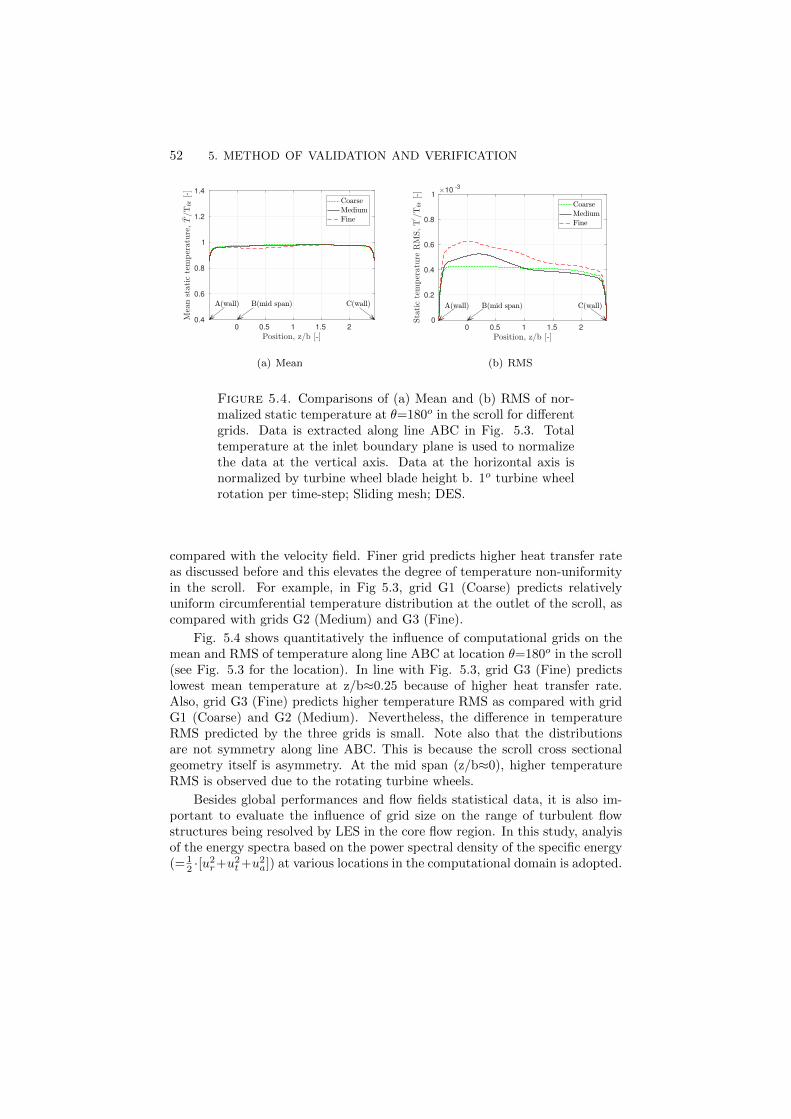
52 5. METHOD OF VALIDATION AND VERIFICATION
0 0.5 1 1.5 2
0.4
0.6
0.8
1
1.2
1.4
(a) Mean
0 0.5 1 1.5 2
0
0.2
0.4
0.6
0.8
110
-3
(b) RMS
Figure 5.4. Comparisons of (a) Mean and (b) RMS of nor-malized static temperature at θ=180o in the scroll for differentgrids. Data is extracted along line ABC in Fig. 5.3. Totaltemperature at the inlet boundary plane is used to normalizethe data at the vertical axis. Data at the horizontal axis isnormalized by turbine wheel blade height b. 1o turbine wheelrotation per time-step; Sliding mesh; DES.
compared with the velocity field. Finer grid predicts higher heat transfer rateas discussed before and this elevates the degree of temperature non-uniformityin the scroll. For example, in Fig 5.3, grid G1 (Coarse) predicts relativelyuniform circumferential temperature distribution at the outlet of the scroll, ascompared with grids G2 (Medium) and G3 (Fine).
Fig. 5.4 shows quantitatively the influence of computational grids on themean and RMS of temperature along line ABC at location θ=180o in the scroll(see Fig. 5.3 for the location). In line with Fig. 5.3, grid G3 (Fine) predictslowest mean temperature at z/b≈0.25 because of higher heat transfer rate.Also, grid G3 (Fine) predicts higher temperature RMS as compared with gridG1 (Coarse) and G2 (Medium). Nevertheless, the difference in temperatureRMS predicted by the three grids is small. Note also that the distributionsare not symmetry along line ABC. This is because the scroll cross sectionalgeometry itself is asymmetry. At the mid span (z/b≈0), higher temperatureRMS is observed due to the rotating turbine wheels.
Besides global performances and flow fields statistical data, it is also im-portant to evaluate the influence of grid size on the range of turbulent flowstructures being resolved by LES in the core flow region. In this study, analyisof the energy spectra based on the power spectral density of the specific energy(= 1
2 ·[u2r+u2t+u2a]) at various locations in the computational domain is adopted.

5.4. GRID CONVERGENCE STUDY 53
0.01 0.1 1
Normalized frequency, f/fbpf [-]
10-10
10-5
100
105
Specificenergy,E(f)[m
4/s
3]
Kolmogorov -5/3
CoarseMediumFine
(a) S1 (scroll tongue)
0.01 0.1 1
Normalized frequency, f/fbpf [-]
10-10
10-5
100
105
Specificenergy,E(f)[m
4/s
3]
Kolmogorov -5/3
CoarseMediumFine
(b) R1 (wheel)
0.01 0.1 1
Normalized frequency, f/fbpf [-]
10-10
10-5
100
105
Specificenergy,E(f)[m
4/s
3]
Kolmogorov -5/3
CoarseMediumFine
(c) S2 (z1 = 0.4D)
0.01 0.1 1
Normalized frequency, f/fbpf [-]
10-10
10-5
100
105
Specificenergy,E(f)[m
4/s
3]
Kolmogorov -5/3
CoarseMediumFine
(d) S3 (z2 = 6D)
Figure 5.5. Comparisons of energy spectra at different lo-cations in the computational domain for different grids. (a)S1 (scroll tongue) (b) R1 (wheel) (c) S2 (z1 = 0.4D) (d) S3
(z2 = 6D). Location of the probe points are indicated by reddots in Fig. 5.1. The energy spectra is represented by powerspectral density based on the time history of specific kineticenergy. Data at horizontal axis is normalized by blade passingfrequency fbpf . Kolmogorov -5/3 slope is included for refer-ence purpose. 1o turbine wheel rotation per time-step; Slidingmesh; DES
For a fully developed and isotropic turbulent flow scenario, the range of the tur-bulent flow structures being resolved is represented by the exhibition of inertialsubrange, i.e. the wider the range of Kolmogorov -5/3 slope in the spectra, thewider the range of resolved turbulent eddies size. From Fig. 5.5(a), 5.5(c) and5.5(d), it can be observed that the considered computational grids are capableof capturing the blade passing frequency (f/fbpf=1) in the stationary region.
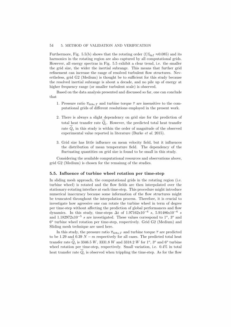
54 5. METHOD OF VALIDATION AND VERIFICATION
Furthermore, Fig. 5.5(b) shows that the rotating order (f/fbpf ≈0.085) and itsharmonics in the rotating region are also captured by all computational grids.However, all energy spectras in Fig. 5.5 exhibit a clear trend, i.e. the smallerthe grid size, the wider the inertial subrange. This means that further gridrefinement can increase the range of resolved turbulent flow structures. Nev-ertheless, grid G2 (Medium) is thought be to sufficient for this study becausethe resolved inertial subrange is about a decade, and no pile up of energy athigher frequency range (or smaller turbulent scale) is observed.
Based on the data analysis presented and discussed so far, one can concludethat
1. Pressure ratio π6t8s,T and turbine torque τ are insensitive to the com-putational grids of different resolutions employed in the present work.
2. There is always a slight dependency on grid size for the prediction of
total heat transfer rate Qt. However, the predicted total heat transfer
rate Qt in this study is within the order of magnitude of the observedexperimental value reported in literature (Burke et al. 2015).
3. Grid size has little influence on mean velocity field, but it influencesthe distribution of mean temperature field. The dependency of thefluctuating quantities on grid size is found to be small in this study.
Considering the available computational resources and observations above,grid G2 (Medium) is chosen for the remainng of the studies.
5.5. Influence of turbine wheel rotation per time-step
In sliding mesh approach, the computational grids in the rotating region (i.e.turbine wheel) is rotated and the flow fields are then interpolated over thestationary-rotating interface at each time-step. This procedure might introducenumerical inaccuracy because some information of the flow structures mightbe truncated throughout the interpolation process. Therefore, it is crucial toinvestigate how agreesive one can rotate the turbine wheel in term of degreeper time-step without affecting the prediction of global performances and flowdynamics. In this study, time-steps ∆t of 1.97162x10⁻⁶ s, 5.91486x10⁻⁶ sand 1.182972x10⁻⁵ s are investigated. These values correspond to 1o, 3o and6o turbine wheel rotation per time-step, respectively. Grid G2 (Medium) andSliding mesh technique are used here.
In this study, the pressure ratio π6t8s,T and turbine torque τ are predictedto be 1.29 and 0.39 N −m respectively for all cases. The predicted total heat
transfer rate Qt is 3346.5 W , 3331.8 W and 3318.2 W for 1o, 3o and 6o turbinewheel rotation per time-step, respectively. Small variation, i.e. 0.4% in total
heat transfer rate Qt is observed when trippling the time-step. As for the flow

5.6. STATIONARY-ROTATING INTERFACE TYPE SENSITIVITY 55
fields, it can be seen from Fig. 5.6, 5.7 and 5.8 that the mean quantities aresimilar for all investigated cases. However, higher fluctuations are predictedwith 1o, whereas 3o and 6o turbine wheel rotation per time-step predict lowerfluctuations at similar level.
The energy spectra for the investigated turbine wheel rotation per time-steps are compared in Fig. 5.9. Comparing with 1o, one can also capture thepeaks of the blade passing frequency and rotating orders by using 3o turbinewheel rotation per time-step. Although with 3o turbine wheel rotation pertime-step, one resolves narrower inertial subrange as compared to 1o in somelocations (e.g. see Fig. 5.9(c)), the Kolmogorov -5/3 slope is still observedup to the blade passing frequency range. Similar phenomenon is not observedwith 6o turbine rotation per time-step.
The data presented and discussed in this section show that
1. Turbine rotation per time-step has insignificant influence on the pres-
sure ratio π6t8s,T , turbine torque τ , total heat transfer rate Qt and meanflow fields.
2. Smaller turbine rotation per time-step predicted larger value of fluctu-ating quantities.
Based on the observations hereinbefore and considering the available com-putational resources, 3o turbine wheel rotation per time-step is thought to besufficient for this study.
5.6. Stationary-rotating interface type sensitivity
Sliding mesh approach is a fully transient approach that can account for theunsteady interaction effects between the rotating turbine wheel and the station-ary scroll tongue. However, this method requires large computational resourcesin terms of simulation time, memory and disk space. An alternative way totreat the turbine wheel rotation is the Frozen rotor technique. In Frozen ro-tor approach, relative positon of the rotating turbine wheel and the stationaryscroll tongue is fixed in time and the conservation of mass, momentum and en-ergy fluxes are maintained across the stationary-rotating interface. AlthoughFrozen rotor method is robust and computational cheaper as compared withthe Sliding mesh approach, it provides only the snapshot solution for the se-lected relative position, Therefore, any attempt to use Frozen rotor techniqueto reduce the computational cost must be done with careful evaluation of itseffects on the global performances and flow field, as compared with Slidingmesh method. In this section, grid G2 (Medium) is used and the turbine wheelis rotated at 3o per time-step.
In this study, it is found that both Sliding mesh and Frozen rotor techniquespredict the same values of pressure ratio π6t8s,T (i.e. 1.29) and turbine torqueτ (i.e. 0.39 N − m). It is worthy to note that the observation about the
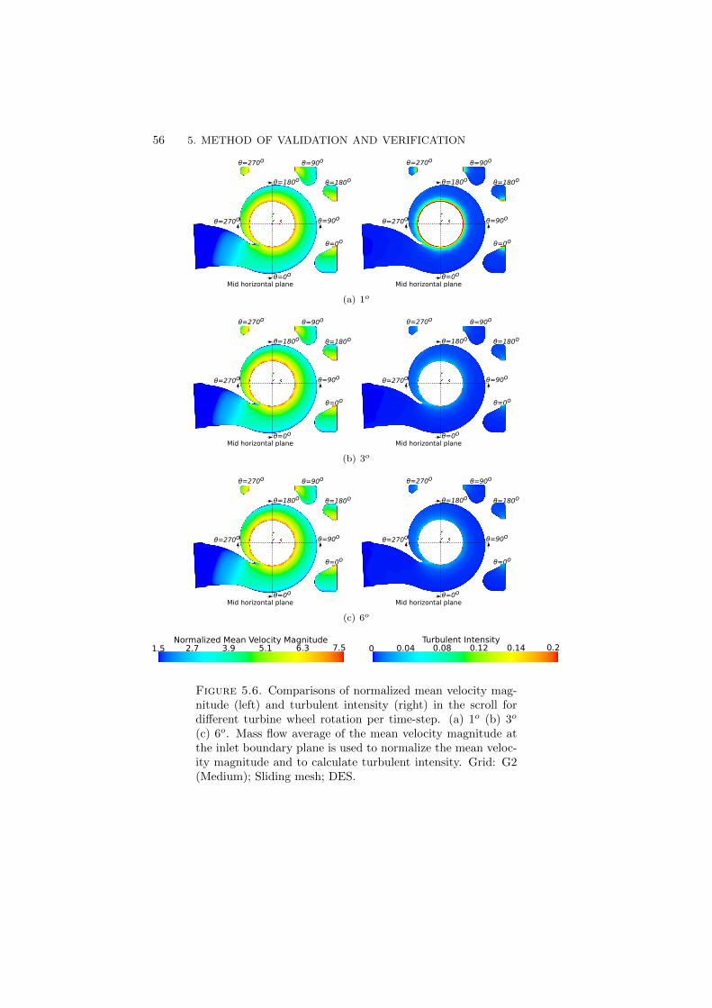
56 5. METHOD OF VALIDATION AND VERIFICATION
θ=0o
θ=90o
θ=180o
θ=270o
θ=0o
θ=90o
θ=180o
θ=270o
Mid horizontal planeθ=0o
θ=90o
θ=180o
θ=270o
θ=0o
θ=90o
θ=180o
θ=270o
Mid horizontal plane
(a) 1o
θ=0o
θ=90o
θ=180o
θ=270o
θ=0o
θ=90o
θ=180o
θ=270o
Mid horizontal planeθ=0o
θ=90o
θ=180o
θ=270o
θ=0o
θ=90o
θ=180o
θ=270o
Mid horizontal plane
(b) 3o
θ=0o
θ=90o
θ=180o
θ=270o
θ=0o
θ=90o
θ=180o
θ=270o
Mid horizontal planeθ=0o
θ=90o
θ=180o
θ=270o
θ=0o
θ=90o
θ=180o
θ=270o
Mid horizontal plane
(c) 6o
Normalized Mean Velocity Magnitude1.5 2.7 3.9 5.1 6.3 7.5
Turbulent Intensity0 0.04 0.08 0.12 0.14 0.2
Figure 5.6. Comparisons of normalized mean velocity mag-nitude (left) and turbulent intensity (right) in the scroll fordifferent turbine wheel rotation per time-step. (a) 1o (b) 3o
(c) 6o. Mass flow average of the mean velocity magnitude atthe inlet boundary plane is used to normalize the mean veloc-ity magnitude and to calculate turbulent intensity. Grid: G2(Medium); Sliding mesh; DES.
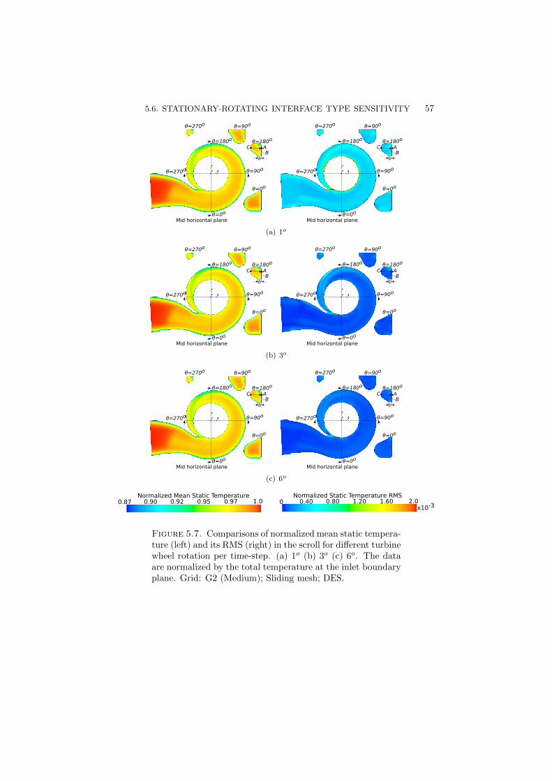
5.6. STATIONARY-ROTATING INTERFACE TYPE SENSITIVITY 57
θ=0o
θ=90o
θ=180o
θ=270o
θ=0o
θ=90o
θ=180o
θ=270o
Mid horizontal planeθ=0o
θ=90o
θ=180o
θ=270o
θ=0o
θ=90o
θ=180o
θ=270o
AC
Mid horizontal plane
b
BAC
b
B
(a) 1o
θ=0o
θ=90o
θ=180o
θ=270o
θ=0o
θ=90o
θ=180o
θ=270o
Mid horizontal planeθ=0o
θ=90o
θ=180o
θ=270o
θ=0o
θ=90o
θ=180o
θ=270o
AC
Mid horizontal plane
b
BAC
b
B
(b) 3o
θ=0o
θ=90o
θ=180o
θ=270o
θ=0o
θ=90o
θ=180o
θ=270o
Mid horizontal plane
AC
b
B
θ=0o
θ=90o
θ=180o
θ=270o
θ=0o
θ=90o
θ=180o
θ=270o
AC
Mid horizontal plane
b
B
(c) 6o
Normalized Mean Static Temperature 0.87 0.90 0.92 0.95 0.97 1.0
Normalized Static Temperature RMS0 0.40 0.80 1.20 1.60 2.0
x10-3
Figure 5.7. Comparisons of normalized mean static tempera-ture (left) and its RMS (right) in the scroll for different turbinewheel rotation per time-step. (a) 1o (b) 3o (c) 6o. The dataare normalized by the total temperature at the inlet boundaryplane. Grid: G2 (Medium); Sliding mesh; DES.
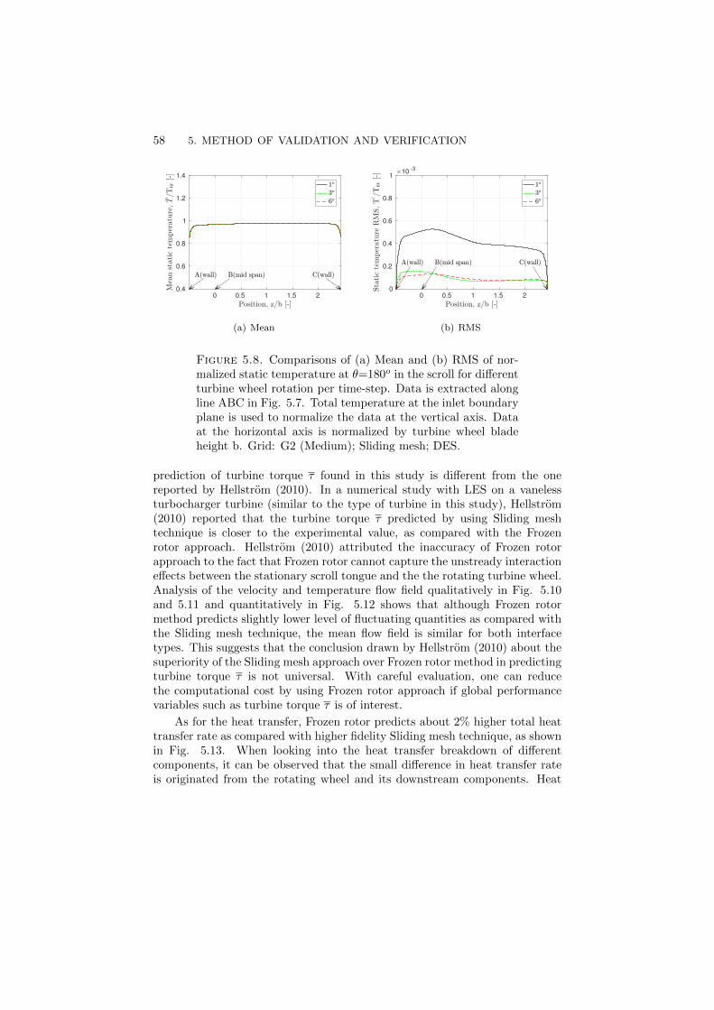
58 5. METHOD OF VALIDATION AND VERIFICATION
0 0.5 1 1.5 2
0.4
0.6
0.8
1
1.2
1.4
(a) Mean
0 0.5 1 1.5 2
0
0.2
0.4
0.6
0.8
110
-3
(b) RMS
Figure 5.8. Comparisons of (a) Mean and (b) RMS of nor-malized static temperature at θ=180o in the scroll for differentturbine wheel rotation per time-step. Data is extracted alongline ABC in Fig. 5.7. Total temperature at the inlet boundaryplane is used to normalize the data at the vertical axis. Dataat the horizontal axis is normalized by turbine wheel bladeheight b. Grid: G2 (Medium); Sliding mesh; DES.
prediction of turbine torque τ found in this study is different from the onereported by Hellstrom (2010). In a numerical study with LES on a vanelessturbocharger turbine (similar to the type of turbine in this study), Hellstrom(2010) reported that the turbine torque τ predicted by using Sliding meshtechnique is closer to the experimental value, as compared with the Frozenrotor approach. Hellstrom (2010) attributed the inaccuracy of Frozen rotorapproach to the fact that Frozen rotor cannot capture the unstready interactioneffects between the stationary scroll tongue and the the rotating turbine wheel.Analysis of the velocity and temperature flow field qualitatively in Fig. 5.10and 5.11 and quantitatively in Fig. 5.12 shows that although Frozen rotormethod predicts slightly lower level of fluctuating quantities as compared withthe Sliding mesh technique, the mean flow field is similar for both interfacetypes. This suggests that the conclusion drawn by Hellstrom (2010) about thesuperiority of the Sliding mesh approach over Frozen rotor method in predictingturbine torque τ is not universal. With careful evaluation, one can reducethe computational cost by using Frozen rotor approach if global performancevariables such as turbine torque τ is of interest.
As for the heat transfer, Frozen rotor predicts about 2% higher total heattransfer rate as compared with higher fidelity Sliding mesh technique, as shownin Fig. 5.13. When looking into the heat transfer breakdown of differentcomponents, it can be observed that the small difference in heat transfer rateis originated from the rotating wheel and its downstream components. Heat

5.6. STATIONARY-ROTATING INTERFACE TYPE SENSITIVITY 59
0.01 0.1 1
Normalized frequency, f/fbpf [-]
10-10
10-5
100
105
Specificenergy,E(f)[m
4/s
3]
Kolmogorov -5/3
∆t=1o
∆t=3o
∆t=6o
(a) S1 (scroll tongue)
0.01 0.1 1
Normalized frequency, f/fbpf [-]
10-10
10-5
100
105
Specificenergy,E(f)[m
4/s
3]
Kolmogorov -5/3
∆t=1o
∆t=3o
∆t=6o
(b) R1 (wheel)
0.01 0.1 1
Normalized frequency, f/fbpf [-]
10-10
10-5
100
105
Specificenergy,E(f)[m
4/s
3]
Kolmogorov -5/3
∆t=1o
∆t=3o
∆t=6o
(c) S2 (z1 = 0.4D)
0.01 0.1 1
Normalized frequency, f/fbpf [-]
10-10
10-5
100
105
Specificenergy,E(f)[m
4/s
3]
Kolmogorov -5/3
∆t=1o
∆t=3o
∆t=6o
(d) S3 (z2 = 6D)
Figure 5.9. Comparisons of energy spectra at different loca-tions in the computational domain for different turbine wheelper time-step. (a) S1 (scroll tongue) (b) R1 (wheel) (c) S2
(z1 = 0.4D) (d) S3 (z2 = 6D). Location of probe points isindicated by red dots in Fig. 5.1. The energy spectra is repre-sented by power spectral density based on the time history ofspecific kinetic energy. Kolmogorov -5/3 slope is included forreference purpose. Grid: G2 (Medium); Sliding mesh; DES.
transfer of the components at the upstream of the turbine wheel (e.g. inlet pipeand scroll) are hardly affected by the choice of rotating-stationary interfacetype.
Fig. 5.14 shows the influence of stationary-rotating interface type on theenergy spectra. Since in Frozen rotor approach, the turbine wheel is not physi-cally rotated relative to the stationary region, peaks associated with the bladepassing frequency and rotating orders are not captured. At stationary region

60 5. METHOD OF VALIDATION AND VERIFICATION
θ=0o
θ=90o
θ=180o
θ=270o
θ=0o
θ=90o
θ=180o
θ=270o
Mid horizontal planeθ=0o
θ=90o
θ=180o
θ=270o
θ=0o
θ=90o
θ=180o
θ=270o
Mid horizontal plane
(a) Sliding mesh
θ=0o
θ=90o
θ=180o
θ=270o
θ=0o
θ=90o
θ=180o
θ=270o
Mid horizontal planeθ=0o
θ=90o
θ=180o
θ=270o
θ=0o
θ=90o
θ=180o
θ=270o
Mid horizontal plane
(b) Frozen rotor
Normalized Mean Velocity Magnitude1.5 2.7 3.9 5.1 6.3 7.5
Turbulent Intensity0 0.04 0.08 0.12 0.14 0.2
Figure 5.10. Comparisons of normalized mean velocity mag-nitude (left) and turbulent intensity (right) in the scroll fordifferent stationary-rotating interface type. (a) Sliding mesh(b) Frozen rotor. Mass flow average of the mean velocity mag-nitude at the inlet boundary plane is used to normalize themean velocity magnitude and to calculate turbulent intensity.Grid: G2 (Medium); 3o turbine wheel rotation per time-step;DES.
closed to the outlet of turbine wheel z1 = 0.4D (see Fig. 5.14(c)), the fluctu-ating energy content at lower frequency range (corresponds to larger turbulenteddies) is predicted to be larger by Frozen rotor technique, as compared withthe Sliding mesh approach. This means that heat transfer is enhanced near
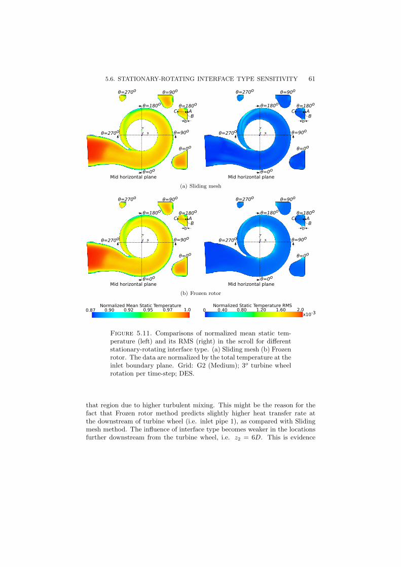
5.6. STATIONARY-ROTATING INTERFACE TYPE SENSITIVITY 61
θ=0o
θ=90o
θ=180o
θ=270o
θ=0o
θ=90o
θ=180o
θ=270o
Mid horizontal planeθ=0o
θ=90o
θ=180o
θ=270o
θ=0o
θ=90o
θ=180o
θ=270o
AC
Mid horizontal plane
b
BAC
b
B
(a) Sliding mesh
θ=0o
θ=90o
θ=180o
θ=270o
θ=0o
θ=90o
θ=180o
θ=270o
Mid horizontal planeθ=0o
θ=90o
θ=180o
θ=270o
θ=0o
θ=90o
θ=180o
θ=270o
AC
Mid horizontal plane
b
BAC
b
B
(b) Frozen rotor
Normalized Mean Static Temperature 0.87 0.90 0.92 0.95 0.97 1.0
Normalized Static Temperature RMS0 0.40 0.80 1.20 1.60 2.0
x10-3
Figure 5.11. Comparisons of normalized mean static tem-perature (left) and its RMS (right) in the scroll for differentstationary-rotating interface type. (a) Sliding mesh (b) Frozenrotor. The data are normalized by the total temperature at theinlet boundary plane. Grid: G2 (Medium); 3o turbine wheelrotation per time-step; DES.
that region due to higher turbulent mixing. This might be the reason for thefact that Frozen rotor method predicts slightly higher heat transfer rate atthe downstream of turbine wheel (i.e. inlet pipe 1), as compared with Slidingmesh method. The influence of interface type becomes weaker in the locationsfurther downstream from the turbine wheel, i.e. z2 = 6D. This is evidence

62 5. METHOD OF VALIDATION AND VERIFICATION
0 0.5 1 1.5 2
0.4
0.6
0.8
1
1.2
1.4
(a) Mean
0 0.5 1 1.5 2
0
0.2
0.4
0.6
0.8
110
-3
(b) RMS
Figure 5.12. Comparisons of (a) Mean and (b) RMS of nor-malized static temperature at θ=180o in the scroll for differentstationary-rotating interface type. Data is extracted along lineABC in Fig. 5.11. Total temperature at the inlet boundaryplane is used to normalize the data at the vertical axis. Dataat the horizontal axis is normalized by turbine wheel bladeheight b. Grid: G2 (Medium); 3o turbine wheel rotation pertime-step; DES.
from Fig. 5.14(d), which shows approximately similar energy spectra for bothapproaches.
Sliding mesh Frozen rotor
Rotating-stationary interface
0
1000
2000
3000
4000
5000
6000
Meanheattran
sfer
rate,¯ Q[W
]
976.5
971.2
805.5
578.6
¯Qt=3331.8
976.9
971.8
829.3
623.7
¯Qt=3401.7
Inlet pipeScrollWheelOutlet pipe 1
Figure 5.13. Comparisons of mean heat transfer rate for dif-ferent components in the computational domain. Grid: G2(Medium); 3o turbine wheel rotation per time-step; DES.

5.6. STATIONARY-ROTATING INTERFACE TYPE SENSITIVITY 63
0.01 0.1 1
Normalized frequency, f/fbpf [-]
10-10
10-5
100
105
Specificenergy,E(f)[m
4/s
3]
Kolmogorov -5/3
Sliding meshFrozen rotor
(a) S1 (scroll tongue)
0.01 0.1 1
Normalized frequency, f/fbpf [-]
10-10
10-5
100
105
Specificenergy,E(f)[m
4/s
3]
Kolmogorov -5/3
Sliding meshFrozen rotor
(b) R1 (wheel)
0.01 0.1 1
Normalized frequency, f/fbpf [-]
10-10
10-5
100
105
Specificenergy,E(f)[m
4/s
3]
Kolmogorov -5/3
Sliding meshFrozen rotor
(c) S2 (z1 = 0.4D)
0.01 0.1 1
Normalized frequency, f/fbpf [-]
10-10
10-5
100
105
Specificenergy,E(f)[m
4/s
3]
Kolmogorov -5/3
Sliding meshFrozen rotor
(d) S3 (z2 = 6D)
Figure 5.14. Comparisons energy spectra at different loca-tions in the computational domain for different stationary-rotating interface type. (a) S1 (scroll tongue) (b) R1 (wheel)(c) S2 (z1 = 0.4D) (d) S3 (z2 = 6D). Locations of probepoints are indicated by red dots in Fig. 5.1. The energy spec-tra is represented by power spectral density based on the timehistory of specific kinetic energy. Kolmogorov -5/3 slope is in-cluded for reference purpose. Grid: G2 (Medium); 3o turbinewheel rotation per time-step; DES.
The data presented and discussed in the study about the influence ofstationary-rotating interface type show that
1. Stationary-rotating interface type has no significant influence on thepredicted results of pressure ratio π6t8s and turbine torque τ in thisstudy. This means that Frozen rotor approach has the potential to re-duce computational cost and it might be useful for iterative industrialdesign and optimization purpose, in which the global performances are
64 5. METHOD OF VALIDATION AND VERIFICATION
of primary interest. In future, it will be useful to investigate also theinfluence of relative position of the turbine wheel and the scroll tonguein Frozen rotor approach.
2. Stationary-rotating interface type has slight influence on the heat trans-fer rate, especially at the downstream of turbine wheel due to differentlevel of predicted turbulent energy content.
3. Stationary-rotating interface type has significant influence on the pre-dicted level of fluctuating energy content, especially at locations near tothe rotating-stationary region interfaces. With Frozen rotor technique,interaction effects of the rotating turbine wheel and the stationary com-ponent cannot be captured.
Although lower fidelity Frozen rotor approach is found to be sufficientin predicting global performances, Sliding mesh technique is chosen for theremaining of the study. This is because besides global performances, analysis ofthe flow structure via mode decompositions will be of interest also in the future.With Frozen rotor technique, coherent flow structures due to fluid-structureinteraction is filtered and it is not suitable in studying the flow dynamics.
5.7. Influence of turbulence model
The comparions of turbine global performances and flow fields between DESand computational cheaper Unsteady RANS (URANS) approach with SSTk − ω turbulence model is presented in this section. The predicted pressureratio π6t8s,T and turbine torque τ are the same for both turbulence models,i.e. 1.29 and 0.39 N − m, respectively. However, DES predicts about 2.3%
higher total heat transfer rate Qt as compared with URANS (i.e. 3331.8 Wand 3256.8 W , respectively). As for the flow fields, it can be seen from Fig.5.15 that the predicted mean velocity field and turbulent intensity are similarfor both turbulence models. Also, comparing to DES, URANS predicts lessnon-uniformity mean temperature distribution at position θ=270o, and thetemperature RMS is predicted to be smoother in the scroll, as shown in Fig.5.16. Quantitatively, it can be observed from Fig. 5.17(a) that there is nosignificant difference in the mean temperature distribution between DES andURANS at the selected position. However, from Fig. 5.17(b), it is clear thatURANS predicts peaks in temperature RMS near the wall, which is in linewith the channel flow experimental results. Those peaks are not observed inDES approach and this might be due to the blending effects as a results ofassuring smooth transition between the RANS and LES region. Further studyis necessary to confirm this.

5.7. INFLUENCE OF TURBULENCE MODEL 65
The energy spectra analysis is depicted in Fig. 5.18. Spectras show thatURANS is more dissipative than DES, as the energy level is damped after theturbine wheel (see Fig. 5.18(c) and 5.18(d)).
Data presented in this section shows that although URANS is as good asDES in predicting the turbine global performances, it is not an appropriateturbulence model to study flow dynamics. Since large scale flow separationsare expected in the turbine operating under engine-like pulsating conditions,DES is thought to be more appropriate in this study. In future, sensitivity ofcomputational solutions to different LES subgrid-scale (SGS) models should beinvestigated to give a more complete view of the influence of turbulence model.
This chapter descibes the computational domain and setup for the tar-geted turbocharger turbine operating under gas stand continuous flow condi-tions. Grid convergence study, influences of turbine wheel rotation per time-step stationary-rotating interface type and turbulence model are investigatedby evaluating the mean global performance variables (pressure ratio π6t8s,T ,
turbine torque τ and total heat transfer rate Qt), flow fields and energy spec-tra. From the studies, grid G2 (Medium) with approximately 9 millions poly-hedral cells and a time-step ∆t corresponds to 3o of turbine wheel rotation arechosen. Sliding mesh technique is chosen to model the rotation of the turbinewheel. Note that the selection is based on the balance between the range offlow structures intended to resolve and the availability of the computationalresources. The selection might not be the optimum one for industrial applica-tions. Nevertheless, the results in this section can serve as valuable guidelinesfor interested party in determining the computational setup, e.g. what infor-mation is gain/loss and how much will it be if a particular configurations ofcomputational setup is chosen.

66 5. METHOD OF VALIDATION AND VERIFICATION
θ=0o
θ=90o
θ=180o
θ=270o
θ=0o
θ=90o
θ=180o
θ=270o
Mid horizontal planeθ=0o
θ=90o
θ=180o
θ=270o
θ=0o
θ=90o
θ=180o
θ=270o
Mid horizontal plane
(a) DES
θ=0o
θ=90o
θ=180o
θ=270o
θ=0o
θ=90o
θ=180o
θ=270o
Mid horizontal planeθ=0o
θ=90o
θ=180o
θ=270o
θ=0o
θ=90o
θ=180o
θ=270o
Mid horizontal plane
(b) URANS
Normalized Mean Velocity Magnitude1.5 2.7 3.9 5.1 6.3 7.5
Turbulent Intensity0 0.04 0.08 0.12 0.14 0.2
Figure 5.15. Comparisons of normalized mean velocity mag-nitude (left) and turbulent intensity (right) in the scroll fordifferent turbulence model. (a) DES (b) URANS. Mass flowaverage of the mean velocity magnitude at the inlet boundaryplane is used to normalize the mean velocity magnitude andas reference level to calculate turbulent intensity. Grid: G2(Medium); 3o turbine wheel rotation per time-step; Slidingmesh.
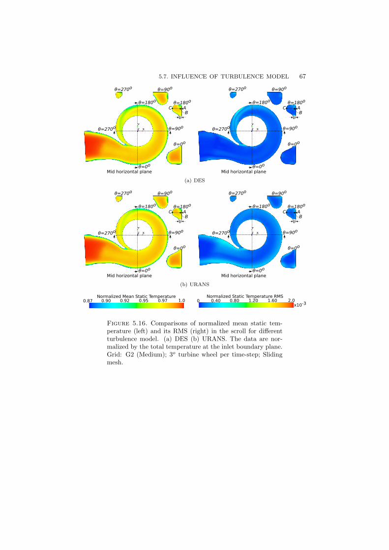
5.7. INFLUENCE OF TURBULENCE MODEL 67
θ=0o
θ=90o
θ=180o
θ=270o
θ=0o
θ=90o
θ=180o
θ=270o
Mid horizontal planeθ=0o
θ=90o
θ=180o
θ=270o
θ=0o
θ=90o
θ=180o
θ=270o
AC
Mid horizontal plane
b
BAC
b
B
(a) DES
θ=0o
θ=90o
θ=180o
θ=270o
θ=0o
θ=90o
θ=180o
θ=270o
Mid horizontal planeθ=0o
θ=90o
θ=180o
θ=270o
θ=0o
θ=90o
θ=180o
θ=270o
AC
Mid horizontal plane
b
BAC
b
B
(b) URANS
Normalized Mean Static Temperature 0.87 0.90 0.92 0.95 0.97 1.0
Normalized Static Temperature RMS0 0.40 0.80 1.20 1.60 2.0
x10-3
Figure 5.16. Comparisons of normalized mean static tem-perature (left) and its RMS (right) in the scroll for differentturbulence model. (a) DES (b) URANS. The data are nor-malized by the total temperature at the inlet boundary plane.Grid: G2 (Medium); 3o turbine wheel per time-step; Slidingmesh.

68 5. METHOD OF VALIDATION AND VERIFICATION
0 0.5 1 1.5 2
0.4
0.6
0.8
1
1.2
1.4
(a) Mean
0 0.5 1 1.5 2
0
0.2
0.4
0.6
0.8
110
-3
(b) RMS
Figure 5.17. Comparisons of (a) Mean and (b) RMS of nor-malized static temperature at θ=180o in the scroll for differentturbulence model. Data is extracted along line ABS in Fig.5.16. Total temperature at the inlet boundary plane is used tonormalize the data at the vertical axis. Data at the horizontalaxis is normalized by turbine wheel blade height b. Grid: G2(Medium); 3o turbine wheel rotation per time-step; Slidingmesh.

5.7. INFLUENCE OF TURBULENCE MODEL 69
0.01 0.1 1
Normalized frequency, f/fbpf [-]
10-10
10-5
100
105
Specificenergy,E(f)[m
4/s
3]
Kolmogorov -5/3
DESURANS
(a) S1 (scroll tongue)
0.01 0.1 1
Normalized frequency, f/fbpf [-]
10-10
10-5
100
105
Specificenergy,E(f)[m
4/s
3]
Kolmogorov -5/3
DESURANS
(b) R1 (wheel)
0.01 0.1 1
Normalized frequency, f/fbpf [-]
10-10
10-5
100
105
Specificenergy,E(f)[m
4/s
3]
Kolmogorov -5/3
DESURANS
(c) S2 (z1 = 0.4D)
0.01 0.1 1
Normalized frequency, f/fbpf [-]
10-10
10-5
100
105
Specificenergy,E(f)[m
4/s
3]
Kolmogorov -5/3
DESURANS
(d) S3 (z2 = 6D)
Figure 5.18. Comparisons of energy spectra at different lo-cations in the computational domain for different turbulencemodel. (a) S1 (scroll tongue) (b) R1 (wheel) (c) S2 (z1 = 0.4D)(d) S3 (z2 = 6D). Locations of probe points are indicated byred dots in Fig. 5.1. The energy spectra is represented bypower spectral density based on the time history of specific ki-netic energy. Kolmogorov -5/3 slope is included for referencepurpose. Grid: G2 (Medium); 3o turbine wheel rotation pertime-step; Sliding mesh.

CHAPTER 6
Heat transfer effects on the turbine performance
This chapter presents and discusses the effects of heat transfer for a tur-bocharger turbine. Two scenarios are considered, namely heat transfer in hotgas stand continuous flow conditions and the engine-like pulsating flow con-ditions. Firstly, the sensitivity of turbine performance to heat transfer levelis investigated by applying the First Law of Thermodynamics to the turbinesystem. Then, the concept of exergy (or availability) based on the Second Lawof Thermodynamics is adopted to quantify the heat transfer related losses inthe turbine system.
6.1. Turbine assessment under continuous flow conditions
In this study, the sensitiviy of turbine performance to different heat trans-fer level is investigated under hot gas stand continuous flow condition. Theheat transfer level is varied by imposing different wall thermal conditions, i.e.adiabatic or constant wall temperatures Tw=1002 K, 830 K and 487 K. Asmentioned in Sec. 5.2, Tw=1002 K is estimated from literature experimentaldata (Romagnoli & Martinez-Botas 2012a) and therefore it represents a morerealistic (but not perfect due to experiment limitations) thermal boundary con-dition in a turbocharger turbine operating in hot gas stand. Tw=830 K and 487K mimic the condition of larger turbine heat loss because of larger temperaturedifference between the hot gas and the wall.
The computational domain and boundary conditions (i.e. min=mT=0.058kg/s, Tt,in=T6t=1173.15 K, ω=84533 rpm) are the same as discussed in Sec.5.1 and 5.2, respectively in Chap. 5. Similarly, the computational setup isas described in Chap. 5, i.e. grid G2 (Medium) with approximately 9 milionpolyhedral cells, sliding mesh technique with 3 degrees of turbine wheel rotationper time-step and SST k − ω Detached Eddy Simulation (DES) turbulencemodel.
Fig. 6.1 shows the sensitivity of mean global performances in terms ofpressure ratio and turbine power to total heat loss. The data at the verticalaxis is normalized by the corresponding adiabatic value to show the deviationof non-adiabatic to adiabatic performance. At the horizontal axis, total heatloss is normalized by the turbine power. No significant change of pressure ratio
70

6.1. TURBINE ASSESSMENT UNDER CONTINUOUS FLOW CONDITIONS 71
0 2 4 6
0.8
0.85
0.9
0.95
1
1.05
Figure 6.1. Turbine performance sensitivity to heat loss un-der hot gas stand continuous flow conditions. Data at the ver-tical axis and horizontal axis is normalized by the adiabaticvalue and turbine power, respectively.
π6t8s,T is observed up to Qt
WT
≈ 1, and then the pressure ratio π6t8s,T drops
linearly as the amount of heat loss increases. On the other hand, the turbine
power WT drops immediately in a linear trend whenever there is heat transfer.This observation is consistent with the theoretical discussions about the effectsof heat transfer on turbine performance in Sec. 2.1.1. Although no significant
change in pressure field is observed up to Qt
WT
≈ 1, the static temperature
at the turbine wheel inlet is lowered due to heat transfer. Furthermore, itcan be seen from Fig. 6.1 that turbine power has steeper slope, as comparedwith the pressure ratio. This means that turbine power is more sensitive toheat loss, as compared with the pressure ratio. This shows that there is arisk to draw inappropriate conclusions about the influence of heat transfer onthe aerothermodynamics of turbine by just comparing the pressure ratio inadiabatic and non-adiabatic scenarios.
The discussions above are based on energy balance analysis, i.e. first law ofthermodynamics. One drawback of the energy balance analysis is its inabilityto identify and quantify the mechanisms of heat transfer related losses. In orderto identify and quantify the heat transfer related losses, an exergy analysis isperformed base on the CFD data. Fig. 6.2 depicts the exergy budget of eachsystem component (i.e. inlet pipe, scroll, wheel, outlet pipe 1) in the turbinesystem for different heat transfer level. Each stacked bar represents a single

72 6. HEAT TRANSFER EFFECTS ON THE TURBINE PERFORMANCE
heat transfer scenario. Note that instead of wall temperature Tw, ToTw
is usedto represents the non-adiabatic scenario in the exergy budget to show how farthe system boundary temperature is away from the dead state temperatureTo =298.15 K. The larger the value of To
Tw, the larger the amount of heat loss.
The total height of the stacked bar is the time derivative of flow exergy in amaterial control volume (see Sec. 2.6), normalized by the inflow exergy at theinlet boundary place. Overline denotes the mean value. The stacked bar canbe further broken down into a few components, which tell us the mechanismsresponsible for exergy change within the system component (see Sec. 2.6 for
details of exergy). Heat transported exergy∑
(1− ToTw )Q
ias denoted by red
color can be considered as a kind loss also because it cannot be further utilizedfor useful work.
From Fig. 6.2, it can be observed that for all system components, heat loss
increases the heat transported exergy∑
(1− ToTw )Q
i, as expected. Similarly,
thermal irreversibility Ithermal also increases due to larger temperature gradient
as a result of heat transfer. On the other hand, viscous irreversibility Iviscousremains relatively small although the amount of heat loss increases. As for theturbine power, it follows the same trend as discussed before, i.e. linear dropwith heat loss. The rate of pressure accumulation within the system componentddt
˝V ∗(t)
pdV denoted by magenta color is relatively very small as compared
with other components and it is hardly visible in Fig. 6.2. This indicates thatddt
˝V ∗(t)
pdV term is insignicant as compared with other terms and one might
want to perform exergy analysis based on steady RANS CFD data in order toreduce computational cost. Note that this alternative is only possible for hotgas stand continuous flow condition. For engine-like pulsating flow scenario,transient simulation is still necessary due to time varying boundary conditions.
In order to assess how well the turbine system utilizes the available energyresource (i.e. exergy), overall exergy budget for different heat transfer levelcan be plotted, as depicted in Fig. 6.3(a). Note that the maximum of thenormalized value in the vertical axis is one, which represents the upper limitof the exergy that can be extracted by the system. From Fig. 6.3(a), it canbe seen that with heat transfer, although much of the exergy is destroyed viairreversibilities and heat transport, the drop in turbine power observed fromenergy balance analysis is only a small portion of the total exergy. Even in themost ideal situation (i.e. adiabatic), the turbine can only extract about 10% ofthe available energy to the system. This indicates that much of the exergy is notutilized in the turbine system. The non-utilized exergy is totally dischargedout from the turbine system as high temperature hot gas in the adiabaticscenario. With heat transfer, part of the exergy is discharged out from theturbine system as lower temperature gas, and part of the exergy is destroyed
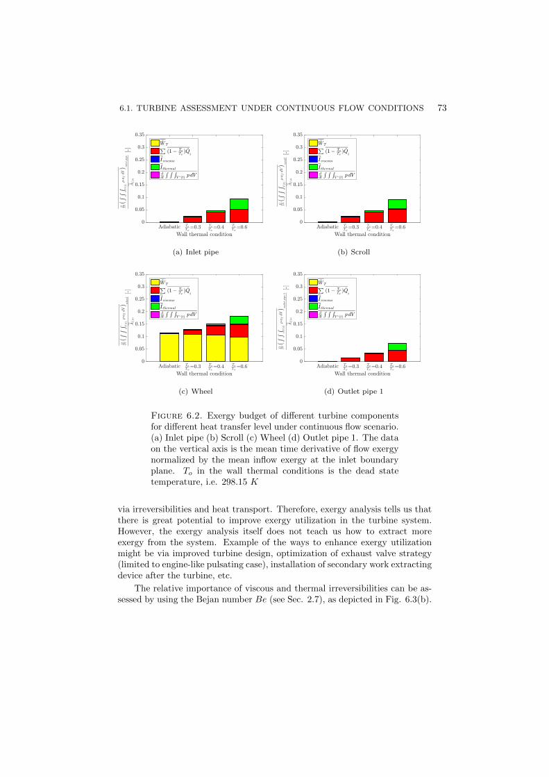
6.1. TURBINE ASSESSMENT UNDER CONTINUOUS FLOW CONDITIONS 73
(a) Inlet pipe (b) Scroll
(c) Wheel (d) Outlet pipe 1
Figure 6.2. Exergy budget of different turbine componentsfor different heat transfer level under continuous flow scenario.(a) Inlet pipe (b) Scroll (c) Wheel (d) Outlet pipe 1. The dataon the vertical axis is the mean time derivative of flow exergynormalized by the mean inflow exergy at the inlet boundaryplane. To in the wall thermal conditions is the dead statetemperature, i.e. 298.15 K
via irreversibilities and heat transport. Therefore, exergy analysis tells us thatthere is great potential to improve exergy utilization in the turbine system.However, the exergy analysis itself does not teach us how to extract moreexergy from the system. Example of the ways to enhance exergy utilizationmight be via improved turbine design, optimization of exhaust valve strategy(limited to engine-like pulsating case), installation of secondary work extractingdevice after the turbine, etc.
The relative importance of viscous and thermal irreversibilities can be as-sessed by using the Bejan number Be (see Sec. 2.7), as depicted in Fig. 6.3(b).
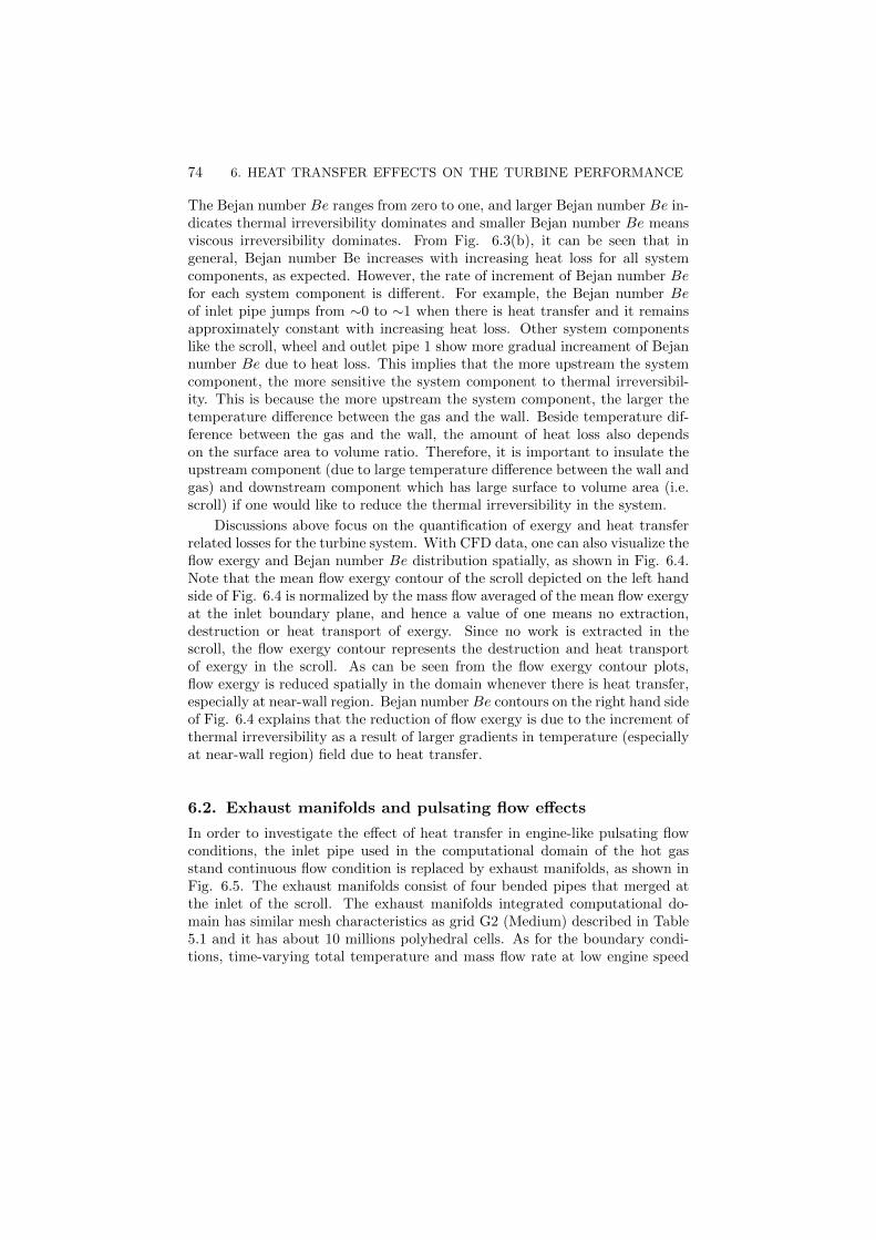
74 6. HEAT TRANSFER EFFECTS ON THE TURBINE PERFORMANCE
The Bejan number Be ranges from zero to one, and larger Bejan number Be in-dicates thermal irreversibility dominates and smaller Bejan number Be meansviscous irreversibility dominates. From Fig. 6.3(b), it can be seen that ingeneral, Bejan number Be increases with increasing heat loss for all systemcomponents, as expected. However, the rate of increment of Bejan number Befor each system component is different. For example, the Bejan number Beof inlet pipe jumps from ∼0 to ∼1 when there is heat transfer and it remainsapproximately constant with increasing heat loss. Other system componentslike the scroll, wheel and outlet pipe 1 show more gradual increament of Bejannumber Be due to heat loss. This implies that the more upstream the systemcomponent, the more sensitive the system component to thermal irreversibil-ity. This is because the more upstream the system component, the larger thetemperature difference between the gas and the wall. Beside temperature dif-ference between the gas and the wall, the amount of heat loss also dependson the surface area to volume ratio. Therefore, it is important to insulate theupstream component (due to large temperature difference between the wall andgas) and downstream component which has large surface to volume area (i.e.scroll) if one would like to reduce the thermal irreversibility in the system.
Discussions above focus on the quantification of exergy and heat transferrelated losses for the turbine system. With CFD data, one can also visualize theflow exergy and Bejan number Be distribution spatially, as shown in Fig. 6.4.Note that the mean flow exergy contour of the scroll depicted on the left handside of Fig. 6.4 is normalized by the mass flow averaged of the mean flow exergyat the inlet boundary plane, and hence a value of one means no extraction,destruction or heat transport of exergy. Since no work is extracted in thescroll, the flow exergy contour represents the destruction and heat transportof exergy in the scroll. As can be seen from the flow exergy contour plots,flow exergy is reduced spatially in the domain whenever there is heat transfer,especially at near-wall region. Bejan number Be contours on the right hand sideof Fig. 6.4 explains that the reduction of flow exergy is due to the increment ofthermal irreversibility as a result of larger gradients in temperature (especiallyat near-wall region) field due to heat transfer.
6.2. Exhaust manifolds and pulsating flow effects
In order to investigate the effect of heat transfer in engine-like pulsating flowconditions, the inlet pipe used in the computational domain of the hot gasstand continuous flow condition is replaced by exhaust manifolds, as shown inFig. 6.5. The exhaust manifolds consist of four bended pipes that merged atthe inlet of the scroll. The exhaust manifolds integrated computational do-main has similar mesh characteristics as grid G2 (Medium) described in Table5.1 and it has about 10 millions polyhedral cells. As for the boundary condi-tions, time-varying total temperature and mass flow rate at low engine speed
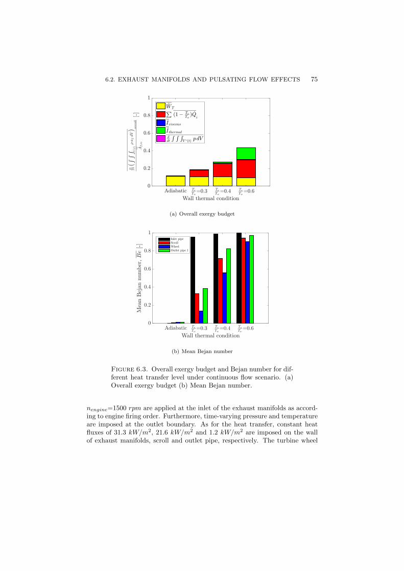
6.2. EXHAUST MANIFOLDS AND PULSATING FLOW EFFECTS 75
(a) Overall exergy budget
Adiabatic To
Tw
=0.3 To
Tw
=0.4 To
Tw
=0.6
Wall thermal condition
0
0.2
0.4
0.6
0.8
1
MeanBejan
number,Be[-]
Inlet pipeScrollWheelOutlet pipe 1
(b) Mean Bejan number
Figure 6.3. Overall exergy budget and Bejan number for dif-ferent heat transfer level under continuous flow scenario. (a)Overall exergy budget (b) Mean Bejan number.
nengine=1500 rpm are applied at the inlet of the exhaust manifolds as accord-ing to engine firing order. Furthermore, time-varying pressure and temperatureare imposed at the outlet boundary. As for the heat transfer, constant heatfluxes of 31.3 kW/m2, 21.6 kW/m2 and 1.2 kW/m2 are imposed on the wallof exhaust manifolds, scroll and outlet pipe, respectively. The turbine wheel

76 6. HEAT TRANSFER EFFECTS ON THE TURBINE PERFORMANCE
θ=0o
θ=90o
θ=180o
θ=270o
θ=0o
θ=90o
θ=180o
θ=270o
Mid horizontal planeθ=0o
θ=90o
θ=180o
θ=270o
θ=0o
θ=90o
θ=180o
θ=270o
Mid horizontal plane
(a) Adiabatic
θ=0o
θ=90o
θ=180o
θ=270o
θ=0o
θ=90o
θ=180o
θ=270o
Mid horizontal planeθ=0o
θ=90o
θ=180o
θ=270o
θ=0o
θ=90o
θ=180o
θ=270o
Mid horizontal plane
(b) To/Tw=0.3
θ=0o
θ=90o
θ=180o
θ=270o
θ=0o
θ=90o
θ=180o
θ=270o
Mid horizontal planeθ=0o
θ=90o
θ=180o
θ=270o
θ=0o
θ=90o
θ=180o
θ=270o
Mid horizontal plane
(c) To/Tw=0.4
θ=0o
θ=90o
θ=180o
θ=270o
θ=0o
θ=90o
θ=180o
θ=270o
Mid horizontal planeθ=0o
θ=90o
θ=180o
θ=270o
θ=0o
θ=90o
θ=180o
θ=270o
Mid horizontal plane
(d) To/Tw=0.6
Normalized Mean Flow Exergy 0 0.20 0.40 0.60 0.80 1.0
Mean Bejan Number0 0.20 0.40 0.60 0.80 1.0
Figure 6.4. Comparisons of normalized mean flow exergy(left) and mean Bejan number (right) in the scroll for differentheat transfer level under continuous flow scenario. (a) Adia-batic (b) To/Tw=0.3 (c) To/Tw=0.4 (d) To/Tw=0.6. Mass flowaverage of the mean flow exergy at the inlet boundary planeis used to normalize the mean flow exergy.

6.2. EXHAUST MANIFOLDS AND PULSATING FLOW EFFECTS 77
2
3
4
1
Figure 6.5. Computational domain for engine-like pulsatingflow conditions. Time varying boundary conditions as accord-ing to the engine firing order obtained from engine calibratedone-dimensional model are imposed.
is treated as adiabatic and rotating at varying speed. The aforementionedboundary conditions (provided by industrial partner) are obtained from theengine calibrated one-dimensional model, which represent the on-engine con-ditions. An additional case with all system components treated as adiabatic isalso setup to study the influence of heat transfer on turbine performance underengine-like pulsating condition.
As for the computation setup, similar to Sec. 6.1, sliding mesh techniquewith a constant time-step equivalent to 3 degrees of turbine wheel rotation pertime-step is used. The constant time-step is derived from the mean of the time-varying turbine speed. SST k−ω Detached Eddy Simulation (DES) turbulencemodel is used. Prior to the transient simulations, the mean value of time-varying boundary conditions is imposed and steady-state RANS is performedwith mixing plane interface between the stationary and rotating region. Thesteady-state RANS data is then used to initialize the flow field of the transient
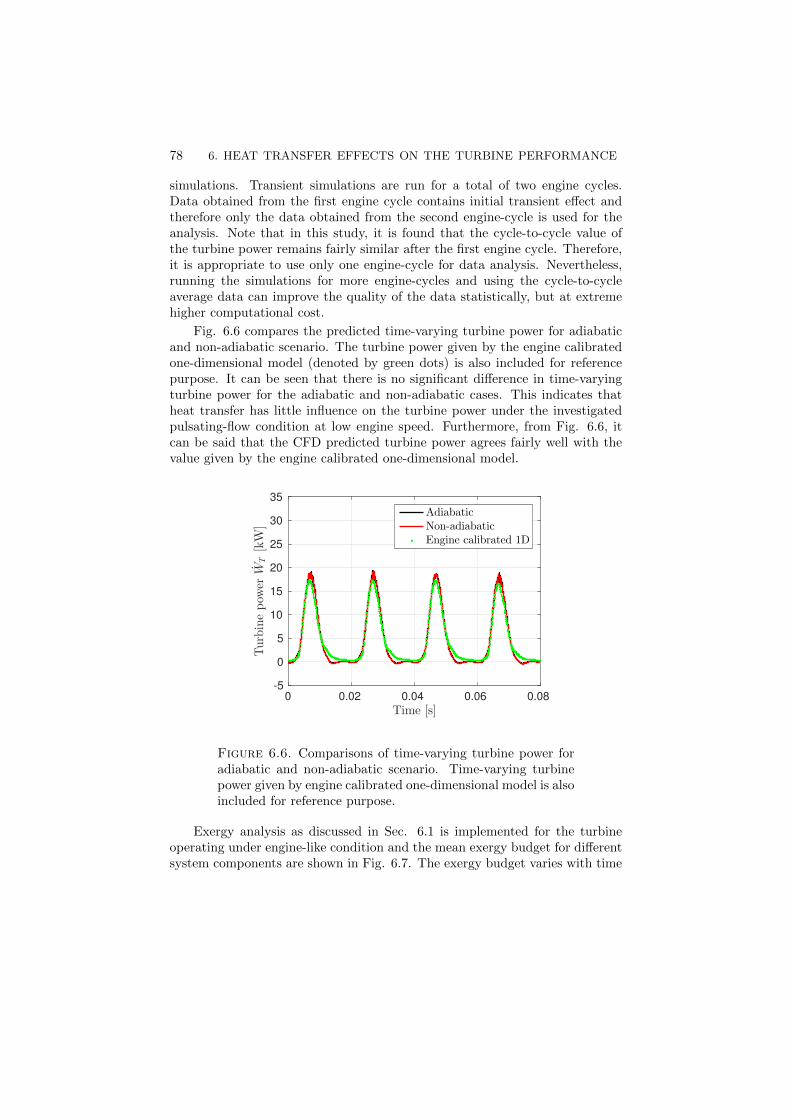
78 6. HEAT TRANSFER EFFECTS ON THE TURBINE PERFORMANCE
simulations. Transient simulations are run for a total of two engine cycles.Data obtained from the first engine cycle contains initial transient effect andtherefore only the data obtained from the second engine-cycle is used for theanalysis. Note that in this study, it is found that the cycle-to-cycle value ofthe turbine power remains fairly similar after the first engine cycle. Therefore,it is appropriate to use only one engine-cycle for data analysis. Nevertheless,running the simulations for more engine-cycles and using the cycle-to-cycleaverage data can improve the quality of the data statistically, but at extremehigher computational cost.
Fig. 6.6 compares the predicted time-varying turbine power for adiabaticand non-adiabatic scenario. The turbine power given by the engine calibratedone-dimensional model (denoted by green dots) is also included for referencepurpose. It can be seen that there is no significant difference in time-varyingturbine power for the adiabatic and non-adiabatic cases. This indicates thatheat transfer has little influence on the turbine power under the investigatedpulsating-flow condition at low engine speed. Furthermore, from Fig. 6.6, itcan be said that the CFD predicted turbine power agrees fairly well with thevalue given by the engine calibrated one-dimensional model.
0 0.02 0.04 0.06 0.08
Time [s]
-5
0
5
10
15
20
25
30
35
Turbinepow
erW
T[kW
]
AdiabaticNon-adiabaticEngine calibrated 1D
Figure 6.6. Comparisons of time-varying turbine power foradiabatic and non-adiabatic scenario. Time-varying turbinepower given by engine calibrated one-dimensional model is alsoincluded for reference purpose.
Exergy analysis as discussed in Sec. 6.1 is implemented for the turbineoperating under engine-like condition and the mean exergy budget for differentsystem components are shown in Fig. 6.7. The exergy budget varies with time
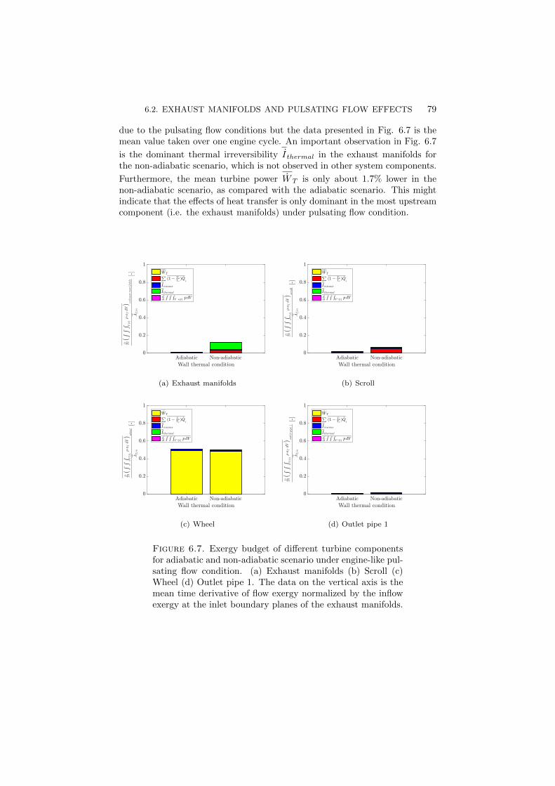
6.2. EXHAUST MANIFOLDS AND PULSATING FLOW EFFECTS 79
due to the pulsating flow conditions but the data presented in Fig. 6.7 is themean value taken over one engine cycle. An important observation in Fig. 6.7
is the dominant thermal irreversibility Ithermal in the exhaust manifolds forthe non-adiabatic scenario, which is not observed in other system components.
Furthermore, the mean turbine power WT is only about 1.7% lower in thenon-adiabatic scenario, as compared with the adiabatic scenario. This mightindicate that the effects of heat transfer is only dominant in the most upstreamcomponent (i.e. the exhaust manifolds) under pulsating flow condition.
(a) Exhaust manifolds (b) Scroll
(c) Wheel (d) Outlet pipe 1
Figure 6.7. Exergy budget of different turbine componentsfor adiabatic and non-adiabatic scenario under engine-like pul-sating flow condition. (a) Exhaust manifolds (b) Scroll (c)Wheel (d) Outlet pipe 1. The data on the vertical axis is themean time derivative of flow exergy normalized by the inflowexergy at the inlet boundary planes of the exhaust manifolds.

80 6. HEAT TRANSFER EFFECTS ON THE TURBINE PERFORMANCE
As for the utilization of flow exergy in the pulsating flow turbine system,it can be seen from the overall exergy budget in Fig. 6.8(a) that turbinepower only accounts for ∼50% of the total inflow exergy. There is still ∼30%of flow exergy that can potentially be extracted as useful work even undernon-adiabatic scenario. This indicates that there might be options to enhanceexergy utilization via improved turbine design, optimization of exhaust valvestrategy, etc.
Looking at the Bejan number Be for different system component in Fig.6.8(b), one can say that thermal irreversibility plays an important part in thetotal irreverbilities in the exhaust manifolds even in the adiabatic scenario.This might be due to large gradients in the temperature field as a result of flowinstabilities in the exhaust manifolds.

6.2. EXHAUST MANIFOLDS AND PULSATING FLOW EFFECTS 81
(a) Overall exergy budget
(b) Mean Bejan number
Figure 6.8. Overall exergy budget and Bejan number for adi-abatic and non-adiabatic scenarios under engine-like pulsatingflow condition. (a) Overall exergy budget (b) Mean Bejannumber.
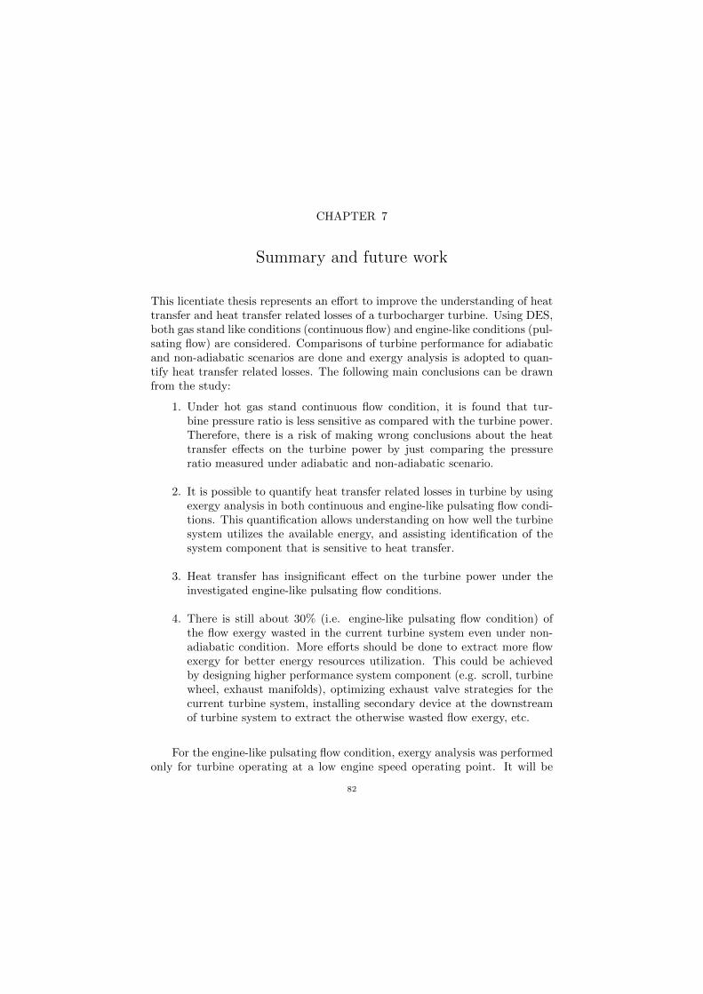
CHAPTER 7
Summary and future work
This licentiate thesis represents an effort to improve the understanding of heattransfer and heat transfer related losses of a turbocharger turbine. Using DES,both gas stand like conditions (continuous flow) and engine-like conditions (pul-sating flow) are considered. Comparisons of turbine performance for adiabaticand non-adiabatic scenarios are done and exergy analysis is adopted to quan-tify heat transfer related losses. The following main conclusions can be drawnfrom the study:
1. Under hot gas stand continuous flow condition, it is found that tur-bine pressure ratio is less sensitive as compared with the turbine power.Therefore, there is a risk of making wrong conclusions about the heattransfer effects on the turbine power by just comparing the pressureratio measured under adiabatic and non-adiabatic scenario.
2. It is possible to quantify heat transfer related losses in turbine by usingexergy analysis in both continuous and engine-like pulsating flow condi-tions. This quantification allows understanding on how well the turbinesystem utilizes the available energy, and assisting identification of thesystem component that is sensitive to heat transfer.
3. Heat transfer has insignificant effect on the turbine power under theinvestigated engine-like pulsating flow conditions.
4. There is still about 30% (i.e. engine-like pulsating flow condition) ofthe flow exergy wasted in the current turbine system even under non-adiabatic condition. More efforts should be done to extract more flowexergy for better energy resources utilization. This could be achievedby designing higher performance system component (e.g. scroll, turbinewheel, exhaust manifolds), optimizing exhaust valve strategies for thecurrent turbine system, installing secondary device at the downstreamof turbine system to extract the otherwise wasted flow exergy, etc.
For the engine-like pulsating flow condition, exergy analysis was performedonly for turbine operating at a low engine speed operating point. It will be
82

7. SUMMARY AND FUTURE WORK 83
interesting to adopt similar methodology to other engine operating conditionslike medium engine speed and maximum engine power in the future to have acomplete picture of heat transfer effects on the turbine performance. Further-more, post-processing techniques like Proper Orthogonal Mode Decomposition(POD) and Dynamic Mode Decomposition (DMD) could be applied to investi-gate the most energetic flow structures and the flow instabilities. As mentioned,exergy analysis indicates that much of the flow exergy is wasted in the currentturbine system. Therefore, future work will focus on exploring different ex-haust valve strategies to reduce losses and to optimize flow exergy extractionas useful turbine work to improve utilization of exhaust gas exergy.

Acknowledgements
This study was performed within the framework of the Competence Centerfor Gas Exchange (CCGEx) at KTH. Firstly, I acknowledge the supports andcontributions from Scania, Volvo GTT, Volvo Cars, Swedish Energy Agencyand BorgWarner. The Swedish National Infrastructure for Computing via Par-allel Computing Center (PDC) at KTH is also acknowledged for providing thecomputational resources.
Secondly, I would like to express my deepest gratitude to my main super-visor, Mihai Mihaescu for entrusting me to work on the project, sharing hisCFD expertise throughout the setup of the computational cases and giving mevaluable comments on my scientific writings. I also appreciate your efforts incoordinating regular research meetings with the industrial partners, which giveme the chance to understand the research questions in automotive industry.Your effort in gathering the expertises from theoretical to applied fluid me-chanics into the supervising board is also highly appreciated because it enablesme access to various resources for consultations when I face difficulties in theproject.
I am also thankful to Anders Dahlkild for proposing to use exergy concept,which forms the core of this licentiate thesis, to analyze heat transfer problemin turbine. Your guidance in deriving the unsteady exergy equations from thefundamental and interpretation of the exergy analysis results is highly appreci-ated. Through your lectures and our regular discussions, I have also strenghtenmy fundamental understanding of fluid mechanics and thermodynamics. I alsoappretiate your great help in translating the abstract of this thesis from Englishto Swedish.
Christophe Duwig and Laszlo Fuchs are also greatly acknowledged for theirconstructive and critical comments during the presentations within the researchgroup. Your comments are always challenging and they inspire me to dig deepinto the basic to search for the truth of science.
Jens Fransson is thanked for giving me ideas to improve the readability ofthe licentiate thesis.
84

ACKNOWLEDGEMENTS 85
Special thanks to Henrik Alfredsson for the wonderful compressible floworal examination. The experience motivates me to improve my scientific dis-cussion skills in terms of clearness and preciseness continuously.
I also thank Bertrand Kerres, Elias Sundstrom and Romain Gojon for theirvaluable comments and fruitful discussions about my research results duringthe turbomachinery and compressible flow group meeting. Fredrik Johnsson isalso thanked for sharing his expertise in helping me to understand how one-dimensional engine modeling data should be interpreted. Lukas Schickhofer’sefforts to be my virtual opponent for the licentiate seminar rehearsal is alsohighly appreciated.
Last but not least, I would like to thank my wife, Sachiko for her endlesssupports while I am pursuing my career as a researcher. I benefit from ourdiscussions about presentation techniques as your ideas and comments alwayslead to successful presentation during my career. Moreover, I am grateful tomy children, Sofia and Frederik for reminding me the importance of curiosityin pursuing knowledge by always asking why when observing daily life phenom-enon.

References
Aghaali, H. & Angstrom, H.-E. 2012 Improving turbocharged engine simulationby including heat transfer in the turbocharger. In SAE Technical Paper . SAEInternational.
Aghaali, H., Angstrom, H.-E. & Serrano, J. R. 2015 Evaluation of differentheat transfer conditions on an automotive turbocharger. International Journalof Engine Research 16 (2), 137–151.
An, F., Earley, R. & Green-Weiskel, L. 2011 Global overview on fuel efficiencyand motor vehicle emission standards: policy options and perspectives for inter-national cooperation. United Nations Background Paper (3).
Baines, N. 2005 Fundamentals of Turbocharging . Concepts NREC.
Baines, N., Wygant, K. D. & Dris, A. 2010 The analysis of heat transfer inautomotive turbochargers. Journal of Engineering for Gas Turbines and Power132 (4), 042301.
Bejan, A. 1995 Entropy generation minimization: the method of thermodynamicoptimization of finite-size systems and finite-time processes. CRC press.
Bohn, D., Heuer, T. & Kusterer, K. 2005 Conjugate flow and heat transferinvestigation of a turbo charger. Journal of engineering for gas turbines andpower 127 (3), 663–669.
Burke, R., Vagg, C., Chalet, D. & Chesse, P. 2015 Heat transfer in turbochargerturbines under steady, pulsating and transient conditions. International Journalof Heat and Fluid Flow 52, 185–197.
Car Throttle 2013 The difference between turbos and su-perchargers explained. https://www.carthrottle.com/post/
the-difference-between-turbos-superchargers-explained/.
Celik, I. B., Ghia, U., Roache, P. J. et al. 2008 Procedure for estimation andreporting of uncertainty due to discretization in CFD applications. Journal offluids Engineering-Transactions of the ASME 130 (7).
Chesse, P., Chalet, D. & Tauzia, X. 2011 Impact of the heat transfer on theperformance calculations of automotive turbocharger compressor. Oil & GasScience and Technology–Revue dIFP Energies nouvelles 66 (5), 791–800.
86
REFERENCES 87
Chow, P., Cross, M. & Pericleous, K. 1996 A natural extension of the conven-tional finite volume method into polygonal unstructured meshes for cfd applica-tion. Applied Mathematical Modelling 20 (2), 170 – 183.
Cohen, I. & Kundu, P. 2007 Fluid Mechanics. Elsevier Science.
Cormerais, M., Chesse, P. & Hetet, J.-F. 2009 Turbocharger heat transfer mod-eling under steady and transient conditions. International Journal of Thermo-dynamics 12 (4), 193.
Cormerais, M., Hetet, J. F., Chesse, P. & Maiboom, A. 2006 Heat trans-fer analysis in a turbocharger compressor: Modeling and experiments. In SAETechnical Paper . SAE International.
Galindo, J., Fajardo, P., Navarro, R. & Garca-Cuevas, L. 2013 Characteri-zation of a radial turbocharger turbine in pulsating flow by means of CFD andits application to engine modeling. Applied Energy 103, 116 – 127.
Germano, M., Piomelli, U., Moin, P. & Cabot, W. H. 1991 A dynamic subgrid-scale eddy viscosity model. Physics of Fluids A: Fluid Dynamics (1989-1993)3 (7), 1760–1765.
Gourdain, N., Sicot, F., Duchaine, F. & Gicquel, L. 2014 Large eddy simula-tion of flows in industrial compressors: a path from 2015 to 2035. PhilosophicalTransactions of the Royal Society of London A: Mathematical, Physical and En-gineering Sciences 372 (2022).
Gritskevich, M. S., Garbaruk, A. V., Schutze, J. & Menter, F. R. 2012Development of ddes and iddes formulations for the k-ω shear stress transportmodel. Flow, turbulence and combustion 88 (3), 431–449.
Hah, C. 2009 Large eddy simulation of transonic flow field in NASA rotor 37 . Na-tional Aeronautics and Space Administration, Glenn Research Center.
He, L. & Oldfield, M. 2011 Unsteady conjugate heat transfer modeling. Journalof turbomachinery 133 (3), 031022.
Hellstrom, F. 2010 Numerical computations of the unsteady flow in turbochargers.Stockholm: KTH.
Hellstrom, F. & Fuchs, L. 2010 Assessment of heat transfer effects on the per-formance of a radial turbine using large eddy simulation. In 9th InternationalConference on Turbochargers and Turbocharging; Westminster, London; UnitedKingdom; 19 May 2010 through 20 May 2010 , pp. 281–291.
Heywood, J. 1988 Internal Combustion Engine Fundamentals. McGraw-Hill.
Honeywell International Inc. 2016 How a turbo system works. https://www.turbobygarrett.com/turbobygarrett/basic.
International Energy Agency 2012 Fuel economy of road vehicles .
International Energy Agency 2016 Global EV outlook 2016. beyond one millionelectric cars .
Jarrin, N., Benhamadouche, S., Laurence, D. & Prosser, R. 2006 A synthetic-eddy-method for generating inflow conditions for large-eddy simulations. Inter-national Journal of Heat and Fluid Flow 27 (4), 585 – 593, special Issue of TheFourth International Symposium on Turbulence and Shear Flow Phenomena -2005Special Issue of The Fourth International Symposium on Turbulence andShear Flow Phenomena - 2005.

88 REFERENCES
Jung, M., Ford, R. G., Glover, K., Collings, N., Christen, U. & Watts,M. J. 2002 Parameterization and transient validation of a variable geometryturbocharger for mean-value modeling at low and medium speed-load points. InSAE Technical Paper . SAE International.
Karamavruc, A. 2016 Obtaining bulk flow based heat transfer coefficients for ther-mal evaluation of turbochargers. In 12th international conference on turbocharg-ers and turbocharging . Institution of Mechanical Engineers.
Launder, B. E. & Spalding, D. 1974 The numerical computation of turbulentflows. Computer methods in applied mechanics and engineering 3 (2), 269–289.
Leonard, T., Gicquel, L. Y., Gourdain, N. & Duchaine, F. 2015Steady/unsteady reynolds-averaged navier–stokes and large eddy simulations ofa turbine blade at high subsonic outlet mach number. Journal of Turbomachinery137 (4), 041001.
Menter, F. 1992 Influence of freestream values on k-omega turbulence model pre-dictions. AIAA journal 30 (6), 1657–1659.
Menter, F. & Kuntz, M. 2004 Adaptation of eddy-viscosity turbulence models tounsteady separated flow behind vehicles. In The aerodynamics of heavy vehicles:trucks, buses, and trains, pp. 339–352. Springer.
Menter, F., Kuntz, M. & Langtry, R. 2003 Ten years of industrial experiencewith the sst turbulence model. Turbulence, heat and mass transfer 4 (1), 625–632.
Menter, F. R. 1994 Two-equation eddy-viscosity turbulence models for engineeringapplications. AIAA journal 32 (8), 1598–1605.
National Research Council 2013 Transitions to Alternative Vehicles and Fuels.Washington, DC: The National Academies Press.
Nicoud, F. & Ducros, F. 1999 Subgrid-scale stress modelling based on the square ofthe velocity gradient tensor. Flow, turbulence and Combustion 62 (3), 183–200.
Ninkovic, D. 2014 Turbocharging of ic engines: An overview of the history, currentstate, and the development trends. International Journal for Vehicle Mechanics,Engines and Transportation Systems 40 (4).
Rautenberg, M., Malobabic, M. & Mobarak, A. 1984 Influence of heat transferbetween turbine and compressor on the performance of small turbochargers. InIN: 1983 Tokyo International Gas Turbine Congress, Tokyo, Japan, October 23-29, 1983, Proceedings. Volume 2 (A85-41776 20-07). Tokyo, Gas Turbine Societyof Japan, 1984, p. 567-574., , vol. 2, pp. 567–574.
Romagnoli, A. & Martinez-Botas, R. 2012a Heat transfer analysis in a tur-bocharger turbine: An experimental and computational evaluation. AppliedThermal Engineering 38, 58 – 77.
Romagnoli, A. & Martinez-Botas, R. 2012b Heat transfer analysis in a tur-bocharger turbine: An experimental and computational evaluation. AppliedThermal Engineering 38, 58–77.
SAE International 2011 Turbocharger nomenclature and terminology. Tech. Rep..
Serrano, J., Guardiola, C., Dolz, V., Tiseira, A. & Cervello, C. 2007 Ex-perimental study of the turbine inlet gas temperature influence on turbochargerperformance. Tech. Rep.. SAE Technical Paper.
Serrano, J. R., Olmeda, P., Pez, A. & Vidal, F. 2010 An experimental procedure

REFERENCES 89
to determine heat transfer properties of turbochargers. Measurement Science andTechnology 21 (3), 035109.
Shaaban, S. & Seume, J. 2012 Impact of turbocharger non-adiabatic operation onengine volumetric efficiency and turbo lag. International Journal of RotatingMachinery 2012.
Shur, M. L., Spalart, P. R., Strelets, M. K. & Travin, A. K. 2008 A hybridRANS-LES approach with delayed-DES and wall-modelled LES capabilities. In-ternational Journal of Heat and Fluid Flow 29 (6), 1638 – 1649.
Sirakov, B. & Casey, M. 2013 Evaluation of heat transfer effects on turbochargerperformance. Journal of Turbomachinery 135 (2), 021011.
Smagorinsky, J. 1963 General circulation experiments with the primitive equations:I. the basic experiment. Monthly weather review 91 (3), 99–164.
Spalart, P., Allmaras, S. & of Aeronautics, A. I. 1992 A one equation turbu-lence model for aerodynamic flows. Tech. Rep. AIAA-92-0439. Astronautics.
Spalart, P., Jou, W., Strelets, M., Allmaras, S. et al. 1997 Comments on thefeasibility of les for wings, and on a hybrid RANS/LES approach. Advances inDNS/LES 1, 4–8.
Spalart, P. R., Deck, S., Shur, M., Squires, K., Strelets, M. K. & Travin,A. 2006 A new version of detached-eddy simulation, resistant to ambiguous griddensities. Theoretical and computational fluid dynamics 20 (3), 181–195.
Star-CCM+ 2016 STAR-CCM+ version 11.06 user guide .
Strelets, M. 2001 Detached eddy simulation of massively separated flows. In AIAA,Aerospace Sciences Meeting and Exhibit, 39 th, Reno, NV .
Szymko, S., McGlashan, N., Martinez-Botas, R. & Pullen, K. 2007 The devel-opment of a dynamometer for torque measurement of automotive turbochargerturbines. Proceedings of the Institution of Mechanical Engineers, Part D: Journalof Automobile Engineering 221 (2), 225–239.
Watson, N. & Janota, M. 1982 Turbocharging the Internal Combustion Engine.Wiley.
Wilcox, D. 1993 Turbulence modeling for cfd .
Wilcox, D. C. et al. 1998 Turbulence modeling for CFD , , vol. 2. DCW industriesLa Canada, CA.
Yamagata, A. 2006 Turbocharger compressor wheel temperature. In 8th interna-tional conference on turbochargers and turbocharging , p. 3. Elsevier.