Flow and fracture behaviour of FV535 steel at different triaxialities, strain rates and temperatures B. Erice, F. Galvez *, DA Cendon, V. Sanchez-Galvez

A B S T R A C T

The new generation jet engines operate at highly demanding working conditions. Such conditions need very precise design which implies an exhaustive study of the engine mate­rials and behaviour in their extreme working conditions. With this purpose, this work intends to describe a numerically-based calibration of the widely-used Johnson-Cook frac­ture model, as well as its validation through high temperature ballistic impact tests. To do so, a widely-used turbine casing material is studied. This material is the Firth Vickers 535 martensitic stainless steel. Quasi-static tensile tests at various temperatures in a universal testing machine, as well as dynamic tests in a Split Hopkinson Pressure Bar, are carried out at different triaxialities. Using ABAQUS/Standard and LS-DYNA numerical codes, experi­mental data are matched. This method allows the researcher to obtain critical data of equivalent plastic strain and triaxility, which allows for more precise calibration of the Johnson-Cook fracture model. Such enhancement allows study of the fracture behaviour of the material across its usage temperature range.

1. Introduction

Jet engine certification involves assuring the manufacturer that in the case of an accidental blade-off event inside the tur­bine, any spoiled component as a consequence of this event, must be contained by the casing. This certification needs to pass an experimental procedure. This procedure is a real scale containment test, in which one turbine blade is intentionally manipulated to fail. These kinds of experimental procedures present financial difficulties. Many resources are focussed on improving and minimising the costs of such tests, so much that a future objective is to minimise costs by performing numer­ical simulations of these containment tests. Besides economic considerations, technical ones must also be taken into account. The aerospace industry requires lightweight materials with high strength: in other words, a high strength to weight ratio. The material used in a turbine casing, as well as the afore-mentioned characteristics, must have a high temperature resistance.

One of the most common materials used for jet engine turbine casings is 9-12% high chromium martensitic stainless steel, which has excellent mechanical properties at relatively high temperatures and good corrosion resistance. The exact material analysed in this study is the Firth-Vickers FV535 stainless steel. Unfortunately, the steel is not one of the most light­weight of materials. Numerical simulations of containment tests could help to optimise the thickness of these casings in order to reduce weight causing a great weight saving and thus reducing cost. In order to simulate with fidelity the real behaviour of the materials involved in the containment tests complete material model characterisation is mandatory.

Nomenclature

a equivalent Von Misses stress A material cons tant of Johnson-Cook const i tut ive relation B material cons tant of Johnson-Cook const i tut ive relation n material cons tant of Johnson-Cook const i tut ive relation C material cons tant of Johnson-Cook const i tut ive relation m material cons tant of Johnson-Cook const i tut ive relation £p equivalent or Von Misses plastic strain e* dimensionless plastic strain ra te e0 user defined strain rate £p plastic strain rate V homologous tempera ture Tr room tempera ture Tm melting tempera ture fS Taylor-Quinney coefficient p density Cp specific heat D damage parameter or indicator s£ equivalent plastic strain to fracture a* stress triaxiality aH hydrostatic stress D} material constant of Johnson-Cook fracture criterion D2 material constant of Johnson-Cook fracture criterion D3 material constant of Johnson-Cook fracture criterion D4 material constant of Johnson-Cook fracture criterion D5 material constant of Johnson-Cook fracture criterion r axisymmetric specimen initial radius R axisymmetric specimen notch radius d axisymmetric specimen diameter do axisymmetric specimen initial diameter df axisymmetric specimen final or fracture diameter A specimen cross section area A0 specimen initial cross section area Af specimen final or fracture cross section area e, incident strain er reflected strain et t ransmit ted strain as specimen engineering stress Fs force applied by the Split Hopkinson Pressure Bar over the specimen Eb SHPB input and output bar elastic modulus Ab SHPB input and output bar cross section area es specimen engineering strain C0 elastic wave propagat ion velocity inside SHPB input and ou tpu t bar ls specimen initial length

Numerical simulations with a real jet engine model are carried out at the Department of Materials Science at the UPM. The non-linear explicit numerical code chosen for such a purpose is LS-DYNA in its 971 version. For the correct simulation of the complete impact phenomena produced inside the engine, it is necessary to include a material model that reproduces the blade-off event in the most accurate way possible. Previous works [1,2] have shown that the Johnson-Cook material model [3], already implemented in the LS-DYNA numerical code, works reasonably well. This work is focused on obtaining a valid Johnson-Cook model for the material proposed.

The accumulation of plastic strain is the basis of the majority of the fracture criteria. The Johnson-Cook (JC) failure cri­terion is also based on the same principle. The standard procedure to obtain the Johnson-Cook fracture model is detailed in [3] and has been used by Clausen et al. [4] and Borvik et al. [5], among others. This procedure is based on obtaining an equiv­alent plastic strain fracture envelope as a function of the stress triaxiality, strain rate and temperature. To obtain the JC frac­ture criterion constants, extensive experimental testing was carried out. This included the following:

• Quasi-static tensile tests of axisymmetric smooth and notched specimens which provided different values of the stress triaxiality.

• Dynamic tensile tests of axisymmetric smooth and notched specimens, in order to compare them with the previous ones and obtain the strain rate dependency.

• Quasi-static tensile tests at various temperatures provide the temperature dependency.

Using Bridgman's analysis [6] to evaluate the initial stress triaxiality and the equivalent plastic strain to fracture one is provided with an approximation of the fracture envelope. It has been demonstrated [7,8] that Bridgman's analysis incorpo­rates notable errors, especially after specimen necking [8]. To avoid such errors, in this study authors consider that the actual numerical codes have the capability to reproduce the specimen tests and thus obtain more accurate data to calibrate the fracture model. This work details an improved methodology to the one used by Johnson and Cook [3] to calibrate their frac­ture model.

2. Material model

Due to its almost standard character for dynamic behaviour and impact phenomena, the JC material model [3,9] becomes essential in describing materials used with containment purposes. Explicit numerical codes such as LS-DYNA, ANSYS/AUTO-DYN or ABAQUS/Explicit have the JC model already implemented internally. Having the model already implemented in the numerical code makes it very attractive to use. Avoiding the material modelling with user-defined material subroutines saves significant amount of time and effort. Thus, for the modelling of the FV535 the JC material model was chosen. The JC includes a constitutive relation, as well as a fracture criterion to predict fracture of a material under different stress states, different strain rates and temperatures. The constitutive relation and the facture criterion are uncoupled. This means that there is no material weakening due to failure.

2.1. The Johnson-Cook constitutive relation

TheJC constitutive model is defined as a mathematical expression with three separate products or factors (see Eq. (1)). The first factor is a power law which defines the quasi-static equivalent stress vs. equivalent plastic strain curve. The second factor adds the strain rate influence and the third, the thermal softening. Modified versions of this equation, such as the one proposed by Camacho and Ortiz [10] can be found in the literature. Some additional work on this expression has been carried out by Borvik et al. [11]. The original JC constitutive relation for the equivalent stress a reads:

a = [A + Blnp] [1 + Cln §;] [1 - Ttm] (1)

where A, B, n, C and m are material constants, av is the equivalent plastic strain and s* = £p/£0 is a dimensionless strain rate where s0 = 5 x 10~4 s_1 is a user-defined reference strain rate. The homologous temperature is 7"* = (7" — Tr)j{Tm - Tr), where T is the current temperature, T0 is the room temperature and Tm is the melting temperature.

As has been assumed adiabatic conditions, the temperature increase in the material can be defined as:

t=wf^ (2)

where fi ss 0.9 is the Taylor-Quinney empirical constant, p is the density of the material and Cp is the specific heat of the material.

This constitutive relation calibration for the FV535 steel has been performed previously by Galvez et al. [12] (see Table 2).

2.2. The Johnson-Cook fracture criterion

In the JC fracture criterion defines a damage parameter D [3] which is based on the accumulation of plastic strain. The damage parameter D is defined as:

D = _f. \ T.% (3)

where s£ is the equivalent plastic strain to fracture. The material will fail when the accumulation of equivalent plastic strain reaches the equivalent plastic strain to fracture. In other words, damage variable D will increase until it reaches the unity. At this moment the material will fracture.

Johnson and Cook [3] proposed an expression of the equivalent plastic strain to fracture as function of stress triaxiality, strain rate and temperature. The equivalent plastic strain to fracture s£ is defined once again with three separate products. The first term in the JC fracture criterion is based on Rice and Tracey's [13] original formulation, although Hancock and Mackenzie [14] did some additional work on the expression. The second and third are homologous to those of the constitu­tive relation. The equivalent plastic strain to fracture is defined as follows:

% = [Dj +D2exp(D3<7*)][l +D4ln£;][l +D5T} (4)

where D1} D2, D3, D4 and D5 are material constants, a* = aH/a is the stress triaxiality and aH is the hydrostatic pressure.

According to Eq. (4) the stress triaxiality plays a strong role in the fracture behaviour, hence the importance of testing notched specimens which provide different stress triaxialities. Other models like the ones presented by Becker et al. (GTN model) [15], Xue and Wierzbicki [16] or Bai and Wierzbicki [17], also included the effect of the stress triaxiality.

3. Experiments

In order to obtain the constants for the calibration of theJC fracture criterion, three groups of experiments are carried out. The first group (I) of experiments is composed by quasi-static tensile tests of axisymmetric smooth and notched specimens, the second (II) consists of dynamic tensile tests of axisymmetric smooth and notched specimens; and the third (III) includes quasi-static tensile tests of flat specimens at various temperatures.

Groups I and II include axisymmetric smooth and notched specimens with the geometry and dimensions specified in Fig. 1. The specimen ID is addressed in Table 3. The axisymmetric notched specimens were machined with notch radii of 4 mm, 2 mm and 1 mm.

According to Bridgman's analysis [6], the initial stress triaxility (a*) for axisymmetric rounded specimens can be obtained with the subsequent expression:

4+ln(1+i, (5)

where r is the radial coordinate in the minimum cross section area of the specimen and R is the notch radius. The axisym­metric specimens provide us with different initial stress triaxilities, merely by varying the initial notch radius. The tensile tests of specimens with different stress triaxialities give fracture strain values, enabling the construction of a fracture enve­lope in the stress triaxiality vs. equivalent plastic strain space.

According to Eq. (5) the initial stress triaxiality of the smooth axisymmetric specimen is 1/3. Having notched specimens with the same initial diameter in the minimum cross section area, lower values of the notch radius give greater stress

(a) |* " —| \"f -j |— ' -*|

;

•3 o

/XL

(b) 10 1(1

A VJc

in

R3

(c)

1 ,

1

1 P

10

45

19

U" R.I

V >

111

Fig. 1. Geometry and dimensions of (a) axisymmetric notched specimens (i? = 4 mm, R = 2 mm and R = 1 mm), (b) smooth axisymmetric specimens and (c) flat "dog bone" type specimens.

triaxialities (see Eq. (5)). In summary, for different specimens' notch radii, Bridgman's analysis gives different values for the initial stress triaxiality.

Bridgman [7] showed that the triaxility ratio is far from being constant during a tensile test of axisymmetric specimens. During tensile tests the notch radius is not constant, hence stress triaxiality either. Eq. (5) should not be used when the notch shape stops being circular (typically when reaching necking point). For post necking analysis of stress triaxiality different approaches [8,18,19] can be used.

Assuming volume conservation, equivalent plastic strain can be obtained as function of the cross section area (A) or diam­eter (d) as follows:

* - 2 t a (*)-'"(*) <6> where the subscript "0" means initial. In an uniaxial tensile test, the measure of the axial strain coincides with the equivalent plastic. Equivalent plastic strain to fracture s£ can be defined simply by substituting A or d in the Eq. (6) for Af and df. The minimum cross section area and diameter of the fractured specimen are Af and df respectively.

3.1. Material description

One of the most widely-used materials for turbine casing is martensitic stainless steel. The steel studied has the commer­cial name FV535 and was shipped by a renowned jet engine manufacturer. It is a high chromium (9-12%) martensitic steel (see Table 1). The received piece was a cross section slice of an original jet engine low pressure turbine casing, which was machined to obtain all the specimens tested.

The received piece of FV535 had the subsequent heat treatment:

• Solution treatment. Pre-heated to 700 °C due to its relatively low thermal conductivity. • Temperature rise to 1170 °C and maintained 2 h. • Oil quench. • Tempering 620 °C 4 h. • Air cooled.

After the heat treatment, a fully-tempered martensitic microstructure with no apparent delta ferrite microstructure should be observed according to the received material certification data sheet. As general rule of thumb these types of mate­rials are not intended for use above tempering temperature.

3.2. Quasi-static tensile tests. Group I

In this group axisymmetric smooth and notched specimens were tested. The axisymmetric notched specimens were ma­chined with three different notch radii, R = 4 mm, R = 2 mm and R = 1 mm. The quasi-static tensile tests were carried out in an INSTRON servo hydraulic universal testing machine. The tests were conducted at room temperature under a strain rate of 5 x 10~4s~\ The specimens were instrumented with an extensometer in order to have axial strain measurements. The extensometer gauge length was 12.5 mm and its extension range ±2.5 mm.

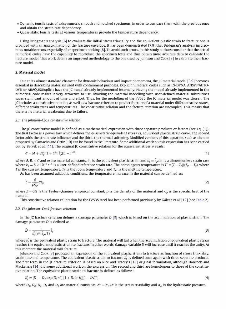
The initial triaxility obtained with Bridgman's formulation (see Eq. (5)), as well as the equivalent plastic strain to fracture obtained after the tests (see Eq. (6)), are summarised in Table 3. The fracture cross section area was perfectly circular as ex­pected (see Fig. 3). Some studies have encountered [4] non-circular fracture areas due to material anisotropy. Hence, there was no need to measure the entire fracture area. The fracture area diameter was enough to obtain proper values of equiv­alent strain to fracture. Note that specimens of Fig. 3 corresponded to the dynamic tests. Nevertheless, the same behaviour was observed for the specimens tested in quasi-static regime. The diameters corresponding to initial and fracture situations were measured with an optical profilometer.

The stress increase in notched specimens came as a consequence of the superimposed circumferential stress state created by the notches (see Fig. 2). In the tensile tests, lower notch radius of the specimens was, larger the increases of the stress were registered. On the other hand, the strain to failure decreased remarkably with the decrease of the notch radius. This showed what has been stated previously; that is to say, the dependency of stress triaxiality on the continuum fracture cri­teria, regardless of whether they are micro- [15] or macro-mechanical [16,17] based models. The accumulation of plastic strain until the specimens fracture was clearly geometry-dependent as can be seen in Fig. 3. In summary, it was noted that the amount of plastic strain necessary to fracture a notched specimen decreased when a smaller notch radius is machined.

Table 1 Certificated chemical composition in %wt of FV535 stainless steel.

C Si Mn S Cr Mo H B Co N Nb V

0.094 0.38 0.77 0.0015 10.28 0.7 0.39 0.007 5.68 0.012 0.31 0.21

Table 2 Johnson-Cook material model constants for FV535, according to [12] and the proposed fracture criterion calibration.

Density (Kg/m Elastic modulus (GPa) Poisson's ratio Specific Heat Q/KgK) Tm (°C)

7850 A (MPa) 1035 Di 0.1133

210 B(MPa 190 D2

2.11

0.28 n 0.3 D3

-1.65

460 C 0.006 D4

0.0125

870 m 4.5 D5

0.9768

Table 3 Diameter reduction (dojdf), initial stress triaxiality (Eq. (5)) and equivalent plastic strain to fracture (Eq. (6)) for axisymmetric smooth and notched specimens.

Specimen ID Notch radius (mm) Test regime df (mm) (doldf) Initial triaxiality

SE01 SE02 SE03 SE04

R401 R402 R403 R404

R201 R202 R203 R204

R101 R102 R103 R104

Smooth

4.0

2.0

1.0

Quasi-static Quasi-static Dynamic Dynamic

Quasi-static Quasi-static Dynamic Dynamic

Quasi-static Quasi-static Dynamic Dynamic

Quasi-static Quasi-static Dynamic Dynamic

2.580 2.665 2.517 2.537

3.135 3.240 2.968 2.904

3.290 3.260 3.129 3.269

3.475 3.535 3.671 3.658

1.550 1.501 1.589 1.577

1.276 1.235 1.348 1.377

1.216 1.227 1.278 1.224

1.151 1.132 1.090 1.093

1/3

0.556

0.739

1.026

0.877 0.812 0.926 0.911

0.462 0.484 0.566 0.597

0.391 0.409 0.495 0.441

0.281 0.247 0.172 0.179

2000

R101 R=1 mm R102R=1 mm R201 R=2mm R202 R=2 mm R401 R=4mm R402 R=2 mm SED1 Snrmolh SE02Smoofri

010 0.00 0.02 004 006 0 08 0.10 012 014

Engineering Strain

Fig. 2. Engineering stress-strain curves obtained from quasi-static tensile tests of smooth and notched specimens.

3.3. Dynamic tensile tests. Group II

The testing of axisymmetric smooth and notched specimens was carried out with a tensile Split Hopkinson Pressure Bar (SHPB) at room temperature. The tensile SHPB geometry and configuration used for the dynamic tensile tests is detailed in Fig. 4. The tensile SHPB comprised an input and output bar, both of steel (elastic modulus Eb = 200 GPa and Poisson ra­tio = 0.3). Input bar was 4500 mm in length and the output 1500 mm. The diameter was 22 mm in both cases. The projectile or striker bar was a steel tubular cylinder of 400 mm length. The striker bar was launched with compressed air inside a

1 3 Fig. 3. Fractured smooth and notched axisymmetric specimens after quasi-static tests. R101 (a), R201 (b), R401 (c) and SE02 (d).

jnoi) Him

Projectile

4(1(1 nun

c

1500 mm 1500 mm 750 mm 750 mm

0Aa = 4 mm 0,4j = 19mm

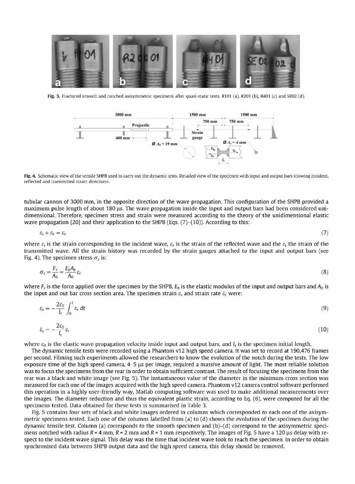
Fig. 4. Schematic view of the tensile SHPB used to carry out the dynamic tests. Detailed view of the specimen with input and output bars showing incident, reflected and transmitted strain directions.

tubular cannon of 3000 mm, in the opposite direction of the wave propagation. This configuration of the SHPB provided a maximum pulse length of about 180 u.s. The wave propagation inside the input and output bars had been considered uni­dimensional. Therefore, specimen stress and strain were measured according to the theory of the unidimensional elastic wave propagation [20] and their application to the SHPB (Eqs. (7)-(10)). According to this:

£,- + £r — £f (7)

where e, is the strain corresponding to the incident wave, er is the strain of the reflected wave and the et the strain of the transmitted wave. All the strain history was recorded by the strain gauges attached to the input and output bars (see Fig. 4). The specimen stress as is:

(8)

where Fs is the force applied over the specimen by the SHPB, Eb is the elastic modulus of the input and output bars andAb is the input and out bar cross section area. The specimen strain es and strain rate ss were:

2co " Is

2C0

srdt

U -Er

(9)

(10)

where c0 is the elastic wave propagation velocity inside input and output bars, and ls is the specimen initial length. The dynamic tensile tests were recorded using a Phantom vl2 high speed camera. It was set to record at 190,476 frames

per second. Filming such experiments allowed the researchers to know the evolution of the notch during the tests. The low exposure time of the high speed camera, 4-5 u.s per image, required a massive amount of light. The most reliable solution was to focus the specimens from the rear in order to obtain sufficient contrast. The result of focusing the specimens from the rear was a black and white image (see Fig. 5). The instantaneous value of the diameter in the minimum cross section was measured for each one of the images acquired with the high speed camera. Phantom vl2 camera control software performed this operation in a highly user-friendly way, Matlab computing software was used to make additional measurements over the images. The diameter reduction and thus the equivalent plastic strain, according to Eq. (6), were computed for all the specimens tested. Data obtained for these tests is summarised in Table 3.

Fig. 5 contains four sets of black and white images ordered in columns which corresponded to each one of the axisym­metric specimens tested. Each one of the columns labelled from (a) to (d) shows the evolution of the specimen during the dynamic tensile test. Column (a) corresponds to the smooth specimen and (b)-(d) correspond to the axisymmetric speci­mens notched with radius R = 4 mm, R = 2 mm and R = 1 mm respectively. The images of Fig. 5 have a 120 |j.s delay with re­spect to the incident wave signal. This delay was the time that incident wave took to reach the specimen. In order to obtain synchronised data between SHPB output data and the high speed camera, this delay should be removed.

^^^B^^H ^^^^H|^| ̂ ^^B^^| I I

(a) (b) (c) (d) Fig. 5. High speed camera photographs for axisymmetric smooth and notched specimens. Fig. shows one representative specimen for each one of the different geometries tested. Specimens' failure at 190 us for SE04 (a), at 95 |is for R404 (b), at 85 |is for R203 (c) and at 35 |is for R103 (d).

As has been pointed out before, when the specimens start necking they change their shape and stop being circular (see column (a) from Fig. 5). Other researchers [21] have addressed the same effects in SHPB tensile tests. Observing Fig. 5, it can be noted that the notch radius changed from its initial "U" shaped form to a "V" shaped form when the specimen was close to fracture. The time in which the fracture occurred diminished quite rapidly with a decreasing notch radius. The smooth specimen fracture occurred at about 185-190 LIS. Fracture for the axisymmetric specimens with notch radius R = 4 mm, R = 2 mm and R = 1 mm occurs at 90-95 LIS, 80-85 LIS and 30-35 LIS respectively (see Figs. 5 and 11). A dynamic test fracture time analysis can give an idea of the complexity when trying to extract valid data from these experiments, especially from the specimens with smallest notch radius.

3.4. Quasi-static tensile tests at various temperatures. Group III

Quasi-static tensile tests of flat specimens with "dog-bone" shape were carried out at room temperature, 200 °C, 400 °C, 500 °C and 600 °C in a universal INSTRON servo hydraulic testing machine. The tests were performed at a strain rate of 5 x 10~4s~\ The flat specimens were tested inside a temperature chamber made "in house". The temperature chamber was equipped with two heat resistant glasses in order to observe the interior of it while the test was ongoing. A thermocou­ple in contact with the specimens was used to control the temperature chamber. In such a way, specimens were set to de­sired temperatures. Note that temperature in the chamber might not have been the same as that of the specimens. A digital camera was used to record images during the tensile tests. In order to measure flat specimen strains, digital image correla­tion software was used. The software provided by correlated solutions used for this purpose was VIC 2D digital image cor­relation software.

Table 4 Area reduction ratio (A0jAf) and equivalent plastic strain to fracture according to Eq. (6) for tests on temperature test specimens.

Specimen identification Temperature (°C) Test regime Af (mm (AolAf)

T01 T02

T05 T08

Til T12

T14 T15

T10 T13

24

200

400

500

600

Quasi-static

Quasi-static

Quasi-static

Quasi-static

Quasi-static

3.707 3.668

3.409 3.404

3.242 3.196

2.609 2.546

1.434 1.527

2.158 2.181

2.347 2.350

2.503 2.468

3.066 3.142

5.580 5.240

0.770 0.780

0.853 0.855

0.918 0.903

1.120 1.145

1.719 1.656

1200

0.10 0.15

Engineering Strain

0.25 100 200 300 400 500

Temperature (°C|

600 700

Fig. 6. (a) Engineering stress-strain curves of quasi-static tests tensile tests carried out at 24 °C, 200 °C, 400 °C, 500 °C and 600 °C. (b) Evolution of the equivalent plastic strain to fracture with increasing temperature including fracture surfaces of specimens tested.

In order to obtain the equivalent plastic strain to fracture of the specimens (see Eq. (6)), measurements of the cross sec­tion fracture areas were taken (see Table 4). Using optical microscopy images of the fracture cross section areas were taken for all the specimens (see Fig. 6b). Specimen fracture cross section areas were measured with image-processing software. The calibration measures needed by the image-processing software were taken with an optical profilometer.

The stress dropped with the temperature increase (see Fig. 6a), especially above 500 °C when it did so significantly. Note that the fracture strain did not vary much until 400 °C. The point when the temperature increased above 400 °C is when sub­stantial changes were noted. When plotting temperature vs. equivalent plastic strain to fracture (Fig. 6b), such behaviour could be observed quite clearly. The first part of the curve presented an almost linear increase on equivalent plastic strain to fracture with the temperature with a small slope. The second part of the curve, exceeding 400 °C, presented a curved shape with a rather marked increase on equivalent plastic strain to fracture with the temperature.

4. Calibration of the Johnson-Cook fracture criterion

Previous works [7,8,22] have established that calibrating the JC fracture criterion by using only the initial stress triaxiality value provided by Bridgman's formulation (Eq. (5)) may involve significant errors. Given that Johnson and Cook [3] and John­son [23] were aware of this, they performed a series of numerical simulations to "correct" such errors. From the point of view of the authors, a more precise calibration could be made. Therefore the subsequent calibration methodology is proposed:

• Compute numerical simulations of the tested specimens with a suitable non-linear finite element code and a proper con­stitutive relation. It should be noted that there is no need to use fracture criterion.

• Obtain the initial stress triaxiality value (just for axisymmetric smooth and notched specimens) (Eq. (5)) and equivalent plastic strain to fracture (Eq. (6)) of the specimens tested (Tables 3 and 4).

• Find the time step in which the minimum cross section diameter (or area) of the finite element model in the numerical simulation has the same value as the fracture diameter (or area) measured in the specimen.

• Obtain, at this time step, stress triaxility and equivalent plastic strain histories in the most critical elements. The authors understand critical elements as those for which the values of stress triaxiality and equivalent plastic strain values are the most unfavourable. It should be noted that for the original JC calibration [3], stress triaxility and equivalent plastic strain histories are averaged over the minimum cross section area.

• Obtain two sets of points in stress triaxility vs. equivalent plastic strain to fracture space. The first set of points includes initial stress triaxility from Bridgman's approach and equivalent plastic strain to fracture obtained from fracture diameter (or area) measurements (Eq. (6)). On the other hand, the second set of points is constructed with the stress triaxiality and equivalent plastic strain to fracture taken from most unfavourable elements of the numerical simulations.

The objective of this calibration methodology is to average two sets of points. One of these sets is the "upper" fracture limit and the other is the "lower". The points belonging to the "upper" fracture limit are the ones calculated with numerical simulations. The reason for choosing the most unfavourable elements for obtaining the stress triaxiality and equivalent plas­tic strain histories, instead of averaging the value of them over the minimum cross section area, is linking a physical meaning to the set of points that authors have designated as "upper" fracture limit. The critical elements in the specimen minimum cross section area should correspond, theoretically to the fracture initiation point, as shown later in the article. The points corresponding to the "lower" fracture limit are those calculated with Bridgman's analysis. This set of points is an approxi­mation to the real fracture behaviour, because of the error committed in assuming initial triaxiality constant (see previous section). This "lower" fracture limit can be considered as conservative, ensuring component safety when designing.

It should be noted that the difference between the original JC fracture criterion calibration [3] and the proposed one is only an "upper" fracture limit set of points. The values of stress triaxiality and equivalent plastic strain are also obtained from the numerical simulations. The difference is that these values are averaged over the minimum cross section area of the finite element model of the specimen.

4.1. Numerical simulations of axisymmetric smooth and notched specimens

Full 3D numerical simulations of quasi-static tensile tests of flat and axisymmetric smooth and notched specimens were carried out with ABAQUS/Standard v6.8 implicit non-linear finite element code. Nine different finite element models were simulated: four corresponding to the axisymmetric smooth and notched specimens; and five corresponding to the different temperatures of the flat specimens. The material was modelled as elastic-plastic with isotropic hardening. The numerical simulations for the specimens tested at room temperature had the same stress-strain curve. For numerical simulations of flat specimens, an additional four different stress-strain curves, one for each temperature, were needed. These curves were obtained from the experiments previously carried out by Galvez et al. [12]. The numerical simulations were performed with only the constitutive relation. No fracture criterion was introduced, the aim of the simulations was not a validation process, but only a calibration.

The meshes of the finite element models used for axisymmetric smooth and notched specimens are shown in Fig. 7. The mesh of the axisymmetric smooth specimen had 115,089 elements. The axisymmetric specimens with notch radius R = 4 mm, R = 2 mm and R = 1 mm, had 109,181, 91,200 and 88,800 elements respectively. All the models were computed with C3D8R eight node linear elements with reduced integration ABAQUS elements, in order to reduce the calculation time.

The numerical simulations for the axisymmetric smooth and notched specimens showed good agreement with the exper­imental force-displacement register, as can be seen in Fig. 8. Nonetheless, the numerical solution for the specimen with the smallest notch radius (R = 1 mm) appeared to be marginally above that expected. In order to obtain the stress triaxiality and equivalent plastic strain to fracture histories from the most critical elements, the minimum cross section area in the fracture time step was analysed. Fig. 9 shows the variation of the stress triaxiality and equivalent plastic strain along the diameters of the minimum cross section areas of axisymmetric smooth and notched specimens. For all the specimens simulated, the stress triaxiality was stronger in the centre of the minimum cross section area, as expected [15]. The equivalent plastic strain showed the same tendency as the stress triaxiality. Nevertheless, the gradient between the borders and the centre of the specimens was not as marked as the stress triaxiality values, especially for the notched specimens. The variation of the equivalent plastic strain along the minimum cross section diameter of smallest notch radius specimen (R = 1 mm) showed an opposite behaviour. The difference between the border and the centre values of the equivalent plastic strain values was

(a) ^ (b) ^ (c) ( d ) ^

Smooth ^ ^ R=4 mm ~ R=2 mm ^ R=1 mm

Fig. 7. 3D finite element model meshes of smooth (a) and notched specimens with notch radius of 4 mm (b), 2 mm (c) and 1 mm (d) for ABAQUS/Standard and LS-DYNA numerical simulations.

10000

5000

.

* • • ,

If \ » R=1mm

3ff *aX R= 2mm

1 Vf

V^. R = 4mm

ABAQUS/Standard Experimental data

^ ^ = V i i ^ - ^ ^

,

Smooth

* » ̂ ~~^~^

0.0 0.5 10 1.5 2.0 Displacement (mm)

Fig. 8. Load-displacement curves from quasi- static tensile tests of smooth and notched axisymmetric specimens compared with ABAQUS/Standard numerical simulations.

1

0.2 0.4 0.6 Normalized diameter

0.2 0.4 0.6 0.8 Normalized diameter

Fig. 9. Stress triaxiality ratio (a) and equivalent plastic strain (b) over the normalised radius of the minimum cross section for smooth and notched axisymmetric specimens obtained from ABAQUS/Standard numerical simulations.

very low, remaining almost constant. Summarising, the critical element (as previously shown) were in the centre of the min­imum cross sections area.

The dynamic tensile tests were simulated with LS-DYNA v971 explicit non-linear finite element code. The same 3D finite element model meshes as those shown in Fig. 7 were used. In order to simulate the tensile SHPB tests of axisymmetric smooth and notched specimens properly, input and output bars were also modelled. The boundary condition was modelled as prescribed velocity in the free end cross section nodes of the input bar with BOUNDARY_PRESCRIBED_MOTION [24]. The incident wave strain can be transformed in velocity according to the unidimensional elastic wave propagation theory as:

V{t)-pC0 m ( i i )

The incident wave signals were recorded from the strain gauges located in the input bar (Fig. 4) for each one of the spec­imens tested. An average value of the incident strain e,(t) was used as boundary condition to compute the numerical simu­lations. The CPU time for these numerical simulations was obviously higher than those computed with ABAQUS/Standard. In order to reduce the calculation time a coarser mesh was used for the input and output bars (Fig. 10). The specimen material

Fig. 10. Finite element model of a tensile SHPB test for LS-DYNA non-linear finite element code. The specimen in the figure is a notched axisymmetric specimen with notch radius equal to 4 mm. Input and output bars are modelled with coarser elements in order to reduce calculation time.

was modelled with MAT_015 [24], JC material model. Only the constants for theJC constitutive relation were introduced (see Table 2), no fracture criterion was used. This material model must be consequent with the quasi-static models simulated in the ABAQUS/Standard.

Good agreement was obtained between the experimental diameter reduction and that from LS-DYNA, as shown in Fig. 11. The same analysis as that carried out for the numerical simulations of the quasi-static tensile tests was performed. The same conclusions emerged: the most critical elements of the minimum cross section area immediately before fracture were lo­cated in its centre. Hence, stress triaxiality and equivalent plastic strain histories were obtained from the elements located in the centre of the minimum cross section area.

The "lower" and "upper" fracture limit sets of points (the first corresponding to the Bridgman's analysis and the second to the numerical simulations of the critical elements), are plotted in the stress triaxiality vs. equivalent plastic strain to fracture

2.0 50 100

Time (us) 150 200 100

Time (u,s) 200

(d)f £ 4.0

40 60

Time (us) 100

3 3 o> E 2 T3

e .2 3.6 •t— o «

3.4

3.2

3.0

Notched R=1mm

LS-DYNA Test R103 Test R104

20 40 60

Time (us)

SO 100

Fig. 11. Minimum cross section diameter reduction from tensile SHPB tests of smooth and notched axisymmetric specimens with notch radius equal to 4 mm, 2 mm and 1 mm, compared with LS-DYNA numerical simulations.

LOW STRAIN RATE Fracture points Bridgmatfs analysis Smooth Bjidgman1? analysis R=4 mm Gldgrran's analysis R=2 mm Bridginan's analysis R-4 mm ABAQUS/Standard Smooth ABAQUS/Standard R-4 mm A BAQU ̂ Standard R=2 mm ABAQUS/Standard R=1 mm

0.3 0.6 0,9 1.2 1.5 Stress triaxiatity

1.8 2.1

0.2

0.0

c k-

tn rt

V, re a.

c QJ re > 3

s

1.6

1.4

1.2

1.0

nf l

Ofi

0.4

HIGH STRAIN RATE

I

Fracture points Brkjgman's analysis Smooth Bridgman's analysis R-£ mm Bridgman's analysis R=2 mm Bridgman's analysis R=l mm LS-DYNA Unnotified LSDYNAR=4mm LE-DYNA R-J mm LS-DYNA R-1 mm

-0.3 0.0 0.3 0.6 0 9 1.2 1.5 Stress triaxiality

(b) 1.S 2.1

Fig. 12. Equivalent plastic strain vs. Stress triaxiality showing fracture points for quasi-static (a) and dynamic (b) cases. Black lines correspond to numerical simulation analysis and dotted lines correspond to Bridgman's analysis.

space in Fig. 12. The point sets corresponding to the quasi-static tensile tests and the sets corresponding to the dynamic ten­sile tests are plotted in Fig. 12a and b respectively. With regard to the quasi-static tensile tests, while the stress triaxiality remains constant in the set of points corresponding to Bridgman's analysis the set of points belonging to the numerical sim­ulations, shows increasing stress triaxiality with the equivalent plastic strain until fracture occurs (see Fig. 12a). This effect is more marked for specimens with larger initial stress triaxialities. The same conclusion can be made for the dynamic case (see Fig. 12b).

4.2. Numerical simulations of flat specimens

The numerical simulations of the flat "dog-bone" shaped specimens were carried out using ABAQUS/Standard non-linear finite element code. The 3D finite element model mesh used has 13,309 elements. The elements used were the same as those in simulating axisymmetric smooth and notched specimens, the C3D8R ABAQUS elements. Five numerical simulations were run, at room temperature, 200 °C, 400 °C, 500 °C and 600 °C. The material was modelled as elastic-plastic with isotropic hardening.

The agreement between experimental and numerical load-displacement (see Fig. 13a) curves was satisfying; neverthe­less, the numerical simulation ran at 600 °C was challenging. The elements were subjected to extremely large strains; thus, the elements suffered significant distortions, which led to some degree of uncertainty. In addition, the experimental results

8000

=• 6000

I 4000

2000

2.0

3 (J ra

4 -O 1.5 c s % £ i.o M

g 0.5

2 3 Displacement (mm)

o.o

(b)

D.= 0 9769

• O

a

• : ;

*

• •

0

ABAQUS/Standard Experimental data

0.2 0.4 0.6 0.8 Homologous temperature (T*)

Fig. 13. (a) Load-displacement curves of flat specimens tested at different temperatures in quasi-static regime compared with ABAQUS/Standard numerical simulations, (b) Evolution of the equivalent plastic strain to fracture with the homologous temperature. Hollow circles correspond to ABAQUS/Standard numerical simulations and black circles to the experimental results.

from quasi-static tensile tests at 600 °C were somewhat imprecise due to the large deformations of the specimens and air diffraction inside the temperature chamber. The authors are aware of the uncertainties that these effect might have caused in the values of the equivalent plastic strain to fracture.

The analysis of the minimum cross section at fracture time step was more complex than that conducted for the axisym-metric specimens. The lack of axial symmetry, due to the rectangular shape of the cross section area, implied that the evo­lution of it would not be uniform. In order to assess the equivalent plastic strain on the minimum cross section area, two imaginary axes were traced: the first one designated as "long axis" and the second one as "short axis" (see Fig. 14). The equivalent plastic strain variation in the short axis was less than in the long one, though the maximum value of both coin­cided at the same position, the centre of the specimen. Hence, it can be concluded that the most critical elements were again in the centre of the specimen.

4.3. JC fracture criterion constant identification

The calibration of the JC fracture criterion implies that five constants must be identified (see Eq. (4)). Such calibration was carried out using the two data sets, Bridgman's analysis ("lower" fracture limit) and values from critical elements of the numerical simulations. Based on the calibration method used by Johnson and Cook [3], an average of the two data series were used for the model calibration (see Table 2).

The first part of the calibration used the results from the axisymmetric smooth and notched specimens, which had pro­vided information of the values of equivalent plastic strain to fracture as function of stress triaxiality and strain rate. Hence, the first four material constants, D^ D2, D3 and D4, were identified in this part of the calibration. D^ D2 and D3 constants belong to the first factor of the Eq. (4), which is triaxiality dependent and D4 belongs to the second factor of Eq. (4), which is strain-rate dependent. All the axisymmetric specimens were tested at room temperature. Temperature dependency of the equivalent plastic strain is then ignored for the time being. Eq. (4) can be rewritten in this case just with the first two factors only:

% = [Dj +D2exp(D3<7*)][l +D4lng;] (12)

Other authors [2,11] have fitted similar expressions minimising the residuals with success. The mathematical expression to minimise is the following:

E E W > J } ~ Pi +D2exp(D3(7*{i})]

where s£{!, j} is a matrix with dimension i x j and a*{i] and sp{j} are J x i and J x j column matrices respectively. The J x i column matrix records the stress triaxiality values and the J x j column records the strain rate values. N, and N,- are the max­imum number of rows and columns of the matrices. The i x j matrix contains the values of the equivalent plastic strain to fracture corresponding to rows of the column matrices of the stress triaxiality and strain rate values.

TRIAXIALITY Eft. PLASTIC STRAIN 0.9 I— — 0.8

— O — Long axis — • — Long axis - - O - - Short axis — • - - S h o r t axis

Nomalized axis distance

Fig. 14. Equivalent plastic strain profile along two perpendicular axes over the minimum cross section. Profiles obtained from ABAQUS/Standard numerical simulations of room temperature quasi-static tensile test of a flat specimen.

-D4lrTp £oJ/} (13)

The second part of the calibration consisted in identifying the last material constant, D5. In this part only the information provided by the quasi-static tensile tests of flat specimens was used. The equivalent plastic strain to fracture of the specimen tested at room temperature [s£]RT was used as a reference. These specimens were conducted at strain rate of 5 x 10~4 s~\ making the second factor equal to the unity. Due to the low strain rate at which the specimens were conducted, adiabatic heating was not taken into account for D5 material constant identification. It should be noted that the adiabatic heating effect was introduced by Johnson and Cook in their original calibration [3], because their specimens were tested in a SHPB, where this effect could be neglected.

The Eq. (4) can be now rewritten as:

e£ = [e£iri+D,r (14)

Plotting equivalent plastic strain to fracture as function of the homologous temperature, a linear fit with D5 as the slope could be made (see Fig. 13b).

5. Conclusions

In this work a combined calibration methodology has been developed for the calibration of the Johnson-Cook fracture criterion. Even though this calibration is based on Johnson and Cook's original paper [3], it includes some novel consider­ations. In order to have a more physically meaningful approach, two data sets were defined:

• The first one is the data set designated as "lower" fracture limit. This data set considers initial triaxiality calculated with Bridgman's analysis (Eq. (5)), as constant. This hypothesis leads to a more "conservative" fracture criterion (see Fig. 15). The final (or fracture) values of minimum cross section diameter (or area) gave the equivalent plastic strain to fracture (Eq. (6)).

• The second is the data set designated as "upper" fracture limit. Stress triaxility and equivalent plastic strain values were obtained from numerical simulations. Original JC fracture criterion's calibration averages these values over the entire minimum cross section area of the specimens. With the new approach proposed, the authors sought to relate the numer­ical simulations with the crack initiation process. In order to obtain the stress triaxialty and the equivalent plastic strain histories that would correspond to the theoretical fracture initiation point, a careful analysis of the minimum cross sec­tion area was performed. The most critical elements, located in the centre of the minimum cross section area, were selected and post-processed.

The material constant identification was made by averaging the two data sets. Nevertheless, the authors have considered that also calibratingJC fracture criterion for the "lower" limit data set and "upper" limit data set (see Table 5) could be useful for the reader.

LU 1

Bridgman's analysis "lower" limit

l l

-0.3 0.0 0 3 06 0.9 Stress triaxiality

1.2 1.5

Fig. 15. Equivalent plastic strain to fracture as function of stress triaxiality.

Table 5 JC fracture criterion calibrations for Bridgman's analysis and numerical simulations.

_Di Eh D3 Di D5

Bridgman ("lower" limit) 0.0005 1.57 -1.93 0.0064 1.1663

Numerical simulations ("upper" limit) 0.0000 3.90 -1.80 0.0070 0.6684

The calibration methodology proposed was applied for the specific case of the FV535 stainless steel. Some difficulties were encountered to perform correct recordings of strain when testing at 600 °C. The authors are aware of the possible errors that might have been committed in the calibration process. The dispersion of the results can be determinant when matching the simulations with the experiments. More careful measurements must be taken in the future for similar experimental pro­cedures. It is intention of the authors to apply the similar calibration methods for different kinds of materials involved in containment tests.

For the case of the FV535 stainless steel the equivalent plastic strain to fracture is not linear with the temperature. The material conserves the linearity until 400 °C, according to that established by Johnson and Cook [3]. However, after exceed­ing this temperature the evolution of the equivalent plastic strain to fracture with the temperature stops being linear. Some correction should be included in the future for JC fracture criterion to include such a type of behaviour.

This work shows the extensive experimental process necessary to perform the calibration of the JC fracture criterion. In order to improve the calibration methodology of this type of fracture criteria, a deep finite element method analysis was per­formed. Relating the numerical simulation top a physical process like fracture initiation offers a better understanding of the problem. The final objective of this study is to check the validity of this calibration methodology. To do so, the authors are at the present carrying out ballistic impact tests, which are a good indicator of the correct behaviour of the model.

It must be pointed out that only tensile tests have been used for the JC fracture criterion calibration. Previous studies [16,25] have shown that the plastic flow and fracture behaviour of ductile materials may b e J 3 (the third invariant of the deviatoric stress tensor) dependent. In other words, the behaviour of the materials might not be the same in tension, com­pression or shear. Such behaviour has not been addressed in the presenting case of the material here, though it is taking into account in the current research carried out by the authors [26].

Acknowledgements

The authors would like to acknowledge the financial support through projects CONSOLIDER INGENIO 2010. The authors would also like to thank the financial support of the Spanish Ministry of Science and Innovation through project with refer­ence BIA2008-06705-C02-01.

References

12 13

14

15

16 17 18 19

[10 111

[12

[13 [14

[15 [16 117 [18

[19 [20

Borvik T, Clausen AH, Eriksson M, Berstad T, Hopperstad OS, Langseth M. Experimental and numerical study on the perforation of AA6005-T6 panels. Int J Impact Eng 2005;32:35-64. Teng X, Wierzbicki T. Evaluation of six fracture models in high velocity perforation. Engng Fract Mech 2006;73:1653-78. Johnson GR, Cook WH. Fracture characteristics of three metals subjected to various strains, strain rates, temperatures and pressures. Engng Fract Mech 1985;21:31-48. Clausen AH, Borvik T, Hopperstad OS, Benallal A. Flow and fracture characteristics of aluminium alloy AA5083-H116 as function of strain rate, temperature and triaxiality. Mater Sci Eng 2004;A364:260-72. Borvik T, Hopperstad OS, Dey S, Pizzinato EV, Langseth M, Albertini C. Strength and ductility of Weldox 460 E steel at high strain rates, elevated temperatures and various stress triaxilities. Engng Fract Mech 2005;72:1071-87. Bridgman PW. Studies in large flow and fracture. New York: McGraw-Hill; 1952. Alves M, Jones N. Influence of hydrostatic stress on failure of axisymmetric notched specimens. J Mech Phys Solids 1999:643-67. Valiente A. On Bridgman's stress solution for a tensile neck applied to axisymmetrical blunt notched tension bars. J Appl Mech 2001;68:412-9. Johnson GR, Cook WH. A constitutive model and data for metals subjected to large strains, high strain rates and high temperatures. In: 7th International symposium on ballistics. The Hague; 1983. p. 541-7. Camacho GT, Ortiz M. Adaptive lagrangian modelling of ballistic penetration of metallic targets. Comput Methods Appl Mech Eng 1997;142:269-301. Borvik T, Hopperstad OS, Berstad T, Langseth M. A computational model of viscoplasticity and ductile damage for impact and penetration. Eur J Mech A Solids 2001;20:685-712. Galvez F, Cendon DA, Enfedaque A, Sanchez-Galvez V. High strain rate and high temperature behaviour of metallic materials for jet engine turbine containment. J Phys IV 2006;134:269-74. Rice JR Tracey DM. On the ductile enlargement of voids in triaxial stress fields. J Mech Phys Solids 1969;17:201-17. Hancock JW, Mackenzie AC. On the mechanisms of ductile failure in high strength steels subjected to multi-axial stress-states. J Mech Phys Solids 1976;24:147-69. Becker R, Needleman A, Richmond O, Tvergaard V. Void growth and failure in notched bars. J Mech Phys Solids 1988;36:317-51. Xue L, Wierzbicki T. Ductile fracture initiation and propagation modeling using damage plasticity theory. Engng Fract Mech 2008;75:3276-93. Bai Y, Wierzbicki T. A new model of plasticity and fracture with pressure and lode dependence. Int J Plast 2008;24:1071-96. Mirone G. Elastoplastic characterization and damage predictions under evolving local triaxility: axysimmetric and thick plate specimens. Mech Mater 2008:685-94. Mirone G, Corallo D. A local viewpoint for evaluating the influence of stress triaxiality and lode angle on ductile failure and hardening. Int J Plast 2009. Kolsky H. Stress waves in solids. New York: Dover Publications; 1963.

[21 ] Hopperstad OS, Borvik T, Langseth M, Labibes K, Albertini C. On the influence of stress triaxiality and strain rate on the behaviour of a structural steel. Part I. Experiments. Eur J Mech A Solids 2003;22:1-13.

[22] Borvik T, Hopperstad OS, Berstad T. On the influence of stress triaxiality and strain rate on the behaviour of a structural steel. Part II. Numerical simulations. Eur J Mech A Solids 2003;22:15-32.

[23] Johnson GR. Tactical missile warheads. Washington, DC: American Institute of Aeronautics and Astronautics; 1993. [24] LS-DYNA KEYWORD USER'S MANUAL Version 971, Livermore Software Technology Corporation, Livermore, California; 2007. [25] Wilkins ML, Streit RD, Reaugh JE. Cumulative-strain-damage model of ductile fracture: simulation and prediction of engineering fracture

tests. Livermore, California: Lawrence Livermore National Laboratory; 1980. [26] Chocron S, Erice B, Anderson CE. A new plasticity and failure model for ballistic application. Int J Impact Eng 2011;38:755-64.