Flow and Congestion Control

2014

Marcos Vieira

Flow Control

• Part of TCP specification (even before 1988)

• Goal: not send more data than the receiver can handle

• Sliding window protocol

• Receiver uses window header field to tell sender how much space it has

Flow Control

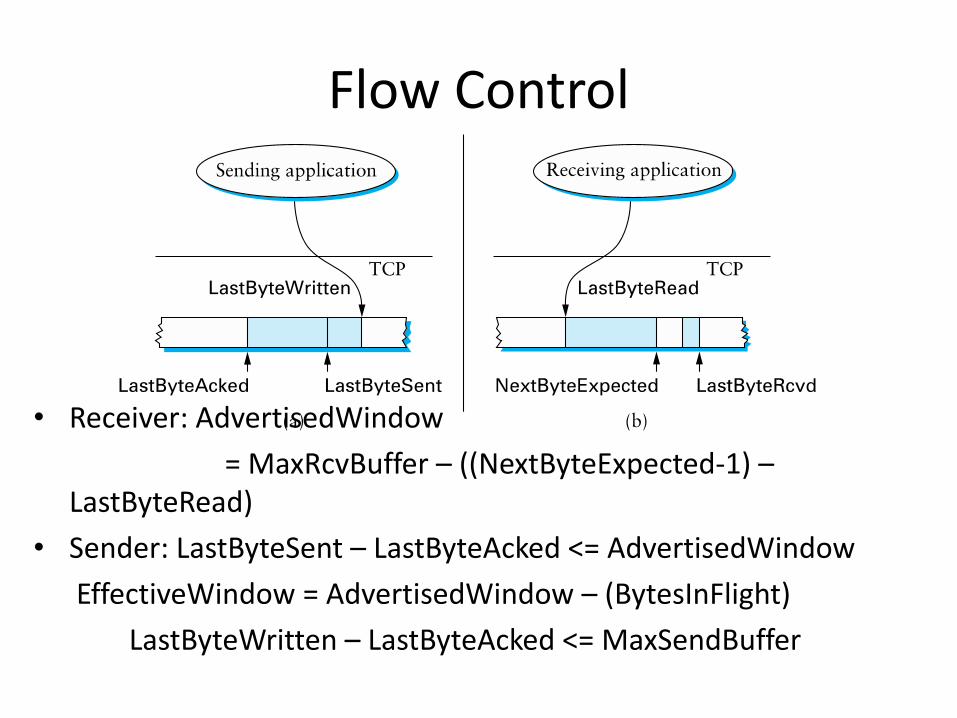
• Receiver: AdvertisedWindow

= MaxRcvBuffer – ((NextByteExpected-1) – LastByteRead)

• Sender: LastByteSent – LastByteAcked <= AdvertisedWindow

EffectiveWindow = AdvertisedWindow – (BytesInFlight)

LastByteWritten – LastByteAcked <= MaxSendBuffer

Delayed Acknowledgments

• Goal: Piggy-back ACKs on data

– Delay ACK for 200ms in case application sends data

– If more data received, immediately ACK second segment

– Note: never delay duplicate ACKs (if missing a segment)

Limitations of Flow Control

• Network may be the bottleneck

• Signal from receiver not enough!

• Sending too fast will cause queue overflows, heavy packet loss

• Flow control provides correctness

• Need more for performance: congestion control

Congestion Control

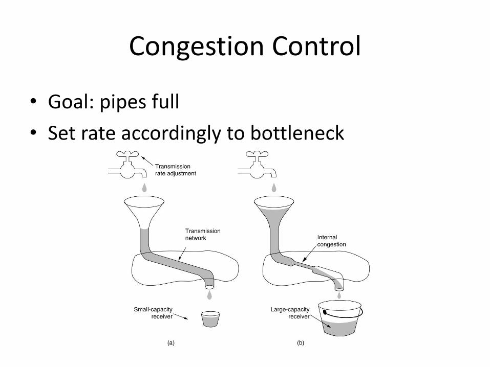
• Goal: pipes full

• Set rate accordingly to bottleneck

Congestion Control

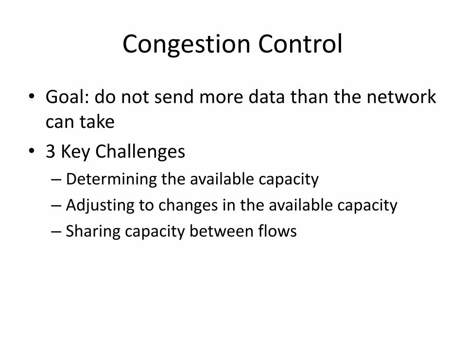
• Goal: do not send more data than the network can take

• 3 Key Challenges

– Determining the available capacity

– Adjusting to changes in the available capacity

– Sharing capacity between flows

TCP Congestion Control

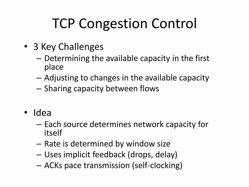
• 3 Key Challenges – Determining the available capacity in the first

place – Adjusting to changes in the available capacity – Sharing capacity between flows

• Idea

– Each source determines network capacity for itself

– Rate is determined by window size – Uses implicit feedback (drops, delay) – ACKs pace transmission (self-clocking)

Dealing with Congestion

• TCP keeps congestion and flow control windows

– Transmit minimum of the two controls

• Sending rate: ~Window/RTT

• The key here is how to set the congestion window to respond to congestion signals

Starting Up

• Before TCP Tahoe

– On connection, nodes send full (rcv)window of packets

– Retransmit packet immediately after its timer expires

• Result: window-sized bursts of packets in network

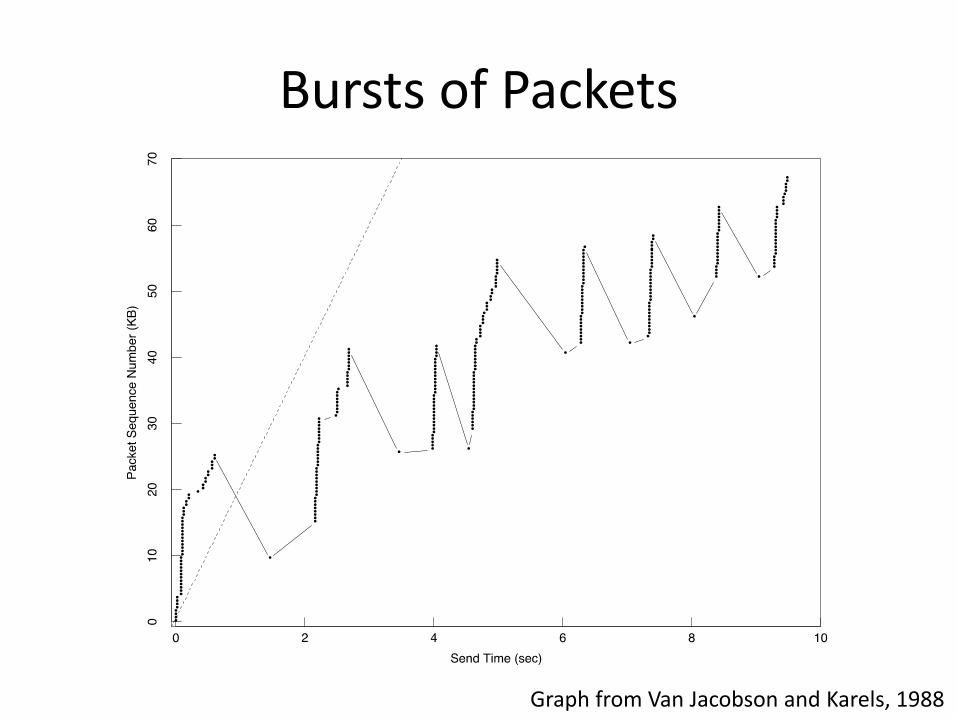
Bursts of Packets

Graph from Van Jacobson and Karels, 1988

Determining Initial Capacity

• Question: how do we set w initially?

– Should start at 1MSS (to avoid overloading the network)

– Could increase additively until we hit congestion

– May be too slow on fast network

• Start by doubling w each RTT

– Then will dump at most one extra window into network

– This is called slow start

• Slow start, this sounds quite fast!

– In contrast to initial algorithm: sender would dump entire flow control window at once

Startup behavior with Slow Start

Slow Start

From [Jacobson88]

Slow start implementation

• Let w be the size of the window in bytes – We have w/MSS segments per RTT

• We are doubling w after each RTT – We receive w/MSS ACKs each RTT

– So we can set w = w + MSS on every ack

• At some point we hit the network limit. – Experience loss

– We are at most one window size above the limit

– Remember this: ssthresh and reduce window

Chronology of a Slow-start

Slow Start

• We double cwnd every round trip

• We are still sending min (cwnd,rcvwnd) pkts

• Continue until ssthresh estimate or pkt drop

http://en.wikipedia.org/wiki/Slow-start

Sender Receiver

pkt

ack

Congestion Collapse

From [Chiu89]

Dealing with Congestion

• Assume losses are due to congestion

• After a loss, reduce congestion window

– How much to reduce?

• Idea: conservation of packets at equilibrium

– Want to keep roughly the same number of packets network

– Analogy with water in fixed-size pipe

– Put new packet into network when one exits

Self-clocking

• So, if packets after the first burst are sent only in response to an ack, the sender’s packet spacing will exactly match the packet time on the slowest link in the path.

Congestion Signal

• If packet loss is (almost) due to congestion, we have a good candidate for the ‘networked is congested’ signal.

• Is it valid?

How much to reduce window?

• What happens under congestion?

– Exponential increase in congestion

• Sources must decrease offered rate exponentially

– i.e, multiplicative decrease in window size

– TCP chooses to cut window in half

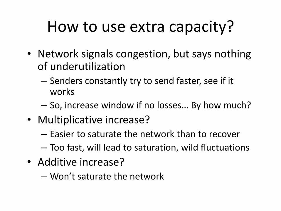
How to use extra capacity?

• Network signals congestion, but says nothing of underutilization – Senders constantly try to send faster, see if it

works

– So, increase window if no losses… By how much?

• Multiplicative increase? – Easier to saturate the network than to recover

– Too fast, will lead to saturation, wild fluctuations

• Additive increase? – Won’t saturate the network

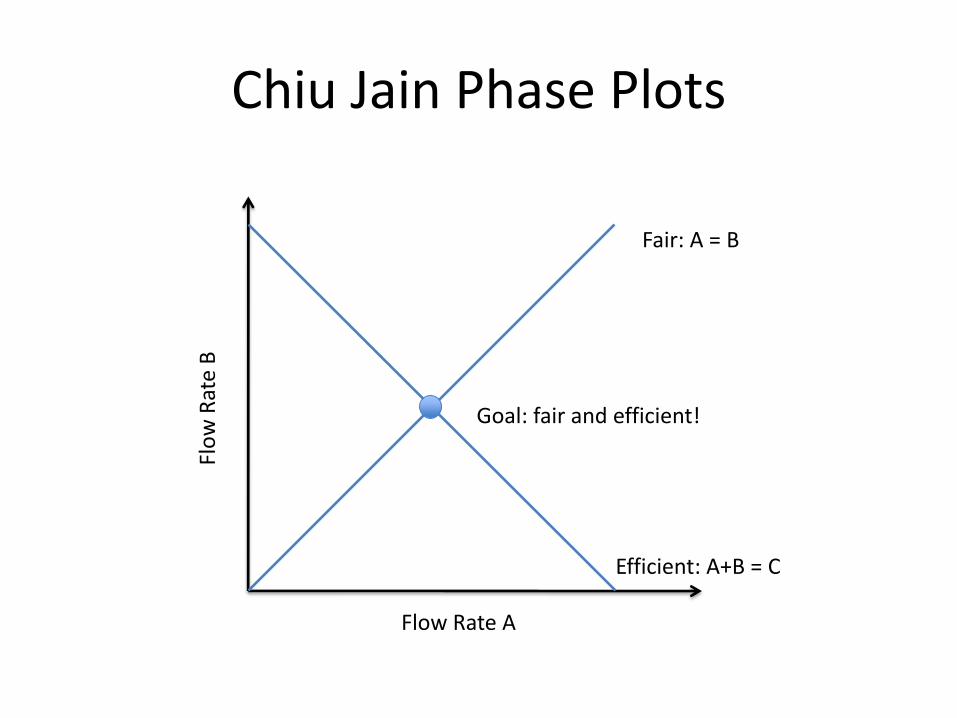
Chiu Jain Phase Plots

Flow Rate A

Flo

w R

ate

B

Fair: A = B

Efficient: A+B = C

Goal: fair and efficient!

Chiu Jain Phase Plots

Flow Rate A

Flo

w R

ate

B

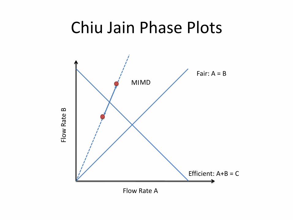
Fair: A = B

Efficient: A+B = C

MD MI

Chiu Jain Phase Plots

Flow Rate A

Flo

w R

ate

B

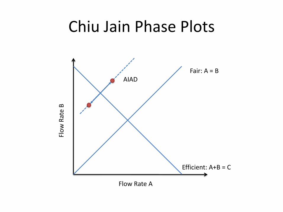
Fair: A = B

Efficient: A+B = C

AD AI

Chiu Jain Phase Plots

Flow Rate A

Flo

w R

ate

B

Fair: A = B

Efficient: A+B = C

AI MD

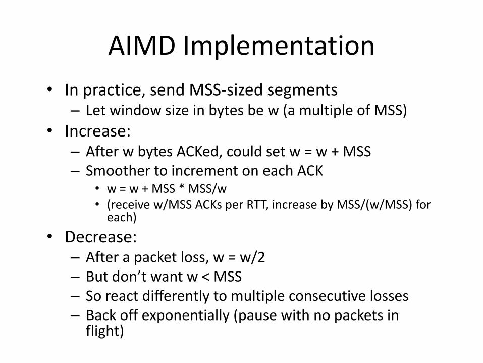
AIMD Implementation

• In practice, send MSS-sized segments – Let window size in bytes be w (a multiple of MSS)

• Increase: – After w bytes ACKed, could set w = w + MSS – Smoother to increment on each ACK

• w = w + MSS * MSS/w • (receive w/MSS ACKs per RTT, increase by MSS/(w/MSS) for

each)

• Decrease: – After a packet loss, w = w/2 – But don’t want w < MSS – So react differently to multiple consecutive losses – Back off exponentially (pause with no packets in

flight)

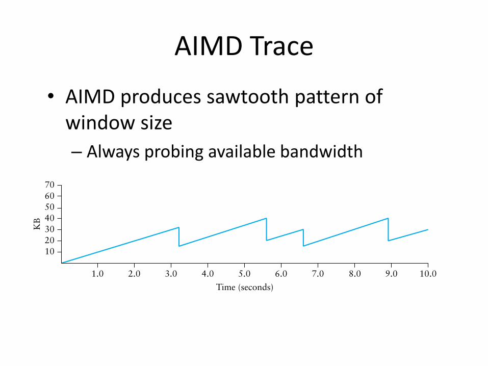
AIMD Trace

• AIMD produces sawtooth pattern of window size

– Always probing available bandwidth

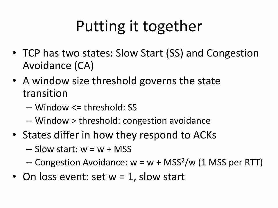
Putting it together

• TCP has two states: Slow Start (SS) and Congestion Avoidance (CA)

• A window size threshold governs the state transition – Window <= threshold: SS

– Window > threshold: congestion avoidance

• States differ in how they respond to ACKs – Slow start: w = w + MSS

– Congestion Avoidance: w = w + MSS2/w (1 MSS per RTT)

• On loss event: set w = 1, slow start

How to Detect Loss

• Timeout

• Any other way?

– Gap in sequence numbers at receiver

– Receiver uses cumulative ACKs: drops => duplicate ACKs

• 3 Duplicate ACKs considered loss

Putting it all together

Time

cwnd

Timeout

Slow Start

AIMD

ssthresh

Timeout

Slow Start

Slow Start

AIMD

RTT

• We want an estimate of RTT so we can know a packet was likely lost, and not just delayed

• Key for correct operation • Challenge: RTT can be highly variable

– Both at long and short time scales!

• Both average and variance increase a lot with load • Solution

– Use exponentially weighted moving average (EWMA) – Estimate deviation as well as expected value – Assume packet is lost when time is well beyond

reasonable deviation

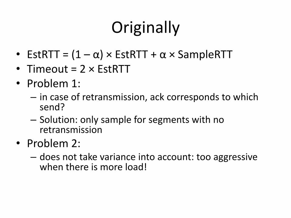
Originally

• EstRTT = (1 – α) × EstRTT + α × SampleRTT • Timeout = 2 × EstRTT • Problem 1:

– in case of retransmission, ack corresponds to which send?

– Solution: only sample for segments with no retransmission

• Problem 2: – does not take variance into account: too aggressive

when there is more load!

Jacobson/Karels Algorithm (Tahoe)

• EstRTT = (1 – α) × EstRTT + α × SampleRTT

– Recommended α is 0.125

• DevRTT = (1 – β) × DevRTT + β | SampleRTT – EstRTT |

– Recommended β is 0.25

• Timeout = EstRTT + 4 DevRTT

• For successive retransmissions: use exponential backoff

Old RTT Estimation 2 CONSERVATION AT EQUILIBRIUM: ROUND-TRIP TIMING 7

Figure 5: Performance of an RFC793 retransmit timer

•

• • • •

••

• •

• •

• •

••• •

••

••

•• • • •

•

•••

•• • • •

• ••

••

• • •• • •

••

• ••

•••

•

• ••

•

••

•

•

••

•

•

• • •

••••

•

•

• •

•

• •

•

• •

••

••

• • •

• ••

•

•

••

•

• •

Packet

RT

T (

se

c.)

0 10 20 30 40 50 60 70 80 90 100 110

02

46

81

01

2

Trace data showing per-packet round trip time on a well-behaved Arpanet connection. The

x-axis is the packet number (packets were numbered sequentially, starting with one) and

the y-axis is the elapsed time from the send of the packet to the sender’s receipt of its ack.

During this portion of the trace, no packets were dropped or retransmitted.

The packets are indicated by a dot. A dashed line connects them to make the sequence eas-

ier to follow. The solid line shows the behavior of a retransmit timer computed according

to the rules of RFC793.

The parameter ! accounts for RTT variation (see [5], section 5). The suggested ! = 2

can adapt to loads of at most 30%. Above this point, a connection will respond to load

increases by retransmitting packets that have only been delayed in transit. This forces the

network to do useless work, wasting bandwidth on duplicates of packets that will eventually

be delivered, at a time when it’s known to be having trouble with useful work. I.e., this is

the network equivalent of pouring gasoline on a fire.

We developed a cheap method for estimating variation (see appendix A)3 and the re-

sulting retransmit timer essentially eliminates spurious retransmissions. A pleasant side

effect of estimating ! rather than using a fixed value is that low load as well as high load

performance improves, particularly over high delay paths such as satellite links (figures 5

and 6).

Another timer mistake is in the backoff after a retransmit: If a packet has to be retrans-

mitted more than once, how should the retransmits be spaced? For a transport endpoint

embedded in a network of unknown topology and with an unknown, unknowable and con-

stantly changing population of competing conversations, only one scheme has any hope

of working—exponential backoff—but a proof of this is beyond the scope of this paper.4

3We are far from the first to recognize that transport needs to estimate both mean and variation. See, for

example, [6]. But we do think our estimator is simpler than most.4See [8]. Several authors have shown that backoffs ‘slower’ than exponential are stable given finite popula-

tions and knowledge of the global traffic. However, [17] shows that nothing slower than exponential behavior

will work in the general case. To feed your intuition, consider that an IP gateway has essentially the same

behavior as the ‘ether’ in an ALOHA net or Ethernet. Justifying exponential retransmit backoff is the same as

Tahoe RTT Estimation

3 ADAPTING TO THE PATH: CONGESTION AVOIDANCE 8

Figure 6: Performance of a Mean+Variance retransmit timer

•

• • • •

••

• •

• •

• •

•

•• •

••

••

•• • • •

•

•••

•• • • •

• ••

••

• • •• • •

••

• ••

•••

•

• ••

•

••

•

•

••

•

•

• • •

••••

•

•

• •

•

• •

•

• •

••

••

• • •

• ••

•

•

••

•

• •

Packet

RT

T (

sec.)

0 10 20 30 40 50 60 70 80 90 100 110

02

46

81

01

2

Same data as above but the solid line shows a retransmit timer computed according to the

algorithm in appendix A.

To finesse a proof, note that a network is, to a very good approximation, a linear system.

That is, it is composed of elements that behave like linear operators — integrators, delays,

gain stages, etc. Linear system theory says that if a system is stable, the stability is expo-

nential. This suggests that an unstable system (a network subject to random load shocks

and prone to congestive collapse5) can be stabilized by adding some exponential damping

(exponential timer backoff) to its primary excitation (senders, traffic sources).

3 Adapting to the path: congestion avoidance

If the timers are in good shape, it is possible to state with some confidence that a timeout in-

dicates a lost packet and not a broken timer. At this point, something can be done about (3).

Packets get lost for two reasons: they are damaged in transit, or the network is congested

and somewhere on the path there was insufficient buffer capacity. On most network paths,

loss due to damage is rare ( 1%) so it is probable that a packet loss is due to congestion in

the network.6

showing that no collision backoff slower than an exponential will guarantee stability on an Ethernet. Unfortu-

nately, with an infinite user population even exponential backoff won’t guarantee stability (although it ‘almost’

does—see [1]). Fortunately, we don’t (yet) have to deal with an infinite user population.5The phrase congestion collapse (describing a positive feedback instability due to poor retransmit timers) is

again the coinage of John Nagle, this time from [23].6Because a packet loss empties the window, the throughput of any window flow control protocol is quite

sensitive to damage loss. For an RFC793 standard TCP running with window w (where w is at most the

bandwidth-delay product), a loss probability of p degrades throughput by a factor of (1 + 2pw)− 1. E.g., a 1%

damage loss rate on an Arpanet path (8 packet window) degrades TCP throughput by 14%.

The congestion control scheme we propose is insensitive to damage loss until the loss rate is on the order of

the window equilibration length (the number of packets it takes the window to regain its original size after a

loss). If the pre-loss size is w, equilibration takes roughly w2/ 3 packets so, for the Arpanet, the loss sensitivity

Slow start every time?

• Losses have large effect on throughput

• Fast Recovery (TCP Reno)

– Same as TCP Tahoe on Timeout: w = 1, slow start

– On triple duplicate ACKs: w = w/2

– Retransmit missing segment (fast retransmit)

– Stay in Congestion Avoidance mode

Transport Layer 3-39

X

Figure 3.37 Resending a segment after triple duplicate ACK

D1 D2 D3 D4 D5 A1

A1 A1 A1

Fast Recovery and Fast Retransmit

Time

cwnd

Slow Start

AI/MD

Fast retransmit

3 Challenges Revisited

• Determining the available capacity in the first place – Exponential increase in congestion window

• Adjusting to changes in the available capacity – Slow probing, AIMD

• Sharing capacity between flows – AIMD

• Detecting Congestion – Timeout based on RTT – Triple duplicate acknowledgments

• Fast retransmit/Fast recovery – Reduces slow starts, timeouts