University of Reading School of Mathematics, Meteorology & Physics

Flood Prediction and Uncertainty

by

Evangelia-Maria Giannakopoulou August 18, 2008

--------------------------------------------------------------------------------

This dissertation is submitted to the Department of Mathematics and Meteorology in partial fulfilment of the requirements for the degree of Master of Science

Abstract A grid-based approach to fluvial flood modelling has been investigated in this

dissertation. A spatially-distributed hydrological model can simulate flow on an area-

wide basis and a runoff production is used to estimate river flows with a simple kinematic

wave scheme. Initialization errors, (rainfall) input errors and forecast model errors are the

main sources of uncertainty in flood modelling. Since, there is uncertainty associated

with rainfall inputs whatever the resolution of the flood forecasting model, an approach

has been developed that uses an ensemble forecasts of rainfall as an input to an ensemble

flood model. It seems natural to combine this approach with an ensemble data

assimilation system. The Ensemble Kalman Filter (EnKF) is a data assimilation method

may be used to solve the initialization problem in flood forecasting. The key idea of the

EnKF algorithm is to use a statistical sample of forecasts to calculate a state estimate and

an error covariance matrix that measures the uncertainty in the estimate.

Two main methods used in this dissertation. We developed a simplified one-

dimensional (1-D) distributed flow model and implemented an Ensemble Transform

Kalman Filter (ETKF) for use with rainfall inputs and the simple flood model, as an

illustration of the initialization problem in flood forecasting. We carried out numerical

experiments where we used one forecast of the model as a reference or ‘truth’ trajectory.

Experiments with the simplified 1-D distributed flood model show that low order

numerical schemes tend to have numerical diffusion. Experimental results with the ETKF

are presented also to show that the usage of the simple flood model and the sequential

nature of the ETKF may lead to filter convergence. The ETKF estimates converge to the

true state as the ensemble size increases and if more (imperfect) observations are

assimilated over time. Description of the problems that were encountered in

implementing these two methods and justification of the solutions that were adopted are

given in detail in this dissertation.

ii

Contents List of Symbols vii

List of Abbreviations x

1. Introduction 1

1.1 Background . . . . . . . . . . . . . . . . . . . . . . . . . . . . . . . . . 1

1.2 Goals . . . . . . . . . . . . . . . . . . . . . . . . . . . . . . . . . . . . . 2

1.3 Principal Results . . . . . . . . . . . . . . . . . . . . . . . . . . . . . . . 3

1.4 Outline . . . . . . . . . . . . . . . . . . . . . . . . . . . . . . . . . . . 3

2. Flood Forecasting 5

2.1 Flood Forecasting Models . . . . . . . . . . . . . . . . . . . . . . . . . 5

2.2 Grid-to-Grid Model . . . . . . . . . . . . . . . . . . . . . . . . . . . . . 7

2.2.1 Runoff Model . . . . . . . . . . . . . . . . . . . . . . . . . . . . . 9

2.2.2 Maximum Water Storage Capacity . . . . . . . . . . . . . . . . . . 10

2.2.3 Grid-to-Grid Flow Routing . . . . . . . . . . . . . . . . . . . . . 11

2.2.4 Parameterization . . . . . . . . . . . . . . . . . . . . . . . . . . . 13

2.3 Sources of Uncertainty in Flood Forecasting . . . . . . . . . . . . . . . . 14

2.3.1 Input Uncertainty of Rainfall . . . . . . . . . . . . . . . . . . . . . 15

2.3.2 Model Uncertainty . . . . . . . . . . . . . . . . . . . . . . . . . . 17

2.3.3 Output Uncertainty . . . . . . . . . . . . . . . . . . . . . . . . . . 17

2.4 Case study: The Boscastle Flood . . . . . . . . . . . . . . . . . . . . . 18

2.5 Summary . . . . . . . . . . . . . . . . . . . . . . . . . . . . . . . . . . 21

3. Ensemble Flood Forecasting 22

3.1 Rainfall Inputs . . . . . . . . . . . . . . . . . . . . . . . . . . . . . . . 22

3.2 Model Initialization . . . . . . . . . . . . . . . . . . . . . . . . . . . . . 23

3.3 The Kalman Filter . . . . . . . . . . . . . . . . . . . . . . . . . . . . . 24

iii

3.3.1 The Kalman Filter Algorithm . . . . . . . . . . . . . . . . . . . . . 25

3.4 The Ensemble Kalman Filter . . . . . . . . . . . . . . . . . . . . . . . . 28

3.4.1 Notation . . . . . . . . . . . . . . . . . . . . . . . . . . . . . . . 30

3.4.2 The Forecast Step . . . . . . . . . . . . . . . . . . . . . . . . . . 31

3.4.3 The Analysis Step . . . . . . . . . . . . . . . . . . . . . . . . . . 32

3.5 The Ensemble Square Root Filter . . . . . . . . . . . . . . . . . . . . . 33

3.6 The Ensemble Transform Kalman Filter . . . . . . . . . . . . . . . . . . 34

3.7 Summary . . . . . . . . . . . . . . . . . . . . . . . . . . . . . . . . . . 36

4. A Simplified 1-D Distributed Flow Model 37

4.1 Simplified Distributed Flow Routing . . . . . . . . . . . . . . . . . . . 37

4.2 Analytic Solution . . . . . . . . . . . . . . . . . . . . . . . . . . . . . 39

4.3 Numerical Implementation . . . . . . . . . . . . . . . . . . . . . . . . . 43

4.4 Accuracy of the finite difference scheme . . . . . . . . . . . . . . . . . 44

4.5 Stability of the finite difference scheme . . . . . . . . . . . . . . . . . 46

4.6 Validation of the numerical implementation . . . . . . . . . . . . . . . . 48

4.6.1 Qualitative behaviour of the flow model . . . . . . . . . . . . . . . 49

4.6.2 Validation of the flow model . . . . . . . . . . . . . . . . . . . . . 53

4.7 Summary . . . . . . . . . . . . . . . . . . . . . . . . . . . . . . . . . . 55

5. Implementing an Ensemble Kalman Filter 56

5.1 Implementing the ETKF . . . . . . . . . . . . . . . . . . . . . . . . . . 56

5.2 Implementing the ETKF for use with inputs . . . . . . . . . . . . . . . . 58

5.3 Summary . . . . . . . . . . . . . . . . . . . . . . . . . . . . . . . . . . 61

6. Experimental Results 62

6.1 Experiments with the ETKF . . . . . . . . . . . . . . . . . . . . . . . . 62

6.2 Summary . . . . . . . . . . . . . . . . . . . . . . . . . . . . . . . . . . 72

iv

7. Conclusions 74

7.1 Summary and Discussion . . . . . . . . . . . . . . . . . . . . . . . . . . 74

7.2 Further Work . . . . . . . . . . . . . . . . . . . . . . . . . . . . . . . . 77

A Graphs of the simplified 1-D distributed flow model 78

B Graphs of the ETKF 80

Bibliography 84

Acknowledgements 89

Declaration 89

v

List of Figures 2.1 Framework for a Grid-to-Grid flood model . . . . . . . . . . . . . . . . . 8

2.2 Diagram for runoff production . . . . . . . . . . . . . . . . . . . . . . . . . 9

2.3 Schematic of the Grid-to-Grid model structure . . . . . . . . . . . . . . . . . 12

2.4 Error framework for rainfall-runoff models . . . . . . . . . . . . . . . . . 15

2.5 Rainfall accumulations from 12, 4 and 1-km grid-space forecast models . . . . 19

3.1 Schematic diagram of an EnKF . . . . . . . . . . . . . . . . . . . . . . . . . 29

4.1 Precipitation and Evaporation evolution over the hours of day . . . . . . . . . 40

4.2 Qualitative behaviour of the flow model with time for 05.0=a . . . . . . . . . 51

4.3 Qualitative behaviour of the flow model in space for 05.0=a . . . . . . . . . 52

4.4 Logarithmic rms errors against logarithmic t∆ and x∆ . . . . . . . . . . . . . 54

6.1 ETKF, imperfect observations (1, 5, 10 and 20) over time, perfect background,

4=N : Ensemble members . . . . . . . . . . . . . . . . . . . . . . . . . 66

6.2 ETKF, imperfect observations (1, 5, 10 and 20) over time, imperfect background,

4=N : Ensemble members . . . . . . . . . . . . . . . . . . . . . . . . . 67

6.3 ETKF, perfect background, N = 4, 10, 50 and 100: Ensemble members . . . 68

6.4 ETKF, imperfect observations (1, 15 and 50) in space, observed space grid

point, perfect background, 27=N : Ensemble members . . . . . . . . . . . . . 70

6.5 ETKF, imperfect observations (1, 15 and 50) in space, unobserved space grid

point, perfect background, 27=N : Ensemble members . . . . . . . . . . . . . 71

A.1 Qualitative behaviour of the flow model with time for 005.0=a . . . . . . . . 79

A.2 Qualitative behaviour of the flow model in space for 005.0=a . . . . . . . . 79

B.1 ETKF, imperfect observations (1, 5, 10 and 20) over time, perfect background,

vi

27=N : Ensemble members . . . . . . . . . . . . . . . . . . . . . . . . . 81

B.2 ETKF, imperfect observations (1, 5, 10 and 20) over time, imperfect background,

27=N : Ensemble members . . . . . . . . . . . . . . . . . . . . . . . . . 82

B.3 ETKF, imperfect background, N = 4, 10, 50 and 100: Ensemble members . . 83

List of Tables 4.1 Routing model parameters . . . . . . . . . . . . . . . . . . . . . . . . . 38

4.2 Typical values of model, precipitation and evaporation parameters . . . . . 49

vii

List of Symbols Latin a Parameter that depends on topography.

a (Superscript) Analysis value.

b (Subscript) Sub-surface pathways of water movement.

c Kinematic wave speed.

maxc Upper limit of storage capacity.

E Evaporation.

e Model error.

e (Subscript) Ensemble value.

f (Superscript) Forecast value.

g Average topographic gradient.

maxg Upper limit of gradient.

H Nonlinear observation operator.

H Linear observation operator.

I Identity matrix.

i (Subscript) Ensemble member.

K Kalman gain matrix.

k (Subscript) Position in discrete time.

L Length scale.

l Dimension of rainfall input vector.

l (Subscript) Flow over land.

M Nonlinear dynamical model.

M Linear dynamical model.

m Number of nonzero singular values in SVD.

N Ensemble size.

N Matrix that relates the rainfall input u to the state vector x .

viii

n Dimension of state vector.

n (Subscript) Position in discrete space.

P Precipitation.

P State error covariance matrix.

p Dimension of observation vector.

Q Model noise covariance matrix.

q Channel flow. nkq Flow out of the n th space at time k .

R Return flow.

R Observation noise covariance matrix.

r Return flow fraction.

r (Subscript) Flow over river.

S Ensemble version of innovations covariance matrix.

0S Initial depth of water in storage.

maxS Maximum water storage capacity.

T Post-multiplier in deterministic formulations of EnKF.

T Time scale.

t (Superscript) True value (Chapter 3); time (Chapter 4).

kt Discrete times at which observations are available and forecasts

and analyses are required.

U Column-orthogonal matrix.

u Lateral inflow per unit length of river.

u Rainfall input vector.

V Column-orthogonal matrix.

w Frequency of precipitation.

X Ensemble matrix.

x Space.

x State vector.

Y Observation ensemble matrix.

y Observation vector.

ix

z Frequency of evaporation.

Greek

β Magnitude of evaporation.

γ Phase of evaporation.

δ Phase of precipitation.

ε Observation noise vector.

ζ Gaussian random noise for rainfall input.

η Model noise vector.

θ Dimensionless wave speed.

κ Parameter that depends on soil, geology, terrain and land cover.

Λ Diagonal matrix of nonzero eigenvalues.

λ Model parameter.

Σ Matrix of singular values in SVD.

σ Parameter that depends on topography.

x

List of Abbreviations CEH Centre for Ecology and Hydrology

EKF Extended Kalman Filter

EnKF Ensemble Kalman Filter

EnSRF Ensemble Square Root Filter

ETKF Ensemble Transform Kalman Filter

KF Kalman Filter

NWP Numerical Weather Prediction

ODE Ordinary Differential Equation

PDE Partial Differential Equation

PDM Probability Distributed Model

SRF Square Root Filter

SVD Singular Value Decomposition

1

Chapter 1

Introduction

1.1 Background

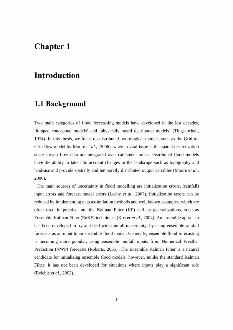
Two main categories of flood forecasting models have developed in the last decades,

‘lumped conceptual models’ and ‘physically based distributed models’ (Tingsanchali,

1974). In this thesis, we focus on distributed hydrological models, such as the Grid-to-

Grid flow model by Moore et al., (2006), where a vital issue is the spatial discretization

since stream flow data are integrated over catchment areas. Distributed flood models

have the ability to take into account changes in the landscape such as topography and

land-use and provide spatially and temporally distributed output variables (Moore et al.,

2006).

The main sources of uncertainty in flood modelling are initialization errors, (rainfall)

input errors and forecast model errors (Leahy et al., 2007). Initialization errors can be

reduced by implementing data assimilation methods and well known examples, which are

often used in practice, are the Kalman Filter (KF) and its generalizations, such as

Ensemble Kalman Filter (EnKF) techniques (Koster et al., 2004). An ensemble approach

has been developed to try and deal with rainfall uncertainty, by using ensemble rainfall

forecasts as an input to an ensemble flood model. Generally, ensemble flood forecasting

is becoming more popular, using ensemble rainfall inputs from Numerical Weather

Prediction (NWP) forecasts (Roberts, 2005). The Ensemble Kalman Filter is a natural

candidate for initializing ensemble flood models, however, unlike the standard Kalman

Filter; it has not been developed for situations where inputs play a significant role

(Reichle et al., 2002).

2

The basic idea of the Ensemble Kalman Filter (EnKF) is to use a statistical sample of

state estimates instead of a single estimate. The mean of this ensemble sample represents

the ‘best’ state estimate, while the variance provides a measure of the spread of the

ensemble errors (Leahy et al., 2007). Also, with the use of a statistical sample in EnKF

algorithm we calculate the error covariance matrix from this ensemble instead of

maintaining a separate covariance matrix and that leads in a better representation of

nonlinearity and is less expensive than the Extended Kalman Filter (Evensen, 2003).

Finally, another benefit of the EnKF comes from the calculation of the Kalman gain

matrix for all statistical members which decreases the fixed cost of the additional

ensemble members (Leahy et al., 2007).

1.2 Goals

The goals of this thesis are

• To design and implement a simplified one dimensional (1-D) distributed flow

model, based on some of the ideas from the distributed Grid-to-Grid model

(Moore et al., 2006 and Bell et al., 2007).

• To implement an Ensemble Square Root Filter (EnSRF), (Livings et al., 2008);

the Ensemble Transform Kalman Filter (ETKF), (Bishop et al., 2001) in

conjunction with this simplified 1-D distributed flow model.

• To modify the ETKF for use with rainfall inputs.

• To investigate the effects of ensemble size and observation frequency on the

behaviour of the forecast - assimilation dynamical system.

3

1.3 Principal Results

A simplified 1-D distributed flow model is selected for implementation in Chapter 4. It is

found to be useful to follow a related to the Grid-to-Grid routing scheme that described in

Chapter 2 and to assume periodic boundary conditions for reasons of simplicity.

Experiments with this simplified 1-D distributed flood model in Chapter 4 (Section 4.6)

show that low order numerical schemes, such as the upwind scheme (first order accurate

in time and space) used to integrate the simple kinematic wave equation (4.1) of the flow

model in Section 4.1, tend to have numerical diffusion.

The Ensemble Transform Kalman Filter (ETKF) using rainfall inputs and the simple

flood model, which described in Chapter 4, is selected for implementation in Chapter 5.

Experiments with the ETKF, in Chapter 6, show that the usage of a simplified low

dimensional distributed flow model and the sequential nature of the ETKF may lead to

filter convergence. In view of the experimental results in Chapter 6, we expect that the

assimilation results might be quite different when obtained on the basis of a more active

assimilation model than the one we use in this research. Such a model will be if we

increase the dimension of the state space, the number of days we run the model and the

size of ensemble members.

1.4 Outline

In Chapter 2 two main points are selected for discussion. Firstly, we present an overview

of flood forecast models, focusing on the Grid-to-Grid flow model (physically based

distributed model), and then consider the application of these models to extreme flood

conditions. The second focus is on sources of uncertainty in flood modelling.

Chapter 3 describes data assimilation methods which are useful in flood forecasting,

since the use of real-time flood models requires attention to uncertainty estimation and

model initialization (i.e. state estimation); problems which can be solved using data

assimilation techniques. In particular, this Chapter presents basic information about

4

ensemble forecasting, data assimilation and describes the techniques of Kalman and

Ensemble Kalman Filters.

In Chapter 4, as a subject for experiments, a simplified 1-D distributed flow model is

introduced. It describes the methodology of the simple flood model and presents some

basic validation results with problems that were encountered and new ideas that used in

the implemented simple flood model.

In Chapter 5 we describe the implementation of an Ensemble Kalman Filter (EnKF); the

Ensemble Transform Kalman Filter (ETKF) using the MATLAB code written for

Livings, (2005), through modifications and additions have been made for this thesis. The

purpose of this Chapter is to provide a complete interpretation of the ETKF and the key

idea is to modify an EnKF for use with inputs and a simple flood model, as described in

Chapter 4.

Chapter 6 presents the experimental results using the ETKF described in Chapter 5. It

also provides explanations of the features observed and presents new ideas that used in

the implementation of the ETKF.

Finally, Chapter 7 gives a conclusion of the results and suggests some ideas for further

work.

5

Chapter 2

Flood Forecasting

With the incidence of severe weather and flooding on the increase around the world,

there is a need to improve flood forecasting and warning (Dehotin & Braud, 2008).

Floods cause physical damage, loss of basic sanitation that leads to disease, economic

hardship due to rebuilding costs and food shortages. They are also the most frequent and

costly natural disasters in terms of human hardship and economic loss (Perry, 2000). By

improving flood forecasts it becomes possible to take mitigating actions in advance of the

flood and hence avoid millions of pounds worth of damage and even human fatalities.

Two main points are selected for discussion in this Chapter. Firstly we present an

overview of flood forecast models and then consider the application of these models to

extreme flood conditions. The second focus is on sources of uncertainty in flood

modelling.

2.1 Flood Forecasting Models

Over the years categories of flood forecasting models have developed. These categories

range from simple empirical flood models, known as ‘lumped conceptual models’, to

integrated catchment models, combining rainfall-runoff production, flow routing and

hydrodynamic components, known as ‘physically based distributed models’

(Tingsanchali, 1974).

Lumped models are simple empirical models that take in rainfall data and provide an

estimate of river flow only at a single point (usually the catchment outlet). Such models

typically contain many parameters that must be calibrated using rainfall and flow-gauge

6

observations, in order to give accurate results. An example of a lumped conceptual model

is the Probability Distributed Model or PDM (Moore, 2007), which is a rainfall-runoff

model that transforms precipitation to flow at the catchment outlet. A detailed description

of the model is given by Moore, (2007).

In this thesis, we focus on distributed hydrological models where a vital issue is the

spatial discretization, since stream flow data are integrated over catchment areas. For a

given data set and a given catchment, the spatial disretization is adaptable to the

modelling objectives such as quantification of flood risk and determination of the water

balance components of each catchment (Dehotin & Braud, 2008). Distributed flood

models have the ability to take into account changes in the landscape such as topography

and land-use and provide spatially and temporally distributed output variables such as

runoff, water storage, groundwater recharge etc. Hence, it is clear that the distributed

hydrological models are catchment focused and can be of real value for flood forecasting,

especially for the ungauged (without the use of instruments) problem and for forecasting

at any location (Moore et al., 2006).

An example of distributed flood model is the grid-to-grid or cell-to-cell area-wide

model (Moore et al., 2006). This flood model is also a rainfall-runoff model which

transforms rainfall and potential evaporation data to flow at every point within a

catchment. The grid-to-grid model was developed to examine the possibility of using a

higher-resolution (1km×1km) grid based river flow routing model for spatial domains

(locations where there is a big risk of flood damage) in simulating daily or sub-daily river

flows (Bell et al., 2007). In the next Section we describe a methodology for catchment

discretization based on the grid-to-grid flood model of Moore et al., (2006). However,

before we start describing the grid-to-grid model we would like to explain the reasons we

chose in this thesis to represent an overview of this distributed flood forecasting model.

Lumped conceptual models focus on storage of soil water, are quite complex and can

usually provide a reliable forecast at least for gauged problems. However, the grid-to-grid

flood model is a simple distributed model which can be applied to ungauged sites and is

preferred since we are able to forecast at any location across a domain of our interest and

under extreme rainfall conditions. Another benefit that will come from the application of

7

this flood forecast model is the fact that has minimal data requirements, since only a

small number of spatial parameters are needed.

A number of studies (Michaud & Sorooshian, 1994) compared simple distributed and

lumped conceptual models. Several distributed flood models use algorithms similar to

those of conceptual lumped models for runoff production, but in many cases methods

have been devised to estimate the spatial variability of model parameters within a basin.

In lumped models, model parameters are related to physical properties of a basin and in

distributed models initial parameters are estimated using spatial datasets (Reed et al.,

2004). Results have shown that simple distributed models are more or less as accurate as

lumped models (Michaud & Sorooshian, 1994). Both models have advantages and

limitations concerning hydrological, meteorological and data conditions. But the grid-to-

grid model is favoured because we can use it as tool for studying spatially hydrologic

procedures, since it takes into account the spatial variations in rainfall and runoff.

Parameter, space and data limitations can result in the accuracy of the distributed flood

model but we still can have good results. Advantages and disadvantages of these two

modelling paradigms are given in detail by Reed et al., (2004).

2.2 Grid-to-Grid Model

The grid-to-grid model (Moore et al., 2006) is a distributed rainfall-runoff model. The

main input is precipitation and the main model output is basin flow. More specifically, in

the grid-to-grid model, the focus is on the relationship between the runoff production and

the grid-to-grid routing scheme and how they depend on topography, land cover, geology

and soil information (Moore et al., 2006).

Figure 2.1 illustrates the general form of the grid-to-grid model and shows the

relationship of two main modelling components: runoff production and grid-to-grid flow

routing (Moore et al., 2006). In this grid-to-grid area-wide approach, rainfall climatology

information and spatial data sets of geology, terrain, soil and land cover properties are

used to spread the rainfall around the catchment and for the runoff production

8

respectively. A runoff production scheme operates within each grid square and the

resulting runoffs considered in the model are surface flow due to precipitation excess and

subsurface flow. We consider a simple formulation for the grid-to-grid flow routing

which is a model for water movement over the whole terrain (land and river) and the sub-

surface. The generated runoffs are translated from cell to cell using a routing scheme

which depends on drainage area, slope, flow direction and flow duration (Moore et al.,

2006). The flow components of the runoff are routed with a set of mathematical

approaches which are given in detail in Section 2.2.3. Hence, the grid-to-grid flood model

is a natural area-wide approach for providing full national coverage grid estimates of

runoffs and routed river flows (Moore et al., 2006).

Figure 2.1 Framework for a Grid-to-Grid flood forecasting model (after Moore et al.,

2006).

SPATIAL DATASETS

Rainfall Climatology,…

Terrain, soil, geology, land cover,…

Rainfall input

Rainfall preprocessor

Runoff production

Grid-to-Grid routing

Soil moisture, recharge,..

Spatial Products

River flow

Display of Spatial Products

9

2.2.1 Runoff Model

It should be pointed out that the runoff production within each grid square is controlled

by the capacity of the soil to take up water. For each grid square or a river basin, consider

a single storage of maximum water storage capacity maxS , representing the absorption

capacity of the soil column at that point (Moore, 2007). Figure 2.2 shows a single store,

where the tank with an initial depth of water storage, 0S , takes up water from rainfall, P ,

and loses water by evaporation, E , generating direct runoff, q , if the storage capacity of

the tank is exceeded. It is also possible to assume that the basin is initially dry so that the

initial depth of water in storage 0S is taken equal to zero. In this case the rain falls at a

net rate P and the resulting runoff is given when the tank fills and spills.

maxS

Figure 2.2 Diagram showing runoff production from Moore, 2007.

Each different point in a catchment has a different value of initial depth of water in

storage and a different value of maximum water storage capacity. In particular,

mathematically the runoff production is expressed by:

⎩⎨⎧ −−−

=0

)( 0max SSEPq

ifif

,,

0)(0)(

0max

0max

<−−−>−−−

SSEPSSEP (2.1)

10

where q is the resulting runoff, P is the depth of precipitation, E is the evaporation,

maxS is the maximum water storage capacity for each grid-square and 0S is the initial

depth of water in storage. The details of how the maximum water storage capacity, maxS ,

can be calculated will be discussed in Section 2.2.2.

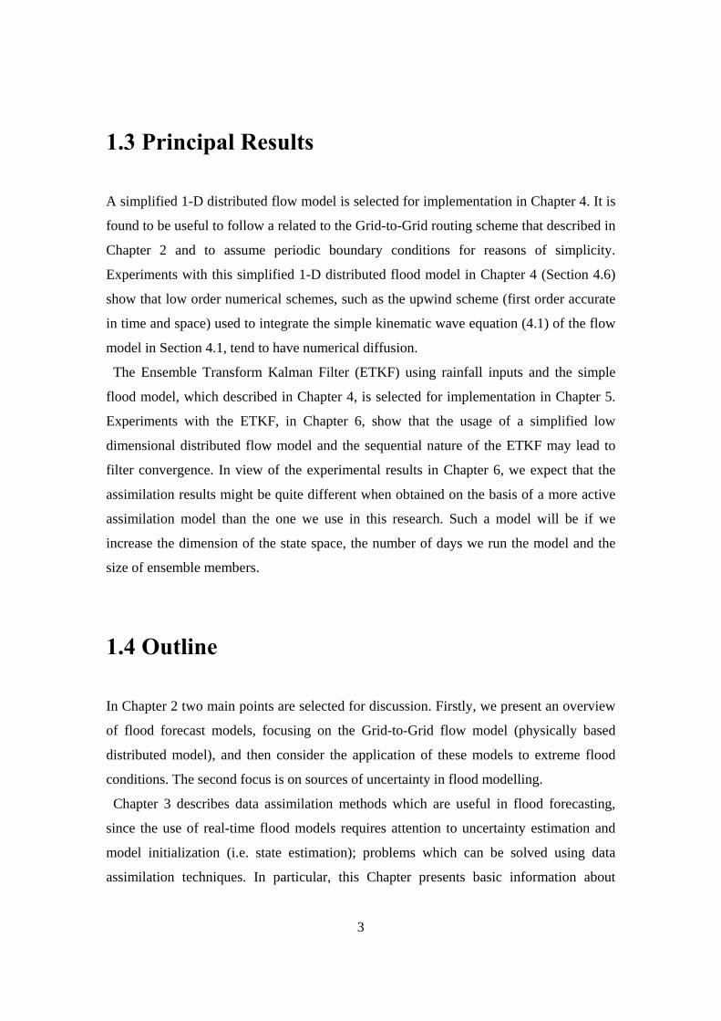
2.2.2 Maximum Water Storage Capacity

There are several different ways to calculate the maximum water storage capacity, maxS ,

for each grid-square but a simple formulation that is used by the grid-to-grid model

(Moore et al., 2006) is given mathematically by:

⎟⎟⎠

⎞⎜⎜⎝

⎛−=

maxmaxmax 1

ggcS (2.2)

for maxgg ≤ , where g is the average topographic gradient, maxg is the upper limit of

gradient and maxc is the upper limit of storage capacity. The last two parameters act as

regional parameters for the runoff production process and that allows the values of the

structural parameter, maxS , to be determined using only these two. This simple scheme

does not take account of soil, geology and land cover properties.

More complex formulations aim to allow the use of soil, geology and terrain properties

as a part of the flood forecasting process. These take account of the lateral drainage, the

groundwater flow, the percolation and the volume of soil water and groundwater.

Examples of such schemes are given by Moore et al., (2006).

11

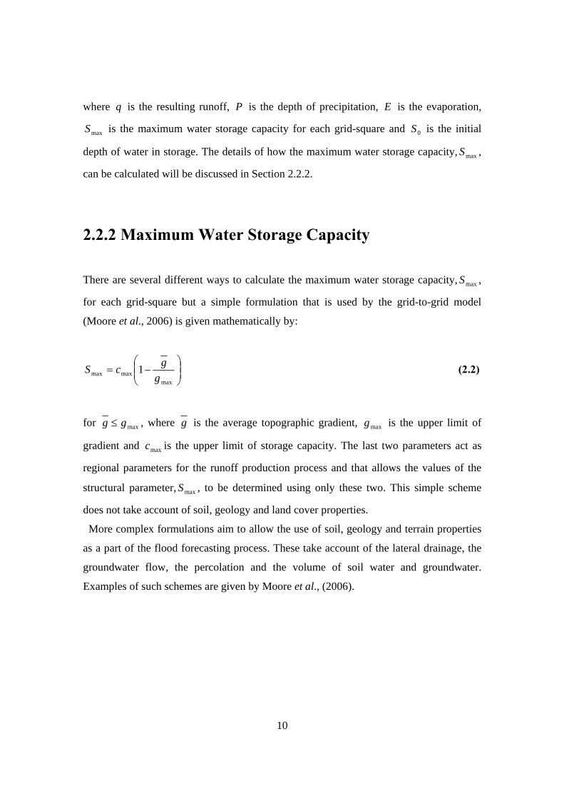
2.2.3 Grid-to-Grid Flow Routing

In the Grid-to-Grid flow model the runoff production is routed by using the simple

kinematic wave equation:

)( Rucxqc

tq

+=∂∂

+∂∂ (2.3)

where q is the channel flow, c is the kinematic wave speed, u is the lateral inflow per

unit length of river and R is the return flow.

The flood model is applied separately in two different layers, as figure 2.3 shows. In this

case there are two pathways of water movement, one on the surface (fast) and one on the

sub-surface (slow). Assuming different wave speeds, c , over surface and sub-surface as

well as over land and river, the water is transferred from one grid cell to another.

Mathematically in one dimension the difference between the parallel fast and slow

pathways of water movement is expressed by the following equations:

Over land: )( llll

ll Ruc

xq

ct

q+=

∂∂

+∂∂

, (2.3.1)

)( llblblb

lblb Ruc

xq

ct

q−=

∂∂

+∂∂

, (2.3.2)

Over river: )( rrrr

rr Ruc

xq

ct

q+=

∂∂

+∂∂ , (2.3.3)

)( rrbrbrb

rbrb Ruc

xq

ct

q−=

∂∂

+∂∂

, (2.3.4)

where the inflow and the return flow can vary with the surface type and pathway. As

figure 2.3 highlights, the return flow term allows for flow transfers between the sub-

surface and surface pathways to represent surface/sub-surface flow interactions on hill-

slopes and in channels and provides a regionally way of combining the fast and slow

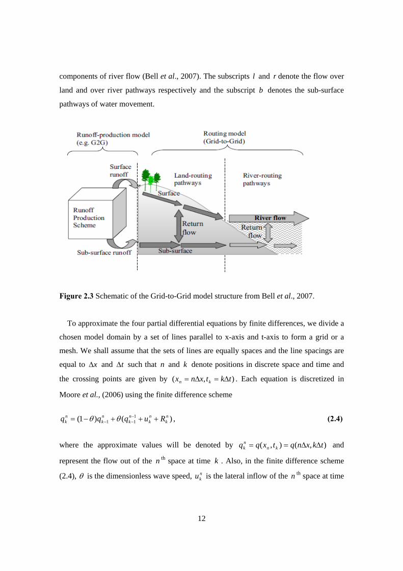
12

components of river flow (Bell et al., 2007). The subscripts l and r denote the flow over

land and over river pathways respectively and the subscript b denotes the sub-surface

pathways of water movement.

Figure 2.3 Schematic of the Grid-to-Grid model structure from Bell et al., 2007.

To approximate the four partial differential equations by finite differences, we divide a

chosen model domain by a set of lines parallel to x-axis and t-axis to form a grid or a

mesh. We shall assume that the sets of lines are equally spaces and the line spacings are

equal to x∆ and t∆ such that n and k denote positions in discrete space and time and

the crossing points are given by ),( tktxnx kn ∆=∆= . Each equation is discretized in

Moore et al., (2006) using the finite difference scheme

)()1( 111

nk

nk

nk

nk

nk Ruqqq +++−= −

−− θθ , (2.4)

where the approximate values will be denoted by ),(),( tkxnqtxqq knnk ∆∆== and

represent the flow out of the n th space at time k . Also, in the finite difference scheme

(2.4), θ is the dimensionless wave speed, nku is the lateral inflow of the n th space at time

13

k and nkR is the return flow of the n th space at time k . Equation (2.4) thus represents

flow out of the n th space at time k , nkq , as a linear weighted combination of the flow out

of the reach at the previous time 1−k , nkq 1− , the inflow to the reach from upstream at the

previous time 1−k , 11−−

nkq , and the total lateral inflow along the reach at the same time

k , where the total lateral inflow is given by the sum of lateral inflow nku and return flow

nkR (Moore et al., 2006).

However, this scheme is not consistent (we believe there is a typographical error in the

paper of Moore et al., 2006). Hence, instead we analyse a similar to the following

difference scheme,

)()1( 111

nk

nk

nk

nk

nk Rutqqq +∆++−= −

−− θθθ (2.5)

which is stable and accurate, simple and quick to run. In the finite difference scheme

(2.5), xtc

∆∆

=θ is the dimensionless wave speed and for stability we require 10 << θ .

But the most useful result of that selection is the fact that the scheme allows for different

values of the dimensionless wave speed,θ , for different pathway (surface or sub-surface)

and surface type (land or river) combinations, since θ depends on the different values of

the kinetic wave speed c . In Chapter 4, which is about the implementation of a simplified

1-D distributed flow model using similar to the grid-to-grid routing scheme, we give an

analytic description of how we determine the dimensionless wave speed θ and the order

of accuracy of the finite difference scheme.

2.2.4 Parameterization

In the grid-to-grid flood model the flow-routing and the return flow are parameterized as

water depths by Moore et al., (2006) as follows:

14

• The routing is given by: nk

nk Sq κ= , where κ is a parameter that depends on soil,

geology, terrain and land cover and nkS is the depth of water in store over the grid

square of the n th reach at time k .

• The return flow is given by: nk

nk rSR = , where r is the return flow fraction. Since

the return flow fraction is proportional to the depth of the water of the sub-surface

store, can take values between zero and one. In this case nkS represents the depth

of water in the sub-surface store of the n th reach at time k . The return flow takes

usually positive values, but it can be also negative since it represents the water

movement between the sub-surface and surface pathways and influent “stream”

conditions (Moore et al., 2006).

However, in Moore et al., (2006) paper there is no analysis of how it is possible to

parameterize the inflow as water depth. Hence, working with the same formula as above

we conclude to the next:

• The inflow is given by: nk

nk Su σ= , where σ is a parameter that depends on the

topography and nkS is the depth of water in store over the grid square of the n th

reach at time k .

2.3 Sources of Uncertainty in Flood Forecasting

The main sources of uncertainty in flood forecasting are divided in three categories in

Leahy et al., (2007):

1. Input Uncertainty of Rainfall

2. Model Uncertainty

3. Output Uncertainty

15

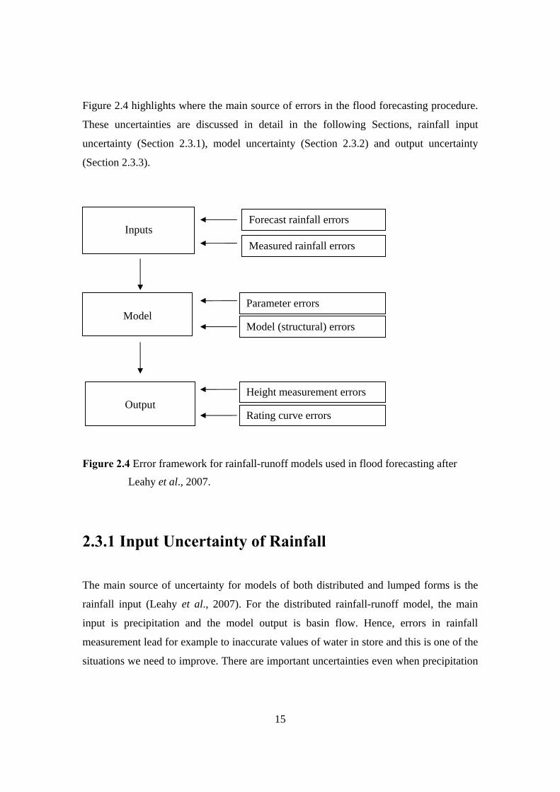
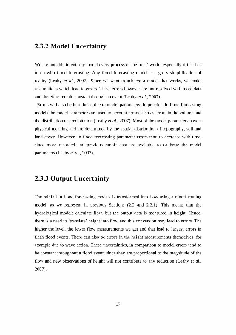
Figure 2.4 highlights where the main source of errors in the flood forecasting procedure.

These uncertainties are discussed in detail in the following Sections, rainfall input

uncertainty (Section 2.3.1), model uncertainty (Section 2.3.2) and output uncertainty

(Section 2.3.3).

Figure 2.4 Error framework for rainfall-runoff models used in flood forecasting after

Leahy et al., 2007.

2.3.1 Input Uncertainty of Rainfall

The main source of uncertainty for models of both distributed and lumped forms is the

rainfall input (Leahy et al., 2007). For the distributed rainfall-runoff model, the main

input is precipitation and the model output is basin flow. Hence, errors in rainfall

measurement lead for example to inaccurate values of water in store and this is one of the

situations we need to improve. There are important uncertainties even when precipitation

Parameter errors

Model (structural) errors

Model

Forecast rainfall errors

Measured rainfall errors

Inputs

Height measurement errors

Rating curve errors

Output

16

input to a flood forecasting model is based on recorded rainfall, since radar methods can

observe large areas but they do not directly measure rainfall (Leahy et al., 2007).

Recently, a new technique has been developed by the Met Office and CEH (Centre for

Ecology and Hydrology) to produce an ensemble rainfall forecast. This is designed to

sustain research on probabilistic flood forecasting and to take into account the uncertainty

in predicting the movement of areas of precipitation (Roberts, 2005). The ensembles are

normally developed as extensions of radar extrapolation methods, in combination with

operational Numerical Weather Prediction (NWP) forecast models, which are able to

simulate the physics and the dynamics of the atmosphere and hence to initiate

precipitation. In particular, Numerical Weather Prediction (NWP) model outputs are used

to forecast rainfall. In these models the grid size is often larger than the one in flood

forecasting models and hence small errors in the location of the weather systems by NWP

models may result in inaccurate values of forecast rainfall (Leahy et al., 2007).

It is not possible to represent the exact state of the atmosphere at the start of a weather

forecast. The start of a forecast is named ‘analysis’ and for each forecast we require the

best possible ‘analysis’, since an inaccurate analysis will lead to an inaccurate forecast.

The particular difficulty we face lies in the fact that a rainfall analysis must be consistent

with the model dynamics. The analysis of a forecast must be as close as possible to

available observations (rainfall) by means of a process called data assimilation (Roberts,

2005). Data assimilation is a tool that combines observational data and numerical models

to produce an analysis which is considered as the best estimate of the current state of a

dynamical system. The details of this approach will be discussed in Chapter 3.

A particularly good way of representing forecast uncertainty is to generate probabilities

which are able to provide information in a way that is suitable for input into a rainfall-

runoff/river-flow model. Because precipitation amount is very difficult to predict

meteorologically, the uncertainty associated with any single estimate is high and varies

from case to case. To allow the forecaster to deal with the degree of uncertainty, to make

use of probabilistic flood forecasting, to formulate a scheme for processing of

information from different sources and to automate all algorithmic processing tasks are

the objectives that require much research and remains a challenge for models (Roberts,

2005).

17

2.3.2 Model Uncertainty

We are not able to entirely model every process of the ‘real’ world, especially if that has

to do with flood forecasting. Any flood forecasting model is a gross simplification of

reality (Leahy et al., 2007). Since we want to achieve a model that works, we make

assumptions which lead to errors. These errors however are not resolved with more data

and therefore remain constant through an event (Leahy et al., 2007).

Errors will also be introduced due to model parameters. In practice, in flood forecasting

models the model parameters are used to account errors such as errors in the volume and

the distribution of precipitation (Leahy et al., 2007). Most of the model parameters have a

physical meaning and are determined by the spatial distribution of topography, soil and

land cover. However, in flood forecasting parameter errors tend to decrease with time,

since more recorded and previous runoff data are available to calibrate the model

parameters (Leahy et al., 2007).

2.3.3 Output Uncertainty

The rainfall in flood forecasting models is transformed into flow using a runoff routing

model, as we represent in previous Sections (2.2 and 2.2.1). This means that the

hydrological models calculate flow, but the output data is measured in height. Hence,

there is a need to ‘translate’ height into flow and this conversion may lead to errors. The

higher the level, the fewer flow measurements we get and that lead to largest errors in

flash flood events. There can also be errors in the height measurements themselves, for

example due to wave action. These uncertainties, in comparison to model errors tend to

be constant throughout a flood event, since they are proportional to the magnitude of the

flow and new observations of height will not contribute to any reduction (Leahy et al.,

2007).

18

2.4 Case study: The Boscastle Flood

Sometimes the only indication about the precipitation in an area comes from a rainfall

radar observation a few minutes before the flood event occur and usually the information

is not available with the desired accuracy. A serious flash-flood occurred in the village of

Boscastle close to the north cost of Cornwall (SW England) on 16th August 2004. This

flash-flood associated with violent convective storms of a short duration and was the

result of a sea breeze effect. Sea breeze circulations, driven by the temperature contrast

between land and sea, led to intense thunderstorms over the area around Boscastle at

around 10.30 UTC on 16th August 2004 and continued until around 16.30 UTC.

Flooding developed from rainfall lasting for hours and occurred because the precipitation

was concentrated over the small catchment in Boscastle area (Roberts, 2005).

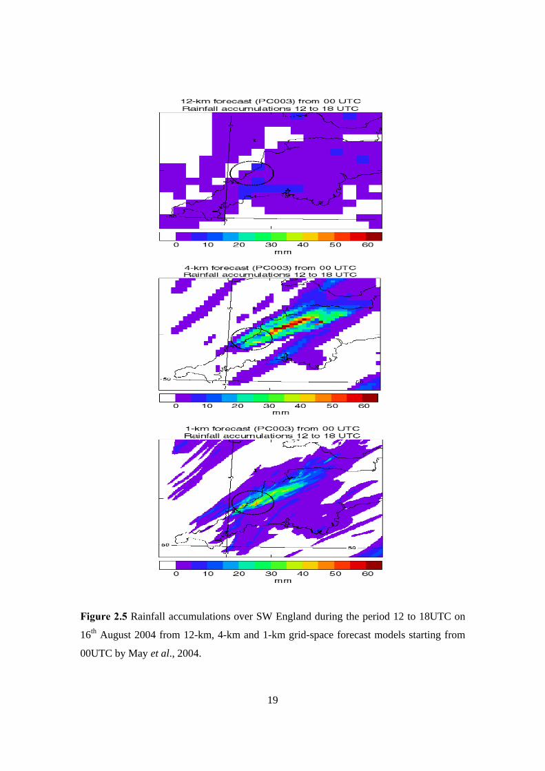
In this Section we compare three different forecasts using the 12-km, 4-km and 1-km

grid-space forecast models. Figure 2.5 shows the rainfall accumulation from 12 to

18UTC, when the highest rainfall occurred in Boscastle area. The dashed circle is a 20km

radius and is centred at the village of Boscastle (May et al., 2004). The 12-km grid-space

forecast model failed to predict the localized intense rainfall that led to flash-flood and

subsequently caused loss of life, human suffering and damage to buildings. The 4-km

grid-length model would have provided more useful guidance to forecasters, since it

produced much higher rainfall accumulations in regions near Boscastle. The first two

panels of figure 2.5 illustrate that the 4-km forecast was much better than the 12-km

forecast in predicting high rainfall accumulation, however the peak accumulations were

not in the correct location (May et al., 2004). In particular, actual peak rainfall

accumulations reached about 200mm (gauge). The 12-km grid-length model did not even

manage any accumulations greater than 10mm, in contrast to the 4-km and 1-km grid-

space forecast models (Roberts, 2005). In the 1-km forecast we observed less rain than in

the 4-km but in Boscastle area. However, the 4-km and 1-km grid-space forecast models

did predict very high accumulations, since were better able to resolve the topography and

that means that were capable to represent surface terrain much more accurately than the

12-km forecast model did.

19

Figure 2.5 Rainfall accumulations over SW England during the period 12 to 18UTC on

16th August 2004 from 12-km, 4-km and 1-km grid-space forecast models starting from

00UTC by May et al., 2004.

20

The 4-km grid-length forecast model was able to resolve the thunderstorms and the

complex flow around the coast. On the other hand, the 1-km grid-space forecast model

was able to resolve the showers and the local orography more accurately (May et al.,

2004). Finally, the 12-km forecast model was unable to represent the catchment properly

and did not indicate greater average values over the catchments in the area of Boscastle.

Hence, the 4 and 1-km grid-space models, as described before, were much better and did

predict higher average rainfall accumulations over catchments in the vicinity of

Boscastle, though without indicating a serious flood risk (Roberts, 2005).

In observe, a 4-km grid-length model is more practicable than a 1-km model but a major

advantage a 1-km grid-space model has over the 12-km and 4-km grid-length models is

the fact that allows the simulation of rainfall rates that can be directly compared with

those measured by radar and rain gauges. In this case, is given the possibility to make

direct use of model output to warn of local flood risk. But locations, timings and rainfall

rates may be wrong and this can be crucial for flood prediction, particularly for small

catchments such as Boscastle. Finally, denser grid spacing like the grid spacing of 1-km

can include and develop more accurately representation of cloud structure and

precipitation and hence to give more realistic simulations of extreme storms (Roberts,

2005).

The purpose of combining these three forecasts can be a more realistic view of the

forecast uncertainty (Roberts, 2005). Figure 2.5 illustrates that a combination of forecasts

picked out the vicinity of Boscastle as being more at flood risk than elsewhere. The

Boscastle flood was one of the serious examples, occurred in England, of a flash-flood

caused by rain from localized thunderstorms falling into a small river in a fast response

catchment (Roberts, 2005). Recently, a framework for extreme flood forecasting has been

set down and developed. This framework (see, e.g., Moore et al., 2006) in the beginning

selects different meteorological information and then identifies case study catchments

that they may affect. The case studies have given examples of successful high-resolution

forecasts of extreme flood producing situations. However, until now we do not really

know how accurate a high resolution forecast of a severe event is to small changes in

initial conditions.

21

2.5 Summary

This Chapter has demonstrated the need to improve the flood forecasting models (lumped

conceptual and physically based distributed models) and warning, since floods cause loss

of life, human suffering and economic hardship due to rebuilding costs. The distributed

Grid-to-Grid model (Section 2.2) show promise in providing an integrated approach to

modelling for any location and since there is uncertainty associated with rainfall forecasts

whatever the resolution of the flood forecasting model; the Grid-to-Grid model needs

improvement.

The main sources of uncertainty in flood modelling are divided in three categories by

Leahy et al., (2007): input uncertainty of rainfall (Section 2.3.1), model uncertainty

(Section 2.3.2) and output uncertainty (Section 2.3.3). An ensemble approach has been

developed to try and deal with rainfall uncertainty, by using ensemble rainfall forecasts as

an input to an ensemble flood model. It seems natural to combine this approach with an

ensemble data assimilation system. These ideas are discussed in Chapter 3. Finally, in

Section 2.4 is demonstrated a serious flash-flood event which occurred in Boscastle (SW

England). This extreme flood was a result of errors in Numerical Weather Prediction

(NWP) products which used as rainfall inputs in flood forecasting models and led in

uncertainties in flood forecasting. The use of ensemble rainfall forecasts in conjunction

with sophisticated model initialization methods is the focus of Chapter 3.

22

Chapter 3

Ensemble Flood Forecasting

In Chapter 2 was mentioned that the use of real-time flood models requires attention to

uncertainty estimation and model initialization (i.e. state estimation). Knowledge of the

uncertainty in flood forecasting and resulting flood warnings, especially in flood risk

areas, has become of interest the last decade (Zappa et al., 2008). Model initialization and

updating of distributed flood models is not yet well established, compared to lumped

conceptual models. For that reason, there is a pressing need to look at forecast updating

methods such the state-correction (Moore et al., 2006).

The basic subject of this Chapter is the description of data assimilation methods which

are useful in solving the aforementioned problems in flood forecasting. In particular, this

Chapter presents basic information about ensemble forecasting, data assimilation and

describes the techniques of Kalman and Ensemble Kalman Filters.

3.1 Rainfall Inputs

Rainfall inputs are the main source of uncertainty in flood forecasting models during a

flood event. One approach to reducing this uncertainty is to make use of rainfall inputs

generated from numerical weather forecasts. Implementation of an ensemble of rainfall

forecast realization inputs into a lumped conceptual flood model (PDM rainfall-runoff

model) has already been examined (Roberts, 2005). This ensemble approach of rainfall

forecasts helps to quantify the accuracy of the flow forecast and hence the likelihood of a

flood event. This is useful in issuing warnings for the risk of a flood (Pierce et al., 2005).

A new technique also, called STEPS, is a new nowcasting system under development and

23

capable of providing ensembles of rainfall forecasts (Moore et al., 2005). This technique

developed within the Gandolf and Nimrod systems (rainfall advection nowcasting

systems) to produce an ensemble of advection forecasts in which small-scale features are

replaced by random noise as the forecast progress (Roberts, 2005). This, thus, will give

the additional information of an ensemble of precipitation predictions and provide a

probabilistic forecast approach (Roberts. 2005); a more detailed review is given by

Roberts, (2005) and Moore et al., (2005).

3.2 Model Initialization

Model initialization (i.e. state estimation) and updating for lumped models are well

established, but this is more challenging for distributed models. An example of updating

methods for flood forecasting (in a lumped conceptual flood model) is given in Moore et

al., (2005). Particularly, observations of the state of the river basin, such as observations

relate to river flow, are used in real-time forecasting to improve forecast performance.

State correction is the most natural technique of forecast updating, and improvement in

model performance is given by the use of direct or related measurement of a model state.

River flow can be used to estimate a model error and provides a basis for updating the

state. For correction the model states, that are chosen, are the fast and slow response

flows from the flood model and finally the corrected flows will sum to the observed flow

(Moore et al., 2005). On the other hand, forecast updating methods in distributed flood

models (at ungauged sites) may appear limited and research is needed. Progress in these

problems may be achieved by the use of data assimilation methods, such as those used in

numerical weather prediction (Moore et al., 2005).

Data assimilation is fundamental in Numerical Weather Prediction (NWP), since it

provides and estimates initial conditions, known as the ‘analysis’ of forecast models

using physical state variables. In particular, data assimilation is a tool that combines

observational data and numerical models and tries to balance the uncertainty between

forecast and data (Kalnay, 2002). Many data assimilation techniques have their

24

foundation in Kalman filtering theory, which we will describe in subsequent Sections.

Note that the Ensemble Kalman Filter is a natural candidate for use in ensemble flood

models such as those we described above with rainfall inputs; however, unlike the

standard Kalman Filter, it has not been developed for situations where inputs play a

significant role. Hence, we will describe the ensemble filter from this literature in this

Chapter and develop it in Chapter 5 to include inputs.

3.3 The Kalman Filter

This Section introduces some notation and gives some desired properties for the Kalman

Filter. This is an established sequential data assimilation technique which is characterized

by alternate forecast and analysis steps. Generally, in the forecast step a previous state

estimate is evolved forward in time to give a forecast state at the time of the latest

observations. In the analysis step these observations are used to update the forecast state

and to determine the state of the dynamical system by giving an improved state estimate

called the ‘analysis’ (Welch & Bishop, 2006). For a detailed treatment see Welch &

Bishop, (2006).

We assume a state vector x of size n that describes the state of the forecast model. In

particular, the true state of the system at time kt will be denoted by )( kt tx . The analysis

at this time (denoted with the superscript a ) and the forecast (denoted with the

superscript f ) are given by )( ka tx and )( k

f tx respectively and are of size n . The

observation vector, of size p , at time kt will be denoted by )( kty .

We shall assume that we use random variables to model errors in the flood forecasting

model and in observations. We denote these errors tff xxe −= and taa xxe −= for the

forecast and analysis, respectively. We assume that these forecasts and analyses are

unbiased so that 0=fe and 0=ae . Finally, in this Section we will use error

covariance matrices which provide information about the size and correlation of the error

25

components and are given by Ttftff ))(( xxxxP −−= and Ttataa ))(( xxxxP −−=

(Welch & Bishop, 2006). Note that the errors and means are all for a single time kt .

3.3.1 The Kalman Filter Algorithm

The Kalman Filter (Gelb, 1974) was developed for linear dynamic systems and provided

a means of explicitly taking account of input, model and output errors (Srikanthan et al.,

2007). In this Section, we follow the description of the Kalman Filter algorithm in Welch

& Bishop, (2006). We consider the general problem of trying to estimate the state vector

x of a discrete-time controlled process (indicates that the problem is done in steps rather

than continuously). The true state of the system at the current time kt , satisfies

)()()()( 111 −−− ++= kkkt

kt tttt ηNuMxx , (3.1)

and the observation vector at the same time

)()()( kkt

k ttt εHxy += . (3.2)

In equation (3.1) M is a known matrix )( nn× which relates the state x at the previous

time 1−kt to the state at the current time kt . It is worth noting that in practice this matrix

might change with each time step, but in this description of the Kalman Filter algorithm

we assume it is constant. In the context of a flood forecasting model, state vector x will

be the river flow and the optional control input u , of size l , will denote the rainfall input.

Hence, in this equation matrix N , )( ln× , relates the rainfall input u to the river flow x .

Finally, )( 1−ktη is a Gaussian, random, unbiased and uncorrelated model noise at the

previous time 1−kt with mean zero and known covariance matrix Q (Welch & Bishop,

2006).

In equation (3.2) matrix H is a )( np× known matrix that maps state variables x to

observed variables y . An example of what an observation operator might do is the

26

interpolation from model grid to the location of an observation. Also, )( ktε is a Gaussian,

random, unbiased and uncorrelated observation noise at the same time kt with mean zero

and known covariance matrix R (the observation error covariance matrix, a )( pp×

matrix which describes the random errors in )( kty ). Note that in practice matrix H might

change with each time step or measurement, but here we assume it is constant (Welch &

Bishop, 2006). Furthermore, it is important to be mentioned that there is no correlation

between model noise and observation noise at any times (Livings, 2005).

The Kalman Filter algorithm at time kt is given by the sequence of the following

equations. In particular, the equations of the Kalman Filter divided into two groups, in the

time update equations (3.3) and (3.4) and in the measurement update equations (3.5),

(3.6) and (3.7), (Welch & Bishop, 2006).

1. State forecast: )()()( 11 −− += kka

kf ttt NuMxx . (3.3)

2. Forecast Error Covariance matrix: )()()( 11 −− += kT

ka

kf ttt QMMPP . (3.4)

3. Kalman gain matrix: 1])([)()( −+= RHHPHPK Tk

fTk

fk ttt . (3.5)

4. Analysis: )]()()[()()( kf

kkkf

ka ttttt HxyKxx −+= . (3.6)

5. Analysis Error Covariance matrix: )(])([)( kf

kka ttt PHKIP −= . (3.7)

It is important to be mentioned that the time update equations (3.3) and (3.4) evolve the

state and covariance estimates forward from time 1−kt to time kt . Matrices M and N , in

equation (3.3), are defined based on knowledge of the process, but the determination of

the process noise covariance Q , in equation (3.4), is more difficult since we normally do

not have the ability to directly observe the process we are estimating (Welch & Bishop,

27

2006). Finally, matrix )( 1−ka tP , in equation (3.4), is the ‘state error covariance matrix’

which is a )( nn× matrix and describes the random errors in the ‘initial guess’.

It is worth noting that the measurement update equations (3.5), (3.6) and (3.7) alter the

projected estimate by an actual measurement at that time (Welch & Bishop, 2006). The

first step during the measurement update is to compute the )( pn× Kalman gain matrix

K which minimizes the ‘a posteriori’ error covariance )( ka tP in equation (3.7). In the

implementation of the filter, the observation error covariance matrix R is measured prior

to operation of the filter. Measuring this matrix is usually practical and possible, since in

general we are able to take some sample measurements in order to determine the variance

of the observation noise. The following step is to calculate an ‘a posteriori’ state estimate

)( ka tx as a linear combination of an ‘a priori’ estimate )( k

f tx and a weighted

difference between the actual measurement )( kty and the measurement prediction

)( kf tHx , as given in equation (3.6). The final task of this procedure is to compute the

analysis error covariance matrix )( ka tP as given in equation (3.7). After each time and

measurement update, the same procedure is repeated with the previous ‘a posteriori’

estimates used to predict the new ‘a priori’ estimates (Welch & Bishop, 2006).

In the ‘real’ world most physical systems and models, such as the flood forecasting

models, represent nonlinearities and the Kalman Filter method is not so useful since it

works only for linear systems. For these cases, later on, Extended Kalman Filter (EKF)

methods was developed to deal with nonlinearity (Welch & Bishop, 2006). The Extended

Kalman Filter can work well, but since the nonlinearities in the flood models were

usually strong, the linearization led to inaccurate values and hence a natural framework

based on the Ensemble Kalman Filter (EnKF) has been developed for flood forecast

modelling (Srikanthan et al., 2007). Also, another reason that makes the usage of an

EnKF more useful was the computational expenses of the EKF (Srikanthan et al., 2007).

28

3.4 The Ensemble Kalman Filter

In the last decade the Ensemble Kalman Filter (EnKF) and its derivatives have been used

extensively in real time flow forecasting, especially with the Probability Distributed

Model (Moore et al., 2005). For a review of EnKF algorithms see Evensen, (2003). It is

important to be noticed, that the EnKF was not originally designed to take into account

(rainfall) inputs, but the use of EnKF allows combination of uncertainties associated with

rainfall and flood model in a systematic way in real-time flow forecasting and it has been

used by a number of researchers in the past.

The basic idea of the Ensemble Kalman Filter is to use a statistical sample of state

estimates instead of a single estimate and an error covariance matrix that measures the

uncertainty in the estimate (Livings et al., 2008). The mean of this ensemble sample

represents the ‘best’ state estimate, while the variance provides a measure of the spread

of the ensemble errors (Leahy et al., 2007). Also, with the use of a statistical sample in

EnKF algorithm we calculate the error covariance matrix from this ensemble instead of

maintaining a separate covariance matrix and that leads in a better representation of

nonlinearity and is less expensive than the Extended Kalman Filter (Evensen, 2003).

Finally, another benefit of the EnKF comes from the calculation of the Kalman gain

matrix for all statistical members which decreases the fixed cost of the additional

ensemble members (Leahy et al., 2007).

Figure 3.1 shows a schematic diagram of Ensemble Kalman Filter (EnKF), where the

uncertainty of the state is represented by the spread of the ensemble at forecast and

update steps (Leahy et al., 2007). Before we start describing the diagram, we have to

notice that the evolution model could be nonlinear and that the filter gives a reduction in

uncertainty of the estimates. In the time step 1−t the EnKF algorithm begins, where the

big blue ellipse denotes the uncertainty associated with the initial state and the red dot

denotes the unknown true state. As a starting point we chose an ensemble of state

estimates and we run the model using these statistical points and an ensemble of input for

the next time step (Leahy et al., 2007). This ensemble of state estimates is thus applied in

the nonlinear system to produce the forecast ensemble (Tippett et al., 2003). The updated

29

state from the previous time step is also used for the approximation of the probability

function of the actual state (Srikanthan et al., 2007). The light blue ellipses represent the

model state prediction with uncertainty and the pink ellipses denote the measurement

uncertainty. Finally, the Ensemble Kalman Filter combines the forecast with

measurements and then the updated state estimate, associated with uncertainty, is shown

as blue circles. During the flood event we repeat the forecast and update steps with the

sequence of the aforementioned procedure (Leahy et al., 2007). A more analytically

presentation of this process is given in Leahy et al., (2007).

Time (t)

Measurements with uncertainty

True state

Updated state estimate with uncertainty

Model state predictionwith uncertaintyInitial state

with uncertainty

True state

(t-1) (t)

(t+1)

Figure 3.1 Schematic diagram of Ensemble Kalman Filter (EnKF) from Leahy et al.,

2007.

It is worth noting that there are different types of EnKF implementation (perturbed

observation, square root etc.). In the following Sections we focus on a particular class of

ensemble filter known as Ensemble Square Root Filter (EnSRF), based on papers of

Tippett et al., (2003) and Livings et al., (2008). Finally, a specific implementation of an

EnKF; the Ensemble Transform Kalman Filter (ETKF) which based in Livings, (2005), is

given in Section 3.6 and will be also, in Chapter 5, the implementation used for the

experiments in this thesis.

30

3.4.1 Notation

The members of an ensemble sample in state space will be indicated by ix , where i

denotes the individual members of an ensemble and takes values between 1 and

N ( N indicates the size of an ensemble). We assume that the evolution of each ensemble

member is independent of all other ensemble members (Livings et al., 2008).

Subsequently, the ensemble mean will be given by

∑=

=N

iiN 1

1 xx , (3.8)

where x is an unbiased estimator of the population mean if the ensemble members ix are

drawn independently from the same probability distribution (Barlow, 1989). An initial

ensemble mean is required at time 0t equal to )( 0tx .

The ensemble perturbation matrix is of dimension )( Nn× , with n the dimension of a

state vector, and is defined by

).......(1

121 xxxxxxΧ −−−

−= NN

. (3.9)

where the x form the columns of the matrix Χ .

The ensemble covariance matrix is the )( nn× matrix given by

TN

iii

Te N

))((1

11∑=

−−−

== xxxxXXP , (3.10)

where the division by 1−N ensures that the ensemble covariance matrix eP is an

unbiased estimate (Barlow, 1989) of the state error covariance matrix P and the equality T

e ΧΧP = may be expressed by saying that Χ is a square root of eP (Tippett et al.,

2003). Note that the definition of a square root is different from the definition usually

used in mathematics; if Χ is a square root of a matrix P then PΧ =2 .

31

3.4.2 The Forecast Step

The EnKF moves sequentially from one measurement time to the next and is divided into

two steps: a forecast step and an analysis step. We start with a brief description of the

main steps of an EnKF algorithm where given an initial state )( 0tax and error covariance

matrix aP we start generating an analysis ensemble of initial states aix for Ni ≤≤1 .

This analysis ensemble will be used for the next forecast, as the starting point (Livings et

al., 2008). Then considering a nonlinear dynamical model M in the state forecast step

the ensemble is propagated forward in time using the following nonlinear model:

)())(()( 11 −− += kikaik

fi ttMt ηxx , (3.11)

where )( 1−ki tη is a pseudo-random model noise at the previous time 1−kt with known

covariance matrix Q and zero mean (Evensen, 2003). Note that the algorithm as given in

the literature does not take account of the inputs. The ensemble mean then is given by

∑=

=N

i

fi

f

N 1

1 xx , (3.12)

and the ensemble perturbation matrix by

).......(1

121

ffN

fffff

NxxxxxxΧ −−−

−= . (3.13)

Hence, the ensemble forecast error covariance matrix is defined by

Tfffe )(ΧΧP = . (3.14)

32

3.4.3 The Analysis Step

We assume in the beginning an observation y of dimension p , and an observation

operator H which maps the state vector to the observation vector. We introduce an

ensemble of forecast observation fi

fi Hxy = , where f

iy represents that observation if fix

is the true state of the system without observation noise, for Ni ≤≤1 (Livings et al.,

2008). As any other ensemble, if we assume the linear case with a linear observation

operator H , the forecast observation ensemble has an ensemble mean

ff Hxy = , (3.15)

and an ensemble perturbation matrix

ff HXY = . (3.16)

Hence, using equations (3.14) and (3.16) the Kalman gain, as in equation (3.5), will be

given by

1)( −+= RHHPHPK Tfe

Tfee

1))(()( −+= RHXHXHXX TTffTTff

1))(()( −+= RHXHXHXX TffTff

1))(()( −+= RYYYX TffTff

1)( −= SYX Tff (3.17)

where we set

RYYS += Tff )( , (3.18)

and R denotes the )( pp× observation error covariance matrix. Then the ensemble mean

updates as

33

)( fe

fa yyKxx −+= , (3.19)

and the analysis ensemble covariance matrix, using equations (3.14) and (3.17), will be

defined by

fee

ae PHKIP )( −=

TffTff )())(( 1 XXHSYXI −−=

TffTff ))()(( 1 XYSYIX −−= . (3.20)

Note that the above equations can be generalized for both linear and nonlinear

observation operators (Livings et al., 2008). Also, in practice equation (3.20) is not used

directly in Square Root Filter (SRF) implementations as will be seen in the next Section.

3.5 The Ensemble Square Root Filter

In the analysis step of an Ensemble Square Root Filter (EnSRF), the analysis state

estimate is given, as in equation (3.19), by

)( fe

fa yyKxx −+= , (3.21)

where the observation ensemble mean is equal to )( ff H xy = and the Kalman gain,

from equation (3.17), equal to 1)( −= SYXK Tffe . Note that in comparison with

equation (3.19) in the ensemble square root filter algorithm the analysis ensemble is equal

to 'i

ai xxx += , where the perturbations '

ix is the i -th column of the )( Nn× matrix

aN X1− , with aX the analysis ensemble perturbation matrix (Livings et al., 2008).

Then, the analysis perturbation equation is updated separately and is given by

TXX fa = , (3.22)

34

with T an )( NN × matrix which we want to satisfy

fTfT YSYITT 1)( −−= . (3.23)

Thus, using equations (3.22), (3.23) and (3.17), the analysis ensemble covariance matrix

Taaa )(XXP =

Tff ))(( TXTX=

TffTff ))()(( 1 XYSYIX −−=

Tffe

f ))(( XYKX −= , (3.24)

satisfies equation (3.20). From the above relationship (3.23), we can say that matrix T is

a square root of matrix fTf YSYI 1)( −− (Tippett et al., 2003). However, since matrix fTf '1' )( YSY − is difficult to compute it because we have to invert matrix S , in the next

Section we introduce a different implementation of the EnKF; the Ensemble Transform

Kalman Filter. Finally, it is important to be mentioned that matrix T is not unique and

may be replaced by TU , where U an )( NN × orthogonal matrix (Tippett et al., 2003),

where

fTfT YSYITUTU 1)()( −−= .

3.6 The Ensemble Transform Kalman Filter

The Ensemble Transform Kalman Filter (ETKF) was originally introduced in Bishop et

al., (2001) and overcomes the aforementioned difficulties in computing the analysis

update by inverting the matrix S in equation (3.23). We may verify the identity,

111 ))(()( −−− +=− fTffTf YRYIYSYI , (3.25)

35

by multiplying the left hand side of the equality with fTf YRYI 1)( −+ and using the

definition (3.18) of matrix RYYS += Tff )( . In this case is easier to compute the

)( NN × matrix fTf YRY 1)( − , since R has simpler structure (it is usually diagonal) than

S . Then the eigenvalue decomposition is given by

UΛYRY =− fTf 1)( TU , (3.26)

where U and Λ are )( NN × orthogonal and diagonal matrices respectively. Hence, we

conclude that equation (3.25) becomes

111 ))(()( −−− +=− fTffTf YRYIYSYI

UΛI += ( 1)−TU

TUΛIU 1)( −+= , (3.27)

and since from equation (3.23) fTfT YSYITT 1)( −−= we found that 21

)(−

+= ΛIUT ,

as the desired matrix square root, where ΛI + is a diagonal matrix and easy to compute.

Hence, the analysis ensemble perturbation matrix is equal to

TXX fa =

21

)(−

+= ΛIUX f .

After implementation of the Ensemble Transform Kalman Filter (ETKF) by Livings et

al., (2008) and after the suggestion of Wang et al., (2004) for a new filter, the Revised

ETKF, was found that we take better results if matrix T is equal to

TUΛIUT 21

)(−

+= , (3.28)

which is now a symmetric matrix, since TU is orthogonal. With that assumption the

Revised ETKF is unbiased, from Theorem 2 of Livings et al., (2008) and the updated

ensemble perturbation matrix is finally given by

36

TXX fa =

Tf UΛIUX 21

)(−

+= . (3.29)

3.7 Summary

In Chapter 3 was presented basic information about ensemble forecasting, considering the

model initialization problems in Section 3.2. An introduction to data assimilation

methods and how we can relate them with flood forecasting models is provided by the

Kalman Filter description in Section 3.3. This sequential data assimilation technique

developed for linear dynamic systems and provided a means of explicitly taking account

of input, model and output uncertainties. For nonlinear dynamic systems Ensemble

Kalman Filter (EnKF) techniques were presented in Section 3.4 which provide an

alternative method of estimating these uncertainties by the use of an ensemble of state

estimates instead of a single state estimate and without maintaining a separate error

covariance matrix. The basic idea of this Chapter was to represent sequential data

assimilation techniques useful in solving the initialization problem in flood forecasting

models. For that reason, in Section 3.5 described the Ensemble Square Root Filter and

later in Section 3.6 an Ensemble Transform Kalman Filter (ETKF) algorithm which is an

ensemble approach that developed to try and deal with rainfall uncertainty, as we will see

in Chapter 5.

The following Chapter discusses the selection of a simplified one-dimensional (1-D)

distributed flood forecasting model for implementation. It describes also some problems

that were encountered in implementing the simplified 1-D distributed flow model using a

finite difference scheme similar to the Grid-to-Grid routing scheme that was presented in

Chapter 2, and the solutions that were accepted by representing basic experimental

results.

37

Chapter 4

A Simplified 1-D Distributed Flow Model

This Chapter is about the implementation of a simplified one-dimensional (1-D)

distributed flow model and the presentation of basic validation results. The experiments

with the simple flood model differ in the time and length scale and in the values of model

parameters.

4.1 Simplified Distributed Flow Routing

The simplified 1-D distributed flood model we will present in this Chapter is a new

simple flow model that we developed. Our simplified 1-D distributed flow model is

related to the routing scheme that described in Section 2.2.3. The basis of the distributed

flow routing scheme is the simple kinematic wave equation

)( EPaxqc

tq

−=∂∂

+∂∂ , (4.1)

where in the left hand side of equation (4.1), t and x denote time and space respectively,

q represents the channel flow and c the kinematic wave speed. In the right hand side of

equation (4.1), a is a parameter which could depend on the soil, geology, terrain and

land cover, P is the rainfall rate and E is the evaporation rate. In Table 4.1 we give the

dimensions of these physical parameters, where L and T denote the length scale and

time scale, respectively. However, for the rest of this thesis, we assume that the equation

(4.1) and the functions of precipitation and evaporation as given in Section 4.2 have been

non-dimensionalized. It is worth to be mentioned that the left hand side of equation (4.1)

38

comes from the left hand side of the simple kinematic wave equation (2.3), which is used

as the basis for the Grid-to-Grid routing scheme. The right hand side of equation (4.1)

was chosen equal to )( EPa − for reasons of simplicity. Note that this allows us to

calculate the analytic solution of equation (4.1), as we will describe in Section 4.2.

Parameter name Dimensions Description

Channel flow rate: q TL /3 River flow Kinetic wave speed: c TL / Related to the flow velocity

Parameter a T/1 Could depend on soil, land cover etc.

Precipitation rate: P TL /3 Rainfall input Evaporation rate: E TL /3 Rainfall loss

Table 4.1 Routing model parameters.

We solve equation (4.1) for channel flow ),( txq on the domain π20 ≤≤ x , 0≥t with

an initial condition given by

)()0,( xfxq = , π20 ≤≤ x (4.2)

for a smooth, periodic function )(xf , such that )2()( π+= xfxf .

Our solution also satisfies periodic boundary conditions,

),2(),( txqtxq π+= . (4.3) Note that the assumption of periodic boundary conditions is not very realistic, since few

rivers have a loop shape. However, we have chosen these conditions to make our flow

model easier to implement numerically.

39

4.2 Analytic Solution

In this Section we present the analytic solution of equation (4.1) for specific functions of

the initial condition, the precipitation P and the evaporation E . Our choice of initial

condition for this particular problem is given by

)()0,( xfxq =

)sin(1 x+= , (4.4) for π20 ≤≤ x . Then, we distribute precipitation and evaporation over the hours of day

and we assume that the precipitation P is changing over time with the following function

)sin(1)( δ++= wttP , (4.5)

which is a time varying function with w the frequency of rainfall and δ the phase. The

above assumption for precipitation P is not very realistic, but the simple function we

chose is useful for the calculation of the analytic solution, to enable us to validate the

code. We assume that time 0=t corresponds to midnight on the first day ( 1=t is

midnight on the second day) and each time unit corresponds to 24 hours. The first panel

of figure 4.1 shows the evolution of precipitation during the hours of daylight and

darkness. Usually, in countries such as England and Northern European countries,

precipitation events occur, during the summer, late in the evening (for examples of flash

flood events see Roberts, 2005). Hence, for the case of precipitation we chose the phase

πδ = , since we wanted to achieve the peak of the rainfall later in the evening during the

summer. As figure 4.1 illustrates, the peak of the rainfall during the hours of daylight is

nearly at 18UTC (near to 0.8) at the evening. Finally, considering that evaporation E

varies sinusoidally (Moore & Weiss, 1980), it is then given by

)sin(05.0)( γβ ++= zttE , (4.6)

which is also a time varying function with β a parameter that shows the magnitude of

the evaporation during the day, z the frequency of the evaporation and γ the phase. For

40

that case, we chose the phase 4/5πγ = , since we wanted to achieve the peak of the

evaporation, as the second panel of figure 4.1 shows, nearly at 15UTC (near to 0.6) in the

afternoon. Note that in the practical real-time circumstances rainfall and evaporation are

very difficult to be measured.

It is worth to be mentioned the fact that we assume for this flood model that the values

of rainfall are twenty times more than the values of evaporation during one day. With this

assumption we expect, by running the simplified 1-D distributed flow model for more

than 4 days, to observe bigger values of river flow for the last experimental days than for

the first day.

0 0.1 0.2 0.3 0.4 0.5 0.6 0.7 0.8 0.9 10

1

2

Time (Days)

Prec

ipita

tion

Rainfall during 1 day

0 0.1 0.2 0.3 0.4 0.5 0.6 0.7 0.8 0.9 10

0.05

0.1

Time (Days)

Evap

orat

ion

Evaporation during 1 day

Figure 4.1 The evolution of precipitation and evaporation over the hours of daylight and

darkness.

To find out the analytic solution of the distributed flow routing scheme (4.1) we use the

method of characteristics (Scott, 2003) of the first-order partial differential equations

(PDEs). The key idea is to change coordinate system from ),( tx to a new one ),( 0 sx in

which PDE (4.1) becomes an ordinary differential equation (ODE) along appropriate

curves, named ‘characteristic curves’, in the tx − plane. The new variable 0x will be

41

constant along the characteristics and will be points along the 0=t axis in the tx −

plane; on the other hand the new variable s will vary along the characteristic line. If, we

use the form

))(),((),( stsxqtxq = , where ))(),(( stsx is a characteristic line we have, using the chain rule, that

dsdt

tq

dsdx

xqstsxq

dsd

∂∂

+∂∂

=))(),(( . (4.7)

The left hand side of the PDE (4.1) is given if we set cdsdx

= and 1=dsdt ; the right hand

side of equation (4.1) is given if we set )( EPadsdq

−= . Thus, to find the solution of the

PDE we have to solve these ODEs. We start by taking

1=dsdt , (4.8)

with initial condition 0)0( =t and we obtain that st = . Then solving

cdsdx

= , (4.9)

with initial condition 0)0( xx = we can easily observe that 0xcsx += which implies that

0xctx += , which is the characteristic curve and 0x is the point where each curve

intersects the x - axis in the tx − plane. Finally, by taking

)( EPadsdq

−= ,

and using the functions for precipitation P (4.5) and evaporation E (4.6), as defined

before, we have that

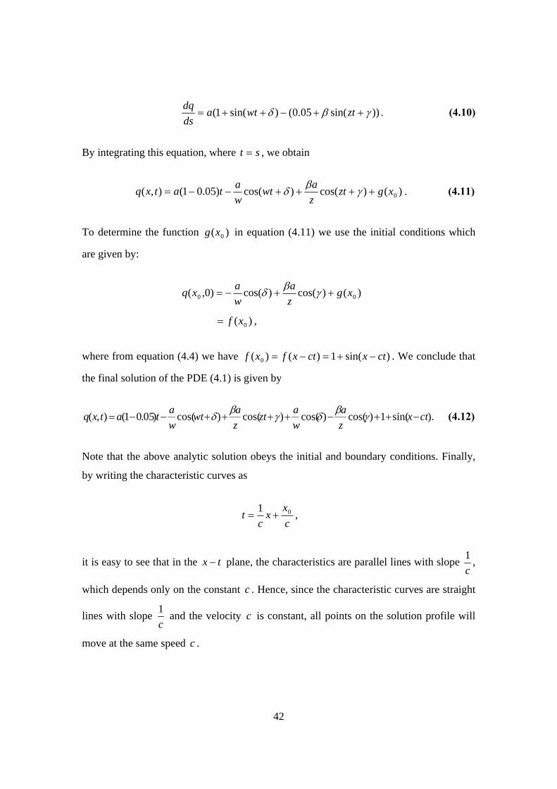
42

))sin(05.0()sin(1( γβδ ++−++= ztwtadsdq . (4.10)

By integrating this equation, where st = , we obtain

)()cos()cos()05.01(),( 0xgztzawt

watatxq ++++−−= γβδ . (4.11)

To determine the function )( 0xg in equation (4.11) we use the initial conditions which

are given by:

)()cos()cos()0,( 00 xgza

waxq ++−= γβδ

)( 0xf= ,

where from equation (4.4) we have )sin(1)()( 0 ctxctxfxf −+=−= . We conclude that

the final solution of the PDE (4.1) is given by

).sin(1)cos()cos()cos()cos()05.01(),( ctxza

wazt

zawt

watatxq −++−++++−−= γβδγβδ (4.12)

Note that the above analytic solution obeys the initial and boundary conditions. Finally,

by writing the characteristic curves as

cx

xc

t 01+= ,

it is easy to see that in the tx − plane, the characteristics are parallel lines with slope c1 ,

which depends only on the constant c . Hence, since the characteristic curves are straight

lines with slope c1 and the velocity c is constant, all points on the solution profile will

move at the same speed c .

43

4.3 Numerical Implementation

To approximate the partial differential equation (4.1) by finite differences, we divide a

chosen model domain by a set of lines parallel to x-axis and t-axis to form a grid. We

assume that the sets of lines are equally spaced and the line spacings are equal to x∆ and

t∆ . Then the crossing points are given by ),( tktxnx kn ∆=∆= , such that n and k denote

positions in discrete space and time respectively, and we seek approximations of the

solution at these grid points. These approximate values will be denoted by

),(),( tkxnqtxqq knnk ∆∆==

and represent the flow out of the n th reach at time k . We apply that one dimensional

flood model in one layer where it performs routing of channel flow using the kinematic

assumption. In this case there is only one pathway of water movement, on the surface.

Also, in the beginning as a simple example, precipitation, evaporation and routing

parameters are considered to be spatially uniform over the area corresponded to a channel

plane, but generally may vary from plane to plane. We choose the upwind scheme (explicit finite difference scheme) to discretize equation

(4.1) and we first consider the following simple approximations of the time and space

derivatives. The approximation of the time derivative of equation (4.1) is given by:

tqq

txtq n

knk

kn ∆−

≈∂∂ −1),( , (4.13)

and the approximation of the space derivative by:

xqq

txxq n

knk

kn ∆−

≈∂∂ −

−−111),( . (4.14)

Using equations (4.13) and (4.14), we have that the simple kinematic wave equation (4.1)

is approximated as:

44

)(1111 n

kn

k

nk

nk

nk

nk EPa

xqq

ctqq

−=∆−

+∆− −

−−− , (4.15)

and finally, from the above equation, we obtain the following finite difference

representation for the approximate values at time k :

)()1( 111

nk

nk

nk

nk

nk EPtaqqq −∆++−= −

−− θθ , (4.16)

where θ is the dimensionless wave speed equal to xtc

∆∆

=θ , nkP and n

kE represent the

precipitation and the evaporation of the n th space at time k , respectively.

4.4 Accuracy of the finite difference scheme

To determine the order of accuracy of equation (4.15) we use the truncation error which

defined by

)(1111 n

kn

k

nk

nk

nk

nkn

k EPaxqq

ctqq

−−∆−

+∆−

=−−−−τ . (4.17)

Assuming that the channel flow q , the precipitation P and the evaporation E are

smooth functions of space and time, we expand in Taylor series about ),( 1−kn tx in

powers of x∆ and t∆ :

qtxqttxqtkxnqq knknnk ≡=∆−=∆−∆= −− ),(),())1(,( 11 (4.18)

),(),(),( 1 ttxqtttxqtkxnqq knknnk ∆+=∆+∆−=∆∆= −

)(),(!3

),(!2

),(),( 41

3

1

2

11 ttxqttxqttxtqtxq kntttknttkntkn ∆Ο+∆

+∆

+∆+= −−−−

)(62

432

tqtqttqq tttttt ∆Ο+∆

+∆

+∆+= (4.19)

45

),(),())1(,)1(( 111 −−− ∆−=∆−∆−=∆−∆−= knkn

nk txxqttxxqtkxnqq

)(),(!3

),(!2

),(),( 41

3

1

2

11 xtxqxtxqxtxxqtxq knxxxknxxknxkn ∆Ο+∆

−∆

+∆−= −−−−

)(62

432

xqxqxxqq xxxxxx ∆Ο+∆

−∆

+∆−= (4.20)

),(),(),( 1 ttxPtttxPtkxnPP knkn

nk ∆+=∆+∆−=∆∆= −

)(),(!3

),(!2

),(),( 41

3

1

2

11 ttxPttxPttxtPtxP kntttknttkntkn ∆Ο+∆

+∆

+∆+= −−−−

)(62

432

tPtPttPP tttttt ∆Ο+∆

+∆

+∆+= (4.21)

),(),(),( 1 ttxEtttxEtkxnEE knknnk ∆+=∆+∆−=∆∆= −

)(),(!3

),(!2

),(),( 41

3

1

2

11 ttxEttxEttxtEtxE kntttknttkntkn ∆Ο+∆

+∆

+∆+= −−−−

)(62

432

tEtEttEE tttttt ∆Ο+∆

+∆

+∆+= (4.22)

We can make the substitution of equations (4.18), (4.19), (4.20), (4.21) and (4.22) into

the truncation error nkτ (4.17) and cancel:

⎥⎦

⎤⎢⎣

⎡−∆Ο+

∆+

∆+∆+

∆= qtqtqttqq

t ttttttnk )(

621 4

32

τ

⎥⎥⎦

⎤

⎢⎢⎣

⎡⎟⎟⎠

⎞⎜⎜⎝

⎛∆Ο+

∆−

∆+∆−−

∆+ )(

624

32

xqxqxxqqqx

cxxxxxx

⎢⎣

⎡∆Ο+

∆+

∆+∆+− )(

624

32

tPtPttPPa tttttt

⎥⎦

⎤⎟⎟⎠

⎞⎜⎜⎝

⎛∆Ο+

∆+

∆+∆+− )(

624

32

tEtEttEE tttttt

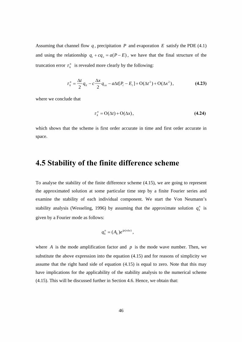
46

Assuming that channel flow q , precipitation P and evaporation E satisfy the PDE (4.1)

and using the relationship )( EPacqq xt −=+ , we have that the final structure of the

truncation error nkτ is revealed more clearly by the following:

)()(][22

22 xtEPtaqxcqtttxxtt

nk ∆Ο+∆Ο+−∆−

∆−

∆=τ , (4.23)

where we conclude that

)()( xtnk ∆Ο+∆Ο=τ , (4.24)

which shows that the scheme is first order accurate in time and first order accurate in

space.

4.5 Stability of the finite difference scheme

To analyse the stability of the finite difference scheme (4.15), we are going to represent

the approximated solution at some particular time step by a finite Fourier series and

examine the stability of each individual component. We start the Von Neumann’s

stability analysis (Wesseling, 1996) by assuming that the approximate solution nkq is

given by a Fourier mode as follows:

)()( xnipk

nk eAq ∆= ,

where A is the mode amplification factor and p is the mode wave number. Then, we

substitute the above expression into the equation (4.15) and for reasons of simplicity we

assume that the right hand side of equation (4.15) is equal to zero. Note that this may

have implications for the applicability of the stability analysis to the numerical scheme

(4.15). This will be discussed further in Section 4.6. Hence, we obtain that:

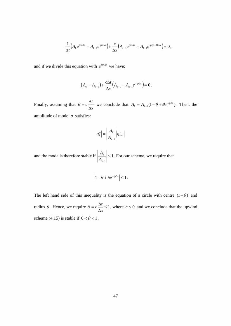
47

( ) ( ) 01 )1(111 =−

∆+−

∆∆−

−∆

−∆

−∆ xnip

kxipn

kxipn

kxipn

k eAeAx

ceAeAt

,

and if we divide this equation with xipne ∆ we have:

( ) ( ) 0111 =−∆∆

+− ∆−−−−

xipkkkk eAA

xtcAA .

Finally, assuming that xtc

∆∆

=θ we conclude that )1(1xip

kk eAA ∆−− +−= θθ . Then, the

amplitude of mode p satisfies:

nk

k

knk q

AA

q 11

−−

=

and the mode is therefore stable if 11

≤−k

k

AA

. For our scheme, we require that

11 ≤+− ∆− xipeθθ .

The left hand side of this inequality is the equation of a circle with centre )1( θ− and

radius θ . Hence, we require 1≤∆∆

=xtcθ , where 0>c and we conclude that the upwind

scheme (4.15) is stable if 10 << θ .

48

4.6 Validation of the numerical implementation

Since so far we gave an analytic description of the simplified 1-D distributed flow model

methodology, we have also in this Section to give some basic validation results. Before

we start describing the modelling process and giving some experimental results we need

to describe how we chose the initial conditions and the model parameters in the

implemented flow model.

Following the process of the simplified distributed flow routing described in Section 4.1

all the experiments were carried out using a MATLAB code. To start the calculations we

take the initial condition, precipitation and evaporation as equations (4.4), (4.5) and (4.6)

respectively, in Section 4.2, so that we can evaluate the numerical model’s performance

against an analytic solution. Then, if we carry out a calculation in a periodic domain, with

period π2 , we soon discover that the experimental results depend critically on the values

of t∆ , x∆ , c and a . The entire space has divided into discrete intervals x∆ , which are

taken equal to π2 /(number of space grid points). We first divide the entire space into 40

grid points ( 1571.0=∆x ) and then into 150 and 450 grids. For these specific state space

dimensions the flow model has been trialled for different times (days) of time interval

01.0=∆t and for different values of model parameters. These different trials of the flow

model help us understand how easily and widely the simplified distributed flood model

could be applied to address the ungauged forecasting problem at any location within a

chosen domain (Moore et al., 2006). It is worth noting that longer time steps (than

01.0=∆t ) and longer space steps (than 0140.0=∆x ) are more economical but less

accurate, so the choice in this research involves dealing with the trade-off between

accuracy and efficiency.

Topographic feature such as slope, aspects etc. are important to determine direction of

grid flow. Soil, geology and land cover features are also important in determining the

rainfall loss-evaporation. Soil, geology and land cover properties are taken account in our

model by using parameter a in the simple kinematic wave equation (4.1). That has both

disadvantages, since we do not have ‘reliable’ soil/geology information to run the flow

model and advantages, since the resulting model requires only a small number of regional

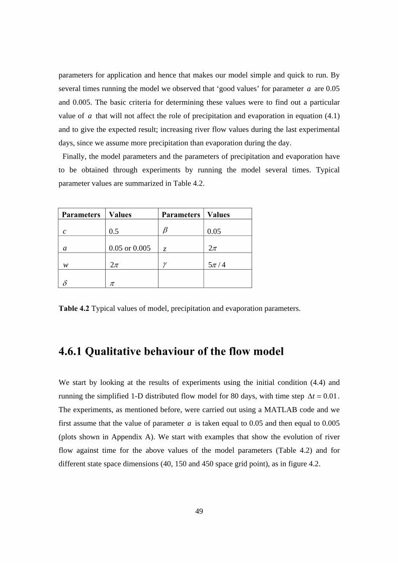
49

parameters for application and hence that makes our model simple and quick to run. By

several times running the model we observed that ‘good values’ for parameter a are 0.05

and 0.005. The basic criteria for determining these values were to find out a particular

value of a that will not affect the role of precipitation and evaporation in equation (4.1)

and to give the expected result; increasing river flow values during the last experimental

days, since we assume more precipitation than evaporation during the day.

Finally, the model parameters and the parameters of precipitation and evaporation have

to be obtained through experiments by running the model several times. Typical

parameter values are summarized in Table 4.2.

Parameters Values Parameters Values c 0.5 β 0.05 a 0.05 or 0.005 z π2 w π2 γ 4/5π δ π

Table 4.2 Typical values of model, precipitation and evaporation parameters.

4.6.1 Qualitative behaviour of the flow model

We start by looking at the results of experiments using the initial condition (4.4) and

running the simplified 1-D distributed flow model for 80 days, with time step 01.0=∆t .

The experiments, as mentioned before, were carried out using a MATLAB code and we

first assume that the value of parameter a is taken equal to 0.05 and then equal to 0.005

(plots shown in Appendix A). We start with examples that show the evolution of river

flow against time for the above values of the model parameters (Table 4.2) and for

different state space dimensions (40, 150 and 450 space grid point), as in figure 4.2.

50

In this figure we give analytic and approximate solutions of equation (4.1) by running

the flood model for different values of x∆ . In each panel, along the x-axis we plot the

time (days) and in y-axis the river flow (volume/time). The first panel in figure 4.2 shows

the analytic solution (4.12) obtained as we described in Section 4.2. The second panel

(a.) gives the numerical solution of the finite difference scheme (4.16) in a periodic

domain with period π2 , for state space dimension equal to 40. The third (b.) and the

fourth (c.) panel illustrate again the approximate solution but for different number of

space grid points; 150 and 450 grids respectively. These are examples of the evolution of

the flow model subject to a small number (40), to a medium number (150) and a large

number (450) of space grid points, since we want to show the problems that we face with

the numerical diffusion for small state space dimension. Note that the river flow values

are taken at a specific grid point. However, the behaviour is qualitatively similar at all

grid points.

These experiments have revealed two main points. Firstly, we are able to see that the

river flow (and the error also) increases with time. This is to be expected since the rain-

rate is twenty times larger than the evaporation rate. The most important result of this

experiment in figure 4.2 has to do with the numerical diffusion. As we can see in the

second panel (a.) for number of grid points equal to 40 the approximate solution behaves

differently from the analytic solution. The amplitude of the river flow oscillations

decreases. This is a consequence of the use of our numerical scheme, which has a

diffusive character (Morton & Mayers, 2005). In Section 4.3, we discussed that time and

space are divided into a discrete grid and the simple kinematic wave equation (4.1) is

discretized into finite difference equation (4.15), which in general is more diffusive than

the original differential equation (4.12). Consequently, the approximate solution behaves

differently from the analytic solution, since the simulated system depends on the type of

discretization that is used, which is the upwind scheme. This scheme is first order

accurate in time and space and that is one of the reasons that cause numerical diffusion

(Morton & Mayers, 2005) especially if we run the flood model for small number of space

grid points and for more than 30 days. Usually, higher order numerical methods tend to

have less numerical diffusion than low order numerical schemes, such as the upwind

scheme that we use in these experiments. As noted by Morton & Mayers, (2005), one of

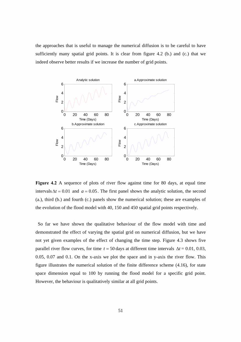
51

the approaches that is useful to manage the numerical diffusion is to be careful to have

sufficiently many spatial grid points. It is clear from figure 4.2 (b.) and (c.) that we

indeed observe better results if we increase the number of grid points.

0 20 40 60 800

2

4

6

Time (Days)

Flow

Analytic solution

0 20 40 60 800

2

4

6

Time (Days)Fl

ow

a.Approximate solution

0 20 40 60 800

2

4

6

Time (Days)

Flow

b.Approximate solution

0 20 40 60 800

2

4

6

Time (Days)

Flow

c.Approximate solution

Figure 4.2 A sequence of plots of river flow against time for 80 days, at equal time

intervals 01.0=∆t and 05.0=a . The first panel shows the analytic solution, the second

(a.), third (b.) and fourth (c.) panels show the numerical solution; these are examples of

the evolution of the flood model with 40, 150 and 450 spatial grid points respectively.

So far we have shown the qualitative behaviour of the flow model with time and

demonstrated the effect of varying the spatial grid on numerical diffusion, but we have

not yet given examples of the effect of changing the time step. Figure 4.3 shows five

parallel river flow curves, for time 50=t days at different time intervals t∆ = 0.01, 0.03,

0.05, 0.07 and 0.1. On the x-axis we plot the space and in y-axis the river flow. This

figure illustrates the numerical solution of the finite difference scheme (4.16), for state

space dimension equal to 100 by running the flood model for a specific grid point.

However, the behaviour is qualitatively similar at all grid points.

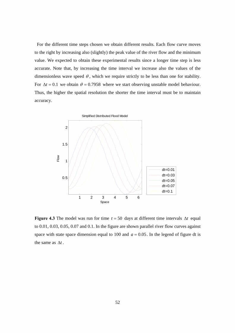
52

For the different time steps chosen we obtain different results. Each flow curve moves

to the right by increasing also (slightly) the peak value of the river flow and the minimum

value. We expected to obtain these experimental results since a longer time step is less

accurate. Note that, by increasing the time interval we increase also the values of the

dimensionless wave speed θ , which we require strictly to be less than one for stability.

For 1.0=∆t we obtain 7958.0=θ where we start observing unstable model behaviour.

Thus, the higher the spatial resolution the shorter the time interval must be to maintain

accuracy.

1 2 3 4 5 6

0.5

1

1.5

2

Space

Flow

Simplif ied Distributed Flood Model

dt=0.01dt=0.03dt=0.05dt=0.07dt=0.1

Figure 4.3 The model was run for time 50=t days at different time intervals t∆ equal

to 0.01, 0.03, 0.05, 0.07 and 0.1. In the figure are shown parallel river flow curves against

space with state space dimension equal to 100 and 05.0=a . In the legend of figure dt is

the same as t∆ .

53

4.6.2 Validation of the flow model

Our basic measure of estimation error is the difference between the exact solution and the

approximate solution at any given time and space. A suitable spatially averaged version

of this measure is the root-mean-square (rms) error averaged over all the grid points in

the domain.

In the first panel of figure 4.4, we plot log(rms-error) against )log( t∆ . For time 50=t

days we show the (rms) errors for 1571.0=∆x and for a variety of values of t∆ . In the

second panel of figure 4.4, we plot log(rms-error) against )log( x∆ . For time 50=t days

we show the (rms) errors for 01.0=∆t and for a variety of values of x∆ . In both panels

the errors are plotted symbols ∗ and the line has a gradient of one.

We are able to see, in this figure, that the error decreases for shorter time steps (first

panel) and smaller grid spacings (second panel). Furthermore, we obtained in Section 4.4

that the truncation error of our numerical scheme should be

)()( xtnk ∆Ο+∆Ο=τ .

Thus we expect, for a fixed x∆ that )log(~)log( terror ∆ and for a fixed t∆ that

)log(~)log( xerror ∆ . It is clear, in both panels of figure 4.4, the fact that most of the

points lie on a line parallel to the line of gradient 1, indicating that the scheme is indeed

first order accurate in time (from the first panel) and space (from the second panel). The

points are not lying exactly on the line which passes through zero maybe due to the fact

that the stability analysis equations are valid for one time step and not for 50 days. Also,

every time that we are trying to explain the experimental results we must take under

consideration the fact that the numerical scheme we use tend to have numerical diffusion.

Finally, in the first panel of figure 4.4 we observe also that the point for time interval

2.0=∆t tends to be out of the line that defined from the other points. That happens

because the value of θ increases and hence the flow model starts having unstable

behaviour.

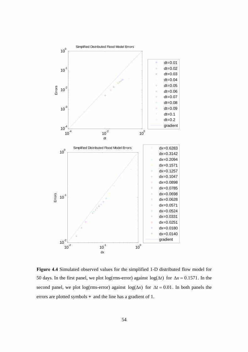
54

10-4 10-2 100

10-4

10-3

10-2

10-1

100

dt

Erro

rs

Simplif ied Distributed Flood Model Errors

dt=0.01dt=0.02dt=0.03dt=0.04dt=0.05dt=0.06dt=0.07dt=0.08dt=0.09dt=0.1dt=0.2gradient

10-2 10-1 100

10-2

10-1

100

dx

Erro

rs

Simplif ied Distributed Flood Model Errors

dx=0.6283dx=0.3142dx=0.2094dx=0.1571dx=0.1257dx=0.1047dx=0.0898dx=0.0785dx=0.0698dx=0.0628dx=0.0571dx=0.0524dx=0.0331dx=0.0251dx=0.0180dx=0.0140gradient

Figure 4.4 Simulated observed values for the simplified 1-D distributed flow model for

50 days. In the first panel, we plot log(rms-error) against )log( t∆ for 1571.0=∆x . In the

second panel, we plot log(rms-error) against )log( x∆ for 01.0=∆t . In both panels the

errors are plotted symbols ∗ and the line has a gradient of 1.

55

4.7 Summary

In this Chapter, we described our new simplified 1-D distributed flow model and its

numerical implementation. In the presentation of the methodology of the flood model

main point was the assumption of periodic boundary conditions (not very realistic). We

showed also that the numerical scheme (upwind scheme), which used to discretize the

simple kinematic wave equation (4.1) for our experiments in the MATLAB code, is first

order accurate in time and space, but suffers from numerical diffusion.

Particularly, the experiments in Section 4.6 have revealed one main feature, after

demonstrating the order of accuracy of the numerical scheme and showing the qualitative

behaviour of the numerical model with time and in space for several time steps. This

main feature states as: low order numerical schemes, such as the upwind scheme that

used in the experiments with the flow model, tend to have numerical diffusion. A useful

approach to manage with this problem is to be careful to have sufficiently many spatial

grid points, since after several runs of the flow model we observed better results for large

state space dimension. A higher order numerical method may be identified as an area for

further investigation. Finally, it is worth noting that the choice of space and time steps

plays also significant role for future Chapters, especially, for demonstrating the filter

behaviour in Chapters 5 and 6. Chapter 5 is about the implementation of an EnKF

algorithm, the ETKF, using the MATLAB code written for Livings, (2005), through

modifications and additions have been made for this thesis. The key idea is to modify

ETKF for use with rainfall inputs and the simplified 1-D distributed flow model. And in

Chapter 6 we give the experimental results of the implemented ETKF.

We concluded also that the method suffers from some arbitrary choices. These include

the choice of the parameter a (a parameter in the simple flow model that we chose to

depend on soil, geology, land cover etc.). Parameter, space and time limitations can result

in the accuracy of the distributed flood model but we still can have good results, as we

observed. Finally, the experiments have revealed that for numerical stability ‘safe’ ranges

for the dimensionless wave speed θ are between zero and one.

56

Chapter 5

Implementing an Ensemble Kalman Filter

In this Chapter we describe the implementation of an EnKF; the Ensemble Transform

Kalman Filter (ETKF). We present, also, a new modification of the ETKF for use with

(rainfall) inputs and a simple flood model.

5.1 Implementing the ETKF

In Section 3.6 we gave a description of the ETKF algorithm, but in this Section we

describe the Livings, (2005) unbiased implementation of the ETKF. It is worth noting

that the eigenvalue decomposition, equation (3.26)

UΛYRY =− fTf 1)( TU ,

produced eigenvalues and eigenvectors with significant imaginary parts in Livings,

(2005) first implementation. Livings, (2005) found a way to avoid these problems by

developing a new implementation. The new implementation introduces a scaled forecast

observation ensemble perturbation matrix,

ff YRY 21

ˆ −= . (5.1)

Hence, from the above relationship, equation (3.26) becomes

57

fTffTf YYYRY ˆ)ˆ()( 1 =− . (5.2)

Using the Singular Value Decomposition (SVD) by Livings, (2005) we have that

TTf VUΣY =)ˆ( , (5.3)

where U is the )( NN × orthogonal matrix, Σ is the )( pN × diagonal matrix and V is

the )( pp× orthogonal matrix. Note that U matrix in equation (5.3) is in fact the same

U matrix in equation (3.26). The singular value matrix, Σ , and the diagonal matrix of

eigenvalues, Λ , are related by TΣΣΛ = .

The updated ensemble perturbation matrix is then

TXX fa =

TTf UΣΣIUX 21

)(−

+= . (5.4)

This choice of matrix T ensures that the filter is unbiased in the sense of Livings et al.,

(2008). Using equation (3.17) and the SVD (5.3) we conclude to the following expression

of the Kalman gain

1))(()( −+= RYYYXK TffTffe

21

1))ˆ(ˆ()ˆ(−−+= RIYYYX TffTff

21

1)(−−+= RVIΣΣUΣX TTf . (5.5)

Finally, instead of computing the Kalman gain eK and then the ensemble mean

)( fe

fa yyKxx −+= , it is better to build up the product

)()( 21

1 fTT yyRVIΣΣΣz −+=−− (5.6)

58

from right to left and then update the ensemble mean by UzXxx ffa += . With this

process we avoid storing the Kalman gain eK and we only need to store a vector at each

stage of building up z (Livings, 2005).

The experimental results by implementing the ETKF algorithm in MATLAB are given

in detail in Chapter 6. Note that the SVD (5.3) is performed using the standard MATLAB

svd function which uses the LAPACK routine DGESVD (Anderson et al., 1999).

5.2 Implementing the ETKF for use with inputs

In Chapter 3 (Section 3.6) and in Section 5.1 we gave an analytic description of the

ETKF algorithm that we will use in our research. However, we have not yet considered

how to deal with the precipitation inputs. For this case, the true state of the system at time

kt , satisfies

))(),(),(()( 111 −−−= kkkt

kt tttft ηuxx , (5.7)

where f is the function that relates the state at the previous time step 1−k to the state at

the time step k . This function in our research is given by the finite difference scheme

(4.16) we used to discretize the simple kinematic wave equation (4.1) of the simple flow

model (implemented in Chapter 4). Finally, this function includes as parameters any

function of the (rainfall) input u and any function of the model noise η at the previous

time step 1−k .

In Section 3.3.1 we gave an analytic description of the Kalman Filter algorithm that deal

with rainfall inputs. Hence, using these equations from Section 3.3.1, the analogous

equations for the ETKF are given as follows by assuming two different cases for the

precipitation inputs.

59

Case 1: Rainfall input u is perfectly known.

In this case there is only one input u and the only change to the algorithm described in

Section 3.3.1 is to take account of the inputs in the forecast step as in equation (3.3).

Considering a nonlinear dynamical model M in the state forecast step the ensemble is

propagated forward in time using the following nonlinear model:

)()())(()( 111 −−− ++= kikkaik

fi tttMt ηNuxx , (5.8)

for Ni ≤≤1 . In this relationship )( kfi tx represents the ith ensemble forecasted state at

time kt , )( 1−kai tx is the ith updated ensemble state at the previous time 1−kt , )( 1−ktu is the

precipitation input at the previous time 1−kt and )( 1−ki tη is a Gaussian pseudo-random

model noise at the previous time 1−kt which for our implementation we assume that is

equal to zero. Matrix N , in equation (5.8), is defined based on knowledge of the process

given in Section 3.3.1. Note that a more complex (nonlinear) relationship between the

state and input u is possible, and could be dealt with in the same way. The case

described here is the case we have done our experiments on.

Then, the ensemble mean, the ensemble perturbation matrix and the ensemble

covariance matrix are given by equations (3.12), (3.13) and (3.14) from Section 3.4.2. We

assume, after, as in Section 3.4.3 an observation y of dimension p , and an observation

operator H (possibly nonlinear) which maps the state vector to the observation vector.

We introduce an ensemble of forecast observation ))(()( kfik

fi tHt xy = , where )( k

fi ty

represents that observation if )( kfi tx is the true state of the system at time kt without

observation noise, for Ni ≤≤1 (Livings et al., 2008). For the case of imperfect

observations we give an ensemble of forecast observation )())(()( kikfik

fi ttHt εxy += ,

where )( ki tε is a Gaussian, random, unbiased and uncorrelated observation noise at the

same time kt with mean zero and known covariance matrix R . Then we follow the

procedure described in Section 5.1, where instead of computing the Kalman gain eK and

then the ensemble mean (3.21), it is better to build up the product (5.6) from right to left

60

and then update the ensemble mean by UzXxx ffa += . The above equations can be

generalized for both linear and nonlinear observation operators (Livings et al., 2008).

Case 2: Rainfall input u is uncertain and can be treated as a random variable.

In this case we may have an ensemble of inputs, so we can obtain for the forecast step

)()())(()( 111 −−− ++= kikikaik

fi tttMt ηNuxx , (5.9)

where )( 1−ki tu is the rainfall input of the ith ensemble member at the previous time 1−kt .

Then, the procedure is similar to the one described above but the difference pointed to the

calculation of the forecast error covariance matrix fP , equation (3.4). Assuming that we

have input errors, we calculate the forecast error covariance matrix including these errors.

Something similar was done in the Srikanthan et al., (2007) but for the perturbed

observation filter where in addition to representing the noise )( 1−ki tη with zero mean and

know covariance matrix Q , this EnKF represents the multiplicative model errors through

forcing data perturbations. The input data perturbations are made by adding the Gaussian

noise )( ki tζ with mean zero and known covariance matrix to the rainfall input data at

each time step: )()()( kikki ttt ζuu += . (5.10)

Finally, as mentioned before, for our experiments in Chapter 6 we just use single

(rainfall) inputs which specified a priori as we did in the implemented simplified 1-D

distributed flow model. Hence, the possibility of working as described above with an

ensemble of inputs may be an area for further investigation. The assumption also of

treating rainfall input u as a Gaussian or non-Gaussian variable would be an interesting

work.

61

5.3 Summary

The purpose of this Chapter was to provide a presentation of the ETKF algorithm

implementation. We started in Section 5.1 with a brief description of the unbiased ETKF

algorithm as a solution to avoid problems we faced with the eigenvalue decomposition in

Chapter 3, with main point the use of the Singular Value Decomposition (SVD) which is

performed in our experiments using the standard MATLAB svd function. Later, in

Section 5.2 we discussed new ideas for use of (precipitation) inputs with the ETKF,

focusing in two cases. For the first case we considered that rainfall inputs are perfectly

known single inputs and in the second case that are random variables (e.g. ensemble of

inputs).

In Chapter 6 we present experimental results using our filter implementation with the

simplified flood model of Chapter 4.

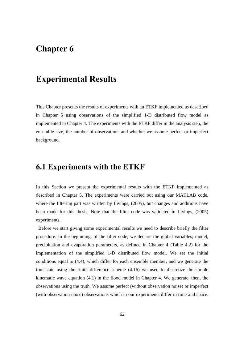
62

Chapter 6

Experimental Results

This Chapter presents the results of experiments with an ETKF implemented as described

in Chapter 5 using observations of the simplified 1-D distributed flow model as

implemented in Chapter 4. The experiments with the ETKF differ in the analysis step, the

ensemble size, the number of observations and whether we assume perfect or imperfect

background.

6.1 Experiments with the ETKF

In this Section we present the experimental results with the ETKF implemented as

described in Chapter 5. The experiments were carried out using our MATLAB code,

where the filtering part was written by Livings, (2005), but changes and additions have

been made for this thesis. Note that the filter code was validated in Livings, (2005)

experiments.

Before we start giving some experimental results we need to describe briefly the filter

procedure. In the beginning, of the filter code, we declare the global variables; model,

precipitation and evaporation parameters, as defined in Chapter 4 (Table 4.2) for the

implementation of the simplified 1-D distributed flow model. We set the initial

conditions equal to (4.4), which differ for each ensemble member, and we generate the

true state using the finite difference scheme (4.16) we used to discretize the simple

kinematic wave equation (4.1) in the flood model in Chapter 4. We generate, then, the

observations using the truth. We assume perfect (without observation noise) or imperfect

(with observation noise) observations which in our experiments differ in time and space.

63

Particularly, we run the filter code assuming imperfect observations and we generate the

ensemble of observations at each update time by giving noise with zero mean and

covariance equal to the observation error covariance matrix R . An initial ensemble of

state estimates is then chosen. This ensemble of vectors is drawn from a normal

distribution with a given covariance matrix and the true initial state. We assume in our

experiments perfect or imperfect background, where for the first case the ensemble is

translated so that the ensemble mean coincides exactly with the true initial state. These

sample points are then propagated through the system. The approximation of forecast

state error covariance matrix is made by propagating the ensemble of model states using

the updated state from the previous time step. Note that there is no model noise in the

ensemble forecasts as well as in the truth forecast. Finally, we have to mention that

rainfall inputs (single inputs) and evaporation are specified a priori inside the flow model.

Figures 6.1 and 6.2 show the experimental results by running the ETKF for 10 days over

0.01-time interval and a state space of dimension n =150 (this choice ameliorates

numerical diffusion in the model, see Section 4.6). The main point of these figures is to

compare the results, if we assume that the estimates are derived with the ETKF using

ensemble members 4=N and we run the ETKF for different number of imperfect

observations over time. The ensemble size is rather small, although that is more like

operations. Examples assuming ensemble size 27=N are given in Appendix B.

Specifically, in figures 6.1 and 6.2 we give a sequence of plots where in each graph we

simulate 1, 5, 10 and 20 distinct measurements (imperfect observations) that have errors

normally distributed around zero with standard deviation 1.0; in figure 6.1 we assume

perfect background and in figure 6.2 imperfect. All coordinates are observed in space but

in the 1st panel of figures observation is taken at the last time grid point (the last day), in

the 2nd panel the measurements are taken every 200 time steps, in the 3rd panel of figures

every 100 time steps and finally in the 4th panel observations are taken every 50 time

steps up to the 10th day. Figures 6.1 and 6.2, generally, illustrate the difference between

the filter and the truth. Specifically, each panel in these figures represents the first

component of the output of the ETKF plotted relative to the truth. The value of the true

state is indicated by the dotted line at zero. The three solid lines show ensemble mean

(red line) and ensemble mean ± ensemble standard deviation. Finally, in each panel the

64

first component of assimilated observations are given as + with error bars indicating the

observation standard deviation.

All graphs in figure 6.1 start with the same ensemble and show the expected result, filter

convergence by taking more observations over time. Comparing the panels in figure 6.1

we observe that if more observations are assimilated, during the 10 days we run the

ETKF, the true state is often inside the band given by the ensemble mean ± ensemble

standard deviation, indicating that the filter has stable behaviour. It should also be noted

that the excellent estimates obtained in our experiment reflect the fact that we assume

perfect background which indicate positions that start from the ‘correct’ point, and the

fact that the model used in the forecast step is the same as the model used to generate the

truth. In the first panel of this figure, when no observations are assimilated, we observe

divergent and convergent behaviour (just after the 2nd and 8th day) of the ensemble spread

(indicated by ± ensemble standard deviation). Specifically, by plotting the ensemble

members (for the first panel when no observations are assimilated; plots are not shown)

we observe that the ensemble members have different frequency of oscillation about the

true trajectory. That might happen, since the initial conditions differ for each ensemble

member and precipitation, evaporation play a significant role in the filter (affect solution

behaviour). As it concerns the behaviour of the ensemble standard deviation in the last

three panels of both figures, we are able to observe that become smaller after the first

observation. It is worth noting that the observation variance is specified a priori and it

remains fixed through the experiments. We conclude, thus, that we observed better

results for more measurements over time, since the filter taking notice of observations.

That indicates stable filter behaviour, but the possibility of generalizing the experimental

results may lead to errors for reasons that are given in detail later in this Section.

In figure 6.2, as mentioned before, we assume imperfect background (position that starts

from ‘wrong’ point). That affects, as we expected, the filter behaviour. All the panels

(especially the first three) in this figure indicate the fact that the true state is often outside

the band given by the ensemble mean ± ensemble standard deviation. It is clear also,

especially in the last three panels, that the ensemble spread is too small. We expected to

observe that results, since we work with a random sampling problem, where sometimes

the samples do not lie within the band given by the ensemble mean ± ensemble standard

65

deviation. Note, finally, that the choice of the ensemble size play significant role and we

have to point out that for larger number of ensemble members we observe ‘better’ results.

These are illustrated in Appendix B.

Generally, the use of small ensemble sizes often leads to less accurate results (Livings et

al., 2008). It is useful to consider how the ETKF estimates converge to the true state as

the ensemble size increases. Hence, for that purposes, figure 6.3 illustrates individual

ensemble members with the assumption of imperfect observations. For the experimental

results in figure 6.3 we run the ETKF for 10 days over 0.01-time interval and a state

space of dimension n =150, since for small number of space grid points we face problems

(numerical diffusion) with the implemented flood model. Each panel of figure 6.3 is for

4, 10, 50 and 100 ensemble members respectively which are represented as red lines. In

these experiments, we observe all the components in space and we assume 20

measurements over time plotted as error bars of the 20th coordinate. In figure 6.3, we

assume perfect background and we use the same observations for each ensemble. The

case of imperfect background is illustrated in Appendix B. An important feature of the

these experimental results is the fact that the ensemble spread is getting smaller after the

first observation; and that is clear in all panels of figure 6.3. Finally, we are able to

observe that after the first couple of observations are assimilated, the ETKF estimates

converge to the true state, as we expected. That becomes more obvious when the

ensemble size is increased, as in the last three panels of figure 6.3.

It is very important to be mentioned that after several trials of the filter we chose again,

for all the experiments, to run the simplified 1-D distributed flow model and hence the

ETKF for value of parameter a equal to 0.05 (the parameter that was chosen in our

research to depend on soil, geology, land cover etc.). With that value we allow to rainfall

and evaporation to have the significant role in the filter, but at the same time we keep a

balance as it concerns the increasing values of river flow during the last experimental

days. Note that in Chapter 4, we made the assumption that is raining 20 times more than

we have evaporation. Hence, it was expected, by increasing the value of the parameter

(increasing also the forecast errors) to observe filter divergence and by decreasing the

value (decreasing the forecast errors) to obtain stable filter behaviour, whether we assume

perfect or imperfect background (the plots are not shown).

66

0 2 4 6 8 10 12-2

-1

0

1

time (Days)

z 1 - z 1t

0 2 4 6 8 10 12-2

0

2

4

time (Days)

z 1 - z 1t

0 2 4 6 8 10 12-2

0

2

4

time (Days)

z 1 - z 1t

0 2 4 6 8 10 12-4

-2

0

2

4

time (Days)

z 1 - z 1t

Figure 6.1 Imperfect observations, perfect background. The 1st, 2nd, 3rd and 4th panel

show the first component of the output of the ETKF plotted relative to the truth for

number of observations 1, 5, 10 and 20 over time, respectively. Ensemble size is taken

equal to 4=N .

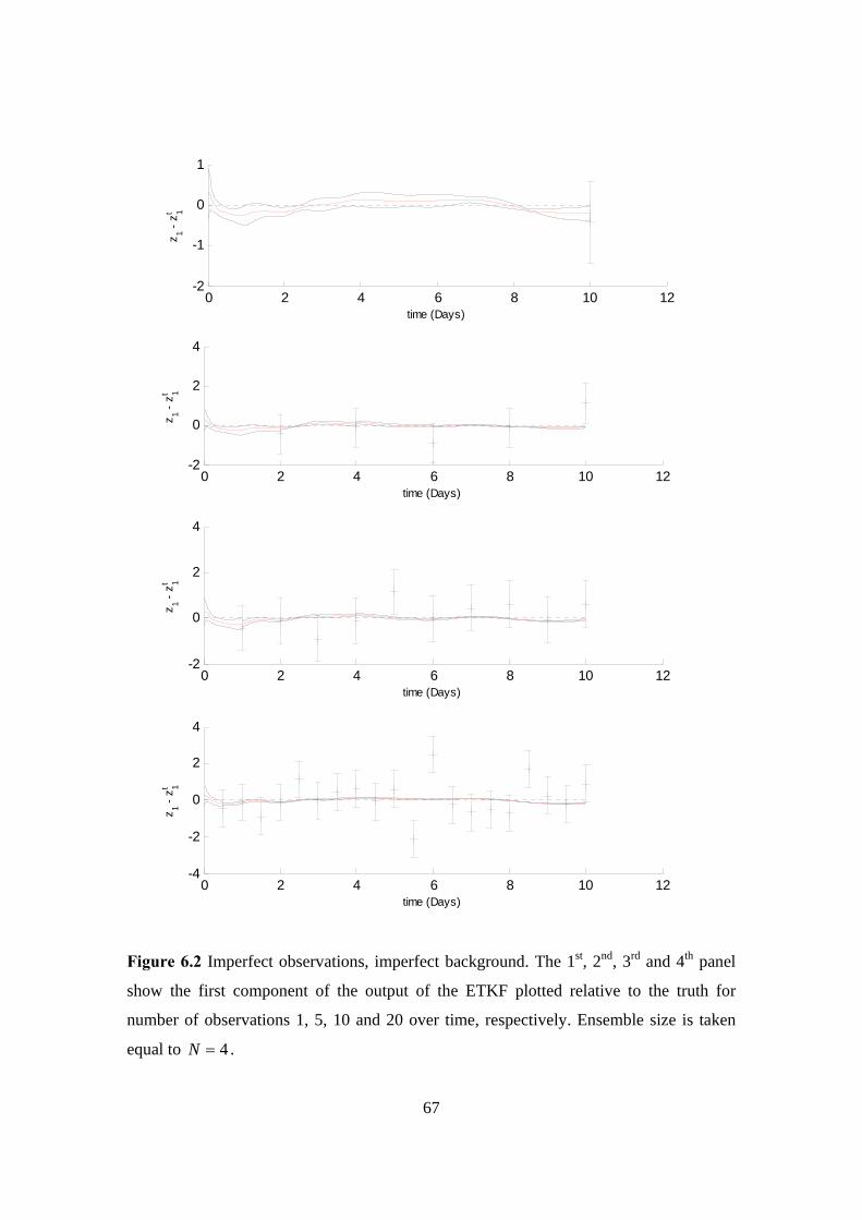
67

0 2 4 6 8 10 12

-2

-1

0

1

time (Days)

z 1 - z 1t

0 2 4 6 8 10 12-2

0

2

4

time (Days)

z 1 - z 1t

0 2 4 6 8 10 12-2

0

2

4

time (Days)

z 1 - z 1t

0 2 4 6 8 10 12-4

-2

0

2

4

time (Days)

z 1 - z 1t

Figure 6.2 Imperfect observations, imperfect background. The 1st, 2nd, 3rd and 4th panel

show the first component of the output of the ETKF plotted relative to the truth for

number of observations 1, 5, 10 and 20 over time, respectively. Ensemble size is taken

equal to 4=N .

68

0 2 4 6 8 10 12-4

-2

0

2

4

time (Days)

x 20-x

t 20

0 2 4 6 8 10 12-4

-2

0

2

4

time (Days)

x 20-x

t 20

0 2 4 6 8 10 12-4

-2

0

2

4

time (Days)

x 20-x

t 20

0 2 4 6 8 10 12-4

-2

0

2

4

time (Days)

x 20-x

t 20

Figure 6.3 ETKF, perfect background, N = 4, 10, 50 and 100 the ensemble members for

the 1st, 2nd, 3rd and 4th panel, respectively. Red lines show individual ensemble members

and the imperfect observations are plotted as error bars.

69

So far we show the behaviour of the filter if we observe all the components in space and

changing the assimilated observations in time. It is worth presenting the experimental

results by keeping the number of imperfect observations stable over time (20

measurements in time) and changing the number of observations in space. In the

following figures 6.4 and 6.5, we present a sequence of plots by assuming that we

observe 1, 15 and 50 components in space (panels in figures 6.4 and 6.5 are with the

same sequence). In the first case we observe only the first component, in the second case

we observe every 10 grid points and in the last case every 3. For the following

experimental results we run the ETKF for 10 days over 0.01-time interval and a state

space of dimension n =150. Also, we assume perfect background and size of ensemble

members 27=N . The experimental results, in figure 6.4, illustrated by giving the first

component of the output of the ETKF of an observed grid point plotted relative to the

truth and in figure 6.5 of an unobserved grid point. Note that the assimilation is able to

adjust the unobserved components towards the truth even though they are not observed.

The dotted line at zero represents the true state. The red line represents the ensemble

mean and the other two lines indicate ensemble mean ± ensemble standard deviation.

It is worth noting, if we compare these two figures, that the filter behaviour is different

for the observed and unobserved points, as we expected. Since, these figures represent the

difference between the filter and the truth we are able to obtain, in figure 6.4 that the true

state is inside the band defined by the ensemble mean ± ensemble standard deviation,

especially in the last panel, where more observations are used. Also, it is important to be

mentioned for the same figure that the size of the ensemble spread is getting smaller as

we take more measurements. Finally, in the second panel of figure 6.4, though the small

number of the assimilated observations, a further consequence may be unstable filter

behaviour in comparison with the last panel where the filter converges. On the other

hand, in figure 6.5 the true state is often outside the band defined by the ensemble mean

± ensemble standard deviation in the third panel, but in the other two is inside. That

might happen because the filter gives more weight than it should to the forecast in the

next analysis step and less to the observation. Note also that the problem is a random

sampling problem and thus we expected these experimental results.

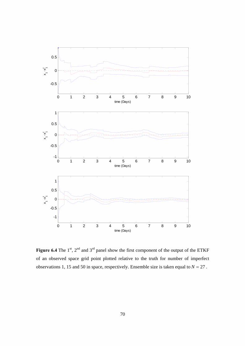
70

0 1 2 3 4 5 6 7 8 9 10

-0.5

0

0.5

time (Days)

x 1 -x1t

0 1 2 3 4 5 6 7 8 9 10-1

-0.5

0

0.5

1

time (Days)

x 1 -x1t

0 1 2 3 4 5 6 7 8 9 10

-1

-0.5

0

0.5

1

time (Days)

x 1 -x1t

Figure 6.4 The 1st, 2nd and 3rd panel show the first component of the output of the ETKF

of an observed space grid point plotted relative to the truth for number of imperfect

observations 1, 15 and 50 in space, respectively. Ensemble size is taken equal to 27=N .

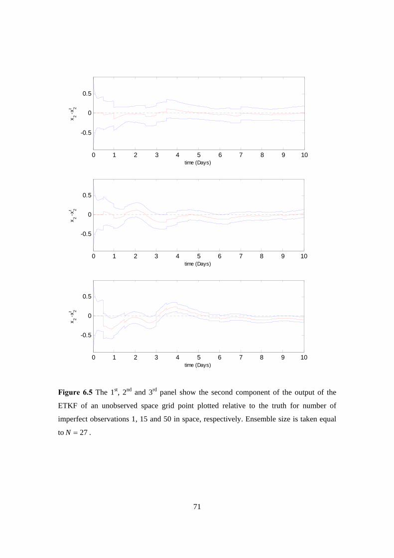
71

0 1 2 3 4 5 6 7 8 9 10

-0.5

0

0.5

time (Days)

x 2 -x2t

0 1 2 3 4 5 6 7 8 9 10

-0.5

0

0.5

time (Days)

x 2 -x2t

0 1 2 3 4 5 6 7 8 9 10

-0.5

0

0.5

time (Days)

x 2 -x2t

Figure 6.5 The 1st, 2nd and 3rd panel show the second component of the output of the

ETKF of an unobserved space grid point plotted relative to the truth for number of

imperfect observations 1, 15 and 50 in space, respectively. Ensemble size is taken equal

to 27=N .

72

The ETKF has been performed within contexts of the simplified 1-D distributed flow

model, which is a low dimensional model and offers the obvious advantage of a much

reduced dimensionality n of the state vector x (in terms of calculations in the

implemented filter). In this implementation of the ETKF we make use of a state space of

dimension 150=n (such a small number), for computational reasons. This is an

important limitation as reviewed in Ehrendorfer, (2007) and the possibility of

generalizing the experimental results may lead to errors, in terms of filter divergence or

convergence. In our research we obtained stable filter behaviour (filter convergence).

Also, the sequential nature of the ETKF may lead to filter convergence or to unphysical

stationary (same filter behaviour) results (Ehrendorfer, 2007). The nature of the

stationary properties of the KF and EnKF has been considered in detail by Daley and

Menard, (1993) and Ehrendorfer, (2007), but in our research we did not face problem

with stationary filter behaviour. Hence, in view of the above discussion and presentation

of the experimental results we expect that the assimilation results might be quite different

when obtained on the basis of a more active assimilation model. Such a model will be if

we increase the dimension of the state space, the number of days (that we run the model)

and the size of ensemble members. Thus, we need to take into account the above issues,

when trying to explain the experimental results and the filter behaviour. Although, the

carefully usage of the simplified distributed flow model offers advantages and should be

considered useful for assimilation methods, especially with EnKF methods.

6.2 Summary

In this Chapter we represented the experimental results with an Ensemble Square Root

Filter; the implemented Ensemble Transform Kalman Filter (ETKF), of Chapter 5, in

conjunction with the simplified 1-D distributed flow model of Chapter 4. The ETKF was

modified for use with single inputs which specified a priori in the filter. The possibility to

deal with random inputs (e.g. an ensemble of inputs) requires further investigation. One

of the purposes of this thesis was to investigate the effects of ensemble size and

73

observation frequency on the behaviour of the forecast-assimilation dynamical system.

Hence, it is important to be mentioned that the use of small ensemble sizes often led to

less accurate results, since we observed that the ETKF estimates converge to the true

state as the ensemble size increases. It was clear also, from the experiments, the fact that

if more observations were assimilated, during the days we run the filter, the true state was

often inside the band defined by the ensemble mean ± ensemble standard deviation,

indicating filter convergence. Moreover, the experiments have revealed and the following

main points. The first feature pointed in the fact that the choice of perfect or imperfect

background may affect the filter behaviour. The selection of perfect background usually

led in stable filter behaviour and for the selection of imperfect background we had to take

into consideration the fact that the problem was a random sampling problem, where

sometimes the samples do not lie within the band of ensemble mean ± ensemble

standard deviation. The second feature was the fact that although we observed stable

filter behaviour, the usage of the simplified low-dimensional (1-D) distributed flow

model and the sequential nature of the ETKF may lead to this filter convergence. Finally,

the choice of the values of parameter a which controls the behaviour of the rainfall

inputs in our research may lead to different results than the one we observed. However,

parameter, space, time, ensemble size and background limitations can result in the

accuracy of the filter but we still can have good results.

74

Chapter 7

Conclusions

7.1 Summary and Discussion

The purposes of this dissertation were to design and implement a simplified one

dimensional (1-D) distributed flow model, using a similar to the Grid-to-Grid routing

scheme (Moore et al., 2006) and to modify an Ensemble Kalman Filter (EnKF), the

Ensemble Transform Kalman Filter (ETKF), for use with (rainfall) inputs and the

simplified 1-D distributed flow model.

In Chapter 2, we introduced an overview of flood forecast models, focusing on the

distributed Grid-to-Grid flow model (Moore et al., 2006), and we represented briefly the

sources of uncertainty in flood modelling which divided in three categories by Leahy et

al., (2007): input uncertainty of rainfall, model uncertainty and output uncertainty. An

ensemble approach has been developed to try and deal with rainfall uncertainty, by using

ensemble rainfall forecasts as an input to an ensemble flood model. It seems natural to

combine this approach with an ensemble data assimilation system and these ideas were

discussed in Chapter 3.

Our fundamental issue in Chapter 3 related to the description of data assimilation

techniques, such as the Kalman (presented in Welch & Bishop, 2006) and Ensemble

Kalman Filter methods which are valuable in flood forecasting. The Kalman Filter (KF)

developed for linear dynamic systems and provided a means of explicitly taking account

of input, model and output uncertainties. For nonlinear dynamic systems EnKF

techniques (presented in Evensen, 2003) provided an alternative method of estimating

these uncertainties by the use of an ensemble of state estimates instead of a single state

estimate and without maintaining a separate error covariance matrix. These data

75

assimilation methods are useful in flood forecasting, since the use of real-time flood

models requires attention to uncertainty estimation and model initialization (i.e. state

estimation); problems which can be solved using these techniques. It is important to be

mentioned, that the EnKF was not originally designed to take into account (rainfall)

inputs and hence the algorithms described without that assumption.

In Chapter 4, the key idea was to introduce a new simplified 1-D distributed flood

model, as a subject for experiments, assuming periodic boundary conditions. The

assumption of periodic boundary conditions was not very realistic, since few rivers have

a loop shape. However, we have chosen these conditions to make our flow model easier

to implement numerically. We gave an analytic description of the flow model

methodology; focusing on the numerical scheme (upwind scheme which is first order

accurate in time and space) we chose to integrate the simple kinematic wave equation

(4.1). The experimental results, of the simplified 1-D distributed flow model, show that

low order numerical schemes, such as the upwind scheme tend to have numerical

diffusion. A useful approach to manage with this problem was to be careful to have

sufficiently many spatial grid points, since after several runs of the flow model we

observed better results for large state space dimension. We concluded also that the

method suffers from some arbitrary choices. These include the choice of the parameter a

(a parameter in the simple flow model that we chose to depend on soil, geology, land

cover etc.). Moreover, an important limitation of our research was that we have used

prescribed functions for precipitation and evaporation inputs and not any real data to

compare our flow model performance with reality. However, the character of the partial

differential equation (PDE) we chose to solve (hyperbolic with forcing) is similar to that

used in more realistic models such as the Grid-to-Grid model by Moore et al., (2006),

where the several trials of this model on simply responding catchments could help us

understand how easily and widely the simplified distributed flood model could also be

applied to address the ungauged forecasting problem at any location within a chosen

domain. Hence, parameter, space and time limitations can result in the accuracy of the

distributed flood model and in the applicability of our work but we still can have good

results, and the approach we described in this thesis is a sensible way forward for

research.

76

Chapter 5 was about the presentation of an implemented EnKF; the ETKF using the

MATLAB code written for Livings, (2005), through modifications and additions have

been made for this thesis. The purpose of this Chapter was to provide a complete

interpretation of the ETKF and to present new ideas that used in the implemented ETKF.

The key idea was to modify the ETKF for use with inputs and a simple flood model, as

described in Chapter 4. For our implementation we used single inputs and the possibility

of working with an ensemble of inputs may be an area for further investigation.

Finally, in Chapter 6 we gave an analytic presentation of the experimental results using

the ETKF implementation of Chapter 5. We gave explanations of the features we

observed from the experiments and of the problems that were encountered with the

implemented ETKF. We observed that the filter behaviour depends on the assumption of

perfect or imperfect background and on the size of ensemble members. The selection, in

our experiments, of perfect background usually led in stable filter behaviour. And the use

of small ensemble sizes often led to less accurate results, since we observed that the

ETKF estimates converge to the true state as the ensemble size increases. The

experiments revealed also the following main point. From the ETKF experiments we

observed stable filter behaviour, but the usage of the simplified low-dimensional (1-D)

distributed flow model and the sequential nature of the ETKF may led to this filter

convergence. Hence, in view of the experimental results in Chapter 6, we expect that the

assimilation results might be quite different when obtained on the basis of a more active

assimilation model. Such a model will be if we increase the dimension of the state space,

the number of days and the size of ensemble members. The filter, also, may suffer from

some arbitrary choices such as the choice of the parameter a (a parameter in the simple

flow model that we chose to depend on soil, geology, land cover etc. and controls the

behaviour of rainfall inputs). The assumption of taking the model error equal to zero in

the filter, the fact that we chose not applying the usual covariance inflation and

localization that is common in EnKF usage and the use of a square root filter rather than a

perturbed observation filter may limit also the applicability of our work, but, although

these limitations, this filter is a sensible way forward for research and operations.

77

7.2 Further work

Three main areas may be identified for further investigation, as it concern the

implementation of the simplified 1-D distributed flow model (Chapter 4) and the

implemented ETKF (Chapter 5): the numerical scheme used to integrate the simple

kinematic wave equation of the simplified 1-D distributed flood model, the assumption of

no spatially uniform model parameters and the assumption of random (rainfall) inputs.

• A higher order numerical method, instead of the upwind scheme (first order

accurate in time and space) used for the purposes of this thesis, may be identified

as an area for further investigation in the terms of discretize the simple kinematic

wave equation (4.1) in Chapter 4. The aforementioned numerical scheme tends to

have numerical diffusion.

• Precipitation, evaporation and routing parameters are considered to be spatially

uniform over the area corresponded to a channel plane. Hence, an area for further

investigation may be the assumption to vary these parameters from plane to plane.

• Implementation of the ETKF for use with random inputs (e.g. an ensemble of

inputs as described in Chapter 5) instead of single inputs which specified a priori

in our ETKF experiments may be identified as an area for further investigation.

For the case we have an ensemble of inputs, a realistic assumption about the

distribution of the precipitation will be the assumption of non-Gaussian rain, since

rainfall can not have negative values. However, something similar was presented

in the Srikanthan et al., (2007) paper for the perturbed observation filter, where

Gaussian rain used. Hence, it would be an interesting work to use log-normal

inputs and try to correct them using further observations, perhaps by smoothing

rather than filtering.

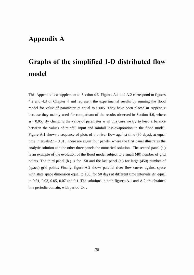
78

Appendix A

Graphs of the simplified 1-D distributed flow

model This Appendix is a supplement to Section 4.6. Figures A.1 and A.2 correspond to figures

4.2 and 4.3 of Chapter 4 and represent the experimental results by running the flood

model for value of parameter a equal to 0.005. They have been placed in Appendix

because they mainly used for comparison of the results observed in Section 4.6, where

05.0=a . By changing the value of parameter a in this case we try to keep a balance

between the values of rainfall input and rainfall loss-evaporation in the flood model.

Figure A.1 shows a sequence of plots of the river flow against time (80 days), at equal

time intervals 01.0=∆t . There are again four panels, where the first panel illustrates the

analytic solution and the other three panels the numerical solution. The second panel (a.)

is an example of the evolution of the flood model subject to a small (40) number of grid

points. The third panel (b.) is for 150 and the last panel (c.) for large (450) number of

(space) grid points. Finally, figure A.2 shows parallel river flow curves against space

with state space dimension equal to 100, for 50 days at different time intervals t∆ equal

to 0.01, 0.03, 0.05, 0.07 and 0.1. The solutions in both figures A.1 and A.2 are obtained

in a periodic domain, with period π2 .

79

0 20 40 60 800

2

4

Time (Days)

Flow

Analytic solution

0 20 40 60 800

2

4

Time (Days)

Flow

a.Approximate solution

0 20 40 60 800

2

4

Time (Days)

Flow

b.Approximate solution

0 20 40 60 800

2

4

Time (Days)

Flow

c.Approximate solution

Figure A.1 A sequence of plots of river flow against time (80 days at equal time

intervals 01.0=∆t ) for different state space dimensions (40, 150 and 450 spatial grid

points) and 005.0=a . This corresponds to Figure 4.2.

1 2 3 4 5 6

0.5

1

1.5

2

Space

Flow

Simplif ied Distributed Flood Model

dt=0.01dt=0.03dt=0.05dt=0.07dt=0.1

Figure A.2 The model was run for time 50=t days at different time intervals t∆ equal

to 0.01, 0.03, 0.05, 0.07 and 0.1. In the figure are shown parallel river flow curves against

space with state space dimension equal to 100 and 005.0=a . This corresponds to Figure

4.3.

80

Appendix B

Graphs of the ETKF This Appendix is a supplement to Chapter 6. Figures B.1, B.2 and B.3 correspond to

figures 6.1, 6.2 and 6.3 of Chapter 6 and represent the experimental results by running the

ETKF for ensemble size 27=N for figures B.1 and B.2 and for imperfect background

for figure B.3. They have been placed in Appendix because they mainly used for

comparison of the results observed in Chapter 6. By increasing the ensemble size we

observed ‘better’ results; filter convergence for both assumptions of perfect and imperfect

background in figures B.1 and B.2. Assuming imperfect background in figure B.3 we

observed that after the fourth observation is assimilated, the ETKF estimates converge to

the true state. The ETKF was run making all the assumptions as in Chapter 6 for each

figure.

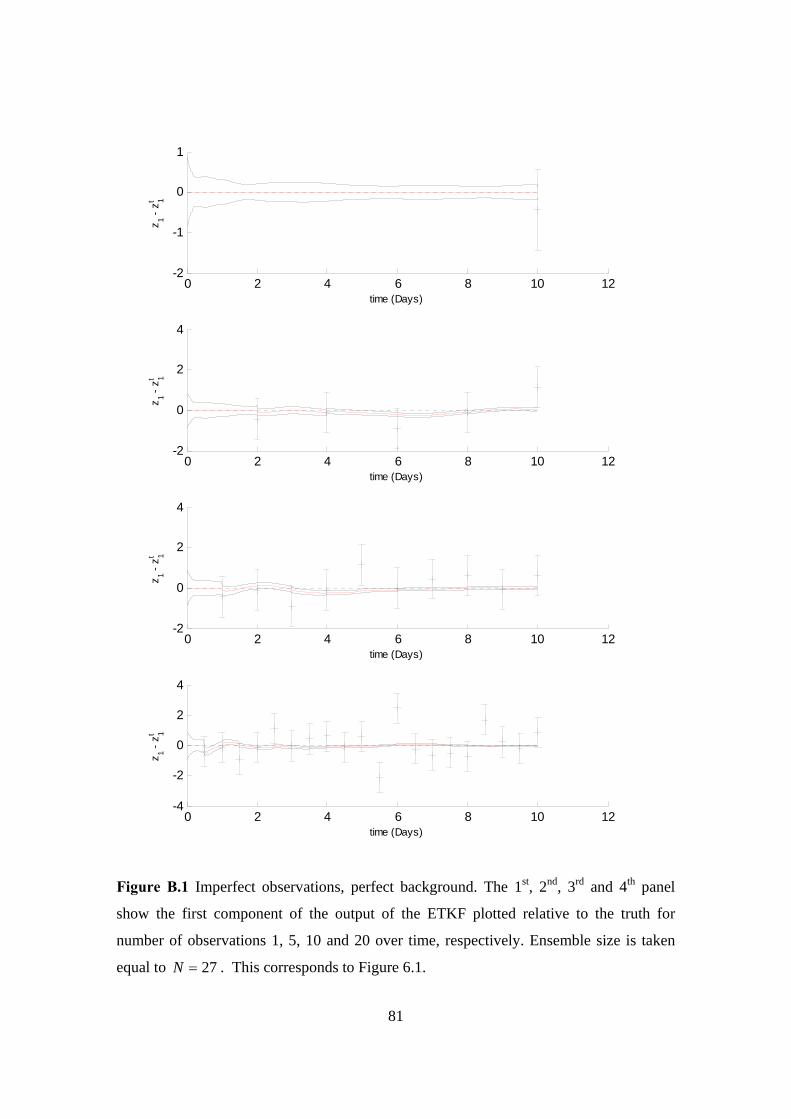
81

0 2 4 6 8 10 12-2

-1

0

1

time (Days)

z 1 - z 1t

0 2 4 6 8 10 12-2

0

2

4

time (Days)

z 1 - z 1t

0 2 4 6 8 10 12-2

0

2

4

time (Days)

z 1 - z 1t

0 2 4 6 8 10 12-4

-2

0

2

4

time (Days)

z 1 - z 1t

Figure B.1 Imperfect observations, perfect background. The 1st, 2nd, 3rd and 4th panel

show the first component of the output of the ETKF plotted relative to the truth for

number of observations 1, 5, 10 and 20 over time, respectively. Ensemble size is taken

equal to 27=N . This corresponds to Figure 6.1.

82

0 2 4 6 8 10 12-2

-1

0

1

time (Days)

z 1 - z 1t

0 2 4 6 8 10 12-2

0

2

4

time (Days)

z 1 - z 1t

0 2 4 6 8 10 12-2

0

2

4

time (Days)

z 1 - z 1t

0 2 4 6 8 10 12-4

-2

0

2

4

time (Days)

z 1 - z 1t

Figure B.2 Imperfect observations, imperfect background. The 1st, 2nd, 3rd and 4th panel

show the first component of the output of the ETKF plotted relative to the truth for

number of observations 1, 5, 10 and 20 over time, respectively. Ensemble size is taken

equal to 27=N . This corresponds to Figure 6.2.

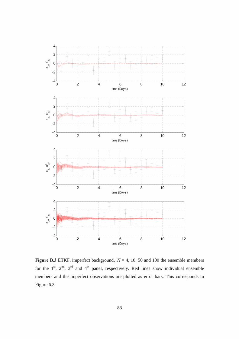
83

0 2 4 6 8 10 12-4

-2

0

2

4

time (Days)

x 20-x

t 20

0 2 4 6 8 10 12-4

-2

0

2

4

time (Days)

x 20-x

t 20

0 2 4 6 8 10 12-4

-2

0

2

4

time (Days)

x 20-x

t 20

0 2 4 6 8 10 12-4

-2

0

2

4

time (Days)

x 20-x

t 20

Figure B.3 ETKF, imperfect background, N = 4, 10, 50 and 100 the ensemble members

for the 1st, 2nd, 3rd and 4th panel, respectively. Red lines show individual ensemble

members and the imperfect observations are plotted as error bars. This corresponds to

Figure 6.3.

84

Bibliography Anderson, E., Bai, Z., Bischop, C., Blackford, S., Demmel, J., Dongarra, J., Du Croz, J.,

Greenbaum, A., Hammarling, S., McKenney, A. & Sorensen, D. (1999). LAPACK

User’s Guide. SIAM, 3rd Edition. Available from: www.netlib.org/lapack/lug

/lapack_lug.html.

Barlow, R. J. (1989). Statistics: A Guide to the Use of Statistical Methods in the Physical

Sciences, John Wiley & Sons Ltd., Chichester.

Bell, V. A., Kay, A. L., Jones, R. G. & Moore, R. J. (2007). Development of a high

resolution grid-based river flow model for use with regional climate model output.

Hydrology & Earth System Sciences, 11(1), 532-549.

Bishop, C. H., Etherton, B. J. & Majumdar, S. H. (2001). Adaptive sampling with the

ensemble transform Kalman Filter, part I: Theoretical aspects. Mon. Wea. Rev., 129,

420-436.

Daley, R. & Menard, R. (1993). Spectral characteristics of Kalman filter systems for

atmospheric data assimilation. Mon. Wea. Rev., 121, 1554 - 1565.

Dehotin, J. & Braud, I. (2008). Which spatial discretization for distributed hydrological

models? Proposition of a methodology and illustration for medium to large-scale

catchments. Hydrology & Earth System Sciences, 12, 769 - 796.

Ehrendorfer, M. (2007). A review of issues in ensemble-based Kalman filtering.

Meteorol. Z., 16(6), 795 - 818.

Evensen, G. (2003). The Ensemble Kalman Filter: Theoretical formulation and practical

implementation. Ocean Dynamics, 53, 343 - 367.

85

Gelb, A. (1974). Editor. Applied Optimal Estimation. The M.I.T. Press.

Kalnay, E. (2002). Atmospheric Modeling, Data Assimilation and Predictability.

Cambridge, UK: Cambridge University Press.

Koster, T., Sefary, G. E., Heemink, A. W., Boogaard, H. F. P. & Mynett, A. M. (2004).

Input correction in rainfall-runoff models using Ensemble Kalman Filtering (EnKF).

In: Lee, J. H. W. & Lam, K. M. (Eds.) Proc. 4th Int. Symp. On Environmental

Hydraulics, Hong Kong, 15-18 December 2004, Leiden Proc, Balkema, 1991 - 1996.

Available from: www.narcis.info/research/RecordID/OND1307340/Language

/en;jsessionid =knlq5muixm7 .

Leahy, C. P., Srikanthan, S., Amirthanathan, G. & Sooriyakumaran, S. (2007). Objective

Assessment and Communication of Uncertainty in Flood Warnings. 5th Flood

Management Conference Warrnamboll, 9-12 October 2007. 1- 6. Available from:

http://www.glenelg-hopkins.vic.gov.au/imageandfileuploads/Chris%20Leahy%20-

%20Objective%20Assessment%20and%20Communication%20of%20Uncertainty%2

0in%20Flood%20Warnings.doc.

Livings, D. (2005). Aspects of the Ensemble Kalman Filter. Master’s Thesis, University

of Reading, Reading, UK.

Livings, D. M., Dance, S. L. & Nichols, N. K. (2008). Unbiased ensemble square root

filters. School of Mathematics, Meteorology and Physics, University of Reading,

Reading, UK. ScienceDirect. Physica D, 237(8), 1021 - 1028.

May, B., Clark, P., Cooper, A., Forbes, R., Golding, B., Hand, W., Lean, H., Pierce, C.,

Roberts, N. & Smith, R. (2004). Numerical Weather Prediction: Flooding at Boscastle,

Cornwall on 16 August 2004 – A study of Met Office Forecasting Systems.

Forecasting Research Technical Report No.429. Met Office.

86

Michaud, J. & Sorooshian, S. (1994). Comparison of simple versus complex distributed

runoff models on a midsized semiarid watershed. Water Resources Research, 30(3),

593 -605.

Moore, R. J. (2007). The PDM rainfall-runoff model. Hydrology & Earth System

Sciences, 11(1), 483 - 499.

Moore, R. J., Bell, V. A. & Jones, D. A. (2005). Forecasting for flood warning. C. R.

Geoscience, 337, 203 - 217.

Moore, R. J., Cole, S. J., Bell, V. A. & Jones, D. A. (2006). Issues in flood forecasting:

ungauged basins extreme floods and uncertainty. Frontiers in Flood Research / Le

point de la recherché sur les crues, 305, 103 - 122.

Moore, R. J. & Weiss, G. (1980). Real-Time Parameter Estimation of a Nonlinear

Catchment Model Using Extended Kalman Filter. In: Wood, E. F. & Szollosi-Nagy,

A. Real- Time Forecasting/Control of Water Resource Systems. Pergamon Press, 83 -

92.

Morton, K. W. & Mayers, D. F. (2005). Numerical Solution of Partial Differential

Equations. Cambridge University Press.

Perry, C. A. (2000). Significant Floods in the United States during the 20th Century -

USGS Measures a Century of Floods. USGS science for a changing world. USGS

Fact Sheet 024-00 March 2000. Available from: http://ks.water.usgs.gov/Kansas/

pubs/fact-sheets/fs.024-00.html.

Pierce, C., Bowler, N., Seed, A., Jones, A., Jones, D. & Moore, R. (2005). Use of a

stochastic precipitation nowcast scheme for fluvial flood forecasting and warning.

Atmos. Science Letters, 6(1), 78 - 83.

87

Reed, S., Koren, V., Smith, M., Zhang, Z., Moreda, F., Seo, D. J. & DMIP Participants

(2004). Overall distributed model intercomparison project results. Journal of

Hydrology, 298(1-4), 27- 60.

Reichle, R. H., McLaughlin, D. B. & Entekhabi, D. (2002). Hydrologic Data

Assimilation with the Ensemble Kalman Filter. Monthly Weather Review. 2002, 130,

103-130.

Roberts, N. (2005). Numerical Weather Prediction: An investigation of the ability of a

storm scale configuration of the Met Office NWP model to predict flood-producing

rainfall. Forecasting Research Technical Report No. 455, Joint Centre for Mesoscale

Meteorology Report No. 150. Met Office.

Scott, A. S. (2003). The Method of Characteristics with applications to Conservation

Laws. Journal of Online Mathematics and its Applications (JOMA), 3, 1-11.

Srikanthan, R., Amirthanathan, G. E. & Kuczera, G. (2007). Application of Ensemble

Kalman Filter to Real-time Flood Forecasting. 2nd International Conference of GIS/RS

in Hydrology, Water Resources and Environment (ICGRHWE’ 07), Guangzhou,

China.

Tingsanchali, T. (1974). Forecasting model of Chao Phraya river flood levels at Bangkok.

The Chao Phraya Delta: Historical Development, Dynamics and Challenges of

Thailand’s Rice Bowl. International Conference of Chao Phraya Delta. Bangkok.

Thailand. 1 - 13. Available from: http://std.cpc.ku.ac.th/delta/conf/Acrobat/Papers

Eng/Volume%201/Tawatchai%20Paper%20OK.pdf

Tippett, M. K., Anderson, J. L., Bishop, C. H., Hamill, T. M. & Whitaker, J. S. (2003).

Ensemble square root filters. Mon. Weather Rev, 131, 1485 - 1490

88

Wang, X., Bishop, C. H. & Julier S. J. (2004). Which is better, an ensemble of positive-

negative pairs or a centered spherical simplex ensemble? Mon. Wea. Rev., 132, 1590 -

1605.

Welch, G. & Bishop, G. (2006). An Introduction to the Kalman Filter. Technical Report

No.95-041. Department of Computer Science, University of North Carolina at Chapel

Hill, Chapel Hill, NC 27599-3175. Available from: www.cs.unc.edu/~welch.

Wesseling, P. (1996). Von Neumann stability conditions for the convection-diffusion

equation. IMA Journal of Numerical Analysis, 16(4), 583 - 598.

Zappa, M., Rotach, M. W., Arpagaus, M., Dorninger, M., Hegg, C., Montani, A., Ranzi,

R., Ament, F., Germann, U., Grossi, G., Jaun, S., Rossa, A., Vogt, S., Walser, A.,

Wehrhan, J. & Wunram, C. (2008). MAP D-PHASE: real-time demonstration of

hydrological ensemble prediction systems. Atmospheric Science Letters, 9, 80 - 87.

89

Acknowledgments I would like to thank my supervisor Dr. Sarah Dance for her help and for continually

prodding me to make this thesis better. I wish I had the time to incorporate all her

valuable advices and suggestions.

Finally, I wish to thank the Department of Mathematics and Meteorology, University of

Reading for creating the course ‘Mathematical and Numerical Modelling of the

Atmosphere and Oceans’ and accepting me on it.

Declaration

I confirm that this is my own work, and the use of all material from other sources has

been properly and fully acknowledged.

Evangelia-Maria Giannakopoulou

.

90

.S. Geological Survey Kansas Water Science Center