R. & M. NoJ 3420

~'*~c~/,Fr JI,---

M I N I S T R Y OF A V I A T I O N

AERONAUTICAL RESEARCH COUNCIL

REPORTS AND MEMORANDA

Flight Measurements of the Drag of a Swept-Wing Aircraft (Hunter Mk. I)at Mach

Numbers up to 1.2, together with Some Measurements of Lift-Curve Slope

ByD. R. ANDREWS, B.Sc., B.Sc.(Eng.) and J. E. NETHAWAY, B .Sc.(Eng.)

LONDON: HER MAJESTY'S STATIONERY OFFICE

1966

PRICE IOS. 6 d . NET

Flight Measurements of the Drag of a Swept-Wing Aircraft (Hunter Mk. I ) a t Mach

Numbers up to i.~, together with Some Measurements of Lift-Curve Slope

ByD.R.ANDRews, B.Sc.,B.Sc.(Eng.) andJ. E.NerHAWA¥,B.Sc,(Eng.)

COMMUNICATED BY THE DIRECTOR-GENERAL OF SCIENTIFIC RESEARCH (AIR),

MINISTRY OF SUPPLY

Reports and Memoranda No. 3420*

June, ±955

Summary.

Flight tests have been made to determine the drag of a Hawker Hunter F Mk. I aircraft. The results show that at low Mach number the drag coefficient at zero lift is 0.0125 and the effective induced-drag factor K

is 1.09, both values being corrected to a constant Reynolds number of 34 x 10 G. Above a certain C L the drag

due to lift increases rapidly, the C L at which this occurs falling from 0.76 at M = 0.3 to 0.41 at M = 0" 7. Some approximate measurements of K made at supersonic speeds suggest that virtually all the leading-edge suction on the wing is lost beyond M = 1.0.

At C Z = 0-1, the compressibility drag rise commences soon after M -- 0.8, the drag rising rapidly beyond M = 0" 92 and attaining a peak C D of 0-0565 at M = 1-15. The compressibility drag rise obtained from high-speed wind-tunnel tests agrees well with that obtained in flight although this agreement may be largely fortuitous in view of the low tunnel Reynolds number.

Measurements of incidence show that the lift-curve slope at M = 0.3 is 3-5 rising to 4.6 at M = 0-9.

The zero-lift angle remains constant with Mach number at about 0-4 °. Agreement with wind-tunnel tests is reasonably good when allowance is made for differences in geometry and in Reynolds number.

,Section

1.

2.

3.

L I S T O F C O N T E N T S

In t roduc t i on

Details of Aircraft and In s t rumen ta t i on

M e t h o d of Tes t and Analysis of Results

3.1 D r a g Measu remen t s

3.1.1 Stabil ised Levels

3.1.2 Dives and Partial Glides

3.1.3 Accelerated and Decelera ted Levels

3.2 Correct ions to Fl ight Data

e Replaces A.R.C. 17 947.

Section

4.

LIST OF C O N T E N T S - - c o n t i n u e d

Results

4.1

4.2

4.3

and Discussion

Transition and Surface Roughness 4.1.1 Transition 4.1.2 Surface Roughness

Incidence and Lift-Curve Slope

Drag 4.3.1 4.3.2 4.3.3 4.3.4

Drag due to Lift Drag at CL'S of 0 and 0- 1 Accelerated and Decelerated Levels Comparison of Flight and Wind-Tunnel Results

4.4 Level-Flight Performance

5. Conclusions

Notation

References

Appendix--Effects of errors in incidence on the accuracy of drag measurements using the accelerometer technique

Table 1--Details of Hunter WT.571

Illustrations--Figs. 1 to 14

Detachable Abstract Cards

Figure

1.

2.

3.

4a.

4b.

5.

6a.

6b.

7.

8.

9.

10.

LIST OF I L L U S T R A T I O N S

General arrangement of Hawker Hunter F. Mk. I (WT.571)

General view of Hunter WT.571

Lift carpet ~or aircraft trimmed at 0.27 g mean c.g.

(aCL/Oc~)M vs. M--Comparison of flight and tunnel results

(aCL/O~)M vs. M--Comparison of flight tests with estimates (tail off)

Drag obtained from stabilised levels

Drag coefficient vs. CL~--Results derived from Fig. 5

Drag coefficient vs. CL2---Results of Fig. 6a corrected to R = 34 x 106

Drag coefficient vs. CL 2 at high Cr)s

Variation of effective induced-drag factor with Mach number

Drag obtained from dives using accelerometer technique

Results obtained from accelerated and decelerated levels

2

Figure 11.

12.

13.

14.

L I S T OF ILLUSTRATIONS--continued

CDz derived from accelerated and decelerated levels compared with that from stabilised levels

Comparison of drag rise with Mach number from flight and wind-tunnel tests

Comparison of flight and wind-tunnel induced-drag data at low M

Hunter F- Mk. I--level-flight performance carpet

1. Introduction.

This report presents the results of drag measurements on a Hawker Hun(er F Mk. I aircraft.

The drag has been measured in stabilised levels and also in partial glides and dives using the accelerometer technique 1. The results extend to a Mach number of 1-2 and to lift coefficients of

about 0.9 at low speeds and 0.15 at M = 0- 94. From M = 0.94 to M = 1.2 the results have been

obtained mainly at C L = 0.1, although a small C L range was covered at supersonic speeds in dives and pull-outs.

Some brief accelerated and decelerated levels 2 have also been made to assess the accuracy and value of this method of drag measurement.

Incidence measurements made during the stabilised levels and partial glides have enabled the lift-curve slope to be obtained for Mach numbers up to 0.94.

Wherever possible, comparison has been made between the flight results and the results obtained

from wind-tunnel tests. This in turn has led to some discussion of the effects of surface roughness and transition position on the measured flight characteristics.

2. Details of Aircraft and Instrumentation.

The aircraft used in these tests was a Hawker Hunter F Mk. 1. A general arrangement drawing is

shown in Fig. 1 and a photograph in Fig. 2. The aircraft was fitted with a nose-boom airspeed

system but was otherwise a standard production machine. No fuselage airbrakes were fitted. Further details of the aircraft are given in Table 1.

The nose-boom airspeed system was used primarily for the auto-observer instruments, but the

pilot was also provided with an altimeter and A.S.I. supplied from this same source. The standard

wing-boom airspeed system was left unaltered, and was used by the pilot for his normal flying.

Instruments to measure the following quantities were fitted in an auto-observer mounted in the

ammunition bay: altitude (from nose boom), I.A.S. (from nose boom), static-pressure lag, jet-pipe

total head, jet-pipe total temperature, ambient air temperature, engine r.p.m., and fuel contents. The auto-observer was photographed by an Eclair camera running at 8 frames per second. Longi- tudinal acceleration, normal acceleration, and aircraft attitude were recorded on Hussenot A.22 recorders running at a paper speed of about one inch per second. The camera and recorders were synchronised by a common timing unit and also by feeding an electrical signal to each recorder every time the camera shutter operated.

The accelerometers Used for measuring longitudinal and normal acceleration were of the Royal Aircraft Establishment electrically transmitting type employing the 'Barnes' type of damping, the damping being adjusted to about 0.7 critical. These accelerometers were mounted along and normal

3

(92174) A 2

to the fuselage datum, and in a position sufficiently close to the aircraft c.g. so that the effects of

pitching velocity and pitching acceleration could be assumed negligible.

The inclination of the aircraft datum to the horizontal was measured with a Hussenot pendulum

level, this instrument consisting of simply an undamped free pendulum with a number of mirrors

attached to it. As such a pendulum is very sensitive to longitudinal acceleration, special care was

necessary when using it to ensure that either the speed was constant or that the acceleration was

known accurately enough for a correction to be applied. Measurements made with this instrument

are clearly most accurate in stabilised levels.

3. Method of Test and Analysis of Results.

3.1. Drag Measurements.

The aircraft drag was determined by several different methods depending upon the combination

of C L and M under investigation. Technique s of stabilised levels, partial glides, and dives were all

adopted at different times, and for purposes of comparison brief tests were also made using the

accelerated and decelerated levels technique.

The following table summarises the techniques adopted and the range of Mach number and

C7. covered by each.

Technique

Stabilised levels

Partial glides

Dives

M

0-3 0.4 0-5 0.6

0.7 to 0.9 0.94

0.3 0-4 0.5

0.65 to 0.7 0.9 to 1.05 1.05 to 1.23

C~

0.5 to 0.7 0.2 to 0.7 0-15 to 0.6 0-1 to 0.5 0-1 to 0.3 0.1 to 0.15

0"7

0"7

to 0.9

to 0.8

0.5 0.1

0.05 to 0.2 (approx.)

Accelerated and 0.4 to 0.93 0.3 to 0"06 decelerated levels 0.55 to 0-93 0.5 to 0.18

where

It is shown in Ref. 1 that the drag, D, is given approximately by

D-FN - R + Q x W

F N = nett thrust

W = aircraft weight

R = reading of longitudinal accelerometer in g units

Q = reading of normal accelerometer in g units

X = angle between flight path and longitudinal accelerometer axis (radians).

(1)

In stabilised levels D = F~v, but under other conditions we must also measure R, Q and X-

The nett thrust was measured using the jet-pipe pitot method. The theory behind this method

is explained fully in Ref. 1. As is usual in applying this method, the following assumptions were

made:

(a) the jet-pipe 'effective area' obtained from the test-bed calibration remains constant at all

values of jet-pipe pressure ratio beyond choking.

(b) the air-mass-flow effective area is the same as the thrust effective area.

(c) total air mass flow is the same as total gas mass flow (i.e. fuel flow is neglected).

3.1.1. Stabilised levels.--To facilitate fairing and cross plotting, the stabilised levels were

made at specified Mach numbers and CL's in the manner of Ref. 3. For each Mach number and

CL the pilot was given a chart showing indicated airspeed and altitude plotted against fuel contents,

so that he could select the speed and altitude appropriate to the fuel state. Great care was taken to

stabilise speed and altitude accurately. The drag of the aircraft was determined from the stabilised levels by equating the horizontal

component of nett thrust to drag, in the usual manner. Measurements of incidence were made during these stabilised levels, the incidence being obtained

directly from the readings of the Hussenot pendulum level (Section 2).

3.1.2. Dives andpartial glides.--The accelerometer technique 1 was used to measure drag

from partial glides and dives. The results were obtained at given CL'S and Mach numbers by giving the pilot charts similar to those used for the stabilised levels, but with additional lines appropriate

to various dive or glide angles also plotted. The drag from M = 1.05 to M = 1.23 was determined from continuous records of dives and

pullouts. As the accelerometer technique demanded a knowledge of the incidence of the aircraft

{equation (i)}, it was necessary to either measure this quantity directly or estimate it. In the glides

at low Mach number, the aircraft incidence was obtained from measurements of attitude (using the

pendulum level) and rate of descent. It was found important to maintain a steady speed and rate of

descent during these glides, as otherwise the error in incidence measurement could be appreciable.

Estimated values of incidence were used for the high Mach number dives. The assumptions made

in these estimates will be discussed in Section 4.2.

The Appendix gives a brief discussion on the effects of errors in incidence on the accuracy of

drag measurements using the accelerometer technique.

3.1.3. Accelerated and decelerated levels.--Accelerated and decelerated levels were made

at 15 000 ft and at 40 000 ft so that a direct comparison could be made between this method and

the method of stabilised levels. The pilot performing the tests was given one flight to familiarise

himself with the technique, all recorded runs then being made on his second flight. For an accelerated level, the aircraft was flown at a given altitude and at some conveniently low

speed. The throttle was then opened fully and the aircraft allowed to accelerate to its top speed, the pilot maintaining constant altitude throughout. A continuous auto-observer record was taken allow- ing a time history of true altitude, true airspeed, and nett thrust to be obtained. The results were analysed using the procedure of Ref. 2. Decelerated levels were obtained by reversing the above procedure, commencing at high speed and closing the throttle.

5

The pilot was instructed to maintain constant indicated altitude using the altimeter connected to

the wing-boom pressure head. This resulted in an easier piloting technique than attempting to

maintain constant true altitude but led to a progressive correction for dh/dt in the analysis of the

results. However, this correction was relatively small as the position error of the wing-boom system was itself small up to M = 0.94.

3.2. Corrections to Flight Data.

The static- and pitot-pressure errors of the nose-boom system on this aircraft have already been

measured and the results given in Ref. 4. These results have been used throughout the present tests

to make corrections for position error.

Corrections for pressure lag in the static and pitot lines of the airspeed system and in the jet-pipe

pitot system were applied to all flight measurements made in dives or glides. Th e lag in these systems

was determined from ground tests in the usual manner 14.

T h e impact air temperature bulb was calibrated for Mach number effects by the standard

technique. Runs at various Mach numbers were made at constant-pressure altitudes of 15 000 ft

and 35 000 ft. A temperature recovery factor of 0 .96 was found at both altitudes. This value has

been used throughout the present tests to obtain ambient air temperature and true airspeed.

4. Results and Discussion.

4.1. Transition and Surface Roughness.

As some reference will be made later to the effects of transition and of surface roughness, it is

convenient to discuss these effects separately before proceeding with the discussion of the lift and drag results.

4.1.1. Transition.

Some brief flight tests to determine transition were made using the sublimation technique 19.

Tests were made at 4000 ft altitude at two speeds, 180 knots (R = 18 x 106 , C L = 0.39) and

460 knots (R = 45 x l0 G, C L = 0.06). No laminar flow was found to be present on the wing at

either speed. At 180 knots, transition on the upper surface of the tailplane was found to be at the

sldn joint at 15° / cho rd . The records on the lower surface of the tailplane at this speed and on both

surfaces of the tailplane at the higher speed were unfortunately insufficiently clear to enable any observations to be made.

The few results that were obtained are in general agreement with what would be expected from

our knowledge of the destabilising effect of sweepback on a laminar boundary layer 6. Calculations

based on Refs. 7 and 8 show that, for the combinations of R and C L achieved in level flight on the

Hunter, transition would be expected to be always at or very near the leading edge of the wing on

both the upper and lower surfaces. This was found to be the case in the two conditions tested.

Similar calculations for the tailplane show that conditions there are more favourable to the

occurrence of regions of laminar flow, particularly at low speeds where the Reynolds numbers are

low. However, in practice it is unlikely that laminar flow will extend beyond 15% chord on either

surface because of a skin joint at that point. Variations in transition position over this limited chord-

wise extent would be expected to have a negligible effect on the drag and lift of the complete aircraft.

Only small regions of laminar flow would be expected on the fin because of the various panels and

joints near the leading edge. No data are available for the fuselage, but transition is expected to be

near the nose as the surface finish immediately behind the nose boom was poor.

_

4.1.2. Surface roughness.--The surface condition of the aircraft was generally very good.

The upper surfaces were finished in a glossy grey-green camouflage cellulose, whilst the lower surfaces were of matt silver. All surfaces were wax polished periodically. Rivets and skin joints (other

than transport joints or inspection covers) were generally flush and well concealed. However, as flying progressed the condition began to deteriorate, and the paint began to flake in parts, notably along the leading edge of the wings and on the fairing at the rear of the nose boom.

The roughness of the paint finish was measured using a 'Talysurf' roughness machine. The roughness was found to vary appreciably from point to point but average values for the particle size

were about 0. 00005 in. for the camouflage paint and about 0. 00015 in. for the silver paint. Ref. 5 shows that this degree of roughness is small enough for the paint surface to be considered as being

aerodynamically smooth. It should be noted that the variation with Reynolds number of the drag

of the complete aircraft will not be as great as if the aircraft had aerodynamically smooth surfaces, due to the effects of control-surface gaps, skin joints, and other surface irregularities. Unfortunately

no means is available for estimating the extent to which these irregularities might influence the drag.

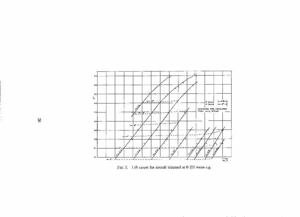
4.2. Incidence and Lift-Curve Slope.

The results obtained from the measurement of incidence are shown in Fig. 3 plotted in carpet

form. Note that the CL's are trimmed values and that the incidence is measured from the wing datum.

The Reynolds number varies throughout the carpet of Fig. 3 decreasing from a mean value of

about 30 x 106 at C L = 0.1 to about 13 x 106 at C L = 0.5. The specific values of R corresponding

to the various C•'s and Mach numbers can be obtained from Fig. 5. Estimates using Ref. 11 suggest

that the effects of this Reynolds number variation are negligible. Estimates also show that the c.g.

variation as fuel is consumed is insufficiently large to warrant any corrections to C L to reduce these

values to a constant c.g. position.

Fig. 3 shows that the incidence for zero lift is about 0.4 ° at all Mach numbers. This compares quite well with the values obtained from wind-tunnel tests 9,1°, 12. The lift-curve slopes derived

from Fig. 3 are shown plotted in Fig. 4a. It is seen that (aCL/O~),l, z increases with Mach number up to M = 0.9 and then decreases slightly. In this respect it should be noted that at M -- 0.94 the

C L range over which incidence measurements were made was small by comparison with experi- mental scatter. Thus, as the lift-curve slope obtained at this Mach number may not be very reliable, the fall in (OCL/OO~)_~/£ at the higher Mach number cannot be regarded as being conclusively proved.

Also shown in Fig. 4a are the results of wind-tunnel tests on two Hunter models 9, lo. To facilitate

comparison with these, the flight results have been corrected to the tail-off condition, using the data of Ref. 9. The wind-tunnel results of Ref. 9 are seen to give a 5 to 10% lower lift-curve slope than the flight tests. Estimates based on Ref. 11 suggest that the geometrical differences between the wind-tunnel model and the full-scale aircraft would be sufficient to account for a 3% difference

in 3CLIO % the remaining difference being possibly due to scale effect 1~. The tests of Ref. 10 were on a more representative model at a higher Reynolds number, and are seen to give a value of

3CL/3~ in fairly good agreement with that obtained by extrapolation of the flight results. The

tunnel results quoted above were all with transition free.

Fig. 4b shows the flight results (corrected to tail-off condition) compared with estimates for the

wing alone as derived from Refs. 11 and 13. In making these estimates transition on the wing was

assumed to be at the leading edge (see Section 4.1). Comparison shows that the estimated lift-curve

slopes are consistently lower than the flight results. Inclusion of the fuselage is would only increase

7

the estimated lift-curve slope by about 4%, leaving a large discrepancy between estimates and flight tests still unaccounted for.

As it was not found possible to measure incidence directly in flight at transonic and supersonic

speeds, some assumptions were necessary in this respect in order that drag measurements could be

made using the accelerometer technique. In the absence of any directly applicable experimental

data on lift-curve slope, the existing experimental curve (tail on) was faired smoothly into the

supersonic curve estimated from Ref. 13. A further assumption made was that the zero-lift angle

remained constant at 0.4 ° at all Math numbers. Clearly, these extrapolations and assumptions are

not completely satisfactory but they present the best that can be done under the circumstances.

The errors in drag introduced by errors in these assumed values of incidence are discussed in the Appendix.

4.3. Drag.

4.3.1. Drag due to l i f t . - -The drag results obtained from stabilised levels are presented in Fig. 5. It will be seen that at low C L the compressibility drag rise commences soon after M = 0.8. As C L increases, the drag rise commences progressively earlier until at C L = 0.5 the drag starts to increase soon after M = 0.45.

The results of Fig. 5 are shown in Fig. 6a plotted as C a versus CL ~ for constant Math numbers. The values plotted are those obtained from the faired lines drawn in Fig. 5, the low Mach number

values being those below the drag rise. Straight lines have been drawn through the various sets of values on the assumption that drag obeys the law

where

K CD~ = C~z + ~ C~ ~

CDT = total aircraft drag coefficient

CDz = drag coefficient at zero lift

K = effective induced-drag factor.

The values of K obtained from the slopes of the lines are 1- 15 at low M, 1.37 at M = 0.85 and 1.52 at M = 0"90.

The experimental scatter present in Fig. 5 amounts to about + 4% in CD. This scatter makes

the value of K obtained very critical both to the weight that we give each experimental point in drawing the mean lines of Fig. 5 and also to the range of C L covered. The value of K obtained at

low Math number is the mean over a larger C n range than at M = 0.85 or 0.90 and might therefore be expected to be more accurate.

The flight technique whereby drag is measured at various Math numbers at a series of fixed values of C D results inevitably in a variation of Reynolds number. It so happens that the change in Reynolds number with Mach number at constant C n is relatively small (Fig. 5), but with increasing CL at constant M the reduction in Reynolds number is quite large (Fig. 6a). The values of K obtained from Fig. 6a thus include any effects on total drag arising from these Reynolds number variations. An attempt has been made to reduce the results to a constant Reynolds number of 34 x 106 by using R.Ae.S. Data Sheets and assuming that only the drag at zero lift is affected by Reynolds number 15. In making this correction, transition was assumed to be at the leading edge of

8

the wings and tail and at the nose of the body, and the surfaces were assumed to be aerodynamically

smooth (Section 4.1). The values of CDT SO corrected are shown plotted in Fig. 6b. The values of K

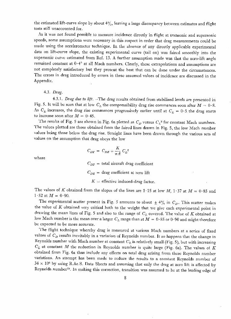
obtained are as follows:

M

Low M

0.85

0-90

Uncorrected for R (Fig. 6a)

1"15

1"37

1"52

K

Corrected to R = 34 × 106 (Fig. 6b)

1.09

1.19

1.23

The variation of the drag of the complete aircraft with Reynolds number will in practice be

rather less than that for an aerodynamically clean aircraft due to the effects of control-surface gaps,

skin joints and other surface irregularities (Section 4.1). The true values of K at constant Reynolds

number will thus probably lie somewhere between the two extremes given above.

The value of 1.09 for K at low Mach number compares with 1-1 for the Supermarine 510,

1.25 for the DH.108, and 1.33 for the Hawker P.1052, all values being corrected to constant R

(Ref. 15). The reason for this large variation of K from aircraft to aircraft is not readily apparent.

Fig. 7 presents a plot of C~ versus CL 2 showing the results of Fig. 5 extended to higher CL'S by

additional stabilised levels and by partial glides. Note that no correction for Reynolds number has

been applied, because of the uncertainty in applying this at high CL'S. The CD/CL 2 curve is seen

to be linear up to a certain CL, above which the drag increases rapidly and departs more and more

from the linear value. This drag increase results from the occurrence and subsequent spread of

separated flow on various parts of the aircraft. The drag rise commences earlier as Mach number

increases, confirming the well known result that separation also occurs at an earlier C L. The values

of C L for the onset of buff~et (as obtained from unpublished R.A.E. tests) are also shown plotted in

Fig. 7. It is seen that the drag rise does not become apparent to the pilot as buffet until the drag

has risen by a finite amount. A larger drag rise is necessary at low M than at high M, probably

because of the lower E.A.S. and hence lower intensity of buffet.

At transonic and supersonic speeds a small range of C L from about 0.05 to about 0.20 was covered in dives and pull-outs. This has enabled some approximate values of K to be obtained at supersonic speeds, and the results are given in Fig. 8. It is seen that the results are in fairly good agreement with the empirical data of Ref. 16. The measured values of K beyond M = 1.0 are of the same magnitude as those that would be expected for the wing alone with no leading-edge suction, {K = 7rA/(OCz/OeOwing }. This suggests that if the drag due to lift on the fuselage and tail were negligible the high values of K on the Hunter could be explained by the loss of virtually all the leading-edge suction on the wing beyond M = 1.0, although this result would be rather surprising.

It should be emphasised that the actual values of K derived from these dives and pull-outs are dependent largely upon the values of % and OCz,/ao~ that are assumed, errors in these two quantities

9

having an appreciable effect on K (Appendix). However, it is of interest to note that any errors in

aCL/aC~ alone would not be expected to influence the general result, noted above, that K ~-- aCL/a%

although the picture could be altered by errors in the assumed values of %.

4.3.2. Drag at CL'S o f 0 and O" 1 . - -The established level results at C L = 0.1 (Fig. 5) are

shown in Fig. 9 extended to transonic and supersonic speeds by dives using the accelerometer

technique. As steady dives at C L = 0.1 were not found possible beyond M = 1.05, the drag from

M = 1.05 to 1.23 was obtained from dives and pull-outs, the results being reduced to C L -- 0.1

by assuming the values of K given in Fig. 8.

Fig. 9 shows that the drag obtained from stabilised levels agrees closely with that obtained from

the dives. The drag coefficient at C L = 0.1 is seen to commence to rise soon after M = 0" 8, the

drag increasing rapidly between M = 0.92 and 0"99 and attaining a peak value of 0"0565 at

M = 1.15. Further increase of Mach number up to M = 1.23 causes a slight reduction in C v .

Also shown in Fig. 9 is the zero-lift drag coefficient obtained by using the values of K given in

Fig. 8 to extrapolate the results from C 5 = 0.1. The low Mach number value of U p s is seen to

be about 0.0125 (at R = 34 x 106). This rises to a peak value of 0.0545 at M = 1.15.

4.3.3. Accelerated and decelerated l e v e l s . - - T h e results obtained from an accelerated and a

decelerated level at both 15 000 ft and 40 000 ft are given in Fig. 10. Also plotted, where appro- priate, are the values derived from the results of stabilised levels (Fig. 5). The extent of the agreement

with stabilised levels is illustrated more clearly in Fig. 11, where the results have been reduced to

Cz~ z by assuming the values of K given in Fig. 6a. It is seen that, although the general agreement with stabilised levels is reasonable, the scatter is

large. This large scatter arises mainly from the difficulty of fairing the readings of A.S.I. and altitude and of drawing tangents to these fairings. This difficulty is accentuated by the hysteresis lag of the

standard altimeter making it impossible to detect rates of change of altitude within this hysteresis band. The skill of the pilot in maintaining altitude strictly constant plays a large part in obtaining

good results from this method. It is of interest to note that the four runs shown in Fig. 10 were accomplished in one flight. In

the same amount of flying time only about four stabilised level points could have been produced.

The argument for using accelerated levels therefore lies in the large amount of data (of admittedly

limited accuracy) that can be produced in a small number of flying hours. Thus one flight or so

consisting of a good accelerated level at, say 10 000, 20 000, 30 000 and 40 000 ft would enable us

to deduce

(a) the variation of C~9 z up to the maximum level-flight Mach number

(b) the level-flight thrust boundaries of the aircraft for the engine settings and altitudes chosen.

In deriving this data a value for K would need to be assumed or estimated. A further assumption

with regard to (b) would be that the intake efficiency did not vary appreciably with C L . The accuracy with which the data could be obtained and the number of flights necessary would depend largely

upon the skill of the pilot. Decelerated levels are not in general of great value as the intakes are working under unrepresenta-

tive conditions, possibly leading in some cases to an appreciable increase in spillage drag. Further inspection of Figs. 10 and 11 suggests that the decelerated levels give in general a slightly higher drag for the Hunter than do the accelerated levels. This difference however may be due largely to

experimental inaccuracies.

10

4.3.4. Comparison of flight and wind-tunnel results.--Fig. 12 compares the high Mach

number drag rise obtained from flight tests with ~that obtained from high-speed wind-tunnel tests 9.

T h e model used in the wind- tunnel tests was without tail and, as the tests were made several years

ago, was not completely representative of the full-scale aircraft. The main differences were that

on the model the tip sections were 10% thick and the sweep 42.5 °. Th e drag rise is seen to compare

well at low CL'S but to commence progressively earlier in flight than in the tunnel as C L is increased.

This is contrary to other comparisons 17 between wind-tunnel data at low Reynolds number and

flight data. It is felt that the relatively good agreement at low lift shown in Fig. 12 may be largely

fortuitous in view of the large and unpredictable scale effects e° to be expected on transition-free

model tests at Reynolds numbers as low as 0.5 x 106.

T h e values of effective induced-drag factor, K, obtained from various low Mach number wind-

tunnel tests are shown in Fig. 13 plotted against Reynolds number. Except where otherwise stated,

the tests are all with transition free. All the results shown are for configurations similar to, if not

identical to, that of the Hunter. Also shown in Fig. 13 is the value of K obtained from the present

flight tests. It is seen that apart f rom the isolated point at R = 0.5 x 106, the tunnel results agree

well amongst themselves, the mean value of K decreasing from 1.30 to about 1.08 as Reynolds

number is increased from 1.4 x 106 to 10 x 106. At the highest Reynolds number attained in the

tunnel tests the value of K is of the same order as that obtained from the flight tests.

T he high values of K at low Reynolds numbers are probably the result of changes in profile drag

due to forward movement of transition as C L is increased. Th e considerably reduced value when

transition is fixed at a forward position tends to confirm this.

4.4. Level-Flight Performance.

Fig. 14 shows the level-flight performance of the Hunter Mk. I plotted in non-dimensional form.

T he experimental points shown are derived from fur ther analysis of the flight data which was

obtained for determination of the stabilised level results shown in Fig. 5. The performance carpet

has been plotted with C L as one of the variables instead of the more usual W/P, but it is a simple

matter to convert one into the other as W/P o~ CLM 2.

5. Conclusions.

Flight tests made to measure the drag of a Hawker Hunter F Mk. I aircraft give the following

results:

(i) Cgz at low Mach number at R = 34 x 106 is 0-0125.

(ii) At C L = 0- 1, a gradual drag rise commences soon after M -- 0- 8, the drag increasing rapidly

beyond M = 0 .92 and attaining a peak value of C 9 of 0.0565 at M = 1.15. Fur ther increase of

Mach number up to 1.23 causes a slight reduction in drag. Comparison of the compressibility drag

rise obtained f rom wind-tunnel tests and from flight shows good agreement, although this may be

largely fortuitous in view of the low tunnel Reynolds number.

(iii) -The Cg/CL 2 curve becomes non-linear at the higher CL'S , the C L for divergence decreasing

with increase in Mach number. At M = 0- 3 the divergence C L is 0 .76 falling to 0.41 at M = 0.70.

Over the low C L range at low Mach number the effective induced-drag factor K corrected to constant

Reynolds number is 1.09.

(iv) Some approximate values of K at supersonic speeds suggest that virtually all the leading-edge

suction on the wing is lost beyond M = 1-0.

11

(v) The accelerated and decelerated levels technique gives values of CDz similar to those obtained from stabilised levels although the scatter is large.

(vi) The lift-curve slope of the complete aircraft increases from 3.5 at M = 0.3 to 4.6 at M = 0-9. The zero-lift angle is about 0.4 °. Wind-tunnel and flight measurements of lift-curve slope are in reasonable agreement when allowance is made for differences in geometry and in Reynolds number.

12

Pc~

Po

P

To

0

M

W

S

A

~st4

t/c

K

(Z

Ot o

N

R

dh

d t

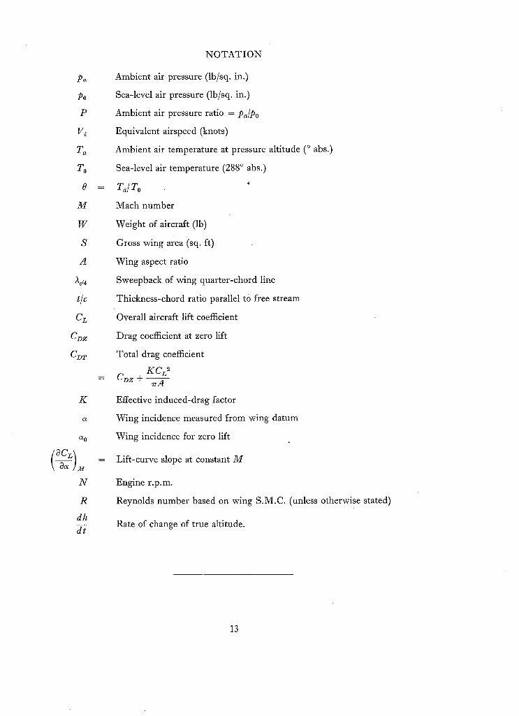
NOTATION

Ambient air pressure (lb/sq. in.)

Sea-level air pressure (lb/sq. in.)

Ambient air pressure ratio = Pa/Po

Equivalent airspeed (knots)

Ambient air temperature at pressure altitude (° abs.)

Sea-level air temperature (288 ° abs.)

= T~,/T o

Mach number

Weight of aircraft (lb)

Gross wing area (sq. ft)

Wing aspect ratio

Sweepback of wing quarter-chord line

Thickness-chord ratio parallel tO free stream

Overall aircraft lift coefficient

Drag coefficient at zero lift

Total drag coefficient

K CL ~ = C z+ ---y-

Effective induced-drag factor

Wing incidence measured from wing datum

Wing incidence for zero lift

= Lift-curve slope at constant M

Engine r.p.m.

Reynolds number based on wing S.M.C. (unless otherwise stated)

Rate of change of true altitude.

13

No. Author(s)

1 D. J. Higton, R. H. Plascott and D. A. Clarke

2 G. W. Trevelyan and D. R. Blundell

3 D . J . Higton and R. J. Ross

4 D. R. Andrews and J. E. Nethaway

5 A. D. Young, G. L. Green and Miss E. Young

6 W.E. Gray . . . . . .

7 P.R. Owen and D. G. Randall

8 P.R. Owen and D. G. Randall

9 J .R. Collingbourne . . . .

10 D.A. Kirby and J. F. Holford

11 J .R . Collingbourne . . . .

12 C. Salter, C. J. W. Miles and Miss H. M. Lee

13 A. Stanbrook . . . . . .

R E F E R E N C E S

Title, etc.

The measurement of the overall drag of an aircraft at high Mach numbers.

A.R.C.R. & M. 2748. January, 1949.

Determination of the drag of jet propelled aircraft in flight. Aero. (Quart., Vol. 1, Part 1. May, 1949.

The measurement of drag in flight on a swept wing aircraft (Hawker P1052) at high Mach numbers.

R.A.E. Report Aero. 2351.

A.R.C. 13 059. January, 1950.

Flight measurements of the pressure errors of a nose and a wing boom airspeed system on a swept-wing aircraft (Hunter F Mk. I) at Mach numbers up to 1-2.

R.A.E. Tech. Note Aero. 2354.

A.R.C. 17 629. January, 1955.

High speed wind tunnel tests of the effect of camouflage paint roughness on drag.

R.A.E. Report Aero. 1977. A.R.C. 8 152. October, 1944.

The effect of wing sweep on laminar flow. A.R.C. 14 929. February, 1952.

Boundary layer transition on a sweptback wing. A.R.C. 15 022. May, 1952. ,

Boundary layer transition on. a sweptback wing: effect of incidence. A.R.C. 16 191. October, 1953.

High speed wind tunnel tests up to M = 0.95 on a 1/15th scale model of the Hawker P.1067 (F3/48) (Preliminary design).

R.A.E. Report Aero. 2342. A.R.C. 12 947. November, 1949.

Low speed tunnel tests on a 1/5th scale model of a single-jet fighter with a 40 ° sweptback wing (Hawker F3/48).

R.A.E. Report Aero. 2382. A.R.C. 13 734. June, 1950.

The estimation of lift curve slope at subsonic Mach numbers. R.A.E. Tech. Note Aero. 2145. A.R.C. 15 053. January, 1952.

Tests on a swept-back wing and body in the Compressed Air Tunnel. A.R.C.R. & M. 2738, May, 1950.

An analysis of theoretical and experimental data on the lift of wings with parallel tips at supersonic speeds.

R.A.E. Tech. Note Aero. 2105. A.R.C. 14 396. June, 1951.

14

No. Author(s)

14- K. Smith . . . .

15 R.J . Ross . . . . . .

16 M. M. Callan and R. J. Templin

17 R. Hills . . . . . .

18 J. Weber, D. A. Kirby and D. J. Kettle

19 R . C . A . Dando . . . .

20 A. B. Haines, D. W. Holder and H. H. Pearcey

R E F E R E N C E S - - c o n t i n u e d

Title, etc.

Pressure lag in pipes with special reference to aircraft speed and height measurements.

R.A.E. Report Aero. 2507. A.R.C. 17 610. November, 1954.

A note on the effect of sweepback on the induced drag factor. R.A.E. Tech. Note Aero. 2070. A.R.C. 13 739. September, 1950.

A collection and analysis of experimental data on the aerodynamic characteristics of finite wings. Part l -- l i f t curve slope and drag due to lift of swept wings at supersonic speeds.

N.A.E. (Canada) Lab. Report LR.93. January, 1954

A note on flight-tunnel comparison and scale effect on swept wing designs.

R.A.E. Tech. Note Aero. 2077.

A.R.C. 13 479. October, 1950.

An extension of Multhopp's method of calculating the spanwise loading of wing-fuselage combinations.

A.R.C.R. & M. 2872. November, 1951.

Two methods of boundary layer transition indication suitable for routine tests in flight.

R.A.E. Report Aero. 2321. A.R.C. 12 531. April, 1949.

Scale effects at high subsonic and transonic speeds and methods for fixing boundary-layer transition in model experiments.

A.R.C.R. & M. 3012. September, 1954.

15

where

A P P E N D I X

Effects of Errors in Dwidence on the Accuracy of Drag Measurements using the Accelerometer Technique

It can be shown from the equations of Ref. 1 that, to a first approximation

W--

R =

¢=

FN + WR qS

Nett thrust

Weight of aircraft

Longitudinal accelerometer reading

Incidence of fuselage datum to flight path (radians).

Thus an error A¢ in incidence gives rise to an error of C L A¢ in C D. Th e accuracy of drag

measurements using the accelerometer technique is thus closely related to the accuracy of the values

of incidence that are assumed.

In this report, the drag at transonic and supersonic speeds has been derived using estimated

values of incidence. The following table gives some idea of the effects of errors in the estimated

values used for lift-curve slope and no lift angle at supersonic speeds.

Error in estimated value

of incidence

_+ ½° in s0

+ 5 0 ~ in OC5/Os

- 5 0 ~ in 8CL/ao~

Resulting error in

CDat CL = 0.1

+ 0.0009

- 0. 0022

+ 0. 0007

K

+0 '5

- 2 " 3

+0-8

It can be seen that quite large errors in incidence can be tolerated without seriously impairing the

accuracy of C D at C L = 0- 1. This is particularly true when CDz is obtained from measurements of

C D at two or more C5's, as these errors in ~CL/OS can be shown to cancel.

The above table also shows that K is very critical to errors in % and OCL/Os. It would appear

that accurate values of K can only be obtained with the accelerometer technique if incidence is

measured directly in flight or can be estimated from reliable experimental data.

16

T A B L E 1

Details of Hunter WT.571

Aircraft Wing area

Wing span

Aspect ratio

Taper ratio

Sweepback at quarter-chord

Standard mean chord

Wing setting to fuselage datum

Max. thickness/chord ratio (symmetrical)

Position of max. t/c

A.U.W. (Take-off)

Fuel contents

C.G. position at take-off

C.G. position with rear tanks empty (274 gal left)

C.G. position with rear and centre tanks empty (202 gal left)

C.G. position no fuel

Engine

Rolls Royce Avon 107 RA7

Nominal static thrust at sea level

The operational limitations of the engine are as follows :

Take-off and operational necessity

Max. intermediate

Max. continuous

r.~.m.

7950

7750

7500

Max.

J.P.T. 680°C

620°C

575°C

340 sq. ft

33 f t8 in.

3"33

0-41

40 °

10-1 ft

1½ °

8.5% 37" 5 ~ chord

15 520 lb

334 gal

0" 298

0" 270

0- 267

0-314

7500 lb

Time Limit 10 min

30 min

Unrestricted

17

(92174) B

FIG. 1. General arrangement of Hawker Hunter F. Mk. I (WT.571).

18

-.

c .

FIO. 2. General view of Hunter WT.571.

1 " O

o ~

c~7

o . i

o ~ . : 0 ° --

,,/" / ,.

_ ~ : ' , o : _ . / . - - 7

s ~ / / - , . . . . . . . . . / / / / / ,~,

" < - : ' - - , - - _7'--- 7, .7 / : / / / / ~ , ~2 / / I ¢~i17

FIG. 3. Lift carpet for aircraft trimmed at 0.27~ mean c.g.

@0

&O

6"0

TIML OFF"

4 . 0

?.-0

0 -" 0-15 O'R

FLlr~H'I" ~[~JL"~ FROH

Fie. 4a.

I I

0 -~. 0 '6 0 "8 h l I .o ~'~

(OC~/O~)~ vs. M--comparison of flight and tunnel results.

0 O-P_

FL~ f~JLT~

I o.4- 0 - 6

/ E,.~TIr"I~,,'i'E ~- I=OR WLN~

o.8 1.0 f"3 I'R Fie. 4b. (SOL/8O@± vs. M--comparison of

flight tests with estimates (tail off).

O-OS

15.5 0 . 0 4 []

0.0%

O.O~

CL.: C,.~,

O.Ol

° 0 .]

J

/

,%

CL + ~'1 0 0'15 x O'& A 0~,

0 0 . 5

_q..o4s_

II

,"1 Zl Z05'14" ~~t? S I~A .L&'5 2.1.!1 21

~o ~ a ~ " o o ~ ~ 1

b l / "

R~-YNoL.r~5 N U M B ~ ~UO'T~E~ NF_~i~. - - ~P~R~MF.NT~.%, POINT~ ( . x I0 -¢') -

0.4- O-S o -6 o ' 9 o , 8 M o..9 0'95

FIC. 5. Drag obtained from stabilised levels.

0"04-

0.05

C~. r

0.0~

O.01

/ s>T/ .,': +,,.v"

7 7 /

/

M~AN R~YNOLO~ N~('-~BER$ (~UO'I'EO NEaR ~OINT~ (~.11~6)

Fig. 6a. Drag coefficient vs. Cr2--results derived from FIC. 5.

0-O~

o.o=~ ~ .~/

COT / ~

0-0~- ~

|

0-01

R ~SU L~'S r-ORR ~Q'r ~.D "TO R. = ~4- ~. IO e .a.~G~i'-11NCa AEROOYN~MlCkLtY 5MOOTM .SLJ ~ ;=At- E ~P AN~ TRF~NSITION

Q. i o-a 0..~ o-:~

Fig. 6b. Drag coefficient v s . Cz2--results of FIG. 6a corrected to R = 34 x 106.

0-.~0

0.~.0

Ct~ T

O'lO

/

o ~ ~

ONSET OF B~ 'F~T

\

/~.i Z Q m = o.s

Q M=o.5 ~0, ~ ~ X VAI.ur~ F'ROt-%

" (UNCORReCTeD FOR R~YN~3LO5 j NLI M ~ F-.F~ V~RI~TION)

I I O 0.I 0"~- 0-~ o.~- 0.5 O.C~ q7 ~ O'B u-~

FIG. 7. Drag coefficient vs. CL 2 at high CL's.

5.o

'4"0

K

3.0

P.'O

X $'Th.BILISED LEVEL5 CGRREC.T~ "TO

JKNII~ PULL- OLI'TS

I-0 0'7

J o.~ o.~

~CL '

\1 ~m Pl RIC~,L ~NT~,

OF iEE 16

FO r~ N I'~ Fa

FIG. 8. Variation of effective induced-drag factor with Mach number.

23

b ~ . .N

o . Q

0 -05

CD, r

0 .Q,R.

O .05

0 -0~

0 .QI

0 0 . 2

! jS

C~_: 0.5

0.4-

i

l 0.5 O'G o '9 O'B o,.,~ i.Q M

/~

i r

/!

X C)IW~- ~ ° c-T~B]LI~E~ LEV~L~ (F,q]~)

I ' | I ' ~

FIG. 9. Drag obtained from dives using accelerometer technique.

t 'O G~

0"0~

0 ' 0 3

CD T a ~

i

0~01 -o.z

o 0 . 5 5 0 " 4

0-05

O-Oq-

c%

0"05

O-OP_ o4--

C~

o.0~ 0-a-

o 0 "-~5 0 . 4

FIG. 10.

-<Z2"

o. 5 o "G o .'J

~&,TIT~J~ I~ 0 0 0 FT

+ 5T~tMLIS~ ~-=..vE&..

?

o-B H o.9 0

0.5

K \

o ~

~,LTITUDE 4 - 0 0 0 0 FT

O ~,C.£F.LERJ~TED L.~F-~_ K DEC.ELER~,TED ~.F.W~-~.

0.~ O. 0,8 N 0.9 Off5

Results obtained from accelerated and decelerated levels.

0-04-

0-05

C b z

0.0~.

o A~-~.EL.ERATEZ) L~'VEL. I S O ~ I & A ~ E L ~ ' R ~ T ~ LEVEL 4 0 ~ I X ~EC~LI~RAT~D L~VEL 1 5 0 Q O ' "P ~F.CF.LER~,'rE~ LEVF~ 4 0 0 0 0 '

. . . . . . ~_o_ o _~__o __ a__*_~_, O-oI 0 ~ , 0 w . o- O o O ~

O. o .:~ 0. ,4-

i

+

A

a-

P + / / ~

o o o ® o

0 - 5 o -6 0 - 7 0 . 8 o-.9

FIG. 11.

M 1.0

CDz derived from accelerated and decelerated levels compared with that from stabilised levels.

0 ' 0 4 .

0.0=~

0-0~-

O-OI

. . . . W lN~- " f~Nt~Et= RESU~=TS (~O0EI= "WrrHO~T T/=4~.) REF. ~ . N. = O '~1 ~ IO 6

/ / /

/ /

/

/ / ]

I / / / /I

/

/I / / / /

O -- / [ /

/ / .

CL. = 0 ' ~ / /

/ / /

/ CL..= 0-1

0 0 -4 - 0 - 5 0 . 6 0 -7 O - 8 0 . 9 H r o

C~ = 0 . 4 -

FIG. 12. Comparison of drag rise with Mach number from flight and wind-tunnel tests.

P-,O

x

E FFEI3"Tt'VE

O P, AG, FA~QR

K I.G

1"4

I'e.

1.0 0 . 5

FIG. 13.

80DY

x TI',r.PLAN E

..... 4 1

. ~ 0"4.1 =.-~- 85 8'5 qO tO

~ , ~ F U I 4 . ~ k 41 :~

~ .~ V~,~.~E

TR AN~I'TIOH ~'I~ED AT 15~oc.I t

Comparison of flight and wind-tunnel induced-drag data at low M.

bl

ul

bO " 4

~000

8OOC

7000 / /=

6430O

( /~°° I

FIG. 14. Hunter F. Mk. I.--level-flight performance carpet•

Publications of the Aeronautical Research Council

A N N U A L T E C H N I C A L R E P O R T S O F T H E A E R O N A U T I C A L R E S E A R C H C O U N C I L ( B O U N D V O L U M E S )

1945 Vol. "I. Aero and Hydrodynamics, Aerofoils. £6 ios. (£6 x3s. 6d.) Vol. II. Aircraft, Airscrews, Controls. £6 Ios. (£6 I3s. 6d.) Vol. I lL Flutter and Vibration, Instruments, Miscellaneous, Parachutes, Plates and Panels, Propulsion.

£6 ios. (£6 I3s. 6d.) Vol. IV. Stability, Structures, Wind Tunnels, Wind Tunnel Technique. £6 IOS. (£6 13s. 3d.)

z946 Vol. i. Accidents, Aerodynamics, Aerofoils and Hydrofoils. £8 8s. (£8 IIs. 9d.) Vol. II. Airscrews, Cabin Cooling, Chemical Hazards, Controls, Flames, Flutter, Helicopters, Instruments and

Instrumentation, Interference, Jets, Miscellaneous, Parachutes. £8 8s. (£8 zxs. 3d.) Vol. III. Performance, Propulsion, Seaplanes, Stability, Structures, Wind Tunnels. £8 8s. (£8 ixs. 6d.)

1947 Vol. I. Aerodynamics, Aerofoils, Aircraft. £8 8s. (£8 Izs. 9d.) Vol. II. Airscrews and Rotors, Controls, Flutter, Materials, Miscellaneous, Parachutes, Propulsion, Seaplanes,

Stability, Structures, Take-off and Landing. £8 8s. (£8 1is. 9d.)

t948 Vol. I. Aerodynamics, Aerofoils, Aircraft, Airscrews, Controls, Flutter and Vibration, Helicopters, Instrumer=ts, Propulsion, Seaplane, Stability, Structures, Wind Tunnels. £6 zos. (£6 I3s. 3d.)

Vol. II. Aerodynamics, Aerofoils, Aircraft, Airscrews, Controls, Flutter and Vibration, Helicopters, Instruments, Propulsion, Seaplane, Stability, Structures, Wind Tunnels. £5 ios. (£5 13s. 3d.)

I949 Vol. I. Aerodynamics, Aerofoils. £5 zos. (£5 I3S. 3d.) Vol. II. Aircraft, Controls, Flutter and Vibration, Helicopters, Instruments, Materials, Seaplanes, Structures,

Wind Tunnels. £5 ios. (£5 13s.)

195o Vol. I. Aerodynamics, Aerofoils, Aircraft. £5 Izs. 6d. (£5 I6s.) Vol. II. Apparatus, Flutter and Vibration, Meteorology, Panels, Performance, Rotorcraft, Seaplanes.

£4 (£4 3s.) Vol. III. Stability and Control, Structures, Thermodynamics, Visual Aids, Wind 'runnels. £4 (£4 2s. 9d.)

I951 Vol. I. Aerodynamics, Aerofoils. £6 ios. (£6 I3s. 3d.) Vol, II. Compressors and Turbines, Flutter, Instruments, Mathematics, Ropes, Rotorcraft, Stability and

Control, Structures, Wind Tunnels. £5 IOS. (£5 I3s. 3d.)

x951 Vol. I. Aerodynamics, Aerofoils. £8 8s. (£8 ixs. 3d.) Vol. II. Aircraft, Bodies, Compressors, Controls, Equipment, Flutter and Oscillation, Rotorcraft, Seaplanes,

Structures. £5 ios. (£5 I3S.)

I953 Vol. I. Aerodynamics, Aerofoils and Wings, Aircraft, Compressors and Turbines, Controls. £6 (£6 3s. 3d.) Vol. II. Flutter and Oscillation, Gusts, Helicopters, Performance, Seaplanes, Stability, Structures, Thermo-

dynamics, Turbulence. £5 5s. (£5 8s. 3d.)

I954 Aero and Hydrodynamics, Aerofoils, Arrester gear, Compressors and Turbines, Flutter, Materials, Performance, Rotorcraft, Stability and Control, Structures. £7 7s. (£7 lOS. 6d.)

Special Volumes Vol. I. Aero and Hydrodynamics, Aerofoils, Controls, Flutter, Kites, Parachutes, Performance, Propulsion,

Stability. £6 6s. (£6 9s.) Vol. II. Aero and Hsidrodynamics, Aerofoils, Airscrews, Controls, Flutter, Materials, Miscellaneous, Parachutes,

Propulsion, Stability, Structures. £7 7s. (£7 lOS.) Vol. III. Aero and Hydrodynamics, Aerofoils, Airscrews, Controls, Flutter, Kites, Miscellaneous, Parachutes,

Propulsion, Seaplanes, Stability, Structures, Test Equipment. £9 9s. (£9 1as. 9d.)

Reviews of the Aeronautical Research Council I949-54 5s. (5s. 5d.)

Index to all Reports and Memoranda published in the Annual Technical Reports I9O9-1947 R. & M. a6oo (out of print)

Indexes to the Reports and Memoranda of the Aeronautical Research Council Between Nos. a45I-a549: R. & M. No. a55o as. 6d. (as. 9d.); Between Nos. a65i-a749: R. & M. No. a75o as. 6d. (as. 9d.); Between Nos. 2751-2849: R. & M. No. 285o zs. 6d. (as. 9d.); Between Nos. 2851-2949: R. & M. No. a95o 3s. (3s. 3d.); Between Nos. 2951-3o49: R. & M. No. 3o5 o 3s. 6d. (3s. 9d.); Between Nos. 3o51-3149: R. & M. No. 315o 3s. 6d. (3s. 9d.); Between Nos. 3151-3249: R. & M. No. 325o 3s. 6d. (3 s. 9d.); Between Nos. 3a51-3349: R. & M.

No. 335o 3s. 6d. (3s. iod.)

Prices in brackets include postage

Government publications can be purchased over the counter or by post from the Government Bookshops in London, Edinburgh, Cardiff, Belfast, Manchester, Birmingham and Bristol, or through any bookseller

R. & M. No. 3420

© Crown Copyright x966

Printed and published by HER MAJESTY'S STATIONERY OFFICE

To be purchased from 49 High Holborn, London wc i 423 Oxford Street, London wx I3A Castle Street, Edinburgh z

io 9 St. Mary Street, Cardiff Brazennose Street, Manchester 2

5o Fairfax Street, Bristol i 35 Smallbrook, Ringway, Birmingham 5

80 Chiehester Street, Belfast I or through any bookseller

Printed in England

Ro & Mo No, 3420

S.O. Code No. 23-34zo