flight-determined subsonic lift and drag … american institute of aeronautics and astronautics...

1

American Institute of Aeronautics and Astronautics

FLIGHT-DETERMINED SUBSONIC LIFT AND DRAG CHARACTERISTICS OF SEVEN LIFTING-BODY AND WING-BODY

REENTRY VEHICLE CONFIGURATIONS WITH TRUNCATED BASES

Edwin J. Saltzman

*

Analytical Services & MaterialsEdwards, California

K. Charles Wang

†

The Aerospace CorporationEl Segundo, California

Kenneth W. Iliff

‡

NASA Dryden Flight Research CenterEdwards, California

*

Abstract

†

This

‡

paper examines flight-measured subsonic liftand drag characteristics of seven lifting-body and wing-body reentry vehicle configurations with truncatedbases. The seven vehicles are the full-scale M2-F1,M2-F2, HL-10, X-24A, X-24B, and X-15 vehicles andthe Space Shuttle prototype. Lift and drag data of thevarious vehicles are assembled under aerodynamicperformance parameters and presented in severalanalytical and graphical formats. These formats unifythe data and allow a greater understanding than studyingthe vehicles individually allows. Lift-curve slope dataare studied with respect to aspect ratio and related togeneric wind-tunnel model data and to theory for low-aspect-ratio planforms. The proper definition ofreference area was critical for understanding andcomparing the lift data. The drag components studiedinclude minimum drag coefficient, lift-related drag,maximum lift-to-drag ratio, and, where available, basepressure coefficients. The effects of fineness ratio onforebody drag were also considered. The influence offorebody drag on afterbody (base) drag at low lift is

*

Edwin J. Saltzman, Senior Research Engineer.

†

K. Charles Wang, Member of the Technical Staff, Member,AIAA.

‡

Kenneth W. Iliff, Chief Scientist, Fellow, AIAA.

Copyright

1999 by the American Institute of Aeronautics andAstronautics, Inc. No copyright is asserted in the United States underTitle 17, U.S. Code. The U.S. Government has a royalty-free license toexercise all rights under the copyright claimed herein forGovernmental purposes. All other rights are reserved by the copyrightowner.

shown to be related to Hoerner’s compilation for body,airfoil, nacelle, and canopy drag. These analyses areintended to provide a useful analytical framework withwhich to compare and evaluate new vehicleconfigurations of the same generic family.

Nomenclature

aspect ratio,

base area, ft

2

maximum projected cross-sectional area, ft

2

longitudinal acceleration,

g

normal acceleration,

g

wetted area, ft

2

span, ft

base pressure profile factor,

drag coefficient,

base drag coefficient, using derived base pressure profile (reference area is for equations (8) and (9); reference area is for equations (11), (12), and (13))

base drag coefficient, assuming “flat” base pressure profile (reference area is )

zero-lift drag coefficient

forebody drag coefficient referenced to

A A b2

S⁄=

Ab

Ac

al

an

Aw

b

cc CDb

CDb′⁄=

CD CD D qS⁄=

CDbAb

S

CDb′

S

CD0

CD fore , bAb

2


forebody drag coefficient referenced to

minimum drag coefficient at vertex of drag polar

turbulent boundary-layer skin friction coefficient (over wetted surfaces)

equivalent skin friction coefficient (includes all drag components at

equivalent skin friction coefficient of the forebody alone

lift coefficient,

lift-curve slope (with respect to ), deg

–1

or rad

–1

lift coefficient for minimum drag coefficient

base pressure coefficient,

drag force along flightpath, lb

minimum drag at vertex of drag polar, lb

effective diameter,

equivalent parasite drag area, ft

2

gravitational acceleration

base pressure factor (numerator coefficient in Hoerner’s equation for three-dimensional configurations)

longitudinal length of a vehicle, ft

lift force normal to the flightpath, lb

lift-to-drag ratio

maximum lift-to-drag ratio

free-stream Mach number

ambient pressure, lb/ft

2

base static pressure, lb/ft

2

free-stream dynamic pressure, lb/ft

2

,

reference area, ft

2

vehicle weight, lb

angle of attack, deg

elevon or elevator deflection, deg

flap deflection, deg

lower flap deflection, deg

speed-brake deflection, deg

upper flap deflection, deg

uncertainty

increment in drag coefficient

drag-due-to-lift factor

Oswald lifting-efficiency factor, modified

wing or body sweep angle, deg

Introduction

In recent years, interest has been renewed incontrolled reentry from low-Earth orbit and the Earth’supper atmosphere. This interest has been motivated byseveral factors: a growing commercial space launchmarket and its desire for a low-cost, reusable means ofspace access; the need for a crew return/rescue vehiclefrom the International Space Station; and the potentialfor future military space operations. Fundamentalstudies by the NACA

§

and NASA in the late 1950’s andearly 1960’s described three basic methods ofatmospheric reentry: ballistic reentry, winged reentry,and wingless lifting-body reentry. The ballistic reentryapproach necessitates the use of parachutes to land, butthe lifting body and wing-body approaches provide thepossibility of horizontal landings. Flight examples ofthese latter two approaches include the M2-F1, M2-F2,HL-10, X-24A, X-24B, and X-15 vehicles and theSpace Shuttle.

¶

In addition, most lifting reentryconfigurations are attractive from the standpoint ofvolumetric efficiency, crossrange and downrangecapability, peak acceleration and heating rates, and low-speed handling qualities. Because of the current interestin lifting reentry shapes, this paper reexamines lift anddrag characteristics of the seven aforementionedvehicles during subsonic unpowered flight, and presentsa unified analysis of their subsonic aerodynamicperformance that enables meaningful comparisons withnew lifting reentry designs.

The vehicles examined in this paper, the M2-F1,M2-F2, HL-10, X-24A, X-24B, and X-15 vehicles andthe Shuttle prototype, comprise a unique class ofaircraft. Not only were the vehicles all lifting reentry

CD fore ,SS

CDmin

CF

CFeCDmin

CFe′

CL CL L qS⁄=

CLαα

CLmin

CPbCPb

pb p–( ) q⁄=

D

Dmin

deff deff 4Ac/π=

f

g

K

l

L

L D⁄

L D⁄( )max

M

p

pb

qq 0.7 pM

2=

S

W

α

δe

δ f

δL

§

The National Advisory Committee for Aeronautics (NACA)became incorporated into the National Aeronautics and SpaceAdministration (NASA) in October 1958.

¶

The Shuttle prototype referred to in this paper is the nonorbitingShuttle

Enterprise

. The Space Shuttle referred to is the Orbiter

Columbia

.

δsb

δU

∆

∆CD

∆CD ∆CL⁄ 2

ε

Λ

3


shapes, they were all piloted and capable of routineunpowered horizontal landings. Each of these vehiclesalso had a truncated afterbody or blunt base, whichresulted in base drag being a significant component ofthe total vehicle drag. In terms of planform design, all ofthe aforementioned vehicles had low-aspect ratiosbetween 0.6 and 2.5. The lift and drag data of thevehicles presented herein were obtained duringsubsonic, unpowered, coasting flights performed atEdwards Air Force Base (California) between 1959 and1977. The primary organizations involved were theNASA Dryden Flight Research Center

#

(Edwards,California) and the Air Force Flight Test Center; theU. S. Navy was also a partner in the X-15 program.

The purpose of this study is to assemble flight-measured lift and drag data from these vehicles undercommon aerodynamic performance parameters ormetrics (that is, the data from all seven vehicles areplotted together) in an attempt to unify the results forthis class of vehicles. This array of data is intended tocollectively yield information that might otherwiseescape notice if the vehicles were studied individually.To accomplish this, the performance parameters of thesubject vehicles have been related, or exposed, to dataformats and standards that are based on theory andconcepts that range from several decades to a centuryold (for example, the concepts of Jones; Allen andPerkins; Helmbold; Krienes; Oswald; and ultimately,Prandtl and Lanchester). Works that have been explicitlyused will be referenced in following sections.

The innovative and intuitive concepts cited abovewere intended for vehicle configurations that are quitedifferent than the subject vehicles. For example, therelevant Jones work applied to sharp-edged, low-aspect-ratio wings; Allen’s and Perkins’ related work addressedhigh-fineness-ratio bodies of revolution; and theconcepts of the others applied to moderate-, high-, andeven infinite-aspect-ratio wings. In other words, some ofthe concepts and standards employed herein were notoriginally intended to apply to the subject vehicles.Nevertheless, several such theoretical relationships andstandards have been used as a means of organizing andassessing the flight results considered.

This study is ultimately intended to provide a usefuldatabase and analytical framework with which tocompare and evaluate the subsonic aerodynamicperformance of new vehicle configurations of the same

generic family, low-aspect-ratio lifting reentry shapeswith truncated bases. The results can also be used as afirst-order design tool to help airframe designers definethe outer mold lines of future configurations as well asassess the predictive techniques used in design anddevelopment.

Use of trade names or names of manufacturers in thisdocument does not constitute an official endorsement ofsuch products or manufacturers, either expressed orimplied, by the National Aeronautics and SpaceAdministration.

Historical Background

At a NACA conference held in March of 1958,manned satellites and alternative methods of reenteringthe Earth’s atmosphere were comprehensively studied.

1

Three different methods of reentry from Earth orbitwere considered and discussed within the first fourpapers. The three methods were ballistic reentry,

2

thewingless lifting body,

3

and winged configurations.

4

Reference 3 advocated the lifting body mainly on thebasis that its hypersonic lift-to-drag ratio ofapproximately 0.5 would provide a maximumdeceleration of approximately 2

g

, low enough to allowa pilot to intervene in the control of the vehicle duringthis portion of the reentry.

The first lifting-body concepts involved very blunthalf-cones.

3, 5

Later, the concepts evolved into higher-fineness-ratio cones,

6–8

and the capability of achievingconventional (although unpowered) horizontal landingswas discussed. Numerous wind-tunnel model tests wereperformed on candidate versions of the half-cone andshapes having flattened bottom surfaces. In 1962, Reeddemonstrated unpowered horizontal landings andcontrollable flight with a miniature lightweight radio-controlled model of an M2 half-cone configuration.

9

This demonstration was followed by the construction ofa lightweight M2 craft large enough to carry a pilot.This unpowered M2-F1 vehicle demonstratedcontrollable flight and horizontal landings for amaximum subsonic lift-to-drag ratio of 2.8. The M2-F1lift, drag, and stability and control characteristics werepublished circa 1965.

10, 11

A heavier and modified version of the M2 shape wasbuilt and began flying in 1966. The resulting subsoniclift and drag data from flight were published in 1967.

12

Other lifting-body configurations (all capable ofunpowered horizontal landings) were developed andflight-tested as well. The subsonic lift and dragcharacteristics have previously been reported for the

#

NASA Dryden was called the NASA Flight Research Center at thetime of the subject flight experiments.

4


HL-10,

13

X-24A,

14

and X-24B

15

lifting bodies. Moreinformation on the evolution and flight testing of thelifting bodies is available.

9, 16–18

The M2-F1 and subsequent lifting bodies were not thepioneer vehicles for performing unpowered (“dead-stick”) landings, but they were the first very-low-aspect-ratio vehicles to routinely land withoutpower. The early rocket-powered research vehicles (theX-1, X-2, and D-558-II aircraft) were designed forunpowered landings, but they had aspect ratios between6 and 3.6. Later, the X-15 hypersonic research aircraft,which had an aspect ratio between the early rocket-powered vehicles and the lifting bodies, made routinedead-stick landings. The X-15 aircraft was designed toland unpowered

19

based on the experience of the earlierrocket-powered aircraft having the higher aspect ratiosand on a series of special landing investigations usinglow-aspect-ratio fighter-type airplanes.

20

This studyinvestigated approach and landings at lift-to-drag ratiosof 2 to 4 and used extended gear and speed brakes toincrease the drag. Lift and drag data for the X-15aircraft have previously been published.

19, 21

Despite the success of the X-15 unpowered landingexperience, the early planning for the Space Shuttleincluded “pop out” auxiliary engines to ensure safehorizontal landings. Thompson, an X-15 and lifting-body research pilot, argued that the X-15 and lifting-body experience rendered landing engines for the SpaceShuttle as an unnecessary weight and payload penalty.

22

The Space Shuttle was ultimately designed to makeunpowered landings, and thus became the heaviest ofthe reentry-type vehicles to use routine dead-sticklandings. The low-speed lift and drag characteristics ofthe nonorbiting Shuttle prototype

Enterprise

havepreviously been published.

23

Results have beenreported for the

Enterprise

with and without atailcone.

23

Only the truncated configuration—that is,without a tailcone—is considered in this paper.

Currently, new lifting reentry vehicles are beingdeveloped for rescue missions from space and to serveas reusable launch vehicles. These vehicles have muchin common with the lifting bodies described herein and,if aspect ratio is increased somewhat, with the X-15aircraft and the Shuttle prototype. This report presentsthe subsonic lift and drag characteristics of the M2-F1,M2-F2, HL-10, X-24A, X-24B, and X-15 vehicles andthe Shuttle prototype

Enterprise

under unifyingperformance parameters and formats, with the intent ofaiding the definition of exterior mold lines of future

candidate reentry vehicles that perform horizontallandings.

As was mentioned in the “Introduction,” some of theunifying metrics depend on borrowed concepts andstandards that are several decades old and wereoriginally intended for application on winged vehiclesof high- or moderate-aspect ratio. The authors realizeand accept that some readers may disagree with how theborrowed concepts and standards are applied herein.The formats, concepts, and standards that have beenused, and the information that may be derivedtherefrom, are offered as a beginning in the quest forunderstanding the general nature of lift and drag for thisunique class of vehicles. This “beginning” could nothave occurred but for the seven flight research programsaddressed herein and the dedicated technical personnelwho processed, analyzed, and carefully documented thelift and drag data. The present authors are indebted tothese earlier investigators for their attention to detail andcomprehensive reporting.

The following information is included for the purposeof orientation and perspective.

The seven vehicles completed a combined total of424 flights. Data from 6–7 percent of those flights wereused for this paper.

Methods of Analysis

This section assembles methods and metrics(performance parameters) used in the analysis of thesubject lift and drag data. The primary metrics ofaerodynamic performance include lift-curve slope; amodified Oswald lifting-efficiency factor; the drag-due-to-lift factor; maximum lift-to-drag ratio; and forminimum drag analysis, equivalent parasite drag area,equivalent skin friction coefficient, base pressure

A 1.5<( )

Earliest flight: June 8, 1959 X-15 aircraft

Last flight: October 26, 1977Shuttle prototype

Enterprise

Most numberof flights: 199 X-15 aircraft

Least numberof flights: 5

Shuttle prototype

Enterprise

Lightest vehicle: 1250 lbM2-F1

lifting body

Heaviest vehicle: 150,900 lbShuttle prototype

Enterprise

5


coefficient, base drag coefficient, and forebody dragcoefficient.

Lift-Curve Slope

Trimmed lift-curve slope data for the subject vehiclesare related to potential flow standards for finite-spanwings. The most exact theoretical solution for unswept,rectangular wings at incompressible conditions isconsidered to be that derived by Krienes.

24

Krienes’relationship for lift-curve slope, , and aspect ratio,

A

, is well-represented by the following relationshipfrom Helmbold

25

as expressed by Polhamus:

26

(rad

–1

) (1)

At the lowest aspect ratios , equation (1)merges with the linear relationship of Jones,

27

whichfollows:

, (rad

–1

) (2)

Equations (1) and (2) represent lift due to circulation.Neither of these relationships account for leading-edgevortex lift, such as is developed by highly swept deltawings,

28

nor lift generated by vortices resulting fromcrossflow over the forebody.

29–31

The relationshipsrepresented by equations (1) and (2) are each obliviousto the effects of trim. Although all seven vehicles violatethe limitations of equations (1) and (2), these equationsare considered to be rational standards for evaluating therelative lifting capability of the subject configurations.The slopes for the lift curves of the present study wereobtained over the lift coefficient range extending fromthe lowest lift coefficient achieved for a given maneuverto a lift coefficient greater than that required to obtainmaximum lift-to-drag ratio.

Lift-Related Drag

The metrics used to evaluate the lift-related drag ofthe subject vehicles are the drag-due-to-lift factor,

; and the modified Oswald lifting-efficiency factor,

,

32

which is a measure of the span-wise distribution of lift. The Oswald factor as appliedherein has been modified as proposed by Wendt:

33

(3)

In this modified form of Oswald’s efficiency factor, and are the values of lift and drag

coefficient at the vertex of the parabolic or nearlyparabolic relationship of as a function of (thatis, the drag polar), which does not necessarily occur atzero lift. This condition exists for five of the sevenvehicles considered in this study. Both lift-related dragfactors represent lift coefficients extending to greaterthan that required to obtain maximum lift-to-drag ratio.

Maximum Lift-to-Drag Ratio

The maximum value of (symbolized as) achieved by each of the subject vehicles at

subsonic speeds is presented as a function of .This form of aspect ratio is referred to as the “wettedaspect ratio.”

34

This presentation includes a referenceframework consisting of a family of curves representingconstant values of equivalent skin friction coefficient,

, which is a form of minimum drag coefficient, (which includes both forebody and base drag).

Thus, if

(4)

then

(5)

Although is called the “equivalent skin frictioncoefficient,” the operative word is “equivalent” because

contains base drag, separation losses, protuberancedrag, and other losses in addition to skin friction. Thefamily of reference curves is analogous to thatemployed by Stinton,

35

and the curves are defined bythe following often-used expression from Loftin:

36

(6)

Minimum Drag of the Vehicle

Minimum drag is considered in several formats.When the lift coefficient and drag coefficient are basedon vehicle planform reference area, the minimum dragcoefficient can be defined as noted earlier inequation (4). The discussion on maximum lift-to-dragratio also revealed that another metric for minimum drag

CLα

CLα

2πA

A2

4+ 2+-----------------------------=

A 1.0<( )

CLα

πA2 -------=

∆CD ∆CL⁄ 2

ε

εCL CLmin

–( )2

πA CD CDmin–( )

----------------------------------------=

CLminCDmin

CL CD

CL CD⁄L D⁄( )max

b2

Aw⁄

CFeCDmin

CDmin

Dmin

qS------------=

CFeCDmin

S Aw-------=

CFe

CFe

L D⁄( )max12--- πAε

CDmin

--------------=

6American Institute of Aeronautics and Astronautics

coefficient is the equivalent skin friction coefficient(eq. (5)), which is obtained by basing the minimum dragcoefficient on the wetted area, . The wetted area foreach vehicle is considered to be the wetted area of therespective forebody, which includes the body and wingsor fins, and is thus the sum of all outer mold-linesurfaces ahead of an associated base or trailing edge.

Another format for comparing minimum drag forvarious configurations is called the equivalent parasitedrag area, f. This metric is related to equation (4) buteliminates the controversy regarding the choice ofreference area by being defined as follows:

, (ft2) (7)

Use of equivalent skin friction coefficient, (eq. (5)), and equivalent parasite drag area, (eq. (7)),is common among aircraft designers. An early exampleof their use is given in reference 37.

Thus far, minimum drag has been represented as, where the reference area is the vehicle planform

area, , which is sometimes defined subjectively; ,where the reference area is the forebody wetted area,

, which can be defined objectively and accurately; oras , where reference area is eliminated as a factoraltogether. Despite any confusion that might result fromsuch names as “equivalent skin friction coefficient” and“equivalent parasite drag area,” each of the metricspresented above for minimum drag should beunderstood to include all losses caused by the forebody(that is, body plus fins, protuberances, control surfaces,and, if applicable, wings) as well as the drag caused byall base surfaces. Mathematically speaking, thefollowing exists:

(8)

and

(9)

where is the forebody drag coefficientreferenced to S, is the equivalent skin frictioncoefficient due to forebody only, is the coefficientof base drag, and is the base area.

Minimum Forebody Drag

Significant forebody drag losses exist in addition tothe losses caused by skin friction alone. A way toquantify the sum of these losses is to compare themeasured minimum drag of a vehicle with the sum ofthe measured base drag and the calculated skin frictiondrag for completely attached, turbulent, boundary-layerflow. The difference that results from this comparisonrepresents losses from multiple sources, which aredesignated “excess forebody drag.” The calculated,idealized, sum of the base drag and skin friction drag foreach vehicle is obtained from:

(10)

where is the turbulent skin friction coefficient(calculated) of the forebody and c is a base pressureprofile factor.

The values of , representing idealized forebodylosses, have been calculated for each of the vehicles atthe various flight conditions; adjusted forcompressibility effects by the reference temperaturemethod as applied by Peterson;38 and adjusted for formfactor (three-dimensionality) by the coefficient, 1.02, asrecommended for conical flow.39 The value of usedto calculate the reference curves presented herein is0.0023, which is the average of the variousvehicles. The constant, c = 0.92, is a base pressureprofile factor that will be explained in the followingsection.

Base Pressure Profile Factor

A common practice by wind-tunnel and flightexperimenters has been to define a base drag coefficientincrement as:

(11)

where is obtained from a few scattered pressuremeasurements within the confines of the base surface.Thus, equation (11) is based on the assumption that thebase pressure profile (consisting of the average of thepressures measured within a specific base region) wasflat to the very edge of the base. However, the pressureprofile is known to be somewhat rounded along theedges. Nevertheless, the flat profile approximation wasusually used, mainly because making the numerousmeasurements required to define the profile was not

Aw

f CDminS

Dmin

q------------= =

CFef

CDminS CFe

Awf

CDminCD fore ,S

CDb

Ab

S------+=

CFeCFe

′ CDb Ab

Aw-------+=

CD fore ,SCFe

′CDb

Ab

CFeCF CPb

Ab

Aw------- c+=

CF

CF

CF

CF

CDbCPb

Ab

S------=

CPb


practical. The factor, c, is used here to account for therounded edges of the pressure profiles.

For example, the base drag increments for the X-15aircraft21 are derived from the base pressure data40

using the flat profile assumption. However, when theresulting “flat profile” base drag increment is subtractedfrom the total zero-lift drag, the resulting forebody dragcoefficient, based on wetted area, is approximately0.0011 for . For forebody drag, this incrementis clearly too small, being only one-half of what theturbulent boundary-layer skin friction coefficient shouldbe for the given flight conditions.

As a practical matter based upon the X-15 flightexperience, no regions of laminar flow existed.Considering, therefore, overall turbulent flow forsurfaces ahead of each base element and accounting forthe skin temperature at subsonic speeds following coast-down from hypersonic speeds,41–43 the friction dragcomponent has been calculated for the Mach numbersand Reynolds numbers of interest here.38, 39 Thesubsonic drag of the blunt leading edges and the severalprotuberances that were exposed to the flow wasestimated using guidelines from reference 31. Theresultant—more realistic—forebody drag is the sum ofthe friction drag, the leading-edge drag, and theprotuberance drag for low-lift coefficients. The morecorrect base drag coefficient may now be defined as:

(12)

where each factor is based on reference area, S, and

is representative of the real (natural) base pressure

profile. The former base drag coefficient, based on an

assumed flat base pressure profile, is designated as

.

From these analyses, a base pressure profile factor, c,can be defined as:

(13)

This constant, c, is the same constant that appears in

equation (10) for calculating the base drag component

of , as used in the description of excess forebody

drag. How well this profile factor represents the other

vehicles is not known, but was used to

calculate the base drag of all of the vehicles because it is

the only profile factor known to be available for full-

scale vehicles. The X-15 configuration serves as a

nearly ideal vehicle for defining the base pressure

profile factor by the means described because of its

known overwhelmingly turbulent boundary layer, the

small projected boattail area, and the precisely defined

base area that does not change with variations in

longitudinal control positions. In contrast, for most of

the lifting-body vehicles, longitudinal control variations

can cause significant changes in base area.

Base Pressure Coefficients

Flight-measured base pressure coefficients, basepressure coefficients derived from publishedincremental drag attributed to the base, and estimatedbase pressure coefficients derived from those of aclosely related, afterbody-base configuration arecompared with two analytical equations developed byHoerner.31 These equations were derived from wind-tunnel experiments of small-scale models. Hoerner’sequation for three-dimensional axisymmetric bodies ofrevolution is as follows (where ):

(14)

Hoerner’s equation for quasi-two-dimensional base flowconditions that generate the well-known Kármán vortexstreet is:

(15)

Lift and Drag Coefficients

The flight-measured lift and drag coefficients (and ) for all seven vehicles were obtained by theaccelerometer method.44, 45 The operative relationshipsfor subsonic unpowered gliding flight are:

(16)

(17)

where and are the normal and longitudinalaccelerations in units, is the angle of attack, W isthe vehicle weight, is the free-stream dynamicpressure, and is the reference area.

M 0.65=

CDbCD0

CD fore ,S–=

CDb

CDb′

cCDb

CDb′

----------- 0.92= =

CFe

c 0.92=

K 0.029=

CPb

K

CD fore ,b

----------------------=–

CPb

0.135

CD fore ,b( )1 3⁄-------------------------------=–

CLCD

CL an αcos al αsin+( ) WqS------=

CD an α al– αcossin( ) WqS------=

an alg α

qS


Data Uncertainty

The accurate definition of lift and drag characteristicsfrom flight data requires high quality sensors andcareful attention to detail in sensor calibration and use.In general, lift and drag determination is most sensitiveto error in the measurement of thrust, longitudinal andnormal acceleration, angle of attack, static pressure,Mach number, vehicle weight, and an accounting ofcontrol deflections. For the seven vehicles consideredhere, thrust is not a factor where data were obtainedduring coasting flight, thus avoiding a major source ofuncertainty. Some of the problems associated with themeasurement of these quantities, and their relativeimportance, is discussed in reference 45.

Uncertainty information has been published for fourof the subject aircraft: the M2-F1, M2-F2, HL-10, andX-15 vehicles. For the three lifting bodies, the sourceslist estimated measurement errors from sensors (that is,the standard deviation) along with the contribution ofindividual sensors to error in and . Then thecombined contribution of the sensors to uncertainty of

and is given in the form of the “square root ofthe sum of the errors squared.”10, 12, 13 For the X-15aircraft, errors are presented in references 21 and 40 forMach numbers higher than those considered here.Uncertainty in and for the X-15 aircraft hastherefore been prepared based on unpublished data andthrough adjustments to the errors shown inreferences 21 and 40 for the effects of Mach numberand dynamic pressure. Uncertainty in base pressurecoefficient is available only for the M2-F1 and X-15vehicles. Table 1 shows the uncertainties that areavailable from these four vehicles.

These uncertainties represent the square root of thesum of the squares for each of these coefficients whenplotted as individual data points. Because these

coefficients, as used in this paper, are obtained fromcurves faired through numerous data points, theuncertainty of the coefficients and other metrics shouldbe smaller than shown in table 1.

Corresponding uncertainties are not available for theX-24A and X-24B lifting bodies and the Shuttleprototype Enterprise; however, airdata systemcalibration procedures similar to those used on the otherfour vehicles are known to have been used on thesethree vehicles. In addition, lift and drag were obtainedby the accelerometer method for all seven vehicles.Although the above table cannot be established asrepresenting the uncertainties for the latter threevehicles, expecting their uncertainties to be relativelyclose to those listed in table 1 is not unreasonable.

Results and Discussion

The results of the current study are presented anddiscussed under four subheadings: “Lift-Curve Slope,”“Lift-Related Drag,” “Lift-to-Drag Ratio,” and severalmetrics of “Minimum Drag.” Formats for collectivelypresenting the data are chosen in the hope that one ormore formats will yield a greater understanding of thedata than would likely occur by studying the subjectvehicles individually.

Lift-Curve Slope

This section attempts to unify the lift capabilities ofthe seven flight vehicles previously discussed. Thesubsonic lift-curve slope data for these vehicles havebeen assembled from references 10, 12–15, 21, and 23.Data were obtained during gradual pushover/pullupmaneuvers (consequently trimmed for the respectivemaneuvers) over a range of lift coefficient extendingsomewhat greater than that required to achievemaximum lift-to-drag ratio. These data are compared toconical wind-tunnel model data and to theory for very-low- and moderately-low-aspect ratios. Figure 1 showsthree-view drawings of each of the seven vehicles andthe M2-F3 lifting body. Schematic illustrations ofcontrol surfaces whose deflections influence base areaare also shown for four lifting bodies (fig. 1).

Table 2 shows the data to be considered as derivedfrom their respective references. The andaspect-ratio values shown are, of course, subject to thevalues of the reference area, S, that were used in thevarious referenced documents. Use of the proper

Table 1. Data uncertainties.

Vehicle

,

percent

,

percent

,

percent

M2-F1 ±3.0 ±5.5 ±7.0

M2-F2 ±1.7 ±3.2 Not available

HL-10 ±3.2 ±3.9 Not available

X-15 ±4.3 ±3.9 ±6.4

CL CD

CL CD

CL CD

∆CL CL⁄ ∆CD CD⁄ ∆CPbCPb

⁄

CLα


(a) The M2-F1 vehicle.

(b) The M2-F2 vehicle.

Figure 1. Three-view drawings of the subject vehicles.

20.00 ft

9.50 ft

Body flap

Rudder

Horizontal reference plane (cone axis)

Elevon

13°

13°

14.167 ft

980072

9.50 ft

9.95 ft

22.20 ft

Horizontal reference plane, Z = 0 in.

Lateral reference plane, Y = 0 in.

Lower body flap

Upper body flaps

Rudders flared 5°

Fin

980073


(c) The M2-F3 vehicle.

(d) The HL-10 vehicle.

Figure 1. Continued.

9.95 ft

22.20 ft

Horizontal reference plane

Lateral reference plane

Lower body flap

Upper body flap

Rudder

Rudder

980074

13.60 ft

AA

21.17 ft

9.60 ft

Horizontal reference plane

Rudders and speed brakes

Cross section AA

Elevon flaps

Elevon flaps

Elevons

InboardOutboard

Elevon

980075

Forward

Tip-finflaps


(e) The X-24A vehicle.

(f) The X-24B vehicle.


24.50 ft

9.60 ft

10.00 ft

980045

37.50 ft

25.10 ft

19.14 ft

72°

Radius = 0.33 78°

3°

980046


(g) The X-15 vehicle.

(h) The Space Shuttle.


980546

13.10 ft

49.50 ft

Speed brakes

Ailerons

Rudder

Rudder

Horizontal stabilator

18.08 ft

22.36 ft

78.07 ft 107.53 ft

46.33 ft

56.58 ft

122.25 ft

Body flap

Rudder

Elevons

980033


(i) Control surfaces that cause variable wedge angles. (Rudder and fin control surfaces are also shown.) The X-24Ashaded items also apply to the X-24B lifting body.

Figure 1. Concluded.

980547

M2-F3 (M2-F2)

X-24A

HL-10

14A

merican Institute of A

eronautics and Astronautics

Table 2. Lift-curve slope data.

As published Revised

Vehicle MConfiguration

remarks Symbol

S,

ft2b,ft A

,

deg –1

,

rad –1

S,

ft2b,ft A

,

deg –1

,

rad –1

M2-F1 0.15 Exposed gear 139 9.50 0.649 0.0225 1.289 152.4 14.17 1.318 0.0205 1.175

M2-F2 0.45 139 9.95 0.712 0.0217 1.243 160 9.95 0.619 0.0189 1.083

0.62 139 9.95 0.712 0.0216 1.238 160 9.95 0.619 0.0188 1.076

HL-10 0.60 160 13.60 1.156 0.023 1.318 Revision not required

0.60 160 13.60 1.156 0.021 1.203 Revision not required

0.60 160 13.60 1.156 0.020 1.146 Revision not required

X-24A 0.50 162 10.0 0.617 0.0239 1.369 195 13.63 0.953 0.0199 1.138

0.50 162 10.0 0.617 0.0263 1.507 195 13.63 0.953 0.0218 1.252

0.50 162 10.0 0.617 0.0220 1.261 195 13.63 0.953 0.0183 1.047

X-24B 0.50 330.5 19.14 1.108 0.0217 1.243 Revision not required

0.50 330.5 19.14 1.108 0.0217 1.243 Revision not required

0.60 330.5 19.14 1.108 0.0188 1.076 Revision not required

X-15 0.65 200 22.36 2.50 0.0649 3.719 307 22.36 1.629 0.0423 2.423

0.72 200 22.36 2.50 0.0662 3.793 307 22.36 1.629 0.0431 2.471

Shuttleprototype

0.40 2690 78.07 2.266 0.0446 2.556 3816 78.07 1.597 0.0314 1.799

0.50 2690 78.07 2.266 0.0437 2.504 3816 78.07 1.597 0.0308 1.765

CLαCLα

CLαCLα

δU 11.5°≈

δU 11.5°≈

δ f 0°=

δ f 3°=

δ f 30°=

δL 0°=

δU 13– °≈

δU 21– °≈

δU 13– °≈

δU 20– °≈

δU 20– °≈

Λ c 4 25.64°≈,⁄,

Λ c 4 25.64°≈,⁄,

Λ c 4 36°≈,⁄,

Λ c 4 36°≈,⁄,


reference area and span is important towards achievingsome understanding of how the lifting characteristics ofthe various configurations relate to each other, togeneric wind-tunnel model data, and to theory.

Figure 2(a) shows the lift-curve slope data (the solidsymbols) for five of the seven vehicles as published inthe respective references plotted as functions of aspectratio. Figure 2(a) also shows the relationships of toaspect ratio as defined by Helmbold (eq. (1)) and, for thelowest aspect ratios, the linear relationship ofJones (eq. (2)). Neither of these relationships accountsfor lift from vortices generated by sharp, highly sweptleading edges.

(a) Not adjusted for compressibility effects.

Figure 2. The relationship of lift-curve slope with aspectratio as obtained in flight, from generic models and fromtheories of Jones and Helmbold (Krienes).

The lift-curve slopes for each of the flight vehicleswere expected to occur below the Jones and Helmboldrelationships, which represent maximum efficiency formedium- or low-aspect-ratio configurations that obtaintheir lift from circulation. However, the results fromboth M2 vehicles and the X-24A vehicle, as shown bythe solid symbols in figure 2(a), considerably exceedthese expectations. In addition, the X-15 solid-symbollift-curve slope greatly exceeds the Helmboldrelationship. These comparisons of lift-curve slope datato the Jones and Helmbold expressions raise at leastthree questions:

• To what extent is reference area a factor thatcontributes to the apparent anomalies?

• Do very-low-aspect-ratio wind-tunnel model dataexist that would support or refute the lifting-bodyslopes that exceed the Jones expression?

• To what extent are compressibility effects a factorcontributing to the apparent anomalies?

These questions have been addressed, and some of theresults are represented by the open symbols infigure 2(a). Representative reference areas have beenassigned for five of the seven vehicles; the other twovehicles were already assigned representative referenceareas, as published. The revised reference areas and theresulting lift-curve slopes are also shown in table 2.Figure 2(a) also shows low-aspect-ratio wind-tunnelmodel results.46, 47

The five vehicles for which reference areas wererevised were those whose previously publishedreference areas did not accurately reflect the totalplanform area (projected onto the x-y plane), but weresimply the commonly accepted value in conventionaluse during the specific flight program. For the M2-F1vehicle, the value of S = 139 ft2 was formerly used,10

which was the planform area of the lifting body itself.However, the elevons that extend laterally beyond thebody increase the span by approximately 4.7 ft andrepresent 13.4 ft2 of additional area. In order toqualitatively determine its contribution to the lift of theM2-F1 vehicle, the elevon planform area should beincluded in the reference area and accounted for in thedefinitions of force coefficients and aspect ratio.Similarly, for the M2-F2 and the X-24A data (the opensymbols), actual projected planform areas as defined inreferences 12, 48, and 49 have been applied instead ofthe conventional program values that were used inreferences 12 and 14.

As figure 2(a) shows for the M2-F2 vehicle, therevised data still show greater than the

CLα

CLα,

rad–1

Aspect ratio, b2/S

M2-F1M2-F2HL-10X-24AX-24BX-15Shuttle prototypeHalf conesElliptical cones

Vehicleor model

Solid symbols denoteunrepresentative S

Revised,S

Reference

101213141521234647

980536

4.4

4.0

3.6

3.2

2.8

2.4

2.0

1.6

1.2

.8

.4

0 .4 .8 1.2 1.6 2.0 2.4 2.8 3.2

Jones, for low- aspect ratios, equation (2)

Helmbold, equation (1)

CLα


relationships of Jones and Helmbold for low-aspectratios. However, application of the revised (morerepresentative) reference areas causes the data for theM2-F1 and the X-24A vehicles to fall below thetheoretical relationships of equations (1) and (2). Aliterature search for the lifting characteristics of modelshapes having aspect ratios less than 1.0 reveals thatsuch elevated lift-curve slopes as shown for the M2-F2vehicle may be expected. Results from wind-tunnel tests(shown in figure 2(a) as open right triangles) representslender half-cones46 and elliptical cones.47

The reason that the M2-F2 vehicle and the slendershapes of references 46 and 47 (that is, those havingaspect ratios less than 1.0) have relatively high lift-curveslopes may be related to well-developed forebodyvortices caused by crossflow as reported by Allen andPerkins29 and Hoerner.30–31 Because the model data ofreferences 46 and 47 were untrimmed, their lift-curveslopes would be expected to be optimistic. The half-cones, having relatively sharp lateral edges, would beexpected to produce vortex lift. However, the ellipticalcone with the most slender planform (lowest aspectratio) also has a relatively high slope compared totheory. Thus, the conjecture regarding well-developedvortices (resulting from body crossflow) providing anextra component of lift is afforded credence even ifsharp lateral edges are absent.

Because of this evidence that crossflow (counter-rotating vortex pair) effects may contribute significantlyto the lift of the slender forebody portions of liftingbodies, considering that the forebodies of the X-15aircraft and the Shuttle prototype may likewise generatesignificant amounts of crossflow lift is appropriate.Therefore, for these winged vehicles, the forebodyplanform area and the wing area projected to the vehiclecenterline will now be considered to be the referencearea.** The consequences of the revised reference areasfor the X-15 aircraft and Shuttle prototype arerepresented in figure 2(a) by the respective opensymbols.

The revisions of reference area and aspect ratioinfluence all vehicles except the HL-10 and X-24Bvehicles, both of which already had proper referenceareas as published. Note that a substantial reduction inlift-curve slope exists for the X-15 aircraft and Shuttleprototype in figure 2(a) when solid symbols are

compared with open symbols. Note also that when thearea and span effects of the M2-F1 elevons are applied,the datum shifts to a much higher aspect ratio and belowthe Helmbold curve. In addition, as noted earlier, theX-24A data are no longer greater than the theoreticalcurves.

As noted earlier, the lift-curve slope data from thehalf-cone models46 and the elliptical cone models47

tend to confirm the M2-F2 flight results, which exceedthe Jones relationship. The values for the elliptical conesat aspect ratios greater than 1, however, have lift-curveslopes that are significantly lower than both theHelmbold and Jones relationships (equations (1)and (2), respectively). For the elliptical cones having thehighest aspect ratios (that is, clearly nonslender), a liftcomponent due to circulation likely exists in addition tosome degree of crossflow; whereas at the lowest aspectratios, the crossflow component of lift is moredominant.30, 31

Regarding compressibility effects, table 2 shows thatthe lift-curve slope data obtained from the vehiclesrepresent a range of subsonic Mach numbers.Compressibility effects may be at least approximatelyaccounted for by applying the often-used Prandtl-Glauert factor, . Both Gothert50 andHoerner30 believe that for the lower aspect ratios, theexponent n in should be less than 0.5.Nevertheless, compressibility effects are approximatedhere by use of the more common exponent of 0.5. Figure2(b) shows the lift-curve slopes from figure 2(a) for theseven vehicles, based on the more representativereference area, adjusted for compressibility effects. Thepurpose here is to show that, for the vehicles having dataat two Mach numbers (the M2-F2, X-24B, and the X-15vehicles, and the Shuttle prototype), accounting forcompressibility effects places the affected datasomewhat in alignment with the relationships ofequations (1) and (2).

A major factor that provides greater order for the datain figure 2(b), as compared to figure 2(a), was theapplication of the more representative reference areas.Adjustment of the data for compressibility effects hadless influence. Together, these factors did not provide animpressive coalescence of the flight results; however,that casually chosen reference areas can confoundunderstanding and result in misleading conclusions hasbeen established. Also of interest, based on the M2-F2data and the slender-body data from references 46

**Planform area aft of the wing trailing edge will not be included asreference area in conformance with reference 27, which postulatesthat for pointed shapes, “sections behind the section of maximumwidth develop no lift.”

1 M2

–( )0.5

1 M2

–( )n


and 47, is that a very-low-aspect-ratio lifting reentryvehicle may have a lift-curve slope somewhat greaterthan the Jones relationship. This possibility is alsosupported by data and reasoning contained inreferences 28–31.

At high- and moderate-aspect ratios, lift-curve slopeis diminished by wing sweep. At aspect ratios lessthan 2, however, the influence of sweep on lift is weak.Figure 3, reproduced from reference 51, shows thischaracteristic. Consequently, wing-sweep effects for theX-15 aircraft and the Shuttle prototype have not beenaddressed in this discussion of lift-curve slope.

Lift-Related Drag

The data array of lift-related drag characteristics forthe subject vehicles uses a format employed by Hoernerin chapter 7 of reference 31. Figure 4 shows these data

as drag-due-to-lift factor plotted as afunction of the reciprocal of aspect ratio (1/A). Includedas a reference framework is a family of linesrepresenting the theoretical relationship for an idealelliptical span loading, wherein , and forsignificantly less optimum load distributionsrepresented by ,31, 32 which are expected for thevehicles reported here.

The derivation of drag-due-to-lift factor and lifting-efficiency factor would normally consist of obtaining

from their linear relationship andderiving from Oswald’s equation for a polar plot of

as a function of in which the minimum drag isat zero lift. However, for several of the subject vehicles,the minimum drag did not occur at zero lift. For thesevehicles, their polars were displaced, and occurred at some finite lift coefficient defined as ,which is the lift coefficient at the vertex of the parabolic,or nearly parabolic, polar. In reference 33, atransformation is proposed by Wendt that accounts forthe displacement of the vertex; for polars of this type,equation (3) is used for defining lifting efficiency.

Application of Wendt’s transformation should bestraightforward enough; however, for some low-aspect-ratio vehicles, analysis of the available flight data stillpresents a challenge. Low-aspect-ratio vehicles often

4.0

980537

rad–1

CLα 1 – M2,

A • 1 – M2

3.6

3.2

2.8

2.4

2.0

1.6

1.2

.8

.4

0 .4 .8 1.2 1.6 2.0 2.4 2.8 3.2

Helmbold, equation (1)

Jones, for low- aspect ratios, equation (2)

•

M2-F1M2-F2HL-10X-24AX-24BX-15Shuttle prototypeHalf conesElliptical cones

Vehicleor model

Revised,S

Reference

4647

(b) Lift-curve slope and aspect-ratio values of figure 2(a)adjusted by applying revised reference areas andapproximating for the effects of compressibility.

Figure 2. Concluded.

∆CD/∆CL2( )

ε 1.0=

ε 1.0<

Λ = 0°

Λ = 45°

Λ = 60°

.08

CLα,

deg–1

980538Aspect ratio, b2/S

CLα = πA2 (57.3)

.07

.06

.05

.04

.03

.02

.01

0 1 2 3 4 5 6 7 8

Figure 3. Variation of lift-curve slope with aspect ratiofor various values of sweep.51

∆CD/∆CL2( )

εCL CD

CDminCLmin


have polars that are quite shallow—that is, the vertex,where minimum drag coefficient occurs on the paraboliccurve, is not as sharply defined as it is for somewhathigher aspect-ratio aircraft. In addition, for some of thepolars in this study, the curve is incomplete and whetherthe lift coefficient for the vertex has been reached is notreadily apparent; or for some, the vertex is judged to nothave been defined by the range of the data. For all ofthese cases herein, the authors’ judgement has beenexercised and equation (3) has been applied. Figure 4shows the results of this approach. The factorsthereby derived are tabulated in the legend of the figureand are also evident by the relative positions of the datapoints (of from table 3) in the plot withrespect to the theoretical reference lines.

Figure 4 shows a dashed line intersecting the ordinateat approximately 0.16 that represents a drag increment,separate and above the induced drag associated with theinduced angle of attack. Note that this line is paralleland therefore, where applicable, is additive to the linecorresponding to . This increment is defined as

; and according to reference 31, the additionaldrag is analogous to that resulting from the loss ofleading-edge suction and the associated losses fromflow separation and reattachment. For lifting bodies, theanalogy may involve drag associated with the flowseparation over the upper body caused by crossflow aswell as the lack of a prominent leading edge. Note thatonly the winged vehicles, the X-15 aircraft and Shuttle

prototype, have drag-due-to-lift factors below this line,although one configuration of the X-24A vehicle is“borderline.” Figure 4 shows a qualitative interpretationof the relative lifting efficiency of the subject vehicles.All slopes of shown in figure 4 and in table3 are based on the revised reference areas used anddiscussed in the “Lift-Curve Slope” section (table 2).The lifting-efficiency factor, , is not influenced by thechoice of reference area.

Maximum Lift-to-Drag Ratio

Figure 5 shows maximum lift-to-drag ratio as afunction of the ratio of span-squared to wetted area foreach of the vehicles in subsonic flight. This format iscommonly used by designers of conventional subsonicaircraft because at subsonic speeds, air vehicleefficiency is most directly influenced by span andwetted area. Raymer34 refers to this abscissa function asthe “wetted aspect ratio.”

For the lifting bodies, the X-15 aircraft, and theShuttle prototype, all of which have significant amountsof base drag, recognizing the “base” effects byassigning base drag to the previously mentionedequivalent skin friction coefficient parameter, , isnecessary. Consequently, figure 5 also shows a referenceframework consisting of a family of constant values of

as employed by reference 35. This family of curvesis derived from the often-used expression that relates

ε

∆CD/∆CL2

ε 1.0=1 2⁄ π

∆CD/∆CL2

ε

CFe

CFe

Figure 4. The relationship of drag-due-to-lift factor with the reciprocal of aspect ratio.

1.4

6 4 32

1.5

1.0

.6

Aspect ratio.8

∆CD

∆CL2

1/A

M2-F1M2-F2HL-10X-24AX-24B

X-15Shuttle prototype

Vehicle0.350.54, 0.590.48, 0.50, 0.580.53, 0.54, 0.670.46, 0.56, 0.58, 0.580.54, 0.660.57, 0.60

980539

ε

0.50

0.70

0.800.90

ε = 0.35

1.2

1.0

.8

.6

.4

.2

0 .2 .4 .6 .8 1.21.0 1.4 1.6 1.8 2.0

0.450.40

0.60

1.00


maximum lift-to-drag ratio to the minimum dragcoefficient (here expressed as ), aspect ratio, and thelifting-efficiency factor (equation (6)). The range of thefamily of curves shown in figure 5 covers the rangeof values experienced by the vehicles. Thus, the formatused will accommodate this class of vehicles whoseminimum drag consists of a large component of basedrag as well as friction drag. A lifting-efficiency factor,

, of 0.6 was assigned to these curves because thisvalue is approximately the average for the subjectvehicles as a group. The dashed curve for the equivalentskin friction coefficient is included because it representsa nominally clean modern aircraft that does not have atruncated body.

All M2-F1 lift and drag data were obtained “asflown,” with gear exposed. The value shown in figure 5is adjusted for “retracted” gear, based on the estimatedgear drag increment obtained from reference 10. The

discussion that follows applies to the highest values ofmaximum lift-to-drag ratio obtained for each vehicle.Although figure 5 shows the highest values for eachvehicle, table 3 includes maximum lift-to-drag ratios foreach vehicle for less efficient control deflections orconditions as well.

The highest values of maximum lift-to-drag ratio forfive of the vehicles and their collective relationship tothe reference framework of curves form an array (a bandof over a range of ) that should be auseful reference source with which to relate futurereentry-type vehicles. The M2-F1 and HL-10 liftingbodies, which are less efficient, should be no less usefulto the degree their lesser apparent efficiency isunderstood. In the case of the M2-F1 vehicle, theoutboard elevons would again seem to be negativecomponents in this data format because they add drag,are inefficient in providing lift (and were not intended toprovide lift), and displace the datum to a higher value of the abscissa by a factor of approximately 2. TheHL-10 lifting efficiency, , is somewhat low, and itsequivalent skin friction parameter, , is quite high,although the HL-10 has a relatively modest componentof base drag for the subsonic control positionconfiguration.

Assigning the derived base pressures to the projectedarea of all body surfaces normal to the flight path doesnot account for the flight-determined value of forthe HL-10 vehicle. This value suggests that if all aftsloping surfaces experienced separated flow, theresulting drag would not produce the observedequivalent friction drag coefficient. Therefore,considering compressibility effects, trim drag, andoutboard fin drag due to sideloads as possiblecontributors to the high values for the HL-10vehicle at conditions is reasonable. Somecombination of these factors plus some separated flowover the aft sloping surfaces of the upper body isspeculated to cause the HL-10 maximum lift-to-dragratio to be displaced somewhat below theaforementioned band represented by the M2-F2, X-24A,X-24B, and X-15 vehicles and Shuttle prototype infigure 5.

The lower maximum lift-to-drag ratios for the HL-10,X-24A, and X-24B vehicles that are listed in table 3represent the effects of increased longitudinal control

CFe

CFe

ε

14

(L/D)max

M2-F1M2-F2HL-10X-24AX-24BX-15Shuttle prototype

Vehicle

0.350.590.480.540.580.660.60

0.01990.02060.01720.01100.00880.01150.0139

980540

ε

0.003

0.004

0.006

0.008

0.010

0.0150.0200.0250.030

CFe

CFe

*

* Gear drag subtracted

12

10

8

6

4

2

0 .2 .4 .6 .8 1.0 1.2b2/Aw

Figure 5. The relationship of the maximum lift-to-dragratio to wetted aspect ratio.

L D⁄( )max b2

Aw⁄

b2

Aw⁄

εCFe

CFe

CFeCDmin

20A

merican Institute of A

eronautics and Astronautics

Table 3. Drag characteristics data.

Vehicle MConfiguration

remarks

,

ft2

,

ft2

,

ft2,

percent *

,nominal

lb

M2-F1 0.15 exposed gear 0.0860 11.95 431 0.0277 30.84 7.16 –0.103 0.689 0.351 2.80 0.466 10.04 7.61 1250

“clean” 0.0618 8.59 0.0199 30.84 7.16 –0.103 3.44 7.21 4.78

M2-F2 0.45 0.0650 9.04 459 0.0197 22.51 4.90 –0.209 0.946 0.544 3.13 0.216 8.14 4.26 6000

0.62 0.0680 9.45 0.0206 22.51 4.90 –0.209 0.870 0.592 3.16 9.00 4.89

HL-10 0.60 0.0496 7.94 460.5 0.0172 14.83 3.22 –0.110 0.571 0.482 3.60 0.402 7.23 5.88 6000

0.60 0.0558 8.93 0.0194 16.98 3.69 –0.110 0.554 0.497 3.33 8.15 6.55

0.60 0.0895 14.32 0.0311 29.13 6.33 N/A 0.475 0.579 2.48 13.07 N/A

X-24A 0.50 0.0400 6.48 590 0.0110 11.78 2.00 –0.136 0.623 0.536 4.25 0.315 4.70 3.63 6360

0.50 0.0480 7.78 0.0132 18.12 3.07 –0.158 0.500 0.668 4.17 5.39 3.55

0.50 0.0605 9.80 0.0166 25.36 4.30 –0.186 0.629 0.531 3.28 6.92 3.83

X-24B 0.50 0.0252 8.33 948.4 0.0088 18.79 1.98 –0.153 0.500 0.575 4.50 0.386 3.96 2.70 8500

0.50 0.0285 9.42 0.0099 25.64 2.70 –0.178 0.495 0.577 4.28 4.38 2.43

0.60 0.0312 10.31 0.0109 25.41 2.68 –0.180 0.524 0.557 3.96 5.05 3.01

0.80 0.0702 23.20 0.0245 38.05 4.01 –0.287 0.628 0.458 2.39 10.79 6.12

X-15 0.65 0.0645 12.90 1186 0.0109 33.0 2.78 –0.330 0.360 0.543 4.05 0.422 5.22 1.15 15,000

0.72 0.0680 13.60 0.0115 33.0 2.78 –0.346 0.296 0.661 4.20 5.50 1.24

Shuttleprototype

0.40 0.0610 164.09 11833 0.0139 449.6 3.80 –0.230 0.332 0.600 4.70 0.515 7.43 3.10 150,900

0.50 0.0604 162.48 0.0137 449.6 3.80 –0.230 0.351 0.567 4.69 7.37 3.06

N/A = not available* and based on reference area, as published:

measured base pressure: M2-F1, M2-F2/F3, X-15, Space Shuttle and X24B vehicles at M = 0.8base pressure derived from published HL-10 base drag for subsonic configurationsbase pressure estimation based on X-24B vehicle at M = 0.8 data: X-24A and X-24B vehicles for M < 0.8 data

CDmin′

f AwCFe

Ab Ab Aw⁄ CPb∆CD

∆CL2--------------

ε L D⁄( )max

b2

Aw-------

CFe

CF---------

CFe′

CF-----------

W

δu 11.5°≈

δu 11.5°≈

δ f 0°=

δ f 3°=

δ f 30°=

δL 0°=

δu 13– °≈

δu 21– °≈

δu 13– °≈

δu 20– °≈

δu 20– °≈

δu 40– °≈

Λ c 4 25.64°≈,⁄,

Λ c 4 25.64°≈,⁄,

Λ c 4 36°≈,⁄,

Λ c 4 36°≈,⁄,

CDmin′ CLmin

′


deflections (that is, larger wedge angles). The lowestvalues of maximum lift-to-drag ratio for the HL-10 andthe X-24B vehicles represent the large wedge anglesused when traversing the transonic region. The lowestvalue for the M2-F1 vehicle (also less than 3) wasmeasured for this vehicle with exposed landing gear.

Minimum Drag

Minimum drag is presented in several formats inorder to better understand which components aredominant and to reveal the relationship of forebody andbase drag. The metrics used, as defined earlier, includeequivalent skin friction coefficient ( ) and equivalentparasite drag area (f); as previously mentioned, theseforms of minimum drag include both base and forebodydrag. Base drag is defined for each vehicle (usingmeasurements for five of the vehicles and estimates forthe other two) to allow separation of base drag andforebody drag components. The data from the vehiclesare presented collectively in tabular and graphic formatsin order to provide a greater understanding than wouldlikely be achieved by studying the vehicles individually.

Table 3 shows the basic data along with some of thesignificant physical characteristics of the vehicles. Theminimum drag coefficients are tabulated as derivedusing the reference areas published by the respectivereference authors. Although the revised reference areasare believed to be a rational improvement over the areasthat they replace (as noted in the section on “Lift-CurveSlope”), the format chosen here for graphicallypresenting the minimum drag will eliminate theconventional reference area as a factor. Perkins andHage,37 and subsequently others, have avoided theconcern about reference area definition by multiplyingthe minimum drag coefficient by the reference area todefine an equivalent parasite drag area, f, as shown inequation (7).

Figure 6 shows the equivalent parasite drag area foreach of the subject vehicles as a function of total wettedarea. Table 3 shows the range of equivalent parasite dragarea for the subject vehicles is quite large, from 6.5 ft2

to 164 ft2. Total wetted area for each vehicle is definedas all outer mold-line or external surface areas ahead ofa blunt base or any trailing edge. Thus, the definition

CFe

Figure 6. The relationship of equivalent parasite drag area and equivalent skin friction coefficient to total wetted area,at subsonic speeds.

102

102

101

100

103

0.02000.01500.0120

CFe0.0100

0.0080

0.0060

0.00400.0050

0.00300.0250

104 105 106

Aw, ft2

f,equivalentparasite

drag area,

ft2

980541

M2-F1

M2-F2HL-10X-24AX-24BX-15Shuttle prototype

7.21

8.147.234.703.965.227.37

Vehicle Remarks

Gear drag subtracted

CFeCF

0.0300

0.0023

CFe = turbulent CF,

averaged for all vehicles


assumes that the flow is attached over these surfaces.Separated regions ahead of the base, vortex flow aheadof the base, and negative base pressure coefficients eachrepresent drag increments in excess of the viscous draggenerated by the actual wetted surfaces. Hence, thisdrag metric defines the sum of the drag sources(excluding lift) that include friction drag for turbulentflow conditions as well as drag components in excess offriction. Because even an ideal body will have frictiondrag, this metric is labeled as a “parasite” factor becausethe metric includes such parasitic losses.

The equivalent parasite drag area can also beinterpreted in terms of an equivalent skin frictioncoefficient, , by noting the location of a datum pointfor a given vehicle relative to the family of constantequivalent skin friction lines (fig. 6). The equivalentskin friction coefficient is, of course, another metric thatreveals the degree to which measured minimum drag ofa vehicle exceeds the ideal minimum drag (that is, theskin friction drag over the wetted area). The averageskin friction coefficient over wetted areas for all sevenvehicles, assuming flat-plate, turbulent, boundary-layerflow (adjusted by a form factor of 1.02) at flight Machand Reynolds numbers, is , which canalso be considered as a reference value of (see thedashed line in figure 6). Table 3 shows the explicitvalues of equivalent skin friction coefficient for each ofthe subject vehicles at each flight condition consideredherein. These values result from equation (5), as shownin the “Methods of Analysis” section.

Although table 3 shows more than one value of f or for most of the vehicles, figure 6 shows only the

lowest value for each vehicle. For some of the vehicles,drag coefficients exist that represent both the subsoniccontrol configuration (the value shown in figure 6) andthe less-efficient transonic configuration that requireslarger control deflections. For the X-15 aircraft, the included in figure 6 is the one for the lower Machnumber, and thus is the one experiencing lowercompressibility effects. In the case of the M2-F1 liftingbody, which had a fixed landing gear, the estimatedlanding gear drag has been subtracted for the datum offigure 6. This estimate is from reference 10 and wasbased on information obtained from Hoerner.31 All datain figure 6 include the base drag for each vehicle.

A cursory summary of the data shown in figure 6 canbe stated as follows:

• The early generations of lifting bodies, the M2 andthe HL-10 vehicles, have equivalent skin frictioncoefficients between 0.017 and 0.020 (in contrast tothe average value of skin friction for all sevenvehicles for turbulent flow, 0.0023).

• For the X-24A and X-15 vehicles, thecorresponding coefficients are approximately0.011.

• The X-24B vehicle, the last of the lifting bodies,had a coefficient slightly less than 0.009.

• The wetted surfaces of the Shuttle prototypeEnterprise were purposely roughened to simulatethe thermal protection tiles of operational vehiclesto follow. In addition, this vehicle had a very largebase area. Consequently, the Shuttle prototypeequivalent friction coefficient of approximately0.014 is understandably higher than the threelowest values, and occupies the median position inthe array of coefficients for the subject vehicles.

Note that the range of the lowest equivalent skinfriction coefficients for each of the seven vehicles, fromapproximately 0.009 to 0.020, is from 4 to slightly morethan 8 times the skin friction drag that would occur froman attached, turbulent, boundary layer alone. This rangein equivalent skin friction is essentially the same as therange of values for older propeller-driven aircraft havingfixed landing gears.52 In the case of the seven vehicles,this range would be the base drag increment andupstream vortices not associated with the base, possiblecompressibility effects, and local regions of separatedflow that largely correspond to the drag penaltiesassociated with exposed landing gears and thepropulsion system (including cooling losses) for thesmall, more conventional aircraft. Figure 6 also showsin tabular form values of for each data symbolon the graph, where , the theoretical skin friction forturbulent flow at the flight condition of each vehicle, iscalculated by the methods of reference 38 andaugmented by the form factor of 1.02 from reference 39.Table 3 shows corresponding values of this ratio forevery flight condition considered.

The preceding discussion revealed that the lowest ofthe equivalent skin friction coefficients among theseveral vehicles was approximately 4 times greater than

CFe

CF 0.0023=CFe

CFe

CFe

CFeCF⁄

CF


the associated turbulent boundary-layer skin frictioncoefficient. As noted, when relating the equivalent skinfriction coefficients of the subject vehicles to that ofpropeller-driven aircraft having exposed landing gear,significant drag penalties exist in addition to the frictionand base drag components, even at minimum dragconditions. These additional losses are designated asexcess equivalent skin friction or as excess drag.

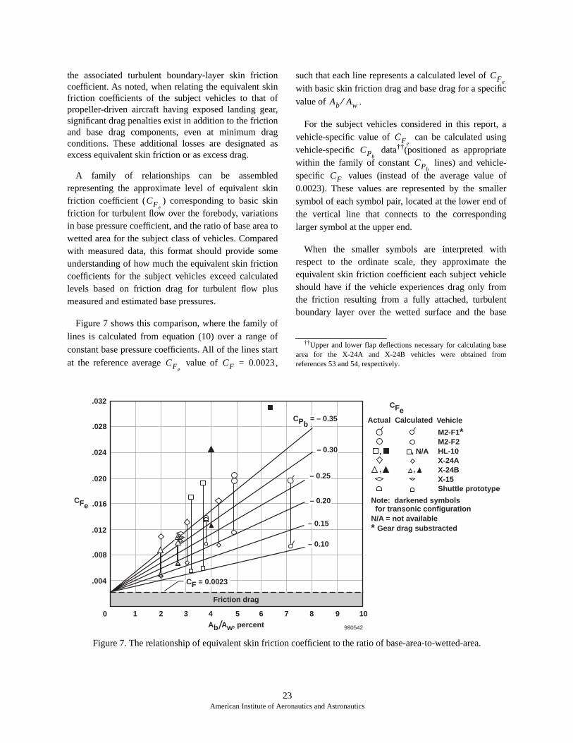
A family of relationships can be assembledrepresenting the approximate level of equivalent skinfriction coefficient ( ) corresponding to basic skinfriction for turbulent flow over the forebody, variationsin base pressure coefficient, and the ratio of base area towetted area for the subject class of vehicles. Comparedwith measured data, this format should provide someunderstanding of how much the equivalent skin frictioncoefficients for the subject vehicles exceed calculatedlevels based on friction drag for turbulent flow plusmeasured and estimated base pressures.

Figure 7 shows this comparison, where the family of

lines is calculated from equation (10) over a range of

constant base pressure coefficients. All of the lines start

at the reference average value of ,

such that each line represents a calculated level of

with basic skin friction drag and base drag for a specific

value of .

For the subject vehicles considered in this report, avehicle-specific value of can be calculated usingvehicle-specific data††(positioned as appropriatewithin the family of constant lines) and vehicle-specific values (instead of the average value of0.0023). These values are represented by the smallersymbol of each symbol pair, located at the lower end ofthe vertical line that connects to the correspondinglarger symbol at the upper end.

When the smaller symbols are interpreted withrespect to the ordinate scale, they approximate theequivalent skin friction coefficient each subject vehicleshould have if the vehicle experiences drag only fromthe friction resulting from a fully attached, turbulentboundary layer over the wetted surface and the base

CFe

CFeCF 0.0023=

††Upper and lower flap deflections necessary for calculating basearea for the X-24A and X-24B vehicles were obtained fromreferences 53 and 54, respectively.

CFe

Ab Aw⁄

CFeCPb

CPbCF

Figure 7. The relationship of equivalent skin friction coefficient to the ratio of base-area-to-wetted-area.

.032

.028

.024

.020

.016

.012

.008

.004

0 4 5 6 7 8 9 101 2 3Ab/Aw, percent

CFe

CFe

M2-F1*M2-F2HL-10X-24AX-24BX-15Shuttle prototype

VehicleActual Calculated

Note: darkened symbols for transonic configurationN/A = not available

980542

Friction drag

,

, ,

, N/A

* Gear drag substracted

CF = 0.0023

– 0.30

– 0.25

– 0.20

– 0.15

– 0.10

CPb = – 0.35


drag associated with the pressure coefficients indicatedin table 3. The larger symbol at the upper end of a givenvertical line is the experimentally measured value of

for that vehicle as obtained from table 3. Theincrement of represented by the length of thevertical line segment connecting a symbol pairquantifies the excess drag (that is, the amount that theactual drag exceeds the presumed or calculated drag atthese minimum drag conditions). The authors speculatethat the excess drag increments result from:

• local regions of separated flow upstream of basestations or any trailing edges.

• vortices generated by deflected control surfaces,body crossflow, and in some cases, unproductiveside loads generated by outboard vertical or cantedfins.

• roughness and protuberance effects.

• compressibility effects.

• data uncertainty (see the “Data Uncertainty”section).

For example, note the M2-F2 lifting body (thecircular symbol without a flag), which has a base-area-to-wetted-area ratio of 4.9 percent. If no excess dragsources existed for this vehicle, its calculated level of

, associated with the measured base pressurecoefficient of –0.209 plus friction drag, would be0.0117. However, the actual level of for the M2-F2vehicle, (the larger circular symbols) is approximately0.020. Apparently, this vehicle experiences significantexcess drag beyond the skin friction and base drag, evenat minimum drag conditions. The M2-F1 and HL-10vehicles experience even larger excess drag.

The X-24B lifting-body vehicle is represented by thetriangular symbols. Unfortunately, base pressuremeasurements were made for this vehicle only in thetransonic configuration, wherein the very large upperand lower flap deflections created a flared afterbody.55

The sum of the upper and lower flap deflections wasapproximately 68°; refer to the schematic of body-flapangles in Figure 1(i). These data (the darkened trianglesymbols) were obtained at a Mach number of 0.8,whereas the other X-24B data presented in this paperwere obtained at Mach 0.5 and Mach 0.6 with smallerflap deflections. The very large excess drag incrementnoted between the large and small darkened triangularsymbols shows the obvious effects of compressibility

and of the large flare angles that produce higher dragfrom both the windward surface and from reducedpressure on the leeward side.56

This result, obtained at Mach 0.8, is included with theother data representing lower Mach numbers because itprovides a base pressure coefficient reference datumthat is used for estimating base pressure coefficients forthe X-24A and the other X-24B data pairs. The majorportion of the base region for these two vehicles is thesame; and the upper and lower body flaps, whichinfluence the base area as they are deflected, areidentical. Note that the X-24B vehicle had a very largeincrement of excess drag for the transonic configuration(the darkened triangles) as would be expected; however,the X-24B subsonic configurations experienced excessdrag increments much smaller than those for the otherlifting bodies. The excess drag of the X-24A vehicle, atlow lift, is somewhat larger than that of the subsonicX-24B vehicle, but is still much smaller than those ofthe earlier lifting-body configurations (the M2-F1,M2-F2, and HL-10 vehicles).

The excess low-lift drag increment for the X-15aircraft is very small. The likely reason for this smallincrement is the relatively high-fineness ratio of thefuselage, thin wings, and horizontal stabilizer, whichallows for small-angle aft-sloping surfaces. Therefore,these surfaces maintain a proverse pressure gradient thatassures attached flow. These features virtuallyeliminated compressibility effects.

Because the Shuttle prototype Enterprise had aroughened surface to simulate the thermal protectionsystems of the actual orbiting Space Shuttles to follow,the value of used to determine the position of thesmaller symbol for the Shuttle prototype (fig. 7) is toolow for this vehicle. Consequently, the excess dragincrement shown for the Shuttle prototype in figure 7 istoo large, but the magnitude of this discrepancy cannotbe quantified based on the presently available data.‡‡

Base Pressure Coefficients

Hoerner compiled base pressure data from projectiles,fuselage shapes, and other small-scale three-dimensional shapes31 and derived therefrom an equation

CFeCFe

CFe

CFe

‡‡According to reference 57, preflight estimates of thermalprotection system drag indicated an additional increment of 0.00084(based on wetted area) to the Shuttle friction drag. However,reference 57 also considered the estimate of thermal protection systemdrag to be too large after examining postflight data from an orbitingSpace Shuttle (Columbia, mission STS-2).

CF


that related the base drag and base pressure coefficientsto the forebody drag of the respective bodies (eq. (14)).Reference 31 also includes an equation that describesthe analogous relationship for quasi-two-dimensionalshapes that shed vortices in a periodic manner, the well-known Kármán vortex street (eq. (15)). Base pressuredata from some of the subject vehicles will be comparedon the basis of the Hoerner relationships andmodifications to his equations (using differentK values). The search for flight-measured base pressuredata for the seven subject vehicles is somewhatdisappointing, considering that each of these vehicleshas a significant component of base drag. Table 4 showsthe results of the literature search.

Note that the M2-F3 vehicle is virtually the same asthe M2-F2 vehicle. All configurational dimensions arethe same except that a centerline upper vertical fin wasadded to the M2-F3 vehicle. For this reason, theunpublished base pressure data from the M2-F3 liftingbody are accepted as representative of those of theM2-F2 lifting body. Consequently, the M2-F2 and theM2-F3 lifting bodies will be treated as if they were thesame vehicle in the analysis to follow.

Because of Hoerner’s convincing demonstration thatbase pressure is related to forebody drag, comparing theavailable base pressure coefficients from the subjectvehicles to his equations is possible. Figure 8 showsthese comparisons. Figure 8 also includes a shaded bandfor Hoerner’s three-dimensional equation that isbounded by numerator coefficients, K, of 0.09 and 0.10.By modifying Hoerner’s original equation with theseK coefficients, the base pressure coefficients from theX-15, the M2-F3, and the Space Shuttle vehicles (which

are obviously three-dimensional) are observed to fallwithin or relatively close to this band.

Figure 8 also shows that the flight data are relativelyclose to Hoerner’s quasi-two-dimensional relationship(eq. (15)). The relatively higher (more negative)pressure coefficient from the X-24B vehicle (darktriangle) is caused by the large wedge angle, ahead ofthe base, formed by the upper and lower flaps that areused for control in pitch. The upper flap was deflectedupward approximately 40°, and the lower flap wasdeflected downward approximately 28°. This geometryis known to produce more negative base pressurecoefficients.56 The only base pressure data from theX-24B vehicle55 were unfortunately obtained with asignificantly larger wedge angle than existed for thesubsonic control configurations. The X-24B polars forMach 0.5 and Mach 0.6 were obtained using muchsmaller wedge angles.

The M2-F1 datum is unrepresentative of the subjectclass of vehicles in that the base region was pressurizedto some extent by turning vanes (one on each side,below the rudders). Based on the available flight data,the vehicles considered herein (excepting the M2-F1and the X-24B vehicles) are best represented by thethree-dimensional equation where – ,which means base drag of blunt-based large-scalevehicles is higher than predicted by Hoerner’s originalthree-dimensional equation. Based on evidence fromreferences 40 and 59 and figure 8, subsonic flowseparating from a relatively large, sharp-edged three-dimensional base can be argued to exhibit quasi-two-dimensional characteristics. In either case, the dataindicate more negative base pressure coefficients than

K 0.09= 0.10

Table 4. Base pressure sources.

Vehicle dataReferencenumber Remarks

M2-F1 Yes 10 The base region was pressurized by turning the vanes.

M2-F3 Yes Unpublished The M2-F3 data were applied to the M2-F2 vehicle.

HL-10 No The base drag data exist, but no explicit base pressure data exists.

X-24A No Base pressure coefficients were estimated using X-24B results.

X-24B Yes 55 Base pressure coefficients for Mach 0.5 and Mach 0.6 were estimated using Mach 0.8 results.

X-15 Yes 40

Space Shuttle Yes 58

CPb


the unmodified three-dimensional equation( ) would predict. Because of the large basedrag component these base pressures represent,employing a method of pressurizing the base regionmay be advisable. Such methods are available, althoughtheir use necessarily complicates the afterbody designdetails. Considering the very large losses caused by thebase region for this class of vehicles, such pressurizingdevices deserve attention.31, 60–66

Optimum Minimum Drag

Excluding the base pressure data from the M2-F1 andthe X-24B vehicles for the reasons already given, thedata from the other three vehicles (M2-F3, X-15, andSpace Shuttle vehicles) are believed to represent the

generic blunt-based class of vehicles. More large-scalebase pressure and overall minimum drag (and henceforebody drag) data must be obtained in flight toconvincingly demonstrate their relationship. Definingthis relationship for three or four values of forebodydrag for the same outer mold-line shape would be mosthelpful. Until more flight data are obtained or a superiorrelationship is developed, the shaded region of figure 8,derived from the data of the latter three vehicles, isassumed to be a reasonable representation of the basepressure characteristics for this class of reentry craft.Therefore, a revised version of Hoerner’s three-dimensional equation, , has been used toshow the dependence of minimum drag on the relativesize of the blunt base over a significant range of

K 0.029=

K 0.10=

Figure 8. Comparison of base pressure coefficients for subject vehicles with Hoerners’ two-dimensional relationshipand with revised three-dimensional equation.

M2-F1M2-F1M2-F3HL-10

X-24A

X-24B

X-24B

X-15Space Shuttle

Measured

MeasuredMeasured

MeasuredMeasuredMeasured

Forebody drag includes gear:Gear drag subtracted:Forebody drag from M2-F2CPb

derived from published base drag

CPb estimates based on X-24B,

CPb for transonic configuration, M = 0.8

CPb estimates based on X-24B,

– .6

– .5

– .4

– .3

– .2

Vehicle Remarks

turning vanespressurize base

CPbsource

– .1

0.03 .04 .06 .08 .10 .20 .30 .40 .60 .80 1.00

CPb

CDfore,b 980543

Equation (14)

– CPb =

K

CDfore,b

K = 0.100

K = 0.090

Equation (15), two-dimensional

K = 0.029

Forebody drag from Shuttle prototype


forebody drag. Figure 9 shows this illustration, whereeach of four curves shows how overall minimum dragcoefficient varies with forebody drag coefficient fordiscrete ratios of base area to wetted area (2.5, 5.0, 7.5,and 10 percent). The salient feature of these curves isthat each has an optimum region of lowest overallminimum drag coefficient, .

Note that for the 2.5-percent relationship, an optimumregion (a drag “bucket”) exists near the forebody dragcoefficient value of 0.003. Because these coefficients arebased upon the wetted area, and because the smoothskin turbulent friction coefficient for these Reynoldsnumbers (in the 107 to 108 range) would be close to0.002, a configuration having a base-area-to-wetted-arearelationship of 2.5 percent can afford only a minuteamount of roughness, protuberance, or separation dragover the forebody if the optimum is to be achieved.Conversely, for the higher base-area-to-wetted-arearelationships, which more closely represent manyreentry configurations, the optimum (or dragbucket) occurs at significantly higher values of forebodydrag coefficient, .

This characteristic should be of particular interestwith regard to some emerging reusable launch vehicles

that have relatively large base-area-to-wetted-area ratios(between 7.5 percent and 10 percent). This observation,of course, means that such configurations can afford (infact, may benefit from) additional forebody drag inaddition to the unavoidable smooth skin turbulentfriction. Thus, surface roughness that may accompany athermal protection system may actually provide areduction in overall while increasing the forebodydrag, providing the upper body is flat enough tomaintain attached, high-energy flow.

Such a reduction would be the result of forebodyroughness affecting the growth of the boundary layerfrom the nose to the edge of the base, which in turnaffects the level of “vacuum” or suction at the basethrough a “jet-pump mechanism” as described byHoerner.31 Thus, subject to the curves of figures 8 and 9,forebody roughness adds to the thickness of theboundary layer, thereby reducing the pumping(vacuuming) of the base and reducing the base drag. Thedrag bucket curves of figure 9 are related to those seenin chapters 6 and 13 of reference 31 for bodies, nacelles,canopies, and airfoils.

Figure 9 shows the relationship of to forebodydrag coefficient for the same vehicles as were

CFe

CFe

CFe

CFe′

CFe

CFe

Figure 9. The relationship of equivalent skin friction coefficients for the complete vehicle and the forebody.

.068

.060

.052

.044

.036

.028

.020

.012

.004

0 .004

3.8

2.72.0 2.7

2.0

3.1 4.3

4.0

3.77.2

3.44.9

3.2

.008 .012 .016 .020 .024

M2-F1M2-F2HL-10X-24AX-24BX-15

Shuttle prototype

Gear drag subtracted

, 68° wedge angle , 56° wedge angle, speed brakes

Vehicle Remarks

980544CFe

, forebody only´

2.8

Ab/Aw,

percent

2.5

5.0

7.5

10.0

Ab/Aw, percent

"Ideal" forebody drag coefficient, CFe

= CF´

CFe


represented in figure 8. The numbers adjacent to eachdata symbol indicate the base-area-to-wetted-area ratioof the respective vehicle at the specific flight condition.From these numbers, in relationship to the curves, notethat the data from the vehicles designated by the opensymbols (except the M2-F1 vehicle) are in qualitativeaccord with the semiempirical curves. As was statedearlier with regard to figure 8, overall for theM2-F1 vehicle is believed to be lower than thesemiempirical curves suggest because turning vanespressurized the base. For the X-24B vehicle (the darktriangle), the value of is believed to be highbecause of the aforementioned large flare angle thatlowers the lee-side pressures on the longitudinal controlbody flaps. This belief is not only supported by datafrom reference 56 but also by speed brake data from theX-15 aircraft (the dark symbol) which represent acomparable flared, or wedge, angle.67

The Effect of Fineness Ratio on Drag

Truncated or blunt-based bodies, such as the subjectvehicles, bear a familial relationship to the forward two-

thirds or three-fourths of a classical body of revolutionthat has a fully boat-tailed afterbody (for example,Sears-Haack). Considering whether the subsonicforebody drag of a blunt-based vehicle is dependent onfineness ratio, as is the drag of a fully boat-tailed body,is reasonable. To evaluate this relationship, the forebodydrag coefficients ( ) of the seven vehicles areplotted with respect to effective fineness ratio ( )in figure 10. The open symbols show a clear relationshipbetween forebody drag and fineness ratio, althoughconfigurational differences other than fineness ratio arelikely prominent for fineness ratios less than 3. As statedbefore for the discussion of figure 7, the solid trianglesymbol representing the X-24B vehicle shows a muchhigher forebody drag coefficient because of higherpressure on the windward surface of the body flaps,which are deflected to a large flare or wedge angle. TheX-15 forebody drag for partially deflected speed brakes(the solid diamond symbol) is included here because itlends credence to the X-24B data, and discussion ofsame, in that the X-24B body flaps and the X-15 speedbrakes experience related flow phenomenon.

CFe

CFe

CFe′

l deff⁄

Figure 10. The relationship of forebody equivalent skin friction coefficient with fineness ratio.

.020

.016

.012

.008

.004

01 2 3 4 5 6 7 8 9 10

l/deff

M2-F1M2-F2HL-10X-24AX-24BX-15

Shuttle prototype

Vehicle RemarksGear drag subtracted

, 68° wedge angle, 56° wedge angle, speed brakes

980545

CFe


Summary of Results

Flight-determined lift and drag characteristics fromseven blunt-based lifting-body and wing-body reentryconfigurations have been compared and related toseveral standards of aerodynamic efficiency. For lift-curve slope, limited comparisons are made with genericwind-tunnel model results and the theoreticalrelationships of Jones and Helmbold. A summary ofmajor results is as follows:

1. Base pressure coefficient data from the X-15, theM2-F3, and the Space Shuttle vehicles indicatethat Hoerner’s equation relating base pressure tothree-dimensional forebody drag requires a largernumerator coefficient in order to represent large-scale flight vehicles. A tentative range of values forthe numerator coefficient is from 0.09 to 0.10rather than 0.029, which is based on small-scalemodel data.

2. Evidence exists that subsonic flow separatingfrom a relatively large, sharp-edged three-dimensional base can exhibit quasi-two-dimensional characteristics and base pressurecoefficients.

3. The nature of the Hoerner base-pressure-toforebody-drag relationship (regardless of whetherhis three-dimensional or two-dimensional equationis used, or the numerator coefficient value) causesbase drag and forebody drag to combine to forman optimum minimum drag (a drag “bucket”) overa small range of forebody drag. The magnitude offorebody drag coefficient that defines the bucketdepends on the ratio of base area to wetted area ofthe respective vehicle. A vehicle having a largebase-area-to-wetted-area ratio and a relatively flatupper surface may benefit from surface roughnessdrag (associated perhaps with a thermal protectionsystem) at low lifting conditions; this combinationof features may provide some favorablecompensation for low-fineness-ratio vehicleshaving a relatively large base.

4. Conversely, a strong relationship between forebodydrag and fineness ratio (favoring, of course, thehigher fineness ratios) has been demonstrated toexist. This characteristic, in concert with thepossibility of achieving the aforementioned dragbucket, underlines the importance of obtainingmore large-scale free-flight base pressure andforebody drag data. Such an investigation shouldeither confirm the numerator coefficient bandsuggested herein for the three-dimensional

equations ( ), confirm or refutethe two-dimensional nature of the separating flow,or define a new superior relationship that willreliably define the nature of the drag bucket forgeneral application.

5. Minimum equivalent parasite drag area values forthe vehicles range from 6.5 ft2 to 164 ft2. Divisionof equivalent drag area by the associated wettedarea provided equivalent skin friction coefficientsranging from approximately 0.009 to 0.020,excluding the less efficient body-flapconfigurations (these coefficients include basedrag). These minimum equivalent skin frictionvalues range from 4 to slightly more than 8 timesthe skin friction drag for the attached turbulentboundary layer alone.

6. When the base drag coefficient is subtracted fromthe minimum equivalent friction coefficient(thereby defining forebody drag coefficient), aconsiderable increment of excess drag above thatwhich would be attributable to an attachedturbulent boundary-layer still exists for all of thevehicles except the X-15 aircraft. These equivalentskin friction coefficients, for forebodies, rangedfrom approximately 1.2 to approximately 6.6 timesthe skin friction drag for the attached turbulentboundary-layer alone. This extra increment ofequivalent friction drag, referred to as excess drag,is believed to result from the following:

• local regions of separated flow upstream ofbase stations or any trailing edges.

• vortices generated by deflected control surfaces,body crossflow, and in some cases, unproductivesideloads generated by the outboard fins.

• roughness and protuberance effects.

• compressibility effects.

7. Little order existed to the lift-curve slope datawhen lift coefficient was based on the referenceareas used in the reports from which the data wereobtained. Application of more representativereference areas (for five of the seven vehicles)and adjustment of the lift-curve slopes forcompressibility provided improved order to thedata. These data demonstrate that the choice of aphysically meaningful (representative) referencearea is of major importance.

8. The M2-F2 data demonstrate that the lift-curveslope of very-low-aspect-ratio lifting bodies can

K 0.09 to 0.10=


exceed the lift-curve slope values represented bythe relationships of Jones or Helmbold for aspectratios less than approximately 1. The M2-F2results are not believed to be an anomaly becausethey are afforded credence by generic modelresults as well as by generic leading-edge vortexlift data and crossflow lift data.

9. Excepting the M2-F1 and the HL-10 vehicles, theremaining five vehicles form an array (a band of

over a range of ) that should bea useful reference source against which to relatefuture reentry-type vehicles.

References

1National Advisory Committee for Aeronautics,NACA Conference on High-Speed Aerodynamics: ACompilation of the Papers Presented, NASATM-X-67369, 1958.

2Faget, Maxime A., Benjamine J. Garland, andJames J. Buglia, “Preliminary Studies of MannedSatellites—Wingless Configuration: Nonlifting,” NACAConference on High-Speed Aerodynamics: ACompilation of the Papers Presented, NASATM-X-67369, 1958, pp. 19–33.

3Wong, Thomas J., Charles A. Hermach, John O.Reller, Jr., and Bruce E. Tinling, “Preliminary Studiesof Manned Satellites—Wingless Configurations:Lifting Body,” NACA Conference on High-SpeedAerodynamics: A Compilation of the Papers Presented,NASA TM-X-67369, 1958, pp. 35–44.

4Becker, John V., “Preliminary Studies of MannedSatellites—Winged Configurations,” NACAConference on High-Speed Aerodynamics: ACompilation of the Papers Presented, NASATM-X-67369, 1958, pp. 45–57.

5Chapman, Dean R., “Study of Motion and Heatingfor Entry Into Planetary Atmospheres,” NACAConference on High-Speed Aerodynamics: ACompilation of the Papers Presented, NASATM-X-67369, 1958, pp. 1–17.

6Love, Eugene S., “Introductory Considerations ofManned Reentry Orbital Vehicles,” Joint Conference onLifting Manned Hypervelocity and Reentry Vehicles: ACompilation of the Papers Presented, NASATM-X-67563, 1960, pp. 39–54.

7Dennis, David H. and George G. Edwards, “TheAerodynamic Characteristics of Some Lifting Bodies,”

Joint Conference on Lifting Manned Hypervelocity andReentry Vehicles: A Compilation of the PapersPresented, NASA TM-X-67563, 1960, pp. 103–119.

8Paulson, John W., Robert E. Shanks, and Joseph L.Johnson, “Low-Speed Flight Characteristics of ReentryVehicles of the Glide-Landing Type,” Joint Conferenceon Lifting Manned Hypervelocity and Reentry Vehicles:A Compilation of the Papers Presented, NASATM-X-67563, 1960, pp. 329–344.

9Reed, R. Dale with Darlene Lister, Wingless Flight:The Lifting Body Story, NASA SP-4220, 1997.

10Horton, Victor W., Richard C. Eldredge, andRichard E. Klein, Flight-Determined Low-Speed Liftand Drag Characteristics of the Lightweight M2-F1Lifting Body, NASA TN-D-3021, 1965.

11Smith, Harriet J., Evaluation of the Lateral-Directional Stability and Control Characteristics of theLightweight M2-F1 Lifting Body at Low Speeds, NASATN-D-3022, 1965.

12Pyle, Jon S. and Robert H. Swanson, Lift and DragCharacteristics of the M2-F2 Lifting Body DuringSubsonic Gliding Flight, NASA TM-X-1431, 1967.

13Pyle, Jon S., Lift and Drag Characteristics of theHL-10 Lifting Body During Subsonic Gliding Flight,NASA TN-D-6263, 1971.

14Ash, Lawrence G., Flight Test and Wind TunnelPerformance Characteristics of the X-24A Lifting Body,FTC-TD-71-8, June 1972.

15United States Air Force, Comparison of Flight Testand Wind Tunnel Performance Characteristics of theX-24B Research Aircraft, AFFTC-TR-76-10, Apr.1976.

16Flight Test Results Pertaining to the SpaceShuttlecraft, NASA TM-X-2101, 1970.

17Aerodynamics of Hypersonic Lifting Vehicles,AGARD-CP-428, Apr. 1987.

18Kempel, Robert W., Weneth D. Painter, andMilton O. Thompson, Developing and Flight Testingthe HL-10 Lifting Body: A Precursor to the SpaceShuttle, NASA RP-1332, 1994.

19Matranga, Gene J., Analysis of X-15 LandingApproach and Flare Characteristics Determined Fromthe First 30 Flights, NASA TN-D-1057, 1961.

L D⁄( )max b2

Aw⁄


20Matranga, Gene J. and Neil A. Armstrong,Approach and Landing Investigation at Lift-DragRatios of 2 to 4 Utilizing a Straight-Wing FighterAirplane, NASA TM-X-31, 1959.

21Saltzman, Edwin J. and Darwin J. Garringer,Summary of Full-Scale Lift and Drag Characteristicsof the X-15 Airplane, NASA TN-D-3343, 1966.

22Thompson, Milton O., “Final Remarks and FuturePlans,” Flight Test Results Pertaining to the SpaceShuttlecraft, NASA TM-X-2101, 1970, pp. 147–151.

23United States Air Force, AFFTC Evaluation of theSpace Shuttle Orbiter and Carrier Aircraft: NASAApproach and Landing Test, AFFTC-TR-78-14,May 1978.

24Krienes, Klaus, The Elliptic Wing Based on thePotential Theory, NACA TM-971, 1941.

25Helmbold, H. B., “Der unverwundeneEllipsenflugel als tragende Flache,” Jahrb, 1942 derDeutschen Luftfahrtforschung, R. Oldenbourg(Munich), pp. I-111–I-113.

26Polhamus, Edward C., A Simple Method ofEstimating the Subsonic Lift and Damping in Roll ofSweptback Wings, NACA TN-1862, 1949.

27Jones, Robert T., Properties of Low-Aspect-RatioPointed Wings at Speeds Below and Above the Speed ofSound, NACA Report 835, 1946.

28Brown, Clinton E. and Michael, William H., Jr.,On Slender Delta Wings with Leading-EdgeSeparation, NACA TN-3430, 1955.

29Allen, H. Julian and Edward W. Perkins, A Study ofEffects of Viscosity on Flow Over Slender InclinedBodies of Revolution, NACA Report 1048, 1951.

30Hoerner, Sighard F. and Henry V. Borst, Fluid-Dynamic Lift: Practical Information on Aerodynamicand Hydrodynamic Lift, published by Liselotte A.Hoerner, 1985.

31Hoerner, Sighard F., Fluid-Dynamic Drag:Practical Information on Aerodynamic Drag andHydrodynamic Resistance, Published by the author,1965.

32Oswald, W. Bailey, General Formulas and Chartsfor the Calculation of Airplane Performance, NACAReport 408, 1932.

33Wendt, R. E., “A Method of Airplane PerformanceCalculation Applicable to Any Polar,” Journal of theAeronautical Sciences, vol. 14, no. 4, Apr. 1947,pp. 243–250.

34Raymer, Daniel P., Aircraft Design: A ConceptualApproach, AIAA Education Series, 1992.

35Stinton, Darrol, The Design of the Aeroplane, VanNostrand Rheinhold Company, New York, 1983.

36Loftin, Laurence K., Jr., Subsonic Aircraft:Evolution and the Matching of Size to Performance,NASA RP-1060, 1980.

37Perkins, Courtland D. and Robert E. Hage,Airplane Performance Stability and Control, JohnWiley and Sons, New York, 1949.

38Peterson, John B., Jr., A Comparison ofExperimental and Theoretical Results for theCompressible Turbulent-Boundary-Layer Skin FrictionWith Zero Pressure Gradient, NASA TN-D-1795, 1963.

39Bertram, Mitchel H., Calculations of CompressibleAverage Turbulent Skin Friction, NASA TR-R-123,1962.

40Saltzman, Edwin J., Base Pressure CoefficientsObtained From the X-15 Airplane for Mach Numbersup to 6, NASA TN-D-2420, 1964.

41Research-Airplane-Committee Report onConference on the Progress of the X-15 Project: ACompilation of the Papers Presented, NASATM-X-57072, 1961.

42Watts, Joe D. and Ronald P. Banas, X-15 StructuralTemperature Measurements and Calculations forFlights to Maximum Mach Numbers of Approximately4, 5, and 6, NASA TM-X-883, 1963.

43Gord, P. R., Measured and Calculated StructuralTemperature Data From Two X-15 Airplane FlightsWith Extreme Aerodynamic Heating Conditions, NASATM-X-1358, 1967.

44Pearson, Henry A. and Dorothy E. Beadle, FlightMeasurements by Various Methods of the DragCharacteristics of the XP-51 Airplane, NACAMR-L6F12, 1946.

45Beeler, De E., Donald R. Bellman, and Edwin J.Saltzman, Flight Techniques for Determining AirplaneDrag at High Mach Numbers, NACA TN-3821, 1956.


46Ware, George M., Low-Subsonic-Speed StaticStability of Right-Triangular-Pyramid and Half-ConeLifting Reentry Configurations, NASA TN-D-646,1961.

47Stivers, Louis S., Jr. and Lionel L. Levy, Jr.,Longitudinal Force and Moment Data at MachNumbers From 0.60 to 1.40 for a Family of EllipticCones With Various Semiapex Angles, NASATN-D-1149, 1961.

48Pyle, Jon S. and Lawrence C. Montoya, Effect ofRoughness of Simulated Ablated Material on Low-Speed Performance Characteristics of a Lifting-BodyVehicle, NASA TM-X-1810, 1969.

49Layton, Garrison P. Jr., Interim Results of theLifting-Body Flight-Test Program, NASA TM-X-1827,1969.

50Gothert, B., Plane and Three-Dimensional Flow atHigh Subsonic Speeds, NACA TM-1105, 1946.

51DeYoung, John and Charles W. Harper,“Theoretical Symmetric Span Loading at SubsonicSpeeds for Wings Having Arbitrary Plan Form,” Thirty-fourth Annual Report of the National AdvisoryCommittee for Aeronautics: 1948, 1951, pp. 593–648.

52Roskam, Jan, Airplane Design, Part VI:Preliminary Calculation of Aerodynamic, Thrust andPower Characteristics, Roskam Aviation andEngineering Corporation, Ottawa, Kansas, 1990.

53Hoey, Robert G., Flight Test Handling Qualities ofthe X-24A Lifting Body, FTC-TD-71-11, Feb. 1973.

54Nagy, Christopher J. and Paul W. Kirsten,Handling Qualities and Stability Derivatives of theX-24B Research Aircraft, AFFTC-TR-76-8, Mar. 1976.

55United States Air Force, Correlation of X-24BFlight and Wind Tunnel Pressure Data,AFFDL-TR-78-93, Sept. 1978.

56Butsko, J. E., W. V. Carter, and W. Herman,Development of Subsonic Base Pressure PredictionMethods, AFFDL-TR-65-157, vol. 1, Aug. 1965.

57Kirsten, Paul W., David F. Richardson, and CharlesM. Wilson, “Predicted and Flight Test Results of thePerformance, Stability and Control of the Space Shuttle

From Reentry to Landing,” Shuttle Performance:Lessons Learned, NASA CP-2283, part 1, 1983,pp. 509–524.

58Phillips, W. P., H. R. Compton, and J. T. Findlay,“Base Drag Determination for STS Flights 1–5,”AIAA-83-2719, Nov. 1983.

59Whitmore, Stephen A. and Timothy R. Moes,“Drag Measurements on the LASRE Flight Experimentand Their Relevance to the X-33,” AIAA-99-0277, tobe presented at the 37th AIAA Aerospace SciencesMeeting and Exhibit, Reno, Nevada, January 11–14,1999.

60Nash, J. F., A Discussion of Two-DimensionalTurbulent Base Flows, NPL Aero Report 1162, July1965.

61Pollock, N., Some Effects of Base Geometry onTwo Dimensional Base Drag at Subsonic andTransonic Speeds, Department of Supply, AustralianDefence Scientific Service Aeronautical ResearchLaboratories, Aerodynamics Note 316, Oct. 1969.

62Tanner, M., “Reduction of Base Drag,” ProgressiveAerospace Science, vol. 16, no. 4, 1975, pp. 369–384.

63Tanner, M., “A Method for Reducing the BaseDrag of Wings With Blunt Trailing Edge,”Aeronautical Quarterly, vol. 23, no. 1, Feb. 1972,pp. 15–23.

64Saltzman, Edwin J. and John Hintz, FlightEvaluation of Splitter-Plate Effectiveness in ReducingBase Drag at Mach Numbers From 0.65 to 0.90,NASA TM-X-1376, 1967.

65Tanner, Mauri, “New Investigations for Reducingthe Base Drag of Wings With a Blunt Trailing Edge,”Aerodynamic Drag, AGARD-CP-124, Apr. 1973,pp. 12-1–12-9.

66Pyle, Jon S. and Edwin J. Saltzman, “Review ofDrag Measurements From Flight Tests of MannedAircraft With Comparisons to Wind-TunnelPredictions,” Aerodynamic Drag, AGARD-CP-124,Apr. 1973, pp. 25-1–25-12.

67Saltzman, Edwin J., Preliminary Full-Scale Power-Off Drag of the X-15 Airplane for Mach Numbers From0.7 to 3.1, NASA TM-X-430, 1960.

REPORT DOCUMENTATION PAGE Form ApprovedOMB No. 0704-0188

Public reporting burden for this collection of information is estimated to average 1 hour per response, including the time for reviewing instructions, searching existing data sources, gathering andmaintaining the data needed, and completing and reviewing the collection of information. Send comments regarding this burden estimate or any other aspect of this collection of information,including suggestions for reducing this burden, to Washington Headquarters Services, Directorate for Information Operations and Reports, 1215 Jefferson Davis Highway, Suite 1204, Arlington,VA 22202-4302, and to the Office of Management and Budget, Paperwork Reduction Project (0704-0188), Washington, DC 20503.

1. AGENCY USE ONLY (Leave blank) 2. REPORT DATE 3. REPORT TYPE AND DATES COVERED

4. TITLE AND SUBTITLE 5. FUNDING NUMBERS

6. AUTHOR(S)

8. PERFORMING ORGANIZATION REPORT NUMBER

7. PERFORMING ORGANIZATION NAME(S) AND ADDRESS(ES)

9. SPONSORING/MONITORING AGENCY NAME(S) AND ADDRESS(ES) 10. SPONSORING/MONITORING AGENCY REPORT NUMBER

11. SUPPLEMENTARY NOTES

12a. DISTRIBUTION/AVAILABILITY STATEMENT 12b. DISTRIBUTION CODE

13. ABSTRACT (Maximum 200 words)

14. SUBJECT TERMS 15. NUMBER OF PAGES

16. PRICE CODE

17. SECURITY CLASSIFICATION OF REPORT

18. SECURITY CLASSIFICATION OF THIS PAGE

19. SECURITY CLASSIFICATION OF ABSTRACT

20. LIMITATION OF ABSTRACT

NSN 7540-01-280-5500 Standard Form 298 (Rev. 2-89)Prescribed by ANSI Std. Z39-18298-102

Flight-Determined Subsonic Lift and Drag Characteristics of SevenLifting-Body and Wing-Body Reentry Vehicle Configurations WithTruncated Bases

529-50-04-T2-RR-00-000

Edwin J. Saltzman, K. Charles Wang, and Kenneth W. Iliff.

NASA Dryden Flight Research CenterP.O. Box 273Edwards, California 93523-0273

H-2287

National Aeronautics and Space AdministrationWashington, DC 20546-0001 H-2287

This paper examines flight-measured subsonic lift and drag characteristics of seven lifting-body and wing-body reentry vehicle configurations with truncated bases. The seven vehicles are the full-scale M2-F1, M2-F2,HL-10, X-24A, X-24B, and X-15 vehicles and the Space Shuttle prototype. Lift and drag data of the variousvehicles are assembled under aerodynamic performance parameters and presented in several analytical andgraphical formats. These formats unify the data and allow a greater understanding than studying the vehiclesindividually allows. Lift-curve slope data are studied with respect to aspect ratio and related to generic wind-tunnel model data and to theory for low- aspect-ratio planforms. The proper definition of reference area wascritical for understanding and comparing the lift data. The drag components studied include minimum dragcoefficient, lift-related drag, maximum lift-to-drag ratio, and, where available, base pressure coefficients. Theeffects of fineness ratio on forebody drag were also considered. The influence of forebody drag on afterbody(base) drag at low lift is shown to be related to Hoerner’s compilation for body, airfoil, nacelle, and canopydrag. These analyses are intended to provide a useful analytical framework with which to compare and evaluatenew vehicle configurations of the same generic family.

Aerodynamics, Lifting bodies, Reentry vehicles, Reusable launch vehicles

A03

32

Unclassified Unclassified Unclassified Unlimited

January 1999 Conference Paper

Presented as AIAA 99-0383 at the 37th AIAA Aerospace Sciences Meeting and Exhibit, Reno, Nevada,January 11-14, 1999.

Unclassified—UnlimitedSubject Category 02, 15

flight-determined subsonic lift and drag … american institute of aeronautics and astronautics...

Documents