Flexible Signal Processing Algorithms for Wireless

Communications

by

Matthew Lee Welborn

B.S., United States Naval Academy (1989)

M.S., Virginia Polytechnic Institute and State University (1996)

Submitted to the Department of Electrical Engineering and Computer

Science

in partial ful�llment of the requirements for the degree of

Doctor of Philosophy in Electrical Engineering

at the

MASSACHUSETTS INSTITUTE OF TECHNOLOGY

June 2000

c Massachusetts Institute of Technology 2000. All rights reserved.

Author . . . . . . . . . . . . . . . . . . . . . . . . . . . . . . . . . . . . . . . . . . . . . . . . . . . . . . . . . . . . . .

Department of Electrical Engineering and Computer Science

May 10, 2000

Certi�ed by. . . . . . . . . . . . . . . . . . . . . . . . . . . . . . . . . . . . . . . . . . . . . . . . . . . . . . . . . .

John V. Guttag

Professor and Department Head, Electrical Engineering and

Computer Science

Thesis Supervisor

Accepted by . . . . . . . . . . . . . . . . . . . . . . . . . . . . . . . . . . . . . . . . . . . . . . . . . . . . . . . . .

Arthur C. Smith

Chairman, Department Committee on Graduate Students

Flexible Signal Processing Algorithms for Wireless

Communications

by

Matthew Lee Welborn

Submitted to the Department of Electrical Engineering and Computer Science

on May 10, 2000, in partial ful�llment of the

requirements for the degree of

Doctor of Philosophy in Electrical Engineering

Abstract

Wireless communications systems of the future will experience more dynamic channel

conditions and a wider range of application requirements than systems of today. Such

systems will require exible signal processing algorithms that can exploit wireless

channel conditions and knowledge of end-to-end user requirements to provide e�cient

communications services.

In this thesis, we investigate wireless communications systems in which the sig-

nal processing algorithms are speci�cally designed to provide e�cient and exible

end-to-end functionality. We describe a design approach for exible algorithms that

begins with the identi�cation of speci�c modes of exibility that enable e�cient over-

all system operation. The approach then uses explicit knowledge of the relationships

between the input and output samples to develop e�cient algorithms that provide the

desired exible behavior. Using this approach, we have designed a suite of novel algo-

rithms for essential physical layer functions. These algorithms provide both dynamic

functionality and e�cient computational performance.

We present a new technique that directly synthesizes digital waveforms from pre-

computed samples, a matched �lter detector that uses multiple threshold tests to

provide e�cient and controlled performance under variable noise conditions, and a

novel approach to narrowband channel �ltering. The computational complexity of the

�ltering algorithm depends only on the output sample rate and the level of interference

present in the wideband input signal. This is contrast to conventional approaches,

where the complexity depends upon the input sample rate. This is achieved using

a composite digital �lter that performs e�cient frequency translation and a tech-

nique to control the channel �lter output quality while reducing its computational

requirements through random sub-sampling.

Finally, we describe an implementation of these algorithms in a software radio

system as part of the SpectrumWare Project at MIT.

Thesis Supervisor: John V. Guttag

Title: Professor and Department Head, Electrical Engineering and Computer Science

Acknowledgments

I wish to thank my advisor, John Guttag, for his encouragement, ideas and support

in bringing this work to fruition.

I am grateful to all of my present and former colleagues in the Software Devices

and Systems Group for their help and ideas throughout the course of my work. My

work builds upon the work of many others, including Vanu Bose and Mike Ismert.

I am particularly grateful to John Ankcorn for his helpful insights and feedback on

many di�erent aspects of this work, and even for all of his questions that led me to

think about parts of this work in new ways.

Some of this work was done in conjunction with David Karger and Rudi Seitz, who

have helped me to learn a little bit more about how computer scientists think and

solve problems. I hope that they have also learned a little bit about signal processing.

I would also like to acknowledge the support of the National Science Foundation

through a graduate research fellowship that has made much of my graduate studies

possible.

Finally, I am forever grateful to my loving wife and children for their understanding

and support during these years that we have spent at MIT, and especially to my Lord

Jesus Christ who has blessed me with such a wonderful family and so many rewarding

opportunities.

Contents

1 Introduction 15

2 Flexible Design of Wireless Systems 23

2.1 Signal processing in the Physical Layer . . . . . . . . . . . . . . . . . 23

2.2 E�ects of Mobility on the Wireless Channel . . . . . . . . . . . . . . 25

2.2.1 Propagation characteristics and capacity . . . . . . . . . . . . 25

2.2.2 Dynamic conditions . . . . . . . . . . . . . . . . . . . . . . . . 27

2.3 E�ects of Diverse Communications Services . . . . . . . . . . . . . . 28

2.4 Design of Wireless Communications Systems . . . . . . . . . . . . . . 28

3 Balancing Flexibility and Performance 31

3.1 Key Elements for Flexible Algorithm Design . . . . . . . . . . . . . . 32

3.1.1 Flexibility to support function and performance . . . . . . . . 32

3.1.2 Understanding explicit data dependencies . . . . . . . . . . . 33

3.1.3 Techniques for e�ciency with exibility . . . . . . . . . . . . . 34

3.2 Related Work . . . . . . . . . . . . . . . . . . . . . . . . . . . . . . . 35

4 Flexible Processing in a Digital Transmitter 39

4.1 Overview: The Digital Modulator . . . . . . . . . . . . . . . . . . . . 40

4.2 Conventional Digital Waveform Generation . . . . . . . . . . . . . . . 42

4.2.1 Conventional techniques for digital modulation . . . . . . . . . 43

4.2.2 Direct digital synthesis of a sinusoidal carrier signal . . . . . . 46

4.3 Direct Waveform Synthesis for Modulation . . . . . . . . . . . . . . . 47

4.3.1 A new approach to modulation: Direct mapping . . . . . . . . 48

4.3.2 Decomposing tables to reduce memory . . . . . . . . . . . . . 51

4.3.3 Extensions of direct waveform synthesis . . . . . . . . . . . . . 52

4.4 Performance and Resource Trade-o�s . . . . . . . . . . . . . . . . . . 54

4.4.1 Performance comparison . . . . . . . . . . . . . . . . . . . . . 54

4.4.2 Memory versus computation . . . . . . . . . . . . . . . . . . . 56

4.5 Empirical Performance Evaluation . . . . . . . . . . . . . . . . . . . . 58

4.6 Implementation of a DWS Modulator . . . . . . . . . . . . . . . . . . 59

4.7 Summary . . . . . . . . . . . . . . . . . . . . . . . . . . . . . . . . . 59

7

8 CONTENTS

5 Flexible Processing in a Digital Receiver 63

5.1 Overview: Channel Separation . . . . . . . . . . . . . . . . . . . . . . 64

5.2 Conventional Approaches to Channel Separation . . . . . . . . . . . . 68

5.3 A New Approach to Frequency Translation . . . . . . . . . . . . . . . 71

5.3.1 Implementation of a narrowband �ltering system . . . . . . . 73

5.4 A New Approach to Bandwidth Reduction . . . . . . . . . . . . . . . 73

5.4.1 Decoupling �lter length and SNR . . . . . . . . . . . . . . . . 74

5.4.2 Random sub-sampling . . . . . . . . . . . . . . . . . . . . . . 76

5.4.3 Model for analysis . . . . . . . . . . . . . . . . . . . . . . . . 78

5.4.4 Analytical evaluation of the sequence transformer . . . . . . . 89

5.5 Evaluation of Random Sub-sampling . . . . . . . . . . . . . . . . . . 92

5.6 Summary . . . . . . . . . . . . . . . . . . . . . . . . . . . . . . . . . 96

6 Data Symbol Detection 97

6.1 Overview: Symbol Detection . . . . . . . . . . . . . . . . . . . . . . . 97

6.2 Conventional Approach to Detection . . . . . . . . . . . . . . . . . . 99

6.2.1 The design of pulses for digital modulation . . . . . . . . . . . 100

6.2.2 The matched �lter detector . . . . . . . . . . . . . . . . . . . 102

6.3 E�cient Detection for Error Control . . . . . . . . . . . . . . . . . . 105

6.3.1 A general framework for detection . . . . . . . . . . . . . . . . 105

6.4 Detection for Controlled Error Probability . . . . . . . . . . . . . . . 108

6.4.1 Data-e�cient decisions . . . . . . . . . . . . . . . . . . . . . . 108

6.4.2 A generalized threshold test . . . . . . . . . . . . . . . . . . . 111

6.4.3 Detection using multiple tests . . . . . . . . . . . . . . . . . . 112

6.5 Performance of a two-test detector . . . . . . . . . . . . . . . . . . . 116

6.6 Summary . . . . . . . . . . . . . . . . . . . . . . . . . . . . . . . . . 122

7 Summary, Contributions and Future Work 123

7.1 Contributions . . . . . . . . . . . . . . . . . . . . . . . . . . . . . . . 124

7.2 Future Work . . . . . . . . . . . . . . . . . . . . . . . . . . . . . . . . 126

7.2.1 Investigation of Additional Physical Layer Functions . . . . . 126

7.2.2 Flexible System Design . . . . . . . . . . . . . . . . . . . . . . 126

7.3 Conclusions . . . . . . . . . . . . . . . . . . . . . . . . . . . . . . . . 127

List of Figures

2-1 A wireless communications system. . . . . . . . . . . . . . . . . . . . 24

3-1 Performance pro�les for (a) a conventional algorithm and (b) anytime

algorithm (adapted from [Zilberstein, 1996]). . . . . . . . . . . . . . . 36

4-1 Stages of processing within the Channel Encoder . . . . . . . . . . . 39

4-2 Typical modulation techniques for encoding bits into a continuous

waveform: (a) amplitude modulation, (b) frequency modulation, and

(c) phase modulation. . . . . . . . . . . . . . . . . . . . . . . . . . . . 41

4-3 Two symbol constellations used to map blocks of four bits into complex

symbols for PAM, commonly known as (a) 16-QAM and (b) 16-PSK. 44

4-4 Conventional QAM modulator . . . . . . . . . . . . . . . . . . . . . . 45

4-5 Typical sin(x)=x pulse shape for a bandwidth-e�cient system, where

x = �t=T and T is the symbol interval. . . . . . . . . . . . . . . . . . 48

4-6 Proposed QAM modulator . . . . . . . . . . . . . . . . . . . . . . . . 49

4-7 Section of a synthesized 4-PAM waveform with Ns = 8 samples per

symbol interval. Individual table entries are indicated by boxes. . . . 50

4-8 QAM modulator using parallel look-ups to reduce table size. . . . . . 52

4-9 Plots showing memory requirements versus number of symbol periods

per table entry for (a) 8-PAM and (b) 16-QAM waveform synthesis

with K = 6, Ns = 10. . . . . . . . . . . . . . . . . . . . . . . . . . . . 57

4-10 Graphical user interface for an implementation of a direct waveform

synthesis digital modulator. . . . . . . . . . . . . . . . . . . . . . . . 60

4-11 Received signal constellation diagrams for (a) 8-PSK under relatively

high SNR (b) 8-PSK under low SNR and (c) 4-PSK under low SNR. . 61

5-1 Required processing steps in a digital receiver. . . . . . . . . . . . . . 63

5-2 Typical processing for narrowband channel selection. . . . . . . . . . 66

5-3 Conceptual steps used for conventional approach to narrowband chan-

nel selection: (a) frequency translation, (b) bandwidth reduction, and

(c) sample rate reduction. . . . . . . . . . . . . . . . . . . . . . . . . 67

9

10 LIST OF FIGURES

5-4 Block diagram showing frequency translation of desired signal before

�ltering and decimation. . . . . . . . . . . . . . . . . . . . . . . . . . 68

5-5 Block diagram showing (a) frequency translation of desired signal be-

fore �ltering and decimation, and (b) new approach that uses a com-

posite �lter to reduce computation. . . . . . . . . . . . . . . . . . . . 71

5-6 Illustration of how we decouple the length of the �lter input region

from the number of samples that it contains. . . . . . . . . . . . . . 75

5-7 Diagram showing conventional FIR �lter and model for approximating

output samples. . . . . . . . . . . . . . . . . . . . . . . . . . . . . . . 78

5-8 Distortion due to discarding input samples according to random coin

ips. . . . . . . . . . . . . . . . . . . . . . . . . . . . . . . . . . . . . 81

5-9 Model for analysis of error variance due to random sub-sampling. . . 82

5-10 Random sub-sampling using a transformed sequence for sample selection. 85

5-11 Output error variance relative to desired signal power versus propor-

tion of input samples used for several cases of output signal relative

bandwidth. . . . . . . . . . . . . . . . . . . . . . . . . . . . . . . . . 93

5-12 Comparison of Case I and Case II results for three values of var(xn). 95

6-1 Diagram of the channel decoder showing division of the symbol detector

into synchronization and detection steps. . . . . . . . . . . . . . . . . 98

6-2 Plot of bit-error rate versus SNR for a two level PAM system. . . . . 99

6-3 Representation of (a) an isolated pulse satisfying the zero ISI condition,

(b) multiple scaled and shifted pulses and (c) the noise-free composite

waveform. (In the plots, T = Tb, the symbol interval.) . . . . . . . . . 101

6-4 Cascade of transmit pulse-shaping �lter and receive �lter whose com-

bined response satis�es the Nyquist Criterion for zero ISI. . . . . . . 103

6-5 Projection of noisy received vector onto the line connecting the two

possible transmitted points. . . . . . . . . . . . . . . . . . . . . . . . 104

6-6 Conditional PDFs for H=0 and H=1. . . . . . . . . . . . . . . . . . . 105

6-7 Footprints of symbols within the sample sequence. . . . . . . . . . . . 107

6-8 Conditional PDFs for Un conditioned on H = 1 for several values of n,

where n1 < n2 < n3. . . . . . . . . . . . . . . . . . . . . . . . . . . . 110

6-9 Conditional PDFs for H = 0 and H = 1 and the three decision regions

de�ned by: (un < (�T )), (�T < uN < T ), and (T < uN). . . . . . . . 112

6-10 Plot of the six di�erent regions for the di�erent combination of out-

comes of the two tests in the S1-S2 plane. . . . . . . . . . . . . . . . . 115

6-11 Plots of raised cosine and rectangular pulses (a) time domain and (b)

cumulative energy in sorted samples. . . . . . . . . . . . . . . . . . . 117

6-12 Plot of BER versus number of samples used in decision for various

levels of SNR. . . . . . . . . . . . . . . . . . . . . . . . . . . . . . . . 118

LIST OF FIGURES 11

6-13 Modi�ed performance curve for binary detection using minimum num-

ber of samples to achieve bounded BER. . . . . . . . . . . . . . . . . 119

6-14 Lowest threshold value for potential values of ki. . . . . . . . . . . . 120

6-15 Expected number of samples required for each bit decision using a

two-test detector. . . . . . . . . . . . . . . . . . . . . . . . . . . . . 121

12 LIST OF FIGURES

List of Tables

4.1 Required operations for conventional QAM modulator . . . . . . . . . 55

4.2 Required operations for proposed DWS modulator . . . . . . . . . . . 55

4.3 Results of software implementations of conventional QAM modulator

and DWS modulator. . . . . . . . . . . . . . . . . . . . . . . . . . . . 58

13

14 LIST OF TABLES

Chapter 1

Introduction

Communications- anytime, anywhere. This mantra is often repeated as designers and

producers of communications networks advertise new capabilities and services avail-

able because of recent technological developments. Indeed, with the proper equip-

ment, we can communicate voice, data and images anywhere in the world (or out

of it). An important part of this universal communications network will, of course,

be the portions that provide mobility and access to the global infrastructure with-

out wires. Today, it is this wireless portion of the system that seems to lag behind

expectations.

To be sure, wireless communications systems have changed signi�cantly in the past

ten years. Most notable, of course, is the sheer number of people that use wireless

communications services today. This trend of increased usage is expected to continue

and has generated considerable activity in the area of communications system design.

Another clear trend has been the type of information that these wireless systems

convey: virtually all new wireless systems are digital communications systems; unlike

earlier broadcast and cellular systems, newer systems communicate using digital data

encoded into radio waves. Even analog source information such as voice and images

are digitized and then transmitted using digital formats.

The reasons for this shift to digital wireless systems are several. Initially, the shift

was made in cellular telephone systems to improve system capacity through more

e�cient usage of the limited radio frequency (RF) spectrum. This shift has also

made available more advanced features, better performance, and more security for

users. Another reason for the shift in future systems, however, will be the fact that

almost all information communicated through such systems will already be digital,

both between individual users and between computers.

This shift toward digitizing all information for transmission does not mean that

all data should be treated as equivalent. Another trend in future wireless communi-

cations should be di�erentiated support for heterogeneous tra�c, such as voice, data

15

16 CHAPTER 1. INTRODUCTION

and video. Di�erent types of data tra�c will have varying requirements for transmis-

sion through the communications system, including di�erent requirements for latency,

error performance and overall data rate.

At the same time that usage becomes more widespread, users will also desire bet-

ter performance: not only higher data rates for future applications, but also better

reliability and coverage. In fact, users will want these systems to work as well as

conventional wire-line systems, just without the wires. The desire for wireless con-

nectivity will include not only increased total area of coverage, but also the ability

to transparently move within zones, maintaining reliable connectivity using light-

weight, low-power communication devices. This will lead to a wider range of oper-

ating conditions within the wireless channel due to mobility and the requirement for

communications services in diverse environments.

In order to meets these demands and ful�ll the vision of universal connectivity,

wireless systems of the future will have to provide a level of exible and e�cient service

not seen in current systems. These systems will have to carefully manage limited

resources such as spectrum and power as they provide services and performance far

superior to any available today. Furthermore, this increased exibility will have to

extend to those layers of the system that interface with the wireless channel: the

physical layer.

The algorithms that perform the processing in this layer are directly impacted by

the dynamic conditions and increased demands for e�ciency and performance implied

by the trends above. These algorithms will have to provide exibility in the way that

they accomplish their work under changing conditions in the wireless channel, yet

they will have to do this in a way that provides e�cient use of power exceeding the

best systems of today. In this work, we demonstrate that it is possible to design

algorithms that provide both exibility and e�ciency to meet the challenges that lie

ahead.

Summary and Interpretation of Contributions

In today's wireless communications systems, the physical layer processing is typically

implemented as a static design, providing an abstract interface to the upper layers

of the system as simply a bit transmission medium with some level of uncertainty at

the destination. Fixed hardware implementations reinforce this view of the physical

layer as immutable.

In this work, we consider the implication of recent technological advances that

make it possible for large portions of the physical layer processing to be implemented

in software [Mitola, 1995]. This shift leads us to consider designing communications

systems in which the physical layer implementation can be signi�cantly modi�ed in

response to changes in the operating environment or the needs of the end applica-

17

tions and users. A major conclusion of this thesis is that through careful design, we

can produce exible signal processing algorithms that enable the overall system to

e�ciently respond to such changes.

An important part of this work has been the implementation of many of the

resulting algorithms in a prototype wireless system. These implementations have

helped not only to validate the results, but have also helped to shape and guide

the research itself by providing a sense of the important problems and opportunities

for further investigation. Together, these goals of understanding how to best design

and implement a wireless communication system in which the physical layer can be

controlled in response to dynamic conditions and requirements has led to a number

of signi�cant results. The original contributions can be classi�ed into two separate

categories:

1. Novel signal processing algorithms that provide both exibility and improved

e�ciency relative to conventional techniques.

2. A new approach to designing exible signal processing algorithms.

We describe these two areas of contribution in more detail in the sections that follow.

Speci�c exible signal processing algorithms

Novel algorithms developed in this work perform functions that are required in several

di�erent parts of a wireless communications system. The �rst algorithm described

below is applicable to a digital wireless transmitter; the rest perform several of the

primary functions required in a digital wireless receiver:

Digital Modulation: We have developed a new approach for digital modula-

tion called direct waveform synthesis. This is a technique for mapping discrete

data for transmission into corresponding segments of a digitally modulated

waveform using a pre-computed table of samples. This approach is useful in

hardware and software implementations, providing computational advantages

of 20� relative to conventional techniques for modulation.

In the receiver, we divide our examination into two di�erent areas: the functions of

channel separation (isolating the desired signal) and detection, the process of recov-

ering the original transmitted data from the channel waveform.

Channel Separation: In this stage of processing, the receiver has to isolate

the desired narrow-band signal from a wideband input signal. This processing

typically has a computational complexity that is proportional to the bandwidth

of the input signal. We demonstrate new techniques that remove this depen-

dence, allowing the wideband receiver to be scaled to wider input bandwidths.

18 CHAPTER 1. INTRODUCTION

{ The frequency shifting �lter provides exible and e�cient frequency trans-

lation with a computational complexity proportional to the output sample

rate of the channel �lter. The computation relative to conventional tech-

niques is reduced by a factor equal to the ratio between input and output

bandwidths of the channel separator, which can be several hundred or more

in modern wideband receivers.

{ The channel separation process is computed using random sub-sampling of

discrete waveforms to enable e�cient �ltering. This new new approach uses

only a subset of the available input samples while maintaining controlled

signal-to-noise levels at the output. The computational complexity is again

decoupled from the input sample rate, and depends instead on the required

output signal quality.

Detection: To complete the process of recovering data, we present a multi-

threshold matched �lter detector that can provide a more e�ective balance be-

tween computation and the output con�dence levels needed for e�cient overall

system performance. Computational reductions of �ve or ten fold are demon-

strated relative to a full matched �lter detector, depending on the required

output quality and input noise levels.

Designing exible signal processing algorithms

In the design of a signal processing algorithm, a typical goal is to produce an algorithm

that can compute a speci�c result using some minimum amount of computation. From

a systems perspective, however, it is appropriate to design algorithms that can help

provide e�ciency in the context of the entire communications system. This approach

is especially important in the case of systems that will be expected to provide di�erent

services in a wide range of operating conditions.

Several common themes emerged from this work that have proven useful in produc-

ing e�cient, exible algorithms. These themes can be viewed as a general approach to

the development of e�ective signal processing algorithms in a larger communications

system. The steps of this approach are:

(1) Identify speci�c modes of exibility that are useful in providing overall system

e�ciency.

(2) Identify explicit relationships between input and output data samples for each

processing function, and

(3) E�ciently develop algorithms using the results of (1) and (2) through the re-

moval of unnecessary intermediate processing steps and the use of other tech-

19

niques borrowed from other disciplines, e.g. approximate and randomized algo-

rithms.

We must identify speci�cmodes of exibility needed for the overall communications

system to adapt to changing conditions. We can also typically improve performance

by eliminating types of exibility that are unnecessary for e�cient global adaptation.

An example of this is the matched �lter detector described above. Because of mobility

and dynamic channel conditions, the receiver often experiences varying levels of signal-

to-noise ratio (SNR). In the context of the entire system it is desirable for the detector

to produce constant quality output (measured as bit-error rate) in the presence of

variable input signal quality. In Chapter 6, we demonstrate a detector that can do

this e�ciently by reducing its computation under favorable SNR conditions.

We need a more explicit understanding of the input to output data relationships

for speci�c functions. To achieve the goal of exibility with e�ciency, it is important

to understand which speci�c input samples are relevant to the computation of a

particular output value, as well as their relative importance. In the channel separation

process discussed in Chapter 5, this understanding leads us to decouple the length of

a �lter response from the number of samples that are used to compute the output

value. In the case of the detector from Chapter 6, this knowledge enables us identify

the set of samples that contain information about speci�c bits to be estimated, and to

to preferentially process those input samples that contribute most to a useful result.

The �nal development step combines the understanding of the data relationships

and the targeted modes of exibility. In some cases, the role of a particular processing

function within the overall system enables a designer to specify a minimum level of

quality that is suitable for e�cient global operation under current conditions. An ap-

proach that provides the ability to simply approximate a more optimal computation

in a exible way might then lead to more e�cient algorithm. Because of the inherent

statistical properties of noisy signals, we found that it is useful in such cases to apply

techniques that provide statistical, rather than deterministic, performance guarantees

as a way to achieve more e�cient resource usage for desired levels of output qual-

ity. This is true for the detector described above and for the random sub-sampling

scheme that approximates the output of the channel separation �lter using statistical

techniques.

In other cases, where approximations to ideal output values are not appropriate,

it is often possible to use the explicit data relationships to provide improved e�-

ciency. In Chapters 4 and 5, we describe digital modulation and frequency transla-

tion approaches that produce results identical to conventional approaches while using

signi�cantly less computation. In these cases, understanding data relationships en-

abled the removal of unnecessary computation steps and the creation of more e�cient

algorithms without sacri�cing any useful modes of exibility.

20 CHAPTER 1. INTRODUCTION

Structure of this Thesis

Future wireless system designs will need to provide exible and e�cient service in

the face of more dynamic channel conditions and varying performance demands due to

heterogeneous tra�c. We claim that an approach that provides dynamic speci�cation

of physical layer signal processing functionality can satisfy these demands and meet

the end-to-end needs of the users. Because this thesis focuses on the processing

required in the physical layer of the communications system, Chapter 2 provides a

review of the relevant characteristics of the wireless channel and their implications in

light of the trends for future systems.

We present a discussion of a general design approach for exible and e�cient sig-

nal processing algorithms in Chapter 3, highlighting some of the common themes that

run throughout this work. The approach we describe begins with an understanding of

the speci�c modes of exibility that will be required in each stage of processing. We

also describe how a clear understanding of the relationships between the input and

output samples of a signal processing function is essential to the design of exible,

e�cient algorithms. The design approach then concludes by using the exibility goals

and data relationships to produce e�cient algorithms using a number of techniques

from the �eld of computer science. In this work, these techniques include the use

of random sub-sampling, functional composition for e�cient computation and condi-

tional termination of processing to reduce computation. In addition, the exible use

of look-up table based mapping enables a trade-o� between memory and computa-

tion. These design techniques are used in conjunction with the abstract processing

speci�cations and analysis tools of signal processing to produce exible algorithms.

In Chapter 4 we begin to describe the speci�c algorithms developed for signal

processing functions, starting with the transmitter. The processing required to encode

digital information into waveforms can be viewed as a direct mapping of data bits

into sequences of output samples. This understanding leads us to a exible look-up

table based approach that provides a wide choice of trade-o�s between memory and

computation in an e�cient digital modulator implementation, and we demonstrate

the signi�cant performance gains of this approach relative to conventional modulation

techniques.

We also describe the implementation of our digital modulation techniques in a

software radio system that was designed and built as part of the SpectrumWare

Project. This project has resulted in a number of applications that demonstrate the

utility of exible physical layer processing. Some of these applications are described

in both Chapters 4 and 5.

In Chapter 5, we begin discussion of the digital receiver with the problem of sep-

arating a narrowband channel from a wideband digital sample stream. This channel

separation task consists of two distinct steps: frequency translation and bandwidth

21

reduction. The �rst algorithm presented is a composite digital �lter that performs

part of the frequency translation step as the channel �lter output is computed. This

results in a signi�cant reduction in the computation required for the frequency trans-

lation step of channel separation.

We then present an approach to the bandwidth reduction step that is designed to

balance the output precision needs of the overall system with the desire to minimize

computational complexity. The key idea is to compute the output of the channel

�lter using only a subset of the available input samples. We describe algorithms

for choosing this subset of input samples in a non-deterministic manner to prevent

narrowband aliasing while carefully controlling the signal-to-noise ratio at the output

of the channel �lter.

One of the signi�cant results of Chapter 5 is that the computational complexity of

the channel separation function need not depend on the input sample rate. Instead,

we demonstrate that the channel separation function can be implemented with a

complexity that depends on the output sample rate and the level of interfering signals

are present in the wideband input signal at the time the algorithm is run.

Another essential function of a digital receiver is detection, where an estimate is

made of the original transmitted data based on the samples of the received signal.

In Chapter 6, we describe a new approach to detection, where the goal will be to

produce estimates with a bounded probability of error using minimum computation.

We present an algorithm that can produce such estimates with signi�cantly reduced

computation relative to conventional detection techniques. These performance gains

result from two distinct improvements, both of which involve the evaluation of only

a subset of the relevant samples for each data symbol estimate. For typical pulse

shapes used to transmit data, there is an uneven distribution of signal energy over

the duration of the pulse. We demonstrate that a signi�cant reduction in computa-

tion is possible with little e�ect on error probability by preferentially analyzing only

those samples that contain the most signal energy. Further performance gains are

then achieved through the introduction of a conditional test that enables the detec-

tion process to terminate early under favorable conditions, resulting is a detection

algorithm that has a statistical running time.

Finally, Chapter 7 summarizes the main contributions and themes of this work

and indicates some directions for future work. A review and discussion of related

work is presented in various places throughout the thesis.

22 CHAPTER 1. INTRODUCTION

Chapter 2

Flexible Design of Wireless

Systems

Communication is the transfer of information from the source to the destination. In

this process, resources are consumed: electrical power, RF spectrum, computational

resources or elapsed time. In this chapter, we review how future trends will make

it more challenging for mobile wireless systems to accomplish their communications

objectives while e�ciently using their limited resources.

We begin with a review of some of the functions to be performed in the physi-

cal layer processing for a wireless communications system and some of the relevant

characteristics of the RF wireless channel. We then describe how decisions about

the allocation of system resources impact the ability of the system to be exible and

e�cient. In particular, we will show that a static allocation of system resources to

individual users and a static design of the individual wireless links will result in un-

acceptable levels of ine�ciency. It is this need for an adaptive, exible physical layer

implementation that motivates the work in this thesis.

2.1 Signal processing in the Physical Layer

The physical layer provides the interface between the higher layers of the system

and the underlying physical communications medium, the analog wireless channel.

Processing steps required in the physical layer are shown in Figure 2-1.

Processing in this layer has long been referred to as signal processing because

it has involved continuous signals instead of discrete data. In the transmitter, the

modulation process transforms digital information into continuous signals appropriate

for the wireless channel. Because the wireless channel is a shared medium, the receiver

performs functions that provide for signal isolation in addition to demodulation. After

23

24 CHAPTER 2. FLEXIBLE DESIGN OF WIRELESS SYSTEMS

ErrorDecoder

SignalIsolation

DigitalModulator

ErrorEncoder

SignalProcessing Functions

Encoder Source

Receiver

Demodulator

End User

SourceDecoder

WirelessChannel

Transmitter

Source

Figure 2-1: A wireless communications system.

isolating the signal components corresponding to the desired transmitted signal, the

demodulator recovers the digital data from these received waveforms. In the �gure

we see that the higher layer functions, such as source and error correction coding and

decoding are separated from the signal processing functions.

In the earliest analog wireless communications systems, these signal processing

functions encoded analog source signals directly into RF signals, so the source and

error coding stages were not present. As systems were developed to communicate

digital information, signal processing was still performed on continuous signals in the

analog domain. In modern systems, however, signi�cant portions of the physical layer

processing are now performed using digital signal processing (DSP) techniques.

Digital signal processing still involves signals, but they are now sampled and

quantized representations of continuous waveforms. The processing of these discrete-

time signals is performed as numerical operations on sequences of samples. Signal

processing has now become a computational problem and systems are designed with

ever greater portions of the \physical layer" implemented in the digital domain due

to its relative advantages in cost, performance and exibility [Frerking, 1994].

When we consider the di�erent layers of the wireless communications system in

Figure 2-1, we see that the physical layer is typically the largest consumer of resources

in the system. For example, several studies have found that wireless network adapters

2.2. EFFECTS OF MOBILITY ON THE WIRELESS CHANNEL 25

for personal digital assistants often consume about as much power as the host device

itself [Lorch and Smith, 1998, Stemm and Katz, 1997]. Within the wireless network

adapter, almost all of this power will be consumed in the physical layer implementa-

tion. This becomes clear when we consider that the upper layers of the protocol stack

might require only a few operations per bit in an e�cient implementation. In the phys-

ical layer, however, the signal processing might require tens of thousands of arithmetic

operations to communicate a single bit from source to destination [Mitola, 1995].

Software Signal Processing

Moving the physical layer processing into software allows it to be treated as one

part of the total processing required in the data communications process. The signal

processing functions are computationally intensive and need to be well-matched to

the properties of the wireless channel, but they are still only part of the processing

chain whose overall goal is e�cient and reliable communication. Although there has

traditionally been a hard partition between the signal processing functionality and

the higher layers of the system, that line in beginning to blur as more functionality

is moved in to software. This allows signal processing functions to be more tightly

integrated with the higher layers of the communication system, and also allows us to

consider the design of the system as a whole, instead of separate parts.

In the chapters ahead, we demonstrate how to build the components of the physical

layer in a way that provides not only the exibility required for future systems,

but also improved computational e�ciency relative to existing techniques. As we

have investigated this area, we have tried to incorporate and apply techniques and

principles that have been used successfully to design e�cient computer algorithms

and software systems in the past. As a result, we have been able to identify new

directions and new techniques that we believe will have signi�cant impact on the

design of future wireless communication systems.

2.2 E�ects of Mobility on the Wireless Channel

In this section, we review some basic properties of the wireless RF channel and at-

tempt to show how the desire for greater mobility and wider coverage leads to a more

dynamic and challenging operating environments for wireless systems.

2.2.1 Propagation characteristics and capacity

The physical channel only conveys continuous-valued, analog signals. The design of

an e�cient communications system will therefore require an understanding of how

26 CHAPTER 2. FLEXIBLE DESIGN OF WIRELESS SYSTEMS

such signals behave in the wireless channel, not just the abstract view of digital

communications as seen at the higher layers of a communications protocol stack. At

a fundamental level, the wireless channel is not binary: data are not simply either

\received" or \lost". Rather, the relevant phenomena are often smoothly varying and

communications is often a matter of degree, of varying levels of con�dence. There is a

qualitative di�erence between the traditional interface presented to the upper layers

of the system and the actual limitations due to the properties of the channel.

One important e�ect seen in the wireless channel is the attenuation of the signal

as it moves from transmitter to receiver. The strength of the received signal relative

to a �xed level of uncertainty present, called noise, is important because it determines

the capacity of the channel to convey information. Shannon's equation for channel

capacity shows that the ability of a system to reliably communicate information

through a �xed-bandwidth (W Hz) channel depends on the ratio of the power of

the received signal (P ) to the power (N) of the noise (which is treated as a random

signal) [Cover and Thomas, 1990]:

C = W log2

�1 +

P

N

�bits=second (2.1)

From this we see that the theoretical limit on the capacity (C) of such communications

is not �xed, but rather changes with the received signal strength.

In free space, the signal attenuation is between transmitter and receiver is pro-

portional to 1=d2, where d is the distance between transmitter and receiver. In

a terrestrial system, the attenuation can be much more severe; because of e�ect

of the ground, signal attenuation is often assumed to be proportional to 1=d4, al-

though measurements show that the exponent ranges from 2 to 6 in di�erent envi-

ronments [Rappaport, 1996]. In a wireless system the strength of the signal sensed

by the receiver can vary signi�cantly with range, often by many orders of magnitude.

Another e�ect of propagation is the attenuation due to objects in the environment.

In an indoor environment, the signal passes through walls and oors, causing signi�-

cant reduction in signal strength, often by several orders of magnitude. In an outdoor

environment, foliage, rain, contours of the landscape, etc. can cause attenuation of

signals traveling from transmitter to receive [Rappaport, 1991].

The wireless channel is also a shared medium in which signals are combined, lead-

ing to several types of interference. In one case, signals re ect o� objects like build-

ings, walls, trucks, etc., producing multi-path reception. In this situation, multiple

copies of the signal combine additively at the receiver. The separate copies of the sig-

nal experience di�erent propagation delay and attenuation and cause self-interference.

The e�ect is particularly severe when the time di�erential between successive arrivals

equals or exceeds the time interval at which successive data symbols are encoded in

2.2. EFFECTS OF MOBILITY ON THE WIRELESS CHANNEL 27

the RF signal [Lee and Messerschmitt, 1994].

Co-channel interference often results from the geographical re-use of the same RF

band in multiple locations (e.g. cellular telephone systems). This scheme is used

to increase system capacity and relies on careful allocations of di�erent frequency

bands to limit interference. It is di�cult or impossible for a receiver to separate

co-channel signals without some additional techniques such as \smart" antennas or

spread-spectrum approaches [J. C. Liberti and Rappaport, 1999].

Since techniques to isolate signals are imperfect, other transmitters in close prox-

imity can also cause adjacent channel interference. Transmitters that share a channel

are typically required to use di�erent frequency bands or di�erent time periods. How-

ever, the ability of a receiver to remove interfering signals is limited by unintentional

emissions of transmitters using adjacent frequency bands and the desire to minimize

the complexity of the processing at the receiver. All real receiver implementations

su�er from imperfect signal separation techniques that are a compromise to reduce

processing complexity.

All of these propagation e�ects must be taken into account in the design of a

wireless communications system. It is generally the case that operating closer to

theoretical limits on capacity in (2.1) requires an implementation with signi�cantly

more complex processing. Thus, as conditions change the theoretical capacity of a

wireless link changes, or conversely, the complexity required to provide a �xed rate

changes; if attenuation or interference conditions improve, a exible system could

provide better service with the same complexity or could provide the same service

using a less complex processing solution. Similarly, when a particular system is

designed to operate at a �xed rate under di�erent conditions, its �xed capacity is

an artifact of the implementation, not of the underlying theoretical limits.

2.2.2 Dynamic conditions

The environmental factors described above can seriously a�ect the performance of

a communications system, even in a relatively static situation. More signi�cant,

however, are the e�ects of dynamically changing conditions. This is one of the primary

di�erences between a �xed wireless system and a mobile wireless system.

The motion of one or both ends of a transmission link during a communications

session can change the propagation range and cause variations in signal levels at

the receiver. Relative motion between the transmitter and receiver also causes dy-

namic multi-path interference conditions that depend on the frequencies of the signals,

ranges, relative speed of motion, etc. In large systems, motion during communica-

tions can also result in hand-o� between di�erent areas of coverage. This technique is

used to manage capacity and provide increased coverage, but can also result in rapid

changes in the attenuation and interference that mobile users experience as they move

28 CHAPTER 2. FLEXIBLE DESIGN OF WIRELESS SYSTEMS

between coverage areas.

Mobility during operation makes the dynamic nature of the wireless channel more

severe. Dynamic propagation characteristics a�ect the strength and properties of the

signal sensed by the receiver, and this has a direct e�ect on the theoretical capacity

of a wireless communications system, as well as implications for the complexity of the

processing required in the receiver.

2.3 E�ects of Diverse Communications Services

We have seen that the trends toward increasing mobility and more widespread cov-

erage in future wireless systems can have a signi�cant impact on the performance

of a wireless systems. Another such trend is the diversi�cation of available services,

which results in increased heterogeneous tra�c. Di�erent types of tra�c have signif-

icantly di�erent demands on the communications system. In the case of voice and

data services, the di�erent requirements for error rates, latency and jitter can lead to

completely di�erent system designs. These di�erences can be seen in many di�erent

parts of the system design, such as source coding schemes for compression, error cod-

ing techniques, medium access control (MAC) protocols, etc. In the case of the MAC

protocol, constant-bit-rate data, such as voice, is best handled using a reservation-

based access scheme, whereas bursty data tra�c leads to a contention-based access

control scheme [Stallings, 1990]. There are certainly hybrid approaches that try to

provide better performance in the case of mixed tra�c, but any static solution will

be a compromise that either ine�ciently uses resources or limits service exibility.

The wider variety of channel conditions and desired services seen by the system

will impact the design at the same time as capacity demands will require increased

e�ciency. The diversity of conditions and services may lead to di�erent, even con-

icting, demands on the system and will limit the ability of the system design to be

optimized to improve e�ciency and performance.

2.4 Design of Wireless Communications Systems

To identify aspects of the design process that might be pro�tably changed to meet the

demands of designing the exible and e�cient systems of tomorrow, we begin with

the end-to-end principle for system design. This principle provides guidance as to the

best way to implement functionality in a communication system. In the classic paper

on the subject by Saltzer, Reed and Clark [Saltzer et al., 1981], the authors state:

The function in question can completely and correctly be implemented only

with the knowledge and help of the application standing at the endpoints

2.4. DESIGN OF WIRELESS COMMUNICATIONS SYSTEMS 29

of the communication system.

In particular, we are interested in those functions of the communications system such

as medium access control, error control, etc. that have a direct impact on the physical

layer signal processing.

One of the �rst steps in the design of a system is to identify the types of end-to-

end services that will be provided, including types of tra�c, access patterns, length of

sessions, continuous or intermittent connectivity. The cost of providing these services

will depend heavily on the anticipated range of channel conditions and the available

resources, such as RF spectrum.

In the past, large scale wireless systems were designed to carry homogeneous traf-

�c, o�ering uniform service to all users; channel conditions could be treated as static

by designing to \worst-care" conditions. This approach enabled a static allocation of

shared system resources to users and allowed the system to be optimized for a single

type of functionality. The complexity of the system was reduced since there was no

provision to re-allocate shared resources after the initial design.

Future systems will need to support a dynamic mix of heterogenous tra�c. There

will be no \common case" for which the resource allocation can be optimized and

hence any static allocation scheme will involve accepting inherent ine�ciencies. The

end-to-end principle indicates that resource allocations can best occur when the re-

quirements of an individual user are known, which will be at the time that service

is requested. Even in current proposals for future systems, there is an acknowledge-

ment that dynamic allocation of bandwidth to users based on requested services can

improve e�ciency and should be used [Grant et al., 2000].

Dynamic allocation of system resources will have a signi�cant impact on physical

layer processing, providing the potential to take advantage of the speci�c channel

conditions and service requirements of individual users in order to more e�ciently

allocate resources to each. We have seen that dynamic channel conditions can result

in \unused capacity" when conditions are better than those for which a static design

was made. Recovering this capacity though the use of exible physical layer designs

will provide a much-needed improvement in overall system e�ciency.

On a smaller scale, each mobile device within a larger wireless communications

network needs to use its own resources e�ciently. The end user in a wireless system

has the most information about desired types of service, available resources, and local

channel conditions. In future systems, the unpredictable needs of users and changing

conditions will make it impossible to optimize for a single type of service.

In order to support diverse services, systems of the future will need some scheme

to e�ciently support dynamic types of tra�c and conditions. This must extend to the

physical layer, which contains most of the processing that depends on channel con-

ditions and medium access control methods. In the remaining chapters of this thesis

30 CHAPTER 2. FLEXIBLE DESIGN OF WIRELESS SYSTEMS

we describe a general approach for exible signal processing algorithm development,

as well as a number of speci�c algorithms that will enable more e�cient use of both

systems resources (such as RF spectrum) and local resources (such as computation

and power).

Chapter 3

Balancing Flexibility and

Performance

From the preceding chapter we see that there is a mismatch between the highly

dynamic nature of the wireless channel and the use of static design techniques for

the physical layer processing of the associated signals. While this mismatch has been

tolerable in the past, growing demand for mobile wireless connectivity will make

it necessary that the wireless systems of the future use their resources e�ciently

to support heterogeneous tra�c over a wide range of channel conditions and user

constraints.

In particular, wireless communications system will require the ability to:

� Adapt to signi�cant changes in the operating environment or in the desired

end-to-end functionality,

� Provide this dynamic functionality using, in some appropriate sense, a \mini-

mal" amount of resources, thereby allowing the system to recover or conserve

its limited resources, and

� Gracefully degrade performance in situations where desired performance is be-

yond the capabilities of the system for current conditions.

In this work, we make some initial steps in the direction of designing a more

exible communications system. We begin this process at a fundamental level: the

level of the algorithms that perform the signal processing required for the wireless

channel. These signal processing algorithms are the workhorses that couple the digital

user to the physical RF channel. If low-level algorithms cannot operate e�ectively in

changing conditions, then there is little hope of building from them a more complex

system that can.

31

32 CHAPTER 3. BALANCING FLEXIBILITY AND PERFORMANCE

In this chapter, we present some of the major themes that have been signi�cant in

the algorithm development work that comprises this thesis. These themes can viewed

as general approach to DSP algorithm design that has resulted in number of useful

algorithms for exible wireless systems. They also highlight some approaches to al-

gorithm design that are relatively uncommon in the design of DSP algorithms. These

kinds of approaches are more common in the �eld of computer science, particularly

in the areas of computer system and computer algorithm design.

3.1 Key Elements for Flexible Algorithm Design

In this chapter, we present some of the common themes that have emerged in the

development of the di�erent algorithms we present in this thesis. These themes are:

1. the identi�cation of speci�c modes of exibility that are useful in providing over-

all system e�ciency under changing conditions and performance requirements,

2. the identi�cation of explicit relationships between input and output data sam-

ples for each processing function, and

3. the use of the results of (1) and (2) to develop e�cient algorithms through the

removal of unnecessary intermediate processing steps and the use of techniques

with statistical performance characteristics.

3.1.1 Flexibility to support function and performance

Up to this point, we have simply stated we want to design algorithms that are exible.

Here we attempt to provide a clear picture of what this exibility looks like and how

we decide which types of exibility are appropriate.

What are the speci�c types of exibility that are desirable and what kinds of

exibility are unnecessary? Before answering this question, we �rst note there are

two general ways that exibility can be manifested. In some cases, exibility might

provide a smooth change in an algorithm's behavior as conditions change, for example,

an algorithm needs to compensate as signal strength slowly fades as a mobile recedes

from the wireless base station. In other cases, exibility might provide a di�erent

choice in a set of discrete operating modes. A step change may be triggered by

some gradual change that reaches a threshold value, or it may be due to a sudden

change in conditions or desired functionality, for example, a mobile might hand-o� to

a di�erent base station because of motion or to a di�erent operating mode in response

to a change in type of tra�c (e.g., voice to data).

3.1. KEY ELEMENTS FOR FLEXIBLE ALGORITHM DESIGN 33

It is also helpful to understand more precisely how providing exibility within an

algorithm can force us to give up e�ciency in processing. One way to understand

this is to realize that e�ciency is often gained when multiple abstract processing

steps can be combined for implementation. The principle is widely used in di�erent

areas of computer science, from computer algorithm design to compiler and computer

language design.

Providing exible operation a�ects performance because it introduces partitions

that limit our ability to combine processing steps. To see this, consider a hypothetical

processing system that consists of a series of abstract stages. Many factors in uence

where we place partitions in an actual implementation; we note a few that are relevant

to our work. We might need to place partitions in the actual implementation at points

where:

� we need to expose an intermediate result between two stages, or

� subsequent processing depends on information not known at design time (late

binding or re-binding), or

� there is a need to reduce excessive complexity that would occur with a larger

composition of processing.

We will see examples of each of these partition decisions as we examine the di�erent

DSP functions in our wireless communications system.

This common step of determining speci�c desired modes of exibility is an impor-

tant �rst step of the algorithm design process. As we examine each function in our

system, we try to compose functions where possible, but retain modularity to provide

desired modes of exibility. We do not have any general rules, other than to say that

we determine the desired modes of exibility in each stage by considering the basic

functions of each stage in light of the exibility desired of the overall system.

3.1.2 Understanding explicit data dependencies

A second common theme in our work has been the importance of understanding

the relationship between a particular output sample of a processing function and

the input samples that are required to compute it. It is important to identify this

explicit relationship for several reasons: it allows us to compose processing functions,

as described in the previous section, and it also allows us to develop techniques to

compute approximate results in appropriate situations.

It seems rather obvious that we would need to understand how each output de-

pends on individual input samples as we design signal processing algorithms, but this

relationship is not always clear at the outset. DSP algorithms are often developed

34 CHAPTER 3. BALANCING FLEXIBILITY AND PERFORMANCE

using analytical techniques based on frequency domain representations of the signals

and processing systems, and these often require the assumption that the signals are

of in�nite duration. These design techniques tend to lead to a \stream-based" view

of processing. In this view, the input-output relationship for a particular processing

stage is characterized under the assumption that input and output will be in�nite

sequences of samples that represent continuous signals.

This stream-based view tends to blur the relationship between individual elements

of the output sequence and the speci�c elements in the input sequence on which each

output value depends. This viewpoint of data processing is adequate in situations

where processing is repetitive and no conditional behavior is required. It does not pro-

vide much insight, however, in situations where it might be useful to specify di�erent

types of processing under di�erent situations. This is precisely the type of processing

that we would like to consider in our search for exible algorithms. \One size �ts all"

processing might be well matched to an approach where static conditions exist or are

assumed, but makes it di�cult to exploit opportunities to reduce computation when

favorable conditions allow.

3.1.3 Techniques for e�ciency with exibility

The �nal step of our approach uses the results of the �rst two steps to design algo-

rithms that can e�ciently provide the exibility we desire. This step has taken two

general forms in our work.

In some cases, a clear understanding of input-to-output data relationships has led

to the conclusion that current approaches using multiple processing steps can be mod-

i�ed to use fewer steps, yielding improved e�ciency. In Chapter 4 we describe direct

waveform synthesis, a technique for synthesizing digital modulation waveforms using

a single mapping step implemented with a look-up table. This technique provides

signi�cant computational advantages over conventional approaches as it removes un-

necessary intermediate steps that provide no useful exibility to the overall system.

The new approach provides a useful form of exibility in its use of resources through

the ability to use memory to reduce computational requirements.

In Chapter 5 we demonstrate a similar improvement for the frequency translation

step of a wideband receiver. In this case, two steps of frequency translation and digital

�ltering are combined to reduce computational complexity. The resulting algorithm

retains the ability to provide �ne control of frequency translation necessary in a digital

receiver system.

In other signal processing functions, we demonstrate that improved e�ciency can

be achieved by designing algorithms that produce approximate results with reduced

computation when possible. In the random sub-sampling scheme for channel �ltering

in Chapter 5 and in the novel detection algorithm presented in Chapter 6 we are able

3.2. RELATED WORK 35

to improve e�ciency by exploiting techniques that provide only statistical guarantees

of required computation.

Many signal processing functions have inherent statistical behavior because they

involve random signals. In real-time DSP systems, however, the algorithms them-

selves are usually deterministic: they perform pre-determined processing on signals

with some assumed statistical properties. This processing will produce a result that

will have some statistical guarantee of performance, not because of the algorithm

itself, but because of the random properties of the input signals. Deterministic al-

gorithms are used because they ensure zero computational variance, allowing imple-

mentations to provide performance guarantees in real-time systems so that processing

will always be completed by a processing deadline [Winograd et al., 1996].

Unlike DSP, computer algorithms often have conditional behavior that depends

on the actual input data. This leads to algorithms that, unlike traditional DSP

algorithms, have statistical running-time performance guarantees. We have identi�ed

a number of such cases where these techniques can provide improved performance.

The matched �lter detector we present in Chapter 6 reduces computation by providing

a possibility of early termination and therefore does not have a deterministic running

time. In Chapter 5, our sub-sampling scheme that uses randomness in processing to

break up patterns and allow reduced computation. The use of randomness means

that we will only know the expected amount of computation required to provide some

desired level of output quality.

3.2 Related Work

In the previous sections we have described some approaches that have been impor-

tant as we have designed algorithms that use exible behavior to provide good per-

formance. In this section we summarize work by other researchers that is related

to some of theses goals: producing signal processing algorithms and systems with

exible behavior.

Approximate Processing

Work by Zilberstein [Zilberstein, 1993] and Zilberstein and Russell [Zilberstein, 1996]

addresses the problem of a system operating in a real-time environment where the

system is required to perform some type of deliberation prior to performing an action.

In particular, their work addresses the case where the time required to select an

optimal action degrades the system's overall utility, requiring the trade-o� of decision

quality for deliberation cost. This work focuses on the use of anytime algorithms that

allow a variable execution time to be speci�ed to provide a time/quality trade-o�.

36 CHAPTER 3. BALANCING FLEXIBILITY AND PERFORMANCE

Out

put Q

ualit

y

Resource Usage

Out

put Q

ualit

y

Resource Usage

(a) (b)

Figure 3-1: Performance pro�les for (a) a conventional algorithm and (b) anytime

algorithm (adapted from [Zilberstein, 1996]).

The di�erence between these algorithms and conventional algorithms is clearly seen

in a performance pro�le that quantify the speci�c time/quality tradeo� for each. In

�gure 3-1, for example, we see a conventional algorithm in (a) where the output

quality remains zero until the algorithm �nishes computing the complete result. In

(b), however, we see an algorithm for which the output quality gradually increases

from zero to maximum as more computation time is expended. While performance

pro�les can be found for any algorithm, only algorithms with pro�les that facilitate the

trade-o� of output quality for computational resource usage are useful for approximate

processing.

Work by Nawab et. al. [Nawab et al., 1997] brings the concepts of approximate

processing to the area of digital signal processing. They note that DSP seems to be

a good application of the concepts of approximate processing because there exists

a rich set of tools for quantifying the performance of DSP algorithms. These tools

distinguish DSP from some other types of computational problems in that there are

very precise ways to quantify and compare the output of DSP algorithms. Addition-

ally, there has been a great deal of analysis on resource requirements for DSP systems

such as arithmetic complexity and memory usage.

Their work presents several speci�c DSP algorithms developed with an eye to-

ward application in approximate processing systems. They show, for example, that

the fast-Fourier transform (FFT) has a natural incremental re�nement structure that

allows the algorithm output quality (in terms of probability of signal detection) to

be improved by evaluating additional stages of the FFT computation. This concept

of incremental re�nement is seen as a key idea, since re�nement of the quality of a

DSP algorithm output thorough additional computation �ts quite well with approxi-

mate processing ideas and many traditional DSP algorithms already display a natural

incremental re�nement property.

3.2. RELATED WORK 37

A general approach for developing ASP algorithms is found in work by Winograd

[Winograd, 1997]. The approach is based on the idea of a decomposition of either the

input signal or the processing system into multiple components. In one case, a partial

result can then be computed by using only a subset of the decomposed signal elements

passed through the processing system, alternatively, the original input signal can be

passed through selected portions of the decomposed system to develop an output

signal with the desired degree of accuracy or precision.

Our work in thesis this examines the use of some of these techniques in the context

of the physical layer processing in a wireless system. Some of the results that we

present in later chapters began with the idea of decomposing the input signal to

produce an approximation of the output for a speci�c function. We also provide

some analytical tools that are helpful in understanding the quantitative e�ects of

some of these decompositions, as well as some ideas about which of the decompositions

techniques proposed in [Winograd, 1997] might be most useful.

Other relevant results by Ludwig [Ludwig, 1997] demonstrate a technique to im-

plement a digital �lter that uses a �lter structure with variable order to reduce com-

putation in a frequency selective �lter. This work demonstrates reduced computation

relative to a �xed-order �lter while maintaining a minimum ratio between passband

and stop-band power at the �lter output. In this work we also develop a technique

to approximate the output of an frequency selective �lter, but treat it as an approx-

imation of the input samples stream through sub-sampling instead of approximating

the �lter itself.

FFTW: the Fastest Fourier Transform in the West

Another approach at using exibility to achieve improved performance is seen in

the FFTW project [Frigo and Johnson, 1997]. This work focuses on a single signal

processing function: the fast Fourier transform (FFT). The goal of the project was to

develop a exible implementation that would provide good performance in di�erent

computational environments.

FFTW uses a library of FFT algorithms and automatic code generation to produce

a number of alternative implementations for computing an FFT with a given size and

dimension. FFTW then measures which piece of code results in the fastest-running

program. This allows FFTW to produce a dynamic design for an FFT algorithm that

can adapt to di�erent size or dimension for data sets, or even di�erent environmental

factors of the host computer, such as size of memory, number of register, etc. FFTW

is able to use this exibility to produce FFT implementations that outperform many

other implementations, including a number of implementations that were optimized

for a speci�c processor platforms.

In order to optimize its performance, FFTWmeasures the execution time of di�er-

38 CHAPTER 3. BALANCING FLEXIBILITY AND PERFORMANCE

ent algorithms to determine which is fastest. This is an example of a system that can

improve its global performance in di�erent computational environments by adapting

to changing conditions. In our work, the goal it to enable this type of system design

on a larger scale in a wireless communications system where adapting signal process-

ing algorithms to di�erent conditions or resource constraints would help to improve

overall system e�ciency.

Chapter 4

Flexible Processing in a Digital

Transmitter

In this chapter, we begin our examination of speci�c signal processing functions in

wireless communications systems. In particular, we start with the signal processing

functions required in a wireless transmitter.

In chapter 2, we described a transmitter as being composed of two di�erent func-

tions: the source encoder and the channel encoder. We now further decompose

the channel encoder into smaller components, as shown in Figure 4-1. This �gure

shows two distinct processing steps: error correction coding and digital modulation.

The input to the channel coder is a bit-stream that has typically been processed

to remove redundancy, thereby achieving an e�cient representation. The error cor-

rection coding is a step that intentionally re-introduces limited redundancy in order

to protect the data as it is transmitted over an unreliable channel. Su�cient re-

dundancy is introduced to enable the receiver either to correct errors incurred in

transmission, or to detect such errors and recover through other means such as re-

transmission. Error coders have been extensively studied elsewhere, see for exam-

Coder Error

Modulator Digital

Encoder Source

Source

Channel Encoder

WirelessChannel

Figure 4-1: Stages of processing within the Channel Encoder

39

40 CHAPTER 4. FLEXIBLE PROCESSING IN A DIGITAL TRANSMITTER

ple [Wicker, 1995, Berlecamp et al., 1987], and will not be further discussed here.

Instead, we focus on the second processing step of the channel encoder: the digital

modulator. The modulator performs the processing required to transform the data

into a form appropriate for transmission through a particular physical medium or

channel. After examining the speci�c functions required in this modulation step, we

review some of the conventional approaches used to perform the required processing

in the transmitter.

The remainder of the chapter will then be devoted to a presentation of a novel

technique for digital modulation that extends some of the ideas of DDS to more

complex digital modulation waveforms. We describe how this technique, which we

term direct waveform synthesis (DWS), enables the creation of an e�cient digital

modulator appropriate for many di�erent types of wireless systems.

4.1 Overview: The Digital Modulator

In this work we concentrate on modulation techniques for encoding digital data into

signals. Hence we are concerned here only with systems that transmit digital infor-

mation. Many wireless communications systems are designed to communicate analog

waveforms (often representing voice or images) directly using techniques such as am-

plitude modulation (AM) or frequency modulation (FM), but the current trend in

wireless systems is to transform such waveforms into some digital representation for

transmission.

Another important characteristic of the techniques we examine is that they are

used to generate waveforms in the digital domain. We do not generate continuous

waveforms (which can be used to represent digital data, e.g. a square-wave volt-

age signal) that can be coupled directly to an antenna for transmission, but rather

sequences of discrete samples that represent continuous waveforms. This approach

requires conversion, at some point, of this digital representation into an analog wave-

form for transmission, but there are many signi�cant advantages to separating the

functions, as we shall see.

In Chapter 2 we described some distinguishing characteristics of the wireless chan-

nel. Understanding these characteristics is crucial as we consider the choice of wave-

forms to transmit digital information through these channels. One important charac-

teristic is that a wireless RF channel is a passband channel, requiring the translation

of generated signals to a higher frequency for transmission. This is precisely what

happens in AM radio: the relatively low-frequency components of audible sound

waveforms are translated to a much higher frequency band for transmission. The AM

receiver then translates the signal back down to baseband to reproduce the original

sounds.

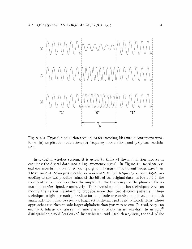
4.1. OVERVIEW: THE DIGITAL MODULATOR 41

"1" "0" "1"

Tb

(b)

(c)

(a)

Figure 4-2: Typical modulation techniques for encoding bits into a continuous wave-

form: (a) amplitude modulation, (b) frequency modulation, and (c) phase modula-

tion.

In a digital wireless system, it is useful to think of the modulation process as

encoding the digital data into a high frequency signal. In Figure 4-2 we show sev-

eral common techniques for encoding digital information into a continuous waveform.

These various techniques modify, or modulate, a high frequency carrier signal ac-

cording to the two possible values of the bits of the original data; in Figure 4-2, the

modi�cation is made to either the amplitude, the frequency, or the phase of the si-

nusoidal carrier signal, respectively. There are also modulation techniques that can

modify the carrier waveform to produce more than two distinct patterns. These

techniques might use multiple values for amplitude or combine modi�cations to both

amplitude and phase to create a larger set of distinct patterns to encode data. These

approaches can then encode larger alphabets than just zero or one. Instead, they can

encode B bits as a single symbol into a section of the carrier waveform by using 2B

distinguishable modi�cations of the carrier sinusoid. In such a system, the task of the

42 CHAPTER 4. FLEXIBLE PROCESSING IN A DIGITAL TRANSMITTER

receiver is to distinguish among the 2B di�erent possible forms of the signal in order

to determine which symbol was transmitted in each speci�c time interval.

Another point to note regarding Figure 4-2 is that, in each case, the encoding of

successive symbols is separated into disjoint time intervals. This is not true in general,

and there are very good reasons why the sections of the encoded carrier waveform

corresponding to continuous symbols often overlap signi�cantly. We examine the

implications of these overlapping segments more in the sections to come.

Many di�erent modulation techniques have been devised for encoding a sequence

of input data symbols into a waveform that can be transmitted through a wireless RF

channel. Phase shift keying (PSK), frequency shift keying (FSK) and quadrature am-

plitude modulation (QAM) are just few of the more common techniques. The wireless

environment can vary signi�cantly for di�erent systems, and modulation techniques

are designed to provide di�erent sets of trade-o�s between system performance and

resource consumption. Some modulation formats can be optimized for high data-

rate, power-constrained applications, while others might enable relatively simple and

inexpensive receivers [Lee and Messerschmitt, 1994, Proakis, 1995].

A exible technique that can support many di�erent modulation techniques is

clearly useful. If we desire a system that can provide e�cient operation in a wide

range of environments while supporting di�erent applications, it is evident that we

may need to change between di�erent modulation techniques as we encode data for

wireless transmission.

4.2 Conventional Digital Waveform Generation

In this section we present some conventional approaches to waveform generation for

communications signals. The �rst subsection presents a typical technique for encoding

digital information into waveforms using pulse-amplitude modulation (PAM), which

can be generalized to include a broad class of linear modulation techniques that

are useful in di�erent environments and applications. Following this, we review a

technique known as direct digital synthesis (DDS) that has been used to e�ciently

generate simple discrete waveforms, such as sinusoidal carrier waveforms.

Following this review, we show how to extend some of the key ideas of DDS to

the synthesis of more complicated waveforms, and we describe a new technique for

digital waveform synthesis that provides many of the advantages of DDS in a more

exible and e�cient digital modulator.

4.2. CONVENTIONAL DIGITAL WAVEFORM GENERATION 43

4.2.1 Conventional techniques for digital modulation

Digital modulation can be viewed as modifying a sinusoidal carrier waveform to en-

code a sequence of data symbols for transmission. We can also view modulation as

mapping individual data symbols to distinct continuous waveforms known as pulses.

A composite waveform is formed by combining multiple, time-shifted pulses, which

are sent sequentially through the channel as a single continuous waveform, as in Fig-

ure 4-2. Particular sets of pulses for encoding the symbols are chosen for their spectral

properties and to enhance the receiver's ability to distinguish among di�erent possible

waveforms as it recovers the original data.

One widely used technique for constructing a set of pulses is to use scaled versions

of a single prototype pulse. In pulse-amplitude modulation, the �nal transmitted

waveform is a sum of time-shifted pulses, each weighted by an appropriate scaling

value that corresponds to the bit it represents. Although the input data are typically

binary, it is often useful to use more than two pulses, as we noted before. We often

map blocks of bits into data symbols, each of which encodes multiple input data

bits. For example, we may map blocks of two bits each into a set of four symbol

values, A = fa1; a2; a3; a4g, which correspond to four di�erent scaling values, say

f�3;�1;+1;+3g. In a PAM system, this would result in a set of four pulses that

have similar shape, but di�erent amplitudes. In this particular example, the set of

scaling constants are real-valued: they lie on a one-dimensional line.

In some modulation schemes, the scaling constants do not lie on a line, but rather

form a two dimensional pattern. In general, then, scaling constants corresponding to

di�erent symbols in the alphabet can be complex-valued. It is helpful to visualize

the set using a plot of the di�erent values in a symbol constellation. Figure 4-3 shows

two di�erent constellations, each with 16 di�erent (complex) values. The 16 symbols

in each of these constellations represent di�erent sequences of four bits of the input

data. To create the corresponding waveform, we use consecutive symbols values to

modulate versions of a prototype pulse, p(t), that are uniformly shifted in time:

s(t) =1X

k=�1

akp(t� kTb) (4.1)

Here s(t) is the resulting continuous waveform as a function of time, t. The summing

index k indexes the elements in the sequence of symbols, ak, that encode the original

data bits. The constant Tb (another term for symbol is baud) is the time interval

between consecutive shifts of the pulse as it encodes the data symbols. The sum

in (4.1) is over multiple shifted and scaled pulses because the duration of the pulse

can, in general, exceed the shift interval. This situation often occurs in systems that

are designed to be e�cient in their use of RF spectrum; a pulse that has a compact

44 CHAPTER 4. FLEXIBLE PROCESSING IN A DIGITAL TRANSMITTER

���� ��

����

��

���� ��

����

��

���� ��

����

��

����

����

����

����

��������

��

�� ����

��

����

����

��

����

����

����

��

���� ��

����

��

Re

Im

(a) (b)

Im

Re

Figure 4-3: Two symbol constellations used to map blocks of four bits into complex

symbols for PAM, commonly known as (a) 16-QAM and (b) 16-PSK.

frequency-domain representation will tend to have a long time-domain representation.

It is helpful to note here that using a set of complex-valued symbols will result in

a complex-valued s(t). Of course, a wireless channel can only convey one-dimensional

signals: the voltage signal coupled to the antenna for transmission is a real-valued

function of time. The complex-valued signals are therefore converted to real-valued

signals during the translation to higher frequencies prior to transmission.

Because we are speci�cally interested in generating discrete sequences, we also

de�ne a discrete form of (4.1) in which sn is a sequence of uniformly spaced samples

of s(t): sn = s(nTs), where Ts is the time interval between samples:

sn =1X

k=�1

akp[n� kNs] (4.2)

The discrete pulse p[n] is a discrete version of the pulse p(t) and the time shift has

now become a simple shift in the time index by kNs, where Ns is the (integer) number

of samples in the output sequence occurring in each symbol interval, Tb = NsTs.

In (4.2) weighted and shifted pulses are combined by simple addition to form

the output sequence that will eventually be converted to an analog waveform and

transmitted through the channel. The limits on the summation in (4.2) indicate that

each output sample may, in theory, depend on an in�nite number of symbols. In

practice, though, pulse shapes are used that have a �nite duration and often simply

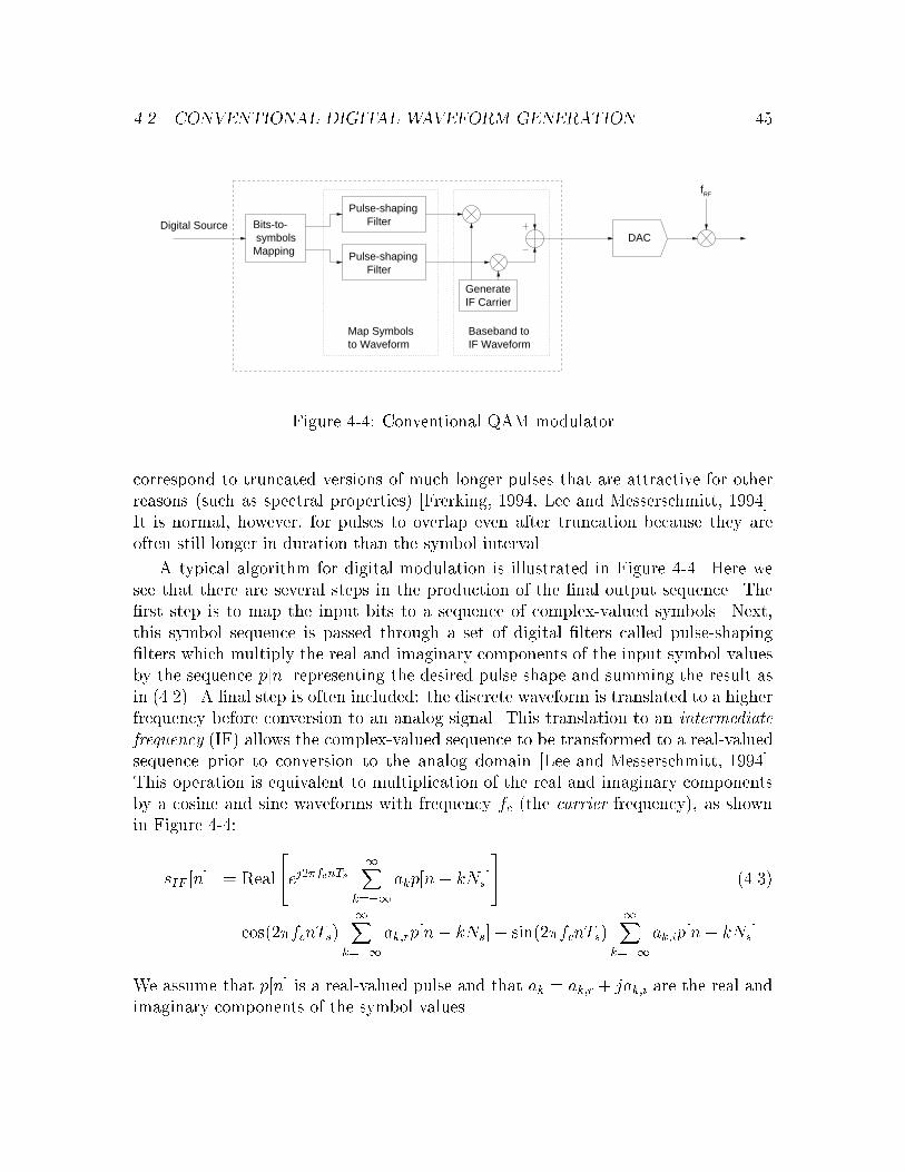
4.2. CONVENTIONAL DIGITAL WAVEFORM GENERATION 45

Bits-to- symbolsMapping

DAC

fRF

Pulse-shaping Filter

Pulse-shaping Filter

GenerateIF Carrier

Baseband toIF Waveform

Map Symbolsto Waveform

Digital Source

Figure 4-4: Conventional QAM modulator

correspond to truncated versions of much longer pulses that are attractive for other

reasons (such as spectral properties) [Frerking, 1994, Lee and Messerschmitt, 1994].

It is normal, however, for pulses to overlap even after truncation because they are

often still longer in duration than the symbol interval.

A typical algorithm for digital modulation is illustrated in Figure 4-4. Here we

see that there are several steps in the production of the �nal output sequence. The

�rst step is to map the input bits to a sequence of complex-valued symbols. Next,

this symbol sequence is passed through a set of digital �lters called pulse-shaping

�lters which multiply the real and imaginary components of the input symbol values

by the sequence p[n] representing the desired pulse shape and summing the result as

in (4.2). A �nal step is often included: the discrete waveform is translated to a higher

frequency before conversion to an analog signal. This translation to an intermediate

frequency (IF) allows the complex-valued sequence to be transformed to a real-valued

sequence prior to conversion to the analog domain [Lee and Messerschmitt, 1994].

This operation is equivalent to multiplication of the real and imaginary components

by a cosine and sine waveforms with frequency fc (the carrier frequency), as shown

in Figure 4-4:

sIF [n] = Real

24ej2�fcnTs 1X

k=�1

akp[n� kNs]

35 (4.3)

= cos(2�fcnTs)1X

k=�1

ak;rp[n� kNs]� sin(2�fcnTs)1X

k=�1

ak;ip[n� kNs]

We assume that p[n] is a real-valued pulse and that ak = ak;r + jak;i are the real and

imaginary components of the symbol values.

46 CHAPTER 4. FLEXIBLE PROCESSING IN A DIGITAL TRANSMITTER

So we see that the conventional approach is characterized by a series of mapping

steps: bit to symbols, symbols to discrete waveforms, and baseband waveforms to

IF waveforms. We will refer back to this series of mappings as we examine new

techniques to generate digital waveforms that provide both more exibility and more

computational e�ciency.

4.2.2 Direct digital synthesis of a sinusoidal carrier signal

To understand how we can develop new techniques to produce channel waveforms, it is

helpful to examine a waveform generation technique known as direct digital synthesis

(DDS), which has become increasingly popular in recent years.

This technique is well understood and widely used in the design of digital com-

munications systems. In this technique, a sinusoidal signal is synthesized from pre-

computed values instead of by computing the values of the samples as they are needed.

This technique can take several di�erent forms, depending on the amount of exibility

needed in the waveform to be synthesized.

Because a sinusoid is periodic, the single-frequency form of this technique e�-

ciently generates a sinusoid of �xed frequency: we simply pre-compute the samples

for a single period of the desired sinusoid and then cycle through and continuously

output these values to produce a continuous sinusoidal sequence. One requirement for

this technique is that we use an integral number of samples per cycle of the sinusoid.

In this case, Tc = kTs, the period of the carrier signal is a integral multiple of the

sample interval, Ts. This scheme provides no exibility as to the frequency of the

sinusoid generated, but it is computationally very e�cient.

A more powerful scheme, the phase-accumulator technique, uses a table of pre-

computed values and a phase accumulator to generate sinusoidal sequences of di�erent

frequencies. This approach uses a circular bu�er containing a large number of samples,

say 2N , of a single period of a sinusoid. A sinusoidal sequence with period of the form

Tc = 2NTs=k can be generated by outputting every kth sample in the circular bu�er.

The phase accumulator refers to an accumulator that stores the index value of the

current sample. This value corresponds to the phase value of the sinusoid that is

being generated.

This technique allows a system to avoid computing (and re-computing) in real-

time the values of the sinusoidal sequence, sn = cos(2�fcnTs), where fc is the desired

carrier frequency, by using the bu�er of pre-computed samples. These samples of a

transcendental function are particularly di�cult to generate in digital logic, and other

alternatives to this look-up table approach include approximation with Taylor series

or use of the cordic algorithm [Frerking, 1994].

The phase accumulator technique is more exible than the single-frequency tech-

nique because it can generate sinusoids with di�erent frequencies. This additional

4.3. DIRECT WAVEFORM SYNTHESIS FOR MODULATION 47

exibility, however, comes at the cost of reduced performance: we must compute

a new index value for each output sample. Although DDS techniques are relatively

straight forward, they can provide signi�cant computational savings in a digital trans-

mitter relative to a direct-computation approach. Relative to using a high-precision

analog oscillator, DDS has the advantage of using simple hardware components; it

can even be implemented in software.

4.3 Direct Waveform Synthesis for Modulation

In the previous section, we discussed two conventional techniques for generating dis-

crete waveforms for communications systems. We �rst discussed a typical imple-

mentation of a digital modulator, which computes each output sample using the

summation representation shown in (4.2). We also discussed DDS: a technique for

synthesizing relatively simple waveforms, such as sinusoids, using a look-up table of

pre-computed output samples. This technique required only a simple computation to

�nd the correct index in a table for each output sample to be produced.

In this section we apply some of the ideas from DDS to produce a new simple and

e�cient digital modulation technique. Our goal here is to produce a digital modulator

that can easily synthesize a discrete waveform using a table of pre-computed output

samples, thereby greatly reducing the computation required in a digital transmitter.

There are two challenges that must be overcome to produce a practical digital

modulation technique that uses less computation. First, the technique requires a

mapping from input bits to output samples that works in the general case of overlap-

ping transmit pulses. Equation (4.2) showed that each output sample might depend

on a large number of input bits; we will show that this condition does not preclude

look-up table technique similar to DDS, but that it can lead to prohibitively large

look-up tables in some situations.

This is the second challenge: many DDS implementations use table with tens to

hundreds of entries, and many tricks have been developed to reduce even these modest

tables to smaller sizes [Frerking, 1994, Reed, 1998]. The most straight forward look-

up tables for a digital modulator can contain thousands or millions of entries. Such

a modulator may not be feasible, even though 256 megabits of memory may soon be

available on a single chip.

We overcome this second challenge by decomposing a large look-up table into

smaller tables, whose total size is also much smaller than the single original. Di�erent

decompositions provide a wide range of operating points that enable a exible trade-

o� between computation and memory requirements.

In the next sections, we describe the direct waveform synthesis (DWS) technique

for directly synthesizing a baseband digital waveform. We also extend the basic DWS

48 CHAPTER 4. FLEXIBLE PROCESSING IN A DIGITAL TRANSMITTER

-4T -3T -2T -T 0 T 2T 3T 4T

Figure 4-5: Typical sin(x)=x pulse shape for a bandwidth-e�cient system, where

x = �t=T and T is the symbol interval.

technique to allow the synthesis of digital waveforms at passband, thereby removing

the need to translate the baseband waveform to IF, and also to allow the mapping

of multiple symbols at a time, thereby providing more exibility in the computation-

memory trade-o�.

4.3.1 A new approach to modulation: Direct mapping

It is useful here to look at a typical pulse shape used in digital communications

systems. Figure 4-5 shows such a pulse, which has the characteristic sin(x)=x shape

that is typical of pulses used in systems where it is important to use the available

RF spectrum e�ciently. Pulses with this shape maximize the rate at which data

symbols can be transmitted minimizing the width of the frequency band used for the

transmission. We discuss further properties of these pulses in Chapter 6, where we

discuss reception.

A true sin(x)=x pulse shape has an in�nite duration in time, so modulators approx-

imate it by symmetrically truncating the pulse to K symbol periods. This truncation

tends to spread the energy of the pulse into adjacent frequency bands, and the degree

of truncation must be chosen to balance this spreading with the computational sav-

ings of truncation. The choice of the speci�c value of K used to approximate a longer

pulse is not the focus of this work, but speci�c e�ects of truncation are described

4.3. DIRECT WAVEFORM SYNTHESIS FOR MODULATION 49

Address Table

Compute Index

Look-upDigital Source

DAC

fRF

waveform at IFN samples ofs

Figure 4-6: Proposed QAM modulator

in [Welborn, 1999]. In this work our results will be derived in terms of an arbitrary

K.

In any case, the pulses used to transmit consecutive symbols will overlap in time

because truncation to a single symbol period spreads too much energy. From (4.2)

we see that we need sum only over the symbols for which the shifted version of p[n]

is non-zero:

sn =X

k: p[n�kNs]6=0

akp[n� kNs] (4.4)

From this result we begin to see how we can pre-compute the output samples

sn. Each output sample depends on K input symbols, or BK bits when we use a

constellation of 2B symbols. During a single symbol interval, Ns output samples all

depend on the same K input symbols, that is, the output waveform in that interval

is completely determined by K input symbols.

To produce our direct mapping, it is now clear that we can map a sequence of BK

input bits to Ns output samples. In this way, we can produce a look-up table that

contains all possible symbol-length sequences of output samples by computing these

sequences for all possible 2BK sequences of input bits. Once we have produced this

table, we can use it to e�ciently synthesize a continuous sequence that corresponds

to the discrete-time digital waveform. This technique is shown in Figure 4-6. The

steps of this direct waveform synthesis technique in its simplest form are summarized

here:

50 CHAPTER 4. FLEXIBLE PROCESSING IN A DIGITAL TRANSMITTER

-3

-2

-1

0

1

2

3

-4T -3T -2T -T 0 T 2T 3T 4T

-3

-2

-1

0

1

2

3

-4T -3T -2T -T 0 T 2T 3T 4T

-3

-2

-1

0

1

2

3

-4T -3T -2T -T 0 T 2T 3T 4T

-3

-2

-1

0

1

2

3

-4T -3T -2T -T 0 T 2T 3T 4T

-3

-2

-1

0

1

2

3

-4T -3T -2T -T 0 T 2T 3T 4T

-3

-2

-1

0

1

2

3

-4T -3T -2T -T 0 T 2T 3T 4T

-3

-2

-1

0

1

2

3

-4T -3T -2T -T 0 T 2T 3T 4T

-3

-2

-1

0

1

2

3

-4T -3T -2T -T 0 T 2T 3T 4T

-3

-2

-1

0

1

2

3

-4T -3T -2T -T 0 T 2T 3T 4T

-3

-2

-1

0

1

2

3

-4T -3T -2T -T 0 T 2T 3T 4T

-3

-2

-1

0

1

2

3

-4T -3T -2T -T 0 T 2T 3T 4T

Figure 4-7: Section of a synthesized 4-PAM waveform with Ns = 8 samples per

symbol interval. Individual table entries are indicated by boxes.

Step 0: Compute entries of look-up table for all 2BK possible input bit

sequences. Prepend bit sequence to be transmitted with B(K�1)dummy bits to initialize modulator. Set k = 0.

Step 1: Compute index for table entry using bitsBk+1 throughB(k+K).

Output Ns samples of the discrete output waveform, sn.

Step 2: Set k = k + 1, goto Step 1.

Figure 4-7 shows a typical section of a synthesized waveform where each table entry

(indicated by boxes) contains eight samples of a discrete waveform. It is important

to note that this algorithm does not produce an approximation to the waveform pro-

duced using the conventional technique shown in Figure 4-4. Both schemes produce

exactly the same output sequence when they use the same pulse shape and associ-

ated parameters. Even the conventional technique must use an approximation to any

in�nite-length pulse in order to implement the digital pulse shaping �lter. Although

they are separate table entries, the segments of output samples produced using the

DWS technique will always \�t together" to form a smooth, continuous sequence

because of the process of using a sliding window of BK input bits.

4.3. DIRECT WAVEFORM SYNTHESIS FOR MODULATION 51

4.3.2 Decomposing tables to reduce memory

The size of the look-up table is 2BK � Ns � W bytes when an output sample is

W byte. For example, a 4-PAM system (B = 2) with a 6 symbol-length pulse-

shaping transmit �lter (K = 6) generating 10 samples per symbol (Ns = 10) and 2

bytes/sample requires a table size of 80 Kbytes, which is quite reasonable and would

actually �t in the cache on most modern processors. For larger constellations or longer

pulses the table size grows rapidly (exponentially in the length of the pulse or number

of bits/symbol). For example, a 16-QAM system (B = 4) using an 8 symbol-length

pulse-shaping transmit �lter generating 10 samples per symbol and 2 bytes/sample

would require 80 gigabytes to store the look-up table.

One way to reduce this growth in table size is to decompose the large table into

several smaller tables in which we perform multiple look-ups of partial waveforms and

then add the pre-computed values to produce the �nal waveform. To use this tech-

nique we must �nd an appropriate way to decompose the required sample sequences.

This decomposition must satisfy two requirements. First, it must be \linear" in the

sense that we can sum values obtained from decomposed tables to produce the same

�nal output value as would be produced by the original table. Second, each compo-

nent table must depend on a smaller number of input bits so that total size of the

smaller tables is less than the size of the original table.

One solution that satis�es both requirements is to decompose the original table

intoD separate tables by having the index of each table depend only on K

Dconsecutive

symbols (or BK

Dconsecutive bits) instead of the fullK symbols (or BK bits), as shown

in Figure 4-8. It other words, each table contains partial sums of only K=D terms

from (4.4) instead of full sums of K terms, as in the original table. In the extreme

case of D = K, each table has 2B entries that correspond to scaled versions of the

pulse p[n] for each symbol in the constellation.

Now the total table space using the decomposition is D � 2BK

D � Ns �W bytes,

and the cost of using this decomposition is that we perform D look-ups in each

symbol interval and D � 1 additions for every output sample produced. (The actual

cost is less: we can use the same index computation result in each of the D tables

in consecutive steps. This way we still only perform one index computation per

symbol.) The previous example of a 16-QAM system with an 8 symbol-length pulse-

shaping �lter would now require 4 � 28 � Ns � W = 20 kilobytes (with D = 4)

or 2 � 216 � Ns � W � 2:5 megabytes (with D = 2) when Ns = 10 and W = 2

bytes/sample.

52 CHAPTER 4. FLEXIBLE PROCESSING IN A DIGITAL TRANSMITTER

Delay

Delay

Delay

Delay

��������������������

��������

DigitalSource

Waveform Samples

Lookup Table

Lookup Table

Input: B x K / D bitsOutput: N x W bytess

Figure 4-8: QAM modulator using parallel look-ups to reduce table size.

4.3.3 Extensions of direct waveform synthesis

Direct synthesis of passband waveforms

In our discussion of the conventional approaches to digital modulation, we noted that

a digital modulator often produces the baseband digital waveform and then translates

it to a higher frequency prior to conversion to the analog domain.

This DWS technique can be modi�ed to directly produce a digital waveform that

has already been translated to IF. This approach is useful when we need to produce

an output waveform that contains multiple signals combined using frequency mul-

tiplexing, as might be done in a wideband cellular or PCS transmitter. For such a

system, each of the individual signals can be generated at passband with the correct

center frequency and then simply added to produce the desired composite waveform.

We can see how DWS can be used to produce a digital waveform at passband by

rewriting (4.4) from above:

sIF [n] = Real

24ej2�fcnTs 1X

k=�1

akp[n� kNs]

35

4.3. DIRECT WAVEFORM SYNTHESIS FOR MODULATION 53

=X

k: p[n�kNs]6=0

mk cos(2�fcnTs + �k)p[n� kNs] (4.5)

where ak = mkej�k is the magnitude-phase form of the complex symbol value. We

will assume that the pulse shape p[n] is real-valued in (4.5), although we can still

use this technique for a complex-valued p[n] if we modify the equations properly.

In order to synthesize the digital waveform at passband as above, we combine the

cosine term and the pulse sequence p[n] in (4.5). If we restrict ourselves to using an

IF carrier frequency that has an integral number of periods in one symbol interval,

fc = m=(NsTs) for some integer m, then we can combine the frequency translation

into the pulse shape by de�ning pIF (t) = cos(2�fct)p(t). The time-shifted versions of

the discrete form of this pulse now become:

pIF [n� kNs] = [cos(2�fct)p(t)]t=nTs�kNsTs = cos(2�fcnTs � 2km�)p[n� kNs] (4.6)

This shows that the composite pulse pIF [n] can be shifted in time by any number of

symbol periods without a�ecting the frequency translating component because of the

2�-periodicity of the cosine term. We can now rewrite the equation for the passband

signal using the composite pulse:

sIF [n] =X

k: p[n�kNs] 6=0

mk cos(2�fcnTs + �k)p[n� kNs] =X

k: p[n�kNs]6=0

mkpIF;k[n� kNs]

(4.7)

To synthesize a waveform at passband, we simply use the same technique as before,

but we compute the entries in the look-up table using the composite pulse sequence

pIF;k[n] = cos(2�fcnTs + �k)p[n].

Storing multiple symbols per table entry

In an earlier section we discussed how the DWS technique can result in an extremely

large table in some situations and how this table growth can be alleviated through

table decomposition. The technique allowed us to select from several di�erent de-

compositions (i.e., D = 1; 2; :::) for a waveform in order to trade-o� between memory

requirements and computational complexity. It is also possible to generalize the DWS

technique to produce sample sequences for multiple symbols with each table look-up.

Instead of mapping K input symbols to a segment of output samples representing a

single symbol interval, we could map (K +M � 1) input symbols to an M -symbol

interval. This technique could allow us to only marginally increase the number of

input symbols (especially if K is relatively large) and yet produce two or three times

as many output samples with each look-up. The point of this generalization is not

to replace the special case of M = 1, but simply to provide the system designer with

54 CHAPTER 4. FLEXIBLE PROCESSING IN A DIGITAL TRANSMITTER

more options to trade-o� between memory and computation in a digital waveform

synthesizer.

Using this generalization, each table entry now containsM�Ns samples and there

are 2B�(K+M�1) entries if we use a single table. The total memory space required for

the general case using a decomposition is now: D� 2B�(K+M�1)

D �M �Ns�W bytes

and the cost of using the table decomposition to reduce memory is still the same: we

perform D � 1 additions for each output sample.

One case in which this technique of storing multiple symbol intervals in each table

entry is useful is in �=4-di�erential-quadrature PSK (�=4-DQPSK), which is used in

digital cellular radio systems [Wiesler and Jondral, 1998]. In this modulation format,

two di�erent sets of four symbols (with a 45o rotational o�set) are used to alternately

encode the data. In this situation, the modulator needs to maintain some state to

determine which constellation should be used for encoding, and to use two tables for

the di�erent cases. If the DWS technique is used to produce the waveform, blocks

of four bits could be mapped directly to segments that are two symbol-periods in

length, and there would be no need to maintain any state or multiple tables.

4.4 Performance and Resource Trade-o�s

4.4.1 Performance comparison

To compare our proposed architecture with the conventional architecture, we have

tabulated the operation counts required to produce a single output sample for each

scheme.

The operations required to produce a single output sample of a digital waveform

at IF using the conventional architecture (as in Figure 4-4) are summarized in Table

4.1. In this table we assume that the local oscillator that generates the IF carrier

is implemented using direct digital synthesis techniques. For the proposed DWS

architecture, Table 4.2 summarizes the operations required to produce a single output

sample. In this case, the operations required to compute the table index are performed

only once for each sequence of MNs samples, which are stored in a contiguous region

of the look-up table.

An example of the total operations required for a typical modulator is helpful to

understand the di�erence in operations required for these two approaches. For the

case of a 1 M-baud (1 million symbols/second) modulator with Ns = 8 and K = 4,

the total operation count is summarized for each function below.

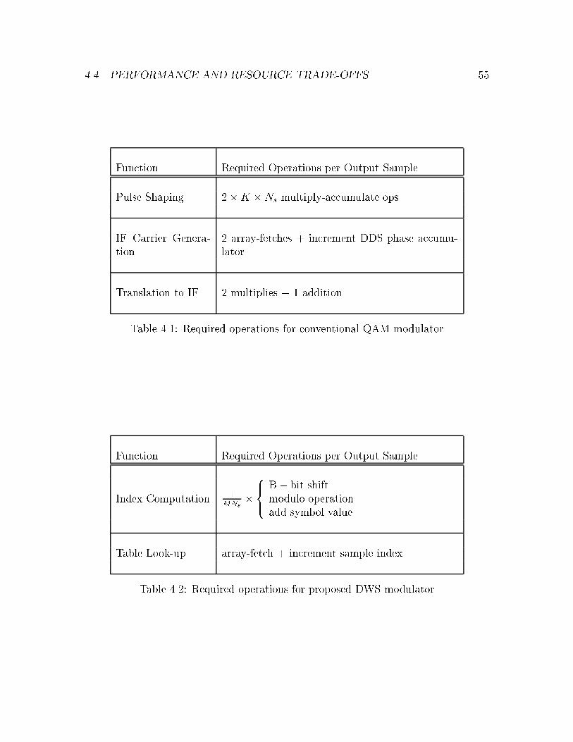
4.4. PERFORMANCE AND RESOURCE TRADE-OFFS 55

Function Required Operations per Output Sample

Pulse Shaping 2�K �Ns multiply-accumulate ops

IF Carrier Genera-

tion

2 array-fetches + increment DDS phase accumu-

lator

Translation to IF 2 multiplies + 1 addition

Table 4.1: Required operations for conventional QAM modulator

Function Required Operations per Output Sample

Index Computation 1MNs

�

8><>:

B� bit shift

modulo operation

add symbol value

Table Look-up array-fetch + increment sample index

Table 4.2: Required operations for proposed DWS modulator

56 CHAPTER 4. FLEXIBLE PROCESSING IN A DIGITAL TRANSMITTER

Conventional approach:

� Pulse Shaping: 2 � 4 � 8 MACs � 8 million samples/second= 512 millions

MACs/second

� IF Carrier Generation: 16 million array-fetches/second + 8 million increments

per second

� Translate to IF: 16 million multiplies/second + 8 million adds/second

Direct waveform synthesis approach:

� Index computation: 1 million �( bit-shift + power-of-two modulo operation +

addition) per second

� Table Look-up: 8 million array-fetches/second + 8 million increments/second

Clearly the DWS technique required much fewer operations. Although there are

several di�erent types of operations involved, there is about a factor of 25 di�erence

between the total counts for the two: about 20 million operations per second compared

to 500+ million operations per second for the conventional approach. Even this

higher number seems modest by today's standards, but when we consider scaling to

a system that modulates billions of symbols per second, the di�erences become more

substantial.

4.4.2 Memory versus computation

The trade-o�s provided between use of memory and computation through the use of

DWS are fairly straightforward. In the most general case, the total amount of memory

required isD�2B�(K+M�1)

D �M�Ns�W bytes and the computation is essentiallyD�1addition operations per output sample. Because of the many parameters in the above

equation, we have included a few plots that illustrate the di�erent trade-o�s available

for a typical set of parameters. In Figure 4-9 we show the total memory requirements

for both a 8-PAM system and a 16-QAM system. These plots show the trade-o�

between memory usage and computation using the table decomposition described

above to generate sample sequences for multiple (M) symbols. The computation

required in each case shown in the plots is determined by the value of D used to

decompose the table (the computation is D�1 additions per output sample). In each

of these two plots, the most important point is that there are a variety of operating

points (indicated by the points where D divides K + M � 1 on the various lines),

allowing the system to choose between the use of memory and computation according

to other constraints that might exist in the system.

4.4. PERFORMANCE AND RESOURCE TRADE-OFFS 57

100

1000

10000

100000

1e+06

1e+07

1e+08

1 2 3 4 5 6 7 8 9 10 11

Tot

al ta

ble

size

(by

tes)

Length of output sequence in look-up table (in M = number of symbol intervals)

(a) 8-PAM with B=2, K=6, Ns = 10, W=2

D=1D=2

D=3

D=4

D=8

100

1000

10000

100000

1e+06

1e+07

1e+08

1 2 3 4 5 6 7 8 9 10 11

Tot

al ta

ble

size

(by

tes)

Length of output sequence in look-up table (in M = number of symbol intervals)

(a) 8-PAM with B=2, K=6, Ns = 10, W=2

D=1D=2

D=3

D=4

D=8

100

1000

10000

100000

1e+06

1e+07

1e+08

1 2 3 4 5 6 7 8 9 10 11

Tot

al ta

ble

size

(by

tes)

Length of output sequence in look-up table (in M = number of symbol intervals)

(a) 8-PAM with B=2, K=6, Ns = 10, W=2

D=1D=2

D=3

D=4

D=8

100

1000

10000

100000

1e+06

1e+07

1e+08

1 2 3 4 5 6 7 8 9 10 11

Tot

al ta

ble

size

(by

tes)

Length of output sequence in look-up table (in M = number of symbol intervals)

(a) 8-PAM with B=2, K=6, Ns = 10, W=2

D=1D=2

D=3

D=4

D=8

100

1000

10000

100000

1e+06

1e+07

1e+08

1 2 3 4 5 6 7 8 9 10 11

Tot

al ta

ble

size

(by

tes)

Length of output sequence in look-up table (in M = number of symbol intervals)

(a) 8-PAM with B=2, K=6, Ns = 10, W=2

D=1D=2

D=3

D=4

D=8

100

1000

10000

100000

1e+06

1e+07

1e+08

1 2 3 4 5 6 7 8 9 10 11

Tot

al ta

ble

size

(by

tes)

Length of output sequence in look-up table (in M = number of symbol intervals)

(a) 8-PAM with B=2, K=6, Ns = 10, W=2

D=1D=2

D=3

D=4

D=8

100

1000

10000

100000

1e+06

1e+07

1e+08

1 2 3 4 5 6 7 8 9 10 11

Tot

al ta

ble

size

(by

tes)

Length of output sequence in look-up table (in M = number of symbol intervals)

(a) 8-PAM with B=2, K=6, Ns = 10, W=2

D=1D=2

D=3

D=4

D=8

100

1000

10000

100000

1e+06

1e+07

1e+08

1 2 3 4 5 6 7 8 9 10 11

Tot

al ta

ble

size

(by

tes)

Length of output sequence in look-up table (in M = number of symbol intervals)

(a) 8-PAM with B=2, K=6, Ns = 10, W=2

D=1D=2

D=3

D=4

D=8

100

1000

10000

100000

1e+06

1e+07

1e+08

1 2 3 4 5 6 7 8 9 10 11

Tot

al ta

ble

size

(by

tes)

Length of output sequence in look-up table (in M = number of symbol intervals)

(a) 8-PAM with B=2, K=6, Ns = 10, W=2

D=1D=2

D=3

D=4

D=8

100

1000

10000

100000

1e+06

1e+07

1e+08

1 2 3 4 5 6 7 8 9 10 11

Tot

al ta

ble

size

(by

tes)

Length of output sequence in look-up table (in M = number of symbol intervals)

(a) 8-PAM with B=2, K=6, Ns = 10, W=2

D=1D=2

D=3

D=4

D=8

100

1000

10000

100000

1e+06

1e+07

1e+08

1 2 3 4 5 6 7 8 9 10 11

Tot

al ta

ble

size

(by

tes)

Length of output sequence in look-up table (in M = number of symbol intervals)

(b) 16-QAM with B=4, K=6, Ns = 10, W=2

D=2 D=3 D=4

D=8

100

1000

10000

100000

1e+06

1e+07

1e+08

1 2 3 4 5 6 7 8 9 10 11

Tot

al ta

ble

size

(by

tes)

Length of output sequence in look-up table (in M = number of symbol intervals)

(b) 16-QAM with B=4, K=6, Ns = 10, W=2

D=2 D=3 D=4

D=8

100

1000

10000

100000

1e+06

1e+07

1e+08

1 2 3 4 5 6 7 8 9 10 11

Tot

al ta

ble

size

(by

tes)

Length of output sequence in look-up table (in M = number of symbol intervals)

(b) 16-QAM with B=4, K=6, Ns = 10, W=2

D=2 D=3 D=4

D=8

100

1000

10000

100000

1e+06

1e+07

1e+08

1 2 3 4 5 6 7 8 9 10 11

Tot

al ta

ble

size

(by

tes)

Length of output sequence in look-up table (in M = number of symbol intervals)

(b) 16-QAM with B=4, K=6, Ns = 10, W=2

D=2 D=3 D=4

D=8

100

1000

10000

100000

1e+06

1e+07

1e+08

1 2 3 4 5 6 7 8 9 10 11

Tot

al ta

ble

size

(by

tes)

Length of output sequence in look-up table (in M = number of symbol intervals)

(b) 16-QAM with B=4, K=6, Ns = 10, W=2

D=2 D=3 D=4

D=8

100

1000

10000

100000

1e+06

1e+07

1e+08

1 2 3 4 5 6 7 8 9 10 11

Tot

al ta

ble

size

(by

tes)

Length of output sequence in look-up table (in M = number of symbol intervals)

(b) 16-QAM with B=4, K=6, Ns = 10, W=2

D=2 D=3 D=4

D=8

100

1000

10000

100000

1e+06

1e+07

1e+08

1 2 3 4 5 6 7 8 9 10 11

Tot

al ta

ble

size

(by

tes)

Length of output sequence in look-up table (in M = number of symbol intervals)

(b) 16-QAM with B=4, K=6, Ns = 10, W=2

D=2 D=3 D=4

D=8

100

1000

10000

100000

1e+06

1e+07

1e+08

1 2 3 4 5 6 7 8 9 10 11

Tot

al ta

ble

size

(by

tes)

Length of output sequence in look-up table (in M = number of symbol intervals)

(b) 16-QAM with B=4, K=6, Ns = 10, W=2

D=2 D=3 D=4

D=8

Figure 4-9: Plots showing memory requirements versus number of symbol periods per

table entry for (a) 8-PAM and (b) 16-QAM waveform synthesis with K = 6, Ns = 10.

58 CHAPTER 4. FLEXIBLE PROCESSING IN A DIGITAL TRANSMITTER

Modulation Algorithm Transmit Rate

BPSK (K=16) Table Look-up 18.9 Mbit/sec

(512 Kbytes, D=1)

Direct Computation 0.3 Mbit/sec

16-QAM (K=16) Table Look-up 28.3 Mbit/sec

(2048 Kbytes, D=4)

Direct Computation 1.2 Mbit/sec

16-QAM (K=10) Table Look-up 36.8 Mbit/sec

(16384 Kbytes, D=2)

Direct Computation 1.9 Mbit/sec

16-QAM (K=4) Table Look-up 72.2 Mbit/sec

(512 Kbytes, D=1)

Direct Computation 4.6 Mbit/sec

64-QAM (K=8) Table Look-up 38.7 Mbit/sec

(128 Kbytes, D=4)

Direct Computation 3.6 Mbit/sec

Table 4.3: Results of software implementations of conventional QAM modulator and

DWS modulator.

4.5 Empirical Performance Evaluation

To provide a further comparison of the DWS technique, we have implemented both

DWS and a conventional modulator (represented by Figure 4-4 and Table 4.1) in

software. To determine the relative performance of each, we measured the time

required for each technique to modulate a large number of data symbols. The results

of this test are presented as maximum transmission rates indicated by measure run-

times and are summarized in Table 4.5 for a number of di�erent cases. These di�erent

cases include three constellation sizes and di�erent lengths for the pulse-shaping �lter.

For the DWS implementation, the table also shows the amount of memory that was

required for the look-up table. The tests were performed using a laptop with a 366

kHz Celeron processor with a 256 kByte cache.

In most cases, DWS was able to support a transmission about 20� higher than

the conventional approach. This improvement is even seen when the required look-

up table was far too large to �t in the cache of the processor. In the last case

shown, 64-QAM, only a 10� performance improvement was indicated. In this case,

the relatively poor performance of DWS is probably due to the decomposition into

four smaller tables to obtain a reasonable total memory size (using D=2 would have

4.6. IMPLEMENTATION OF A DWS MODULATOR 59

required 256 Mbytes of memory).

4.6 Implementation of a DWS Modulator

An implementation of the DWS modulation algorithm was done as part of the Spec-

trumWare Project at the MIT Laboratory for Computer Science. In this project,

we have developed hardware and software components that enable the implemen-

tation of wireless communications systems in which all of the physical layer pro-

cessing is performed in software on a general purpose computer. Details of both

the RF interface hardware and the software programming environment are available

in [Bose et al., 1999, Ismert, 1998, Bose, 1999].

The DWS algorithm was implemented in this software radio environment to study

the usefulness of a exible wireless transmitter architecture. Figure 4.6 shows the

graphical user interface for the DWS modulator, a time-domain trace of the synthe-

sized digital waveform, and a constellation diagram detected by looping the digital

signal back to the receive portion of the system. The user interface provides software

control of a number of feature of the system, including modulation format, receiver

�lter size and symbol timing and phase recovery controls.

This DWS implementation was used in an investigation of an adaptive voice com-

pression and modulation scheme presented in [Rao, 2000]. This work demonstrates

a system that uses a number of di�erent voice compression algorithms and the ex-

ible DWS modulator to provide e�cient voice communications under a wide range

of di�erent SNR conditions. Under favorable conditions, the system provides higher

quality voice using a high data rate compression and large constellation. Under

worsening SNR conditions, better voice quality is attained by switching to voice com-

pression algorithms that require lower bit-rates and using successively smaller signal

constellations to improve the bit-error rate.

An example of this concept is illustrated in Figure 4.6. Here we see an 8-PSK

constellation under two di�erent levels of SNR. At the lower level, excessive bit-error

rate can be prevented by switching to a 4-PSK constellation that provides a lower

bit-rate with a lower BER.

4.7 Summary

Direct waveform synthesis provides a signi�cant performance improvement over con-

ventional approaches to digital modulation. This gain comes from its ability to di-

rectly synthesize waveforms using a simple table look-up based on the input bits to

the modulator. We have also presented a technique that provides a exible trade-o�

60 CHAPTER 4. FLEXIBLE PROCESSING IN A DIGITAL TRANSMITTER

Figure 4-10: Graphical user interface for an implementation of a direct waveform

synthesis digital modulator.

4.7. SUMMARY 61

(a)

(b)

(c)

Figure 4-11: Received signal constellation diagrams for (a) 8-PSK under relatively

high SNR (b) 8-PSK under low SNR and (c) 4-PSK under low SNR.

62 CHAPTER 4. FLEXIBLE PROCESSING IN A DIGITAL TRANSMITTER

between computation and memory usage for DWS by allowing the mapping to be

implemented using a number of smaller tables instead of a single large table.

In the context of a wireless communications system, the digital modulator does

not need to provide much exibility during operation. Any change to the modulation

format will require coordination between receiver and transmitter, and such changes

will therefore tend to be infrequent. DWS provides a good balance of e�cient perfor-

mance, exible implementation properties and the ability to be recon�gured if channel

conditions or system requirements so dictate.

Chapter 5

Flexible Processing in a Digital

Receiver

We have characterized the channel coder function in a wireless transmitter as a one-

to-one mapping from a sequence of data bits into a sequence of distinctive pulses for

transmission. At the receiver, the primary task is to reverse this mapping, thereby

recovering the original data bit-stream. After this channel decoding, source decoding

reproduces the original source information.

In Figure 5-1 we see a representation of the processing steps performed in the

receiver. Also shown in this �gure is a further decomposition of the channel decoder

into several speci�c functions. The �rst two of these functions are channel separation

and symbol detection. The combined task of these two functions is to reproduce

the error-encoded bit stream passed to the digital modulator in the transmitter. Of

course, the sequence of bits produced at the output of the detector may contain

errors. Because the original encoded sequence contained some controlled amount

of redundancy, the error decoder can detect the presence of many errors and either

correct them or take other appropriate actions to handle the corrupted data.

In this work, we examine the processing required for the functions of channel

ChannelSeparation Decoder

Error

WirelessChannel

SymbolDetection

SourceDecoder

User

Channel Decoder

Figure 5-1: Required processing steps in a digital receiver.

63

64 CHAPTER 5. FLEXIBLE PROCESSING IN A DIGITAL RECEIVER

separation and symbol detection. Our �rst goal is to develop a more fundamental

understanding of the functionality required by these two processing steps in the digital

domain. We then use this understanding to develop algorithms that provide both

exibility and improved e�ciency over conventional techniques in a wide range of

situations.

The channel decoder is traditionally divided into the speci�c steps of channel

separation and detection because the wireless channel is a shared medium that com-

bines many signals. The distortion caused by the channel takes on several forms:

additive interfering signals, random noise, delayed versions of the same signal, etc.

We therefore model the input to a digital receiver as a sum of an indexed sequence,

sn, representing the signal of interest, with I interfering signals from other nearby

transmitters and a random noise component, nn:

rn = sn +IXi=1

si;n + nn (5.1)

The overall process of channel decoding requires the recovery of the transmitted

data from this received signal. Algorithms for this type of analysis are sensitive

to interference in the input signal, but often perform well in the presence of only

additive random noise. We therefore divide the processing of the received wideband

signal into two stages: �rst, the channel separation stage removes interfering signals,

transforming the input sequence into another sequence that is simply a noisy version

of the original signal, from which the detector produces an estimate of the original

data encoded by the digital modulator.

In the next few sections we discuss the problems of channel separation in more

detail and describe current techniques used to solve these problems. We then present

several new techniques that enable us to perform the functions required in a chan-

nel separator in manner that provides both exibility and greater e�ciency than

conventional approaches. We discuss the problem of detection, the second stage of

processing, in the next chapter.

5.1 Overview: Channel Separation

We have seen that the discrete sequence of samples at the input to a wideband receiver

is the sum of the desired signal and undesired interfering signals. We also assume that

the signal contains additive random noise. This noise includes several e�ects, such

as low level random signals picked up by the antenna and thermal noise generated

inside the analog circuitry of the receiver.

The goal of channel separation is to prepare the received sequence, enabling the

5.1. OVERVIEW: CHANNEL SEPARATION 65

detector to recover the original data sequence from the received signal. Stated another

way, the channel separator should produce a sequence containing components in the

received signal corresponding to the signal of interest, while removing the interference.

To facilitate separation, it is common to restrict, through regulation, the emis-

sions of potential interfering transmitters, so that any interfering signals will occur

in disjoint frequency bands in the RF spectrum. This technique for providing multi-

ple access to the physical medium is known as frequency division multiple access or

FDMA. Other techniques such as time division multiple access (TDMA) and code

division multiple access (CDMA) can also be used to allow multiple transmitters to

share the same band of frequencies, but are not addressed here. In FDMA, sepa-

rating the desired signal from potential adjacent channel interferers is equivalent to

extracting from the received sequence only those components that occur within the

band of frequencies corresponding to the signal of interest.

This separation is accomplished through the use of digital �lters that pass sig-

nal components in the desired band of frequencies, the passband, and attenuate sig-

nal components outside of this band, in the region known as the stopband. In a

wideband receiver the use of digital �lters to perform channel separation can lead

to an implementation with very high computational complexity. For a receiver

in which the channel separation is performed in the digital domain, the work re-

quired to extract individual channels from the input of a wideband receiver pro-

vides a �rst-order estimate of the computational resources required for the entire

receiver [Mitola, 1995, Wepman, 1995].

The reasons for this high computational burden are several. First, a wideband dig-

ital receiver will necessarily have a high input sample rate to adequately represent the

wideband input signal. In addition, to cleanly extract a narrow band of frequencies,

the receiver must accurately resolve those frequencies at the boundary of the band of

interest. These two conditions combine to produce a situation that can require large

amounts of processing to perform channel separation using conventional techniques.

Before addressing this problem, however, we examine the basic steps that are widely

used to perform the entire channel separation procedure using digital �lters.

In Figure 5-2 we see the conceptual steps that are often used to perform channel

separation. The results of these same steps on a hypothetical wideband signal (repre-

sented in the frequency domain) are shown in Figure 5-3. First, there is a frequency

translation step. Here the wideband signal is shifted in frequency to bring the band of

interest into the passband of a digital �lter and the interfering signals into the stop-

band. This translation is represented in Figure 5-2 by a multiplication of the received

sequence and a complex sinusoidal sequence. The magnitude of the frequency shift

is determined by the frequency of the complex sinusoidal sequence.

The second step in this process is bandwidth reduction. Here the �lter produces

66 CHAPTER 5. FLEXIBLE PROCESSING IN A DIGITAL RECEIVER

D

FrequencyTranslation

Narrowband Output

Sample Rate Reduction

Wideband Input

BandwidthReduction

Complex Sinusoid

Filter

Figure 5-2: Typical processing for narrowband channel selection.

an output sequence in which the components at di�erent frequencies are attenuated

or ampli�ed according to the frequency response of the �lter. Because this output

sequence does not contain any signi�cant components outside the band of interest,

it is now possible to represent the desired signal using a lower sample rate with-

out signi�cantly distorting those components within the band of interest. If there

were signi�cant signal components present outside the band of interest, reducing

the sample rate would cause aliasing of those components into the band of inter-

est [Oppenheim and Schafer, 1989]. Hence a �nal step of sample-rate reduction, or

decimation, reduces the rate of samples in the sequence by a constant factor D, the

decimation rate. This rate reduction is also important because it reduces the pro-

cessing load in subsequent stages.

Much of the work in this chapter was initially motivated by the desire to develop

e�cient techniques to perform the steps of the channel separation process in a wide-

band digital receiver implemented in software as part of the SpectrumWare project.

One of the early goals of this project was to implement such a receiver that could

extract a 30 kHz channel from a 25 mega-sample per second input sample stream. It

soon became clear that conventional approaches to frequency translation and �ltering

would result in a design that would require too much computation to run in real-time

on the 200 Mhz personal computers used in the implementation. Many of the results

presented in the remainder of this chapter have helped produce an e�cient software

implementation of a wideband receiver, which will be described in more detail in a

later section. In the next section, however, we �rst examine the speci�c steps of the

channel separation process in more detail and then review some of the techniques

that have been developed to perform them.

5.1. OVERVIEW: CHANNEL SEPARATION 67

Frequency0

Frequency0

Frequency0

Frequency/D0

Figure 5-3: Conceptual steps used for conventional approach to narrowband channel

selection: (a) frequency translation, (b) bandwidth reduction, and (c) sample rate

reduction.

68 CHAPTER 5. FLEXIBLE PROCESSING IN A DIGITAL RECEIVER

D

rn

sn

xnhn

yny n’

Figure 5-4: Block diagram showing frequency translation of desired signal before

�ltering and decimation.

5.2 Conventional Approaches to Channel Separa-

tion

To understand the level of computation required to separate a narrowband chan-

nel in a wideband digital receiver, it is helpful to look at the speci�c operations

that are required. We assume that the �ltering is performed using a digital FIR

�lter, which can be advantageous whenever there is a relatively large decimation

factor [Oppenheim and Schafer, 1989].

In a direct implementation, as shown in Figure 5-4, both the frequency transla-

tion and �ltering steps require computation proportional to Rin, which is itself at

least twice the bandwidth of the wideband input measured in Hertz. This minimum

sample rate requirement is a consequence of the Nyquist Sampling Theorem which

describes the lowest sample rate needed to represent a band-limited continuous signal

using discrete samples without inducing distortion [Lee and Messerschmitt, 1994]. In

Figure 5-4, rn is the received wideband sample sequence, hn is the order-M chan-

nel �lter (with M + 1 coe�cients), yn is the �lter output and yn0 is the decimated

�lter output. To perform the translation, we multiply rn by a complex exponential

sequence to get xn, with the desired signal at complex baseband. The output of the

cascaded translation and �ltering steps is:

yn =MXm=0

hmxn�m =MXm=0

hmrn�me�j2�fc(n�m)Ts (5.2)

where sn = e�j2�fcnTs is a complex sinusoidal sequence with frequency fc (the original

carrier frequency) and Ts is the interval between samples.

Cascaded frequency translation and �ltering is a very common approach and is

seen in many digital receiver implementations [Frerking, 1994, Mitola, 1995]. It pro-

vides the exibility of modifying the amount of frequency translation without re-

5.2. CONVENTIONAL APPROACHES TO CHANNEL SEPARATION 69

designing the entire digital �lter. In particular, the technique of DDS is often used to

provide precise and exible frequency translation. One drawback of this approach is

that the frequency translation stage requires a complex multiplication be performed

for every input sample prior to �ltering (in addition to generating the complex se-

quence sn). This computational load can become quite high, especially as we consider

the design of receivers with wider input bandwidths: the wider input bandwidth

requires proportionally higher sample rates and higher computation for frequency

translation.

For �ltering, M + 1 multiply-accumulate operations are required for each output

sample, where the output rate is Rout = Rin=D. An example of a wideband digital

receiver with typical values for these parameters helps to make these relationships

more concrete:

A wideband receiver for a cellular telephone base station needs to access

12:5 MHz of spectrum, so we will use Rin = 30 M samples/second. We

assume that a narrowband voice channel of 30 kHz would require a �lter

with about 1800 coe�cients [Zangi and Koilpillai, 1999] and we will use

a decimation factor of D = 600 to produce a complex-valued output

sequence with Rout = 50 k samples/second. Using these numbers, the

computation required each second to generate the output sequence for a

single narrowband voice channel is 50; 000� 1800 = 90 million complex �real multiply-accumulate operations (for �ltering), plus at least 30 million

complex � real multiplications for frequency translation.

Many techniques have been used to make this computationally-intensive �ltering task

more manageable. We now examine a few of these techniques and how each improves

e�ciency over the conventional approach.

One common technique is to use a cascade of multiple FIR �lters that per-

form the bandwidth reduction and sample-rate reduction in several stages. Using

this approach, a lower average number of operations per output sample can be

achieved [Frerking, 1994, Orfanidis, 1996]. The basis for this improvement is that

the each of the multiple stages (except the last) computes an intermediate result that

is used in computing multiple output samples in order to amortize the computational

costs.

Another approach, the �lter bank, is appropriate when multiple independent nar-

rowband channels are to be extracted from the same wideband input sequence simul-

taneously. If each of the desired output channels has identical bandwidth and response

(just di�erent center frequencies) then techniques exist that can exploit the special

relationship between the multiple sets of �lter coe�cients. These techniques can com-

pute the multiple output sequences at a lower average cost than multiple, independent

single channel �lters [Crochiere and Rabiner, 1981, Zangi and Koilpillai, 1999]. This

70 CHAPTER 5. FLEXIBLE PROCESSING IN A DIGITAL RECEIVER

approach is similar to the recursive decomposition approach used by the fast Fourier

transform, which can be viewed as a bank of uniformly-spaced frequency-selective

�lters.

A third approach, often used in dedicated digital �ltering hardware, is a spe-

cial �lter structure known as a cascade integrator-comb (CIC) �lter or Hogenauer

�lter [Baines, 1995, Hogenauer, 1981]. This technique uses a special �lter structure

with cascaded stages of accumulators and combs that can implement a bandpass �lter

using no multiplication operations. This approach is e�ective where multiple addition

operations are more economical than a single multiplication.

All of these approaches have several characteristics in common:

� Each approach statically speci�es the �lter passband and stopband.

� In each approach, �lter complexity is proportional to input sample rate; as

receivers are designed with wider input bandwidths, the cost of extracting a

constant-width channel increases as well.

� Finally, each approach needs a larger number of input samples, relative to the

direct approach of (5.2), to compute a particular output sample. In a sense,

they are less e�cient in their use of each input sample relative to the single high-

order �lter whose coe�cients are optimized to provide a desired �lter response.

This increased input-output dependence is ameliorated by the fact that each

input sample is used in the computation of multiple output samples.

In the remainder of this chapter, we develop an alternative approach to channel

separation that scales more e�ciently with the input bandwidth (or Rin) of a receiver.

This requires that we decouple the some of e�ects that unnecessarily lead to this

computational dependence on Rin.

In the next section, we present an new algorithm that performs frequency transla-

tion with computational complexity proportional to the output sample rate. Following

this, we describe how to separate the bandwidth reduction step into two independent

dimensions: interference rejection and SNR improvement. Decoupling can reduce the

computational complexity of the bandwidth reduction step, permitting less work to

achieve the desired result. We present a technique that uses random sub-sampling of

the input sequence to achieve such a reduction. We also present experimental results

that demonstrate the algorithm's e�ectiveness in performing channel separation in a

wideband digital receiver.

5.3. A NEW APPROACH TO FREQUENCY TRANSLATION 71

D

rn

sn

cn

hn Dynxn yn’

rn

sn’

yn’

Figure 5-5: Block diagram showing (a) frequency translation of desired signal before

�ltering and decimation, and (b) new approach that uses a composite �lter to reduce

computation.

5.3 A New Approach to Frequency Translation

In this section, we present a technique for reducing the cost of the frequency transla-

tion step in the channel separator. To understand this change, we look again at the

right-hand side of (5.2). The frequency translation component can be partially fac-

tored from the summation. Combining steps by de�ning a new set of �lter coe�cients

yields:

yn = e�j2�fcnTs

MXm=0

hmrn�mej2�fcmTs = e

�j2�fcnTsMXm=0

cmrn�m (5.3)

where cm = hmej2�fcmTs are new composite �lter coe�cients. Figure 5-5 shows that

the steps of frequency translation and �ltering have e�ectively been reversed between

part (a) (the conventional approach) and part (b) where the multiplication required

for the translation now occurs at the lower output rate. What is actually happen-

ing here is that we have transformed the (typically) real-valued lowpass �lter into a

complex-valued bandpass �lter that passes only the positive frequency component of

the desired passband signal. This decimating �lter is applied directly to the received

sample sequence and then there is a frequency translation of the decimated �lter out-

72 CHAPTER 5. FLEXIBLE PROCESSING IN A DIGITAL RECEIVER

put sequence (at the lower output sample rate) to place the desired output signal at

a center frequency of zero at complex baseband. Although the idea of combining fre-

quency translation with an FIR �lter is not new, previous approached required the use

of multiple sets of �lter coe�cients, thereby restricting it usefulness [Frerking, 1994].

Our approach combines only the time-invariant part of the translation with the �lter

coe�cients and factors the time-varying portion to accomplish arbitrary frequency

translation using a single set of compound coe�cients.

This technique has several advantages over the multi-stage technique. The most

obvious is that we can dramatically reduce the amount of computation required for

frequency translation. The generation of the complex exponential sequence and the

frequency translation take place at the lower sample rate, Rout, and we have therefore

reduced this portion of the computation by a factor of D. We are required to pre-

compute the compound �lter coe�cients cn one time, but this is trivial when we

consider the potential savings as the �lter might be used to generate thousand or

millions of output samples. We still retain the ability to �ne-tune the channel �lter

to the desired signal because we can vary the frequency after the �lter to track any

small changes in carrier frequency. The largest part of the frequency translation, the

part that we combined with the �lter coe�cients in (5.3), does not typically need

to be changed rapidly, so the increased e�ciency of the frequency translating �lter

comes at the price of a mode of exibility that was unnecessary.

Another advantage of this technique has to with the type of multiplication op-

erations that are performed at each point in the processing. In the conventional

approach, the received samples are real-valued and when we multiply by the complex

sinusoidal sequence, sn, we have a complex-valued output sequence. (This is indi-

cated by the double line connecting the two processing blocks in �gure 5-5(a).) The

�lter coe�cients in the conventional approach are real-valued, which is reasonable

since this is typically a low-pass �lter with a response that has even symmetry. The

multiplications in the �lter in �gure 5-5(a) are thus complex � real. If we were to

use complex-valued coe�cients for the �lter hn we would need to perform complex �complex multiplications and this would more than double the computation required.

In the new approach shown in part (b), the �lter coe�cients are already complex-

valued, so that we must perform real � complex multiplications, as before. If we

choose to design the �lter cm = hmej2�fcmTs using a complex-valued hn �lter, however,

we could conceivably reduce the length of the �lter by a factor of two while still sat-

isfying the same passband and stopband speci�cations [Ochi and Kambayashi, 1988,

Komodromos et al., 1995]. This complex-valued design would not result in any addi-

tional run-time computation (we would still perform real � complex multiplications

to evaluate the �lter output), but we would get up to a 2� reduction in computation

due to the reduced length of the �lter sequence, cn.

5.4. A NEW APPROACH TO BANDWIDTH REDUCTION 73

In the case of the example wideband base station receiver described in Section 5.2,

this new technique allows the complexity of the frequency translation to be reduced

by a factor of 600, from 30 million to only 50 thousand complex � real multiplies. In

addition, the use of a complex-valued design for the initial �lter hn might reduce the

complexity of the �ltering by as much as a factor of two, from 90 million to 45 million

multiplies. The overall reduction in computation is thus over 60% in this particular

application.

The disadvantage of this algorithm relative the conventional approach is that it

requires that the composite �lter coe�cients be computed before �ltering, or re-

computed to tune the �lter to a signi�cantly di�erent carrier frequency. In a system

with su�cient memory to store multiple �lter de�nitions, selecting a di�erent carrier

frequency for the �lter would simply require using a di�erent set of pre-computed

�lter coe�cients.

5.3.1 Implementation of a narrowband �ltering system

The frequency translation techniques described above were implemented in a num-

ber of wireless applications developed in the SpectrumWare Project. One such ap-

plication was a narrowband demodulator for the analog AMPS cellular telephone

system [Bose et al., 1999]. The composite �lter technique was essential in this imple-

mentation, enabling it to perform real-time separation of a 30 kHz channel from a 10

MHz wideband input, in addition to FM demodulation and audio processing. The

same technique was used in a number of other applications, including a study of e�ec-

tive ways to scale the channel separation applications to a multi-processor platform

demonstrated linear performance improvements in a multi-processor system through

the use of an architecture that separated data management and control functions

from the signal processing functions [Vasconcellos, 1999]. This work demonstrated

that a 4-processor Pentium III personal computer could perform channel separation

for up to 32 narrowband AMPS channels simultaneously.

5.4 A New Approach to Bandwidth Reduction

Although it is relatively easy to understand the modi�cation of the frequency transla-

tion step in the previous section, it is more di�cult to see how to modify the bandwidth

reduction step to remove the dependence of the computational complexity of the �l-

tering on the input sample rate. To understand why the dependency arises, it is

useful to look more closely at two speci�c e�ects of �ltering: interference rejection

and SNR improvement. Separating these two e�ects will allow us to design a �lter

su�cient to reject adjacent channel interference while performing the minimum work

74 CHAPTER 5. FLEXIBLE PROCESSING IN A DIGITAL RECEIVER

required to improve or maintain the output SNR.

In a receiver where we extract a narrowband signal from a wideband sample

stream, it is often necessary to specify a sharp transition between passband and

stopband to reject adjacent channel interference. This requirement often leads to

a large number of coe�cients in the resulting FIR �lter, a direct implementation

of which will have a computational complexity proportional to the input sample

rate [Jackson, 1989]. A second consequence of using a high-order FIR �lter is that

we can get a signi�cant improvement in the SNR of the output signal relative to

the input signal. In fact, for every factor of two by which the narrowband signal is

initially over-sampled, we can improve the SNR by 3 dB if appropriate �ltering is

performed to remove out-of-band noise [Wepman, 1995].

This means that the ability to reject adjacent channels is related to the length (in

time) of the impulse response of the channel �lter, while the improvement in SNR

due to oversampling and �ltering (as well as the amount of computation required)

depends on the number of input samples used to compute each output sample. In

practice it is the �rst e�ect, the rejection of potential interferers, that dominates the

�lter design; the choice of �lter length then determines the number of input samples

used, not the requirement for some minimum output SNR. In order to decouple these

two e�ects, we present an approach in which a narrowband �lter is designed with an

impulse response that satis�es the �ltering requirements, but then we compute the

�lter output values using only a subset of the available input samples.

In particular, we will use a �lter with a su�ciently long time response to provide

the sharp transition we desire, using only as many samples within that response

interval as are necessary to produce or maintain the required output SNR. These

ideas are shown more clearly in Figure 5-6(a)-(c). In part (a) of this �gure we see a

case where the number of samples in the input region of the �lter is determined by

the length of this region (the length of the �lter response). In (b), we see where an

increase in the length of the �lter response will lead to a larger number of samples

used when evaluating the �lter output. Alternatively, in part (c), we see that we can

decouple the number of samples used from the length of the response by using only a

subset of the samples in the region corresponding to the �lter input region.

In the following sections we analyze the usefulness of this approach and present

several techniques that can be used to determine how such a subset of samples can

be determined for a channel selection system.

5.4.1 Decoupling �lter length and SNR

Almost all �lter design strategies are based on the assumption that a digital �lter will

use a contiguous block of samples as input, as shown in Figure 5-6 parts (a) and (b).

Algorithms to design optimal �lters for channel selection applications are no excep-

5.4. A NEW APPROACH TO BANDWIDTH REDUCTION 75

Filter(b)

Filter(c)

Filter(a)

Input Sample Stream

Output Sample Stream

Figure 5-6: Illustration of how we decouple the length of the �lter input region from

the number of samples that it contains.

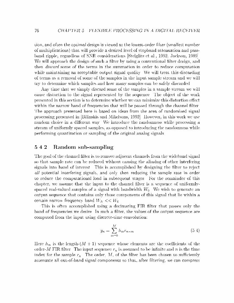
76 CHAPTER 5. FLEXIBLE PROCESSING IN A DIGITAL RECEIVER

tion, and often the optimal design is viewed as the lowest-order �lter (smallest number

of multiplications) that will provide a desired level of stopband attenuation and pass-

band ripple, regardless of SNR considerations [Steiglitz et al., 1992, Jackson, 1989].

We will approach the design of such a �lter by using a conventional �lter design, and

then discard some of the terms in the summation in order to reduce computation

while maintaining an acceptable output signal quality. We will treat this discarding

of terms as a removal of some of the samples in the input sample stream and we will

try to determine which samples and how many samples can be safely discarded.

Any time that we simply discard some of the samples in a sample stream we will

cause distortion to the signal represented by the sequence. The object of the work

presented in this section is to determine whether we can minimize this distortion e�ect

within the narrow band of frequencies that will be passed through the channel �lter.

The approach presented here is based on ideas from the area of randomized signal

processing presented in [Bilinskis and Mikelsons, 1992]. However, in this work we use

random choice in a di�erent way. We introduce the randomness while processing a

stream of uniformly spaced samples, as opposed to introducing the randomness while

performing quantization or sampling of the original analog signals.

5.4.2 Random sub-sampling

The goal of the channel �lter is to remove adjacent channels from the wideband signal

so that sample rate can be reduced without causing the aliasing of other interfering

signals into band of interest. This is accomplished by designing the �lter to reject

all potential interfering signals, and only then reducing the sample rate in order

to reduce the computational load in subsequent stages. For the remainder of this

chapter, we assume that the input to the channel �lter is a sequence of uniformly-

spaced real-valued samples of a signal with bandwidth W0. We wish to generate an

output sequence that contains only those components of this signal that lie within a

certain narrow frequency band WN << W0.

This is often accomplished using a decimating FIR �lter that passes only the

band of frequencies we desire. In such a �lter, the values of the output sequence are

computed from the input using discrete-time convolution:

yn =MXm=0

hmrn�m (5.4)

Here hm is the length-(M + 1) sequence whose elements are the coe�cients of the

order-M FIR �lter. The input sequence rn is assumed to be in�nite and n is the time

index for the sample rn. The order, M , of the �lter has been chosen to su�ciently

attenuate all out-of-band signal components so that, after �ltering, we can compress

5.4. A NEW APPROACH TO BANDWIDTH REDUCTION 77

our representation of the output signal by the decimation factor of D. This need

to resolve and remove out-of-band components is the primary factor that drives the

determination of the minimum length of the �lter response. The compression of the

output representation of the decimating FIR �lter is accomplished as we compute the

output samples only for times n = kD. Each of these output samples will, of course,

require M + 1 multiplications and M additions to compute.

Note that the �lter order M is not chosen speci�cally to provide some required

level of output SNR in the channel �lter. Our idea is to produce output samples y0n

that only approximate the yn to the extent that they still provide the desired level

of SNR at the output while requiring fewer operations to compute. We will compute

these approximate samples by only partially evaluating the summation shown in (5.4)

for each sample:

y0

n=

Xm2Sn

hmrn�m (5.5)

where the selection set Sn � f0; 1; :::;Mg is the subset of the indices of the �lter

coe�cients used to compute yn. We would like to �nd a way to choose this subset that

will adequately approximate the original output sequence yn while using the smallest

amount of computation, that is, using the smallest expected number of terms in each

sum, EfjSnjg.

Our investigation of this problem will begin with the development of some tools

to provide a quantitative understanding of the e�ect of discarding input samples. We

�rst introduce a new model that allows us to analyze the e�ect of discarding di�erent

sets of input samples. We also present an expression that represents the distortion

caused by this operation of discarding samples. Using these tools, we then evaluate an

algorithm that allows us to discard samples while bounding the distortion measured at

the �lter output. This is equivalent to reducing the computation required in channel

separation while maintaining some minimum level of SNR at the �lter output.

The technique that we present has two forms. The �rst makes no assumptions

about the input signal: it simply discard samples randomly to reduce computation.

The other form demonstrates that we can use knowledge about the input signal (not

actual samples, but rather in terms of the expected distribution of energy at di�erent

frequencies) to further reduce computation for the same level of output distortion.

This approach to reducing computation can be generalized in a number of ways, but

in this work we restrict our consideration to a scheme that induces distortion that has

a at spectrum, that is, a type of distortion in which the error at each point in the

sequence is uncorrelated with the error at other sample points. This white distortion

is often easier to deal with in subsequent processing stages, such as a detector.

78 CHAPTER 5. FLEXIBLE PROCESSING IN A DIGITAL RECEIVER

rn

yn

y’n

rn

h n

h n

SampleSelector

nz

(a)

(b)

Figure 5-7: Diagram showing conventional FIR �lter and model for approximating

output samples.

5.4.3 Model for analysis

We will use the model shown in Figure 5-7 to analyze the e�ect of approximating the

output samples through the use of random sub-sampling of the input.

In this �gure we see the original �ltering operation, shown in part (a), as well

as the model that produces the approximate output samples in part (b). In part

(b) the block labeled \Sample Selector" controls which samples will be used in the

computation of the approximate output, y0n. This selection process is modeled as

multiplication by the sequence zn: when a particular zn = 0, the corresponding rn

will not contribute to the computation. The non-zero zn can, in general, take on any

value that will help us reduce the approximation error; we discuss how the values of

the non-zero zn are chosen later. We can now rewrite the expression for the y0nas

y0

n=

MXm=0

hmrn�mzn�m =MX

m=0; zn�m 6=0

hmrn�mzn�m (5.6)

Before we proceed with a complete analysis of this model for sub-sampling and

its e�ects on the �lter output, it is helpful to present a short example of one simple

random sub-sampling scheme. We perform a simple analysis of this example case

to build some intuition for sub-sampling before analyzing a more general rule for

discarding samples in the sections that follow.

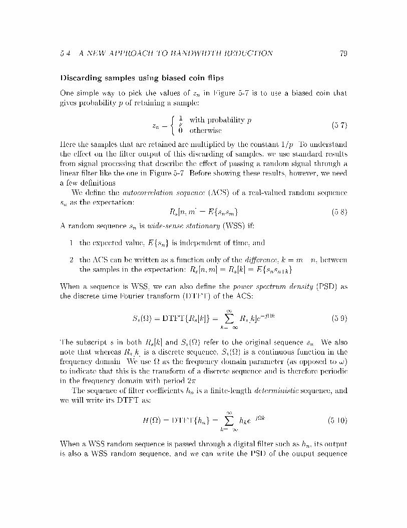
5.4. A NEW APPROACH TO BANDWIDTH REDUCTION 79

Discarding samples using biased coin ips

One simple way to pick the values of zn in Figure 5-7 is to use a biased coin that

gives probability p of retaining a sample:

zn =

(1p

with probability p

0 otherwise(5.7)

Here the samples that are retained are multiplied by the constant 1=p. To understand

the e�ect on the �lter output of this discarding of samples, we use standard results

from signal processing that describe the e�ect of passing a random signal through a

linear �lter like the one in Figure 5-7. Before showing these results, however, we need

a few de�nitions.

We de�ne the autocorrelation sequence (ACS) of a real-valued random sequence

sn as the expectation:

Rs[n;m] = Efsnsmg (5.8)

A random sequence sn is wide-sense stationary (WSS) if:

1. the expected value, Efsng is independent of time, and

2. the ACS can be written as a function only of the di�erence, k = m�n, between

the samples in the expectation: Rs[n;m] = Rs[k] = Efsnsn+kg.

When a sequence is WSS, we can also de�ne the power spectrum density (PSD) as

the discrete time Fourier transform (DTFT) of the ACS:

Ss() = DTFTfRs[k]g =1X

k=�1

Rs[k]e�jk (5.9)

The subscript s in both Rs[k] and Ss() refer to the original sequence sn. We also

note that whereas Rs[k] is a discrete sequence, Ss() is a continuous function in the

frequency domain. We use as the frequency domain parameter (as opposed to !)

to indicate that this is the transform of a discrete sequence and is therefore periodic

in the frequency domain with period 2�.

The sequence of �lter coe�cients hn is a �nite-length deterministic sequence, and

we will write its DTFT as:

H() = DTFTfhng =1X

k=�1

hke�jk (5.10)

When a WSS random sequence is passed through a digital �lter such as hn, its output

is also a WSS random sequence, and we can write the PSD of the output sequence

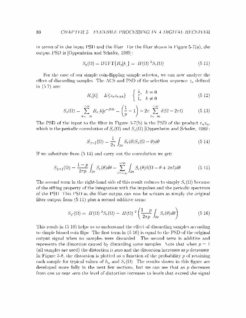
80 CHAPTER 5. FLEXIBLE PROCESSING IN A DIGITAL RECEIVER

in terms of in the input PSD and the �lter. For the �lter shown in Figure 5-7(a), the

output PSD is [Oppenheim and Schafer, 1989]:

Sy() = DTFTfRy[k]g = jH()j2Sr() (5.11)

For the case of our simple coin- ipping sample selector, we can now analyze the

e�ect of discarding samples. The ACS and PSD of the selection sequence zn de�ned

in (5.7) are:

Rz[k] = Efznzn+kg =(

1p; k = 0

1; k 6= 0(5.12)

Sz() =+1X

k=�1

Rz[k]e�jk =

1

p� 1

!+ 2�

+1Xl=�1

�(� 2�l) (5.13)

The PSD of the input to the �lter in Figure 5-7(b) is the PSD of the product rnzn,

which is the periodic convolution of Sr() and Sz() [Oppenheim and Schafer, 1989]:

Sfrzg() =1

2�

Z2�Sr(�)Sz(� �)d� (5.14)

If we substitute from (5.13) and carry out the convolution we get:

Sfrzg() =1� p

2�p

Z2�Sr(�)d� +

+1Xl=�1

Z2�Sr(�)�(� � + 2�l)d� (5.15)

The second term in the right-hand side of this result reduces to simply Sr() because

of the sifting property of the integration with the impulses and the periodic spectrum

of the PSD. This PSD at the �lter output can now be written as simply the original

�lter output from (5.11) plus a second additive term:

Sy0() = jH()j2Sr() + jH()j2 1� p

2�p

Z2�Sr(�)d�

!(5.16)

This result in (5.16) helps us to understand the e�ect of discarding samples according

to simple biased coin ips. The �rst term in (5.16) is equal to the PSD of the original

output signal when no samples were discarded. The second term is additive and

represents the distortion caused by discarding some samples. Note that when p = 1

(all samples are used) the distortion is zero and the distortion increases as p decreases.

In Figure 5-8, the distortion is plotted as a function of the probability p of retaining

each sample for typical values of hn and Sr(). The results shown in this �gure are

developed more fully in the next few sections, but we can see that as p decreases

from one to near zero the level of distortion increases to levels that exceed the signal

5.4. A NEW APPROACH TO BANDWIDTH REDUCTION 81

-30

-25

-20

-15

-10

-5

0

0 0.2 0.4 0.6 0.8 1

Dis

tort

ion

(in d

B r

elat

ive

to R

ecei

ved

Sig

nal P

ower

)

Fraction of Input Samples Used (p)

Figure 5-8: Distortion due to discarding input samples according to random coin ips.

of interest (at 0 dB in the plot, the power of the distortion equals the power of the

signal itself).

Analysis of the error sequence

The example of choosing the values of zn using a biased coin helped us to gain some

intuition about the e�ect of discarding input samples as we compute the output of

a narrowband channel �lter. Discarding samples led to additive distortion in (5.16)

whose PSD increased in magnitude as samples were discarded. In order to understand

how to choose the selection sequence zn in a manner that will allow us to more carefully

control the induced distortion, we now provide a more general analysis the e�ect of

discarding samples.

We �rst de�ne the error between the approximate �lter output y0nand the original

output sequence:

en = y0

n� yn (5.17)

We would like this error sequence, en, to have zero mean (to provide an unbiased

approximation) and, for a given choice of the sequence zn, we would like to compute

its variance, i.e., the mean-squared error (MSE) of the distorted output sequence

relative to the original output:

var(en) = Efe2ng (5.18)

82 CHAPTER 5. FLEXIBLE PROCESSING IN A DIGITAL RECEIVER

rn

z n

d n

h n

e n+

-

Figure 5-9: Model for analysis of error variance due to random sub-sampling.

In Figure 5-9, we have combined the two schemes from Figure 5-7 to produce

the error sequence for the purpose of analysis. Before using this combined model to

derive the relationship between the input sequences and the output variance, we need

to state a few assumptions that will simplify the derivation.

We again assume that the input sequence rn is wide-sense stationary. We also

assume that the zn are chosen independently of the values of rn. This allows us

to fully realize the computational savings of discarding some input samples without

examination, as well as allowing us to pre-compute zn. It is important that the

sequence zn have a non-zero mean; we will see later that this determines the amplitude

of the desired signal in the output sequence. Without loss of generality, we assume

that Efzng = 1. This speci�c choice prevents problems with scaling factors later but

does not limit our choice of sequences, as long as we scale them appropriately. We

also will de�ne vn = zn � 1 to simplify the notation in our analysis (so Efvng = 0).

We can now write the ACS for the �lter input sequence, dn = rnzn�rn (the distortionsequence), as:

Rd[k] = Efdndn+kg = Efrnrn+kvnvn+kg = Rr[k]Rv[k] (5.19)

Our model for approximating the �ltering operation has several desirable char-

acteristics. First, if the length of the �lter (M + 1 coe�cients) is greater than the

decimation factor, then some input sample will be required in the computation of

multiple output values. When this is the case, our model will ensure that these sam-

ples are used in every such computation or in none of them. This is useful in a real

implementation where much of the cost of the computation is retrieving a sample

from memory, not in performing the actual arithmetic operation (hmrn�m).

In a sense, we are approximating the input sequence as opposed to approximating

the �lter. The selection set Sn can be viewed as the set of �lter coe�cients that are

5.4. A NEW APPROACH TO BANDWIDTH REDUCTION 83

used to compute each output. If this set were the same for every n, it would simply

de�ne a new �lter that is an approximation of the original �lter. This approximation

approach could be evaluated using standard �lter response techniques and the analysis

of such an approach is not part of this work.

Problem Statement

Using the model shown in Figure 5-9 and the de�nitions above, we now state our

problem more precisely:

Find the sequence zn that minimizes the expected amount of computation

required to approximate the �lter output while ensuring that the error

variance is less than or equal to a bound B:

min [Prfzn 6= 0g] such that Efe2ng � B (5.20)

Finding the Error Variance

To analyze the e�ects of zn on the variance of the error sequence, we �rst write the

power spectrum density of the output of the �lter in Figure 5-9. This output PSD

can be written in terms of the input PSD and the frequency response of the �lter,

similar to (5.11):

Se() = jH()j2 Sd() (5.21)

The variance of en can be written as the inverse DTFT of this PSD evaluated at

k = 0:

var(en) = Re[0] =

�1

2�

Z2�Se()e

�jkd

�k=0

=1

2�

Z2�Se()d (5.22)

Writing this variance in terms of the input sequence PSD:

var(en) =1

2�

Z2�jH()j2 Sd()d (5.23)

The PSD of the input sequence, Sd(), represents the distribution in frequency of

the expected distortion (the squared di�erence, d2n) caused by discarding samples

according to the sequence zn. To reduce the variance at the output we would ideally

like this distortion to occur at frequencies for which the amplitude of H() in (5.23)is

small: the stopband of the �lter. If dn is a white sequence then Sd() will be constant

for all (since dn must also be zero-mean). This implies, from (5.23), that the

output variance will be simply proportional to the input variance, Efd2ng, and that

84 CHAPTER 5. FLEXIBLE PROCESSING IN A DIGITAL RECEIVER

the proportionality factor will depend only on the response of the bandpass �lter,

H().

If we substitute in (5.23) using the de�nition of the DTFT of Rd[k],

var(en) =1

2�

Z2�jH()j2

24 1Xk=�1

Rd[k]e�jk

35 d (5.24)

Exchanging the order of summation and integration, we get:

var(en) =1X

k=�1

Rd[k]

�1

2�

Z2�jH()j2 e�jkd

�(5.25)

The expression in the square brackets above is the inverse DTFT of the squared

response of the �lter. This can be written as the ACS of the deterministic, �nite-

length sequence of �lter coe�cients hn, which we will call ch[k]:

ch[k] =1X

m=�1

h[m]h[k +m] =1

2�

Z2�jH()j2 e�jkd (5.26)

We can now combine all of these results to show that the output error variance is

simply the sum of a product of three sequences:

var(en) =1X

k=�1

Rr[k]Rv[k]c[k] =1X

k=�1

Rr[k](Rz[k]� 1)ch[k] (5.27)

To check this result, consider the case of zero output distortion: choosing zn = 1 for

all n results in Rv[k] = 0 for all k, giving zero error.

This result in (5.27) is signi�cant for several reasons. First, it shows that the

error variance of our approximation scheme depends on the sequence vn (and hence

zn) only through its ACS. Second, it shows that the error variance depends linearly

on all three of the key parts of the system: the ACS of the input sequence, the ACS

of the selection sequence and the coe�cients of the channel selection �lter.

Finding a Good Selection Sequence

We can now begin to look at how (5.27) helps us choose the selection sequence zn,

minimizing the amount of computation to produce an output with a speci�ed bounded

variance. This sequence will have the following properties:

1. It provides a bounded error variance, given by (5.27).

5.4. A NEW APPROACH TO BANDWIDTH REDUCTION 85

SequenceTransform

x n

z n

ng

h n

wn

rn y’n

Offline

Figure 5-10: Random sub-sampling using a transformed sequence for sample selection.

2. It allows us to discard as many samples as possible, that is to maximize the

probability that zn = 0, subject to property (1) above.

3. It produces a distortion with uncorrelated error values at each point in the

sequence.

We now identify two separate cases as we try to decide which samples to discard.

In (5.27), we saw that the induced error variance depended only on the ACS of

the received wideband sequence and the ACS of the channel �lter. Although it is

conceivable that in some cases we may have a good idea of the spectral distribution of

the received signal (and therefore its ACS), we may not always have this information.

We therefore identify two cases as we try to �nd a good choice for the selection

sequence, zn.

Although it is well known how to generate a random sequence with a desired ACS

(e.g. by generating \shaped noise", see [Stark and Woods, 1986]), we found no prior

work on how to directly generate such a sequence with a relatively high probability

that zn = 0. Instead, we will start with a candidate selection sequence, xn, that has

a desirable ACS and perform a sequence transformation to convert it to a sequence

zn that has more zero elements and an ACS that remains \close" to that of xn, i.e.

Rz[k] � Rx[k]. This sequence transformation approach is shown in Figure 5-10, which

also depicts the creation of the initial sequence xn by the �ltering of a white noise

sequence wn with the shaping �lter gn. We will describe how the �lter gn is chosen

in a later section.

In terms of our transformation scheme, the error variance of (5.27) can be written

as two components: one component due to choice of the original sequence xn (the

�rst term below), and another to the transforming e�ect that introduces more zeros

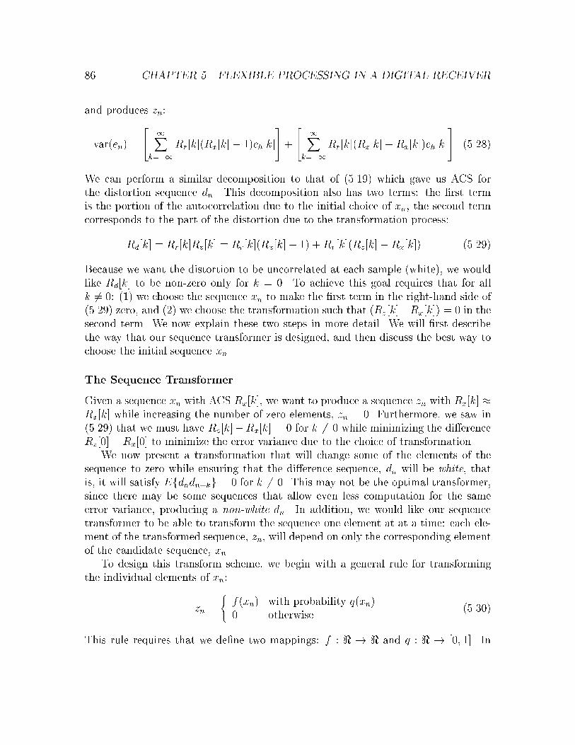
86 CHAPTER 5. FLEXIBLE PROCESSING IN A DIGITAL RECEIVER

and produces zn:

var(en) =

24 1Xk=�1

Rr[k](Rx[k]� 1)ch[k]

35 +

24 1Xk=�1

Rr[k](Rz[k]� Rx[k])ch[k]

35 (5.28)

We can perform a similar decomposition to that of (5.19) which gave us ACS for

the distortion sequence dn. This decomposition also has two terms: the �rst term

is the portion of the autocorrelation due to the initial choice of xn, the second term

corresponds to the part of the distortion due to the transformation process:

Rd[k] = Rr[k]Rv[k] = Rr[k](Rx[k]� 1) +Rr[k](Rz[k]� Rx[k]) (5.29)

Because we want the distortion to be uncorrelated at each sample (white), we would

like Rd[k] to be non-zero only for k = 0. To achieve this goal requires that for all

k 6= 0: (1) we choose the sequence xn to make the �rst term in the right-hand side of

(5.29) zero, and (2) we choose the transformation such that (Rz[k]�Rx[k]) = 0 in the

second term. We now explain these two steps in more detail. We will �rst describe

the way that our sequence transformer is designed, and then discuss the best way to

choose the initial sequence xn.

The Sequence Transformer

Given a sequence xn with ACS Rx[k], we want to produce a sequence zn with Rz[k] �Rx[k] while increasing the number of zero elements, zn = 0. Furthermore, we saw in

(5.29) that we must have Rz[k]�Rx[k] = 0 for k 6= 0 while minimizing the di�erence

Rz[0]� Rx[0] to minimize the error variance due to the choice of transformation.

We now present a transformation that will change some of the elements of the

sequence to zero while ensuring that the di�erence sequence, dn will be white, that

is, it will satisfy Efdndn+kg = 0 for k 6= 0. This may not be the optimal transformer,

since there may be some sequences that allow even less computation for the same

error variance, producing a non-white dn. In addition, we would like our sequence

transformer to be able to transform the sequence one element at at a time: each ele-

ment of the transformed sequence, zn, will depend on only the corresponding element

of the candidate sequence, xn.

To design this transform scheme, we begin with a general rule for transforming

the individual elements of xn:

zn =

(f(xn) with probability q(xn)

0 otherwise(5.30)

This rule requires that we de�ne two mappings: f : < ! < and q : < ! [0; 1]. In

5.4. A NEW APPROACH TO BANDWIDTH REDUCTION 87

choosing f and q to accomplish our goals, we �rst compute the ACS of the transformed

sequence zn. For the case k 6= 0 we have

Efznzn+kg =Z1

�1

Z1

�1

znzn+kp(zn; zn+k)dzndzn+k

=Z1

�1

Z1

�1

f(xn)q(xn)f(xn+k)q(xn+k)p(xn; xn+k)dxndxn+k (5.31)

To ensure that Efznzn+kg = Efxnxn+kg for k 6= 0, we now choose f(xn) = xn=q(xn),

giving:

Efznzn+kg =Z1

�1

Z1

�1

xnxn+kp(xn; xn+k)dxndxn+k = Efxnxn+kg (5.32)

A similar computation allows us to �nd Rz[0]:

Rz[0] = Efz2ng =

Z1

�1

x2n

q(xn)p(xn)dxn = E

(x2n

q(xn)

)(5.33)

Now, since 0 � q(xn) � 1, it is clear that Rz[0] � Rx[0], with equality only in the

case where q(xn) = 1, for all values of xn that occur with non-zero probability. This

implies that anytime Prfq(xn) < 1g > 0, our sequence transformer will induce some

non-zero output distortion as seen in the second term of (5.28). We wish to �nd the

function q that minimizes the expected computation (minimizes Prfzn 6= 0g) for agiven bounded output distortion, var(en).

To simplify the problem of �nding the best q, we assume that the xn are drawn

from a discrete distribution: xn 2 X (and therefore zn 2 Z). This simpli�cation will

allow us to solve a discrete optimization problem to �nd the best choice for q(xn) and

does not signi�cantly a�ect the eventual result. We use the notation xi to indicate an

element of the set X and we refer to the probability mass function over these values

using pi, that is Prfxn = xig = pi. We will also use the notation qi to refer to the

values of function q(xn), that is q(xn) = qi when xn = xi. So we now have f : X ! Zand q : X ! [0; 1].

In order to ensure Rz[k] = Rx[k] for k 6= 0, we choose f(xi) = xi=qi, and (5.33)

now becomes Rz[0] = Efx2i=qig when we use a discrete distribution for xn.

At this point, �nding the best choice for the function qi can be written as an

optimization problem. The goal is to choose the values of qi providing the highest

probability of zn = 0 (lowest probability that zn 6= 0) given a bounded distortion for

the transformer:

88 CHAPTER 5. FLEXIBLE PROCESSING IN A DIGITAL RECEIVER

Problem Statement

Find qi to give

min

"Xi

piqi

#such that Efx2

i=qig =

Xi

pix2i

qi� � (5.34)

Note that although the value we actually need to bound is Rz[0]�Rx[0] = Efx2i=qig�

Efx2ig, since both terms in the di�erence are positive and Efx2

ig is �xed for the given

sequence xn, we can equivalently bound the �rst term alone.

Solution

We can assume that equality holds in the constraint above at any optimal solution;

otherwise we would be able to increase one of the qi to achieve equality, thereby

reducing the sum to be minimized. This constraint is a hyperbolic surface in the

qis and since all of the parameters are non-negative, this is a convex surface. The

convexity implies that there exists a single global minimum point on the constraint

surface. Any global solution to this constrained minimization in (5.34) will also satisfy

pair-wise optimality for the individual pis. That is, the same global solution will also

satisfy:

min

�piqi + pjqj

�such that

pix2i

qi+pjx

2j

qj= �ij (5.35)

for some �xed �ij for all i 6= j. If this were not so, then we would be able to improve

on the global optimum. Because of this pairwise optimality condition, we can solve

the pairwise problem by eliminating qj through substitution in the above, setting the

derivative equal to zero and �nding the optimal qi (and qj by symmetry):

qi =1

�ijjxij

�pijxij+ pjjxjj

�(5.36)

These relationships allow us to show that the ratio qi=qj does not depend on �ij:

qi=qj = jxij=jxjj. From here we can easily �nd the global solution:

qi = jxij Efjxnjg

�

!(5.37)

This result for the values of qi is not quite complete. If any of the xi are such that

jxij > �=Efjxnjg this would result in a value of qi that is greater than one, which

would be unacceptable for a probability value. For such xi, the optimal solution is

to choose qi = 1, so that such values will never be changed as we transform the se-

5.4. A NEW APPROACH TO BANDWIDTH REDUCTION 89

quence xn into zn. The intuition here is that these are the outlying values of xi in the

distribution, and changing these values with non-zero probability causes more distor-

tion than simply changing the values of smaller-magnitude xi with higher probability.

Only those with smaller jxij are subject to possible transformation according to (5.30)

and in the limit as � ! Efx2ng none of the xis will be subject to rounding. In this

case we will not be able to transform any elements to zero, but will have zn = xn; 8nin order to satisfy the bound on distortion. To capture this e�ect, we de�ne the set SRas those xi that will be subject to being transformed with non-zero probability, that

is, those xi such that jxij < �=Efjxnjg. The �nal rule for our sequence transformer

is now:

zn =

(xn=q(xn) with probability q(xn)

0 with probability 1� q(xn)(5.38)

Where the values of q(xn) are given by:

q(xn) = qi for xn = xi; where qi =

(1 if xi =2 SRjxij

�Efjxnjg

�

�if xi 2 SR

(5.39)

The set SR consists of xi that are subject to rounding (those xi for which qi < 1) are

those for which:

SR : xi such that jxij <�

Efjxnjg(5.40)

5.4.4 Analytical evaluation of the sequence transformer

Before analyzing the results above, it is helpful to review the overall goal of our

random sub-sampling scheme, which is to approximate the output of narrowband

channel selection �lter by using only a subset of the input samples. The particular

approach of using a selection sequence to model the e�ect of sub-sampling is motivated

by the high costs of memory retrieval relative to multiplication operations. The idea is

to use a selection sequence zn so that those samples not discarded could be multiplied

by some non-zero value to reduce the e�ect of sub-sampling.

Our analysis showed that MSE distortion due to sub-sampling depends on the ACS

of selection sequence. There is no known prior work on generating such a sequence

with large proportion of zeros, we therefore decided to use a two-step approach:

choose a candidate sequence, xn, that has desired ACS, followed by a transformation

that would increase the number of zero elements. As we evaluate the performance of

the sequence transformer, we must keep in mind that this approach is not the entire

solution to our main problem of minimizing the computation for a channel �lter in

a digital receiver through sub-sampling the input, as de�ned by (5.20). In general,

there may be an entire class of sequences that cannot be generated through our two-

90 CHAPTER 5. FLEXIBLE PROCESSING IN A DIGITAL RECEIVER

step approach, yet provide superior performance when used to select which samples

should be discarded in our random sub-sampling approach. This being said, we now

analyze the performance of our sequence transformation scheme.

The performance of the sequence transformer can be measured by determining how

much it is able to reduce the cost of computing the �lter output for a given bound on

error variance. This cost reduction is simply the probability that a particular element

of the input sequence will be discarded:

Prfzn = 0g = Ef1� q(xn)g =Xi

pi(1� qi) (5.41)

Substituting the expression for qi from (5.39), we can write the complement of this,

the amount of computation required:

Prfzn 6= 0g =Xi

piqi =Efjxnjg

�

Xi: xi2SR

pijxij+X

i: xi =2SR

pi (5.42)

We can use this result to compare the two cases that we identi�ed earlier to see if

having knowledge of the received wideband signal and the �lter response can help to

reduce computation.

Case I: Autocorrelation of received sequence is unknown

In the �rst case, we assume no knowledge of the ACS of the received sequence rn.

We recall that the error variance given in (5.28) had two components. The �rst of

these is due to the choice of xn. Because we do not know Rr[k], it is reasonable to

choose xn = 1 for all n. This will give zero distortion due to the �rst term (since

we will have Rx[k] = 1; 8k). The distortion due to the transformation, the second

term in (5.28), is simply Rr[0](Rz[0] � Rx[0])ch[0]. For our sequence xn we have a

trivial distribution, xn = 1 with probability one. For a given amount B of allowable

distortion in this case, we have:

var(en) = Rr[0](Rz[0]� Rx[0])ch[0] = Rr[0](�1 � 1)ch[0] = B (5.43)

�1 =B

Rr[0]ch[0]+ 1 (5.44)

The transformer reduces to the simple case:

zn =

(�1 with probability 1

�1

0 otherwise(5.45)

5.4. A NEW APPROACH TO BANDWIDTH REDUCTION 91

Using this rule, we will always have xi < �1=Efjxnjg = �1, so the expected computa-

tion is:

Prfzn 6= 0g =1

�1(5.46)

This case where the candidate sequence is chosen as xn = 1 for all n corresponds

to the simple case of using a biased coin that we discussed earlier in this chapter,

although is is now clear how we should pick the probability p = 1=�1 to achieve a

desired level of error. We will perform further analysis on these results in the next

section to provide more insight on the e�ectiveness of this scheme for this case and

the next.

Case II: Autocorrelation of received sequence is known

In this case, we assume that the ACS of the received sequence rn is known. The �rst

term of the error variance given in (5.28) was zero in Case I, but here we consider

that we can �nd a non-trivial sequence xn that will make this term small (or even

zero), so let � =P

kRr[k](Rx[k]� 1)ch[k]. The total distortion for this case is now

var(en) = � +Rr[0](�2 � Rx[0])ch[0] = B (5.47)

�2 =B � �

Rr[0]ch[0]+Rx[0] = �1 + var(xn)�

�

Rr[0]ch[0](5.48)

The transformer is:

zn =

8><>:

xn if xn =2 SR�2

Efjxnjg� Sign(xn) with probability jxnj��1

2 Efjxnjg if xn 2 SR0 otherwise

(5.49)

Using this rule, the expected computation from (5.42) is:

Prfzn 6= 0g = Efjxnjg

�2

! Xi: xi2SR

pijxij+X

i: xi =2SR

pi (5.50)

Comparison of Cases I and II

At this point we have produced results that show the expected amount of computation

that is required to produce the approximate �lter output for two di�erent cases. To

determine whether the second case is able to improve on the performance of the �rst,

we simply need to see which can produce an output with the same bounded error

variance using less computation.

92 CHAPTER 5. FLEXIBLE PROCESSING IN A DIGITAL RECEIVER

As we consider the above results, we will need to understand the e�ect of the

Efjxnjg term that appears in (5.50). We do so in the context of our approach which

generates xn using an FIR �lter to shape the spectrum of a white sequence, as in

Figure 5-10. Here xn has an ACS that is determined by the response of the �lter gn,

which itself is determined from (5.28) in order to minimize �. When we generate xnusing an FIR �lter, each sample of xn will be the weighted sum of a large number

of independent samples of the white sequence wn. This will tend to produce samples

of xn that have a Gaussian distribution. When we consider (5.50), we see that for

a Gaussian distribution with mean Efxng = 1 (because zn must also have unit

mean and the transformer preserves the mean), Efjxnjg is strictly greater than one.

Although Efjxnjg > 1, it is not much greater if the variance of xn is relatively small

so that the negative tail the distribution of xn (the part a�ected by the absolute value

operation) has a small area.

To get a qualitative feel for the relative performance of the two cases, we can

now compare the results of (5.46) and (5.50). We consider the case of values of the

bound B on the variance of the error in (5.20) for which most of the xi are subject

to rounding, that is, xi 2 SR for most xi. In this case, the second summation in

(5.50) will be very small and the �rst summation will be approximately equal to

Efjxnjg � 1. We will then have Prfzn 6= 0g � 1=�2. Furthermore, if we assume that

� in (5.48) is small, the we see that a non-zero variance for xn will lead to �2 > �1 and

thus to an improvement in performance for case II relative to case I. To achieve this

improved performance, however, we need to �nd a general solution which allows us to

determine an ACS for a candidate sequence xn with non-zero variance in addition to

a small (or zero) resulting value for �, the �rst term in (5.28). This general solution

is the goal of on-going work.

In the next section, we present the result of computer simulations that validate the

results of (5.46) and provide a more concrete comparison of the two di�erent cases.

5.5 Evaluation of Random Sub-sampling

Figure 5-11 shows the results of computer simulations that validate the performance

of the sequence transformer analysis for the case where the autocorrelation is not

known (Case I). In these simulations, randomWSS signals were generated to represent

the received signal. A selection sequence zn was produced to simulate independent

random rounding decisions according to the transformation rule in (5.45). In the

�gure, the solid lines represent the result of (5.46) plotted for speci�c values of Rr[0]

and ch[0] over a range of values for B, in dB relative to the power of the received

signal. The individual points on the plot are the measured results of the error variance

produced when sub-sampling the random signal by zeroing speci�c proportions of the

5.5. EVALUATION OF RANDOM SUB-SAMPLING 93

-30

-25

-20

-15

-10

-5

0

0.5 0.55 0.6 0.65 0.7 0.75 0.8 0.85 0.9 0.95 1

Err

or V

aria

nce

(in d

B r

elat

ive

to R

ecei

ved

Sig

nal P

ower

)

Fraction of Input Samples Used

BW = 40%

BW = 20%

BW = 10%

BW = 4%

BW = 2%

-30

-25

-20

-15

-10

-5

0

0.5 0.55 0.6 0.65 0.7 0.75 0.8 0.85 0.9 0.95 1

Err

or V

aria

nce

(in d

B r

elat

ive

to R

ecei

ved

Sig

nal P

ower

)

Fraction of Input Samples Used

BW = 40%

BW = 20%

BW = 10%

BW = 4%

BW = 2%

Figure 5-11: Output error variance relative to desired signal power versus proportion

of input samples used for several cases of output signal relative bandwidth.

input samples. The plot shows results for �ve di�erent values of ch[0], corresponding

to di�erent bandwidths for the desired signal relative to the wideband input. The

results show that if we need to bound the distortion at some level, say �15dB relative

to the received signal, the approach of Case I would provide some reasonable reduction

in computation. The results shown are for the base case where there are no interfering

signals in adjacent channels and all of the signal energy is in the desired band. If any

other signals are present in the wideband input signal, the respective curves would

shift upward to re ect the increased value of Rr[0], the input signal variance.

A contrast between the approach of Case I and an alternative, a uniform sub-

sampling scheme, is their behavior in the presence of interference. The qualitative

e�ect of the random sub-sampling approach is to provide more uniform behavior,

regardless of the location of any interfering signals relative to the desired signal.

For example, consider the case where a single interfering signal is present in the

stopband of the channel �lter. For the random sub-sampling approach, this would

result in an upward shift of the curves in Figure 5-11 by 3 dB when the interferer is

independent of the desired signal and has equal power (so Rr[0] will be twice as much

94 CHAPTER 5. FLEXIBLE PROCESSING IN A DIGITAL RECEIVER

as with no interferer present). This result does not depend on the location of the

interferer within the stopband: the interfering signal could have a center frequency

anywhere in the stopband and the result would be additive uncorrelated distortion at

about -15 dB relative to the desired signal (using half of the samples with a relative

bandwidth of 2% in Figure 5-11).

If half of the samples are instead chosen uniformly, this is equivalent to decimation

by a factor of two prior to �ltering. The resulting e�ect would depend on the relative

frequencies of the desired signal and the interferer. The interfering signal might be

aliased into the stopband of the �lter, resulting in negligible distortion. On the other

hand, it is possible that the interferer would be aliased into the passband of the �lter

by the decimation, and this would result in signi�cant distortion at the �lter output

(zero dB relative to the desired signal).

It is also interesting to note the di�erence between the individual curves in Fig-

ure 5-11 for the di�erent relative bandwidths of the output signal. These curves show

that there is smaller error variance when the bandwidth of the output signal is more

narrow relative to the input bandwidth. This observation leads to a more general and

important conclusion about the results of (5.46) and (5.50), which is that the amount

of computation required to separate a narrowband signal with a �xed level of output

distortion need not depend on the input bandwidth, but rather on output bandwidth

and the amount of interference in the stopband.

For example, consider the case of a narrowband lowpass channel separation �lter.

If we increase the input sample rate while the output sample rate is held constant,

the sum of the coe�cients hn will remain constant to provide constant gain at center

of the passband (zero frequency). The number of coe�cient in the �lter, however, will

increase in proportion to the increasing input bandwidth because its response must

span a constant interval of time (and the sample interval Ts will decrease as the input

bandwidth increases). The value of ch[0] is the sum of the squared coe�cients, ch[0] =PM

n=0 h2n, and this will decrease in inverse proportion to an increasing input sample

rate. From (5.43), we conclude that the computation, CNB, required to separate the

narrowband channel will thus remain constant if a �xed level of distortion (B) is

speci�ed in the output:

CNB = PRfzn 6= 0g � fLength of �lterg � Constant as

�Rin

Rout

�increases (5.51)

Although the amount of computation required for the channel �ltering does not

depend directly on the input sample rate, this amount does depend on the amount

of interference present in the stopband. From (5.43) we see that if more interfering

signals are present, the variance of the input signal, Rr[0], will increase, resulting

in an increasing amount of computation required to maintain a �xed level of output

5.5. EVALUATION OF RANDOM SUB-SAMPLING 95

-30

-25

-20

-15

-10

-5

0

0 0.2 0.4 0.6 0.8 1

Err

or V

aria

nce

(in d

B r

elat

ive

to R

ecei

ved

Sig

nal P

ower

)

Fraction of Input Samples Used

var(x)=1

var(x)=4

var(x)=2-> var(x)=.25

Case I

-30

-25

-20

-15

-10

-5

0

0 0.2 0.4 0.6 0.8 1

Err

or V

aria

nce

(in d

B r

elat

ive

to R

ecei

ved

Sig

nal P

ower

)

Fraction of Input Samples Used

var(x)=1

var(x)=4

var(x)=2-> var(x)=.25

Case I

Figure 5-12: Comparison of Case I and Case II results for three values of var(xn).

error variance, B.

In Figure 5-12, we show a comparison of the performance for the two di�erent

cases. This plot shows a comparison of the results for cases I and II from (5.46)

and (5.50) for several di�erent values of Rx[0] under the assumption that � = 0 and

the output signal bandwidth is 10% of the input bandwidth. Here we see that using

a candidate sequence with a non-zero variance can further reduce the proportion of

samples required to produce an output signal with a bounded error variance. As

in the previous case, this plot shows the base case where all of the received signal

power is assumed to be in-band, any interfering signals present in the stopband of

the �lter would result in an upward shift in each of the curves. The curves show that

at low levels of distortion (less than -15 dB), increasing the variance of the candidate

sequence reduces the computation required to produce a �xed quality output only to

a point (when var(xn � 2), beyond which a further increase in variance is not helpful.

96 CHAPTER 5. FLEXIBLE PROCESSING IN A DIGITAL RECEIVER

5.6 Summary

In this chapter, we have addressed the two di�erent steps of the channel selection

process: frequency translation and bandwidth reduction through �ltering. For fre-

quency translation, the conventional approach provides excessive exibility in fre-

quency translation, but at the cost of signi�cant excess computation. We have demon-

strated how to perform the same function using a composite �lter followed by �nal

translation at the low output sample rate after �ltering, this enabling the computa-

tion of the frequency translation step to be made proportional to the output sample

rate.

We have also describes an unnecessary coupling that exists between the length

of the �lter response and the number of input samples used when computing the

output of a narrowband channel separating �lter using conventional approaches. In

order to provide adequate out-of-band rejection, it may incur unnecessary computa-

tion by processing excessive samples. Instead, we have demonstrated that we can

independently control �lter response and output SNR.

We control output SNR by bounding the distortion caused by approximating

the input signal through random sub-sampling. We then can perform bandwidth

reduction using a relatively small number of input samples while maintaining the

desired output SNR. This reduced number of samples reduces the number of memory

accesses required to retrieve data, at the cost of potentially performing an additional

multiplication for each input sample used. The two-step approach presented here

utilizes a sequence transformer to produce white additive distortion (noise) at the

output, although it is conceivable that a more general approach can be developed

that provides greater computation reduction using non-white distortion.

Chapter 6

Data Symbol Detection

The job of the channel decoder is to analyze the signal recovered from the channel

in order to determine the original bits that were sent by the transmitter. In the

previous chapter, we described this process as a many-to-one mapping since there

are many ways that the channel can corrupt the transmitted waveform sensed by

the receiver, and the receiver must map each of these corrupted versions back to the

original discrete data. We have already shown how the process of channel separation

deals with the part of the channel distortion caused by interfering signals in other

frequency bands. In this chapter, we will examine the second step of the process,

detection.

We begin with an overview of the detection process, emphasizing the relationship

between the input samples and the symbol to be estimated. We then review one

widely-used approach to detection that relies on a special property of certain pulse

shapes enabling us to make optimal symbol-by-symbol decisions. We then spend the

remainder of the chapter describing a new approach to detection that enables the

system to adapt the detector to e�ciently provide a speci�ed level of performance for

existing channel conditions.

6.1 Overview: Symbol Detection

After channel separation has been completed, the receiver must make decisions about

the individual symbols encoded in the received waveform. The sequence of processing

steps in the receiver is shown in �gure 6-1: in this �gure, the symbol detector is

divided into two di�erent tasks, synchronization and detection. Synchronization is

the process of determining the speci�c set of received samples that correspond to

each particular symbol to be detected. The job of the detector is then to analyze the

speci�c section of the received waveform that corresponds to a particular symbol and

97

98 CHAPTER 6. DATA SYMBOL DETECTION

ChannelSeparation

SourceDecoderDecoder

ErrorUserChannel

Detection

Channel Decoder

Symbol Detection

Synchronization

Figure 6-1: Diagram of the channel decoder showing division of the symbol detector

into synchronization and detection steps.

decide which is the most likely corresponding data symbol. In this chapter, we focus

on the detection process under the assumption that the required synchronization has

been accomplished. A more detailed discussion of techniques for synchronization in

digital receivers is available in [Meyr et al., 1997].

The output of the detection process is the sequence of symbols that the receiver

believes was originally transmitted. This sequence is passed to the error decoder,

which will either correct those errors it can, or simply detect errors and take other

appropriate actions. It is in this context of protecting against errors in the receiver

that the overall role of the detector in the system becomes clear. In a noisy envi-

ronment, the detector will always produce some errors. One of the functions of the

receiver as a whole is to control the level of errors through various mechanisms to

ensure that end user sees only an acceptable level of errors. These mechanisms are

not limited to the detector, or even the channel decoder, but include redundancy

at higher layers in the communication system or other techniques such as protocols

for retransmission. To design an e�cient and exible system, we need to provide

the required error performance in a way that e�ciently uses the available system

resources.

When seen in this light, the detector does not necessarily need to produce an

optimal estimate of the received symbols in every situation. Rather, it needs to recover

symbols in such a way that the required error performance is e�ciently achieved

through the composite behavior of all the error control mechanisms. Figure 6-2 shows

a typical performance curve for an optimal digital detector. In this plot, we see that

the probability of bit errors depends on the SNR of the received signal. If a particular

system is designed such that the detector needs to achieve a bit error rate (BER) of

10�4 at some worst-case SNR, say 8.5 dB SNR, then it will provide much better BER

6.2. CONVENTIONAL APPROACH TO DETECTION 99

1e-09

1e-08

1e-07

1e-06

1e-05

0.0001

0.001

0.01

0.1

0 2 4 6 8 10 12

Bit

Err

or R

ate

SNR (dB)

Figure 6-2: Plot of bit-error rate versus SNR for a two level PAM system.

if the SNR is higher. For example, if the system is experiencing an SNR of 11 dB then

the optimal detector will produce a BER of 10�6. This extra performance will not

hurt the overall system performance, but if it is achieved at the cost of unnecessary

resource consumption, then it will not be the most e�cient solution.

In this chapter we will present an approach that enables the detector to e�ciently

provide a desired level of BER for a speci�c SNR from current channel conditions. Be-

fore presenting these results, we �rst review some conventional techniques to perform

detection and try to develop an understanding of how this process can be modi�ed

to provide e�cient and controllable performance trade-o�s.

6.2 Conventional Approach to Detection

Conventional approaches to detection depend heavily on the type of distortion expe-

rienced in the wireless channel. In some cases multi-path reception causes a situation

where a speci�c symbol in the encoded waveform is distorted by other preceding or

following symbols. In such a case, symbol-by-symbol detection is not feasible, but

the receiver must, in a sense, simultaneously estimate an entire sequence of symbols

because of the inter-symbol interference (ISI) e�ects. We will not consider this case

in the present work, but will consider the case of a system that experiences additive

100 CHAPTER 6. DATA SYMBOL DETECTION

noise. We will consider this case in the context of a system that has limited RF

spectrum available and needs to e�ciently use this limited bandwidth to achieve the

best possible data rate.

As we consider some standard approaches to this problem, we will review how the

system can use pulse shaping techniques to e�ectively use its spectrum as well as the

concept of the matched �lter detector.

6.2.1 The design of pulses for digital modulation

In chapter 4 we discussed how to synthesize waveforms that encode sequences of

symbols into a continuous waveform. We noted that each symbol can be encoded

with a shaped pulse and then time-shifted pulses added together to form continuous

waveform. At the same time we saw that these pulses often overlap. As we try

to recover the values of original data symbols, we need to somehow separate the

original pulse shapes that were added together. One common way to make this

separation possible is to use pulses that satisfy the Nyquist Criterion for zero inter-

symbol interference (ISI) [Lee and Messerschmitt, 1994].

This criterion ensures that for each encoded symbol there will be one instant in

time when the contributions in the composite waveform from all adjacent pulses will

be zero (although there will still be noise present in the received waveform). Such a

pulse shape is shown in �gure 6-3, part (a). In part (b) of this �gure are a series of

eight scaled and time shifted pulses that encode eight consecutive data symbols, and

in part (c) is the composite waveform, the sum of the components in (b). To estimate

a speci�c symbol, the receiver can examine the waveform at that instant in time

when only the desired corresponding pulse had a non-zero component (these instants

are indicated by the black dots in the composite waveform). These locations in the

continuous waveform are known as the ideal slicing points. This property makes it

clear why the pulse has the distinctive shape with multiple zero-crossings: it is zero

at time t = kTb for all k 6= 0 (Tb is the symbol, or baud, interval).

In systems that use such pulses, the transmitter ensures that the waveform is

generated in such a way that this zero ISI condition will be met. The receiver has the

task of identifying these speci�c points in time for each symbol. This fact indicates

the importance in the receiver of the synchronization, or symbol timing recovery:

the receiver needs to synchronize its time reference with the transmitter in order

to examine the waveform at the correct locations. If the receiver is not precisely

synchronized it will reduce the receiver's ability to determine the correct symbol in

each interval. In practice the receiver will not be exactly synchronized, but it needs

to get close enough to ensure that the small amount of ISI from the adjacent pulses

does not cause excessive detection errors [Lee and Messerschmitt, 1994].

As we examine the detection process in the following sections, we treat the received

6.2. CONVENTIONAL APPROACH TO DETECTION 101

-1.5

-1

-0.5

0

0.5

1

1.5

-4T -3T -2T -T 0 T 2T 3T 4T

-1.5

-1

-0.5

0

0.5

1

1.5

-4T -3T -2T -T 0 T 2T 3T 4T

-3

-2

-1

0

1

2

3

-4T -3T -2T -T 0 T 2T 3T 4T

-3

-2

-1

0

1

2

3

-4T -3T -2T -T 0 T 2T 3T 4T

-3

-2

-1

0

1

2

3

-4T -3T -2T -T 0 T 2T 3T 4T

-3

-2

-1

0

1

2

3

-4T -3T -2T -T 0 T 2T 3T 4T

-3

-2

-1

0

1

2

3

-4T -3T -2T -T 0 T 2T 3T 4T

-3

-2

-1

0

1

2

3

-4T -3T -2T -T 0 T 2T 3T 4T

Figure 6-3: Representation of (a) an isolated pulse satisfying the zero ISI condition,

(b) multiple scaled and shifted pulses and (c) the noise-free composite waveform. (In

the plots, T = Tb, the symbol interval.)

102 CHAPTER 6. DATA SYMBOL DETECTION

pulses as if they are isolated pulses, that is, as if they are not part of a sequence of

time-shifted pulses added together to form a continuous waveform. We will review a

technique that is used to perform optimal detection on noisy versions of such pulses,

in the sense that it will make decisions with minimum probability of error. This

optimal detector is known as the matched �lter, for reasons that we will describe

later. The basic approach is to pass the received sequence through a digital �lter and

generate output samples that correspond to the ideal slicing points, as shown in �gure

6-3(c). A model of this approach is shown in �gure 6-4, part (a). This �lter shows

the transmit �lter, an addition of noise (which we will treat as the channel distortion)

and �nally a receiver �lter. The e�ects of interfering signals are not shown because

we assume that they are removed in the channel separation process discussed in the

previous chapter.

Although our discussion will focus on the detection for an isolated pulse, we will

still be able to apply the results of this analysis to the case of a sequence of pulses

because we will assume that it is the cascaded response of the transmit and receive

�lters that satis�es the Nyquist Criterion. This means that we can look at the output

of the receive �lter and treat is as an isolated pulse in the sense that there will still

be an instant in time for each symbol where there will be zero contribution from

pulses encoding the adjacent symbols. This situation will be equivalent to that in

�gure 6-3(c) if we assume that the waveform shown is at the output of the receive

�lter [Frerking, 1994].

As we begin our discussion of the detection problem in the next section, we will

consider the case of only two symbols (i.e. 0 and 1). This makes the subsequent

discussion more simple yet still captures the essential parts of our analysis. All of

the results for the binary case of the detection problem can be generalized to case of

M -symbol modulation with the appropriate modi�cations.

6.2.2 The matched �lter detector

Given the assumptions described above, i.e., that there is correct synchronization and

a binary constellation, we can consider the detection problem in a very simple form.

We consider a length-N vector that takes on one of two possible values X 2 fs0; s1g.These two vectors represent the discrete-time waveforms that are transmitted through

the channel when the transmitter sends either a zero or a one. The receiver has access

to a noisy version of this vector: Y = X + Z, where Z is a vector of independent,

identically distributed Gaussian random variables (RVs) with mean zero and each

with variance �2. The receiver must decide between two hypotheses: either the

transmitter sent a zero (H = 0) or a one (H = 1). We assume that the prior

probabilities of the two hypotheses (0 or 1) are equal.

If we wish to minimize the probability of making an incorrect decision, the opti-

6.2. CONVENTIONAL APPROACH TO DETECTION 103

FilterTransmit

FilterReceive

Detected Symbols

Noise

Symbols

(a)

(b)

Detected Symbols

Noise

FilterCascaded

Symbols

Figure 6-4: Cascade of transmit pulse-shaping �lter and receive �lter whose combined

response satis�es the Nyquist Criterion for zero ISI.

mal solution is well known as the matched �lter or correlation detector, and detailed

derivations are available in many texts, for example [Lee and Messerschmitt, 1994].

In this case of a discrete-time FIR implementation, we simply compute a weighted

sum of the N observations and use a threshold test on this sum:

U =NXi=1

biYi = bTY (6.1)

In the general N -dimensional case, b is the vector of weights that is determined

as the di�erence b = s1 � so and bi are its elements. The PDFs of this RV U when

conditioned on each of the two hypotheses are shown in �gure 6-6. The threshold test

is made using the threshold = 12bT (s0 + s1) and the particular value of the sum,

U = u. We decide H = 0 if u < and H = 1 if u > , where H is our estimate.

The intuition here is that we project the received vector onto the line connecting

the two possible vectors represented as points in N -space. We then choose as our

estimate H the point in the constellation that is closest to the projection of the

received point onto the line (illustrated in �gure 6-5 for 2-dimensional case). The

conditional PDFs in �gure 6-6 are the conditional distributions of the projection U

along the line that passes through s1 and s0.

In a binary system the minimum energy constellation is achieved by s1 = �s0.

104 CHAPTER 6. DATA SYMBOL DETECTION

s0

s1

��

��������

����

��������

������������������������

������������������������

����������������������������������������������������������������������������������������������������������������������������������������������������������������������������������������������������

����������������������������������������������������������������������������������������������������������������������������������������������������������������������������������������������������

������������������

������������������

r

midpoint

u

Figure 6-5: Projection of noisy received vector onto the line connecting the two

possible transmitted points.

Without loss of generality, we will assume this is true for the rest of the discussion in

order to simplify the notation, giving b = 2s1 and = 0.

The probability of making an error, Pe, in our decision is always non-zero because

of the Gaussian distributions. Due to symmetry and the equal prior probabilities

of the hypotheses, this unconditional error probability is equal to the probability of

error, conditional on either value of the transmitted bit:

Pe = PrfH 6= Hg = PrfH 6= HjH = 0g =Z1

0pU jH(ujH = 0)du = Q

pbTb

�

!

(6.2)

Where the function Q(x) is the area under the tail of the Gaussian distribution given

by

Q(x) =Z1

x

1p2�

exp

�y2

2

!dy (6.3)

This function Q(x) becomes very small as x becomes large, but is always non-zero.

The result in (6.2) show us that probability of error depends on the ratio between the

total energy in the pulse (bTb) and the variance of the random noise (�2).

In many implementations, the matched �lter is used exactly as presented here.

As already noted, this structure provides the solution to the detection problem with

6.3. EFFICIENT DETECTION FOR ERROR CONTROL 105

bT s0 = 0 bT s1

pU jH(ujH = 1)pU jH(ujH = 0)

bT s0 = 0 bT s1

pU jH(ujH = 1)pU jH(ujH = 0)

bT s0 = 0 bT s1

pU jH(ujH = 1)pU jH(ujH = 0)

bT s0 = 0 bT s1

pU jH(ujH = 1)pU jH(ujH = 0)

Figure 6-6: Conditional PDFs for H=0 and H=1.

lowest possible probability of error for the conditions described above. This result can

be generalized in a number of ways, including the case where the transmitted pulse

is one of a set of 2b di�erent pulses, so that b bits of information are communicated

with each pulse transmitted, or the case where the prior probabilities of transmitted

symbols are unequal.

6.3 E�cient Detection for Error Control

At this point, we have seen the conventional approach to a digital detector: the

matched �lter that provides an optimal decision under any SNR conditions and does

so with a constant amount of computation for each decision. We now present a

general framework for understanding the detection process that will not only allow

us to represent conventional approaches to designing channel decoders, but will also

enable us to develop a more general approach that allows more controlled symbol

detection.

6.3.1 A general framework for detection

We �rst begin with a general framework that represents the channel decoder. We then

consider a special case that corresponds to our detector with correct synchronization.

106 CHAPTER 6. DATA SYMBOL DETECTION

The framework

Our framework begins with a very general model of the input to a digital signal

processing function. This input is a sequence of uniformly spaced samples of analog

waveform, with interval between samples of Ts seconds. The sample rate is therefore

fs = 1=Ts Hz, and this rate determines the maximum width of frequency band that

the input sequence can represent. For a general channel decoder, the timing of the

individual sample instants for the sequence is independent of the timing of any data

symbols encoded by the analog signal. We will refer to this as asynchronous sampling,

because in general it assumes no synchronization between the data encoded by the

waveform and the samples that represent the waveform. Our channel separation

techniques in the previous chapter, for example, required no synchronization of the

sampling process. We will discuss this synchronization aspect of the framework more

in Chapter 7.

The purpose of the framework is to help establish a more explicit relationship be-

tween input and output values. In a digital receiver, for example, the overall task is

to produce an estimate of the original data symbol sequence encoded by the transmit-

ter: f:::ak�1; ak; ak+1; :::g. For each symbol to be estimated we therefore identify the

set of all input samples that contain any information about that particular symbol.

This set is the footprint of the symbol in the input sequence, and is represented in

�gure 6-7. In general, the footprints for di�erent symbols can overlap, often to a very

high degree. This overlap is caused by interference in the channel, as well as possible

overlap due to pulse-shaping and coding at the transmitter.

Although there might be many samples in the footprint of a particular symbol,

these samples are not all equally useful to the receiver as it performs detection. In the

set of samples that contain non-zero information about a speci�c symbol, ak, some

samples may be very useful, others only slightly so. This idea will be important as we

design a detection algorithm that can produce symbol estimates with some desired

level of quality (probability of error) while e�ciently using computational resources.

The �nal piece of our framework, then, is an understanding of the utility of each of

the samples in the footprint, either in an absolute sense, or in a relative sense of which

samples are more useful than others.

Approximating optimal output values

In general, a signal processing algorithm has access to a set of input data and there is

some theoretical relationship that determines the quality of the best possible output

value. In chapter 3 we discussed the idea of producing a exible algorithm by e�-

ciently approximating the optimal output value. As we consider approximating this

optimal output for a general function, we can use several approaches:

6.3. EFFICIENT DETECTION FOR ERROR CONTROL 107

ak

ak+1

Samples

Footprint

Figure 6-7: Footprints of symbols within the sample sequence.

� Use only some of input data and \completely" process those samples, that is we

decompose the input data in time. The assumption here is that using less data

allows approximation with less computation than using the full set of data.

� Use the entire set of data and perform \sub-optimal" processing to produce

an approximation. The assumption here is that the sub-optimal result would

require less computation than the optimal result, that is we decompose the

system. In some cases, it is even possible to identify algorithms that produce a

series of successive approximations as the computation proceeds.

� Use a combination of these two approaches, where a sub-optimal computation

is performed using only part of the input data.

As we seek to e�ciently produce estimates of the transmitted data, it may some-

times be best to \squeeze" all of the relevant information out of each sample we use

and only use as many as necessary. In other situations, it may be better to use all of

the available data and �nd a way to e�ciently extract only the information that we

need.

In case of the matched �lter detector, we see that the per-sample optimal pro-

cessing is very simple; the matched �lter implementation requires only a multiply-

accumulate operation. This means that performing sub-optimal processing on the

108 CHAPTER 6. DATA SYMBOL DETECTION

entire data set is not likely to be much easier than performing optimal processing.

On the other hand, if we consider using only some of the input samples, we can realize

the savings of not retrieving those samples from memory for processing, in addition

to the reduced processing.

Onward to a controllable detector

Our goal in this chapter is to develop a detector that can control the quality of its out-

put while e�ciently using computational resources. We begin with the conventional

matched �lter detector and modify it to produce lower quality output decisions in a

controllable manner. This leads us to approximate the matched �lter computation

with a sub-optimal approach that uses only part of the available input data. As part

of our results, we demonstrate that there is a signi�cant proportion of samples in our

sample stream that are only marginally useful as we try to estimate the data sym-

bols from the samples in the footprint. Using this knowledge, we design a detection

algorithm that can be tuned to make estimates with a speci�ed probability of error,

allowing us to reduce the amount of computation required for detection.

We further demonstrate that if we are willing to accept only statistical guaran-

tees on the amount of computation required, we can further reduce the computation

required by introducing the idea of multiple threshold tests for the detector.

6.4 Detection for Controlled Error Probability

6.4.1 Data-e�cient decisions

In a digital receiver, we often do not need to minimize the error, but rather to ensure

that the error is below some maximum allowable level, say Pe � Pe;allow. To this end,

we would like to solve the detection problem by minimizing the required amount of

computation, subject to ensuring the desired upper bound on the probability of error.

Our �rst approach is to use the same technique as the matched �lter: evaluate a

weighted sum of observations and then use a simple threshold test. The di�erence in

this approach, though, depends on our desire to simply bound the error probability.

This leads to two distinct cases of the problem, the �rst of which we address here and

the second of which we examine in the next section.

Case I: When the allowable error probability of the decision is larger than the N -

observation minimum error as de�ned in (6.2), Pe;allow > Pe;N (i.e. less restrictive),

we can always produce such a decision. In this case, we want to �nd the smallest

number of M � N samples that always allows such a decision:

6.4. DETECTION FOR CONTROLLED ERROR PROBABILITY 109

Result: The smallest number of observations M that always allows a decision with

probability of error Pe;M � Pe;allow using a simple threshold test is the smallest M

such that Pe;allow � Q

�pbTMbM

2�

�where bM is the vector of the M largest magnitude

weights from b.

This result says that to make the required decision using a minimum number of

samples, we need only use the samples corresponding to the M largest magnitude

weights in the weight vector b.

Proof: To show this, we de�ne a family of RVs similar to U , but where the summation

is truncated at n terms and then scaled to give a unit-magnitude expected value:

Un =1

bTnbn

nX

k=1

bkYk

!=bTnYn

bTnbn

(6.4)

Here bn is the truncated column vector bn = [b1 b2 ::: bn]T . We also use the notation

Yn to refer to similar truncations of the random vector Y. Each Un is a Gaussian RV

with unit magnitude expected value (conditioned on each hypothesis): EfUnjH =

0g = �1 and EfUnjH = 1g = 1 for all n 2 f1:::Ng. Additionally, the two conditionalvariances for each Un are equal:

varfUnjH = 0g = varfUnjH = 1g =�2

bTnbn

(6.5)

Because the value of the product bTnbn is non-negative and non-decreasing as n

goes from 1 to N , we can see from (6.5) that the conditional PDFs, pUnjH(unjh)have non-increasing variances as n increases from 1 to N . This fact is represented

in �gure 6-8 which shows the conditional PDFs pUnjH(unjH = 1) for three di�erent

Un with n1 < n2 < n3. Because of these non-increasing variances, when we make

a decision about the original hypothesis using each of the Un and the same simple

threshold test, we see that the probability of error for each decision (denoted by

Hn) decreases as more terms in the sum are computed: Pe;n1 � Pe;n2 � Pe;n3 where

n1 < n2 < n3 and the error probabilities are de�ned as:

Pe;n = PrfHn 6= Hg = Q

0@qbTnbn

2�

1A (6.6)

This result shows that if we desire to minimize the number of observations used

and bound the error probability, we can easily solve for the smallest M such that

Pe;M � Pe;allow as in (6.6) above. We can do even better, however, if instead of using

the observations sequentially, we allow ourselves to choose a particular subset of m

110 CHAPTER 6. DATA SYMBOL DETECTION

0 1

pUn1 jH(un1jH = 1)

pUn2 jH(un2jH = 1)

pUn3 jH(un3jH = 1)

un0 1

pUn1 jH(un1jH = 1)

pUn2 jH(un2jH = 1)

pUn3 jH(un3jH = 1)

un0 1

pUn1 jH(un1jH = 1)

pUn2 jH(un2jH = 1)

pUn3 jH(un3jH = 1)

un0 1

pUn1 jH(un1jH = 1)

pUn2 jH(un2jH = 1)

pUn3 jH(un3jH = 1)

un

Figure 6-8: Conditional PDFs for Un conditioned on H = 1 for several values of n,

where n1 < n2 < n3.

of the N observations.

We de�ne a more general family of RVs Um that are also scaled, weighted partial

sums of the observations, but where the samples are re-ordered according to the set

of ordering indices (i1:::iN ):

Um =1

bTmbm

mXk=1

bikYik =bTmYm

bTmbm

(6.7)

We use the notation bm to indicate a length-m truncated vector of the elements of b

re-ordered according to (i1:::iN ) and similarly Ym for the observations. For this new

family of RVs, Um, we still have the property that each conditional PDF is Gaussian

with unit-magnitude conditional mean and that the conditional variances for each Um

are equal:

varfUmjH = 0g = varfUmjH = 1g =�2

bTmbm

(6.8)

Using this result, we can re-order the observations to improve the quality of ourm-

observation decision for any �xed m. We choose the order in which the observations

are used so that for each m (from 1 to N) the value of bTmbm is maximized. This

property is ensured if we choose the indices (i1:::iN ) in a greedy manner so that the

magnitudes of the elements of bm are in descending order: jbi1 j � jbi2 j � ::: � jbiN j.Choosing this ordering ensures that any decisions made using the simple decision rule

and only a subset of m observations will have the highest quality (lowest conditional

6.4. DETECTION FOR CONTROLLED ERROR PROBABILITY 111

variance and therefore probability of error) possible for each value of m.

We can now describe the solution to our problem for the case of Pe;allow > Pe;N

and where the decision is made using a single threshold test. This solution is to

1. order the observations according to the magnitudes of the weights in b, and

2. �nd that M that is the smallest value of m that satis�es Pe;m � Pe;allow. We

then evaluate the partial sum for UM as in (6.7), deciding H = 0 if uM < and

H = 1 if uM > , QED

6.4.2 A generalized threshold test

In the previous section, we discussed making a decision with a desired probability of

error in the case where Pe;allow � Pe;N . We now present a second case.

Case II: This case occurs when the allowable error probability is smaller than the

minimum achievable with all N available samples, Pe;allow < Pe;N .

If we use the simple decision rule presented above we will not always be able to

make a decision with the desired probability of error, even if we use all N of the

available observations. If we use a more complex decision rule, however, we can

make a satisfactory decision some of the time. To see this, we simply recall that the

probability of error was equal to the area under the tail of the PDF that was in the

\wrong" decision region. To provide a decision rule with a lower probability of error,

we simply need to evaluate all of the observations and then move the boundaries of the

decision regions. For example, to determine the decision region R1 (where we choose

H = 1), we place the boundary at the value of uN for which Q

�pbTNbN (uN+1)

�

�=

Pe;allow. When we do this for both hypotheses, we �nd that we now have three decision

regions, as shown in �gure 6-9: R0 for H = 0, R1 for H = 1, and RX for Cannot

decide. These three regions are determined by the values uN = �T and uN = T ,

where the threshold T is de�ned by:

T =

0@�Q�1(Pe;allow)q

bTNbN

1A� 1 (6.9)

When the value of UN is computed and we �nd that uN is in either R0 or R1,

we can decide H = 0 or H = 0 with an acceptable probability of error. In the new

third case, however, we could make a \best guess", but we will not be able to say

that we have error probability less than Pe;allow. Another result that can be seen from

112 CHAPTER 6. DATA SYMBOL DETECTION

-1 �T +T 1

) R1) Rx (R0 (

un-1 �T +T 1

) R1) Rx (R0 (

un-1 �T +T 1

) R1) Rx (R0 (

un-1 �T +T 1

) R1) Rx (R0 (

un

Figure 6-9: Conditional PDFs for H = 0 and H = 1 and the three decision regions

de�ned by: (un < (�T )), (�T < uN < T ), and (T < uN).

�gure 6-9 is that we can determine the probability that our computed value UN = uN

will exceed the threshold and allow a decision with the desired error probability. This

decision probability, PD, is equal to the area under the tails of the conditional PDF

that exceeds the threshold T :

PD = PrnuN 2 fR1

[R0g

o= Q

�T � �

�

�� Q

�T + �

�

�(6.10)

where � = EfUN jH = 1g is the conditional mean of the N -term sum. We can use the

above results to produce a decision rule for Case II above: we compute the threshold

T that provides an acceptable probability of error, then make decisions only when

the N -term sum exceeds this value (i.e. in R0 or R1). This will ensure an acceptable

decision in the largest number of cases.

6.4.3 Detection using multiple tests

We have seen that the idea of a more complex decision rule is useful when we want

to produce higher quality decisions (error probability less than Pe;N), although this

does not allow us to make a decision in every case. We now use this idea to produce

an algorithm that uses an additional threshold after partially evaluating the available

observations in order to reduce the expected number of observations needed to solve

our bounded error probability problem.

6.4. DETECTION FOR CONTROLLED ERROR PROBABILITY 113

For simplicity we design our algorithm only for the case when Pe;allow � Pe;N (case

I above). When this is true, we know from the earlier section that we can always

make a decision with the desired probability using at most some number M � N of

the observations.

The two-threshold approach

Our new approach is to combine the ideas of the two previous sections and develop an

algorithm that uses (up to) two di�erent threshold tests in the detection process. This

approach evaluates some of the samples, then perform a three-region threshold test

using a non-zero threshold. If decision is indicated, then the algorithm terminates.

Otherwise, the algorithm evaluates the remaining samples and make a �nal decision

using a two-region threshold test. More speci�cally, we will evaluate the �rst ki

samples and perform a test. If the sum does not exceed the threshold we continue

to a total of kf samples (kf � N) and make a �nal decision. Otherwise, terminate.

This approach could easily generalize to more than two tests, but our analysis of the

two-test case will be su�cient to demonstrate the key ideas of the approach.

Our analysis begins with the case where the initial test is performed after partial

evaluation of ki terms of the matched �lter sum (we explain how to �nd the best kiand kf later):

S =

kfXi=1

biYi = bTY = S1 + S2 (6.11)

where:

S1 =kiXi=1

biYi ; S2 =

kfXi=ki

biYi (6.12)

These two sums are independent when conditioned on the case that a one (or zero)

was transmitted. Given these two partial sums, we perform an initial test after the

�rst ki steps using threshold T, and decide \0", \1" or continue.

We now consider the e�ect on the probability of error (conditioned on H = 1) of

incorporating this initial test at step ki. We write the total conditional error proba-

bility produced using two tests, PejH=1;total, relative to the conditional probability of

error using only the �nal test at the end, PejH=1;kf :

PejH=1;total = PejH=1;kf +�PejH=1 (6.13)

We already know how to compute the �rst term on the right-hand side. To compute

the second, it is helpful to look at the regions in the S1 � S2 plane shown in �gure

6-10. The six di�erent regions shown in this plane represent the six di�erent outcomes

possible on the two tests: Ra;b means outcome a on the initial test and b on the �nal

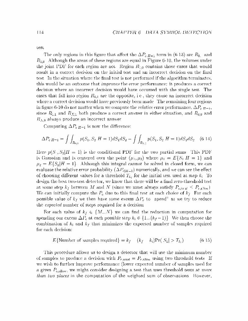
114 CHAPTER 6. DATA SYMBOL DETECTION

test.

The only regions in this �gure that a�ect the �PejH=1 term in (6.13) are R0;1 and

R1;0. Although the areas of these regions are equal in Figure 6-10, the volumes under

the joint PDF for each region are not. Region R1;0 contains those cases that would

result in a correct decision on the initial test and an incorrect decision on the �nal

test. In the situation where the �nal test is not performed if the algorithm terminates,

this would be an outcome that improves the error performance: it produces a correct

decision where an incorrect decision would have occurred with the single test. The

cases that fall into region R0;1 are the opposite, i.e., they cause an incorrect decision

where a correct decision would have previously been made. The remaining four regions

in �gure 6-10 do not matter when we compute the relative error performance, �PejH=1,

since R1;1 and RX;1 both produce a correct answer in either situation, and R0;0 and

RX;0 always produce an incorrect answer.

Computing �PejH=1 is now the di�erence:

�PejH=1 =Z Z

R0;1

p(S1; S2jH = 1)dS1dS2 �Z Z

R1;0

p(S1; S2jH = 1)dS1dS2 (6.14)

Here p(S1; S2jH = 1) is the conditional PDF for the two partial sums. This PDF

is Gaussian and is centered over the point (�1; �2) where �1 = EfS1jH = 1g and

�2 = EfS2jH = 1g. Although this integral cannot be solved in closed form, we can

evaluate the relative error probability (�PejH=1) numerically, and we can see the e�ect

of choosing di�erent values for a threshold Tki for the initial test used at step ki. To

design the best two-test detector, we know that there will be a �nal zero-threshold test

at some step kf between M and N (since we must always satisfy Pe;total � Pe;allow).

We can initially compute the Pe due to this �nal test at each choice of kf . For each

possible value of kf we then have some excess �Pe to \spend" as we try to reduce

the expected number of steps required for a decision.

For each value of kf 2 fM:::Ng we can �nd the reduction in computation for

spending our excess �Pe at each possible step ki 2 f1:::(kf�1)g. We then choose the

combination of ki and kf that minimizes the expected number of samples required

for each decision:

EfNumber of samples requiredg = kf � (kf � ki)Pr(jS1j > Tki) (6.15)

This procedure allows us to design a detector that will use the minimum number

of samples to produce a decision with Pe;total = Pe;allow using two threshold tests. If

we wish to further improve performance (lower expected number of samples used for

a given Pe;allow, we might consider designing a test that uses threshold tests at more

than two places in the computation of the weighted sum of observations. However,

6.4. DETECTION FOR CONTROLLED ERROR PROBABILITY 115

R0,0

R1,1RX,1

RX,0

R0,1

R1,0

S 1

1S >T

1

S 2

2S + S >0

Figure 6-10: Plot of the six di�erent regions for the di�erent combination of outcomes

of the two tests in the S1-S2 plane.

116 CHAPTER 6. DATA SYMBOL DETECTION

�nding the best combination of step number and thresholds for each step to minimize

the expected number of steps becomes more complex when more tests are used.

6.5 Performance of a two-test detector

Our goal in this �nal section is to quantify the potential performance gains are due

to some of the approaches to detection describe in previous sections. These gains due

to two speci�c e�ects which we will attempt to analyze separately. The �rst e�ect

is that of evaluating only the minimum number of samples necessary to achieve a

speci�c probability of error, as in Section 6.4.1.

This is seen by looking at the distribution of energy in a typical pulse, both for a

raised cosine pulse and a rectangular pulse with the same total energy for comparison

in Figure 6-11. Here we see the samples in sequential order in part (a), and also

the cumulative energy in the samples when sorted by decreasing magnitude in (b).

according to decreasing magnitude. We also see the cumulative energy (proportional

to amplitude squared) available in an evaluation of the sorted samples. Clearly many

samples are not useful to the receiver. In fact, this result shows that, in a sense, large

portions of the transmitted waveform are not useful in helping to communicate data

to receiver, although they are important for other reasons. Ons such function is in

shaping the spectrum of the transmitted signal, i.e., they help to reduce interference

seen by other receivers sharing the RF medium.

The implications of the energy distribution are seen in Figure 6-12, which shows

a plot of theoretical BER performance versus number of samples used for several

di�erent level of signal-to-noise ratio. In each case, it is clear that almost all of the

error performance is obtained from only a portion of the received samples.

These results illustrate how the idea of evaluating received samples in a greedy

manner enables us to reduce computation relative to a detector matched to the entire

pulse. In Figure 6-12 the computation could be reduced by almost a factor of 5�with little degradation in BER performance, or by more if higher BERs are tolerable.

In a sense, this greedy evaluation is equivalent to using the received sample in order

of decreasing SNR, which in this case would represent the ratio of signal energy to

noise energy in each sample.

The second e�ect that improves performance is the idea of using a second threshold

test to further reduce the average number of samples required for a decision with a

desired probability of error. A second test allows us to pick a non-zero threshold to

be used at some point prior to the �nal test. This threshold is chosen to balance the

e�ect of preventing some later incorrect decisions with the e�ect of inducing some

early additional errors. Performance is improved because any early decisions will

reduce the average number of samples used per decision. The threshold provides

6.5. PERFORMANCE OF A TWO-TEST DETECTOR 117

-0.2

0

0.2

0.4

0.6

0.8

1

-4 -3 -2 -1 0 1 2 3 4

Pul

se A

plitu

de

(a) Time

-0.2

0

0.2

0.4

0.6

0.8

1

-4 -3 -2 -1 0 1 2 3 4

Pul

se A

plitu

de

(a) Time

0

1

2

3

4

5

6

7

8

9

10

0 10 20 30 40 50 60 70 80 90 100

Cum

ulat

ive

Ene

rgy

in O

rder

ed S

ampl

es

(b) Proportion of Samples (%)

0

1

2

3

4

5

6

7

8

9

10

0 10 20 30 40 50 60 70 80 90 100

Cum

ulat

ive

Ene

rgy

in O

rder

ed S

ampl

es

(b) Proportion of Samples (%)

Figure 6-11: Plots of raised cosine and rectangular pulses (a) time domain and (b)

cumulative energy in sorted samples.

118 CHAPTER 6. DATA SYMBOL DETECTION

1e-14

1e-12

1e-10

1e-08

1e-06

0.0001

0.01

1

0 20 40 60 80 100

Bit

Err

or R

ate

Proportion of samples used for decision (%)

SNR=8

SNR=10

SNR=12

SNR=14

1e-14

1e-12

1e-10

1e-08

1e-06

0.0001

0.01

1

0 20 40 60 80 100

Bit

Err

or R

ate

Proportion of samples used for decision (%)

SNR=8

SNR=10

SNR=12

SNR=14

1e-14

1e-12

1e-10

1e-08

1e-06

0.0001

0.01

1

0 20 40 60 80 100

Bit

Err

or R

ate

Proportion of samples used for decision (%)

SNR=8

SNR=10

SNR=12

SNR=14

1e-14

1e-12

1e-10

1e-08

1e-06

0.0001

0.01

1

0 20 40 60 80 100

Bit

Err

or R

ate

Proportion of samples used for decision (%)

SNR=8

SNR=10

SNR=12

SNR=14

Figure 6-12: Plot of BER versus number of samples used in decision for various levels

of SNR.

a performance improvement by \spending" any excess error performance to reduce

computation at the expense of a carefully-controlled increase in BER up to the desired

maximum level.

The design of a two-test detector for speci�c set of performance speci�cations

proceeds in several steps. The two-test detector is designed for a speci�c level of

SNR and for a speci�c maximum probability of error. Given these two values, we

�rst �nd the step number for the �nal threshold test, kf . This is chosen as the

smallest number of samples that will always provide a error probability less than

the maximum allowable, Pe;kf � Pe;allow. Figure 6-13 shows the performance for a

detection scheme using only a �nal test at this lowest kf for a range of SNR values,

assuming that a minimum error probability is Pe;allow = 3� 10�3. The unusual shape

of the performance curve is due to the detection scheme using a di�erent number of

samples at di�erent SNR levels. The performance curve jumps between members of

a family of curves that would each be obtained using a �xed subset of the available

samples. A few of these curves are shown in Figure 6-13 as dashed lines for the

cases of decisions based on using only the largest one, two, or three samples. This

single-test scheme will ensure a satisfactory error probability, but does not yet provide

the lowest computation. In Figure 6-13, the data point marked with a star on the

modi�ed performance curve represents a BER of 2:3 � 10�3 at a SNR of 6 dB and

uses only seven of the 32 input samples. This BER is below the acceptable bound, so

we can further reduce the expected amount of computation by adding a second test

6.5. PERFORMANCE OF A TWO-TEST DETECTOR 119

1e-08

1e-07

1e-06

1e-05

0.0001

0.001

0.01

0.1

1

0 5 10 15 20

Bit

Err

or R

ate

SNR (dB)

Baseline Performance Performance with Minimum k_f

Allowable BER

1e-08

1e-07

1e-06

1e-05

0.0001

0.001

0.01

0.1

1

0 5 10 15 20

Bit

Err

or R

ate

SNR (dB)

Baseline Performance Performance with Minimum k_f

Allowable BER

1e-08

1e-07

1e-06

1e-05

0.0001

0.001

0.01

0.1

1

0 5 10 15 20

Bit

Err

or R

ate

SNR (dB)

Baseline Performance Performance with Minimum k_f

Allowable BER

1e-08

1e-07

1e-06

1e-05

0.0001

0.001

0.01

0.1

1

0 5 10 15 20

Bit

Err

or R

ate

SNR (dB)

Baseline Performance Performance with Minimum k_f

Allowable BER

1e-08

1e-07

1e-06

1e-05

0.0001

0.001

0.01

0.1

1

0 5 10 15 20

Bit

Err

or R

ate

SNR (dB)

Baseline Performance Performance with Minimum k_f

Allowable BER

1e-08

1e-07

1e-06

1e-05

0.0001

0.001

0.01

0.1

1

0 5 10 15 20

Bit

Err

or R

ate

SNR (dB)

Baseline Performance Performance with Minimum k_f

Allowable BER

1e-08

1e-07

1e-06

1e-05

0.0001

0.001

0.01

0.1

1

0 5 10 15 20

Bit

Err

or R

ate

SNR (dB)

Baseline Performance Performance with Minimum k_f

Allowable BER

1e-08

1e-07

1e-06

1e-05

0.0001

0.001

0.01

0.1

1

0 5 10 15 20

Bit

Err

or R

ate

SNR (dB)

Baseline Performance Performance with Minimum k_f

Allowable BER

Figure 6-13: Modi�ed performance curve for binary detection using minimum number

of samples to achieve bounded BER.

120 CHAPTER 6. DATA SYMBOL DETECTION

1

10

100

1000

10000

100000

1e+06

1 2 3 4 5 6

Thr

esho

ld R

equi

red

for

Spe

cifie

d M

axim

um B

ER

Step Number Where Initial Threshold Test is Performed

Figure 6-14: Lowest threshold value for potential values of ki.

at some step ki < kf that uses a non-zero threshold. This initial test will allow some

decisions to be made early to reduce the expected computation, while still ensuring

that the total error probability is below the allowable level.

Figure 6-14 shows the lowest threshold that can be used for each potential value of

ki < kf . This information is used to determine which value for ki will yield the lowest

expected amount of computation, which is shown in Figure 6-15. In the example

shown in the �gures, using an initial threshold test after the fourth data sample

reduces the expected amount of computation to about 5.3 samples per decision, a

reduction of about 25% below the result for the single, �xed test after the seventh

data sample.

There are several points to note in these results that would be interesting areas for

further work. The ability of this scheme to reduce computation depends on knowl-

edge of the current SNR conditions. This is not unreasonable for a wireless system;

many current wide area wireless networks periodically transmit sequences of known

data to enable the receiver to estimate channel conditions [Rappaport, 1996]. The

e�ect of uncertainly in the SNR estimate has not been analyzed in this work, but

would be important factor in an actual implementation. Equally important would be

6.5. PERFORMANCE OF A TWO-TEST DETECTOR 121

5

5.5

6

6.5

7

7.5

8

1 2 3 4 5 6

Exp

ecte

d N

umbe

r of

Ste

ps R

equi

red

Step Number Where Initial Threshold Test is Performed

Figure 6-15: Expected number of samples required for each bit decision using a two-

test detector.

122 CHAPTER 6. DATA SYMBOL DETECTION

the scheme's performance under dynamic SNR conditions. This technique could be

modi�ed to use tests at di�erent times and di�erent threshold values in response to

changes in SNR. This would add complexity to the implementation, but the potential

savings in computation might be worth it.

6.6 Summary

This chapter describes an approach to data symbol detection that allows a wireless re-

ceiver to reduce computational complexity by computing decisions with a sub-optimal,

but bounded, BER. The results show two e�ective techniques for reducing computa-

tion. The �rst technique is to approximate the optimal decision by using a partial

evaluation of the matched �lter sum. We showed that the best way to approximate

the sum is to use evaluate the received samples using a greedy ordering according to

the magnitude of the corresponding �lter coe�cients. We can compute how many

samples should be evaluated in the partial sum as a function of the desired BER and

the current SNR.

The second technique is used to further reduce computation by introducing a

second threshold test after only a portion of the approximate sum has been evaluated.

This initial test can be designed to allow some of the decisions to be made early while

ensuring that the acceptable level of BER is achieved. This second technique results

in a run-time that is statistical, but which is lower than the original run-time that

was achievable using a deterministic decision rule.

Chapter 7

Summary, Contributions and

Future Work

In this thesis, we presented the results of an investigation of how physical layer pro-

cessing algorithms can balance exibility and e�ciency in wireless communication

systems. The work was motivated by a number of trends that are changing the type

of service expected from wireless communications systems of the future. These trends

include more dynamic environmental conditions, heterogeneous tra�c, and increasing

demands for e�ciency and performance. All of these trends have implications on the

physical layer implementation of the communication system.

Given these trends, we believe that it will be di�cult, if not impossible, to design

a static physical layer that will be able to provide e�cient service in all of the di�erent

anticipated situations. This led us to investigate the design of DSP algorithms that

provide processing that is both exible and computationally e�cient.

As we began to develop algorithms that could balance exibility and e�ciency,

it became clear that we needed a precise understanding about the speci�c types of

exibility that would be useful in each situation. In other words, we needed an im-

proved understanding of how a system could be designed to exploit better conditions:

e.g., how could it exploit better SNR conditions to lower processing requirements?

In a number of cases addressed in this thesis, the answer to this question was that

we could specify the requirements for processing in speci�c portions of the system so

that in better conditions we could produce a su�ciently high quality result using less

computation.

Furthermore, we began to understand that producing DSP algorithms to e�ciently

compute approximate results requires, in many cases, a more careful understanding of

the speci�c relationship between input and output samples for the signal processing

function in question.

In this thesis, this idea has been articulated through the concept of sub-sampling

123

124 CHAPTER 7. SUMMARY, CONTRIBUTIONS AND FUTURE WORK

and the idea of the footprint of a desired result. The random sub-sampling techniques

described in Chapter 5 recognize that an approximate result for a frequency selective

�lter needs to be computed from data that span the same interval of time, but need

only use a subset of those samples in that interval. Similarly, the idea of a symbol

footprint in Chapter 6 stems from the need to identify the precise set of samples that

had information relevant to a speci�c symbol estimate in a detector. In this case, an

approximate result can be found using a subset of the samples in the footprint. This

led to an investigation of which samples in the footprint were most useful and would

therefore be used �rst.

In other situations, approximate results are not appropriate. In these cases, how-

ever, the same understanding of input-output data relationships led to algorithms

that could produce the desired results using less computation by taking advantage of

larger amounts of memory or removing intermediate processing steps.

In all of these cases, it was also important to understand the role of each processing

stage within the large communications system. It is this understanding that led to

the conclusion that approximate results would be su�cient in some cases, or that

intermediate processing stages could be eliminated because they were unnecessary

for overall system operation.

One �nal aspect of this work that has been instrumental in helping to guide the

choice of problems and validate the results has been the implementation of the algo-

rithms in a working wireless communications system. Some of these implementations

were described in chapters 4 and 5 of this thesis. These implementation e�orts helped

to identify important issues for the design of new signal processing algorithms, such as

the relative costs of memory access and computation, and have also led us to identify

new areas for future investigation.

7.1 Contributions

This thesis has demonstrated that it is possible to design DSP algorithms for the

physical layer of a wireless communications system that is itself designed to use ex-

ibility to improve overall system performance. These algorithms allow the system

to take advantage of variable conditions in the wireless channel and changing sys-

tem performance requirements to provide more e�cient system operation. In this

algorithm development work, we have achieved the following:

� Developed an E�cient Digital Modulation Technique: Direct waveform

synthesis is a technique that e�ciently synthesizes digitally modulated wave-

forms at IF. This technique provides a 20�25� computation reduction relative

to conventional techniques using a look-up table of pre-computed samples. We

7.1. CONTRIBUTIONS 125

also described table decomposition techniques that allow a exible trade-o�

between memory and computation required to synthesize di�erent waveforms.

� Separated Bandwidth Reduction from SNR Control in FIR Filters:

Conventional FIR �lter design techniques assume that �lters will operate on

contiguous blocks of input samples. This assumption leads to an unnecessarily

coupling between the length of the FIR �lter and the number of input samples

used. We have demonstrated a model for �ltering that decouples the require-

ment for a long �lter response from the number of input samples used, avoiding

excessive computation. This decoupling is accomplished through algorithms

that use only as many input samples as necessary to compute output signals

with the desired SNR levels.

� Developed a Frequency-Translating Filter: Our technique shows how the

function of arbitrary frequency translation can be combined with a decimating

FIR �lter through the design of a composite �lter followed by a frequency shift

at the lower output sample rate. We also described how the use of a complex-

valued �lter design can lead to an additional two-fold reduction in computation

by reducing the number of coe�cients required for the �lter.

� Demonstrated the E�ectiveness of Random Sub-sampling: This tech-

nique is used to realize the decoupling of bandwidth reduction and SNR control

in the channel separation �lter. Random sub-sampling provides an e�ective way

to approximate the input sample stream of a narrowband FIR �lter, allowing

us to control the trade-o� between computation and output SNR.

Using the analytical model we developed to understand this technique, we

showed that amount of computation required to produce an output signal with

desired SNR depends only on the output sample rate and the signal energy in

the �lter stopband, not on the �lter input sample rate. This result allows us

to increase the input bandwidth of the system without increasing the compu-

tation required to separate each channel or, conversely, to narrow the output

bandwidth and reduce the required computation accordingly.

� Designed a Detector that Provides Controlled Error Probability: We

demonstrate how to design a matched �lter detector that uses multiple thresh-

old tests to provide signi�cant computational saving relative to a conventional

implementation. The reduction in computation is due to two distinct e�ects.

First, we demonstrate that widely-used pulse shaping techniques result in a

concentration of the useful signal energy in a small number of samples. Our

technique identi�es those most useful samples, providing a reduction in com-

putation of �ve-fold or more relative to evaluating the full matched �lter sum.

126 CHAPTER 7. SUMMARY, CONTRIBUTIONS AND FUTURE WORK

Secondly, we introduce an additional threshold test early in the computation.

The timing and threshold value for this test are chosen to minimize computation

while ensuring the desired error probability for symbol decisions.

7.2 Future Work

Each of the accomplishments above demonstrate that understanding the role of the

DSP algorithms in the context of the larger system can lead to signi�cant perfor-

mance gains. Future systems will experience more situations where dynamic channel

conditions and changing application needs will call for a exible physical layer design

to more e�ectively provide the communications services desired by the endpoint users.

7.2.1 Investigation of Additional Physical Layer Functions

There are a number of other functions required in the physical layer of some wire-

less systems that were not investigated in this work. The synchronization functions

required in a digital receiver are critical to e�ective symbol detection and, like detec-

tion, their complexity can vary heavily depending on the signal conditions and the

demands of the systems. Flexible techniques to provide synchronization functions,

such as symbol timing recovery, could lead to more e�cient implementations and

better performance.

Also, the trend toward higher data-rate systems will lead to a greater need for

e�ective equalization techniques to compensate for multipath interference. Equaliza-

tion often requires intensive processing and depends heavily on the conditions in the

wireless channel. A exible approach to equalization could lead to signi�cant gains

when favorable conditions allow a reduction in processing.

7.2.2 Flexible System Design

This work involved the design of DSP algorithms that exhibit speci�c modes of ex-

ibility in their behavior. These types of behavior were chosen to allow the overall

system to bene�t from changing conditions or performance requirements. Many of

the improvements suggested in this work, however, allow a single stage of processing

to improve its e�ciency using information about the overall system requirements. An

important area of study is how to coordinate exible behavior changes amongmultiple

components of a system to improve performance. Work in [Secor, 1996] investigates

how to coordinate networks of processing stages to e�ciently accomplish system pro-

cessing goals. The use of such techniques in a wireless communications system could

lead to further improvements in system performance under changing conditions.

7.3. CONCLUSIONS 127

7.3 Conclusions

The dynamic nature of the wireless operating environment and the variable perfor-

mance requirements of wireless applications is in con ict with the traditional static

implementations of the physical layer. The dynamic channel and variable performance

requirements preclude e�ective static optimization of the physical layer processing,

and provide an opportunity for exible implementations to dramatically improve over-

all system performance. This presents an opportunity for exible algorithms that can

enable the entire communication system to adapt to the changing conditions and de-

mands. We believe that future wireless systems will have to incorporate this type of

physical layer exibility if they are to provide the types of e�cient communications

services expected by the users of tomorrow.

It is often assumed that exibility in an algorithm comes at the cost of reduced

computational e�ciency. In this thesis, however, we have demonstrated a suite of

exible algorithms that take advantage of changing conditions and system demands

to provide signi�cantly improved performance relative to static designs.

Although the results of this work are very encouraging, we believe that the al-

gorithms presented are just a start, and that there are still many signi�cant and

interesting problems to be solved. Complex system requirements and technological

advances have led to a merging of the �elds of digital signal processing, theoreti-

cal computer science and communications system design. We believe that e�ective

designs for the systems of tomorrow will need to draw on results from all of these

disciplines to meet the growing demand for communication services without wires.

128 CHAPTER 7. SUMMARY, CONTRIBUTIONS AND FUTURE WORK

Bibliography

[Baines, 1995] Baines, R. (1995). The DSP Bottleneck. IEEE Communications Mag-

azine, 33(5):46{54.

[Berlecamp et al., 1987] Berlecamp, E., Peile, R., and Pope, S. (1987). The applica-

tion of error controls to communicatitons. IEEE Communiations Magazine.

[Bilinskis and Mikelsons, 1992] Bilinskis, I. and Mikelsons, A. (1992). Randomized

Signal Processing. Prentice Hall.

[Bose, 1999] Bose, V. (1999). Design and Implementation of Software Radios using

a General Purpose Processor. PhD thesis, Massachusetts Institute of Technology.

[Bose et al., 1999] Bose, V., Ismert, M., Welborn, M., and Guttag, J. (1999). Virtual

Radios. IEEE JSAC issue on Software Radios.

[Cover and Thomas, 1990] Cover, T. and Thomas, J. (1990). Elements of Informa-

tion Theory. John Wiley and Sons.

[Crochiere and Rabiner, 1981] Crochiere, R. and Rabiner, L. (1981). Interpolation

and decimation of digital signals: a tutorial review. Proceedings of the IEEE.

[Frerking, 1994] Frerking, M. E. (1994). Digital Signal Processing in Communiations

Systems. Van Nostrand Reinhold.

[Frigo and Johnson, 1997] Frigo, M. and Johnson, S. (1997). The fastest fourier trans-

form in the west. Technical Report MIT-LCS-TR-728, MIT Laboratory for Com-

puter Science.

[Grant et al., 2000] Grant, D., Randers, E., and Zvonar, Z. (2000). Data over cellular:

A look at GPRS. Communications System Design.

[Hogenauer, 1981] Hogenauer, E. (1981). An economical class of digital �lters for

decimation and interpolation. IEEE Transactions on Acoustics, Speech and Signal

Processing.

129

130 BIBLIOGRAPHY

[Ismert, 1998] Ismert, M. (1998). Making Commodity PCs Fit for Signal Processing.

In USENIX. USENIX.

[J. C. Liberti and Rappaport, 1999] J. C. Liberti, J. and Rappaport, T. S. (1999).

Smart Antennas for Wireless Communications: IS-95 and Third Generation

CDMA Applications. Prentice Hall.

[Jackson, 1989] Jackson, L. B. (1989). Digital Filters and Signal Processing. Kluwar

Academic Publishers.

[Komodromos et al., 1995] Komodromos, M., Russell, S., and Tang, P. T. P. (1995).

Design of FIR �lters with complex desired frequency response using a generalize re-

mez algorithm. IEEE Transactions on Circuits and Systems II: Analog and Digital

Signal Processing.

[Lee and Messerschmitt, 1994] Lee, E. A. and Messerschmitt, D. G. (1994). Digital

Communication. Kluwer Academic Publishers, 2nd edition.

[Lorch and Smith, 1998] Lorch, J. and Smith, A. (1998). Software strateies for

portable computer energy management. IEEE Personal Communications.

[Ludwig, 1997] Ludwig, J. (1997). Low power digital �ltering using adaptive process-

ing processing. PhD thesis, Massachusetts Institute of Technology.

[Meyr et al., 1997] Meyr, H., Moeneclay, M., and Fechtel, S. A. (1997). Digital Com-

munication Receivers: Synchronization, Channel Estimation, and Signal Process-

ing. John Wiley and Sons.

[Mitola, 1995] Mitola, J. (1995). The Software Radio Architecture. IEEE Commu-

nications Magazine, 33(5):26{38.

[Nawab et al., 1997] Nawab, S. H., Oppenheim, A. V., Chandrakasan, A. P., Wino-

grad, J. M., and Ludwig, J. T. (1997). Approximate signal processing. J. VLSI

Sig. Proc.

[Ochi and Kambayashi, 1988] Ochi, H. and Kambayashi, N. (1988). Design of com-

plex coe�cient FIR digital �lters using weighted approximation. In Proceeding of

ISCAS.

[Oppenheim and Schafer, 1989] Oppenheim, A. V. and Schafer, R. W. (1989).

Discrete-Time Signal Processing. Prentice Hall.

[Orfanidis, 1996] Orfanidis, S. (1996). Introduction to Signal Processing. Prentice-

Hall.

BIBLIOGRAPHY 131

[Proakis, 1995] Proakis, J. G. (1995). Digital Communications. McGraw Hill.

[Rao, 2000] Rao, S. (2000). Architecture for abaptible wirelesss networks. Master's

thesis, Massachusetts Institute of Technology.

[Rappaport, 1991] Rappaport, T. (1991). The wireless revolution. IEEE Communi-

ations Magazine.

[Rappaport, 1996] Rappaport, T. S. (1996). Wireless Communications: Principles

and Practice. Prentice Hall.

[Reed, 1998] Reed, J. H. (1998). Direct digital synthesis. In Tutorial notes from

PMIRC 1998.

[Saltzer et al., 1981] Saltzer, J. H., Reed, D. P., and Clark, D. D. (1981). End-to-end

arguments in system design. In Second International Conference on Distributed

Computing Systems.

[Secor, 1996] Secor, M. (1996). Modelling and optimizing quality for networks of

approximate processors. Master's thesis, Massachusetts Institute of Technology.

[Stallings, 1990] Stallings, W. (1990). Handbook of Computer-Communications stan-

dards, Vol. 2. Stallings/MacMillan.

[Stark and Woods, 1986] Stark, H. and Woods, J. (1986). Probability, Random

Porcesses, and Estimation Theory for Engineers. Prentice-Hall, Inc.

[Steiglitz et al., 1992] Steiglitz, K., Parks, T. W., and Kaiser, J. F. (1992). METEOR:

A constraint-based FIR �lter design program. IEEE Transactions on Signal Pro-

cessing.

[Stemm and Katz, 1997] Stemm, M. and Katz, R. (1997). Measuring and reducing

energy consumptio of network interfaces in hand-held devices. IEICE Transactions

on Fundamentals of Electronics, Communications, and Computer Science, Special

Issue on Mobile Computing.

[Vasconcellos, 1999] Vasconcellos, B. (1999). Parallel signal processing for everyone.

Master's thesis, Massachusetts Institute of Technology.

[Welborn, 1999] Welborn, M. (1999). Direct waveform synthesis for software radios.

In Proceedings of WCNC.

[Wepman, 1995] Wepman, J. A. (1995). Analog-to-Digital Convertors and Their Ap-

plications in Radio Receivers. IEEE Communications Magazine, 33(5):39{45.

132 BIBLIOGRAPHY

[Wicker, 1995] Wicker, S. (1995). Error Control Systems for Digital Communications

and Storage. Prentice Hall.

[Wiesler and Jondral, 1998] Wiesler, A. and Jondral, F. (1998). Software radio struc-

ture for second generation mobile communication systems. In Proceedings of VTC.

[Winograd, 1997] Winograd, J. M. (1997). Incremental re�nement structures for ap-

proximate signal processing. PhD thesis, Boston University.

[Winograd et al., 1996] Winograd, J. M., Nawab, J. T. L. S. H., Oppenheim, A. V.,

and Chandrakasan, A. P. (1996). Flexible systems for digital signal processing. In

AAAI Fall Symposium on Flexible Computation.

[Zangi and Koilpillai, 1999] Zangi, K. and Koilpillai, R. D. (1999). Software radio

issues in cellular basestations. IEEE JSAC issue on Software Radios.

[Zilberstein, 1993] Zilberstein, S. (1993). Operational Rationality through Compila-

tion of Anytime Algorithms. PhD thesis, Computer Science Division, University of

California at Berkeley.

[Zilberstein, 1996] Zilberstein, S. (1996). Optimal composition of real-time systems.

Arti�cial Intelligence.