flexible regression and smoothing - tu graz · zero adjusted ga y pdf l ... pepower exponential (1...

Flexible Regression and SmoothingThe gamlss.family Distributions

Bob Rigby Mikis Stasinopoulos

Graz University of Technology, Austria, November 2016

Bob Rigby, Mikis Stasinopoulos Flexible Regression and Smoothing 2013 1 / 41

Outline

1 Types of distribution in GAMLSS

2 Continuous distributionsTypes of continuous distributionsSummary of methods of generating distributionsTheoretical ComparisonTypes of tailsFitting a distribution

3 End


Outline

Information


Types of distribution in GAMLSS

Different types of distribution

1 continuous distributions: fY (y |θ), are usually defined on (−∞,+∞),(0,+∞) or (0, 1).

2 discrete distributions: P(Y = y |θ) are defined on y = 0, 1, 2, . . . , n,where n is a known finite value or n is infinite, i.e. usually discrete(count) values.

3 mixed distributions: (finite mixture distributions) are mixtures ofcontinuous and discrete distributions, i.e. continuous distributionswhere the range of Y has been expanded to include some discretevalues with non-zero probabilities.



Different types of distribution: demos

1 demo.GA()

2 demo.PO()

3 demo.BI()

4 demo.BE()

5 demo.BEINF()



Example of continuous distribution: SEP1

−4 −2 0 2 4

0.00.4

0.81.2

(a)

y

f(y)

−4 −2 0 2 4

0.00.2

0.40.6

0.8

(b)

y

f(y)

−4 −2 0 2 4

0.00.2

0.40.6

(c)

y

f(y)

−4 −2 0 2 4

0.00.2

0.40.6

0.81.0

(d)

y

f(y)



Example of discrete distribution: Sichel

0 5 10 15 20

0.00

0.05

0.10

0.15

Sichel, SICHEL

SICHEL( mu = 5, sigma = 11.04, nu = 0.98 )

y

pf, f(y

)

0 5 10 15 20

0.00

0.05

0.10

0.15

Sichel, SICHEL

SICHEL( mu = 5, sigma = 1.151, nu = 0 )

y

pf, f(y

)

0 5 10 15 20

0.00

0.05

0.10

0.15

Sichel, SICHEL

SICHEL( mu = 5, sigma = 0.9602, nu = −1 )

y

pf, f(y

)

0 5 10 15 20

0.00

0.05

0.10

0.15

Sichel, SICHEL

SICHEL( mu = 5, sigma = 43.9, nu = −3 )

y

pf, f(y

)



Example of mixed distribution distributions: ZAGA

0 2 4 6 8 10

0.00

0.05

0.10

0.15

Zero adjusted GA

y

pdf ●

0 5 10 15 20

0.00.4

0.8

Zero adjusted Gamma c.d.f.

y

F(y)

●


Continuous distributions Types of continuous distributions

Types of continuous distributions

0 5 10 15 20

0.00

0.05

0.10

0.15

negative skewness

y

f(y)

0 5 10 15 20 25 30

0.00

0.05

0.10

0.15

positive skewness

y

f(y)

0 5 10 15 20

0.00

0.04

0.08

platy−kurtosis

y

f(y)

0 5 10 15 200.0

00.1

00.2

0

lepto−kurtosis

y

f(y)

Figure: Showing different types of continuous distributions



Two parameter continuous distributions in GAMLSS

Two parameter distributions

BE Beta (0, 1)

GA Gamma (0,∞)

GU Gumbel (−∞,∞)

LO Logistic (−∞,∞)

LNO Log Normal (0,∞)

NO Normal (−∞,∞)

IG Inverse Gaussian (0,∞)

RG Reverse Gumbel (−∞,∞)

WEI Weibull (also WEI2, WEI3) (0,∞)



Three parameter continuous distributions in GAMLSS

Three parameter distributions

BCCG Box-Cox Normal (0,∞)

exGAUS Exponential-Gaussian (−∞,∞)

GG Generalized Gamma (0,∞)

GIG Generalized Inverse Gaussian (0,∞)

PE Power Exponential (−∞,∞)

TF t family (−∞,∞)

SN1 skew normal type 1 (−∞,∞)

SN2 skew normal type 2 (−∞,∞)



Two and three parameters comparison: demos

1 demo.PE.NO()

2 demo.TF.NO()



Four parameter continuous distributions in GAMLSS

Four parameter distributions

BCT Box-Cox t (0,∞)

BCPE Box-Cox Power Exponential (0,∞)

EGB2 Exponential Generalized Beta type 2 (−∞,∞)

GT Generalized t (−∞,∞)

JSU Johnson Su (−∞,∞)

SHASH Sinh Arc-Sinh (−∞,∞)

SEP1-SEP4 Skew Exponential Power (−∞,∞)

ST1-ST5 Skew t (−∞,∞)

SST Shew t (−∞,∞) repar. of ST3



Continuous GAMLSS family distributions defined on(−∞,+∞)

Distributions family no par. skewness kurtosis

Exp. Gaussian exGAUS 3 positive -

Exp.G. beta 2 EGB2 4 both lepto

Gen. t GT 4 (symmetric) lepto

Gumbel GU 2 (negative) -

Johnson’s SU JSU, JSUo 4 both lepto

Logistic LO 2 (symmetric) (lepto)

Normal-Expon.-t NET 2,(2) (symmetric) lepto

Normal NO-NO2 2 (symmetric)

Normal Family NOF 3 (symmetric) (meso)



Continuous GAMLSS family distributions defined on(−∞,+∞)

Power Expon. PE-PE2 3 (symmetric) both

Reverse Gumbel RG 2 positive

Sinh Arcsinh SHASH, 4 both both

Skew Exp. Power SEP1-SEP4 4 both both

Skew t ST1-ST5, SST 4 both lepto

t Family TF 3 (symmetric) lepto



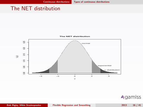
The NET distribution

−4 −2 0 2 4

0.000.05

0.100.15

0.200.25

Y

f Y(y)

The NET distribution

normal

exponential

t−distribution



Continuous GAMLSS family distributions defined on(0,+∞)


BCCG BCCG 3 both

BCPE BCPE 4 both both

BCT BCT 4 both lepto

Exponential EXP 1 (positive) -

Gamma GA 2 (positive) -

Gen. Beta type 2 GB2 4 both both

Gen. Gamma GG-GG2 3 positive -

Gen. Inv. Gaussian GIG 3 positive -

Inv. Gaussian IG 2 (positive) -

Log Normal LOGNO 2 (positive) -

Log Normal family LNO 2,(1) positive

Reverse Gen. Extreme RGE 3 positive -

Weibull WEI-WEI3 2 (positive) -



Positive response: Transformation from (−∞,∞) to(0,+∞)

Any distribution for Z on (−∞,∞) can be transformed to acorresponding distribution for Y = exp(Z ) on (0,+∞)

For example: from t distribution to log t distribution

gen.Family("TF", type="log")



Positive response: log T distribution

0 2 4 6 8 10

0.00.2

0.40.6

x

dlogTF(

x, mu =

0)

0 2 4 6 8 10

0.00.2

0.40.6

0.81.0

x

plogTF(

x, mu =

0)

0.0 0.2 0.4 0.6 0.8 1.0

05

1015

x

qlogTF(

x, mu =

0)

Histogram of Y

Y

Frequen

cy

0 5 10 15 20 25 30

050

100150



Positive response: demos

1 demo.NO.LOGNO()

2 demo.BCPE()



Continuous GAMLSS family distributions defined on(0, 1)


Beta BE 2 (both) -

Beta original BEo 2 (both) -

Logit normal LOGITNO 2 (both) -

Generalized beta type 1 GB1 4 (both) (both)



Continuous GAMLSS family distributions defined on(0, 1): Transformation from (−∞,∞) to (0, 1)

Any distribution for Z on (−∞,∞) can be transformed to acorresponding distribution for Y = 1

1+e−Z on (0, 1)

For example: from t distribution to logit t distribution

gen.Family("TF", "logit")



Continuous GAMLSS family distributions defined on(0, 1): logit T distribution

0.0 0.2 0.4 0.6 0.8 1.0

0.51.0

1.5

x

dlogitTF

(x, mu =

0)

0.0 0.2 0.4 0.6 0.8 1.0

0.00.2

0.40.6

0.81.0

x

plogitTF

(x, mu =

0)

0.0 0.2 0.4 0.6 0.8 1.0

0.00.2

0.40.6

0.81.0

x

qlogitTF

(x, mu =

0)

Histogram of Y

Y

Frequen

cy

0.0 0.2 0.4 0.6 0.8 1.0

05

1015

2025

30



Four parameters from 0 to 1: demos

1 demo.GB1()


Continuous distributions Summary of methods of generating distributions

Summary of methods of generating distributions

1 univariate transformation from a single random variable (LOGNO,BCCG, BCPE, BCT, EGB2, SHASHo, inverse log and logictransformations . . .)

2 transformation from two or more random variables (TF, ST2,exGAUS)

3 truncation distributions

4 a (continuous or finite) mixture of distributions (TF, GT, GB2, EGB2)

5 Azzalini type methods (SN1, SEP1, SEP2, ST1, ST2)

6 splicing distributions (SN2, SEP3, SEP4, ST3, ST4, NET)

7 stopped sums

8 systems of distributions


Continuous distributions Theoretical Comparison

Comparison of properties of distributions

1 Explicit pdf cdf and inverse cdf

2 Explicit centiles and centile based measures (e.g median)

3 Explicit moment based measures (e.g. mean)

4 Explicit mode(s)

5 Continuity of the pdf and its derivatives with respect to y

6 Continuity of the pdf with respect to µ, σ, ν and τ

7 Flexibility in modelling skewness and kurtosis

8 Range of Y



Theoretical comparison of distributions

OK we have a lot of distributions in GAMLSS.Do we need any more?

Do we need all of them or some of them are redundant?

Is there any way to compare them theoretically?

We can compare the tail behaviour in of the distributions

Since most of then are location-scale we can compare their flexibilityin terms of skewness and kurtosis



Comparing tails: real line

−10 −5 0 5 10

−12−10

−8−6

−4−2

x

log(pdf)

NormalCauchyLaplace



Comparing tails: positive real line

0 5 10 15 20 25 30

−7−6

−5−4

−3−2

−10

x

log(pdf)

exponentialPareto 2log Normal


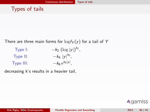
Continuous distributions Types of tails

Types of tails

There are three main forms for logfY (y) for a tail of Y

Type I: −k2 (log |y |)k1 ,

Type II: −k4 |y |k3 ,

Type III: −k6 ek5|y |,

decreasing k’s results in a heavier tail,



Types of tails: classification (real line)



Types of tails: classification (positive real line)


Continuous distributions Fitting a distribution

How to fit distributions in R

optim() or mle() requires initial parameter values

gamlsssML() mle a using variation of the mle() function

gamlss(): mle using RS or CG or mixed algorithms,

histdist() mle using RS or CG or mixed algorithms, for a univariatesample only, and plots a histogram of the data with thefitted distribution

fitDist() fits a set of distributions and chooses the one with thesmallest GAIC



Strength of glass fibres data

Data summary:

R data file: glass in package gamlss.data of dimensions 63× 1

sourse: Smith and Naylor (1987)

strength: the strength of glass fibres (the unitof measurement are not given).

purpose: to demonstrate the fitting of a parametricdistribution to the data.

conclusion: a SEP4 distribution fits adequately



Strength of glass fibres data: SBC

glass strength

glass$strength

Frequenc

y

0.5 1.0 1.5 2.0

05

1015

20



Strength of glass fibres data: creating truncateddistribution

data(glass)

library(gamlss.tr)

gen.trun(par = 0, family = TF)

A truncated family of distributions from TF

has been generated

and saved under the names:

dTFtr pTFtr qTFtr rTFtr TFtr

The type of truncation is left and the

truncation parameter is 0



Strength of glass fibres data: fitting the models

> m1<-fitDist(strength, data=glass, k=2, extra="TFtr")

# AIC

> m2<-fitDist(strength, data=glass, k=log(length(strength)),

extra="TFtr") # SBC

> m1$fit[1:8]

SEP4 SEP3 SHASHo EGB2 JSU BCPEo ST2 BCTo

27.68790 27.98191 28.01800 28.38691 30.41380 31.17693 31.40101 31.47677

> m2$fit[1:8]

SEP4 SEP3 SHASHo EGB2 GU WEI3 JSU PE

36.26044 36.55444 36.59054 36.95945 38.19839 38.69995 38.98634 39.00792



Strength of glass fibres data: Results

histDist(glass$strength, SEP4, nbins = 13,

main = "SEP4 distribution",

method = mixed(20, 50))



Strength of glass fibres data: SBC

0.5 1.0 1.5 2.0 2.5

0.00.5

1.01.5

2.02.5

SEP4 distribution

glass$strength

f()



Strength of glass fibres data: summary

Call: gamlss(formula = y~1, family = FA)

Mu Coefficients:

(Intercept)

1.581

Sigma Coefficients:

(Intercept)

-1.437

Nu Coefficients:

(Intercept)

-0.1280

Tau Coefficients:

(Intercept)

0.3183

Degrees of Freedom for the fit: 4 Residual Deg. of Freedom 59

Global Deviance: 19.8111

AIC: 27.8111

SBC: 36.3836Bob Rigby, Mikis Stasinopoulos Flexible Regression and Smoothing 2013 40 / 41

End

ENDfor more information see

www.gamlss.org


flexible regression and smoothing - tu graz · zero adjusted ga y pdf l ... pepower exponential (1...

Documents