TECHNICAL NOTE 73298

Flexible HPLC instrument setups for double usage as one heart-cut-2D-LC system or two independent 1D-LC systems

Authors: Maria Grübner and Giorgia Greco

Thermo Fisher Scientific, Germering, Germany

Keywords: Two-dimensional liquid chromatography, 2D-LC, 2D-HPLC, heart-cut-2D-LC, Vanquish Duo UHPLC System, Vanquish Dual Split Sampler, Chromeleon, SII for Xcalibur, SII for Empower

GoalShowcase several heart-cut 2D-LC setups with elution strength reduction implemented with the Thermo Scientific™ Vanquish™ UHPLC platform and highlight the benefit of the Thermo Scientific™ Vanquish™ Dual Split Sampler to build a flexible system, which can be used either as one heart-cut 2D-LC system or as two independent 1D-LC systems

Benefits• Heart-cut 2D-LC with analyte trapping during fraction

transfer enables straightforward peak identity and purity confirmation by MS detection despite MS incompatible mobile phases in the first-dimension separation.

• The Vanquish Dual Split Sampler in a 2D-LC setup greatly improves the instrument usability and value.

• Flexible, software-aided switching between the application options as a heart-cut 2D-LC system or as two independent 1D-LC systems enables more efficient instrument operation and increases the return on investment of the LC instrument as well as of associated MS detectors.

IntroductionConventional liquid chromatography (LC) separations are referred as one-dimensional (1D) as the sample is subjected to one single separation process. However,

2

despite considerable improvements in the commercially available LC hardware (instrumentation as well as column technology), 1D-LC sometimes cannot meet the demands in separation and resolution capabilities of the analytical task.1,2 Sometimes a sufficient solution is the analysis of one sample by dual or multiple complementary techniques.3 Another recent trend goes towards two-dimensional (2D) LC techniques, meaning in general that fractions eluting from the first dimension (1D) are further analyzed by a second dimension (2D) separation. Herein, the selection of orthogonal dimensions increases the available separation space and thus the probability to resolve the compounds of interest.2 The interface connecting both dimensions usually consists of a combination of fluidic valves and storage loops or trap columns. Such setups are referred to as online 2D-LC as the transferred fractions do not leave the fluidic system. There are also offline 2D-LC setups, where fractions from the 1D are collected externally into vials for a later reinjection into the 2D.2,4 The technique heart-cut 2D-LC refers to the transfer of a single fraction; multi-heart-cut 2D-LC refers to the transfer of several fractions; and comprehensive 2D-LC refers to the transfer of the whole 1D eluate in a large number of fractions.4 Comprehensive 2D-LC is a powerful tool in achieving separation of highly complex samples with 100–1000 components as it is needed, for example, in omics research areas.

However, comprehensive 2D-LC also often overshoots the actual analytical task, when only one or a few fractions are of greater interest. For example, one frequently requested application relates to the unambiguous identification and purity confirmation of single peaks in quality control (QC) labs. Commonly utilized phosphate and other mass spectrometry (MS) incompatible buffers in the mobile phase of LC-UV methods usually prevent their direct transfer to MS detection. Thus, if further confirmation by MS is needed, an adjustment of the 1D-LC method is required, such as the use of MS compatible eluent additives. Resulting differences in the elution pattern compared to the original method cause extra effort and documentation for justification, especially in a regulated environment. A preferred solution in such cases is a direct transfer of the respective peak (heart-cut) from the 1D LC-UV run to an MS compatible 2D LC-MS separation, preferably

combined with a desalting step for the removal of residual salts from the 1D mobile phase.5 The current technical note summarizes several possibilities to set up heart-cut 2D-LC systems implemented with the Thermo Scientific™ Vanquish™ UHPLC platform, provides strengths of each setup, and highlights the benefit of employing the Thermo Scientific™ Vanquish™ Dual Split Sampler to create a flexible system, which can be used either as one heart-cut 2D-LC system or as two independent 1D-LC systems. Software method setup is illustrated as well.

Experimental Chemicals• Deionized water, 18.2 MΩ·cm resistivity or higher

• Fisher Scientific™ Acetonitrile, Optima™ LC/MS grade (P/N A955-212)

• Fisher Scientific™ Methanol, Optima™ LC/MS grade (P/N A456-212)

• Fisher Scientific™ Formic acid, Optima™ LC/MS grade (P/N A117-50)

• Fisher Chemical™ ortho-Phosphoric acid (85%) (P/N O/0515/PB08)

• Desmedipham and Phenmedipham were provided by a reputable vendor

Sample handling• Vials (amber, 1.5 mL) (P/N 6000.0072)

• Thermo Scientific™ SUN-SRi 11 mm Orange Snap Caps PTFE/Sil (P/N 501 382)

Instrumentation• Thermo Scientific™ Vanquish™ Flex UHPLC system

consisting of:

– Vanquish System Base (P/N VF-S01-A-02)

– Vanquish Quaternary Pump F (P/N VF-P20-A-01) [for 1D]

– Vanquish Binary Pump F (P/N VF-P10-A-01) [for 2D]

3

– Vanquish Split Sampler FT (P/N VF-A10-A-02)

– or Vanquish Dual Split Sampler FT (P/N VF-A40-A-01)

– 1× or 2× Vanquish Column Compartment H (P/N VH-C10-A-02) + conversion kit for 2 column compartments VH-C10-A-02 (P/N 6732.0007)

– Vanquish Diode Array Detector FG (P/N VF-D11-A-010) with Flow cell, standard biocompatible path length 10 mm (13 µL, PEEK) (P/N 6083.0540) [for 1D]

– Vanquish Variable Wavelength Detector F (P/N VF-D40-A-01) with Flow cell, Semi-micro, 7 mm (2.5 µL, SST) (P/N 6077.0360) [for 2D]

– 2× or 3× Biocompatible 2-Position/6-Port Column Switching Valve, 150 MPa, VH-C (P/N 6036.1560)*

– Workflow Kit, Vanquish for online 2D LC (P/N 6036.2030)

– Stack Stabilizer for stacks of ≥5 modules:

• Ion Bench with stack mounting kit (P/N 6036.1720) or

• Stack Stabilizer Kit for benchtop installation (P/N 6036.1710)

– MS Connection Kit for Vanquish (P/N 6720.0405)

• Thermo Scientific™ Q Exactive™ Plus Hybrid Quadrupole-Orbitrap™ Mass Spectrometer (P/N 0726030) [for 2D]

*2× Biocompatible 2-Position/6-Port Column Switching Valve, 150 MPa, VH-C are part of the Workflow Kit, Vanquish for online 2D LC (P/N 6036.2030)

The number of required modules depends on the target fluidic setup (see following sections). The given configuration should be considered as an example. However, the module selection can be adapted to the user’s needs, e.g. a Vanquish Dual Pump F (VF-P32-A-01) could be used instead of the two pumps above. Details on the capillary setups are given in the figures.

Sample preparationA 10 µg/mL solution of each desmedipham and phenmedipham was prepared in acetonitrile/water (30/70; v/v).

Chromatographic conditions

Property Setting

ColumnThermo Scientific™ Hypersil GOLD™, 2.1 × 100 mm, 1.9 µm, 175 Å (P/N 25002-102130)

Mobile phaseA: 0.1% Phosphoric acid in water (v/v) B: Acetonitrile

Gradient 1

Time (min) A B 0 90 10 3.0 10 90 4.0 10 90 4.1 90 10 8.0 90 10

Gradient 2

Time (min) A B 0 90 10 5.0 10 90 5.9 10 90 6.0 90 10

12.0 90 10

Flow rate0.6 mL/min (Gradient 1) 0.3 mL/min (Gradient 2)

Column temperature 40 °C

Autosampler temperature 4 °C

Injection volume 5 µL

Detector settings210 nm; 10 Hz 0.5 s response time

Table 1. Chromatographic conditions of flow path 1 or 1D

4

MS settings

Property Setting

Capillary temperature 350 °C

Sheath gas flow rate 35 Arb

Aux gas flow rate 8 Arb

Sweep gas flow rate 0 Arb

Spray voltage 3.7 kV

Aux gas heater temperature 250 °C

Scan settings

Scan type Full MS

Scan range 100–1000 m/z

Resolution 70,000

Polarity Positive

Table 3. Instrument and scan settings for the mass spectrometerProperty Setting

ColumnThermo Scientific™ Accucore™ PFP, 2.1 × 50 mm, 2.6 µm, 80 Å (P/N 17426-052130)

Trap column

Thermo Scientific™ Hypersil™ Javelin BDS C18 Javelin guard column, 3 × 20 mm, 3 µm (P/N 28103-023006)

Mobile phaseA: 0.1% formic acid in water B: 0.1% formic acid in methanol

Gradient

Time (min)* A B 0 70 30 3.5 30 70 4.0 10 90 6.0 10 90 6.1 70 30 8.0 70 30 *Absolute gradient times may change if used as 2D

Flow rate 0.6 mL/min

Column temperature 40 °C

Autosampler temperature 4 °C

Injection volume 5 µL

Detector settings210 nm; 10 Hz 0.5 s response time

Table 2. Chromatographic conditions of flow path 2 or 2D

Heart-cutting, elution strength reduction, and trap washingTo ensure an appropriate mixing and trapping of transferred analytes, the idle 2D pump flow through the T-piece and trap column is set to 100% A. Just before the heart-cut, the flow rate is increased to 2 mL/min (if gradient 1 in Table 1 is used in the 1D) or to 1 mL/min (if gradient 2 in Table 1 is used in the 1D). Flow ramps (up and down) are set to 6 mL/min². The high flow rate is held during the heart-cut and for a short additional interval to wash the trap column and ramped down again before the 2D analysis starts. Heart-cut times were selected up to 50% broader than the peak base width to ensure complete peak transfer. Additional details are given in the appendix.

Chromatography data systemData acquisition and analysis is shown with Thermo Scientific™ Chromeleon™ CDS software, version 7.2.9, as well as with Thermo Scientific™ Xcalibur™ 4.0 software in combination with Thermo Scientific™ SII for Xcalibur 1.4 software.

Results and discussionBackgroundThe sample prepared for the current experiments serves as a proof-of-principle mixture to showcase the advantages of a 2D-LC separation. The two compounds, desmedipham and phenmedipham (Figure 1), are isomeric agrochemicals generally used as herbicides, which are hardly separable by C18 stationary phases and acetonitrile based mobile phases.

Desmedipham

Phenmedipham

Figure 1. Molecular structures of sample test compounds

5

Under the conditions given in Table 1 they co-elute in a single sharp peak (Figure 2). These conditions, utilizing non-volatile buffers (here phosphoric acid) in the mobile phase, reflect very common LC-UV conditions applied in QC labs. In comparison, Figure 3 shows the separation obtained by a direct 1D-LC-UV injection of the same sample under the conditions given in Table 2, which employ volatile, MS-compatible formic acid. Figure 4 displays the corresponding extracted ion chromatogram of the [M+H]+ ions of the two isomers and their peak apex spectra, which give slightly different fragmentation. Assuming an analysis according to the method in Table 1 runs in a QC lab, a transfer to MS compatible conditions like in the method in Table 2 would be required for MS based peak purity analysis or identity confirmation. The difference of the two methods, however, not only consists in the type of mobile phase buffer, but also in the stationary phase and organic modifier. They provide good orthogonality, essential in 2D-LC to increase the chance of chromatographic

64Minutes

82

500,000

0

400,000

300,000

200,000

100,000

0

-100,000

µAU

700,000

600,000

1210 64Minutes

82

500,000

0

400,000

300,000

200,000

100,000

0

-100,000

µAU

Figure 2. 1D-LC-UV chromatogram of the sample under MS-incompatible conditions given in Table 1 (gradient 2) recorded with setup 2 (see Figure 10)

Figure 3. 1D-LC-UV chromatogram of the sample under MS-compatible conditions given in Table 2 recorded with setup 2 (see Figure 10)

separation. Thus, they are also a good selection for a 2D-LC approach, providing chromatographic separation of the two isomers.

Conventional loop-based heart-cut 2D-LC setupsThe most conventional way to set up single- or multi-heart-cut 2D-LC systems is depicted in Figure 5 for the Vanquish platform. Both setups utilize sampling loops in the interface connecting the 1D and 2D. The 1D pump and column are in-line with the injector; the upper two-position valve switches the 1D eluate to waste or to the loop. As soon as the target fraction is placed in the loop, the 2D flow path can be switched in-line with the loop to initiate the 2D analysis. For single heart-cut there is only one loop (between port 3 and 6 in the upper valve in Figure 5, left side) to cut a fraction to be analyzed in the 2D. If more fractions need to be collected, the setup can be upgraded to a multi-heart-cut system by replacing the single loop by several loops linking two selection valves (Figure 5, right side).

0 2 4 6 8-1.0e8

0.0e0

1.0e8

2.0e8

3.0e8

4.0e8

5.0e8

6.0e8

7.0e8

Minutes

Coun

ts

Figure 4. Extracted ion chromatogram of the [M+H]+ ions (mass range 301.11–301.12 m/z) and apex spectra of the sample under MS-compatible conditions given in Table 2 and Table 3 recorded with setup 2 (see Figure 10)

6

Although these setups provide valuable 2D-LC capabilities, they come with one drawback frequently reported in 2D-LC: the fraction is transferred exactly as it exits the 1D, including the peak(s) of interest as well as all constituents of the 1D mobile phase that might impact the further process. On the one hand, the composition of the transferred solvent plug may affect the retention in the 2D, if its elution power is strong and the volume is substantial.3,6 On the other hand, mobile phase modifiers may have unwanted effects, like non-volatile salts that enter an MS detector.5

In the example of the peak in Figure 2, a fraction volume of around 35 µL (according to peak width and flow rate)

with an organic solvent content of >55% would have to be transferred on a small volume RP column like that given in Table 2. The result would be a very distorted peak shape if not a complete breakthrough. The trade-off in loop-based 2D-LC systems thus often consists in low flow rates and small diameter columns in the 1D, high flow rates and wider diameter columns in the 2D and small fraction volumes. However, a dilution of the fraction with solvent of weaker elution power is a helpful tool to overcome the described issue.6 The same solvent can also be used to wash off salts before the MS detection. Systems that provide these advantages are presented in the following sections.

Figure 5. Conventional, loop-based 2D-LC setups for single heart-cut and multi-heart-cut

1D Detector

2D Detector

Colu

mn

Com

partm

ent

Split Sampler

3 216

4

1D Pump

3

65

4

1

2

2D Pump1 D

col

umn

2 D c

olum

n

waste

Colu

mn

Com

partm

ent

Colu

mn

Com

partm

ent

1D Detector

2D Detector

Split Sampler

3 216

4

1D Pump

3

65

4

1

2

2D Pump

1 D c

olum

n

2 D c

olum

n

waste

3

65

4

1

23

65

4

1

2a

b

c

d

e

f

g

h

i j

a

b

c

d e

f

g

h

Single heart-cut setup Multiple heart-cut setup

# Connection Part Number # Capillary Part Number

a Viper Capillary, ID × L 0.10 × 350 mm, MP35N 6042.2340 f Viper Capillary, ID × L 0.1 × 450 mm, MP35N 6042.2350

b Active Pre-heater, ID × L 0.1 × 380 mm, MP35N 6732.0110 g Active Pre-heater, ID × L 0.1 × 610 mm, MP35N 6732.0150

c Post-column Cooler 1 µL, ID × L 0.10 × 590 mm, MP35N 6732.0520 h Post-column Cooler 1 µL,

ID × L 0.10 × 590 mm, MP35N 6732.0520

d Viper Capillary, ID × L 0.10 × 350 mm, MP35N 6042.2340 i Viper Capillary, ID × L 0.1 × 650 mm, MP35N 6042.2370

eLoops; size depends on the application; i.e.: Sample loop 200 µL, Viper Sample loop 20 µL, Viper

6830.2418 (200 µL) 6826.2420 (20 µL)

j Viper Capillary, ID × L 0.1 × 650 mm, MP35N 6042.2370

Waste fluidic, VH-D1 6083.2425

Note: a and b capillaries are part of the module ship kits. Waste fluidics for connection to the detector are part of the detector ship kit.

7

Trap-based heart-cut 2D-LC setups with elution strength reductionThe utilization of a trap column instead of a sampling loop in the 2D-LC interface is not a solution by itself to the issue described above. Breakthrough still can occur, if strong solvent fractions are transferred to the trapping material, which usually is akin to the 2D column phase. Instead, a reduction of the elution strength of the 1D solvent plug provides an effective way to focus the analytes either on a trap column or at the head of the 2D column directly. To achieve an adequate elution strength reduction, the cut fraction from the 1D eluate needs to be thoroughly mixed with a solvent of weaker elution strength (e.g. highly aqueous phase in reversed-phase chromatography) before entering the respective column. This can be achieved with a high flow coming from a second pump. After the cut and trap process, the flow can optionally help to wash off non-volatile salts from the trap column before the MS detector is switched in-line for the 2D analysis. Three different ways to set up and use Vanquish systems with such capabilities are presented here and discussed in detail. In summary, the configurations include the basic setups 1a and 1b employing a trap column, the setups 2a and 2b employing a trapping process on the 2D column head and optional dual 1D-LC utilization, and the advanced setup 3, which covers all benefits of a trap column and the optional dual 1D-LC usage of the system.

Setups 1a and 1b – Basic setups with a trap columnFigure 6 shows two options of a simple setup (setup 1a and 1b) employing two pumps, two 6-port/2-position switching valves, a T-piece, and a trap column. Both options differ only in the position of the 1D detector with respect to the heart-cutting valve with the rest of the functionality being identical as seen in Figure 7. The figure shows the four-step procedure: A) After the 1D separation the upper switching valve controls the heart-cut of the 1D fraction. When the valve is in position 1_2 the 1D operates as a normal 1D-LC flow path. B) When it switches to position 6_1 the 1D flow is combined and mixed with the 2D flow in a T-piece and transferred to the trap column until C) the valve goes back to 1_2. The lower switching valve then controls the direction of the 2D flow through the trap column. It is

either in position 1_2 for forward direction during idle time, fraction loading/mixing, and trap washing or D) in position 6_1 for the backward elution to the 2D column and 2D analysis. A configuration with both valves at position 6_1 at the same time should be avoided, to prevent non-volatile salts of the 1D mobile phase from entering the MS.

The difference between setup 1a and 1b is in the detection of the 1D during the heart-cut. In setup 1a the 1D detector is installed after the heart-cutting valve, meaning that there is no 1D detection during the cut (see Figure 8). In setup 1b the detector is placed between the 1D column exit and the valve, enabling a non-interrupted detection of the 1D (see Figure 9). However, this comes with a certain limitation in selectable flow rates as the detector is in line during the mixing and trapping process. The back pressure generated by the two mixing flows, the tubing, and the trap column during the heart-cut must not exceed the specified pressure limits of the detector flow cell, which is, for example, up to 120 bar for most of the flow cells of the Vanquish DAD FG. The choice is up to the user, but a thorough check of pressure conditions during method development is explicitly recommended for setup 1b. Figure 8 and Figure 9 depict the data generated for a heart-cut 2D-LC analysis of the test sample with either fluidic setup. The transferred peak is cut from the 1D UV chromatogram with setup 1a (Figure 8), but it is present in the UV chromatogram with setup 1b (Figure 9). The expected separation of the two compounds in the 2D is evident. Run times are different as a gradient of lower 1D flow rate had to be used with setup 1b compared to setup 1a due to the indicated flow cell backpressure limitations. More details on 2D-LC method creation are outlined in a later section and the appendix. The pressure trace in Figure 9 indicates the crucial point where the detector cell must not be stressed over its specification limits. The spectra shown in Figure 9 provide an unambiguous peak identity confirmation. The data in Figure 8 and Figure 9 nicely demonstrate the concept of heart-cut 2D-LC with elution strength reduction. Data generated with the other tested setups do not significantly differ from these and thus are not shown.

8

Colu

mn

Com

partm

ent

3 216

4

MS

3

65

4

1

2

3

65

4

1

2

waste

Colu

mn

Com

partm

ent

3 216

4

MS

3

65

4

1

2

3

65

4

1

2

waste

waste

f

a

b

c

d

eg

h

i

j

k

l

m

n

a

b

g

h

i

j

k

l

m

n

1D Detector

2D Detector

Split Sampler

1D Pump

2D Pump

1D Detector

2D Detector

Split Sampler

1D Pump

2D Pump

1 D c

olum

n

2 D c

olum

n

1 D c

olum

n

2 D c

olum

n

Setup 1a Setup 1b

Figure 6. Trap-based heart-cut 2D-LC setups 1a and 1b with elution strength reduction

# Connection Part Number # Connection Part Number

a Viper Capillary, ID × L 0.10 × 350 mm, MP35N 6042.2340 h Viper Capillary, ID × L 0.10 × 250 mm, MP35N 6042.2330

b Active Pre-heater, 0.1 × 380 mm, MP35N 6732.0110 i Viper Capillary, ID × L 0.18 × 450 mm, MP35N 6042.2365

c Viper Capillary, ID × L 0.10 × 250 mm, MP35N 6042.2330 j Viper Capillary, ID × L 0.10 × 150 mm, MP35N 6042.2320

d Viper Capillary, ID × L 0.10 × 350 mm, MP35N 6042.2340 k Viper Capillary, ID × L 0.10 × 250 mm, MP35N 6042.2330

e Viper Capillary, ID × L 0.10 × 450 mm, MP35N 6042.2350 l Active Pre-heater, 0.1 × 380 mm, MP35N 6732.0110

f Viper Capillary, ID × L 0.10 × 350 mm, MP35N 6042.2340 m Viper Capillary, ID × L 0.10 × 650 mm, MP35N 6042.2370

g Viper Capillary, ID × L 0.10 × 550 mm, MP35N 6042.2360 n Viper Capillary, ID × L 0.10 × 750 mm, MP35N 6042.2390

Waste fluidic, VH-D1 6083.2425 Tee Piece ID 0.020’’ for 1/16’’ capillary 6263.0035

6x Viper Blind plug 6040.2303

Note: These configurations are supported by the Workflow kit, Vanquish for online 2D-LC (6036.2030). For more details, please refer to the Installation Guide, Vanquish for online 2D-LC. a and b capillaries are part of the module ship kits..

9

Figure 7. The different stages of heart-cut 2D-LC with setups 1a and 1b and the respective valve positions

Action Lower valve Upper valve

A) 1D analysis – 2D idle 1_2 1_2

B) Heart-cut + trapping 1_2 6_1

C) 1D analysis + trap washing 1_2 1_2

D) 1D and 2D analysis 6_1 1_2

AVOID 6_1 6_1

1D Detector

2D Detector

Colu

mn

Com

partm

ent

Split Sampler

1D Pump

3

65

4

1

2

3

65

4

1

2

1 D C

olum

n

2 D C

olum

n

waste

MS

2D Pump

1D Detector

2D Detector

Colu

mn

Com

partm

ent

Split Sampler

1D Pump

2D Pump

3

65

4

1

2

3

65

4

1

2

1 D C

olum

n

2 D C

olum

nwaste

MS

1D Detector

2D Detector

Colu

mn

Com

partm

ent

Split Sampler

1D Pump

2D Pump

3

65

4

1

2

3

65

4

1

2

1 D C

olum

n

2 D C

olum

n

waste

MS

1D Detector

2D Detector

Colu

mn

Com

partm

ent

Split Sampler

1D Pump

2D Pump

3

65

4

1

2

3

65

4

1

2

1 D C

olum

n

2 D C

olum

n

waste

MS

Setup 1a

1D Detector

2D Detector

Colu

mn

Com

partm

ent

Split Sampler

1D pump

2D Pump

3

65

4

1

2

3

65

4

1

2

1 D C

olum

n

2 D C

olum

n

waste

MS

waste

1D Detector

2D Detector

Colu

mn

Com

partm

ent

Split Sampler

1D pump

2D pump

3

65

4

1

2

3

65

4

1

2

1 D C

olum

n

2 D C

olum

n

waste

MS

waste

1D Detector

2D Detector

Colu

mn

Com

partm

ent

Split Sampler

1D pump

2D Pump

3

65

4

1

2

3

65

4

1

2

1 D C

olum

n

2 D C

olum

n

waste

MS

waste

1D Detector

2D Detector

Colu

mn

Com

partm

ent

Split Sampler

1D pump

2D Pump

3

65

4

1

2

3

65

4

1

2

1 D C

olum

n

2 D C

olum

n

waste

MS

waste

A) 1D analysis / 2D idle B) Heart-cut with elution strength reduction and trapping

C) Trap washing (optional) D) 1D and 2D analysis

A) 1D analysis / 2D idle B) Heart-cut with elution strength reduction and trapping

C) Trap washing (optional) D) 1D and 2D analysis

Setup 1b

10

Figure 8. Heart-cut 2D-LC with setup 1a; 1D and 2D UV data

Setup 1a: 1D UV

Idle

1D analysis Idle

Cut and trap wash

500,000

400,000

300,000

200,000

100,000

0

-100,000

µAU

-200,000

500,000

400,000

300,000

200,000

100,000

0

-100,000

700,000

600,000µA

U

6.04.0Minutes

8.02.00 12.010.0 12.5

6.04.0Minutes

8.02.00 12.010.0 12.5

Setup 1a: 2D UV

2D analysis

85 bar at 1D detector flow cell

500,000

400,000

300,000

200,000

100,000

0

-100,000

µAU

-200,000

500,000

400,000

300,000

200,000

100,000

0

-100,000

700,000

600,000

µAU

200

100

0-50

400

300

64

Minutes

820 1210 1614

64 820 1210 1614

64 820 1210 1614Minutes

Setup 1b: 1D UV

Idle

1D analysis Idle

Cut and trap washSetup 1b: 2D UV

2D analysis

Setup 1b: 2D pressure trace

Figure 9. Heart-cut 2D-LC with setup 1b; 1D and 2D UV data, peak apex MS spectra and 2D pressure trace

11

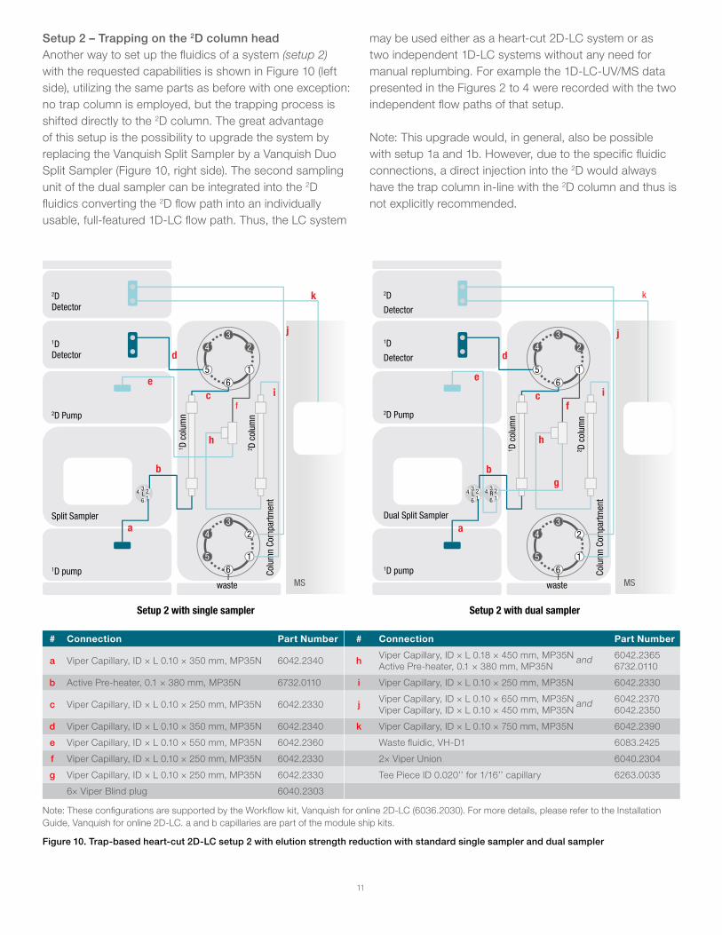
Setup 2 – Trapping on the 2D column headAnother way to set up the fluidics of a system (setup 2) with the requested capabilities is shown in Figure 10 (left side), utilizing the same parts as before with one exception: no trap column is employed, but the trapping process is shifted directly to the 2D column. The great advantage of this setup is the possibility to upgrade the system by replacing the Vanquish Split Sampler by a Vanquish Duo Split Sampler (Figure 10, right side). The second sampling unit of the dual sampler can be integrated into the 2D fluidics converting the 2D flow path into an individually usable, full-featured 1D-LC flow path. Thus, the LC system

Figure 10. Trap-based heart-cut 2D-LC setup 2 with elution strength reduction with standard single sampler and dual sampler

may be used either as a heart-cut 2D-LC system or as two independent 1D-LC systems without any need for manual replumbing. For example the 1D-LC-UV/MS data presented in the Figures 2 to 4 were recorded with the two independent flow paths of that setup.

Note: This upgrade would, in general, also be possible with setup 1a and 1b. However, due to the specific fluidic connections, a direct injection into the 2D would always have the trap column in-line with the 2D column and thus is not explicitly recommended.

L3 2

164

Colu

mn

Com

partm

ent

MS

3

65

4

1

2

3

65

4

1

2

waste

L3 2

164 R

3 216

4

Colu

mn

Com

partm

ent

MS

3

65

4

1

2

3

65

4

1

2

waste

i

a

b

c

d

e

f

h

i

j

k

a

b

e

f

g

h

j

k

c

d1D Detector

2D Detector

Split Sampler

1D pump

2D Pump

1D

Detector

2D

Detector

Dual Split Sampler

1D pump

2D Pump

1 D c

olum

n

2 D c

olum

n

1 D c

olum

n

2 D c

olum

n

Setup 2 with single sampler Setup 2 with dual sampler

# Connection Part Number # Connection Part Number

a Viper Capillary, ID × L 0.10 × 350 mm, MP35N 6042.2340 h Viper Capillary, ID × L 0.18 × 450 mm, MP35N and Active Pre-heater, 0.1 × 380 mm, MP35N

6042.2365 6732.0110

b Active Pre-heater, 0.1 × 380 mm, MP35N 6732.0110 i Viper Capillary, ID × L 0.10 × 250 mm, MP35N 6042.2330

c Viper Capillary, ID × L 0.10 × 250 mm, MP35N 6042.2330 j Viper Capillary, ID × L 0.10 × 650 mm, MP35N and Viper Capillary, ID × L 0.10 × 450 mm, MP35N

6042.2370 6042.2350

d Viper Capillary, ID × L 0.10 × 350 mm, MP35N 6042.2340 k Viper Capillary, ID × L 0.10 × 750 mm, MP35N 6042.2390

e Viper Capillary, ID × L 0.10 × 550 mm, MP35N 6042.2360 Waste fluidic, VH-D1 6083.2425

f Viper Capillary, ID × L 0.10 × 250 mm, MP35N 6042.2330 2× Viper Union 6040.2304

g Viper Capillary, ID × L 0.10 × 250 mm, MP35N 6042.2330 Tee Piece ID 0.020’’ for 1/16’’ capillary 6263.0035

6× Viper Blind plug 6040.2303

Note: These configurations are supported by the Workflow kit, Vanquish for online 2D-LC (6036.2030). For more details, please refer to the Installation Guide, Vanquish for online 2D-LC. a and b capillaries are part of the module ship kits.

12

The system operation of setup 2 with a dual sampler is depicted in Figure 11. Again, the upper switching valve controls the fractionation (A). With the valve in position 6_1 the 1D eluate is directed to the T-piece to be diluted with the 2D flow and trapped on the head of the 2D column (B). The lower switching valve controls if the 2D flow goes to waste or the detectors. During the trapping and washing process it is in position 6_1 to prevent non-volatile salts from entering the MS (B+C). For the 2D analysis it switches to position 1_2 (D). The same valve configuration is used if both flow paths are utilized as independent 1D-LC paths.

Once more, a configuration with both valves in 6_1 must be avoided. One weak point of setup 2 is again a limitation in the applicable flow rates in 2D-LC methods. During the flow combination at the T-piece the pressure in both flow paths increases significantly, flow rates must be selected such that the pressure limits of the columns and the system are not exceeded. The installation of the 1D detector in front of the fractionation valve, like shown with setup 1b, is not recommended for setup 2 because the generated pressure will easily exceed the flow cell limits.

Figure 11. The different stages of heart-cut 2D-LC or direct injection with setup 2 with a dual sampler and the respective valve positions

Action Lower valve Upper valve

A) 1D analysis – 2D idle 6_1 1_2

B) Heart-cut + trapping 6_1 6_1

C) 1D analysis + trap washing 6_1 1_2

D) 1D and 2D analysis 1_2 1_2

D) Direct injection 1D and 2D 1_2 1_2

AVOID 1_2 6_1

1D Detector

2D Detector

Colu

mn

Com

partm

ent

1D Dual Split Sampler

1D pump

3

65

4

1

2

3

65

4

1

2

1 D C

olum

n

2 D C

olum

n

waste

MS

2D Pump

2D Dual Split Sampler

1D Detector

2D Detector

Colu

mn

Com

partm

ent

1D Dual Split Sampler

1D Pump

3

65

4

1

2

3

65

4

1

2

1 D C

olum

n

2 D C

olum

n

waste

MS

2D Pump

2D Dual Split Sampler

1D Detector

2D Detector

Colu

mn

Com

partm

ent

1D Dual Split Sampler

1D Pump

3

65

4

1

2

3

65

4

1

2

1 D C

olum

n

2 D C

olum

n

waste

MS

2D Pump

2D Dual Split Sampler

1D Detector

2D Detector

Colu

mn

Com

partm

ent

1D Dual Split Sampler

1D Pump

3

65

4

1

2

3

65

4

1

2

1 D C

olum

n

2 D C

olum

n

waste

MS

2D Pump

2D Dual Split Sampler

Setup 2 with dual sampler

A) 1D analysis / 2D idle B) Heart-cut with elution strength reduction and trapping

C) Trap washing (optional) D) 1D and 2D analysis

13

Figure 12. Trap-based heart-cut 2D-LC setup 3 with elution strength reduction and dual sampler

Setup 3 – Advanced setup with trap column and flexible usage as 2D-LC or two 1D-LC systemsThe last setup (setup 3) to be presented here is seen in Figure 12. It employs one more column compartment and one more switching valve compared to the former setups but in return overcomes several shortcomings of those and makes use of the upgrade by the dual sampler. The functionality is outlined in Figure 13. Nothing changes for the 1D, so the upper valve again controls the fractionation (A). The left lower valve controls if the 2D flow goes to the T-piece or directly to the right lower valve. The right lower valve determines if the flow goes through the trap column or not. If a 1D fraction is directed to the T-piece, both lower

Colu

mn

Com

partm

ent

L3 2

164 R

3 216

4

Colu

mn

Com

partm

ent

MS

3

65

4

1

2

3

65

4

1

23

65

4

1

2

Trap

waste

a

b

c

d

e

h

i

j

k

l

m

n

f

g

o

Setup 3

1D Detector

2D Detector

Dual Split Sampler

1D pump

2D Pump

1 D c

olum

n

2 D c

olum

n

switching valves are in position 1_2 to mix it with the 2D flow and load it onto the trap column in forward direction (B). For trap washing the position is kept (C), but for the 2D analysis both lower valves switch to position 6_1 to backflush the trap column to the 2D column (D). If a direct injection to the 2D column is done, the left lower valve is in 6_1, but one usually would use the right lower valve in 1_2 (E). However, the trap column can also be switched into the flow to create conditions as present in a 2D-LC run.

Similar to setup 1a vs. 1b, it is possible to install the 1D detector in front of the fractionation valve to detect the 1D during the cut, but again this comes with a trade-off for

# Connection Part Number # Connection Part Number

a Viper Capillary, ID × L 0.10 × 350 mm, MP35N 6042.2340 h Viper Capillary, ID × L 0.10 × 250 mm, MP35N 6042.2330

b Active Pre-heater, 0.1 × 380 mm, MP35N 6732.0110 i Viper Capillary, ID × L 0.10 × 350 mm, MP35N 6042.2340

c Viper Capillary, ID × L 0.10 × 250 mm, MP35N 6042.2330 j Viper Capillary, ID × L 0.18 × 450 mm, MP35N 6042.2365

d Viper Capillary, ID × L 0.10 × 350 mm, MP35N 6042.2340 k Viper Capillary, ID × L 0.10 × 150 mm, MP35N 6042.2320

e Viper Capillary, ID × L 0.10 × 550 mm, MP35N 6042.2360 l Viper Capillary, ID × L 0.10 × 250 mm, MP35N 6042.2330

f Viper Capillary, ID × L 0.10 × 450 mm, MP35N 6042.2350 m Active Pre-heater, 0.1 × 380 mm, MP35N 6732.0110

g Viper Capillary, ID × L 0.10 × 250 mm, MP35N 6042.2330 n Viper Capillary, ID × L 0.10 × 650 mm, MP35N 6042.2370

Waste fluidic, VH-D1 6083.2425 o Viper Capillary, ID × L 0.10 × 750 mm, MP35N 6042.2390

2× Viper Union 6040.2304 Tee Piece ID 0.020’’ for 1/16’’ capillary 6263.0035

6× Viper Blind plug 6040.2303

Note: These configurations are supported by the Workflow kit, Vanquish for online 2D-LC. For more details, please refer to the Installation Guide, Vanquish for online 2D-LC. a and b capillaries are part of the module ship kits.

14

flexibility in flow rate selection as discussed above. Two major advantages of using a second column compartment and a third valve in setup 3 over the previously discussed setups are that the column temperatures of both

dimensions can be set independently and there are no potential valve positions that accidentally feed the 1D mobile phase to the 2D column or MS. Thus, the setup is less prone to user errors.

Figure 13. The different stages of heart-cut 2D-LC or direct injection with setup 3 and respective valve positions

Colu

mn

Com

partm

ent

Colu

mn

Com

partm

ent

3

65

4

1

2

3

65

4

1

2

1 D C

olum

n

3

65

4

1

2

Trap

2 D C

olum

n

waste

1D Detector

2D Detector

1D Dual Split Sampler

1D Pump

MS

2D Pump

2D Dual Split Sampler

Colu

mn

Com

partm

ent

Colu

mn

Com

partm

ent

3

65

4

1

2

3

65

4

1

2

1 D C

olum

n3

65

4

1

2

Trap

2 D C

olum

n

waste

1D Detector

2D Detector

1D Dual Split Sampler

1D Pump

MS

2D Pump

2D Dual Split Sampler

Setup 3

Colu

mn

Com

partm

ent

Colu

mn

Com

partm

ent

3

65

4

1

2

3

65

4

1

2

1 D C

olum

n

3

65

4

1

2

Trap

2 D C

olum

n

waste

1D Detector

2D Detector

1D Dual Split Sampler

1D Pump

MS

2D Pump

2D Dual Split Sampler

Colu

mn

Com

partm

ent

Colu

mn

Com

partm

ent

3

65

4

1

2

3

65

4

1

2

1 D C

olum

n

3

65

4

1

2

Trap

2 D C

olum

n

waste

1D Detector

2D Detector

1D Dual Split Sampler

1D Pump

MS

2D Pump

2D Dual Split Sampler

Colu

mn

Com

partm

ent

Colu

mn

Com

partm

ent

3

65

4

1

2

3

65

4

1

2

1 D C

olum

n

3

65

4

1

2

Trap

2 D C

olum

n

waste

1D Detector

2D Detector

1D Dual Split Sampler1D Pump

MS

2D Pump

2D Dual Split Sampler

A) 1D analysis / 2D idle B) Heart-cut with elution strength reduction and trapping

C) Trap washing (optional)

E) OR direct injection 1D and 2DD) 1D and 2D analysis

Action

Upper valve

L

Lower valve

L

Lower valve

R

A) 1D analysis – 2D idle

1_2 1_2 1_2

B) Heart-cut + trapping 6_1 1_2 1_2

C) 1D analysis + trap washing 1_2 1_2 1_2

D) 1D and 2D analysis 1_2 6_1 6_1

E) Direct injection 1D and 2D

1_2 6_1 1_2

D) Direct injection 1D and 2D with trap in line

1_2 6_1 6_1

15

Comparison of the different setupsFigure 14 gives an overview on the chromatographic performance of all setups for the second flow path in 1D-LC mode as well as in heart-cut 2D-LC mode. The peak areas and widths were independent from the applied instrument setup as well as from the analytical mode. The consistent peak areas confirmed the transfer of complete peaks from the 1D to the 2D. No significant differences in peak widths were found, proving the concept of compound

Table 4. Comparison of the heart-cut 2D-LC setups applying elution strength reduction

Setup 1a Setup 1b Setup 2 Setup 3

Flexible flow rate settings yes no no yes

Direct injection 2D without manual replumbing no no yes yes

Parallel 1D-LC in both flow paths no no yes yes

Trap column in line with 2D column always in line always in line no trap column in- or off- line with 2D column

1D UV detection during heart-cut no yes no no (possible as in setup 1b)

All valve positions prevent 1D eluate to contaminate into MS no no no yes

Equipment 1 column compartment, 2 valves

1 column compartment, 2 valves

1 column compartment, 2 valves

2 column compartments, 3 valves

Different temperature settings for 1D and 2D no no no yes

Figure 14. Comparison of chromatographic results (UV) for the desmedipham peak obtained by 1D-LC (direct injection into second flow path) and heart-cut 2D-LC with the three presented instrument setups (1D-LC in setup 1 was enabled by manual replumbing)

trapping and focusing. Thus, all presented setups are equivalent from a chromatographic point of view and just provide different ways to realize heart-cut 2D-LC with elution strength reduction assisted fraction trapping. The setup selection strongly depends on the application requirements and preferences of the user. All strengths and limitations herein discussed are again summarized in Table 4, highlighting setup 3 as the most favorable system.

16

Moreover, the benefits that arise from the combination of a 2D-LC system with a Vanquish Dual Split Sampler are outlined here:

1. The system is flexible in its use either as two independent 1D-LC flow paths or as one 2D-LC flow path, depending on the current need of the user.

2. No manual modifications are required to switch between both application options.

3. Simplified method development for the 2D in 2D-LC is provided. Due to enabled direct injection, the 2D method can be developed in a 1D way.

4. More efficient instrument utilization is facilitated. If there is no analytical task pending that requires dedicated 2D-LC options, the system can be utilized for more routine work in 1D-LC. This also increases the return on investment (ROI) of the instrument.

5. Similarly, more efficient instrument utilization is possible for MS devices if used as detectors in the setup. Mass spectrometers usage can be increased by running 1D-LC applications if no 2D-LC tasks are pending. This increases the efficiency of the system and ROI.

6. The concept generally can be applied to all kinds of 2D-LC setups (online/offline/heart-cut/multi-heart-cut and comprehensive 2D-LC), depending on the exact fluidic setup.

7. Since the Vanquish Split Sampler can be substituted with a Vanquish Dual Split Sampler, the number of instrument modules required, and thus, the overall instrument size, is the same as for “2D-LC only” instruments. Therefore, the instrument offers more options but with the same instrument size.

8. The instrument size is more compact compared to a solution that utilizes two single autosamplers instead of one dual sampler. The samples for two methods can be stored in one location. This is a major advantage, for example, if a sample needs to be analyzed by complementary 1D-LC methods. It is not necessary to move samples from one location to another.

9. Even more sophisticated workflows are enabled, such as a trapped fraction can be spiked with an internal standard or reagent on the trap column before the 2D analysis is started.

Instrument controlAll presented heart-cut 2D-LC setups were tested under Chromeleon CDS version 7.2.9 as well as under Xcalibur 4.0 software in combination with SII for Xcalibur 1.4 software. Chromeleon is the recommended software for the highest flexibility in 2D-LC method setup due to the exclusive availability of custom columns, custom variables, and intelligent run control (IRC). Switchable instrument usage as one 2D-LC system or as two 1D-LC systems is available under Chromeleon CDS versions from 7.2.8, as the Vanquish Dual Split Sampler is not supported by earlier versions.

System operation is also possible under different software packages. Vanquish modules, including the Vanquish Dual Split Sampler, are supported from SII for Empower 1.0 (Empower 3FR4 required). SII for Xcalibur from version 1.4 supports the Vanquish Dual Split Sampler as well, but not in operation in dual mode, meaning a shared use by two independent 1D-LC instruments. Neither SII for Empower nor SII for Xcalibur provide custom variables or IRC

1D-LC methods in either flow path are set up as usual in Chromeleon CDS or SII software using the instrument method wizard. Depending on the selected configuration, 1D-LC injections may be available in only one or in both flow paths.

An important aspect during 2D-LC method creation is to be aware of the temporal difference between the detection of a 1D peak and its arrival at the cutting valve. The shift can be positive or negative depending on the position of the 1D detector (in front of or behind the valve) and its magnitude may be estimated from the fluidic volumes between the points of detection and cutting and from the 1D flow rate. However, the calculated delay should be seen as a first estimation and experimental confirmation and fine-optimization is recommended when the instrument is installed. If the 1D resolution allows for it, a cutting window broader than the actual peak width could be considered to compensate for minor retention time shifts, especially if quantitative data evaluation is intended. For a dilution-assisted trapping, the flow through the trap column may be ramped up some time before the cut to ensure a sufficient dilution of strong solvent from the 1D and kept up for some time after the cut to wash the trap column (see more in the appendix).

17

In general there are two options to create analytical heart-cut 2D-LC methods:

(1) 1D and 2D analyses are combined in one instrument method, leading to a single data file for each 2D-LC run (as in Figure 8).

(2) The instrument methods for 1D and 2D are separated. Each 2D-LC analysis comprises two steps in the sequence and results in two data files.

Moreover, the user may choose between a hard-coded or smart-coded method setup, if the instrument is under Chromeleon CDS control. The former meaning that the cut times are fixed, and a new instrument method is required for every change in the target heart-cut. This kind of 2D-LC method creation is available with all software packages mentioned above. However, Chromeleon uniquely provides some more extraordinary features that enable for a more flexible and intelligent method setup. These features comprise custom columns in the sequence, custom variables in the instrument method, and intelligent run control (IRC) settings in the processing method.

Although smart-coding appears more complex than hard-coding, it is seen as the superior way to set up heart-cut 2D-LC methods. However, a template created once may be re-used for many other cases. One template is also provided with the current Technical Note online on AppsLab (https://appslab.thermofisher.com/). One drawback compared to the hard-coded option is the longer run time, as the 2D does not start directly after the cut but waits for the 1D to finish. On the other hand, the method is completely flexible in cut selection and thus is applicable for each peak in the considered elution window. Which way is preferred is up to the user and also depends on the software package. Table 5 summarizes the capabilities of the different CDS systems.

Some examples on the addressed aspects and detailed instructions on how to set up the system, instrument methods, and sequences are outlined in the appendix.

Conclusion• The Vanquish UHPLC platform offers several options to

set up heart-cut 2D-LC with elution strength reduction assisted fraction trapping. Such instruments facilitate straightforward peak identity and purity confirmation by mass spectrometry from MS incompatible LC-UV methods in the 1D dimension.

• The most favorable setups employ a Vanquish Dual Split Sampler and provide utilization as either one heart-cut 2D-LC system or as two independent 1D-LC systems without any manual intervention. The flexible operation tremendously increases the instrument’s usability and value.

• Due to its multiple extraordinary features Chromeleon is the preferred CDS software to install and control the instrument. However, working under SII for Xcalibur as well as SII for Empower is possible.

References:1. Guiochon, G. The limits of the separation power of unidimensional column liquid

chromatography, J. Chrom. A 2006, 1126, 6–49.

2. Guiochon, G. et al., Implementations of two-dimensional liquid chromatography, J. Chrom. A 2008, 119, 109–168.

3. Grübner, M.; Steiner, F. Complementary Dual LC as a convenient alternative to multiple heart-cut 2D-LC for samples of medium complexity, Thermo Fisher Scientific Technical Note 73184, 2019, https://assets.thermofisher.com/TFS-Assets/CMD/Technical-Notes/tn-73184-lc-multiheart-cut-alternative-tn73184-en.pdf (accessed October 22, 2019).

4. Stoll, D. R.; Carr, P. W., Two-dimensional liquid chromatography: A state of the art tutorial, Anal. Chem. 2017, 89, 519–531.

5. Petersson, P.; Haselmann, K.; Buckenmaier, S., Multiple heart-cutting two dimensional liquid chromatography mass spectrometry: Towards real time determination of related impurities of bio-pharmaceuticals in salt based separation methods, J. Chrom. A 2016, 1468, 95–101.

6. Stoll, D. R. et al., Evaluation of detection sensitivity in comprehensive two-dimensional liquid chromatography separations of an active pharmaceutical ingredient and its degradants, Anal. Bioanl. Chem. 2015, 407, 265–277.

Table 5. Comparison of the heart-cut 2D-LC setups applying elution strength reduction

ChromeleonXcalibur with SII

for XcaliburEmpower with SII

for Empower

Support of Vanquish Dual Split Sampler

Support of Dual LC

Heart-cut 2D-LC in one method

Heart-cut 2D-LC in separated methods

Custom columns/custom variables

Hard-coded heart-cut 2D-LC

Smart-coded heart-cut 2D-LC

Intelligent Run Control (IRC)

18

Appendix: Instrument configuration, method and sequence setup for Vanquish systems with flexible use in heart-cut 2D-LC or dual 1D-LC modeInstrument configuration2D-LC instrument• For a heart-cut 2D-LC system all involved modules are

configured as one instrument (Figure 15A).

• Avoid double assignments of module and channel names, e.g. rename default “PumpModule” to “PumpModule_1” and default “Pump_Pressure” to “Pump_Pressure_1”. In the special case of two DADs used in one instrument to record UV spectra in both dimensions, the renaming of the channel “3DFIELD” needs to be implemented by a certified service technician.

• If two column compartments are used (setup 3), these must be added as two individual modules, not in combined mode, to ensure that more than two valves can be configured.

• If a dual sampler is installed and the system is to be used for 2D-LC as well as for 1D-LC injections, both sampling units are assigned to that single instrument. When setting up an instrument method with the instrument method wizard, the user selects the injection unit that needs to be active (Figure 15B). Thus 1D-LC analysis in both flow paths is feasible in that configuration, as long as only one sampling unit is active at the same time.

Dual 1D-LC instrument• For full applicability of parallel dual LC, the instrument

configuration has to be converted into two separate instruments, one for every flow path and the sampling units of the dual sampler are assigned to either of them (Figure 15C).

Configuration switch• In practice it is most convenient to prepare both

instrument configuration options and export and store them in an easily accessible place like the computer

desktop. Depending on the current need, the user can import the required configuration with a few clicks without spending a lot of time on rearranging the configuration (Figure 15D).

Instrument method setup1D-LC methods 1D-LC methods in either flow path are set up as usual in Chromeleon CDS or SII software using the instrument method wizard. If a single sampler is installed, 1D-LC is available for the first flow path only. If the dual sampler is installed, both flow paths are ready for 1D-LC injections. If the instrument is configured as dual LC instrument the correct injection unit is already defined prior to method setup. In a 2D-LC instrument configuration the injection unit has to be selected as a first step in the wizard (Figure 15B). The user needs to make sure that all valves are in their proper positions. Switching is usually not required during 1D-LC runs.

2D-LC methods – cut delayFor the current example with setup 3 (see Figure 16), the experimental 1D-LC retention time of the 1D peak was determined as 3.78 min with a peak start at 3.73 min and a peak end at 3.86 min. Due to the positioning of the 1D detector after the cutting valve, a proper heart-cut needs to be executed before the peak reaches the detector but at the time it reaches the valve. The respective negative delay can be derived from the fluidic volumes between valve and detector and the 1D flow rate. Here the most considerable volume contribution comes from the 1D detector. From the specifications in the operating manual one can find a sum of ~50 µL illuminated and inlet volume for the utilized detector flow cell, translating into a delay of ~0.08 min for a flow rate of 0.6 mL/min. Thus, the heart-cut was set from 3.65 min to 3.78 min in order to capture the whole peak. Good results were achieved as the peak heights and areas in the 2D did not differ from a direct 1D-LC injection. Nevertheless, the calculated delay should be seen as a first estimation and experimental confirmation and fine-optimization is recommended.

19

Figure 15. Instrument configurations (A, C), instrument method wizard (B), and desktop symbols (D)

2D-LC methods – Example 1: one instrument method comprising 1D and 2D with hard-coded cut• Most important method aspects for setup 3 are shown in

Figure 16.

• For the 1D gradient there is no change except in the re-equilibration time.

• The switching times of the upper valve are set to 3.65 min and 3.78 min according to the previous cut delay calculation.

• The 2D pump flow through the trap column is increased some time before the heart-cut (3.0 min) to ensure a sufficient dilution of strong solvent from the 1D and is kept up for some time after the cut to wash the trap column (4.3 min).

• The 2D pump flow ramp settings in the script editor should be considered carefully to make sure that the flow is up when the 1D fraction arrives and down when the 2D column is switched in line to start the 2D run.

• The 2D gradient starts at 4.5 min (pump gradient starts and both lower valves switch), thus the gradient times are shifted accordingly compared to Table 2.

• The cut times are fixed/hard-coded. A new instrument method is required for every change in the target heart-cut. This kind of 2D-LC method creation is available with all software packages mentioned above.

A

DC

B

20

Figure 16. Important heart-cut 2D-LC instrument method aspects when programmed as one hard-coded instrument method for setup 3 (examplary methods are availiable with this Technical Note online at https://appslab.thermofisher.com/)

2D start

Heart-cut

C

Increased flowthrough trap

1D gradient

21

2D-LC methods – Example 2: separate instrument methods for 1D and 2D with smart-coded cut• Prior to the actual instrument method creation, create

“custom columns” in the sequence table to enter individual cut times:

– Right-click into the sequence table header, choose “Custom Columns” and “Insert Custom Variable”. In the window that opens click “Create a new custom variable”, select a name like “CutStart” or “CutEnd”, type is “numeric”, check “allow empty values”, minimum is 0, maximum depends on the run time, unit is usually “min”, precision should be not less than 2. Two custom columns are needed to define the cut start and end.

• Example instrument methods are depicted in Figure 17 and Figure 18. The first method contains the 1D gradient, the cut and trap process, as well as the trap washing. The second method contains the 2D gradient and the 1D flushing and re-equilibration.

• The smart-coding only affects the 1D method. Here, the 1D gradient is programmed up to the time one can expect peaks to elute (gradient delay should be considered), the valves and the 2D pump are just set to the starting conditions.

• All further events are implemented by triggers in the script editor (Figure 17). Four triggers, which refer to the previously created custom variables, are entered into the Start Run stage at 0 min: two to increase or decrease the flow rate of the 2D pump (“FlowUp” and “FlowDown” in Figure 17) and two to start and end the fractionation (“CutStart” and “CutEnd” in Figure 17):

– Click the line before where you want to insert a trigger block and then click in the “Insert” section of the ribbon “Conditional” and “Insert Trigger”. For each trigger a unique name is entered in double quotation marks and a condition is compiled in the style of “System.Retention>=System.Injection.CustomVariables.[name e.g. CutStart or CutEnd]±X”, the limit is set to 1 (maximum execution once per run) and finally the action is entered, i.e. flow rate is set or valve position is set. “X” in the condition can be 0 or for example -0.5 to increase the flow rate 0.5 min before the cut.

• “X” could also serve for the automated correction of the delay between detected peak start/end and required valve action (in the current case -0.08 min as above, not applied in Figure 17). With that the user could just enter the times detected in a 1D-LC analysis without manual calculation.

• The second method starts in the initial stage at the conditions at which the first method ends. At the 0 min stage both lower valves switch their position and the 2D gradient starts (see Figure 18).

• A complete heart-cut 2D-LC analysis comprises an injection with the first method with target cut times entered into the created custom columns in the sequence table and a blank injection with the second method (Figure 19).

• The latter one can be either added to the sequence manually or automatically if a processing method using “intelligent run control” (IRC) is applied. This Chromeleon CDS feature facilitates, for example, the insertion of an injection as soon as a current injection is finished:

– In the processing method enter the SST/IRC tab, click to the table to add a new test case and check “Create an unconditional test case”. Enter a name. For the conditions check “Injection property” and enter “Inject InstrumentMethod”, “=” and “[name of 1D method]” (see Figure 19). In the action section add “Insert Injection” and browse for a source of an appropriate injection (must be a blank injection with the respective 2D instrument method).

22

Figure 17. Important heart-cut 2D-LC instrument method aspects when programmed as separate instrument methods for setup 3; 1D method with smart-coded heart-cutting (examplary methods are availiable with this Technical Note online at https://appslab.thermofisher.com/)

Triggers for heart-cut

C

Valves at starting conditions

1D gradient2D idle

Triggers for trap flow

23

Figure 18. Important heart-cut 2D-LC instrument method aspects when programmed as separated instrument methods for setup 3; 2D method

C

Lower valves switch at start

1D flush and equilibration 2D gradient

For Research Use Only. Not for use in diagnostic procedures. © 2019 Thermo Fisher Scientific Inc. All rights reserved. All trademarks are the property of Thermo Fisher Scientific and its subsidiaries. This information is presented as an example of the capabilities of Thermo Fisher Scientific Inc. products. It is not intended to encourage use of these products in any manners that might infringe the intellectual property rights of others. Specifications, terms and pricing are subject to change. Not all products are available in all locations. Please consult your local sales representative for details. TN73298-EN 1219S

Find out more at thermofisher.com/vanquish

Figure 19. Sequence setup with two separated instrument methods and with IRC wizard