fixed income and credit risk lecture 1
TRANSCRIPT
Fixed Income and Credit Risk
Lecture 1
Professor Assistant ProgramFulvio Pegoraro Roberto Marfe MSc. Finance
Fall Semester 2012
Fixed Income and Credit Risk
Lecture 1
Fixed Income Markets and Securities

Outline of Lecture 1
1.1 Fixed Income and Credit Risk: Introduction
1.2 Fixed Income Markets and Securities
1.2.1 The Government Debt Markets
1.2.2 The Money Market
1.2.3 Federal Funds Rate and Eurosystem Rates
1.2.4 LIBOR, EURIBOR and EONIA
1.2.5 The REPO Market
3

1.3 Basics of Fixed Income Securities
1.3.1 Time value of money
1.3.2 Discount Factors: Bonds
1.3.3 Bond market conventions
1.3.4 Bond yields and zero-coupon rates
1.3.5 Forward rates
4

1.3.6 Forward Rates and Forward Discount Factors
1.3.7 Par yields
1.3.8 Inflation-indexed bonds
5
1.1 FIXED INCOME AND CREDIT RISK: INTRODUCTION
• The purpose of this course is to present ”methods” (principle/models) to deter-
mine the ”fair price” of fixed income securities with and without ”credit risk” as
well as fixed income derivatives and credit derivatives.
• What the class of fixed income securities includes ? It includes, for sure, securities
where the issuer promises one or several FIXED, PREDETERMINED payments
at given points in time.
Examples : Zero-coupon bonds, Coupon bonds.
6

→ when the issuer is a national government, the asset is (in general) assumed to
be non-defaultable (absence of credit risk).
→ bonds are also issued by other institutions like banks and companies: we have
corporate bonds with a positive probability of default (credit risk!).
• We will also consider other financial assets in that class, even if their payoffs are
not fixed and known at the time they are purchased (interest rate derivatives).
Why ? Because that payoffs depend on the price of some ”basic” fixed income
security.
Examples : Options and futures on bonds or interest rates, caps and floors,
swaps and swaptions.
7
• The prices of fixed income securities are frequently expressed in terms of interest
rates or yields ⇒ it is important to understand what’s behind the dynamics of
interest rates in order to understand how to correctly price that assets.
• The fundamental concept in the analysis of fixed income securities is the term
structure of interest rates (also called yield curve).
• The interest rate on a loan will depend in general on the maturity date of that
loan ⇒ differences between short-term and long-term interest rates.
• the term structure of interest rates defines the relationship between the interest
rate and the maturity of the loan.
8

1.2 FIXED INCOME MARKETS AND SECURITIES
• Debt markets have expanded a lot in the last two decades. Now relevant issuers
include:
a) Treasury (Sovereign) Securities: Issued by governments (USA, Japan, UK,
etc.);
b) Agency Securities: Debt securities issued by government agencies, such as
the Federal Home Loan Bank (FHLB), the Tennessee Valley Authority (TVA),
the Federal National Mortgage Association (FNMA) and Government National
Mortgage Association (GNMA).
9

c) Corporate Securities: Debt securities issued by corporations (both investment
grade and noninvestment grade).
d) Mortgage-Backed Securities: Debt securities backed by pools of mortgages.
e) Asset-Backed Securities: Securities backed by a portfolio of assets, such as
credit card receivables.
f) Municipal issues: Debt securities issued by state gov. and municipalities.
g) Derivative Securities: Interest rate Swaps, Forwards, Options, Futures.
↪→ backed by = collateralized by = guaranteed by ;
10
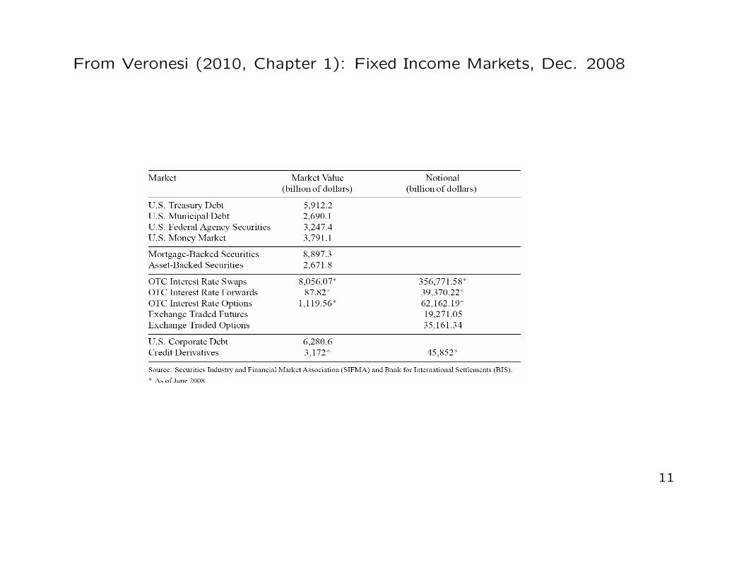
From Veronesi (2010, Chapter 1): Fixed Income Markets, Dec. 2008
11
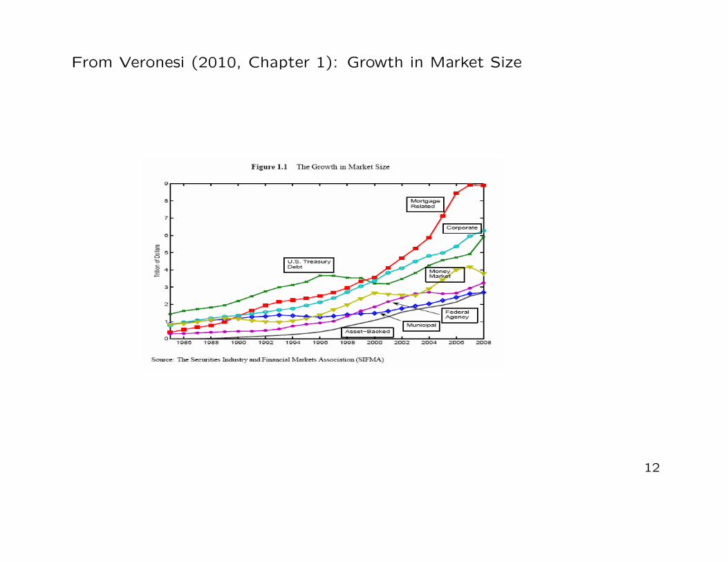
From Veronesi (2010, Chapter 1): Growth in Market Size
12
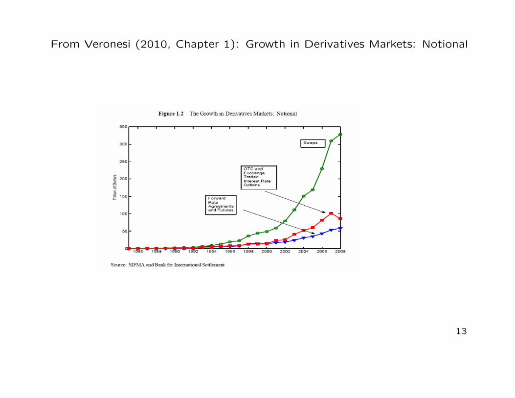
From Veronesi (2010, Chapter 1): Growth in Derivatives Markets: Notional
13

1.2.1 The Government Debt Markets
• The simplest fixed income securities are BONDS.
• A bond is a tradeble loan agreement in which the issuer sells a contract promising
the holder a predetermined payment schedule.
• These payments may be fixed in nominal terms (a fixed-interest bond) or they
may be linked to some index (an index-linked bonds) like the Consumer Price
Index (CPI).
→ We have :
14

� Zero Coupon Bonds: securities that only pay the principal at maturity (T-bills).
� Fixed Rate Coupon Bonds: securities that pay a fixed coupon over a given
period (semiannually) plus the principal at maturity (T-notes and T-bonds).
� Floating Rate Coupon Bonds: securities that have the coupon indexed to
some other short term interest rate, varying over time. The U.S. government
does not issue floating rate bonds, other governments do. For instance, Italy
issues the CCT bond, which is an Italian Treasury debt security whose coupon
rate is indexed to the 6 month rate of Italian 6-month T-bills (BOT).
15

� Treasury Inflation Protected Securities (TIPS): securities with the principal
indexed to inflation, so that coupon payments move accordingly.
• Treasury bills, bonds and notes (in the U.S. bond market), or gilt-edged securities
(in the UK market) provide fixed nominal payments; treasury inflation-protected
securities (TIPS; in the U.S. bond market) provide interest rate payments that
rise with inflation and fall with deflation (measured by CPI).
i) Treasury bills (or T-bills) mature in one year or less, and they do not pay interest
prior to maturity. Regular weekly T-bills are commonly issued with time-to-
maturity of 28 days, 91 days, 182 days, and 364 days.
16
ii) Treasury notes (or T-notes) mature in 2 to 10 years. They have a coupon
payment every six months and are commonly issued with time-to-maturities of
2, 3, 5, 7 or 10 years.
iii) Treasury bonds (or T-bonds) have the longest time-to-maturity, from 20 to 30
years, and they have a coupon payment every six months.
iv) TIPS are currently offered in 5-year, 10-year and 20-years of time-to-maturity.
They have a coupon payment every six months : the coupon rate is constant but
generates a different amount of interest when multiplied by the inflation-adjusted
principal (also named face value or par value).
17
• We also have:
� Separate Trading of Registered Interest and Principal of Securities (STRIPS):
Artificial zero coupon bonds constructed by stripping off separate interest and
principal payments from a coupon bond.
� The Municipal Debt Market
18

From Veronesi (2010, Chapter 1)
19

1.2.2 The Money Market
• Market for short-term borrowing and lending of banks and financial institutions:
� Federal Funds (FF) Rate: rate for borrowing / lending balances kept at the
Federal Reserve[see Section 1.2.3].
� EONIA (Euro Overnight Index Average): it can be seen the Euro Area
banking system equivalent of the effective Federal Funds rate [see Section 1.2.4].
� LIBOR and EURIBOR: average interest rate the banks charge to each other
for short term uncollateralized borrowing / lending [see Section 1.2.4].
20
� Repo Rate: interest rate charged for short term borrowing / lending with
collateral [see Section 1.2.5].
� Eurodollar Rate: it is the rate of interest on a dollar deposit in a European-
based bank. These are short-term deposits from 3 months to one year. In
particular, the 90-day Eurodollar rate has become a standard reference to gauge
conditions of the interbank market (see following lectures). For instance:
– the market of Eurodollar futures and options (financial derivatives traded at
the Chicago Mercantile Exchange that allow financial institutions to bet on
or hedge against the future evolution of the Eurodollar rate) is among the
largest and most liquid derivative markets in the world.
21
1.2.3 Federal Funds (FF) Rate and Eurosystem Rates
• In the U.S. banks and other institutions must keep some amount of capital (called
federal funds) within the Federal Reserve (U.S. system of central banks).
– Banks with a reserve surplus may then lend some of their reserves to banks
with a reserve deficit, on a uncollateralized basis.
– The Federal Funds Rate is the interest rate at which banks actively trade
the federal funds with each other, usually overnight.
– The Effective Federal Funds (EFF) rate is the volume-weighted average
rate that banks charge to each other to lend or borrow reserves at the Fed.
22
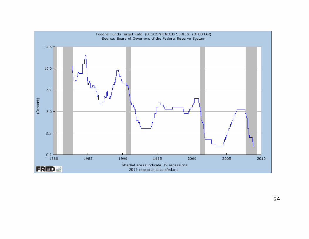
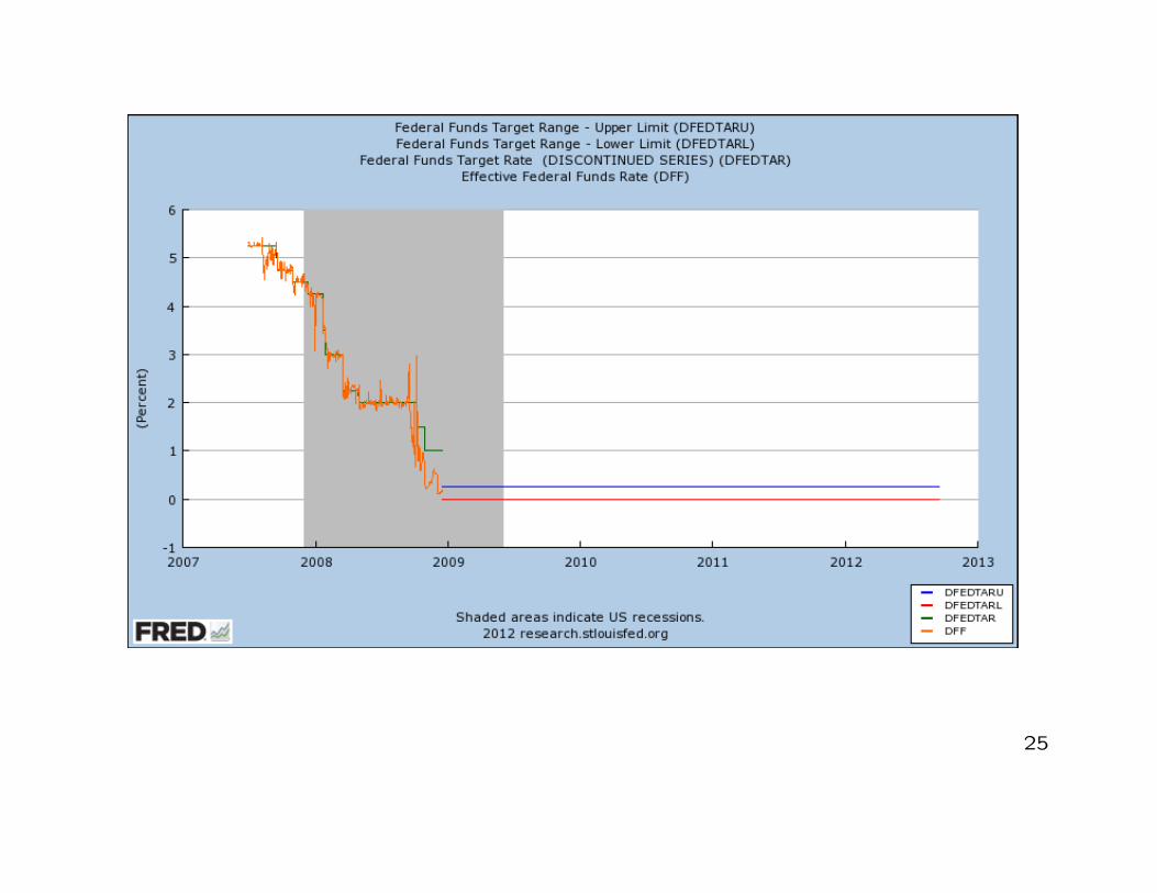
• The Federal Funds Target (FFT) Rate is determined by a meeting of the
members of the Federal Open Market Committee (FOMC) which normally
occurs eight times a year about seven weeks apart. The FOMC may also hold
additional meetings and implement target rate changes outside of its normal
schedule.
– The Fed uses open market operations (OMO) (buy/sell government bonds
on the open market) to influence the supply of money in order to drive the
EFF rate close to the FFT rate.
– The FFT rate is also known as the neutral (or nominal) federal fund rate.
– Since December 16, 2008, the FOMC has fixed a target range 0%− 0.25%.
23
24
25
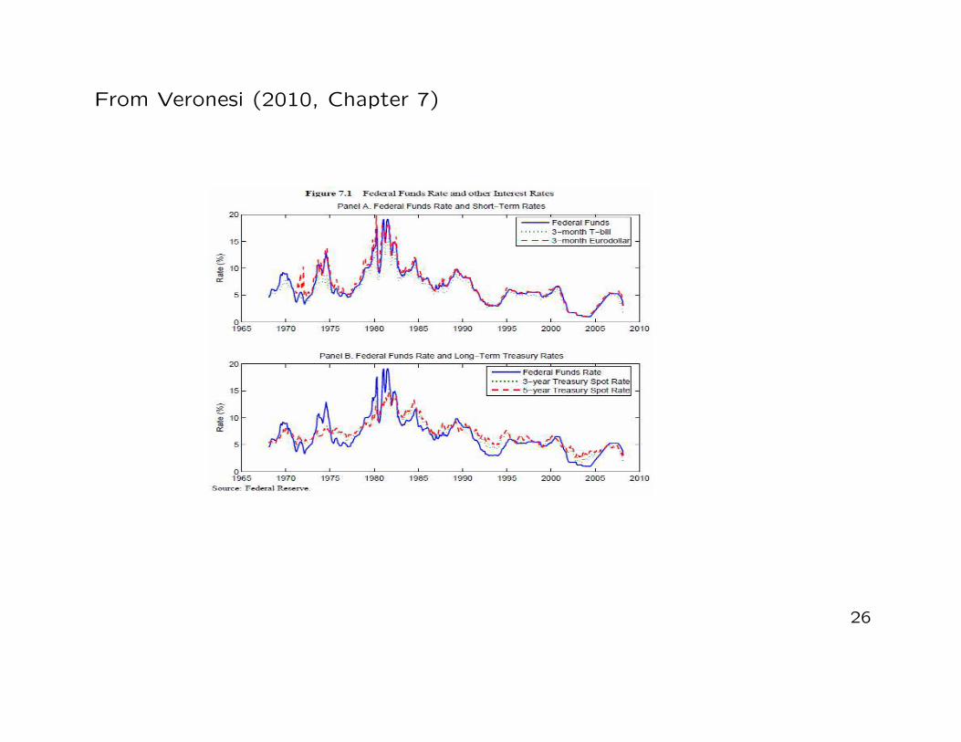
From Veronesi (2010, Chapter 7)
26
� Contrary to the Fed (or the Bank of England and the Swiss National Bank), the
ECB does not have an explicit interest-rate target.
• However, its aim is explicitly to ”influence money market conditions and steer
short-term interest rates” (ECB, 2011).
• In order to influence short-term money market rates, a shortage of liquidity is
determined by imposing reserves to Euro area banks.
→ they are required to hold compulsory cash deposits on accounts with the
Eurosystem, and these requirements are based on the amount and profile of
liabilities standing out from the banks balance sheet at the end of each month.
27
• At the same time, banks in the Eurosystem can refinance themselves through
the ECBs weekly Main Refinancing Operations (MROs).
• In these refinancing operations, the ECB returns (provides) liquidity to the mar-
ket, by allowing banks to tender for cash, against collateral.
• The Euro area equivalent of the FFT rate is European Central Bank’s weekly
Main Refinancing Operation (MRO) rate. Changes in the policy rate are de-
cided during the first of the bimonthly meetings of the ECBs Governing Council.
28
� Since October 2008, in a financial crisis framework, the Eurosystem adopted a
fixed-rate full allotment (FRFA) tender procedure: in other words, the ECB
accommodates any demand for liquidity of bank counterparties at the MRO rate
(against eligible collateral) in unlimited amounts.
• In the Eurosystem we observe two additional policy rates forming a symmetric
corridor around the main policy (MRO) rate:
– the lower bound of the corridor, named deposit-facility rate, is the rate at
which counter-parties can deposit funds overnight in the Eurosystem.
– the upper bound of the corridor, named lending-facility rate, is the rate at
which counter-parties can borrow funds overnight from the Eurosystem.
29

1.2.4 LIBOR, EURIBOR and EONIA
� LIBOR stands for London Interbank Offered Rate.
• Definition: The rate at which an individual Contributor Panel bank could borrow
funds, were it to do so by asking for and then accepting inter-bank offers in
reasonable market size, just prior to 11:00 London time.
• In other words, the bank provide (submit) the rate at which it could borrow
unsecured cash from another bank.
• This rate thus represents the bank’s perception of its cost of funds in the inter-
bank market.
30

• Technical features: LIBOR is calculated and published by Thmson and Reuters
on behalf of the British Banker’s Association (BBA). Each day, the BBA surveys
a Panel of banks asking the question implicit in the above mentioned definition.
• Given the submitted rates, BBA eliminate the highest and the lowest 25% and
average the remaining 50%. This average rate is the published (at around 11:45
London time) Libor rate.
• This rate is calculated for 10 different currencies (U.S. and Canadian dollar,
British Pound, Euro, Japanese Yen, Swiss Franc, ...) across 15 maturities from
the over-night to 1 year.
31

• The number of banks in the Panel is different depending on the concerned
currency: we have 18 banks for the US Dollar Libor, 16 banks for the British
Pound and 15 for the Euro.
• The update of the banks in the Panel is made twice a year by BBA with the
Foreign Exchange and Money Markets Committee (FXMMC). Contributor banks
are selected for currency panels in line with three principles:
1) scale of market activity,
2) credit rating and
3) perceived expertise in the currency concerned.
32

• In the case of the USD Libor, among the contributor banks we have Bank of
America, BNP Paribas, Citibank, Credit Agricole, Credit Suisse and HSBC.
• The Libor is widely used as a reference rate for many financial instruments
(interest rates derivatives): Forward rate agreements (FRA), Interest rate futures
(e.g., Eurodollar futures), Interest rate swaps/options/cap/floor.
33
� EURIBOR stands for Euro Interbank Offered Rate and is produced by the Eu-
ropean Banking Federation (EBF) since 1999.
• Definition: It is the rate at which Euro interbank term deposits within the Euro
zone are offered by one Prime Bank to another Prime Bank. It is computed as
an average of daily quotes provided for fifteen maturities by a panel of 43 of
the most active Banks in the Euro zone. It is quoted on an act/360 day count
convention, and is fixed at 11:00am [CET] displayed to three decimal places..
• Banks in the EURIBOR panel are thus asked to submit rates that reflect the
”best” lending rates in unsecured cash transactions that could take place in the
euro area between the ”best banks”.
34

• The rates submitted by the panel banks are therefore, by definition, independent
of the situation of the banks submitting those rates or of actual transactions in
which they engage.
• EURIBOR is calculated as a trimmed average since the average of the contri-
butions is calculated after eliminating the 15% highest and lowest contributions.
The daily calculation is performed by Thomson Reuters on behalf of the EBF.
– The banks that belong to the panel have been selected to ensure that the
diversity of the euro money market is adequately reflected and are banks
which are ”top-rated by international rating agencies”.
– Banks provide daily quotes in euros for 15 maturities from 1 week to 1 year.
35

• Panel banks are the banks with the highest volume of business in the euro area
money markets and it is made up of:
1) banks from EU countries participating in the euro from the outset;
2) banks from EU countries not participating in the euro from the outset and;
3) large international banks from non-EU countries but with important euro
zone operations.
• Among these banks, we have: BNP-Paribas (FR), HSBC France (FR), Societe
Generale (FR), Deutsche Bank (DE), Commerzbank (DE), Barclays Capital
(UK), Citibank, J.P. Morgan Chase Co, Bank of Tokyo Mitsubishi.
36
� Since April 2012, the EBF has also started to produce a USD EURIBOR reference
which consists of contributions from a panel of 20 banks consisting of banks from
both EU countries and some large international banks from non-EU countries.
According to the EBF, USD EURIBOR is...
• Definition: ... the rate at which USD interbank term deposits are being offered
by one panel bank to another panel bank at 11.00 a.m. Brussels time. All
maturities, other than overnight, are quoted for spot value and on an actual /
360 day basis.
37
• The choice of banks quoting for USD Euribor is based on market criteria. These
international and European banks are of first class market standing and they
have been selected to ensure that the diversity of the European US dollar money
market is adequately reflected.
• The definition of USD EURIBOR is therefore also different from that of EUR
EURIBOR as the first explicitly links the rates being submitted by the panel
banks to their own situation, whereas the second does not. USD EURIBOR,
however, is not yet widely used or known in the market.
38
� EONIA stands for Euro Overnight Index Average. According to the EBFs:
• Definition: It is an an effective overnight rate computed as a weighted average
of all overnight unsecured lending transactions in the interbank market, initiated
within the euro area by the contributing panel banks. Daily reports are provided
by the same panel of 43 banks that contribute to the EURIBOR panel. EONIA
is calculated by the ECB between 6:45 pm and 7:00 pm (CET) and displayed to
three decimal places.
• It is one of the two benchmarks for the euro area money market with the Euribor.
39
3,00
4,00
5,00
6,00
7,00
Ra
tes
MRO, Deposit/Landing-Facility and EONIA rates
MRO Rate
Lending-Facility Rate
Deposit-Facility Rate
0,00
1,00
2,00
01
/02
/19
99
01
/07
/19
99
01
/12
/19
99
01
/05
/20
00
01
/10
/20
00
01
/03
/20
01
01
/08
/20
01
01
/01
/20
02
01
/06
/20
02
01
/11
/20
02
01
/04
/20
03
01
/09
/20
03
01
/02
/20
04
01
/07
/20
04
01
/12
/20
04
01
/05
/20
05
01
/10
/20
05
01
/03
/20
06
01
/08
/20
06
01
/01
/20
07
01
/06
/20
07
01
/11
/20
07
01
/04
/20
08
01
/09
/20
08
01
/02
/20
09
01
/07
/20
09
01
/12
/20
09
01
/05
/20
10
01
/10
/20
10
01
/03
/20
11
01
/08
/20
11
01
/01
/20
12
01
/06
/20
12
Deposit-Facility Rate
EONIA Rate
40
4
5
6
7
8
Ra
te
s3-Month USD LIBOR
3M USD Libor
0
1
2
3
01
/02
/19
99
01
/07
/19
99
01
/12
/19
99
01
/05
/20
00
01
/10
/20
00
01
/03
/20
01
01
/08
/20
01
01
/01
/20
02
01
/06
/20
02
01
/11
/20
02
01
/04
/20
03
01
/09
/20
03
01
/02
/20
04
01
/07
/20
04
01
/12
/20
04
01
/05
/20
05
01
/10
/20
05
01
/03
/20
06
01
/08
/20
06
01
/01
/20
07
01
/06
/20
07
01
/11
/20
07
01
/04
/20
08
01
/09
/20
08
01
/02
/20
09
01
/07
/20
09
01
/12
/20
09
01
/05
/20
10
01
/10
/20
10
01
/03
/20
11
01
/08
/20
11
01
/01
/20
12
01
/06
/20
12
41
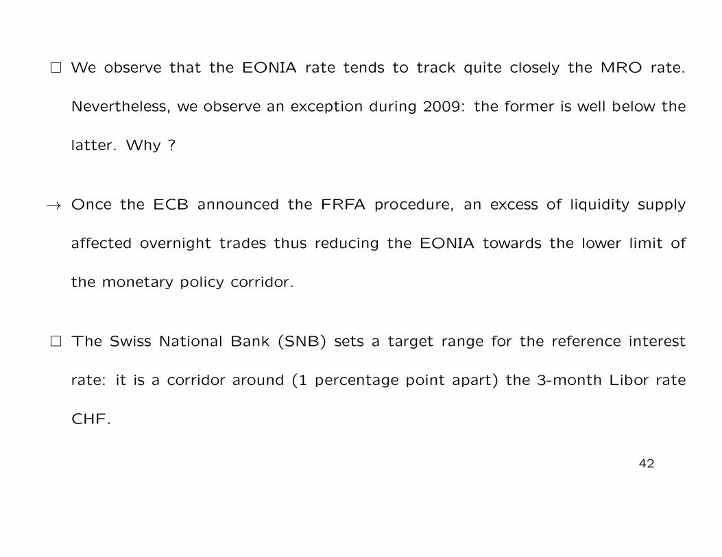
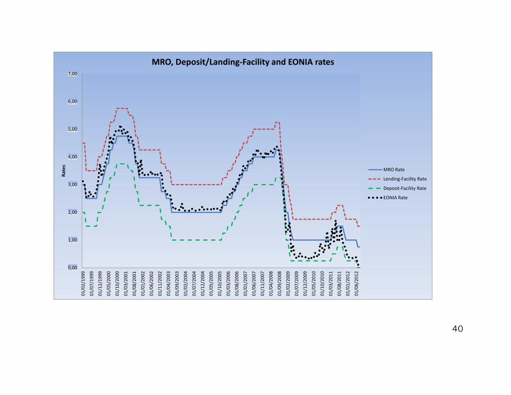
� We observe that the EONIA rate tends to track quite closely the MRO rate.
Nevertheless, we observe an exception during 2009: the former is well below the
latter. Why ?
→ Once the ECB announced the FRFA procedure, an excess of liquidity supply
affected overnight trades thus reducing the EONIA towards the lower limit of
the monetary policy corridor.
� The Swiss National Bank (SNB) sets a target range for the reference interest
rate: it is a corridor around (1 percentage point apart) the 3-month Libor rate
CHF.
42
1.2.5 The REPO Market
� A Repurchase Agreement (Repo) is an agreement to sell (today) some secu-
rities to another party and buy them back at a fixed future date and for a fixed
amount:
→ the price at which the security is bought back is greater than the selling price
and the difference implies an interest called Repo Rate;
→ it can be seen as a collateralized loan. The advantage of this borrowing of funds
is that the applied (Repo) rate is less than the cost of banking financing.
43

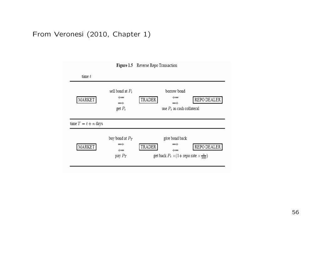
� A Reverse Repo is the opposite transaction, namely, it is the purchase of the
security for cash with the agreement to sell it back to the original owner at a
predetermined price, determined, once again, by the Repo Rate.
→ it is the same repurchase agreement from the repo dealer’s viewpoint, not
the trader’s.
� Repo Scheme: A trader would like to take at date t a long position (buy!) until
date T > t on a given amount of 30-year Treasury bonds.
↪→ Where does the trader obtains the funds to finance (a large part of) this
position?
Let Pt denotes the price of that bond at date t.
44
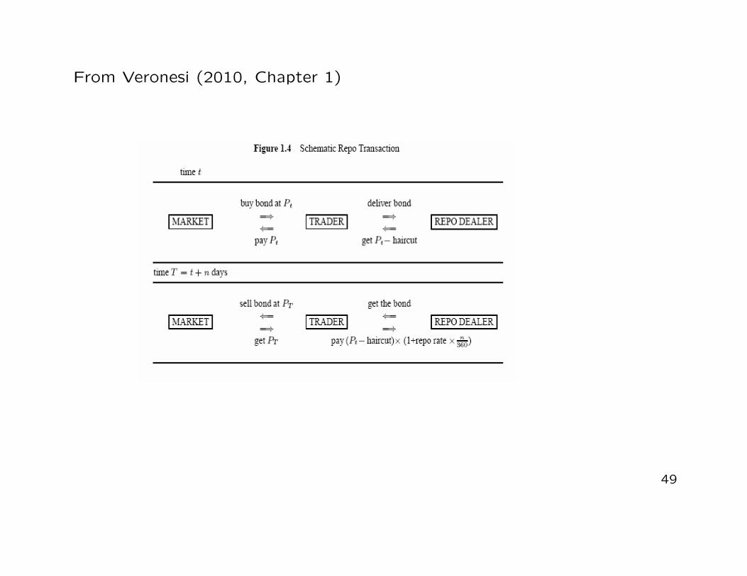
Date t (Opening Leg). The trader enters a repurchase agreement with a repo
dealer:
– the repo dealer gives to the trader the needed cash to buy the bond
– the trader delivers the bond (just bought) as a collateral to the repo dealer;
– in fact, the repo dealer typically gives something less than the market price
Pt of the bond, namely Pt− haircut, where the haircut implicitly discount the
riskiness of the trader (default);
– the trader and the repo dealer agree that the trader will return back the
amount borrowed, (Pt − haircut), plus the repo rate.
45
T = t+n (Closing Leg). The trader gets back the bond from the repo dealer:
– the trader sells the bond in the market to get PT and pays Pt − haircut plus
the repo interest to the repo dealer, where:
repo interest =n
360× repo rate × (Pt − haircut) ,
where n = T − t and 360 is the day count convention in the repo market.
– The profit to the trader is then PT − Pt − repo interest while:
return on capital for trader =PT − Pt − repo interest
haircut
being only the haircut (the margin) the trader’s own capital used in the repo.
46

� It is important to remember that:
– the term T of the repo transaction is decided at t; most of the agreements
are for a very short term, mainly overnight (i.e., one day; it is called overnight
repo). However, we have also longer-term agreements reaching 30 days or
even more (called term repo);
– the repo rate is decided at t;
� The trade implies:
– a positive carry if the return on the bond is above the repo rate;
– a negative carry if the return on the bond is below the repo rate.
47
� It is also important to highlight the following point: legal title to the bond passes
from the trader to the repo dealer.
• Nevertheless, coupons provided by the bond, when the repo dealer owns that
asset, are usually passed directly to the trader.
• The agreement might anyway provide that the repo dealer receives the coupons,
with the cash payable on repurchase being adjusted to compensate.
48
From Veronesi (2010, Chapter 1)
49
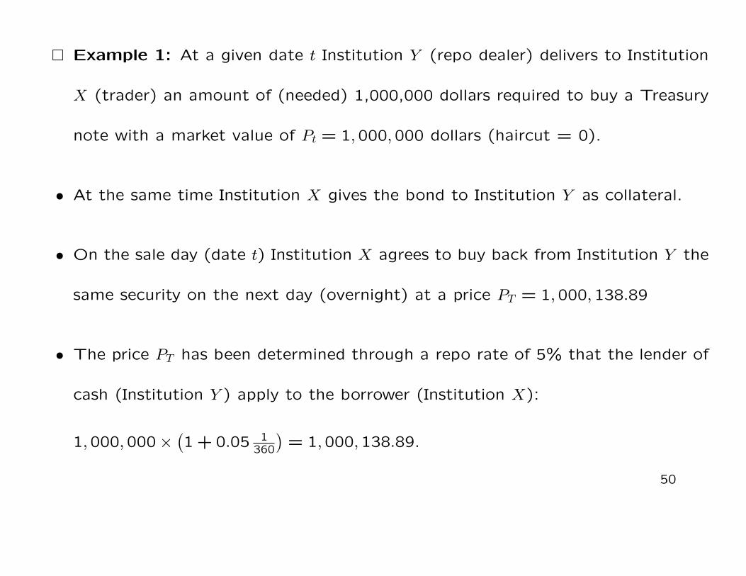
� Example 1: At a given date t Institution Y (repo dealer) delivers to Institution
X (trader) an amount of (needed) 1,000,000 dollars required to buy a Treasury
note with a market value of Pt = 1,000,000 dollars (haircut = 0).
• At the same time Institution X gives the bond to Institution Y as collateral.
• On the sale day (date t) Institution X agrees to buy back from Institution Y the
same security on the next day (overnight) at a price PT = 1,000,138.89
• The price PT has been determined through a repo rate of 5% that the lender of
cash (Institution Y ) apply to the borrower (Institution X):
1,000,000×(1 + 0.05 1
360
)= 1,000,138.89.
50
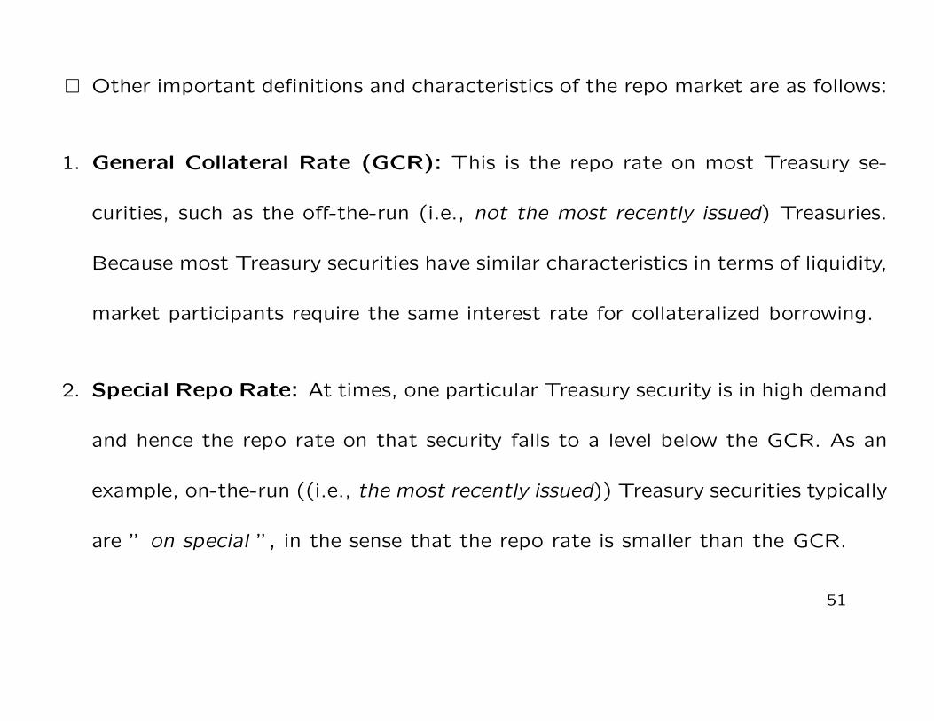
� Other important definitions and characteristics of the repo market are as follows:
1. General Collateral Rate (GCR): This is the repo rate on most Treasury se-
curities, such as the off-the-run (i.e., not the most recently issued) Treasuries.
Because most Treasury securities have similar characteristics in terms of liquidity,
market participants require the same interest rate for collateralized borrowing.
2. Special Repo Rate: At times, one particular Treasury security is in high demand
and hence the repo rate on that security falls to a level below the GCR. As an
example, on-the-run ((i.e., the most recently issued)) Treasury securities typically
are ” on special ”, in the sense that the repo rate is smaller than the GCR.
51
� For which reason a security which is high in demand entail a lower (special) repo
rate ? To understand the logic, consider the next example which considers the
reverse repo.
• Reverse Repo Scheme: Let us consider an investor who thinks that a partic-
ular bond, such as the on-the-run 30-year treasury bond, is overpriced and wants
to take a bet that its price will decline in the future.
– If the trader does not have the bond to sell outright, then he/she can enter
into a reverse repo with a repo dealer to obtain the bond to sell.
52
• More specifically, in a reverse repo, the trader at date t (Opening Leg):
(A) borrows the security (the bond) from the dealer;
(B) sells it in the market at the price Pt;
(C) use Pt as cash collateral for the repo dealer
• Here, the trader is lending money to the repo dealer, against the bond, and thus
he is entitled to receive the repo rate.
53
• At date T = t+ n (Closing Leg), the trader:
– buys the bond in the market paying the price PT ;
– gives the bond back to the repo dealer;
– obtains from the repo dealer Pt × (1 + repo rate× n360
).
• The profit of the trader is (Pt − PT) + repo interest, where:
repo interest =n
360× repo rate × Pt .
54
� Example 2: At a given date t Institution X borrows a Treasury note with a
market value of Pt = 1,000,000 dollars to Institution Y and delivers to Institution
Y 1,000,000 dollars of cash as collateral.
• On the sale day (date t) Institution X agrees to sell back to Institution Y the same
security on the next day (overnight) at a price PT = 1,000,138.89, determined
through a repo rate of 5% that the lender of cash (Institution X) apply to the
borrower of cash (Institution Y )
• Institution X is said to have a reverse repo position. It has effectively a short
position in the Treasury note. Indeed, the profitability of Institution X (bond
trader) goes up when the Treasury note price goes down (Pt > PT).
55
From Veronesi (2010, Chapter 1)
56

• Now, the trader who wants to speculate on the decrease in the bond price, is
happy to accept a reduction of the repo rate in order to get hold of the bond
and realize his/her trading strategy.
• If many traders want to undertake the same strategy of shorting that particular
bond, then the bond is high in demand (to repo dealers) and, thus, the repo
rate for that bond declines below the general collateral rate. The bond is said
to be on special.
• Since borrowing is collateralized by the value of the asset, the repo rate is lower
than other borrowing rates available to banks, such as the (more risky, being
non collateralized) Libor. It is higher than (risk-less) Treasury rates.
57

From Veronesi (2010, Chapter 1)
58
1.3 BASICS OF FIXED INCOME SECURITIES
1.3.1 Time value of money
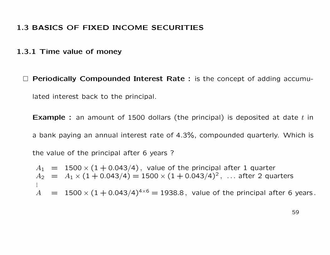
� Periodically Compounded Interest Rate : is the concept of adding accumu-
lated interest back to the principal.
Example : an amount of 1500 dollars (the principal) is deposited at date t in
a bank paying an annual interest rate of 4.3%, compounded quarterly. Which is
the value of the principal after 6 years ?
A1 = 1500× (1 + 0.043/4) , value of the principal after 1 quarterA2 = A1 × (1 + 0.043/4) = 1500× (1 + 0.043/4)2 , . . . after 2 quarters...A = 1500× (1 + 0.043/4)4×6 = 1938.8 , value of the principal after 6 years .
59
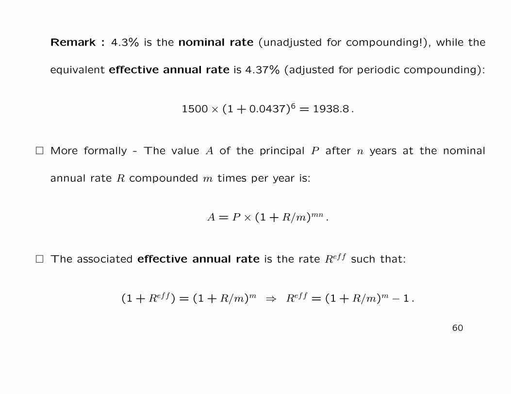
Remark : 4.3% is the nominal rate (unadjusted for compounding!), while the
equivalent effective annual rate is 4.37% (adjusted for periodic compounding):
1500× (1 + 0.0437)6 = 1938.8 .
� More formally - The value A of the principal P after n years at the nominal
annual rate R compounded m times per year is:
A = P × (1 +R/m)mn .
� The associated effective annual rate is the rate Reff such that:
(1 +Reff) = (1 +R/m)m ⇒ Reff = (1 +R/m)m − 1 .
60
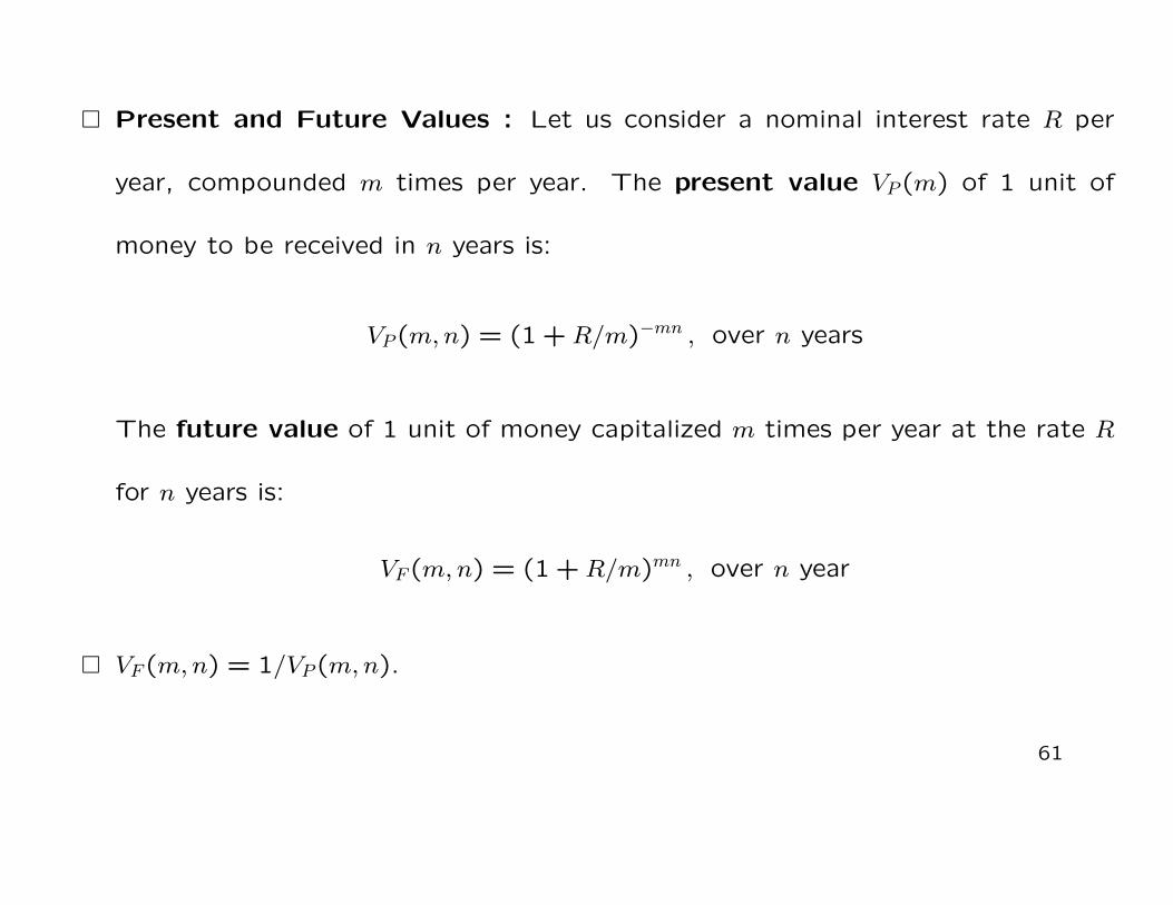
� Present and Future Values : Let us consider a nominal interest rate R per
year, compounded m times per year. The present value VP(m) of 1 unit of
money to be received in n years is:
VP(m,n) = (1 +R/m)−mn , over n years
The future value of 1 unit of money capitalized m times per year at the rate R
for n years is:
VF(m,n) = (1 +R/m)mn , over n year
� VF(m,n) = 1/VP(m,n).
61
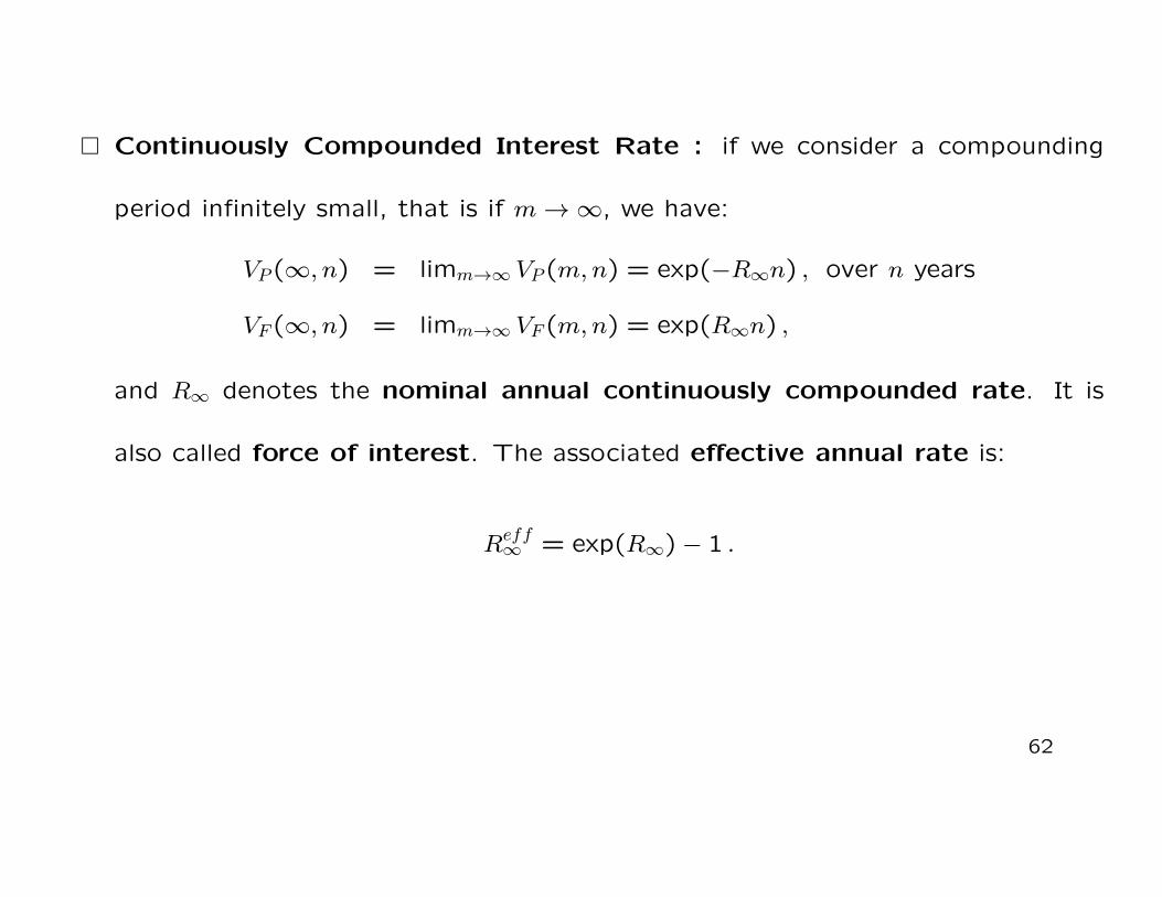
� Continuously Compounded Interest Rate : if we consider a compounding
period infinitely small, that is if m→∞, we have:
VP(∞, n) = limm→∞ VP(m,n) = exp(−R∞n) , over n years
VF(∞, n) = limm→∞ VF(m,n) = exp(R∞n) ,
and R∞ denotes the nominal annual continuously compounded rate. It is
also called force of interest. The associated effective annual rate is:
Reff∞ = exp(R∞)− 1 .
62
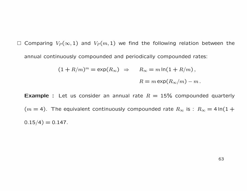
� Comparing VP(∞,1) and VP(m,1) we find the following relation between the
annual continuously compounded and periodically compounded rates:
(1 +R/m)m = exp(R∞) ⇒ R∞ = m ln(1 +R/m) ,
R = m exp(R∞/m)−m.
Example : Let us consider an annual rate R = 15% compounded quarterly
(m = 4). The equivalent continuously compounded rate R∞ is : R∞ = 4 ln(1 +
0.15/4) = 0.147.
63
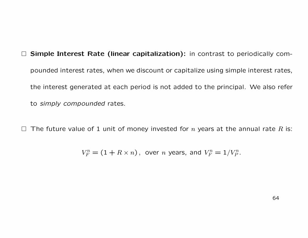
� Simple Interest Rate (linear capitalization): in contrast to periodically com-
pounded interest rates, when we discount or capitalize using simple interest rates,
the interest generated at each period is not added to the principal. We also refer
to simply compounded rates.
� The future value of 1 unit of money invested for n years at the annual rate R is:
V nF = (1 +R× n) , over n years, and V n
F = 1/V nP .
64
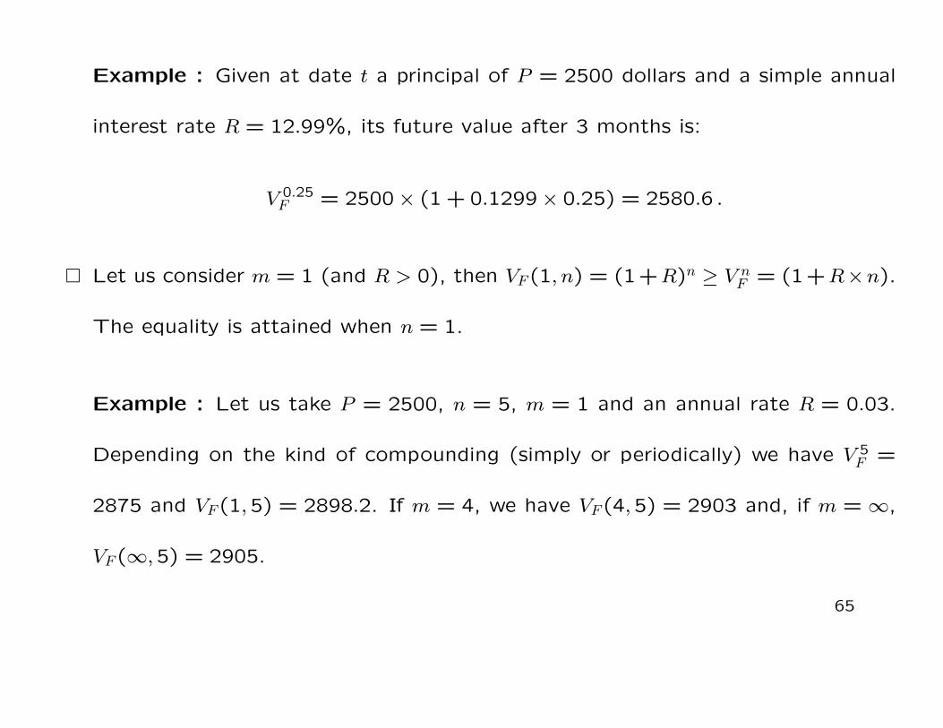
Example : Given at date t a principal of P = 2500 dollars and a simple annual
interest rate R = 12.99%, its future value after 3 months is:
V 0.25F = 2500× (1 + 0.1299× 0.25) = 2580.6 .
� Let us consider m = 1 (and R > 0), then VF(1, n) = (1 +R)n ≥ V nF = (1 +R×n).
The equality is attained when n = 1.
Example : Let us take P = 2500, n = 5, m = 1 and an annual rate R = 0.03.
Depending on the kind of compounding (simply or periodically) we have V 5F =
2875 and VF(1,5) = 2898.2. If m = 4, we have VF(4,5) = 2903 and, if m =∞,
VF(∞,5) = 2905.
65
1.3.2 Discount Factors: Bonds
• A zero-coupon bond (ZCB) is the simplest possible bond : it promises a single
and predetermined payment at the maturity date. This payment is called face
value, par value or principal. It is the amount of money paid to the bond holder
at the maturity date.
• A coupon bond is a bonds which promises, not only the face value at the
maturity date, but also other regular payments (coupons) between the date of
issue and the maturity date (included).
• The face value will be assumed (in general) equal to 1 unit of money (dollar).
66

• Let us denote by B(t, T ) the market value at the date t (date of potential issue)
of a zero-coupon bond, with unitary face value, maturing at date T (the maturity
date).
• The market price B(t, T ) represent the value at t for a ”sure” payment at T of
1 unit of money ⇒ B(t, T ) reflects the market Discount Factor of sure date T
payments.
• Indeed, if the ZCB face value at T is CT (say), then its price at t is CTB(t, T ):
the sure payment at T is discounted (actualized) at t by the Discount Factor
B(t, T ).
67
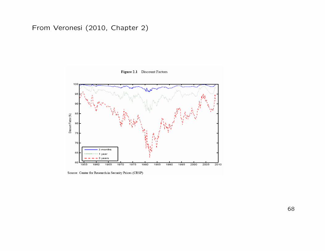
From Veronesi (2010, Chapter 2)
68
• If at the date t, several ZCBs with different maturity dates are traded, we can
form the function T → B(t, T ), called market Discount Function prevailing at
t.
• It is obvious that B(t, t) = 1 and B(t, S) < B(t, T ), ∀S > T . More precisely, the
discount function should be decreasing in the maturity date :
0 < B(t, S) < B(t, T ) < 1, S > T .
• A coupon bond has multiple payment dates Ti, {1, . . . , n}, T1 < . . . < Tn (with
Tn = T the maturity date). The payment (coupon) at date Ti is given (in general)
by the coupon rate ci times the face value CT . At T , the holder receives also CT .
69
• In general, payments occur at regular intervals (6 months for T-bills, T-bonds)
so that, for all i, Ti+1 − Ti = ∆i = ∆ for some fixed time interval ∆. If we
measure time in ”years”, typical bonds have ∆ ∈ {0.25,0.5,1} corresponding to
quarterly, semi-annual or annual payments.
• In many cases coupon rates ci are quoted as an annual rate even if they are paid
more frequently ⇒ the periodic coupon rate is ci∆.
• Let us consider the (classical) so-called bullet bonds or straight-coupon bonds :
here, all payments before the maturity date (Ti, i < n) are given by the product
of the coupon rate (ci) and the face value (CT). The payment at the maturity
date Tn = T is the sum of the coupon plus the face value.
70
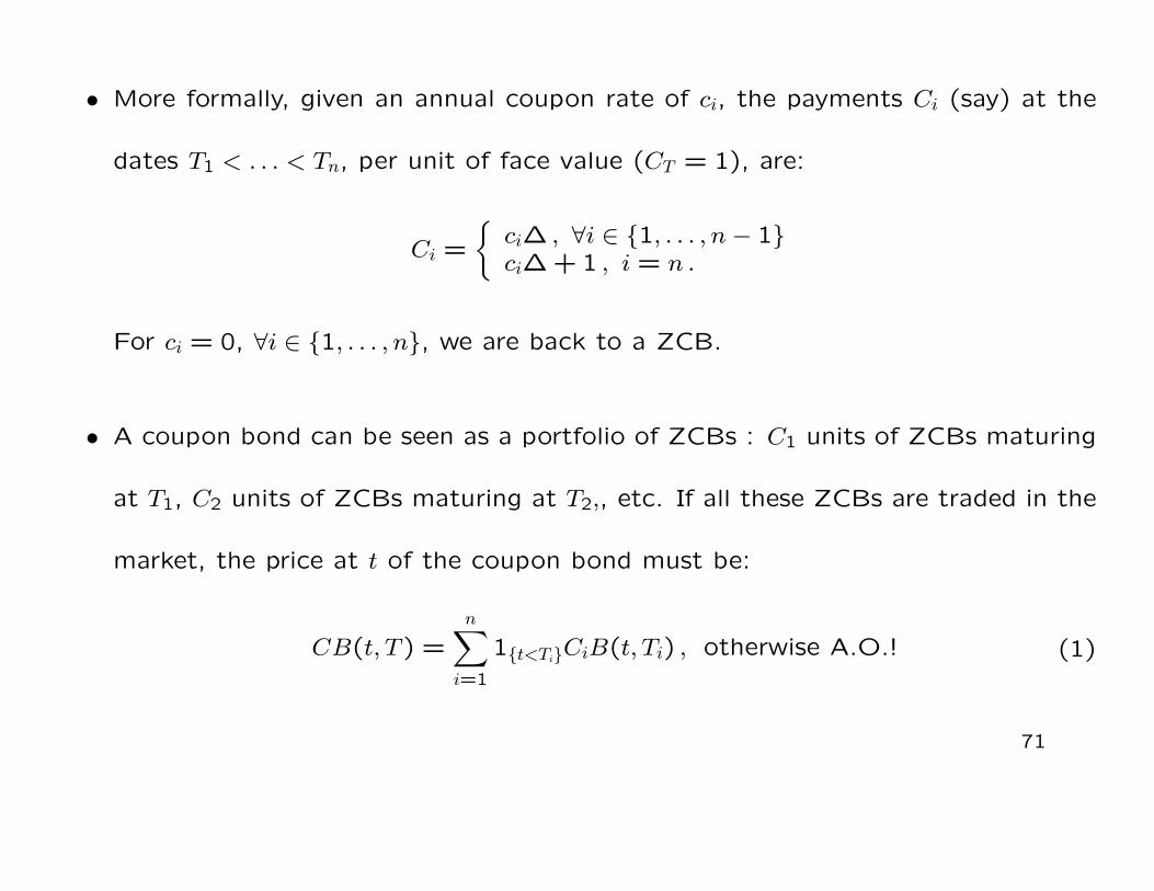
• More formally, given an annual coupon rate of ci, the payments Ci (say) at the
dates T1 < . . . < Tn, per unit of face value (CT = 1), are:
Ci =
{ci∆ , ∀i ∈ {1, . . . , n− 1}ci∆ + 1 , i = n .
For ci = 0, ∀i ∈ {1, . . . , n}, we are back to a ZCB.
• A coupon bond can be seen as a portfolio of ZCBs : C1 units of ZCBs maturing
at T1, C2 units of ZCBs maturing at T2,, etc. If all these ZCBs are traded in the
market, the price at t of the coupon bond must be:
CB(t, T ) =n∑i=1
1{t<Ti}CiB(t, Ti) , otherwise A.O.! (1)
71

• Example : Let us consider at date t, a bullet bond with CT = 100, an annual
coupon rate of 7% and time-to-maturity 3 years (T −t = 3 years). Suppose that,
at date t, ZCBs with face value equal to 1 dollar, are traded with residual maturity
of 1, 2 and 3 years. Assume that the market prices are B(t, t + 1y) = 0.98,
B(t, t + 2y) = 0.94 and B(t, t + 3y) = 0.90. The price of the bullet bond must
be:
CB(t, t+ 3y) = (0.07 · 100) · 0.98 + (0.07 · 100) · 0.94
+[(0.07 · 100) + 100] · 0.90 = 109.74.
↪→ if CB(t, t+3y) < 109.74 ⇒ the market provide an arbitrage opportunity, that is
a risk-free profit : at date t sell 7 one-year, 7 two-year and 107 three-year ZCBs
(earning 109.74), and buy the bullet bond at the market price CB(t, t+ 3y).
72
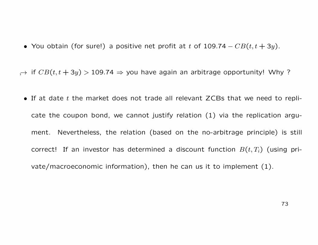
• You obtain (for sure!) a positive net profit at t of 109.74− CB(t, t+ 3y).
↪→ if CB(t, t+ 3y) > 109.74 ⇒ you have again an arbitrage opportunity! Why ?
• If at date t the market does not trade all relevant ZCBs that we need to repli-
cate the coupon bond, we cannot justify relation (1) via the replication argu-
ment. Nevertheless, the relation (based on the no-arbitrage principle) is still
correct! If an investor has determined a discount function B(t, Ti) (using pri-
vate/macroeconomic information), then he can us it to implement (1).
73
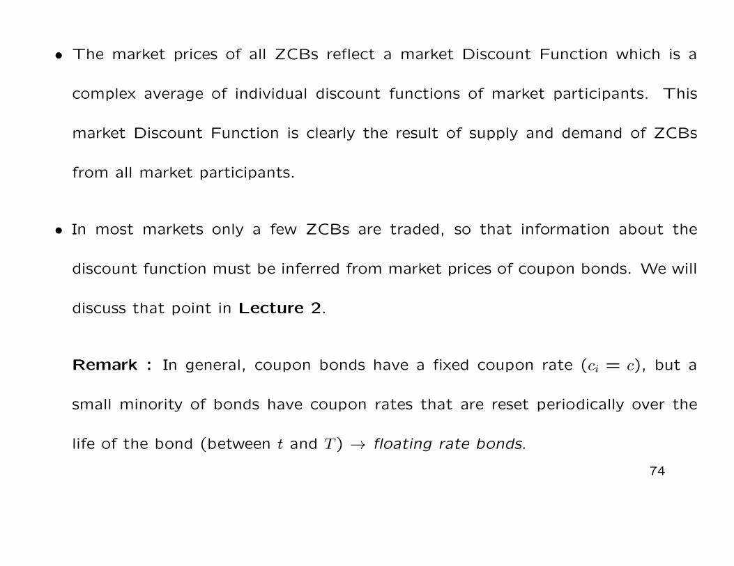
• The market prices of all ZCBs reflect a market Discount Function which is a
complex average of individual discount functions of market participants. This
market Discount Function is clearly the result of supply and demand of ZCBs
from all market participants.
• In most markets only a few ZCBs are traded, so that information about the
discount function must be inferred from market prices of coupon bonds. We will
discuss that point in Lecture 2.
Remark : In general, coupon bonds have a fixed coupon rate (ci = c), but a
small minority of bonds have coupon rates that are reset periodically over the
life of the bond (between t and T ) → floating rate bonds.
74
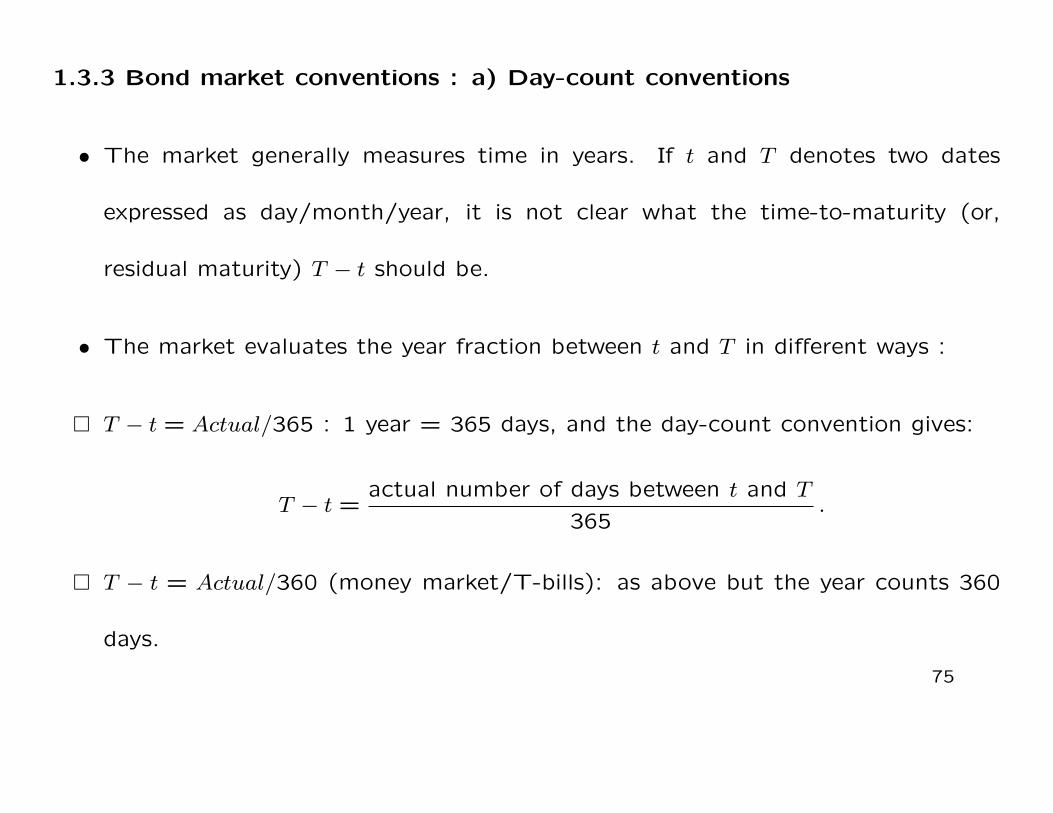
1.3.3 Bond market conventions : a) Day-count conventions
• The market generally measures time in years. If t and T denotes two dates
expressed as day/month/year, it is not clear what the time-to-maturity (or,
residual maturity) T − t should be.
• The market evaluates the year fraction between t and T in different ways :
� T − t = Actual/365 : 1 year = 365 days, and the day-count convention gives:
T − t =actual number of days between t and T
365.
� T − t = Actual/360 (money market/T-bills): as above but the year counts 360
days.
75
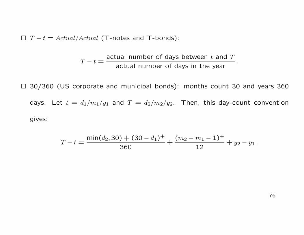
� T − t = Actual/Actual (T-notes and T-bonds):
T − t =actual number of days between t and T
actual number of days in the year.
� 30/360 (US corporate and municipal bonds): months count 30 and years 360
days. Let t = d1/m1/y1 and T = d2/m2/y2. Then, this day-count convention
gives:
T − t =min(d2,30) + (30− d1)+
360+
(m2 −m1 − 1)+
12+ y2 − y1 .
76
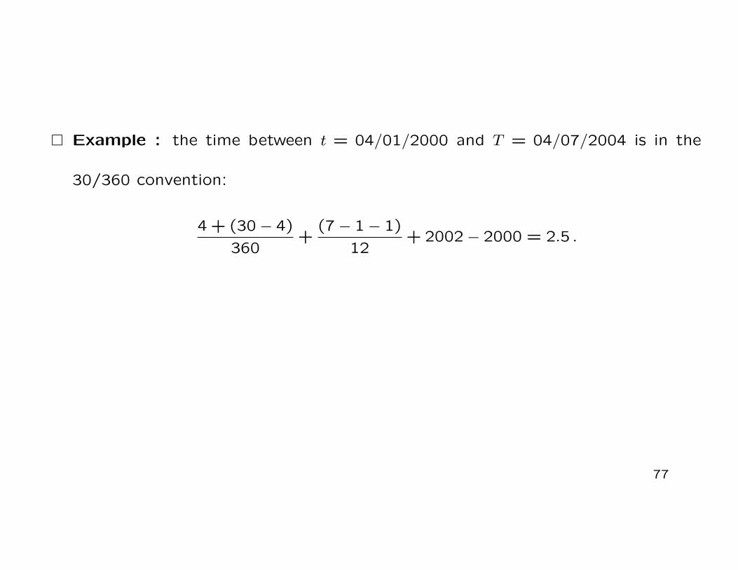
� Example : the time between t = 04/01/2000 and T = 04/07/2004 is in the
30/360 convention:
4 + (30− 4)
360+
(7− 1− 1)
12+ 2002− 2000 = 2.5 .
77
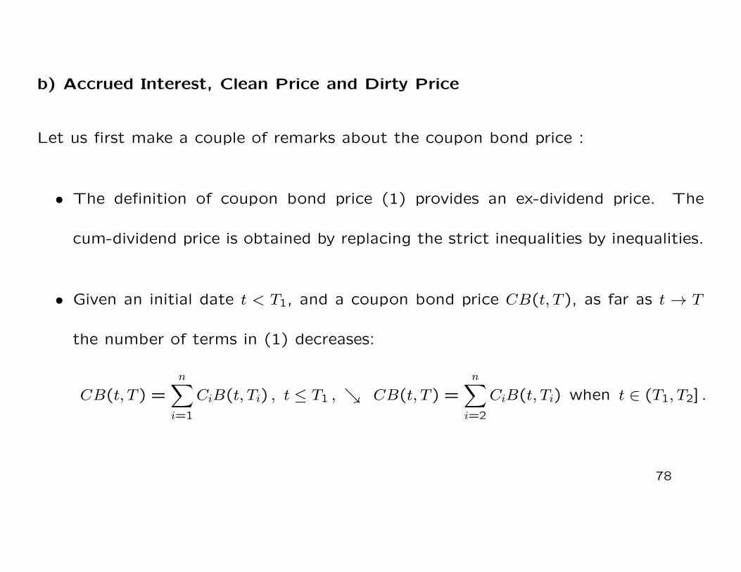
b) Accrued Interest, Clean Price and Dirty Price
Let us first make a couple of remarks about the coupon bond price :
• The definition of coupon bond price (1) provides an ex-dividend price. The
cum-dividend price is obtained by replacing the strict inequalities by inequalities.
• Given an initial date t < T1, and a coupon bond price CB(t, T ), as far as t → T
the number of terms in (1) decreases:
CB(t, T ) =n∑i=1
CiB(t, Ti) , t ≤ T1 , ↘ CB(t, T ) =n∑i=2
CiB(t, Ti) when t ∈ (T1, T2] .
78
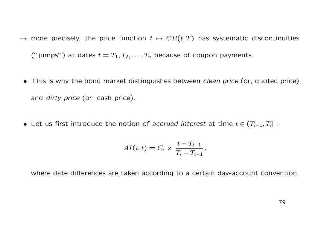
→ more precisely, the price function t 7→ CB(t, T ) has systematic discontinuities
(”jumps”) at dates t = T1, T2, . . . , Tn because of coupon payments.
• This is why the bond market distinguishes between clean price (or, quoted price)
and dirty price (or, cash price).
• Let us first introduce the notion of accrued interest at time t ∈ (Ti−1, Ti] :
AI(i; t) = Ci ×t− Ti−1
Ti − Ti−1,
where date differences are taken according to a certain day-account convention.
79

• The clean price at date t of the coupon bond is
CBclean(t, T ) = CB(t, T )−AI(i; t) , t ∈ (Ti−1, Ti] .
• In other words, when we buy a coupon bond quoted at the clean price CBclean(t, T )
at date t ∈ (Ti−1, Ti], the cash price we have to pay is:
CB(t, T ) = CBclean(t, T ) +AI(i; t) , t ∈ (Ti−1, Ti] .
80
1.3.4 Bond yields and zero-coupon rates
• Even if discount factors (B(t, T )) provide full information about how to discount
future sure payments, it is much easier to interpret (and compare) the information
provided by interest rates (a given percentage per year).
• Nevertheless, to correctly use and assess the magnitude of an interest rate, we
need to know the compounding frequency of that rate.
• Moreover, it is important to know at which time the rate is set or observed,
and over which period of time the interest rate applies.
81
• Here, we will introduce spot rates (they apply to a period beginning at the time
the rate is set), and then we will present forward rates (they apply to a period
beginning after the date they set).
� Yield of a coupon bond - Given at date t a coupon bond with maturity date
T , price CB(t, T ) and payments {C1, . . . , Cn} at dates {T1, . . . , Tn}, respectively,
the associated annually compounded yield to maturity is the value Y CB(t, T )
satisfying the equation:
CB(t, T ) =n∑i=1
Ci(1 + Y CB(t, T ))−(Ti−t) .
Note that the same discount rate is applied to all payments!
82

� Yield of a ZCB with CT = 1 at the maturity date T - The annually com-
pounded yield to maturity (m = 1) is the value Y (t, T ) satisfying the equation:
B(t, T ) = (1 + Y (t, T ))−(T−t) ,
and therefore we have Y (t, T ) = B(t, T )−1/(T−t) − 1;
→ we call Y (t, T ) the annually compounded zero-coupon yield, or zero-coupon
rate, or spot rate for date T .
→ the function T 7→ Y (t, T ) is called the (annually compounded) zero-coupon yield
curve or simply the yield curve. It provides the same information as T 7→ B(t, T ).
83
� The continuously compounded yield to maturity of the above mentioned
coupon bond is the value RCB(t, T ) (also called gross redemption yield) satisfying
the equation:
CB(t, T ) =n∑i=1
Ci exp[−RCB(t, T )× (Ti − t)] .
� The quoted YTM RCB(t, T ) (say) is the periodically compounded rate with cap-
italization frequency (m) equal to the coupon frequency:
RCB(t, T ) = m exp[RCB(t, T )/m]−m.
Example : If the coupons are semiannual (m = 2), then
RCB(t, T ) = 2[exp[RCB(t, T )/2]− 1].
84

� The function T 7→ RCB(t, T ) is also a yield curve providing the same information
as T 7→ CB(t, T ) or T 7→ Y CB(t, T ).
� In the particular case of a ZCB, the continuously compounded yield to ma-
turity R(t, T ) satisfies:
B(t, T ) = exp[−R(t, T )× (T − t)] , ⇒ R(t, T ) = −1
T − tlnB(t, T ) . (2)
� R(t, T ) = ln(1 + Y (t, T )), is also called the term structure of interest rates.
� There is an inverse relation between yield and associated bond price level.
� For mathematical convenience we will focus on R(t, T ) in most models.
85
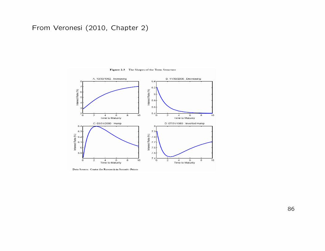
From Veronesi (2010, Chapter 2)
86
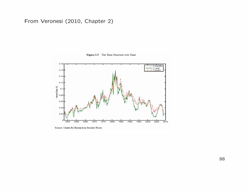
From Veronesi (2010, Chapter 2)
87
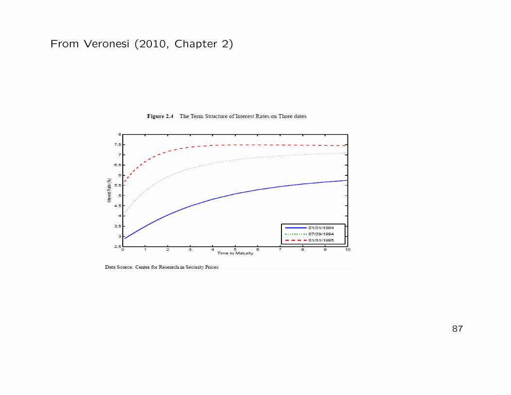
From Veronesi (2010, Chapter 2)
88

Example : Let us assume that at date t we observe on the zero-coupon bond
market the following continuously compounded yield curve (annual basis!) :
T − t 0.5 1 1.5 2
R(t, T ) 2.5% 2.0% 2.7% 3.0%
Q : Which is the price at date t of the coupon bond with residual maturity 2 years,
CT = 100, semiannual coupons with annual coupon rate of 7% and coupon dates
T1 = t+ 0.5, T2 = t+ 1, T3 = t+ 1.5 and T4 = t+ 2? Determine its continuously
compounded YTM and its quoted YTM.
89

A.1 : First, we determine the zero-coupon bond prices :
B(t, t+ 0.5) = exp[−0.025× 0.5] = 0.9876
B(t, t+ 1) = exp[−0.02] = 0.9802
B(t, t+ 1.5) = exp[−0.027× 1.5] = 0.9603
B(t, t+ 2) = exp[−0.03× 2] = 0.9418 .
⇒ the coupon bond price is:
CB(t, t+ 2) = 3.5× [B(t, t+ 0.5) +B(t, t+ 1) +B(t, t+ 1.5)]
+103.5×B(t, t+ 2)
= 3.5× [0.9876 + 0.9802 + 0.9603] + 103.5× 0.9418
= 107.7246 .
90

A.2 : The associated continuously compounded YTM is the rate RCB(t, t + 2) such
that:
CB(t, t+ 2) = 107.7246 = 3.5× [e−0.5RCB(t,t+2) + e−RCB(t,t+2) + e−1.5RCB(t,t+2)]
+103.5× e−2RCB(t,t+2) ,
⇒ RCB(t, t+ 2) = 2.97% .
A.3 : The quoted YTM, with semiannual coupons, is:
RCB(t, t+ 2) = 2(eRCB(t,t+2)/2 − 1) = 2.999% .
91
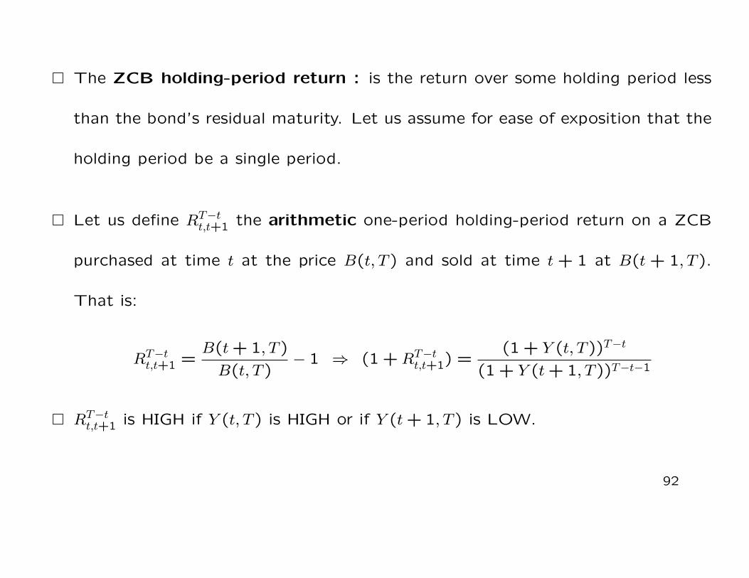
� The ZCB holding-period return : is the return over some holding period less
than the bond’s residual maturity. Let us assume for ease of exposition that the
holding period be a single period.
� Let us define RT−tt,t+1 the arithmetic one-period holding-period return on a ZCB
purchased at time t at the price B(t, T ) and sold at time t + 1 at B(t + 1, T ).
That is:
RT−tt,t+1 =
B(t+ 1, T )
B(t, T )− 1 ⇒ (1 +RT−t
t,t+1) =(1 + Y (t, T ))T−t
(1 + Y (t+ 1, T ))T−t−1
� RT−tt,t+1 is HIGH if Y (t, T ) is HIGH or if Y (t+ 1, T ) is LOW.
92
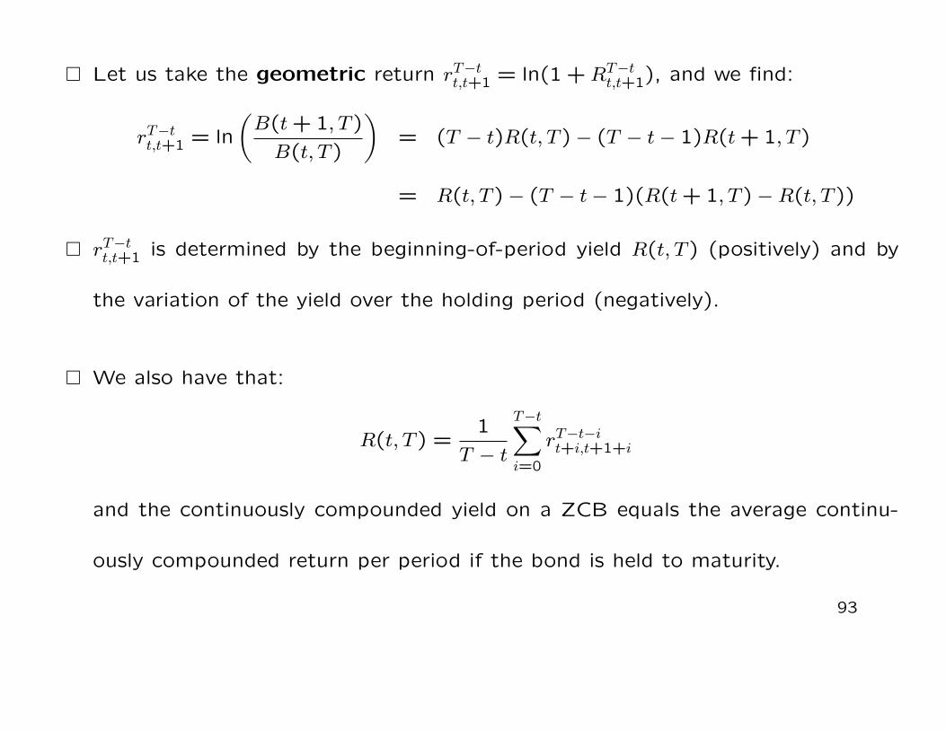
� Let us take the geometric return rT−tt,t+1 = ln(1 +RT−tt,t+1), and we find:
rT−tt,t+1 = ln
(B(t+ 1, T )
B(t, T )
)= (T − t)R(t, T )− (T − t− 1)R(t+ 1, T )
= R(t, T )− (T − t− 1)(R(t+ 1, T )−R(t, T ))
� rT−tt,t+1 is determined by the beginning-of-period yield R(t, T ) (positively) and by
the variation of the yield over the holding period (negatively).
� We also have that:
R(t, T ) =1
T − t
T−t∑i=0
rT−t−it+i,t+1+i
and the continuously compounded yield on a ZCB equals the average continu-
ously compounded return per period if the bond is held to maturity.
93

� Spot LIBOR rate : the simply compounded interest rate convention is typically
applied for commercial loans (fixed and floating reference rate loans). The most
commonly used floating reference rate is the LIBOR (London Interbank Offered
Rate).
� Let us consider, at date t, the quoted LIBOR annual rate with maturity date T ,
denoted L(t, T ) (say). The present value of 1 unit of money paid at T is:
BL(t, T ) =1
[1 + L(t, T )× (T − t)],
that is:
L(t, T ) =1
T − t
(1
BL(t, T )− 1
),
94

� If in the market we have at date t a ZCB maturing at T with price B(t, T ), for
arbitrage reasons we must have BL(t, T ) = B(t, T ). Indeed, let us imagine that,
at time t, we have BL(t, T ) > B(t, T ). In that case, an investor can make a sure
positive profit.
→ He borrows at t, over the period [t, T ], the amount of money BL(t, T ) at the
simple rate L(t, T ) and he buys (again, at t) the ZCB paying the price B(t, T ).
⇒ At t he earns BL(t, T ) − B(t, T ), while at T he has a null profit : he obtain 1
unit of money from the ZCB and he provide the amount of money BL(t, T )[1 +
L(t, T )× (T − t)] = 1.
95
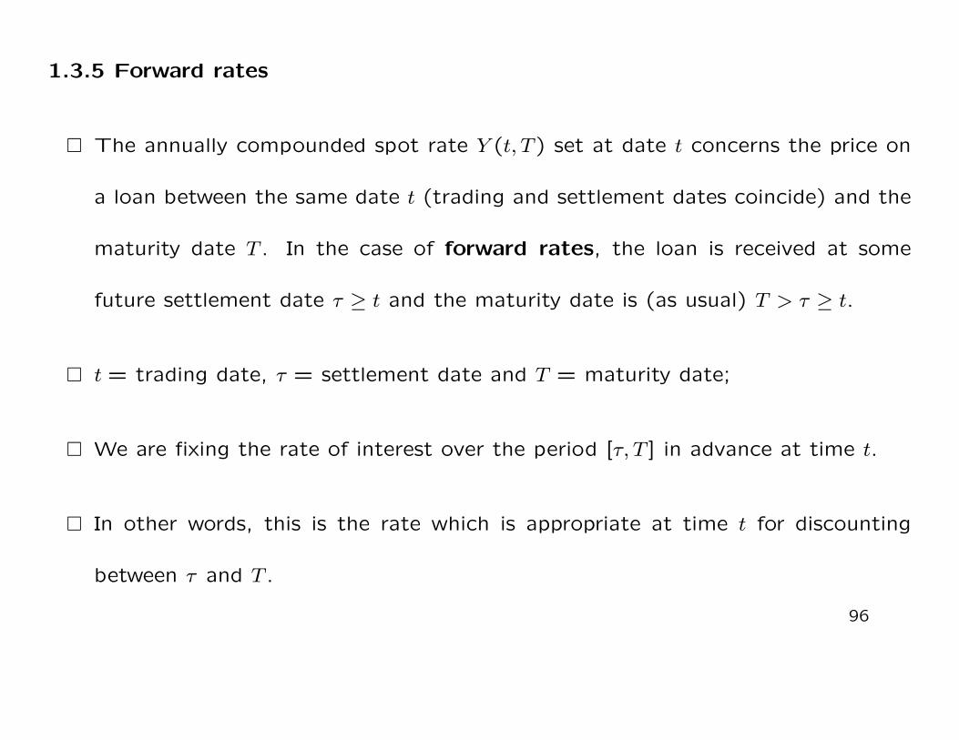
1.3.5 Forward rates
� The annually compounded spot rate Y (t, T ) set at date t concerns the price on
a loan between the same date t (trading and settlement dates coincide) and the
maturity date T . In the case of forward rates, the loan is received at some
future settlement date τ ≥ t and the maturity date is (as usual) T > τ ≥ t.
� t = trading date, τ = settlement date and T = maturity date;
� We are fixing the rate of interest over the period [τ, T ] in advance at time t.
� In other words, this is the rate which is appropriate at time t for discounting
between τ and T .
96
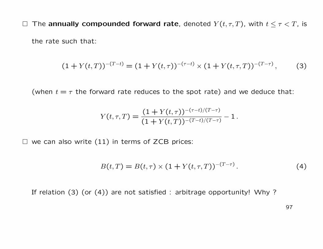
� The annually compounded forward rate, denoted Y (t, τ, T ), with t ≤ τ < T , is
the rate such that:
(1 + Y (t, T ))−(T−t) = (1 + Y (t, τ))−(τ−t) × (1 + Y (t, τ, T ))−(T−τ) , (3)
(when t = τ the forward rate reduces to the spot rate) and we deduce that:
Y (t, τ, T ) =(1 + Y (t, τ))−(τ−t)/(T−τ)
(1 + Y (t, T ))−(T−t)/(T−τ)− 1 .
� we can also write (11) in terms of ZCB prices:
B(t, T ) = B(t, τ)× (1 + Y (t, τ, T ))−(T−τ) . (4)
If relation (3) (or (4)) are not satisfied : arbitrage opportunity! Why ?
97

� The short (annually compounded) forward rate is given by:
Y (t, τ, τ + 1) =B(t, τ)
B(t, τ + 1)− 1 .
� This means that we can define the following relation between the zero-coupon
bond price and the sequence of short forward rates applying over time-to-maturity
interval:
B(t, τ) =τ−1∏j=t
B(t, j + 1)
B(t, j)=
τ−1∏j=t
1
1 + Y (t, j, j + 1).
98

� The forward LIBOR rate at date t, valid for the period [τ, T ], is the simply
compounded rate L(t, τ, T ) such that:
B(t, τ) = B(t, T )× [1 + L(t, τ, T )× (T − τ)] , (5)
and therefore
L(t, τ, T ) =1
T − τ
(B(t, τ)
B(t, T )− 1
).
� The continuously compounded forward rate prevailing at date t, for the period
[τ, T ], is the rate R(t, τ, T ) such that:
exp[−R(t, T )× (T − t)] = exp[−R(t, τ)× (τ − t)]× exp[−R(t, τ, T )× (T − τ)] .
99

� This means that R(t, τ, T ) is given by:
R(t, τ, T ) = −1
T − τlnB(t, T )
B(t, τ),
=R(t, T )(T − t)−R(t, τ)(τ − t)
T − τ.
(6)
� the quantity R(t, τ, τ + 1) = ln B(t,τ)B(t,τ+1)
is called the short forward rate and gives
the possibility to write:
B(t, τ) = exp[−∑τ−1
j=t R(t, j, j + 1)]. (7)
100
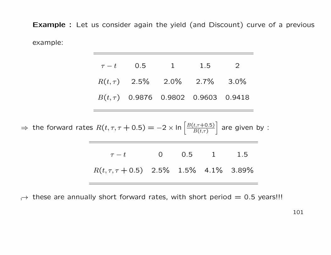
Example : Let us consider again the yield (and Discount) curve of a previous
example:
τ − t 0.5 1 1.5 2
R(t, τ) 2.5% 2.0% 2.7% 3.0%
B(t, τ) 0.9876 0.9802 0.9603 0.9418
⇒ the forward rates R(t, τ, τ + 0.5) = −2× ln[B(t,τ+0.5)B(t,τ)
]are given by :
τ − t 0 0.5 1 1.5
R(t, τ, τ + 0.5) 2.5% 1.5% 4.1% 3.89%
↪→ these are annually short forward rates, with short period = 0.5 years!!!
101

⇒ we can also apply formula (7), using the above determined short forward rates,
to find again the zero-coupon bond prices:
B(t, t+ 0.5) = exp[−0.025× 0.5] = 0.9876
B(t, t+ 1) = exp[−0.5× (0.025 + 0.015)] = 0.9802
B(t, t+ 1.5) = exp[−0.5× (0.025 + 0.015 + 0.041)] = 0.9603
B(t, t+ 2) = exp[−0.5× (0.025 + 0.015 + 0.041 + 0.0389)] = 0.9418 .
Remark : Observe that we have to convert annual short forward rates on a
semiannual basis, given that the time step is the semester.
102

� Frequently, in the asset pricing literature we focus on forward rates for future
periods of infinitesimal length. The so-called instantaneous forward rate is
defined as:
f(t, τ) = limT→τ R(t, τ, T ) ,
and the function τ 7→ f(t, τ) is called the term structure of instantaneous
forward rates or the instantaneous forward rate curve.
� Letting T → τ in relation (13) we get by definition:
f(t, τ) = −∂ lnB(t, τ)
∂τ= −
∂B(t, τ)/∂τ
B(t, τ), (8)
assuming a differentiable discounting function B(t, τ).
103
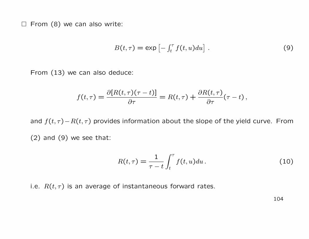
� From (8) we can also write:
B(t, τ) = exp[−∫ τtf(t, u)du
]. (9)
From (13) we can also deduce:
f(t, τ) =∂[R(t, τ)(τ − t)]
∂τ= R(t, τ) +
∂R(t, τ)
∂τ(τ − t) ,
and f(t, τ)−R(t, τ) provides information about the slope of the yield curve. From
(2) and (9) we see that:
R(t, τ) =1
τ − t
∫ τ
t
f(t, u)du . (10)
i.e. R(t, τ) is an average of instantaneous forward rates.
104

� R(t, T ) can be seen as a risk-free rate of return, over the fixed period [t, T ],
induce by the investment in B(t, T ). In the continuous time literature, when we
talk about the risk-free rate, or the short rate we mean the instantaneous
spot rate defined as:
r(t) = limT→t+ R(t, T ) = limT→t+ f(t, T ) .
� The short rate r(t) gives the possibility to introduce the notion of bank ac-
count: this (instantaneously) risk-free asset is a continuous roll-over of such
instantaneously risk-free investments. Let A = (At) denote the price process of
the bank account.
105
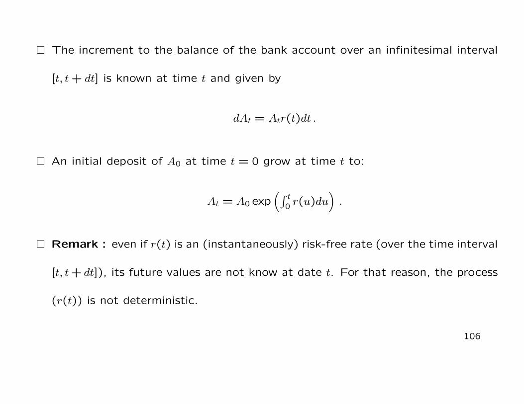
� The increment to the balance of the bank account over an infinitesimal interval
[t, t+ dt] is known at time t and given by
dAt = Atr(t)dt .
� An initial deposit of A0 at time t = 0 grow at time t to:
At = A0 exp(∫ t
0 r(u)du).
� Remark : even if r(t) is an (instantaneously) risk-free rate (over the time interval
[t, t+ dt]), its future values are not know at date t. For that reason, the process
(r(t)) is not deterministic.
106
1.3.6 Forward Rates and Forward Discount Factors
� We have seen that the annually compounded spot rate Y (t, T ) set at date t
concerns the price on a loan between the same date t (trading and settlement
dates coincide) and the maturity date T .
� In the case of forward rates, the loan is received at some future settlement
date τ ≥ t and the maturity date is (as usual) T > τ ≥ t (t = trading date, τ =
settlement date and T = maturity date).
� In other words, this is the rate which is appropriate at time t for discounting
between τ and T .
107

� The annually compounded forward rate, denoted Y (t, τ, T ), with t ≤ τ < T , is
the rate such that:
(1 + Y (t, T ))−(T−t) = (1 + Y (t, τ))−(τ−t) × (1 + Y (t, τ, T ))−(T−τ) , (11)
(when t = τ the forward rate reduces to the spot rate). We can also write (11)
in terms of forward discount factor F (t, τ, T ):
F (t, τ, T ) =B(t, T )
B(t, τ)=
1
(1 + Y (t, τ, T ))(T−τ). (12)
� The forward discount factor at time t defines the time value of money between
two future dates, τ and T > τ , and it is given by the ratio of the two date-t
discount factors B(t, τ) and B(t, T ).
108

� The forward discount factor has the following properties: i) F (t, τ, T ) = 1 for
T = τ ; ii) F (t, τ, T ) is decreasing in T .
� The forward rate at time t for a risk-free investment from τ to T , and with
compounding frequency m, is the interest rate determined by F (t, τ, T ):
Y (m)(t, τ, T ) = m ×
1
F (t, τ, T )
1
m (T − τ)
− 1
.
� The continuously compounded forward rate is obtained for m→ +∞:
R(t, τ, T ) = −1
(T − τ)ln(F (t, τ, T )) .
109
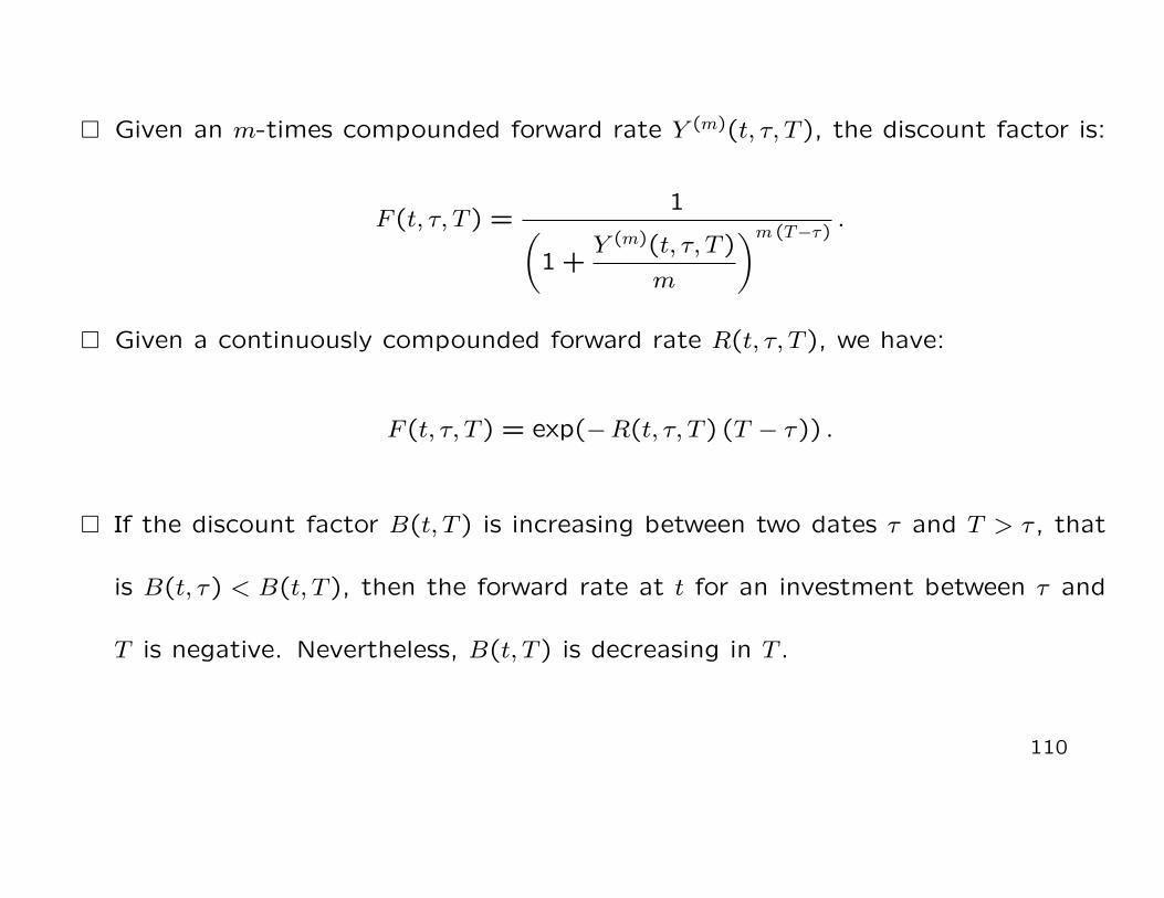
� Given an m-times compounded forward rate Y (m)(t, τ, T ), the discount factor is:
F (t, τ, T ) =1(
1 +Y (m)(t, τ, T )
m
)m (T−τ).
� Given a continuously compounded forward rate R(t, τ, T ), we have:
F (t, τ, T ) = exp(−R(t, τ, T ) (T − τ)) .
� If the discount factor B(t, T ) is increasing between two dates τ and T > τ , that
is B(t, τ) < B(t, T ), then the forward rate at t for an investment between τ and
T is negative. Nevertheless, B(t, T ) is decreasing in T .
110
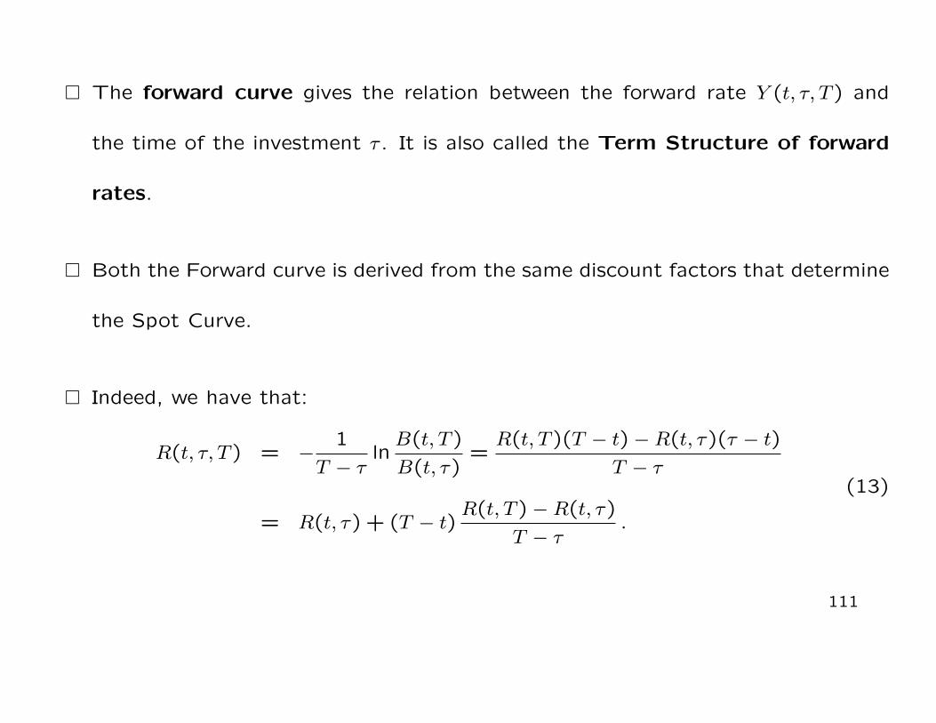
� The forward curve gives the relation between the forward rate Y (t, τ, T ) and
the time of the investment τ . It is also called the Term Structure of forward
rates.
� Both the Forward curve is derived from the same discount factors that determine
the Spot Curve.
� Indeed, we have that:
R(t, τ, T ) = −1
T − τlnB(t, T )
B(t, τ)=R(t, T )(T − t)−R(t, τ)(τ − t)
T − τ
= R(t, τ) + (T − t)R(t, T )−R(t, τ)
T − τ.
(13)
111
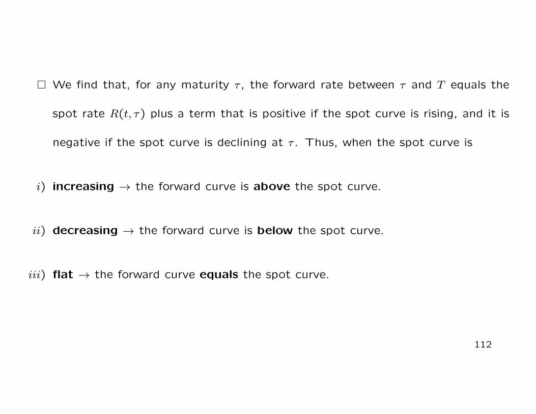
� We find that, for any maturity τ , the forward rate between τ and T equals the
spot rate R(t, τ) plus a term that is positive if the spot curve is rising, and it is
negative if the spot curve is declining at τ . Thus, when the spot curve is
i) increasing → the forward curve is above the spot curve.
ii) decreasing → the forward curve is below the spot curve.
iii) flat → the forward curve equals the spot curve.
112

2,5
3
3,5
4
4,5
5
Inte
rest
Ra
tes
(an
nu
al
ba
sis)
Svensson forward and spot curves
Forward curve
Spot curve
Term Structure of
Spot Rates
0
0,5
1
1,5
2
1 6 11 16 21 26 31 36
Inte
rest
Ra
tes
(an
nu
al
ba
sis)
Spot curve
Term Structure of
Forward Rates
113
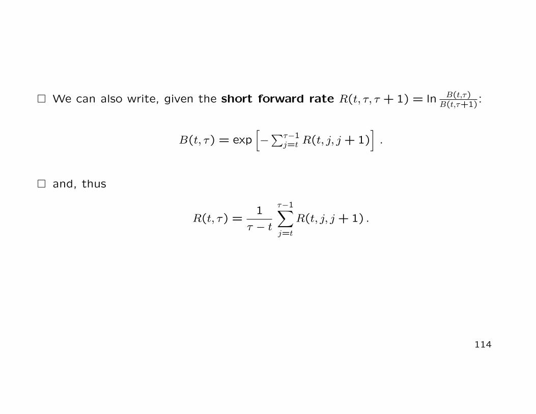
� We can also write, given the short forward rate R(t, τ, τ + 1) = ln B(t,τ)B(t,τ+1)
:
B(t, τ) = exp[−∑τ−1
j=t R(t, j, j + 1)].
� and, thus
R(t, τ) =1
τ − t
τ−1∑j=t
R(t, j, j + 1) .
114

� We have also seen that the simply compounded forward (LIBOR) rate at
date t, valid for the period [τ, T ], is the rate L(t, τ, T ) such that:
B(t, τ) = B(t, T )× [1 + L(t, τ, T )× (T − τ)] .
� The simply compounded forward discount factor LF (t, τ, T ) is thus:
LF (t, τ, T ) =B(t, T )
B(t, τ)=
1
[1 + L(t, τ, T )× (T − τ)].
� and therefore
L(t, τ, T ) =1
T − τ
(B(t, τ)
B(t, T )− 1
).
115
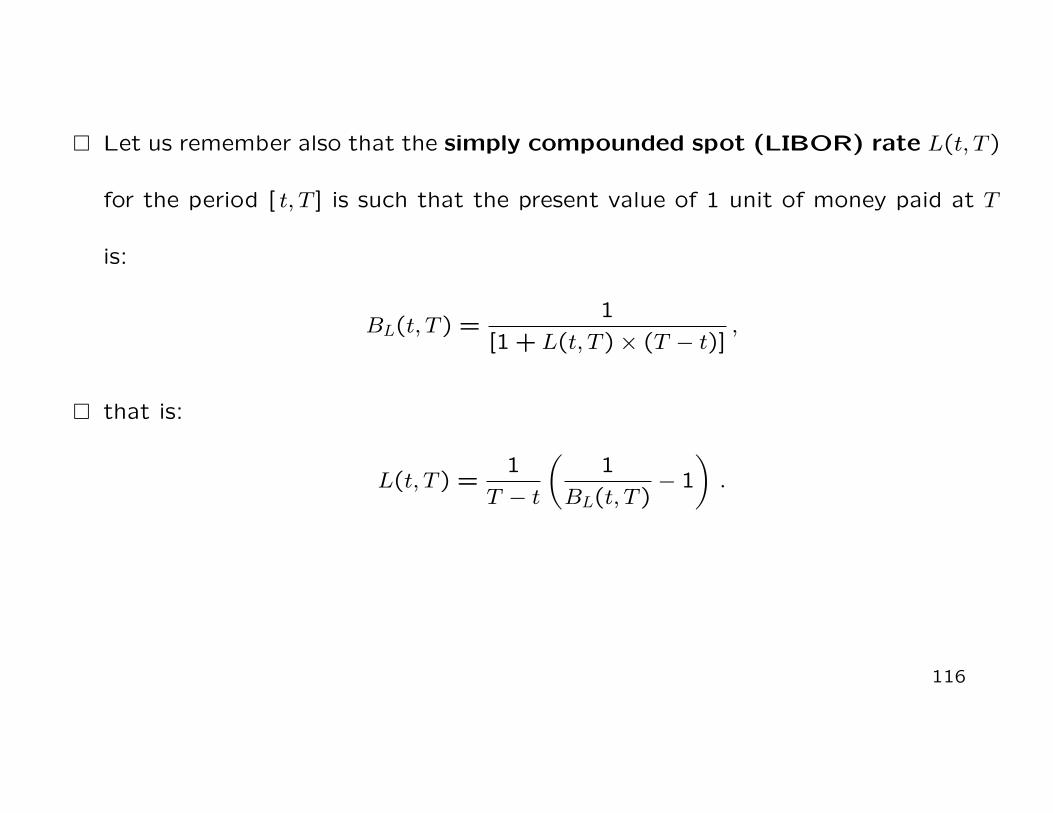
� Let us remember also that the simply compounded spot (LIBOR) rate L(t, T )
for the period [ t, T ] is such that the present value of 1 unit of money paid at T
is:
BL(t, T ) =1
[1 + L(t, T )× (T − t)],
� that is:
L(t, T ) =1
T − t
(1
BL(t, T )− 1
).
116
1.3.7 Par yields
� It is a popular way to express yields on coupon-bearing bonds is by means of the
concept of par yield.
� The par yield at date t for a given maturity date T , denoted ρ(t, T ) (say), is the
coupon rate of a bullet bond making its price at date t equal to its par (face)
value (CB(0, T ) = CT).
� Even if zero-coupon yields are a more fundamental concept, par yields remain
an alternative way to represent the yield curve. They are two alternative way to
represent the information in the discount function.
117
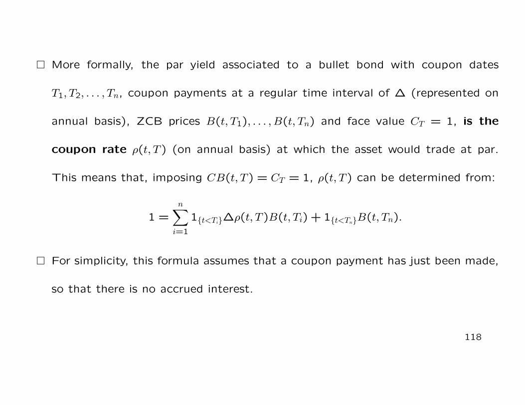
� More formally, the par yield associated to a bullet bond with coupon dates
T1, T2, . . . , Tn, coupon payments at a regular time interval of ∆ (represented on
annual basis), ZCB prices B(t, T1), . . . , B(t, Tn) and face value CT = 1, is the
coupon rate ρ(t, T ) (on annual basis) at which the asset would trade at par.
This means that, imposing CB(t, T ) = CT = 1, ρ(t, T ) can be determined from:
1 =n∑i=1
1{t<Ti}∆ρ(t, T )B(t, Ti) + 1{t<Tn}B(t, Tn).
� For simplicity, this formula assumes that a coupon payment has just been made,
so that there is no accrued interest.
118
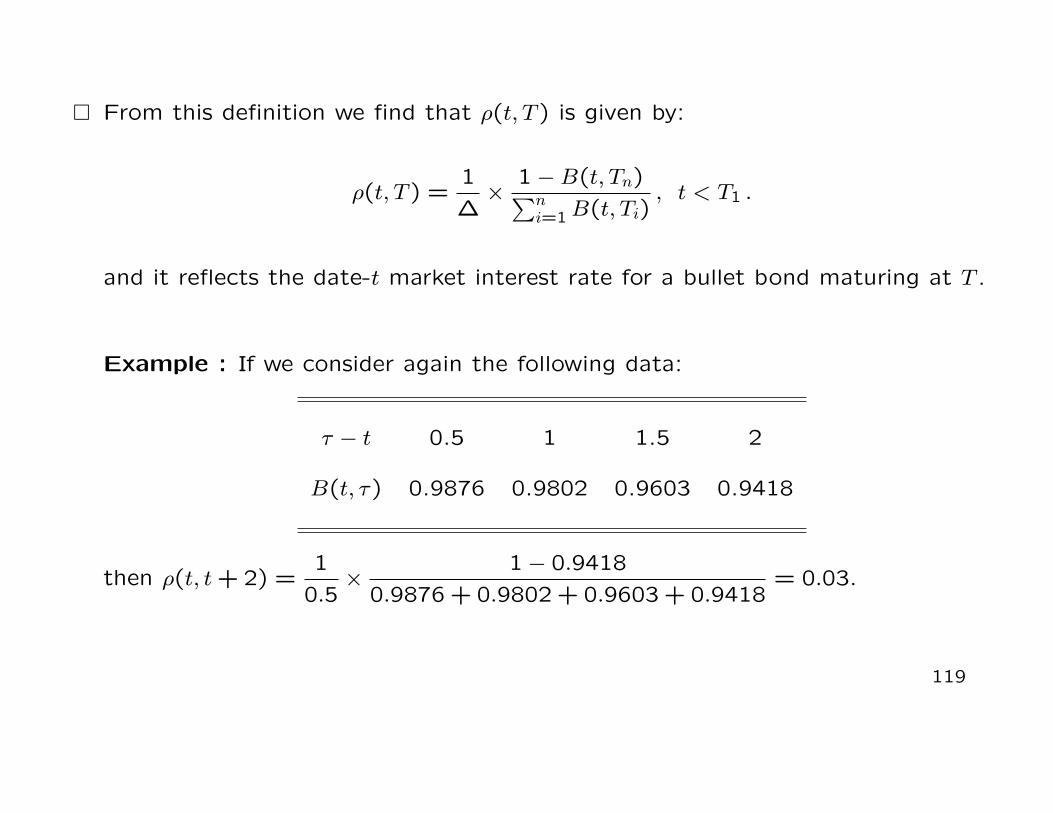
� From this definition we find that ρ(t, T ) is given by:
ρ(t, T ) =1
∆×
1−B(t, Tn)∑ni=1B(t, Ti)
, t < T1 .
and it reflects the date-t market interest rate for a bullet bond maturing at T .
Example : If we consider again the following data:
τ − t 0.5 1 1.5 2
B(t, τ) 0.9876 0.9802 0.9603 0.9418
then ρ(t, t+ 2) =1
0.5×
1− 0.9418
0.9876 + 0.9802 + 0.9603 + 0.9418= 0.03.
119
1.3.8 Inflation-Indexed Bonds
� In this course we will mainly focus on bonds paying coupons and the final principal
in dollars (say). In other words, the payments are fixed in nominal terms.
� Nevertheless, how much of a good an investor (a consumer) can buy with the
given amount of dollars, obtained from the coupon and principal payments,
depends on the inflation between the purchase of the bond and the coupon
and principal payments.
120

� The CPI index, computed monthly by the Bureau of Labor Statistics (BLS),
provides a weighted average of the value of a basket of representative goods
that U.S. consumers purchase.
� The are different measures of the CPI, depending on the location and the type
of goods considered. Here we consider the non-seasonally-adjusted U.S. City
Average All Items Consumer Price Index (CPI − U), which is the index used for
TIPS.
� The CPI variation over time measures the realized inflation (over that period)
and it identifies the inflation risk.
121
� Inflation risk is the loss of purchasing power of the dollar. All assets that provide
future payment in fixed nominal terms are affected by inflation risk.
� Let us show how are calculated the payments of inflation-linked bonds. We
will focus, in particular, on TIPS (Treasury Inflation Protected Securities) traded
in the U.S. bond market.
� TIPS are coupon bonds issued with maturities 5, 10 and 20 years. The coupon
rate of TIPS is a constant fraction of the principal but the principal is not fixed:
it changes over time to compensate for inflation.
122
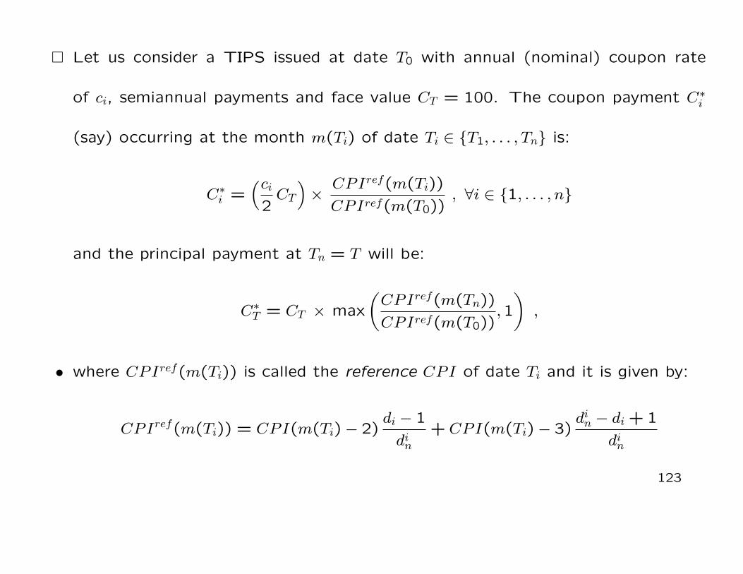
� Let us consider a TIPS issued at date T0 with annual (nominal) coupon rate
of ci, semiannual payments and face value CT = 100. The coupon payment C∗i
(say) occurring at the month m(Ti) of date Ti ∈ {T1, . . . , Tn} is:
C∗i =(ci
2CT
)×
CPIref(m(Ti))
CPIref(m(T0)), ∀i ∈ {1, . . . , n}
and the principal payment at Tn = T will be:
C∗T = CT × max
(CPIref(m(Tn))
CPIref(m(T0)),1
),
• where CPIref(m(Ti)) is called the reference CPI of date Ti and it is given by:
CPIref(m(Ti)) = CPI(m(Ti)− 2)di − 1
din+ CPI(m(Ti)− 3)
din − di + 1
din
123
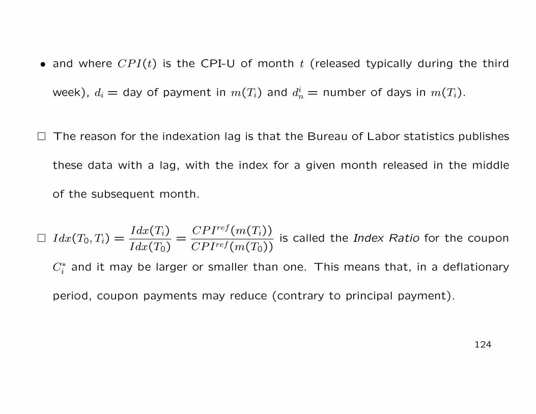
• and where CPI(t) is the CPI-U of month t (released typically during the third
week), di = day of payment in m(Ti) and din = number of days in m(Ti).
� The reason for the indexation lag is that the Bureau of Labor statistics publishes
these data with a lag, with the index for a given month released in the middle
of the subsequent month.
� Idx(T0, Ti) =Idx(Ti)
Idx(T0)=
CPIref(m(Ti))
CPIref(m(T0))is called the Index Ratio for the coupon
C∗i and it may be larger or smaller than one. This means that, in a deflationary
period, coupon payments may reduce (contrary to principal payment).
124
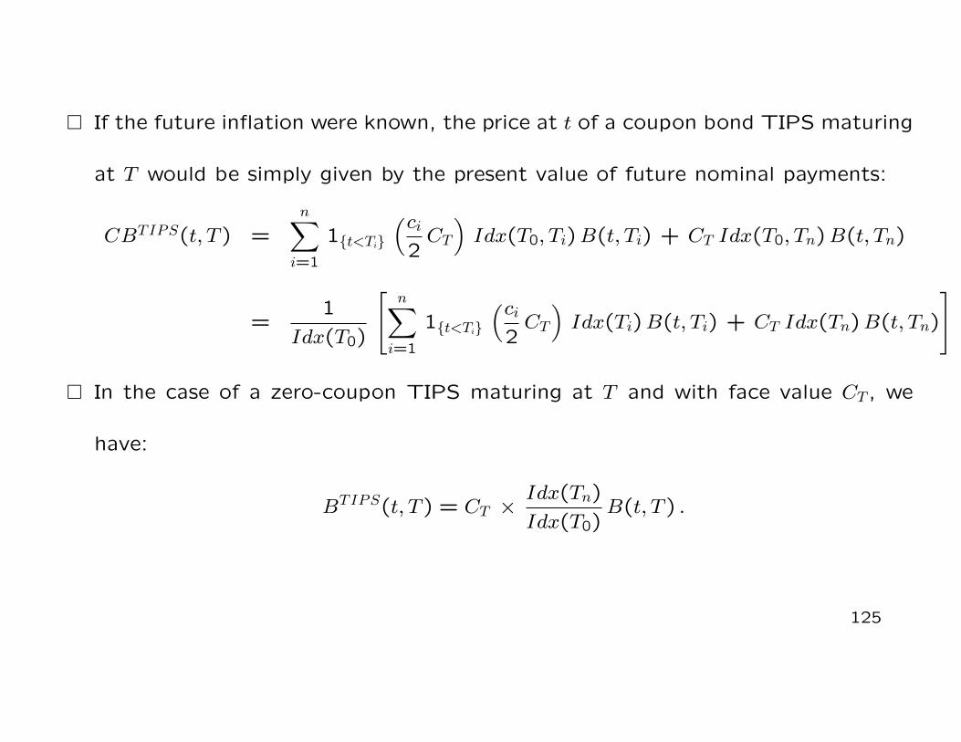
� If the future inflation were known, the price at t of a coupon bond TIPS maturing
at T would be simply given by the present value of future nominal payments:
CBTIPS(t, T ) =n∑i=1
1{t<Ti}
(ci2CT
)Idx(T0, Ti)B(t, Ti) + CT Idx(T0, Tn)B(t, Tn)
=1
Idx(T0)
[n∑i=1
1{t<Ti}
(ci2CT
)Idx(Ti)B(t, Ti) + CT Idx(Tn)B(t, Tn)
]
� In the case of a zero-coupon TIPS maturing at T and with face value CT , we
have:
BTIPS(t, T ) = CT ×Idx(Tn)
Idx(T0)B(t, T ) .
125
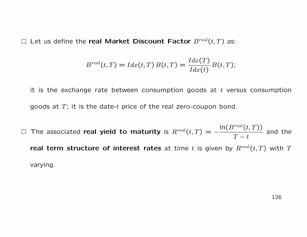
� Let us define the real Market Discount Factor Breal(t, T ) as:
Breal(t, T ) = Idx(t, T )B(t, T ) =Idx(T )
Idx(t)B(t, T );
it is the exchange rate between consumption goods at t versus consumption
goods at T ; it is the date-t price of the real zero-coupon bond.
� The associated real yield to maturity is Rreal(t, T ) = −ln(Breal(t, T ))
T − tand the
real term structure of interest rates at time t is given by Rreal(t, T ) with T
varying.
126
� The date-t value (in consumption goods) of the real coupon bond maturing at
T is given by:
CBreal(t, T ) =n∑i=1
1{t<Ti}
(ci2CT
)Breal(t, Ti) + CT B
real(t, Tn)
� From these results we can easily write :
CBTIPS(t, T ) =Idx(t)
Idx(T0)
[n∑i=1
1{t<Ti}
(ci2CT
)Breal(t, Ti) + CT B
real(t, Tn)
]
and, in particular, we have:
BTIPS(t, T ) =Idx(t)
Idx(T0)CT B
real(t, Tn) .
127

� From Breal(t, T ) = Idx(t, T )B(t, T ) we have:
Idx(t)
Idx(T )exp[−Rreal(t, T ) (T − t)] = exp[−R(t, T ) (T − t)] .
� Now, if we denote by π the constant continuously compounded annualized in-
flation rate between t and T , that is:
Idx(T ) = Idx(t) exp(π (T − t))
we immediately obtain R(t, T ) = Rreal(t, T ) + π (under perfect foresight!).
128

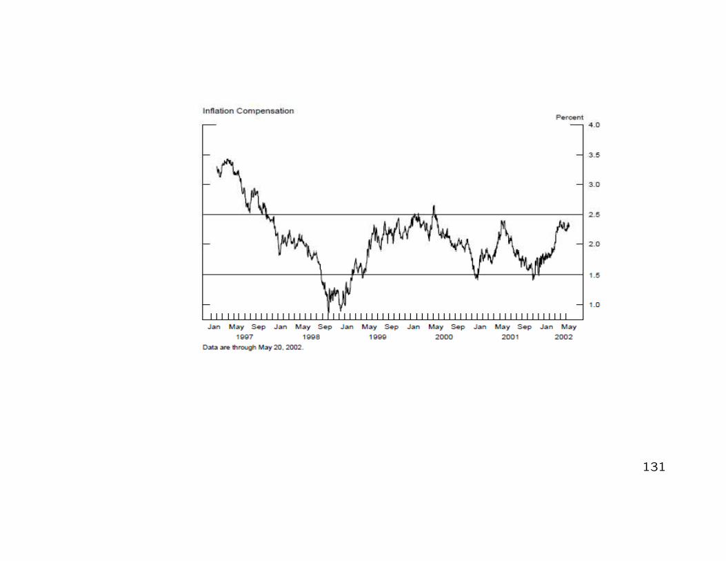
� In a general context where investors are risk-averse and there is uncertainty about
future inflation, the quantity
BEIR(t, T ) = R(t, T )−Rreal(t, T )
is called (spot) inflation compensation or Break Even Inflation Rate between
t and T .
� Remember that the BEIR IS NOT a measure of inflation expectations given
that it contains also inflation risk premium; BEIR is the sum of these two
components. The latter component refers to the risk that realized inflation may
deviate from the expected one.
129
130
131

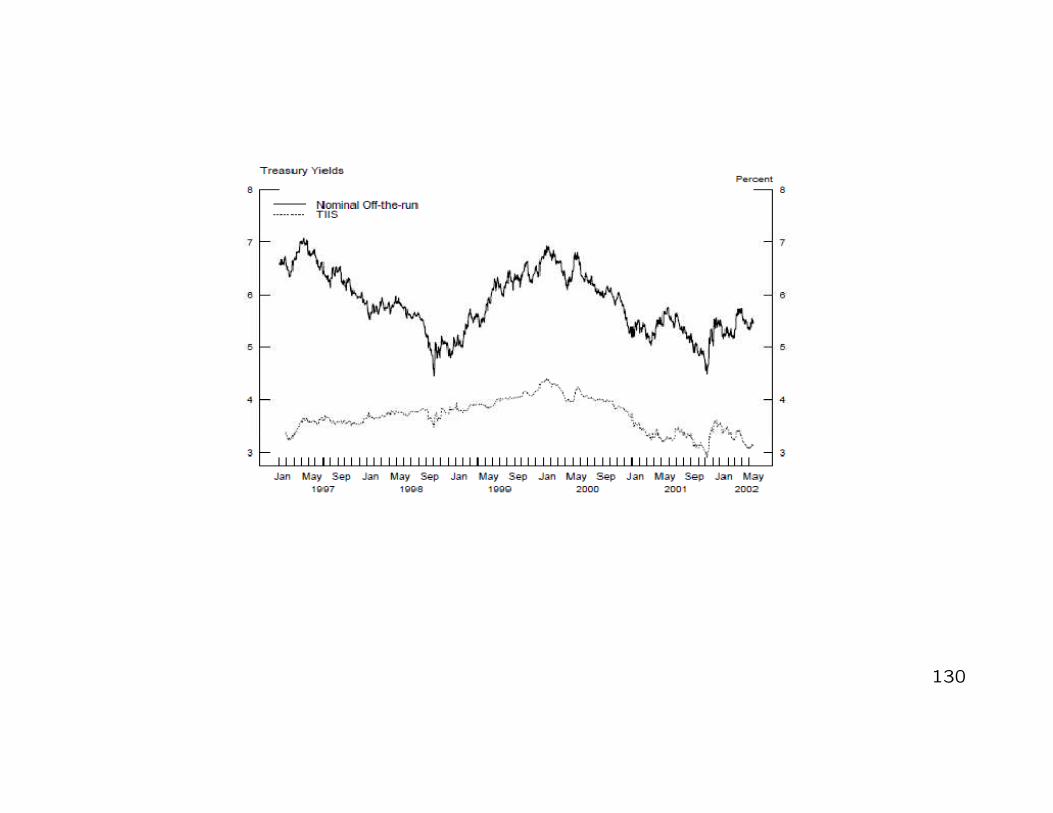
� These two last pictures are taken from Sack and Elsasser (2004): ”Treasury
Inflation-Indexed Debt: A Review of the U.S. Experience” available at
http://www.newyorkfed.org/research/epr/04v10n1/0405sack.pdf
� Nominal U.S. term structure of interest rates available at:
http://www.federalreserve.gov/pubs/feds/2006/200628/200628abs.html
� Real U.S. term structure of interest rates available at:
http://www.federalreserve.gov/pubs/feds/2008/200805/200805abs.html
132