five lectures on optimal transportation: geometry ... · five lectures on optimal transportation:...
TRANSCRIPT
FIVE LECTURES ON OPTIMAL TRANSPORTATION: GEOMETRY,REGULARITY AND APPLICATIONS
ROBERT J. MCCANN∗ AND NESTOR GUILLEN
Abstract. In this series of lectures we introduce the Monge-Kantorovich problem
of optimally transporting one distribution of mass onto another, where optimalityis measured against a cost function c(x, y). Connections to geometry, inequalities,
and partial differential equations will be discussed, focusing in particular on recent
developments in the regularity theory for Monge-Ampere type equations. An ap-plication to microeconomics will also be described, which amounts to finding the
equilibrium price distribution for a monopolist marketing a multidimensional line
of products to a population of anonymous agents whose preferences are known onlystatistically. c©2010 by Robert J. McCann. All rights reserved.
Contents
Preamble 21. An introduction to optimal transportation 21.1. Monge-Kantorovich problem: transporting ore from mines to factories 21.2. Wasserstein distance and geometric applications 31.3. Brenier’s theorem and convex gradients 41.4. Fully-nonlinear degenerate-elliptic Monge-Ampere type PDE 41.5. Applications 51.6. Euclidean isoperimetric inequality 51.7. Kantorovich’s reformulation of Monge’s problem 62. Existence, uniqueness, and characterization of optimal maps 62.1. Linear programming duality 82.2. Game theory 82.3. Relevance to optimal transport: Kantorovich-Koopmans duality 92.4. Characterizing optimality by duality 92.5. Existence of optimal maps and uniqueness of optimal measures 103. Methods for obtaining regularity of optimal mappings 113.1. Rectifiability: differentiability almost everywhere 123.2. From regularity a.e. to regularity everywhere 133.3. Regularity methods for the Monge-Ampere equation; renormalization 133.4. The continuity method (schematic) 144. Regularity and counterexamples for general costs 154.1. Examples 154.2. Counterexamples to the continuity of optimal maps 164.3. Monge-Ampere type equations 174.4. Ma-Trudinger-Wang conditions for regularity 184.5. Regularity results 194.6. Ruling out discontinuities: Loeper’s maximum principle 194.7. Interior Holder continuity for optimal maps 22
∗ [RJM]’s research was supported in part by grant 217006-08 of the Natural Sciences and EngineeringResearch Council of Canada.
1

2 ROBERT J. MCCANN∗ AND NESTOR GUILLEN
5. Multidimensional screening: an application to economic theory 235.1. Monopolist nonlinear pricing and the principal-agent framework 235.2. Variational formulation using optimal transportation 245.3. When is this optimization problem convex? 255.4. Variant: maximizing social welfare 266. A pseudo-Riemannian and symplectic geometric afterword 27References 28
Preamble
This survey is based on a series of five lectures by Robert McCann (of the Universityof Toronto), delivered at a summer school on “New Vistas in Image Processing andPartial Differential Equations” organized 7-12 June 2010 by Irene Fonseca, GiovanniLeoni, and Dejan Slepcev of Carnegie Mellon University on behalf of the Center forNonlinear Analysis there. The starting point for the manuscript which emerged was adetailed set of notes taken during those lectures by Nestor Guillen (University of Texasat Austin).
These notes are intended to convey a flavor for the subject, without getting boggeddown in too many technical details. Part of the discussion is therefore impression-istic, and some of the results are stated under the tacit requirement that the sup-ports of the measures µ± be compact, with the understanding that they extend tonon-compactly supported measures under appropriate hypotheses [93] [59] [45] [46]concerning the behaviour near infinity of the measures and the costs. The choice oftopics to be covered in a series of lectures is necessarily idiosyncratic. General ref-erences for these and other topics include papers of the first author posted on thewebsite www.math.toronto.edu/mccann and the two books by Villani [138] [139]. Ear-lier surveys include the ones by Ambrosio [4], Evans [43], Urbas [136] and Rachev andRuschendorf [115]. Many detailed references to the literature may be found there, toaugment the bibliography of selected works included below.
1. An introduction to optimal transportation
1.1. Monge-Kantorovich problem: transporting ore from mines to factories.The problem to be discussed can be caricatured as follows: imagine we have a distrib-ution of iron mines across the countryside, producing a total of 1000 tonnes of iron oreweekly, and a distribution of factories across the countryside that consume a total of1000 tonnes of iron ore weekly. Knowing the cost c(x, y) per ton of ore transported froma mine at x to a factory at y, the problem is to decide which mines should be supplyingwhich factories so as to minimize the total transportation costs.
To model this problem mathematically, let the triples (M±, d±, ω±) denote two com-plete separable metric spaces M± — also called Polish spaces — equipped with distancefunctions d± and Borel reference measures ω±. These two metric spaces will representthe landscapes containing the mines and the factories. They will often be assumedto be geodesic spaces, and/or to coincide. Here a geodesic space M(= M±) refersto a metric space in which every pair of points x0, x1 ∈ M is connected by a curves ∈ [0, 1] → xs ∈ M satisfying
(1) d(x0, xs) = sd(x0, x1) and d(xs, x1) = (1− s)d(x0, x1) ∀ s ∈ [0, 1].
Such a curve is called a geodesic segment.
OPTIMAL TRANSPORTATION: GEOMETRY, REGULARITY AND APPLICATIONS 3
e.g. 1) Euclidean space: M = Rn, d(x, y) = |x − y|, ω = V ol = Hn = Hausdorffn-dimensional measure, geodesic segments take the form xs = (1− s)x0 + sx1.
e.g. 2) Complete Riemannian manifold (M = M±, gij), with or without boundary:dω = dV ol = dHn = (det gij)1/2dnx,
12d2(x0, x1) = inf
{xs|x(0)=x0,x(1)=x1}
12
∫ 1
0
〈xs, xs〉g(xs)ds.
A minimizing curve s ∈ [0, 1] 7−→ xs ∈ M exists by the Hopf-Rinow theorem; it satisfies(1), and is called a Riemannian geodesic.
The distributions of mines and factories will be modeled by Borel probability mea-sures µ+ on M+ and µ− on M−, respectively. Any Borel map G : M+ −→ M− definesan image or pushed-forward measure ν = G#µ+ on M− by
(2) (G#µ+)[V ] := µ+[G−1(V )] ∀ V ⊂ M−.
A central problem in optimal transportation is to find, among all maps G : M+ −→ M−
pushing µ+ forward to µ−, one which minimizes the total cost
(3) cost (G) =∫
M+c(x,G(x))dµ+(x).
This problem was first proposed by Monge in 1781, taking the Euclidean distancec(x, y) = |x − y| as his cost function [104]. For more generic costs, some basic math-ematical issues such as the existence, uniqueness, and mathematical structure of theoptimizers are addressed in the second lecture below. However nonlinearity of the ob-jective functional and a lack of compactness or convexity for its domain make Monge’sformulation of the problem difficult to work with. One and a half centuries later, Kan-torovich’s relaxation of the problem to an (infinite-dimesional) linear program provideda revolutionary tool [67] [68].
1.2. Wasserstein distance and geometric applications. The minimal cost of trans-port between µ+ and µ− associated to c(·, ·) will be provisionally denoted by
(4) Wc(µ+, µ−) = infG#µ+=µ−
cost (G).
It can be thought of as quantifying the discrepancy between µ+ and µ−, and is moreproperly defined using Kantorovich’s formulation (11), though we shall eventually showthe two definitions coincide in many cases of interest. When M = M±, the costsc(x, y) = dp(x, y) with 0 < p < 1 occur naturally in economics and operations research,where it is often the case that there is an economy of scale for long trips [96]. In thiscase, the quantity Wc(µ+, µ−) defines a metric on the space P(M) of Borel probabilitymeasures on M . For p ≥ 1 on the other hand, it is necessary to extract a p-th root toobtain a metric
(5) dp(µ+, µ−) := Wc(µ+, u−)1/p
on P(M) which satisfies the triangle inequality.Though the initial references dealt specifically with the case p = 1 [69] [142], the whole
family of distances are now called Kantorovich-Rubinstein or Wasserstein metrics [41].Apart from the interesting exception of the limiting case d∞ = limp→∞ dp [98] [26], on acompact metric space M all these metrics give rise to the same topology, namely weak-∗convergence. For non-compact M , the dp topologies differ from each other only in thenumber of moments of a sequence of measures which are required to converge. Moreover,(P(M), dp) inherits geometric properties from (M,d), such as being a geodesic space.Notions such as Ricci curvature in the underlying space (M,d) can be characterized by

4 ROBERT J. MCCANN∗ AND NESTOR GUILLEN
the geodesic convexity first explored in [94] of certain functionals on the larger spaceP(M) — such as Boltzmann’s entropy. One direction of this equivalence was provedby Cordero-Erausquin, McCann, and Schmuckenschager [30] and Otto and Villani [110]in projects which were initially independent (see also [28] and [31]), while the conversewas established by von Renesse and Sturm [116] confirming the formal arguments of[110]. This equivalence forms the basis of Lott-Villani and Sturm’s definition of lowerbounds for Ricci curvature in the metric measure space setting, without reference to anyunderlying Riemannian structure [88] [127]. McCann and Topping used a similar idea tocharacterize the Ricci flow [99], which led Lott [87] and Topping [130] to simpler proofsof Perelman’s celebrated monotonicity results [112]. Despite the interest of these recentdevelopments, we shall not pursue them farther in these lectures, apart from sketchinga transportation-based proof of the isoperimetric theorem whose ideas underpin manysuch geometric connections.
1.3. Brenier’s theorem and convex gradients. It turns out that Monge’s costc(x, y) = |x − y| is among the hardest to deal with, due to its lack of strict con-vexity. For this cost, the minimizer of (4) is not generally unique, even on the lineM± = R. Existence of solutions is tricky to establish: the first ‘proof’, due to Sudakov[128], relied on an unsubstantiated claim which turned out to be correct only in theplane M± = R2 [11]; higher dimensional arguments were given increasing generalityby Evans-Gangbo [44], and then Ambrosio [4], Caffarelli-Feldman-McCann [21], andTrudinger-Wang [132] independently. Simpler approaches were proposed by Champion-DePascale [25] and Bianchini-Cavalletti [11] more recently.
The situation for the quadratic cost c(x, y) = |x− y|2 is much simpler, mirroring therelative simplicity of the Hilbert geometry of L2 among Banach spaces Lp with p ≥ 1.Brenier [14] [15] (and others around the same time [114] [124] [33] [123] [34] [1]) showedthat there is a unique [34] [1] solution [33] , and characterized it as a convex gradient[114] [124] [123].
Theorem 1.1 (A version of Brenier’s theorem). If µ+ � dV ol and µ− are Borelprobability measures on M± = Rn, then there exists a convex function u : Rn →R ∪ {+∞} whose gradient G = Du : Rn → Rn pushes µ+ forward to µ−. Apart fromchanges on a set of measure zero, G is the only map to arise in this way. Moreover, Guniquely minimizes Monge’s problem (4) for the cost c(x, y) = |x− y|2.
Remark: In this generality the theorem was established by McCann [93], where theassumption µ+ � dV ol was also relaxed. A further relaxation by Gangbo-McCann [59]is shown to be sharp in Gigli [61].
1.4. Fully-nonlinear degenerate-elliptic Monge-Ampere type PDE. How dopartial differential equations (more specifically, fully nonlinear degenerate elliptic PDE)enter the picture? Let’s consider the constraint G#µ+ = µ−, assuming moreover thatµ± = f±dV ol± on Rn or on Riemannian manifolds M±. Then if φ ∈ C(M−) is a testfunction, it follows that∫
M+φ(G(x))f+(x)dV ol+(x) =
∫M−
φ(y)f−(y)dV ol−(y).
If G was a diffeomorphism, we could combine the Jacobian factor dny = |detDG(x)|dnxfrom the change of variables y = G(x) with arbitrariness of φ ◦G to conclude f+(x) =|det DG(x)|f−(G(x)) for all x. We will actually see that this nonlinear equation holdsf+-a.e. as a consequence of Theorem 3.2.

OPTIMAL TRANSPORTATION: GEOMETRY, REGULARITY AND APPLICATIONS 5
In the case of Brenier’s map G(x) = Du(x), convexity of u implies non-negativity ofthe Jacobian DG(x) = D2u(x) ≥ 0. It also guarantees almost everywhere differentia-bility of G by Alexandrov’s theorem (or by Lebesgue’s theorem in one dimension); seeTheorem 3.2 for the sketch of a proof. Thus u solves the Monge-Ampere equation [15]
(6) f+(x) = det(D2u(x))f−(Du(x))
a.e. [94] subject to the condition Du(x) ∈ M− for x ∈ M+. This is known as the 2ndboundary value problem in the partial differential equations literature. We shall see thatlinearization of this equation around a convex solution leads to a (degenerate) ellipticoperator (29), whose ellipticity becomes uniform if the solution u is smooth and stronglyconvex, meaning positivity of its Hessian is strict: D2u(x) > 0.
1.5. Applications. The Monge-Kantorovich theory has found a wide variety of appli-cations in pure and applied mathematics. On the pure side, these include connectionsto inequalities [92] [131] [94] [32] [90] [52], geometry (including sectional [85] [73], Ricci[88] [87] [127] [99] and mean [75] curvature), nonlinear partial differential equations [14][18] [16] [135] [89], and dynamical systems (weak KAM theory [9]; nonlinear diffusions[109]; gradient flows [5]). On the applied side these include applications to vision (im-age registration and morphing [64]), economics (equilibration of supply with demand[42] [27], structure of cities [23], maximization of profits [118] [22] [49] or social welfare[49]), physics [40] [129] [95] [51], engineering (optimal shape / material design [12] [13],reflector antenna design [63] [140] [141], aerodynamic resistance [113]), atmosphere andocean dynamics (the semigeostrophic theory [36] [37] [35]), biology (irrigation [10], leafgrowth [143]), and statistics [115]. See [138] [139] for further directions, references, anddiscussion.
1.6. Euclidean isoperimetric inequality. It was observed (independently by Mc-Cann [92] [94] and Trudinger [131]) that a solution to the second boundary value problemfor the Monge-Ampere equation (6) yields a simple proof of the isoperimetric inequality(with its sharp constant): for M+ ⊂ Rn
(7) V ol(M+) = V ol(B1) ⇒ Hn−1(∂M+) ≥ Hn−1(∂B1).
The following streamlined argument was perfected later; it combines optimal maps withan earlier approach from Gromov’s appendix to [101].
Proof. Take f+ = χM+ and f− = χB1 to be uniformly distributed. Brenier’s theoremthen gives a volume-preserving map G = Du between M+ and B1:
1 = det1/n(D2u(x)).
The expression on the right is the geometric mean of the eigenvalues of D2u(x), whichare non-negative by convexity of u, so the arithmetic-geometric mean inequality yields
(8) 1 ≤ (arithmetic mean of eigenvalues) =1n
∆u
almost everywhere in M+. (The right hand side is the absolutely continuous part of thedistributional Laplacian; convexity of u allows it to be replaced by the full distributionalLaplacian of u without spoiling the inequality.) Integrating inequality (8) on M+ yields
(9) V ol(M+) ≤ 1n
∫M+
∆u dnx =1n
∫∂M+
Du(x) · nM+(x)dHn−1(x).

6 ROBERT J. MCCANN∗ AND NESTOR GUILLEN
Now, since G = Du ∈ B1 whenever x ∈ M+, we have |Du| ≤ 1, thus V ol(M+) =V ol(B1) gives
(10) V ol(B1) ≤1n
∫∂M+
1 dHn−1 =1nHn−1(∂M+).
In the case special M+ = B1, Brenier’s map coincides with the identity map so equalitieshold throughout (8)–(10), yielding the desired conclusion (7)! �
As the preceding proof shows, one of the important uses of optimal transportation inanalysis and geometry is to encode non-local ‘shape’ information into a map which canbe localized, reducing global geometric inequalities to algebraic inequalities under anintegral. For subsequent developments in this direction, see works of Ambrosio, Cordero-Erausquin, Carrillo, Figalli, Gigli, Lott, Maggi, McCann, Nazaret, Otto, Pratelli, vonRenesse, Schmuckenschlager, Sturm, Topping and Villani in [95] [110] [30] [31] [32] [5][24] [116] [127] [88] [87] [99] [52].
1.7. Kantorovich’s reformulation of Monge’s problem. Now let us turn to theproof of Brenier’s theorem and the ideas it involves. A significant breakthrough wasmade by Kantorovich [67] [68], who relaxed our optimization problem (the Monge prob-lem), by dropping the requirement that all the ore from a given mine goes to a singlefactory. In other words:
Replace G : M+ → M− by a measure 0 ≤ γ on M+ ×M− whose marginals are µ+
and µ−, respectively, and among such measures choose γ to minimize the functional
cost (γ) =∫
M+×M−c(x, y)dγ(x, y).
Such a joint measure γ is also known as a “transport plan” (in analogy with“transportmap”). This is better than Monge’s original formulation for at least two reasons:
1) The functional to be minimized now depends linearly on γ.
2) The set Γ(µ+, µ−) of admissible competitors γ is a convex subset of a suitableBanach space: namely, the dual space to continuous functions (C(M+ ×M−), ‖ · ‖∞)(which decay to zero at infinity in case the compactness of M± is merely local).
In this context, well-known results in functional analysis guarantee existence of aminimizer γ under rather general hypotheses on c and µ±. Our primary task will beto understand when the solution will be unique, and to characterize it. At least oneminimizer will be an extreme point of the convex set Γ(µ+, µ−), but its uniquenessremains an issue. Necessary and sufficient conditions will come from the duality theoryof (infinite dimensional) linear programming [6] [70].
2. Existence, uniqueness, and characterization of optimal maps
Let’s get back to the Kantorovich problem:
(11) Wc(µ+, µ−) := minγ∈Γ(µ+,µ−)
∫M+×M−
c(x, y)dγ(x, y) = minγ∈Γ(µ+,µ−)
cost (γ)
The basic geometric object of interest to us will be the support spt γ := S of a com-petitor γ, namely the smallest closed subset S ⊂ M+×M− carrying the full mass of γ.

OPTIMAL TRANSPORTATION: GEOMETRY, REGULARITY AND APPLICATIONS 7
What are some of the competing candidates for the minimizer?
eg.1) Product measure: µ+ ⊗ µ− ∈ Γ(µ+, µ−), for which spt γ = spt µ+ × spt µ−.
eg.2) Monge measure: if G : M+ → M− with G#µ+ = µ− then id × G : M+ −→M+ ×M− and γ = (id×G)#µ+ ∈ Γ(µ+, µ−) has cost (γ) = cost (G).
The second example shows in what sense Kantorovich’s formulation is a relaxation ofMonge’s problem, and why (4) must be at least as big as (11). In this example spt γ willbe the (closure of the) graph of G : M+ −→ M−, which suggests how Monge’s map Gmight in principle be reconstructed from a minimizing Kantorovich measure γ. Beforeattempting this, let us recall a notion which characterizes optimality in the Kantorovichproblem.
Definition 2.1 (c-cyclically monotone sets). S ⊂ M+ ×M− is c-cyclically monotoneif and only if all k ∈ N and (x1, y1), ..., (xk, yk) ∈ S satisfy
(12)k∑
i=1
c(xi, yi) ≤k∑
i=1
c(xi, yσ(i))
for each permutation σ of k letters.
The following result was deduced by Smith and Knott [125] from a theorem ofRuschendorf [120]. A more direct proof was given by Gangbo and McCann [59]; itsconverse is true as well.
Theorem 2.2 (Smith and Knott ’92). If c ∈ C(M+ × M−), then optimality of γ ∈Γ(µ+, µ−) implies spt γ is a c-cyclically monotone set.
The idea of the proof in [59] is that if spt γ is not cyclically monotone, then settingoi = (xi, yi) and zi = (xi, yσ(i)) we could with some care define a perturbation
γε = γ + ε(near the z’s)− ε(near the o’s)
in Γ(µ+, µ−) of γ for which cost (γε) < cost (γ0), thus precluding the optimality of γ.
e.g. If c(x, y) = −x · y or c(x, y) = 12 |x− y|2 then (12) becomes
k∑i=1
〈yi, xi − xi−1〉 ≥ 0
with the convention x0 := xk. This is simply called cyclical monotonicity, and can beviewed as a discretization of ∮
y(x) · dx ≥ 0,
a necessary and sufficient condition for the vector field y(x) to be conservative, meaningy = Du(x). This heuristic underlies a theorem of Rockafellar [119]:
Theorem 2.3 (Rockafellar ’66). The set S ⊂ Rn ×Rn is cyclically monotone if andonly if there exists a convex function u : Rn → R ∪ {∞} such that S ⊂ ∂u where
(13) ∂u := {(x, y) ∈ Rn ×Rn | u(z) ≥ u(x) + 〈z − x, y〉+ o(|z − x|) ∀z ∈ Rn}.The subdifferential ∂u defined by (13) consists of the set of (point, slope) pairs for
which y is the slope of a hyperplane supporting the graph of u at (x, u(x)).
Remark 2.4 (Special case (monotonicity)). Note that when c(x, y) = −x · y and k = 2,(12) implies for all (x1, y1), (x2, y2) ∈ S that
(14) 〈∆x,∆y〉 := 〈x2 − x1, y2 − y1〉 ≥ 0.
This condition implies that y2 is constrained to lie in a halfspace with y1 on its boundaryand ∆x as its inward normal. Should y = Du(x) already be known to be conservative,the monotonicity inequalities (14) alone become equivalent to convexity of u.

8 ROBERT J. MCCANN∗ AND NESTOR GUILLEN
2.1. Linear programming duality. An even more useful perspective on these linearprogramming problems is given by the the duality theorem discovered by Kantorovich[67] and Koopmans [76] — for which they later shared the Nobel Memorial Prize ineconomics. It states that our minimization problem is equivalent to a maximizationproblem
(15) minγ∈Γ(µ+,µ−)
∫M+×M−
c dγ = sup(−u,−v)∈Lipc
−∫
M+u(x) dµ+(x)−
∫M−
v(y) dµ−(y).
Here
Lipc = {(u+, u−) with u± ∈ L1(M±, dµ±) | c(x, y) ≥ u+(x)+u−(y) ∀(x, y) ∈ M+×M−}.One of the two inequalities (≥) in (15) follows at once from the definition of −(u, v) ∈
Lipc by integratingc(x, y) ≥ −u(x)− v(y)
against γ ∈ Γ(µ+, µ−). The magic of duality is that equality holds in (15).
2.2. Game theory. Some intuition for why this magic works can be gleaned from thethe theory of (two-player, zero-sum) games. In that context, Player 1 chooses strategyx ∈ X, Player 2 chooses strategy y ∈ Y , and the outcome is that Player 1 pays P (x, y)to Player 2. The payoff function P ∈ C(X×Y ) is predetermined and known in advanceto both players; P1 wants to minimize the resulting payment and P2 wants to maximizeit.
Now, what if one the players declares his or her strategy (x or y) to the other playerin advance? If P1 declares first, the outcome is better for P2, who has a chance tooptimize his response to the announced strategy x, and conversely. This implies that
(16) infx∈X
supy∈Y
P (x, y) ≥ supy∈Y
infx∈X
P (x, y);
(Player 1 declares first vs player 2 declares first.) Von Neumann [107] identified struc-tural conditions on the payoff function to have a saddle point (17), in which case equalityholds in (15); see also Kakutani’s reference to [108] in [66].
Theorem 2.5 (convex/concave min-max). If X ⊂ Rm and Y ⊂ Rn are compact andconvex, then equality holds in (16) provided for each (x0, y0) ∈ X × Y both functionsx ∈ X 7−→ P (x, y0) and y ∈ Y 7−→ −P (x0, y) are convex. (In fact, convexity of allsublevel sets of both functions is enough.)
Proof. Letxb(y) ∈ arg min
x∈XP (x, y) yb(x) ∈ arg max
y∈YP (x, y)
denote the best responses of P1 and P2 to each other’s strategies y and x. Note xb andyb are continuous if the convexity and concavity assumed of the payoff function are bothstrict. In that case, Brouwer’s theorem asserts the the function yb ◦ xb : Y → Y has afixed point y0. Setting x0 = xb(y0), since y0 = yb(x0) we have found a saddle point
(17) infx∈X
maxy∈Y
P (x, y) ≤ maxy∈Y
P (x0, y) = P (x0, y0) = minx∈X
P (x, y0) ≤ supy∈Y
minx∈X
P (x, y)
of the payoff function, which proves equality holds in (16). If the convexity and concavityof the payoff function are not strict, apply the theorem just proved to the perturbedpayoff Pε(x, y) = P (x, y) + ε(|x|2 − |y|2) and take the limit ε → 0. �
e.g. Expected payoff [107]: von Neumann’s original example of a function to which thetheorem and its conclusion applies is the expected payoff P (x, y) =
∑mi=1
∑nj=1 pijxiyj
of mixed or randomized strategies x and y for a game in which P1 and P2 each haveonly finitely many pure strategies, and the payoff corresponding to strategy 1 ≤ i ≤ m
OPTIMAL TRANSPORTATION: GEOMETRY, REGULARITY AND APPLICATIONS 9
and 1 ≤ j ≤ n is pij . In this case X = {x ∈ [0, 1]m |∑
xi = 1} and Y = {y ∈[0, 1]n |
∑yj = 1} are standard simplices of the appropriate dimension, whose vertices
correspond to the pure strategies.
2.3. Relevance to optimal transport: Kantorovich-Koopmans duality. Infinitedimensional versions of von-Neumann’s theorem can also be formulated where X andY lie in Banach spaces; they are proved using Schauder’s fixed point theorem instead ofBrouwer’s. A payoff function germane to optimal transportation is defined on the strat-egy spaces X = {0 ≤ γ on M+ ×M−} and Y = {(u, v) ∈ L1(M+, µ+)⊕ L1(M−, µ−)}by
P (γ, (u, v)) =∫
M+×M−(c(x, y) + u(x) + v(y)) dγ(x, y)−
∫M+
udµ+ −∫
M−vdµ−.
Note the bilinearity of P on X × Y . Since
infγ∈X
P (γ, (u, v)) ={−∞ unless (−u,−v) ∈ Lipc,0−
∫udµ+ −
∫vdµ− otherwise,
the Kantorovich-Koopmans dual problem is recovered from the version of the game inwhich P2 is compelled to declare his strategy first:
(18) sup(u,v)∈Y
infγ∈X
P (γ, (u, v)) = sup(−u,−v)∈Lipc
∫(−u)dµ+ +
∫(−v)dµ−.
On the other hand, rewriting
P (γ, (u, v)) =∫
M+×M−cdγ +
∫u(dγ − dµ+) +
∫v(y)(dγ(x, y)− dµ−(y))
we see
(19) sup(u,v)∈Y
P (γ, (u, v)) ={
+∞ unless γ ∈ Γ(µ+, µ−)∫M+×M− c dγ if γ ∈ Γ(µ+, µ−).
Thus the primal transportation problem of Kantorovich and Koopmans
infγ∈X
sup(u,v)∈Y
P (γ, (u, v)) = infγ∈Γ(µ+,µ−)
∫M+×M−
c dγ
corresponds to the version of the game in which P1 declares his strategy first. The equal-ity between (18) and (19) asserted by an appropriate generalization of von Neumann’stheorem implies the duality (15):
minγ∈Γ(µ+,µ−)
∫M+×M−
cdγ = sup(−u,−v)∈Lipc
∫M+
(−u)dµ+ +∫
M−(−v)dµ−.
2.4. Characterizing optimality by duality. The following theorem can be deducedas an immediate corollary of this duality. We may think of the potentials u and vas being Lagrange multipliers enforcing the constraints on the marginals of γ; in theeconomics literature they are interpreted as shadow prices which reflect the geographicvariation in scarcity or abundance of supply and demand. The geography is encoded inthe choice of cost.
Theorem 2.6 (Necessary and sufficient conditions for optimality). The existence of−(u, v) ∈ Lipc such that γ vanishes outside the zero set of the non-negative functionk(x, y) = c(x, y) + u(x) + v(y) ≥ 0 on M+ × M− is necessary and sufficient for theoptimality of γ ∈ Γ(µ+, ν−) with respect to c ∈ C(M+ ×M−).

10 ROBERT J. MCCANN∗ AND NESTOR GUILLEN
Corollary 2.7 (First and second order conditions on potentials). Optimality of γ and(u, v) implies Dk = 0 and D2k ≥ 0 at any point (x, y) ∈ spt γ where these derivativesexist. In particular, Dx[c(x, y) + u(x) + v(y)] = 0 and D2
x[c(x, y) + u(x) + v(y)] ≥ 0holds γ-a.e., and likewise for y-derivatives.
e.g. Consider the special case of the bilinear cost: c(x, y) = −x · y. Here the first andsecond order conditions of the corollary become
y = Du(x) and D2u(x) ≥ 0,
suggesting y is the graph of the gradient of a convex function. In this case, convexityof u guarantees D2u is defined a.e. with respect to Lebesgue measure, by Alexandrov’stheorem.
2.5. Existence of optimal maps and uniqueness of optimal measures. Moregenerally, we claim u inherits Lipschitz and semiconvexity bounds (23)–(24) from c(x, y),which guarantee the existence of x-derivatives in the preceding corollary — at leastLebesgue almost everywhere. This motivates the following theorem of Gangbo [57] andLevin [80]; variations appeared independently in Caffarelli [16], Gangbo and McCann[58] [59], and Ruschendorf [121] [122] at around the same time, and subsequently in [89].
Definition 2.8 (Twist conditions). A function c ∈ C(M+ × M−) differentiable withrespect to x ∈ M+ is said to be twisted if
(20) (A1)+ ∀ x0 ∈ M+, the map y ∈ M− 7−→ Dxc(x0, y) ∈ T ∗x M+ is one-to-one.
For (x, p) ∈ T ∗M+ denote the unique y ∈ M− solving Dxc(x, y) + p = 0 by y = Y (x, p)when it exists. When the same condition holds for the cost c(y, x) := c(x, y), we denoteit by (A1)−. When both c and c satisfy (A1)+, we say the cost is bi-twisted, and denotethis by (A1).
Theorem 2.9 (Existence of Monge solutions; uniqueness of Kantorovich solutions).Fix Polish probability spaces (M±, µ±) and assume M+ is a n-dimensional manifoldand dµ+ � dnx is absolutely continuous (in coordinates). Let c ∈ C(M+×M−) differ-entiable with respect to x ∈ M+ satisfy the twist condition (20) and assume Dxc(x, y) isbounded locally in x ∈ M+ uniformly in y ∈ M−. Then, there exists a locally Lipschitz(moreover, c-convex, as in Definition 2.10) function u : M+ → R such that
a) G(x) := Y (x,Du(x)) pushes µ+ forward to µ−;
b) this map is unique, and uniquely solves Monge’s minimization problem (4);
c) Kantorovich’s minimization (11) has a unique solution γ;
d) γ = (id×G)#µ+.
Definition 2.10 (c-convex). A function u : M+ −→ R∪{+∞} (not identically infinite)is c-convex if and only if u = (uc)c, where
(21) uc(y) = supx∈M+
−c(x, y)− u(x) and vc(x) = supy∈M−
−c(x, y)− v(y).
Remark 2.11 (Legendre-Fenchel transform and convex dual functions). When c(x, y) =−〈x, y〉, then uc(y) is manifestly convex: it is the Legendre-Fenchel transform or convexdual function of u(x). In this case, (uc)c is well-known to yield the lower semicontinuousconvex hull of the graph of u, so that u = (uc)c holds if and only if u is already lowersemicontinuous and convex. More generally, we interpret the condition u = ucc as beingthe correct adaptation of the notion of convexity to the geometry of the cost function c.

OPTIMAL TRANSPORTATION: GEOMETRY, REGULARITY AND APPLICATIONS 11
Sketch of proof of Theorem 2.9. The key idea of the proof is to establish existence of amaximizer −(u, v) ∈ Lipc of (15) with the additional property that (u, v) = (vc, uc).Differentiability of u = ucc on a set dom Du of full dµ+ � dnx measure then follows fromRademacher’s theorem and Lemma 3.1. The map G(x) := Y (x,Du(x)) is well-definedon dom Du by the twist condition (assuming the supremum (21) defining (uc)c(x) isattained). Corollary 2.7 shows any minimizer γ vanishes outside the graph of this map,and it then follows easily that γ = (id×G)#µ+ and hence γ is uniquely determined by u
[2]. Conversely any other c-convex u for which G(x) = Y (x, Du(x)) pushes µ+ forwardto µ− can be shown to maximize the dual problem by checking that γ = (id× G)#µ+
vanishes outside the support of G. Thus γ = γ and G = G holds µ+-a.e.To extract the desired −(u, v) ∈ Lipc from a maximizing sequence −(uk, vk) requires
some compactness. (This would come from the convexity of uk and vk in case c(x, y) =−x · y via the Blaschke selection theorem.) Observe −(u, v) ∈ Lipc implies
u(x) ≥ supy∈M−
−c(x, y)− v(y) =: vc(x).
Moreover, −(vc, v) ∈ Lipc and −(vc) ≥ −u can only increase the value of the objectivefunctional relative to −(u, v). Thus −(vc, v) is a better candidate for a maximizer than−(u, v). Repeating the process shows −(vc, vcc) and −(vccc, vcc) ∈ Lipc are betterstill, since (vc)c ≤ v and (vcc)c ≤ vc by the same logic. On the other hand, startingfrom vcc ≤ v, the negative coefficient in definition (21) implies the opposite inequality(vcc)c ≥ vc. Thus vccc = vc quite generally. (This is precisely analogous to the fact thatthe second Legendre transform u∗∗ does not change a function u = v∗ which is alreadyconvex and lower semicontinuous; see Remark 2.11.)
Replacing a maximizing sequence −(uk, vk) with −(vck, vcc
k ) therefore yields a newmaximizing sequence at least as good which moreover consists of c-convex functions.Lemma 3.1 shows this new family is locally equi-Lipschitz, hence we only need localboundedness for the Arzela-Ascoli theorem to yield a limiting maximizer −(u, v), whichwill in fact be c-convex, though we can also replace it by −(vc, vcc) just to be sure.Local boundedness also follows from Lemma 3.1, after fixing x0 ∈ spt µ+ ⊂ M+ andreplacing −(uk, vk) by −(uk − λk, vk + λk) with λk = uk(x0). This replacement doesnot change the value of the objective functional (18), yet ensures that u(x0) = 0. �
3. Methods for obtaining regularity of optimal mappings
Given mines and factories (M±, µ±) and a cost function c ∈ C(M+ ×M−), in thepreceding section we found conditions which guarantee the existence and uniqueness ofa map G(x) = Y (x, Du(x)) such that G#µ+ = µ− with u = ucc, ie. c-convex. Under thesame conditions, the map G is the unique minimizer of Monge’s problem (4). The spaceM+ was assumed to be an n-dimensional manifold, and the following twist hypothesis(A1)+, equivalent to (20), was crucial to specifying Y (x, ·):
(22) ∀ y1 6= y2 ∈ M− assume x ∈ M+ 7−→ c(x, y1)− c(x, y2) has no critical points.
Notice, however, that (22) cannot be satisfied by any cost function which is differen-tiable throughout a compact manifold M+. In case M+ = Sn, Monge solutions do notgenerally exist [60], but criteria are given in [27] [2] which guarantee uniqueness of theKantorovich minimizer. On the other hand, it is an interesting open problem to find acriterion on c ∈ C1(M+ ×M−) which guarantees uniqueness of Kantorovich solutionsfor all µ± ∈ L1(M±) in more complicated topologies, such as the torus M± = Tn forexample. Here differentiability of the cost function is crucial; for costs such as Riemann-ian distance squared, the desired uniqueness is known [29] [97], but the cost fails to bedifferentiable at the cut locus.

12 ROBERT J. MCCANN∗ AND NESTOR GUILLEN
3.1. Rectifiability: differentiability almost everywhere. The current section isdevoted to reviewing methods for exploring the smoothness properties of the optimalmap G found above, or equivalently of its c-convex potential u. The following lemmashows that all c-convex functions inherit Lipschitz and semiconvexity properties directlyfrom the cost function c; it has already been exploited to prove Theorem 2.9.
Lemma 3.1 (Inherent regularity of c-convex functions). If u = ucc and c(·, y) ∈Ck
loc(M+) for each y ∈ M−, then k = 1 implies (23) and k = 2 implies (24):
|Du(x)| ≤ supy∈M−
|Dxc(x, y)| (local Lipschitz regularity);(23)
D2u(x) ≥ infy∈M−
−D2xxc(x, y) (semiconvexity).(24)
Similarly, c-cyclically monotone sets S ⊂ M+ × M− turn out to be containedin Lipschitz submanifolds of dimension n = dimM± when the cost function is non-degenerate (25). The following recent theorem of McCann-Pass-Warren [100] combineswith Rademacher’s theorem — which asserts the differentiability Lebesgue a.e. of Lip-schitz functions — to give a simple tool for establishing that f+(x) = |det(DG(x))|f−(G(x))holds f+-a.e.
Theorem 3.2 (Rectifiability of optimal transport [100]). Assume M± are n-dimensionalmanifolds, at least in a neighbourhood U of (x0, y0) ∈ M+×M−, where c ∈ C2(U) and
(25) (A2) detD2xiyj c(x0, y0) 6= 0.
If S ⊂ M+×M− is c-cyclically monotone, then S∩V lies in an n-dimensional Lipschitzsubmanifold, for some neighbourhood V ⊂ U of (x0, y0).
In view of Theorem 2.2, this conclusion applies either to the graph S = Graph(G)of any optimal map (4) or the support S = spt (γ) of any optimal measure (11) in thetransportation problem.
Figure 1: Optimizers have locally monotone support S in the plane.Motivation: on the line M± = R, without further assumptions on c or µ±, a transportmap may not exist nor be monotone, yet the theorem above says that even so all piecesof spt (γ) lie along along Lipschitz arcs in the plane. These curves will actually be locallymonotone — non-decreasing or non-increasing depending on the sign of D2
xyc(x0, y0);see Figure 1.
Idea of proof. Introduce the notation b = −c. In case c(x, y) = −x · y on M± = Rn,monotonicity asserts for all (x0, y0), (x1, y1) ∈ S that ∆x = x1 − x0 and ∆y = y1 − y0

OPTIMAL TRANSPORTATION: GEOMETRY, REGULARITY AND APPLICATIONS 13
satisfy
0 ≤ 〈∆x, ∆y〉 =⟨
∆z −∆w√2
,∆z + ∆w√
2
⟩where
(26) (z, w) := (x + y√
2,x− y√
2).
This implies that |∆w|2 ≤ |∆z|2 meaning w = w(z) has Lipschitz constant 1 as a graphover z ∈ Rn. Equivalently, S has Lipschitz constant 1 as a graph over the diagonal inM+ × M−. This special case was established by Alberti and Ambrosio [3], using anargument of Minty [102].
For more general costs b = −c and any ε > 0, the non-degeneracy (25) impliesthe existence of new coordinates y = y(y) on M− in a neighbourhood of y0 such thatb(x, y(y)) = b(x, y) satisfies |D2
xy b(x, y) − I| < ε in a neighborhood V of (x0, y0) whichis convex in coordinates.
Now, 〈∆x,∆y〉 ≥ −ε|∆x|∆y| follows from
(27) 0 ≤ b(x0, y0) + b(x1, y1)− b(x0, y1)− b(x1, y0) = D2xy b(x∗, y∗)(x1 − x0)(y1 − y0)
and the change of variables analogous to (26) yields
|∆z|2 − |∆w|2 ≥ −ε|∆w −∆z||∆w + ∆z| ≥ −ε(|∆w|2 + |∆z|2
).
Thus (1 + ε)|∆z|2 ≥ (1− ε)|∆w|2, which shows w = w(z) is again a Lipschitz functionof z ∈ Rn in the chosen coordinates. �
3.2. From regularity a.e. to regularity everywhere. The regularity results dis-cussed so far — Lipschitz continuity of the potential u, and of Graph(G) ⊂ M+ ×M−
rather than of the map G(x) = Y (x,Du(x)) itself — required no hypotheses on the prob-ability measures µ− = G#µ+. To address the continuity, differentiability, and higherregularity everywhere for the map G : M+ −→ M− is a much more delicate issue whichcertainly requires further hypotheses on the data µ± and c. For example, if spt µ− isconnected but spt µ+ is not, then G cannot be continuous. The same reasoning makes itclear that ellipticity of the Monge-Ampere equation (6) cannot be non-degenerate for allconvex solutions; regularity must propagate from boundary conditions since the purelylocal effect of the equation is insufficent to conclude u ∈ C1
loc. It is often easier to workwith the scalar potential u rather than the mapping G; we shall see this reduces theproblem to a question in the theory of second-order, fully-nonlinear, degenerate-ellipticpartial differential equations (33) generalizing the Monge-Ampere equation. However,this question was answered first in the special case c(x, y) = −x · y corresponding tothe case (6) by Delanoe in the plane n = 2 [38], and by Caffarelli and Urbas in higherdimensions M± = Rn [18] [17] [19] [135].
Remark 3.3. Note for c ∈ Ck+1(M+ × M−) that u ∈ Ck+1 implies G ∈ Ck by thefollowing remark. Whereas the twist condition (A1)+ asserts that the definition Y (x, p)by Dxc(x, Y (x, p)) + p = 0 is unambiguous, non-degeneracy (A2) allows the implicitfunction theorem to be applied to conclude Ck smoothness of Y (x, p) (where defined).
3.3. Regularity methods for the Monge-Ampere equation; renormalization.There are several methods for obtaining regularity results for convex solutions of theMonge-Ampere equation. The first to be discussed here is the continuity method, usedfor example by Delanoe ’91 and Urbas ’97. This approach requires relatively strongassumptions on the smoothness of the measures dµ± = f±dV ol and on the convexityand smoothness of their domains M± ⊂ Rn. When it applies, it yields global regularity

14 ROBERT J. MCCANN∗ AND NESTOR GUILLEN
of the resulting potential up to the boundary of ∂M+ from the same fixed point argu-ment which shows a solution exists. The second method is the renormalization methodpioneered by Caffarelli ’92-’96, which starts from the unique (weak) solution to the 2ndboundary value problem and uses affine invariance of the equation to blow-up the so-lution near a putative singularity and derive a contradiction in the limit. This methodis quite flexible: it has the advantage of yielding certain conclusions under weaker as-sumptions on the data, and has therefore proven useful for addressing such phenomenaas the free boundary which arises in partial transport problems, where the densities f±
need not be continuous and are constrained but not specified a priori [20]. Using thismethod, Caffarelli ’92 was able to prove the following regularity result on the interiorM+
int of M+ ⊂ Rn:
Theorem 3.4 (Local regularity [18]). Fix c = −x · y and let M− ⊂ Rn be convex.Assume µ± = f±dx with log f± ∈ L∞(M±). If log f± ∈ W k,∞
loc (M±int), there exists α ∈
(0, 1) (depending only on n, k and the bounds on log f±) such that u ∈ Ck+1,αloc (M+
int),where u is the convex function with Du(M+) ⊂ M− such that Du#µ+ = µ−.
Remark 3.5 (Degenerate ellipticity). As shown also in [18], when one drops the convexityassumption on M− the gradient map may be discontinuous at interior points. This goesin hand with the claim made in the previous subsection that regularity (even in theinterior) must propagate from the boundary.
Remark 3.6 (Local versus global regularity). This is a local regularity result. Globalregularity (up to ∂M+) requires both domains ∂M± to be strongly convex and smooth(Caffarelli ’96) [19]. Here strong convexity means the principal curvatures (or secondfundamental form) of the domain boundaries should be positive-definite.
Remark 3.7 (Higher regularity via uniformly elliptic linearization). The cases of primaryrelevance are log f± merely bounded and measurable (k = 0), and log f± also locallyLipschitz (k = 1). Once u ∈ C2,α
loc has been deduced from these assumptions, higherregularity in the interior of M± follows from uniform ellipticity of the Monge-Ampereequation (6):
(28) 0 = log(det(D2u(x) + τD2w(x))) + log(f−(Du(x) + τDw(x)))− log(f+(x)).
For example, linearizing this equation at τ = 0 yields the equation
(29) 0 = Tr(D2u(x)−1D2w(x)) + D log f−|Du(x) ·Dw(x),
which must be satisfied by spatial derivatives w = Dxiu of u. Convexity combineswith u ∈ C2,α
loc and the equation (6) itself to bound ‖Λn−1f−/f+‖−1L∞ ≤ D2u(x) ≤ Λ
on compact subsets of M+int. The derivatives of u thus satisfy a uniformly elliptic
linear equation (29) with Holder continuous coefficients, so Schauder estimates [62] andbootstrapping yield as much as regularity as can be expected when k ≥ 2.
3.4. The continuity method (schematic). (cf. Delanoe ’91, Urbas ’97): To applythe continuity method, we assume M± ⊂ Rn are smooth and strongly convex, andlog f± ∈ C2,α(M±) ∩ L∞.
Choose a dilation by ε > 0 sufficiently small and translation M0 = G0(M+) of M+
by x0 ∈ Rn such that M0 ⊂⊂ M−. Let µ0 := (G0)#µ+ be the push-forward of µ+
through the corresponding dilation and translation G0(x) = εx− x0. Notice that G0 isthe gradient of the smooth convex function u0(x) = ε|x|2/2−x0 ·x, and as such gives theoptimal map between µ+ and µ0. The idea behind the continuity method is to constructa family of target measures dµt = ftdV ol interpolating between dµ0 and dµ1 := dµ−,and to study the set T of t ∈ [0, 1] for which the optimal transportation problem of

OPTIMAL TRANSPORTATION: GEOMETRY, REGULARITY AND APPLICATIONS 15
Brenier admits a solution with a convex potential ut ∈ C2,α(M+). The interpolatingmeasures must be constructed so that the C2,α(M±) ∩ L∞ norms of log ft, and thestrong convexity and smoothness of Mt = spt ft, can be quantified independently oft ∈ [0, 1]. We then hope to show T ⊂ [0, 1] is both open and closed. If so, it mustexhaust the entire interval (since 0 ∈ T ), therefore 1 ∈ T as desired.
Closed: To show closedness of this set requires an a priori estimate of the form‖ut‖C2,α(M+) ≤ C(‖ log f±‖C2,α(M±), ‖∂M±‖C2,α,strong convexity) for any smooth solu-tion ut ∈ C4(M+) of the 2nd boundary value problem
(30) detD2ut(x) =f0(x)
ft(Dut(x))with Dut(M+) ⊂ Mt.
Such estimates are delicate, but can be obtained by differentiating the equation twice,and constructing barriers. Once obtained, they imply that if tk ∈ T and tk → t∞ thent∞ ∈ T also; the corresponding solutions utk
belong to C4(M+) as in Remark 3.7.Open: The fact that T is open is shown using an implicit function theorem in Banach
spaces. This requires knowing that the linearized operator is invertible (ie. uniformlyelliptic), and can be solved for the relevant boundary conditions.
For u ∈ C2,α(M+) we have already argued the uniform ellipticity of the linearization(29). To linearize the boundary conditions Dut(M+) ⊂ Mt, introduce a sufficientlysmooth and strongly convex function h : Rn → R whose level sets Mt = {y ∈ Rn |h(y) ≤ t} give the domains Mt := spt ft, and rewrite the non-linear boundary conditionin the form h(Dut(x)) ≤ t with equality on ∂M+. Linearizing this in u yields theboundary condition of the linear equation for w:
(31) Dh(Dut(x)) ·Dw(x) = 0 on ∂M+.
For the linear problem (29) to be well-posed, we need a uniformly non-tangential pre-scribed gradient for w on ∂M+. Since Dh parallels the normal nMt
to Mt, this amountsto the uniform obliqueness estimate
nMt(Dut(x)) · nM+(x) ≥ δ > 0 (obliqueness)
provided by Urbas [135], with δ depending only on coarse bounds for the data. Thisconcludes the sketch that T ⊂ [0, 1] is open: well-posedness of the linear problem (29)–(31) when t = t0 ∈ T implies the existence of solutions ut ∈ C2,α(M+) to the nonlinearproblem (30) for any t close enough to t0.
Both approaches (renormalization and continuity method) have been extended inrecent years to more general costs, and this will be the topic of the next few lectures.
4. Regularity and counterexamples for general costs
4.1. Examples. The development of a regularity theory for general cost functions sat-isfying appropriate hypotheses on compact domains M± ⊂ Rn began with the work ofMa, Trudinger and Wang [89]. Prior to that there were regularity results only for a fewspecial costs, such as:
Example 4.1 (Bilinear cost). c(x, y) = −x · y or equivalently c(x, y) = |x− y|2/2 [38][18] [19] [135], and its restriction to M± = ∂B1(0) in Rn (Gangbo and McCann [60]);
Example 4.2 (Logarithmic cost; conformal geometry and reflector antenna design).c(x, y) = − log |x− y| appearing in conformal geometry (cf. Viaclovsky’s review [137]),and its restriction to the Euclidean unit sphere, which is relevant to reflector antennadesign (Glimm and Oliker [63], X.-J. Wang [140][141]) and helped to inspire Wang’ssubsequent collaborations [89] [133] [134] [83] with Trudinger, Ma, and Liu.

16 ROBERT J. MCCANN∗ AND NESTOR GUILLEN
In the wake of Ma, Trudinger and Wang’s [89] results, many new examples haveemerged of cost functions which satisfy [84] [39] [53] [55] [54] [71] [73] [74] [78] [79] [77][81] [86] [89] — or which violate [89] [85] — their sufficient conditions (A0)–(A4) and(A3)s for regularity from §4.4 below — not to mention the subsequent variants (A3) and(B3) introduced by Trudinger and Wang [133] and Kim and McCann [73] respectively,on the crucial condition (A3)s. Among the most interesting of these are the geometricalexamples and counterexamples of Loeper:
Example 4.3 (Sphere). c(x, y) = 12d2
Sn(x, y) on the round sphere satisfies (A3)s [84](and (B3) [74]);
Example 4.4 (Saddle). c(x, y) = 12d2
M (x, y) on hyperbolic space M = Hn violates (A3)s
(and (A3) [85]) — as does the Riemannian distance squared cost on any Riemannianmanifold M± = M which has (at least one) negative sectional curvature at some pointx ∈ M .
4.2. Counterexamples to the continuity of optimal maps. For any cost functionwhich violates (A3), Loeper went further to show there are probability measures dµ± =f±dnx with smooth positive densities bounded above and below — so that log f± ∈C∞(
M±)— for which the unique optimal map G : M+ −→ M− is discontinuous [85].
Let’s see why this is so for the quadratic cost given on either the hyperbolic plane or asaddle surface as in Example 4.4.
Consider transportation from the uniform measure µ+ on a sufficiently small ball toa target measure consisting of three point masses µ− = 1
3
∑i≤3 δyi
near the center ofthe ball, choosing y2 to be the midpoint of y1 and y3. In this case Theorem 2.9 providesconstants v1, . . . , v3 and a c-convex function
(32) u(x) = max{ui(x) | i = 1, 2, 3} where ui(x) = −c(x, yi)− vi,
such that the optimal map G#µ+ = µ− satisfies G−1(yi) = {x ∈ M+ | u(x) = ui(x)}.We interpret −vi to be the value of the good at the potential destination yi ∈ spt µ−;the producer at x ∈ M+ will ship his good to whichever target point yi provides thegreatest value after transportation costs are deducted (32); here the values v1, . . . , v3
are adjusted to balance supply with demand, so that each of the three regions G−1(yi)contains 1/3 of the mass of µ+. For the Euclidean distance-squared cost these threeregions are easily seen to be convex sets, while for the spherical distance-squared theyremain connected. For the hyperbolic distance-squared, however, the ‘middle’ regionG−1(y2) consists of two disconnected components, near opposite sides of the ball spt µ+
(see figure below, or for instance Figure 1 of [73]). This disconnectedness is the hallmarkof costs for which (A3) fails, and allowed Loeper to construct counterexamples to thecontinuity of optimal mappings as follows.
In the preceding discussion, µ− was not given by a smooth positive density; still it canbe approximated by a sequence of measures µ−ε := µ− ∗ ηε which are. Now consider thereverse problem of transporting µ−ε to µ+. Call the optimal map for this new problemx = G−
ε (y). For δ > 0, taking ε > 0 sufficiently small ensures for each 1 ≤ i ≤ 3 thatnearly 1/3 of the mass of µ−ε concentrates near yi and is mapped into a δ-neighbourhoodof G−1(yi). Intuitively, for δ sufficiently small, this forces a discontinuity of G−
ε whichtears the region near y2 into at least two disconnected components: nearly half of themass near this point must map to each disconnected component of G−1(y2); see Figure2. This construction shows why the distance-squared cost on a hyperbolic or saddlesurface cannot generally produce smooth optimal transport maps.

OPTIMAL TRANSPORTATION: GEOMETRY, REGULARITY AND APPLICATIONS 17
Figure 2: A tear occurs when spreading a triply peaked density uniformly over the saddle.
There is another of obstruction to the continuity of G, namely the convexity (at leastwhen M± = Rn) of the support of µ−. This was shown by Caffarelli [18] with thefollowing elementary example: consider u : R2 → R given by
u(x) = |x1|+12|x|2, x = (x1, x2).
If we consider the cost c(x, y) = −x · y, then y = Du(x) gives the optimal transportmap between the unit disc (with Lebesgue measure) into two shifted half discs (Figure3); in particular, the transport map is discontinuous across {x1 = 0}.
Figure 3. Disconnected targets also produce tears, as do non-convex targets (spt µ−).
We turn now to conditions which rule out these type of examples, and lead to positiveregularity results.
4.3. Monge-Ampere type equations. For the quadratic cost, finding a smooth op-timal map was equivalent to solving the 2nd boundary value problem for the Monge-Ampere equation (6). Let us now derive the analogous equation for a more general cost,keeping in mind that whatever PDE we end up with cannot generally be better thandegenerate-elliptic, since vanishing of dµ− = f−dV ol can lead to non-smooth solutionsin the interior of the support of dµ+ = f+dV ol.
Let us see what specific PDE emerges from the local expression |detDG(x)| =f+(x)/f−(G(x)) for G#µ+ = µ−. Recall from Corollary 2.7 that D2
xxc(x,G(x)) +D2u(x) ≥ 0 and Dxc(x, G(x)) + Du(x) = 0. Differentiating the latter expression givesa relation
D2xxc(x, G(x)) + D2
xyc(x, G(x))DG(x) + D2u(x) = 0
which can be solved for DG(x) to yield
(33) det(D2u(x) + D2
xxc(x, Y (x,Du(x))))
=∣∣∣∣ det
(D2
xyc(x, y)) f+(x)
f−(y)
∣∣∣∣y=Y (x,Du(x))
.

18 ROBERT J. MCCANN∗ AND NESTOR GUILLEN
Here we have assumed (A1)+–(A2), the form G(x) = Y (x, Du(x)) of the optimal mapis from Theorem 2.9, and the boundary condition is Y (x,Du(x)) ⊂ M− for all x ∈ M+.We have arrived as before at a fully-nonlinear second-order equation, whose linearizationaround any c-convex solution u = ucc is degenerate-elliptic.
4.4. Ma-Trudinger-Wang conditions for regularity. Sufficient conditions for thec-optimal map G : M+ −→ M− to be smooth between a pair of smooth boundedprobability densities satisfying log f± ∈ C∞(M±) on compact domains M± ⊂ Rn werefound by Ma-Trudinger-Wang and Trudinger-Wang [89] [133]. The crucial conditionon the cost c(x, y) distinguishing Examples 4.1–4.3 from Example 4.4 above involves aquantity they identified, which other authors have variously dubbed the Ma-Trudinger-Wang tensor [139], c-sectional curvature [85], or cross-curvature [73]; c.f. §6 below. Todefine it, let us adopt their convention that subscripts such as ci,j = ∂2c/∂xi∂yj andcij,kl = ∂4c/∂xi∂xj∂yk∂y` indicate iterated derivatives in coordinates, with commasseparating derivatives with respect to x ∈ M+ from those with respect to variablesy ∈ M−. Let cj,i(x, y) denote the inverse matrix to ci,j(x, y).
Definition 4.5 (Cross-curvature). Given tangent vectors p ∈ Tx0M+ and q ∈ Ty0M
−,define cross(p, q) := (−cij,kl + cij,rc
r,mcm,kl) pipjqkql. Here and subsequently, the Ein-stein summation convention is in effect.
The conditions assumed by Ma, Trudinger and Wang were the following [89]; ourdesignations (A3)s and (A3) correspond to their (A3) and (A3w) from [133]:
(A0) c ∈ C4(M+×M−), and for all (x0, y0) in the compact set M+ ×M− ⊂ Rn×Rn;
(A1) y ∈ M− 7−→ Dxc(x0, y) and x ∈ M+ 7−→ Dyc(x, y0) are injective;
(A2) detD2xi,yj c(x0, y0) = det(ci,j) 6= 0;
(A3) cross(p, q) ≥ 0 for all (p, q) ∈ T(x0,y0)M+ ×M− such that pici,jq
j = 0;
(A4) M−x0
:= Dxc(x0,M−) ⊂ Rn and M+
y0:= Dyc(M+, y0) ⊂ T ∗y0
M− are convex.
Among the variants on (A3) subsequently proposed [73] [86] [53], let us recall thenon-negative cross-curvature condition [73]:
(B3) cross(p, q) ≥ 0 for all (p, q) ∈ T(x0,y0)M+ ×M−.
The first two conditions above are familiar from Theorems 2.9 and 3.2; (A1) wasproposed independently of [89] in [57] [80], while there is an antecedent for (A2) inthe economics literature [91]. The last condition (A4) adapts the convexity requiredby Delanoe, Caffarelli (Theorem 3.4) and Urbas, to the geometry of the cost functionc(x, y); when M+
x0and M−
y0are smooth and their convexity is strong — meaning the
principal curvatures of their boundaries are all strictly positive — we denote it by (A4)s.When inequality (A3) or (B3) holds strictly — and hence uniformly on the compact setM+ ×M− — we denote that fact by (A3)s or (B3)s, respectively.
Remark 4.6. The quadratic cost c(x, y) = −x ·y of Brenier satisfies (B3) but not (A3)s.Since we have already seen that (A3) is necessary [85] as well as sufficient for thecontinuity of optimal maps, the quadratic cost is actually a delicate borderline case.The negative −c of any cost c satisfying (A3)s — including those of Examples 4.2–4.3— necessarily violates (A3).

OPTIMAL TRANSPORTATION: GEOMETRY, REGULARITY AND APPLICATIONS 19
4.5. Regularity results. Assume (A0)–(A4) and log f± ∈ C∞(M±). Under thestronger condition (A3)s, Ma, Trudinger and Wang [89] proved the interior regular-ity of the optimal map G and corresponding c-convex potential u ∈ C∞(M+
int); a flawin their argument was later repaired in [134] (see [73] for another approach). Substi-tuting strong convexity (A4)s for (A3)s, but retaining (A3), Trudinger and Wang [133]used the continuity method to establish regularity up to the boundary u ∈ C∞(M+).Relaxing strong convexity to (A4) in that context is an open problem.
For densities merely satisfying f+/f− ∈ L∞(M+×M−), under the strong condition(A3)s, Loeper was able to establish local Holder continuity of the optimal map — orequivalently u ∈ C1,α
loc (M+int) — with explicit Holder exponent α = 1/(4n − 1), using a
direct argument [85] that we sketch out below. This exponent was later improved toits sharp value α = 1/(2n− 1) by Liu [82]. For the quadratic cost c(x, y) = −x · y, thebest known estimates [56] for the Holder exponent α are much worse, and depend onbounds for log(f+/f−). Assuming non-negative cross-curvature (B3) and (A4)s insteadof (A3)s, Figalli, Kim and McCann adapted Caffarelli’s renormalization techniques [47]to derive continuity and injectivity of optimal maps but without any Holder exponent;using one of their arguments, a similar conclusion was obtained by Figalli and Loeper[50] in the special case n = 2 assuming only (A3) and (A4)s. Liu, Trudinger and Wangshowed that higher regularity then follows from further assumptions on f+/f− in anydimension [83].
Using this theory, regularity results have now been obtained in geometries such as theround sphere [84], perturbations [39] [53] [54], submersions [39] [74] and products [48]thereof, and hyperbolic space [81] [78]. Significant cut-locus issues arise in this context.Loeper and Villani [86] conjecture, and in some cases have proved, that condition (A3)s
on the quadratic cost c(x, y) = d2(x, y) actually implies convexity of the domain ofinjectivity of the Riemannian exponential map expx : TxM −→ M .
4.6. Ruling out discontinuities: Loeper’s maximum principle. Let us discusshow the condition (A3) rules out the tearing phenomenon which we saw on the saddlesurface of Example 4.4.
Discontinuities in the optimal map G(x) = Y (x,Du(x)) correspond to locationsx0 ∈ M+ where differentiability of the potential function u = ucc fails, such as locationswhere the supremum
(34) u(x0) = supy∈M−
−c(x0, y)− uc(y)
is attained by two or more points y0 6= y1 ∈ M−.
Figure 4. Discontinuous optimal maps arise from distinct supporting hyperplanes.The set of such y is denoted by ∂cu(x0), while the set of such pairs is denoted ∂cu ⊂M+ × M−. Unless we can find a continuous curve t ∈ [0, 1] 7−→ yt ∈ ∂cu(x0) which

20 ROBERT J. MCCANN∗ AND NESTOR GUILLEN
connects y0 to y1, it will be possible [85] to construct probability densities satisfyinglog f± ∈ C∞(M±)∩L∞ with a discontinuous optimal map as in §4.2 above. But thereare not many possibilities to have such a curve.
In the classical case c(x, y) = −x · y (see Figures 4 and 5), ∂cu = ∂u and we have aconvex function u with two different supporting planes at x0.
Figure 5. Can one c-affine support at x0 be rotated to another, without exceeding u?
In particular one may continuously rotate the first plane about the point (x0, u(x0))without ever crossing the graph of u until it agrees with the second plane giving a one-parameter family of supporting planes to u at the same point. This way one sees that∂u(x0) contains a “segment” {yt}t∈(0,1). In this special case yt = (1− t)y0 + ty1 wherey0 and y1 are the slopes of the original supporting hyperplanes. In the general case, thecorresponding local picture forces the “c-segment” {yt}t∈(0,1) given by
(35) Dxc(x0, yt) = (1− t)Dxc(x0, y0) + tDxc(x0, y1)
to be our only hope for a continuous path connecting y0 to y1 in ∂cu(x0).Now, were G to exhibit a discontinuity, this construction suggests G has to transport
a very small mass around x0 into a set with very large mass, which would give acontradiction given the constraint G#µ+ = µ− and the assumptions on µ±. This isindeed the case, at least under the stronger assumption (A3)s, as we shall see below(Proposition 4.12 and Theorem 4.11).
All of this is of course contingent on whether the entire family of functions {gt}t
lie below u(x), which might not be true for an arbitrary cost c; see Figure 5. Indeed,Loeper’s key observation is that the Ma-Trudinger-Wang condition (A3) is what guar-antees that any family of functions ft(y) = −c(x, yt) + c(x0, yt) with yt satisfying (35)never goes above u(x). More precisely, it remains below max{f0(x), f1(x)}.
Theorem 4.7 (Loeper’s maximum principle [85] [73]). If (A0)–(A4) hold and x0 ∈ M+
and (yt)t∈[0,1] ⊂ M− satisfy (35), then
(36) f(x, t) := −c(x, yt) + c(x0, yt) ≤ max{f(x, 0), f(x, 1)} ∀ (x, t) ∈ M+ × [0, 1].
Remark 4.8. ([74]) If in addition, (B3) holds, then t ∈ [0, 1] −→ f(x, t) is convex .
Loeper’s original proof was quite tortuous, relying on global regularity results foroptimal transportation already established by Trudinger and Wang [133]. Here wesketch instead a simple, direct proof due to Kim and McCann [73], who later addedRemark 4.8. A preliminary lemma gives some insight into the relevance of the cross-curvature.

OPTIMAL TRANSPORTATION: GEOMETRY, REGULARITY AND APPLICATIONS 21
Lemma 4.9 (A non-tensorial expression for cross-curvature [73]). Assuming (A0)–(A4),if (x(s))−1≤s≤1 ⊂ M+ and (y(t))−1≤t≤1 ⊂ M− satisfy either
d2
dt2
∣∣∣∣t=0
Dxc(x(0), y(t)) = 0 ord2
ds2
∣∣∣∣s=0
Dyc(x(s), y(0)) = 0,
then cross(x(0), y(0)) = − ∂4
∂2s∂2t
∣∣∣s=0=t
c(x(s), y(t)).
This lemma is precisely analogous to the formula for the distance between two ar-clength parameterized geodesics x(s) and y(t) passing through x(0) = y(0) in a Rie-mannian manifold:
d2(x(s), x(t)) = s2 + t2 − 2st cos θ − k
3s2t2 sin2 θ + O((s2 + t2)5/2)
where θ is the angle between x(0) and y(0) and k is the sectional curvature of the planewhich they span. Therefore, we will not give its proof.
Proof of Remark 4.8 and sketch of Theorem 4.7. Assume (A3)s for simplicity. It suf-fices to prove the following claim.
Claim 1: if ∂f∂t (x, t0) = 0 then ∂2f
∂t2 (x, t0) > 0.
Proof of Claim 1: Convexity (A4) allows us to define s ∈ [0, 1] 7−→ x(s) by
(37) Dyc(x(s), y(t0)) = (1− s)Dyc(x0, y(t0)) + sDyc(x, y(t0))
and g(s) = ∂2f∂t2 (x(s), t0). Our claim is that g(1) > 0. Since f(x0, t) = 0 and hence
g(0) = 0, to prove Claim 1 it suffices to establish strict convexity in Claim 2.
Claim 2: g : [0, 1] → R is convex, and minimized at s = 0.
Proof of Claim 2: Once g(s) is known to be convex, we need only observe that
g′(0) = − ∂3
∂s∂t2
∣∣∣∣s=0,t=t0
c(x(s), y(t))
vanishes by our choice (35) of y(t) = yt, to conclude g(s) is minimized at s = 0.Why should g(s) be convex? Note that g′′(s) = − ∂4
∂s2∂t2
∣∣∣t=t0
c(x(s), y(t)) is already
non-negative according to Lemma 4.9 if we assume (B3). Remark 4.8 is thereby estab-lished. Under the weaker condition (A3), we need xi(s)ci,j y
j(t0) = 0 to conclude g(s)is convex — and strictly convex if (A3)s holds. But
0 =∂f
∂t(x, t0) =
∫ 1
0
ci,j(x(s), y(t0))xi(s)yj(t0)ds
and the integrand is constant by our construction (37) of x(s). �
To deduce the continuity result of the next section, the following corollary is crucial.
Corollary 4.10. Assume (A0)–(A4) and fix (x0, y0) ∈ M+int×M−. If u = ucc satisfies
(38) u(x) ≥ −c(x, y0) + c(x0, y0) + u(x0)
in a neighbourhood of x0, the same equality holds for all x ∈ M+.
Proof. The local inequality (38) implies p0 := −Dxc(x0, y0) ∈ ∂u(x0). If x0 ∈ dom Du,the conclusion is easy. The global inequality
u(x) ≥ −c(x, y1) + c(x0, y1) + u(x0)
22 ROBERT J. MCCANN∗ AND NESTOR GUILLEN
holds for any (x0, y1) ∈ ∂cu, and for y1 ∈ arg maxy∈M− −c(x0, y)− uc(y) in particular.The twist condition (A1) then implies y0 = y1.
Even if x0 6∈ dom Du, taking e.g. p = −Dxc(x0, y1) yields
(39) −c(x, Y (x0, p)) + c(x0, Y (x0, p)) ≤ u(x)− u(x0) ∀x ∈ M+.
In fact, the set P = {p ∈ M−x0| (39) holds} is convex, according to Theorem 4.7. On the
other hand, P includes all the extreme points p of ∂u(x0), since the preceding argumentcan be applied to a sequence (xk, yk) ∈ ∂cu ∩ (dom Du × M−) with (xk, Du(xk)) →(x0, p). Thus P ⊃ ∂u(x0), whence p0 ∈ P as desired. (In fact, P = ∂u(x0)). �
4.7. Interior Holder continuity for optimal maps. To conclude our discussion onregularity of optimal mappings, let us sketch Loeper’s Holder continuity result [85].
Theorem 4.11 (Loeper ’09). Assume (A0)–(A2)and (A4). (i) If (A3) is violated, thereexist probability densities with log f± ∈ C∞(M±)∩L∞ and a discontinuous optimal mapG : M+
int −→ M− satisfying G#(f+dV ol) = f−dV ol. (ii) Conversely, if (A3)s holds
and f+/f− ∈ L∞(M+ ×M−), then G ∈ C1
4n−1loc (M+
int,M−).
In one dimension n = 1, we see G is Lipschitz directly from the equation G′(x) =f+(x)/f−(G(x)). In higher dimensions, this theorem is a direct consequence of the fol-lowing proposition, whose inequalities ∼ hold up to multiplicative constants dependingonly on the cost c, and in particular on the size of the uniform modulus of positivity incondition (A3)s.
Proposition 4.12 (Sausage into ball [85]). Assuming the hypotheses and notation ofTheorem 4.11(ii), take x0, x1 ∈ M+ and set ∆x = x1 − x0 and ∆y = y1 − y0 where
yi = G(xi). If |∆x| . |∆y|5, there is a ball Bε(x) ⊃ G−1(Sδ) of radius ε ∼√
|∆x||∆y|
centered on the line segment joining x0 to x1, containing the preimage of the “sausage”
Sδ = {y ∈ M− | inft∈[1/3,2/3]
|y − yt| ≤ δ}
of radius δ ∼ ε|∆y|2 around the middle third of the curve (yt)t∈[0,1] ⊂ M− satisfying0 = d2
dt2 Dxc(x, yt).
Proof of Theorem 4.11(ii). At pairs of points yi = G(xi) where ‖∆x‖ & ‖∆y‖5 wealready have Holder exponent 1/5 — even better than claimed. At other points, usingthe fact that G is a transport map between µ± = f±dx, the Proposition yields µ−(Sδ) =µ+(G−1(Sδ)) . ‖f+‖∞εn, but also δn−1|∆y| inf
M−f− . µ−(Sδ). Combining the squares
of these two inequalities, our choices δ ∼ ε|∆y|2 and ε2 ∼ |∆x|/|∆y| yield the desiredHolder estimate:
‖(f−)−1‖−2∞ ε2n−2|∆y|4n−2 . ‖f+‖2∞ε2n−2 |∆x|
|∆y|.
Thus G ∈ C1
4n−1loc . �
The proposition relies delicately on Corollary 4.10 and the correct choice of δ and ε:
Proof sketch of Proposition 4.12; c.f. [72]: According to Theorem 2.9, the optimal mapG(x) = Y (x, Du(x)) is given by a potential u = ucc and Graph(G) ⊂ ∂cu. Thus(xi, yi) ∈ ∂cu, meaning fi(x) = −c(x, yi)+c(xi, yi)+u(xi) satisfies u(x) ≥ max{f0(x), f1(x)}with equality at x0 and x1. Take x to be the point on the segment joining x0 to x1
where f0(x) = f1(x) (= 0 without loss of generality). The semiconvexity of u shown inLemma 3.1 then yields the bound u(x) . |∆x||∆y| + |∆x|2. Assumption (A3)s allows

OPTIMAL TRANSPORTATION: GEOMETRY, REGULARITY AND APPLICATIONS 23
Theorem 4.7 to be quantified, so that ft(·) := −c(·, yt) + c(x, yt) + u(x) ≤ u(·) actuallysatisfies
ft(x′)− u(x′) . −t(1− t)|x′ − x|2|∆y|2
for x′ near x. For t ∈ [1/3, 2/3], these estimates give some leeway to shift yt up todistance δ without spoiling the inequality gy(x′) := −c(x′, y) + c(x, y) + u(x) ≤ u(x′)on the boundary x′ ∈ ∂Bε(x). Since gy(x) = u(x), this inequality does not extend tothe interior of the ball Bε(x), unless we subtract some non-negative constant from gy(·).Subtracting the smallest such constant λ yields a function gy(·) − λ ≤ u(·) on Bε(x),with equality at some x∗ ∈ Bε(x). Corollary 4.10 implies (x∗, y) ∈ ∂cu. For almostevery such y ∈ Sδ this provides the desired preimage x∗ ∈ G−1(y). �
5. Multidimensional screening: an application to economic theory
We now sketch an application [49] of the mathematics we have developed to one ofthe central problems in microeconomic theory: making pricing or policy decisions fora monopolist transacting business with a field of anonymous agents whose preferencesare known only statistically. Economic buzzwords associated with problems of thistype include “asymmetric information,” “mechanism design,” “incentive compatibility,”“nonlinear pricing,” “signalling,” “screening,” and the “principal / agent” framework.
5.1. Monopolist nonlinear pricing and the principal-agent framework. To de-scribe the problem, imagine we are given: a set of “customer” types M+ ⊂ Rn and“product” types M− ⊂ Rn and
b(x, y)= benefit of product y ∈ M− to customer x ∈ M+;
a(y)= monopolist’s cost to manufacture y ∈ M−;
dµ+(x) ≥ 0 relative frequency of different customer types on M+.
Knowing all this data, the Monopolist’s problem is to assign a price to each prod-uct, for which she will be willing to manufacture that product and sell it to whicheveragents choose to buy it. Her task is to design the price menu v : M− → R ∪ {+∞}so as to maximize profits. The only constraint that prevents her from raising pricesarbitrarily high is the existence of a fixed y∅ ∈ M−, called the “outside option” or“null product”, which she is compelled to sell at cost v(y∅) = a(y∅). Though it is notnecessary, we can fix the cost of the null product to vanish without loss of generality.
The Agent’s problem consists in computing
(40) u(x) = maxy∈M−
b(x, y)− v(y)
and choosing to buy that product yb,v(x) for which the maximum is attained. Themonopolist is generally called the principal, while the customers are called agents.
Economists use this framework to model many different types of transactions, in-cluding tax policy [103] (where the government wants to decide a tax structure whichencourages people both to work and report income), contract theory [126] (where a com-pany wants to decide a salary structure which attracts and rewards effective employeeswithout overpaying them), and the monopolist nonlinear pricing problem describedabove [106]. In the initial studies, the type spaces M± were assumed one-dimensional,with x ∈ M+ representing the innate ability or talent of the prospective tax-payer oremployee, and y ∈ M− the amount of work that he chooses to do or the credentials

24 ROBERT J. MCCANN∗ AND NESTOR GUILLEN
he chooses to acquire. The basic insight of Mirrlees and Spence was that under con-dition (A2) (which implies (A1) in a single dimension) the variables x, y ∈ R wouldbe monotonically correlated by the optimal solution, reducing the monopolist’s prob-lem to an ordinary differential equation. For this reason the one-dimensional versionsof (A1)–(A2) are called Spence-Mirrlees (or single-crossing) conditions in the econom-ics literature; both Mirrlees and Spence were awarded Nobel prizes for exploring theeconomic implications of their solution.
Of course, many types of products are more realistically modeled using several para-meters y ∈ Rn — in the case of cars these might include fuel efficiency, size, comfort,safety, reliability, and appearance — while the preferences of customers for such pa-rameters are similarly nuanced. Thus it is natural and desirable to want to solve themultidimensional version n ≥ 2 of the problem, about which much less is known [8].Monteiro and Page [105] and independently Carlier [22] showed only that enough com-pactness remains to conclude that the monopolist’s optimal strategy exists. An earlierconnection to optimal transportation can be discerned in the work of Rochet [117], whoproved a version of Theorem 2.3 (Rockafellar) for general utility functions b (= −c inour earlier notation).
Rochet and Chone [118] studied the special case b(x, y) = x · y on M± = [0,∞[n.Taking a(y) = 1
2 |y|2, dµ+ = χ[0,1]2d
2x, and y∅ = (0, 0), they deduced that the mappingyb,v : M+ → M− was the gradient of a convex function; it sends a positive fraction ofthe square to the point mass y∅, and a positive fraction to the line segment y1 = y2,while the remaining positive fraction gets mapped in a bijective manner, so that
(41) µ− := (yb,n)#µ+ = f−0 δy∅ + f−1 dH1 + f−2 dH2.
They interpreted this solution to mean that while the top end of the market gets cus-tomized vehicles f−2 , price discrimination alone forces those customers in the next mar-ket segment to choose from a more limited set f−1 of economy vehicles offering a com-promise between attributes y1 and y2. A fraction f−0 > 0 of consumers will be pricedout of the market altogether — which had already been observed by Armstrong [7] tobe a hallmark of nonlinear pricing in more than one dimension n ≥ 2 . Economists referto this general phenomenon (41) as “bunching”, and to the fact that f−0 > 0 as “thedesirability of exclusion.”
How robust is this picture? It remains a pressing question to understand whetherthe bunching phenomena of Rochet and Chone is robust, or merely an accident of theparticular example they explored. As we now explain, their results were obtained byreducing the monopolist’s problem to the minimization of a Dirichlet energy:
(42) min0≤u convex
∫[0,1]2
(12|Du|2 − 〈x, Du(x)〉+ u(x)
)dH2(x).
The constraint that u : M+ −→ R be convex makes this problem non-standard: itssolution satisfies a Poisson type equation only on the set where u is strongly convex(D2u > 0), and there are free boundaries separating the regions where the differentconstraints u ≥ 0 and D2u ≥ 0 begin to bind.
5.2. Variational formulation using optimal transportation. The principal’s prob-lem is to choose v : M− −→ R ∪ {+∞} to maximize her profits, or equivalently tominimize her net losses:
(43) min{v|v(y∅)=a(y∅)}
∫M+
[a(yb,v(x))− v(yb,v(x))]dµ+(x).
Note that the integrand vanishes for all customers x who choose the null productyb,v(x) = y∅.

OPTIMAL TRANSPORTATION: GEOMETRY, REGULARITY AND APPLICATIONS 25
Wherever the agent’s maximum (40) is achieved, we have Du(x)−Dxb(x, yb,v(x)) = 0,so using the twist condition (A1) from our previous lectures we can invert this relationto get yb,v(x) = Y (x,Du(x)). Moreover, the function u(x) from (40) is a b-convexfunction, called the surplus or indirect utility u = ubb. (In our previous notation, u is a(−b)-convex function and u = u(−b)(−b), but we suppress the minus signs hereafter.)
Since v(Y (x,Du(x)) = b(x, Y (x,Du(x)) − u(x), we may reformulate the variationalproblem (43) as the minimization of the principal’s losses
(44) L(u) :=∫
M+[a(Y (x,Du(x)))− b(x, Y (x,Du(x))) + u(x)] dµ+(x).
over the set U∅ = {u ∈ U | u ≥ u∅} of b-convex functions U = {u | u = ubb} whichexceed the reservation utility u∅(·) = b(., y∅)− a(y∅) associated with the outside optionor null product. This strange reformulation due to Carlier [22]
(45) minu∈U∅
L(u)
reduces to (42) in the case considered by Rochet and Chone.
5.3. When is this optimization problem convex? From [105] and [22] we knowthat a minimizer exists. The contribution of Figalli, Kim and McCann is to give suf-ficient conditions for the variational problem to become convex — in which case it isconsiderably simpler to analyze, theoretically and computationally. It is very interestingthat the Ma, Trudinger and Wang criteria for the regularity of optimal mappings turnout to be related to this question. The following are among the main results of [49]:
Theorem 5.1 (Convexity of the principal’s strategy space [49]). If b = (−c) satisfies(A0)–(A2) and (A4) then the set U = {u = ubb} is convex if and only if (B3) holds, ie.,if and only if cross(p, q) ≥ 0 for all tangent vectors (p, x0) ∈ TM+ and (q, y0) ∈ TM−.
Remark 5.2. It was pointed out subsequently by Brendan Pass [111] that the convexityof M−
x0assumed in (A4) for each x0 ∈ M+ is also necessary for convexity of U .
Sketch of proof. First assume (B3) holds — assuming always (A0)–(A2) and (A4).Given u0, u1 ∈ U and t ∈ [0, 1] we claim ut := (1 − t)u0 + tu1 is b-convex. Thiscan be established by finding for each x0 ∈ M+ a yt ∈ M− such that
(46) ut(·) ≥ b(·, yt)− b(x0, yt) + ut(x0) throughout M+,
for then ut(·) is the supremum of such functions. Corresponding to t = 0, 1 the desiredpoints y0, y1 ∈ M− exist, by b-convexity of ui = ubb
i for i = 0, 1. By (A4), we cansolve the equation Dxb(x0, yt) = (1− t)Dxb(x0, y0)+ tDxb(x0, yt); the solution yt ∈ M−
makes f(·, t) := b(·, yt)−b(x0, yt) a convex function of t ∈ [0, 1], according to Remark 4.8.Inequality (46) holds at the endpoints t = 0, 1; taking a convex combination yields thedesired inequality for intermediate values of t ∈ [0, 1]. For the converse direction, werefer to [49]. �
Theorem 5.3 (Convexity of principal’s losses and uniqueness of optimal strategy [49]).If (A0)–(A4) and (B3) hold and if a = abb, then the functional u ∈ U 7−→ L(u) definedby (44) is convex. Furthermore, it has enough strict convexity to conclude the optimizeru ∈ U∅ is uniquely determined (at least µ+-a.e.) if µ+ � Hn and either (i) yb,a : M+ →M− is continuous or else (ii) b has positive cross-curvature (B3)s.
Sketch of proof. To deduce convexity of L : U −→ R, recall b-convexity of a implies
a(Y (x, p))− b(x, Y (x, p)) = supx1∈M+
b(x1, Y (x, p))− b(x, Y (x, p))− ab(x1).

26 ROBERT J. MCCANN∗ AND NESTOR GUILLEN
For each x ∈ M+ fixed, the functions under the supremum are convex with respectto p ∈ M−
x , according to Remark 4.8. Thus the integrand in (44) is linear in u(x)and convex with respect to p = Du(x), which establishes the desired convexity of theintegral L(u). In case (i) the integrand is strictly convex, while in case (ii) it is strictlyconvex for all x ∈ dom Dab, which is a set of full µ+ � Hn measure. We refer to [49]for details. �
Regarding robustness: we may mention that, as in Remark 4.6, the bilinear functionb(x, y) lies on the borderline of costs which satisfy (B3). Thus there will be perturbationsof this function which destroy convexity of the problem, and we can anticipate thatunder such perturbations, uniqueness and other properties of its solution may no longerpersist. In fact, for a = 0 and b(x, y) = −d2
M (x, y) on a Riemannian ball M+ = M− =Br(y∅), we arrive at a problem equivalent to a fourfold symmetrized version of Rochetand Chone’s in the Euclidean case, but which satisfies or violates (B3) depending onwhether the metric is spherical or hyperbolic. This can used to model local delivery ofa centralized resource for a town in the mountains [49]; cf. Examples 4.3–4.4. On theother hand, under the hypotheses of Theorem 5.3 we are able to show that Armstrong’s“desirability of exclusion” [7] continues to hold. We give the statement only and referto [49] for its proof.
Theorem 5.4 (The desirability of exclusion). Assume (A0)–(A4), (B3), a = abb andthat dµ+ = f+dHn with f+ ∈ W 1,1(M+) and the convex set M−
y∅= Dyb(M+, y∅) ⊂ Rn
has no (n− 1) dimensional facets. Then a positive fraction of agents will be priced outof the market by the principal’s optimal strategy.
Remark 5.5. It is interesting to note that the strict convexity condition on M+y∅
holdsneither in one dimension — where Armstrong noted counterexamples to the desirabilityof exclusion — nor for the example of Rochet-Chone, where convexity of M+
y∅is not
strict.
5.4. Variant: maximizing social welfare. Idealistic readers may be taken somewhataback by the model just presented, for it is the very theory which predicts, among otherthings, just how uncomfortable airlines ought to make their economy seating to ensure— without sacrificing too much economy-class revenue — that passengers with themeans to secure a business-class ticket have sufficient incentive to do so. Such readerswill doubtless be glad to know that the same mathematics is equally relevant to themore egalitarian question of how to price public services so as to maximize societalbenefit.
For example, suppose the welfare w(x, u(x)) of agent x is a concave function of theindirect utility u(x) he receives. A public service provider would like to set a price menufor which u = vb maximizes the toral welfare among all agents:
maxu∈U∅, L(u)≤0
∫M+
w(x, u(x))dµ+(x),
subject to the constraint L(u) ≤ 0 that the service provider not sustain losses. Intro-ducing a Lagrange multiplier λ for this budget constraint, the problem can be rewrittenin the unconstrained form
maxu∈U∅
−λL(u) +∫
M+w(x, u(x))dµ+(x),
(for a suitable λ ≥ 0). Under the same assumptions (A0)–(A4), (B3) and a = abb asbefore, we see from the results above that this becomes a concave maximization problemfor which existence and uniqueness of solution follow directly, and which is thereforequite amenable to further study, both theoretical and computational.
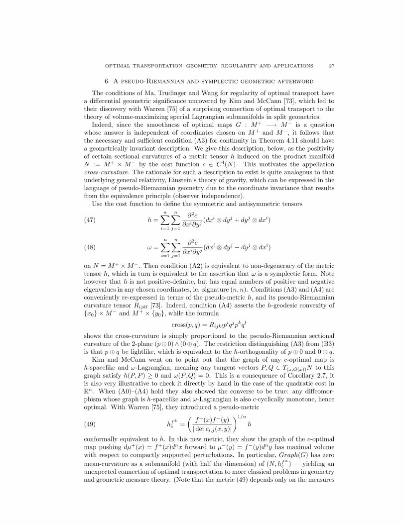
OPTIMAL TRANSPORTATION: GEOMETRY, REGULARITY AND APPLICATIONS 27
6. A pseudo-Riemannian and symplectic geometric afterword
The conditions of Ma, Trudinger and Wang for regularity of optimal transport havea differential geometric significance uncovered by Kim and McCann [73], which led totheir discovery with Warren [75] of a surprising connection of optimal transport to thetheory of volume-maximizing special Lagrangian submanifolds in split geometries.
Indeed, since the smoothness of optimal maps G : M+ −→ M− is a questionwhose answer is independent of coordinates chosen on M+ and M−, it follows thatthe necessary and sufficient condition (A3) for continuity in Theorem 4.11 should havea geometrically invariant description. We give this description, below, as the positivityof certain sectional curvatures of a metric tensor h induced on the product manifoldN := M+ × M− by the cost function c ∈ C4(N). This motivates the appellationcross-curvature. The rationale for such a description to exist is quite analogous to thatunderlying general relativity, Einstein’s theory of gravity, which can be expressed in thelanguage of pseudo-Riemannian geometry due to the coordinate invariance that resultsfrom the equivalence principle (observer independence).
Use the cost function to define the symmetric and antisymmetric tensors
(47) h =n∑
i=1
n∑j=1
∂2c
∂xi∂yj(dxi ⊗ dyj + dyj ⊗ dxi)
(48) ω =n∑
i=1
n∑j=1
∂2c
∂xi∂yj(dxi ⊗ dyj − dyj ⊗ dxi)
on N = M+ ×M−. Then condition (A2) is equivalent to non-degeneracy of the metrictensor h, which in turn is equivalent to the assertion that ω is a symplectic form. Notehowever that h is not positive-definite, but has equal numbers of positive and negativeeigenvalues in any chosen coordinates, ie. signature (n, n). Conditions (A3) and (A4) areconveniently re-expressed in terms of the pseudo-metric h, and its pseudo-Riemanniancurvature tensor Rijkl [73]. Indeed, condition (A4) asserts the h-geodesic convexity of{x0} ×M− and M+ × {y0}, while the formula
cross(p, q) = Rijklpiqjpkql
shows the cross-curvature is simply proportional to the pseudo-Riemannian sectionalcurvature of the 2-plane (p⊕ 0)∧ (0⊕ q). The restriction distinguishing (A3) from (B3)is that p⊕ q be lightlike, which is equivalent to the h-orthogonality of p⊕ 0 and 0⊕ q.
Kim and McCann went on to point out that the graph of any c-optimal map ish-spacelike and ω-Lagrangian, meaning any tangent vectors P,Q ∈ T(x,G(x))N to thisgraph satisfy h(P, P ) ≥ 0 and ω(P,Q) = 0. This is a consequence of Corollary 2.7, itis also very illustrative to check it directly by hand in the case of the quadratic cost inRn. When (A0)–(A4) hold they also showed the converse to be true: any diffeomor-phism whose graph is h-spacelike and ω-Lagrangian is also c-cyclically monotone, henceoptimal. With Warren [75], they introduced a pseudo-metric
(49) hf±
c =(
f+(x)f−(y)|det ci,j(x, y)|
)1/n
h
conformally equivalent to h. In this new metric, they show the graph of the c-optimalmap pushing dµ+(x) = f+(x)dnx forward to µ−(y) = f−(y)dny has maximal volumewith respect to compactly supported perturbations. In particular, Graph(G) has zeromean-curvature as a submanifold (with half the dimension) of (N,hf±
c ) — yielding anunexpected connection of optimal transportation to more classical problems in geometryand geometric measure theory. (Note that the metric (49) depends only on the measures

28 ROBERT J. MCCANN∗ AND NESTOR GUILLEN
f± and the sign of the mixed partial D2xyc in dimension n = 1.) The preprint of Harvey
and Lawson [65] contains a wealth of related information concerning special Lagrangiansubmanifolds in pseudo-Riemannian (= semi-Riemannian) geometry.
References
[1] T. Abdellaoui and H. Heinich. Sur la distance de deux lois dans le cas vectoriel. C.R. Acad. Sci.
Paris Ser. I Math., 319:397–400, 1994.
[2] N. Ahmad, H.K. Kim, and R.J. McCann. Optimal transportation, topology and uniqueness.Preprint at www.math.toronto.edu/mccann.
[3] G. Alberti and L. Ambrosio. A geometrical approach to monotone functions in Rn. Math. Z.,230:259–316, 1999.
[4] L. Ambrosio. Lecture notes on optimal transport problems. In Mathematical Aspects of Evolving
Interfaces, volume 1812 of Lecture Notes in Mathematics, pages 1–52. Springer, Berlin, 2003.[5] L.A. Ambrosio, N. Gigli, and G. Savare. Gradient flows in metric spaces and in the space of
probability measures. Lecture Notes in Mathematics ETH Zurich. Birkhauser Verlag, Basel, 2005.
[6] E.J. Anderson and P. Nash. Linear Programming in Infinite-Dimensional Spaces. Wiley, Chich-ester, 1987.
[7] M. Armstrong. Multiproduct nonlinear pricing. Econometrica, 64:51–75, 1996.
[8] S. Basov. Multidimensional Screening. Springer-Verlag, Berlin, 2005.[9] P. Bernard and B. Buffoni. Optimal mass transportation and Mather theory. J. Eur. Math. Soc.
(JEMS), 9:85–121, 2007.
[10] M. Bernot, V. Caselles, J.-M. Morel. Optimal Transportation Networks: Models and Theories.Springer-Verlag, Berlin, 2009.
[11] S. Bianchini and F. Cavalletti. The Monge problem for distance cost in geodesic spaces. Preprintat http://cvgmt.sns.it/papers/biacav09/[email protected].
[12] G. Bouchitte and G. Buttazzo. Characterization of optimal shapes and masses through Monge-
Kantorovich equation. J. Eur. Math. Soc. (JEMS), 3:139–168, 2001.[13] G. Bouchitte, W. Gangbo and P. Seppecher. Michell trusses and lines of principal action. Math.
Models Methods Appl. Sci., 18:1571–1603, 2008.
[14] Y. Brenier. Decomposition polaire et rearrangement monotone des champs de vecteurs. C.R.Acad. Sci. Paris Ser. I Math., 305:805–808, 1987.
[15] Y. Brenier. Polar factorization and monotone rearrangement of vector-valued functions. Comm.
Pure Appl. Math., 44:375–417, 1991.[16] L. Caffarelli. Allocation maps with general cost functions. In P. Marcellini et al, editor, Partial
Differential Equations and Applications, number 177 in Lecture Notes in Pure and Appl. Math.,
pages 29–35. Dekker, New York, 1996.[17] L.A. Caffarelli. Boundary regularity of maps with convex potentials. Comm. Pure Appl. Math.,
45:1141–1151, 1992.[18] L.A. Caffarelli. The regularity of mappings with a convex potential. J. Amer. Math. Soc., 5:99–
104, 1992.
[19] L.A. Caffarelli. Boundary regularity of maps with convex potentials — II. Ann. of Math. (2),144:453–496, 1996.
[20] L.A. Caffarelli and R.J. McCann. Free boundaries in optimal transport and Monge-Ampere ob-stacle problems. Ann. of Math. (2), 171:673–730, 2010.
[21] L.A. Caffarelli, M. Feldman and R.J. McCann. Constructing optimal maps for Monge’s transportproblem as a limit of strictly convex costs. J. Amer. Math. Soc., 15:1–26, 2002.
[22] G. Carlier. A general existence result for the principal-agent problem with adverse selection. J.Math. Econom., 35:129–150, 2001.
[23] G. Carlier and I. Ekeland. Equilibrium structure of a bidimensional asymmetric city. NonlinearAnal. Real World Appl., 8:725–748, 2008.
[24] J.A. Carrillo, R.J. McCann, and C. Villani. Contractions in the 2-wasserstein length space andthermalization of granular media. Arch. Rational Mech. Anal., 179:217–263, 2006.
[25] T. Champion and L. De Pascale. The Monge problem in Rd. Preprint at
http://cvgmt.sns.it/papers/chadep09/champion-depascale.pdf.
[26] T. Champion, L. De Pascale, and P. Juutinen. The ∞-Wasserstein distance: local solutions andexistence of optimal transport maps. SIAM J. Math. Anal., 40, 2008.
[27] P.-A. Chiappori, R.J. McCann, and L. Nesheim. Hedonic price equilibria, stable matching andoptimal transport: equivalence, topology and uniqueness. Econom. Theory, 42:317–354, 2010.
[28] D. Cordero-Erausquin. Inegalite de Prekopa-Leindler sur la sphere. C.R. Acad. Sci. Paris Ser. I
Math., 329:789–792, 1999.

OPTIMAL TRANSPORTATION: GEOMETRY, REGULARITY AND APPLICATIONS 29
[29] D. Cordero-Erausquin. Sur le transport de mesures periodiques. C.R. Acad. Sci. Paris Ser. I
Math., 329:199–202, 1999.
[30] D. Cordero-Erausquin, R.J. McCann and M. Schmuckenschlager. A Riemannian interpolationinequality a la Borell, Brascamp and Lieb. Invent. Math., 146:219–257, 2001.
[31] D. Cordero-Erausquin, R.J. McCann and M. Schmuckenschlager. Prekopa-Leindler type inequal-
ities on Riemannian manifolds, Jacobi fields, and optimal transport. Ann. Fac. Sci. ToulouseMath. (6), 15:613–635, 2006.
[32] D. Cordero-Erausquin, B. Nazaret, and C. Villani. A mass-transportation approach to sharp
Sobolev and Gagliardo-Nirenberg inequalities. Adv. Math., 182:307–332, 2004.[33] J.A. Cuesta-Albertos and C. Matran. Notes on the Wasserstein metric in Hilbert spaces. Ann.
Probab., 17:1264–1276, 1989.
[34] J.A. Cuesta-Albertos and A. Tuero-Dıaz. A characterization for the solution of the Monge-Kantorovich mass transference problem. Statist. Probab. Lett., 16:147–152, 1993.
[35] M.J.P. Cullen. A Mathematical Theory of Large Scale Atmosphere/Ocean Flows. Imperial CollegePress, London, 2006.
[36] M.J.P Cullen and R.J. Purser. An extended Lagrangian model of semi-geostrophic frontogenesis.
J. Atmos. Sci., 41:1477–1497, 1984.[37] M.J.P Cullen and R.J. Purser. Properties of the Lagrangian semi-geostrophic equations. J. Atmos.
Sci., 46:2684–2697, 1989.
[38] P. Delanoe. Classical solvability in dimension two of the second boundary-value problem associ-ated with the Monge-Ampere operator. Ann. Inst. H. Poincare Anal. Non Lineaire, 8:443–457,
1991.
[39] P. Delanoe and Y. Ge. Regularity of optimal transportation maps on compact, locally nearlyspherical, manifolds. To appear in J. Reine Angew. Math.
[40] R. Dobrushin. Definition of a system of random variables by means of conditional distributions
(Russian). Teor. Verojatnost. i Primenen., 15:469–497, 1970.[41] R.M. Dudley. Probabilities and metrics - Convergence of laws on metric spaces, with a view to
statistical testing. Universitet Matematisk Institut, Aarhus, Denmark, 1976.[42] I. Ekeland. An optimal matching problem. ESAIM: Control, Optimisation and Calculus of Vari-
ations, 11:57–71, 2005.
[43] L.C. Evans. Partial Differential Equations, volume 19 of Graduate Studies in Mathematics. Amer-ican Mathematical Society, Providence, 1998.
[44] L.C. Evans and W. Gangbo. Differential equations methods for the Monge-Kantorovich mass
transfer problem. Mem. Amer. Math. Soc., 137:1–66, 1999.[45] A. Fathi and A. Figalli. Optimal transportation on non-compact manifolds. Israel J. Math.,
175:1–59, 2010.
[46] A. Figalli and N. Gigli. Local seimconvexity of Kantorovich potentials on noncompact manifolds.To appear in ESAIM Control Optim. Calc. Var.
[47] A. Figalli, Y.-H. Kim, and R.J. McCann. Continuity and injectivity of optimal maps for non-
negatively cross-curved costs. Preprint at www.math.toronto.edu/mccann.[48] A. Figalli, Y.-H. Kim, and R.J. McCann. Regularity of optimal transport maps on multiple
products of spheres. Preprint at www.math.toronto.edu/mccann.[49] A. Figalli, Y.-H. Kim, and R.J. McCann. When is multidimensional screening a convex program?
Preprint at www.math.toronto.edu/mccann.
[50] A. Figalli and G. Loeper. C1 regularity of solutions of the Monge-Ampere equation for optimaltransport in dimension two. Calc. Var. Partial Differential Equations, 35:537–550, 2009.
[51] A. Figalli and F. Maggi. On the shape of liquid drops and crystals in the small mass regime.Preprint at http://cvgmt.sns.it/papers/figmag10/fm-small4.pdf.
[52] A. Figalli, F. Maggi and A. Pratelli. A mass transportation approach to quantitative isoperimetric
inequalities. To appear in Invent. Math.
[53] A. Figalli and L. Rifford. Continuity of optimal transport maps on small deformations of S2.Comm. Pure Appl. Math., 62: 1670–1706, 2009.
[54] A. Figalli, L. Rifford and C. Villani. Nearly round spheres look convex. Preprint.[55] A. Figalli, L. Rifford and C. Villani. On the Ma-Trudinger-Wang curvature on surfaces. Preprint.[56] L. Forzani and D. Maldonado. Properties of the solutions to the Monge-Ampere equation. Non-
linear Anal., 57:815–829, 2004.
[57] W. Gangbo. Habilitation thesis. Universite de Metz, 1995.[58] W. Gangbo and R.J. McCann. Optimal maps in Monge’s mass transport problem. C.R. Acad.
Sci. Paris Ser. I Math., 321:1653–1658, 1995.[59] W. Gangbo and R.J. McCann. The geometry of optimal transportation. Acta Math., 177:113–161,
1996.
30 ROBERT J. MCCANN∗ AND NESTOR GUILLEN
[60] W. Gangbo and R.J. McCann. Shape recognition via Wasserstein distance. Quart. Appl. Math.,
58:705–737, 2000.
[61] N. Gigli. On the inverse implication of Brenier-McCann theorems and the structure of(P2(M), W2). Preprint at http://cvgmt.sns.it/papers/gigc/Inverse.pdf.
[62] D. Gilbarg and N.S. Trudinger. Elliptic Partial Differential Equations of Second Order. Springer-
Verlag, New York, 1983.[63] T. Glimm and V. Oliker. Optical design of single reflector systems and the Monge-Kantorovich
mass transfer problem. J. Math. Sci., 117:4096–4108, 2003.
[64] S. Haker, L. Zhu, A. Tannenbaum and S. Angenent. Optimal mass transport for registration andwarping. Int. J. Computer Vision, 60:225–240, 2004.
[65] F.R. Harvey and H.B. Lawson, Jr. Split special Lagrangian geometry. Preprint.
[66] S. Kakutani. A generalization of brouwer’s fixed point theorem. Duke Math. J., 8:457–459, 1941.[67] L. Kantorovich. On the translocation of masses. C.R. (Doklady) Acad. Sci. URSS (N.S.), 37:199–
201, 1942.[68] L. Kantorovich. On a problem of Monge (In Russian). Uspekhi Math. Nauk., 3:225–226, 1948.
[69] L.V. Kantorovich and G.S. Rubinstein. On a space of completely additive functions. Vestnik
Leningrad. Univ., 13:52–59, 1958.[70] H.G. Kellerer. Duality theorems for marginal problems. Z. Wahrsch. Verw. Gebiete, 67:399–432,
1984.
[71] Y.-H. Kim. Counterexamples to continuity of optimal transportation on positively curved Rie-mannian manifolds. Int. Math. Res. Not., Art. ID rnn120:1–15, 2008.
[72] Y.-H. Kim and R.J. McCann. Appendices to original version of Continuity, curvature, and the
general covariance of optimal transportation. Preprint at arXiv:math/0712.3077v1.[73] Y.-H. Kim and R.J. McCann. Continuity, curvature, and the general covariance of optimal trans-
portation. J. Eur. Math. Soc. (JEMS), 12:1009–1040, 2010.
[74] Y.-H. Kim and R.J. McCann. Towards the smoothness of optimal maps on Riemann-ian submersions and Riemannian products (of round spheres in particular). Preprint at
arXiv:math/0806.0351v1 To appear in J. Reine Angew. Math.[75] Y.-H. Kim, R.J. McCann and M. Warren. Pseudo-Riemannian geometry calibrates optimal trans-
portation. Preprint at www.math.toronto.edu/mccann. To appear in Math. Res. Lett.
[76] T.C. Koopmans. Optimum utilization of the transportation system. Econometrica (Supplement),17:136–146, 1949.
[77] P.W.Y. Lee. New computable necessary conditions for the regularity theory of optimal trans-
portation. Preprint at arXiv:0912.4795. To appear in SIAM J. Math. Anal.[78] P.W.Y. Lee and J. Li. New examples on spaces of negative sectional curvature satisfying Ma-
Trudinger-Wang conditions. Preprint at arXiv:0911.3978.
[79] P.W.Y. Lee and R.J. McCann. The Ma-Trudinger-Wang curvature for natural mechanical ac-tions. Preprint at www.math.toronto.edu/mccann. To appear in Calc. Var. Partial Differential
Equations.
[80] V.L. Levin. Abstract cyclical monotonicity and Monge solutions for the general Monge-Kantorovich problem. Set-valued Anal., 7:7–32, 1999.
[81] J. Li. Smooth optimal transportation on hyperbolic space. Master’s thesis, University of Toronto,2009.
[82] J. Liu. Holder regularity of optimal mappings in optimal transportation. Calc Var. Partial Dif-
ferential Equations, 34:435–451, 2009.[83] J. Liu, N.S. Trudinger, X.-J. Wang. Interior C2,α regularity for potential functions in optimal
transportation. Comm. Partial Differential Equations, 35:165–184, 2010.[84] G. Loeper. On the regularity of maps solutions of optimal transportation problems II. The sphere
case and the reflector antenna. To appear in Arch. Ration. Mech. Anal.
[85] G. Loeper. On the regularity of solutions of optimal transportation problems. Acta Math.,
202:241–283, 2009.[86] G. Loeper and C. Villani. Regularity of optimal transport in curved geometry: the non-focal case.
Duke Math. J., 151:431–485, 2010.[87] J. Lott. Optimal transport and Perelman’s reduced volume. Calc. Var. Partial Differential Equa-
tions, 36:49–84, 2009.
[88] J. Lott and C. Villani. Ricci curvature for metric measure spaces via optimal transport. AnnalsMath. (2), 169:903–991, 2009.
[89] X.-N. Ma, N. Trudinger and X.-J. Wang. Regularity of potential functions of the optimal trans-
portation problem. Arch. Rational Mech. Anal., 177:151–183, 2005.[90] F. Maggi and C. Villani. Balls have the worst best Sobolev inequalities. II. Variants and exten-
sions. Calc. Var. Partial Differential Equations, 31:47–74, 2008.

OPTIMAL TRANSPORTATION: GEOMETRY, REGULARITY AND APPLICATIONS 31
[91] R.P. McAfee and J. McMillan. Multidimensional incentive compatibility and mechanism design.
J. Econom. Theory, 46:335–354, 1988.
[92] R.J. McCann. A Convexity Theory for Interacting Gases and Equilibrium Crystals. PhD thesis,Princeton University, 1994.
[93] R.J. McCann. Existence and uniqueness of monotone measure-preserving maps. Duke Math. J.,
80:309–323, 1995.[94] R.J. McCann. A convexity principle for interacting gases. Adv. Math., 128:153–179, 1997.
[95] R.J. McCann. Equilibrium shapes for planar crystals in an external field. Comm. Math. Phys.,
195:699–723, 1998.[96] R.J. McCann. Exact solutions to the transportation problem on the line. R. Soc. Lond. Proc.
Ser. A Math. Phys. Eng. Sci., 455:1341–1380, 1999.
[97] R.J. McCann. Polar factorization of maps on Riemannian manifolds. Geom. Funct. Anal., 11:589–608, 2001.
[98] R.J. McCann. Stable rotating binary stars and fluid in a tube. Houston J. Math., 32:603–632,2006.
[99] R.J. McCann and P. Topping. Ricci flow, entropy, and optimal transportation. Amer. J. Math.,
132:711–730, 2010.[100] R.J. McCann, B. Pass and M. Warren. Rectifiability of optimal transportation plans. Preprint at
www.math.toronto/mccann.
[101] V.D. Milman and G. Schechtman. Asymptotic theory of finite-dimensional normed spaces. Withan appendix by M. Gromov. Springer-Verlag, Berlin, 1986.
[102] George J. Minty. Monotone (nonlinear) operators in hilbert space. Duke Math. J., 29:341–346,
1962.[103] J.A. Mirrlees. An exploration in the theory of optimum income taxation. Rev. Econom. Stud.,
38:175–208, 1971.
[104] G. Monge. Memoire sur la theorie des deblais et de remblais. Histoire de l’Academie Royale desSciences de Paris, avec les Memoires de Mathematique et de Physique pour la meme annee,
pages 666–704, 1781.[105] P.K. Monteiro and F.H. Page Jr. Optimal sellling mechanisms for multiproduct monopolists:
incentive compatibility in the presence of budget constraints. J. Math. Econom., 30:473–502,
1998.[106] M. Mussa and S. Rosen. Monopoly and product quality. J. Econom. Theory, 18:301–317, 1978.
[107] J. von Neumann. Zur Theorie der Gesellschaftsspiele. (German). Math. Ann., 100:295–320, 1928.
[108] J. von Neumann. Uber ein Okonomisches Gleichungssystems und eine Verallgemeinerung dieBrouwerschen Fixpunktsatzes. Ergebuisse eines Mathematischen Seminars, 8:73–83, 1937.
[109] F. Otto. The geometry of dissipative evolution equations: The porous medium equation. Comm.Partial Differential Equations, 26:101–174, 2001.
[110] F. Otto and C. Villani. Generalization of an inequality by Talagrand and links with the logarithmic
Sobolev inequality. J. Funct. Anal., 173:361–400, 2000.[111] B. Pass. Personal communication. 2010.
[112] G. Perelman. The entropy formula for the Ricci flow and its geometric applications. Preprint at
http://arxiv.org/abs/math/0211159.[113] A.Yu. Plakhov. Newton’s problem of the body of minimal averaged resistance (Russian). Mat.
Sb., 195:105–126, 2004.
[114] J. Purser and M.J.P. Cullen. J. Atmos. Sci, 44:3449–3468, 1987.[115] S.T. Rachev and L. Ruschendorf. Mass Transportation Problems. Probab. Appl. Springer-Verlag,
New York, 1998.[116] M.-K. von Renesse and K.-T. Sturm. Transport inequalities, gradient estimates, entropy and
Ricci curvature. Comm. Pure Appl. Math., 58:923–940, 2005.
[117] J.-C. Rochet. A necessary and sufficient condition for rationalizability in a quasi-linear context.J. Math. Econom., 16:191–200, 1987.
[118] J.-C. Rochet and P. Chone. Ironing, sweeping and multidimensional screening. Econometrica,
66:783–826, 1998.[119] R.T. Rockafellar. Characterization of the subdifferentials of convex functions. Pacific J. Math.,
17:497–510, 1966.
[120] L. Ruschendorf. Bounds for distributions with multivariate marginals. In K. Mosler andM. Scarsini, editors, Stochastic Orders and Decision Under Risk, number 19 in IMS Lecture
Notes - Monograph Series, pages 285–310. Institute of Mathematical Statistics, Hayward, CA,
1991.[121] L. Ruschendorf. Optimal solutions of multivariate coupling problems. Appl. Math. (Warsaw),
23:325–338, 1995.
32 ROBERT J. MCCANN∗ AND NESTOR GUILLEN
[122] L. Ruschendorf. On c-optimal random variables. Statist. Probab. Lett., 37:267–270, 1996.
[123] L. Ruschendorf and S.T. Rachev. A characterization of random variables with minimum L2-
distance. J. Multivariate Anal., 32:48–54, 1990.[124] C. Smith and M. Knott. On the optimal transportation of distributions. J. Optim. Theory Appl.,
52:323–329, 1987.
[125] C. Smith and M. Knott. On Hoeffding-Frechet bounds and cyclic monotone relations. J. Multi-variate Anal., 40:328–334, 1992.
[126] M. Spence. Competitive and optimal responses to signals: An analysis of efficiency and distribu-
tion. J. Econom. Theory, 7:296–332, 1974.[127] K.-T. Sturm. On the geometry of metric measure spaces, I and II. Acta Math., 196:65–177, 2006.
[128] V.N. Sudakov. Geometric problems in the theory of infinite-dimensional probability distributions.
Proc. Steklov Inst. Math., 141:1–178, 1979.[129] H. Tanaka. An inequality for a functional of probability distributions and its application to Kac’s
one-dimensional model of a Maxwellian gas. Z. Wahrscheinlichkeitstheorie und Verw. Gebiete,27:47–52, 1973.
[130] P. Topping. L-optimal transportation for Ricci flow. J. Reine Angew. Math., 636:93–122, 2009.
[131] N.S. Trudinger. Isoperimetric inequalities for quermassintegrals. Ann. Inst. H. Poincar Anal. NonLinaire, 11:411–425, 1994.
[132] N.S. Trudinger and X.-J. Wang. On the Monge mass transfer problem. Calc. Var. Paritial Dif-
ferential Equations, 13:19–31, 2001.[133] N.S. Trudinger and X.-J. Wang. On the second boundary value problem for Monge-Ampere type
equations and optimal transportation. Ann. Sc. Norm. Super. Pisa Cl. Sci. (5), 8:1–32, 2009.
[134] N.S. Trudinger and X.-J. Wang. On strict convexity and C1-regularity of potential functions inoptimal transportation. Arch. Rational Mech. Anal., 192:403–418, 2009.
[135] J. Urbas. On the second boundary value problem for equations of Monge-Ampere type. J. Reine
Angew. Math., 487:115–124, 1997.[136] J. Urbas. Mass transfer problems. Lecture Notes, University of Bonn, 1998.
[137] J.A. Viaclovsky. Conformal geometry and fully nonlinear equations. In Phillip A. Griffiths, editor,Inspired by S.S. Chern., volume 11, pages 435–460. World Scientific Publishing Co., Hackensack,
2006.
[138] C. Villani. Topics in Optimal Transportation, volume 58 of Graduate Studies in Mathematics.American Mathematical Society, Providence, 2003.
[139] C. Villani. Optimal Transport. Old and New, volume 338 of Grundlehren der Mathematischen
Wissenschaften [Fundamental Principles of Mathematical Sciences]. Springer, New York, 2009.[140] X.-J. Wang. On the design of a reflector antenna. Inverse Problems, 12:351–375, 1996.
[141] X.-J. Wang. On the design of a reflector antenna II. Calc. Var. Partial Differential Equations,
20:329–341, 2004.[142] L.N. Wasserstein. Markov processes over denumerable products of spaces describing large systems
of automata. Problems of Information Transmission, 5:47–52, 1969.
[143] Q. Xia. The formation of a tree leaf. ESAIM Control Optim. Calc. Var., 13:359–377, 2007.
Department of Mathematics, University of Toronto, Toronto Ontario Canada M5S 2E4
E-mail address: [email protected]
Department of Mathematics, University of Texas at Austin, Austin TX USA 78712E-mail address: [email protected]