fisher consistency for prior probability shift

Journal of Machine Learning Research 18 (2017) 1-32 Submitted 1/17; Revised 4/17; Published 9/17

Fisher Consistency for Prior Probability Shift

Dirk Tasche∗ [email protected]

Swiss Financial Market Supervisory Authority FINMA

Laupenstrasse 27

3003 Bern

Switzerland

Editor: Charles Elkan

Abstract

We introduce Fisher consistency in the sense of unbiasedness as a desirable property forestimators of class prior probabilities. Lack of Fisher consistency could be used as a criterionto dismiss estimators that are unlikely to deliver precise estimates in test data sets underprior probability and more general data set shift. The usefulness of this unbiasednessconcept is demonstrated with three examples of classifiers used for quantification: AdjustedCount, EM-algorithm and CDE-Iterate. We find that Adjusted Count and EM-algorithmare Fisher consistent. A counter-example shows that CDE-Iterate is not Fisher consistentand, therefore, cannot be trusted to deliver reliable estimates of class probabilities.

Keywords: Classification, quantification, class distribution estimation, Fisher consis-tency, data set shift

1. Introduction

The application of a classifier to a test data set often is based on the assumption that thedata for training the classifier is representative of the test data. While this assumptionmight be true sometimes or even most of the time, there may be circumstances when thedistributions of the classes or the features or both are genuinely different in the test set andthe training set. Spam emails represent a familiar example of this situation: The typicalcontents of spam emails and their proportion of the total daily number of emails receivedmay significantly vary over time. Spam email filters developed on the set of emails receivedlast week may become less effective this week due to changes in the composition of theemail traffic. In the machine learning community, this phenomenon is called data set shiftor population drift. The area of research of how to learn a model appropriate for a test seton a differently composed training set is called domain adaptation.

The simplest type of data set shift occurs when the training set and the test set differonly in the distribution of the classes of the instances. In this case, only the prior (orunconditional) class probabilities (or class prevalences) change between the training setand the test set; this type of data set shift is called prior probability shift. In the contextof supervised or semi-supervised learning, the class prevalences in the labelled portion of

∗. The author currently works at the Swiss Financial Market Supervisory Authority (FINMA). The opinionsexpressed in this note are those of the author and do not necessarily reflect views of FINMA.The author thanks the reviewers of this article for suggesting numerous improvements.

c©2017 Dirk Tasche.

License: CC-BY 4.0, see https://creativecommons.org/licenses/by/4.0/. Attribution requirements are providedat http://jmlr.org/papers/v18/17-048.html.

https://creativecommons.org/licenses/by/4.0/

http://jmlr.org/papers/v18/17-048.html

Tasche

the training set are always known. In contrast, the class prevalences in the test set may beknown or unknown at the time of the application of the classifier to the test set, dependingon the cause of the data set shift. For example, in a binary classification exercise theclass prevalence of the majority class in the training set might deliberately be reducedby removing instances of that class at random, in order to facilitate the training of theclassifier. If the original training set were a random sample of the test set then the test setclass prevalences would be equal to the original training set class prevalences and thereforeknown. The earlier mentioned spam email filter problem represents an example of thesituation where the test set class prevalences are unknown due to possible data set shift.

In this paper, we primarily study the question of how to estimate the unknown classprevalences in a test data set when the training set and the test set are related by priorprobability shift. This problem was coined quantification by Forman (2008). Solutions tothe problem are known at least since the 1960s (Gart and Buck, 1966) but research for moreand better solutions has been ongoing ever since. It seems, however, as if the criteria ofwhat should be deemed a ‘good’ solution are not fully clear.

In the words of Cox and Hinkley (1974, p. 287) Fisher consistency is described as“Roughly this requires that if the whole ‘population’ of random variables is observed, thenthe method of estimation should give exactly the right answer”. Obtaining the right answerwhen looking for the value of a parameter is an intuitive concept that exhibits similarity tothe concept of unbiasedness. In particular, if a wrong decision based on the estimated valueof a parameter can entail severe financial loss or cause damage to a person’s health, gettingthe value of the parameter right is very important. Hofer and Krempl (2013) and Tasche(2014) present examples related to the estimation of credit losses. Nonetheless, requiringthat the right answer be obtained also on finite samples from the population would be tooharsh, given that by the nature of randomness the empirical distribution associated with afinite sample can be quite different from the population distribution.

For these reasons, we argue that as a minimum, it should be required that class preva-lence estimators (or quantifiers) be Fisher consistent. Cox and Hinkley (1974, p. 287)comment that “Consistency, however, gives us no idea of the magnitude of the errors of es-timation likely for any given n [the sample size]”. Therefore, being Fisher consistent cannotbe a sufficient criterion for a class prevalence estimator to be useful. Rather, by the logicof a necessary criterion, lack of Fisher consistency should be considered a reason to dismissa candidate estimator. For even for very large sample sizes, with such an estimator therewould not be any guarantee of obtaining an approximation of the true parameter value.

Accordingly, focussing on binary classification and quantification, with this paper wemake three contributions to the literature on quantification of class prevalences:

• We formally introduce the concept of unbiasedness expressed as Fisher consistency, ina prior probability shift context and more generally for quantification of class preva-lences in the presence of any data set shift.

• We illustrate the usefulness of the notion of Fisher consistency, by demonstratingwith three popular quantification approaches that Fisher consistency may be used asa criterion to cull inapt quantifiers. In other words, Fisher consistency can serve as afilter to eliminate quantifiers that are unlikely to provide precise estimates.

2


• We show that Fisher consistency of an estimator is not a global concept that can beexpected to hold for all types of data set shift. To demonstrate this fact, we suggesta new type of data set shift, called ‘invariant density ratio’-type data set shift, whichgeneralises prior probability shift. We also propose a method for generating non-trivialexamples of this type of data set shift.

‘Invariant density ratio’-type data set shift is interesting of its own for the following tworeasons:

• It can be described as a covariate shift without the ‘contamination’ effect that can en-tail the test set class prevalences to be very similar to the training set class prevalences(Tasche, 2013, p. 83).

• Prior probability shift is a special case of ‘invariant density ratio’-type data set shift(see Section 2.4 below). Therefore, estimators which are Fisher consistent with re-spect to ‘Invariant density ratio’-type data set shift potentially have a wider scopeof application than estimators that are Fisher consistent only with respect to priorprobability shift.

In Section 2.4.3, this list is supplemented by a number of other interesting properties of‘invariant density ratio’-type data set shift. The plan for the paper is as follows:

• In Section 2, we recall the concepts from binary classification and quantification thatare relevant for the subject of the paper. These concepts include Bayes classifiers andsome types of data set shift, including prior probability shift. In addition, we motivateand define the notion of Fisher consistency.

• In Section 3, we describe three approaches to class prevalence estimation which serveto illustrate the role of Fisher consistency for this task. The three approaches areAdjusted Count (Forman, 2008), the EM-algorithm (Saerens et al., 2001) and CDE-Iterate (Xue and Weiss, 2009).

• In Section 4, we explore by numerical examples under which circumstances the threeapproaches discussed in Section 3 cease to be Fisher consistent for the estimation ofclass prevalences. The most important finding here is that CDE-Iterate is not Fisherconsistent under prior probability shift. Hence there is no guarantee that CDE-Iteratewill find the true class prevalences even in the presence of that quite benign type ofdata set shift.

• We conclude in Section 5 with some comments on the findings of the paper.

• Appendix A presents some tables with computation results for additional informationwhile Appendix B provides a mathematically rigorous derivation of the equation thatcharacterises the limit of CDE-Iterate.

Notation. Concepts and notation used in this paper are formally introduced where needed.For additional quick reference, here is a short list of the most important symbols:

• X : Feature space.

3

Tasche

• 0, 1: Two classes, 0 positive and 1 negative.

• (X,Y ): X is the vector of the features of an instance, Y denotes the class of theinstance.

• P: Probability distribution of the training set.

• Q: Probability distribution of the test set.

• P[Y = i |X]: Feature-conditional probability of class i in the training set (analogousfor Q).

• P[X ∈ S |Y = i]: P[X |Y ] denotes the class-conditional distribution of the features inthe training set. P[X ∈ S |Y = i] stands for the probability that the realisation of Xis an element of the set S, conditional on the class of the instance being i (analogousfor Q).

• g : X → 0, 1: Classifier that assigns class g(x) to a realisation x of the features ofan instance.

• f0, f1: Class-conditional feature densities on the training set.

• h0, h1: Class-conditional feature densities on the test set.

2. Estimating Prior Probabilities

In this section, we recall some basic concepts from the theory of binary classification andquantification to build the basis for the discussion of prevalence estimation approachesin Section 3 and the numerical examples in Section 4. The concepts discussed includeBayes classifiers and different types of data set shift including prior probability shift and itsextension called here ‘invariant density ratio’-type data set shift. In addition, we introducethe notion of unbiasedness of prevalence estimators in the shape of Fisher consistency whichis most appropriate in the quantification context central for this paper.

2.1 Binary Classification and Bayes Error at Population Level

The basic model we consider is a random vector (X,Y ) with values in a product X ×0, 1of sets. For example, in applications for credit scoring, we might have X = Rd for somepositive integer d. A realisation of X ∈ X is interpreted as the vector of features of anobserved instance. Y ∈ 0, 1 is the class of the observed instance. For the purpose of thispaper, 0 is the interesting (positive) class, as in Hernandez-Orallo et al. (2012).

Classification problem. On the basis of the observed features X of an instance, make aguess (prediction) g(X) ∈ 0, 1 of the instance’s class Y such that the probability of anerror is minimal. In mathematical terms: Find g∗ : X → 0, 1 such that

P[g∗(X) 6= Y ] = ming

P[g(X) 6= Y ]. (1a)

The functions g in (1a) used for predicting Y are called (crisp) classifiers. The value ofthe minimum in (1a) is called Bayes error. (1a) accounts for two possibilities to make

4


classification errors:

‘Predict 0 if the true class is 1’ = g(X) = 0, Y = 1, and

‘Predict 1 if the true class is 0’ = g(X) = 1, Y = 0.

Cost-sensitive errors. In practice, the consequences of these two erroneous predictionsmight have different severities. Say the cost related to ‘predict 0 if the true class is 1’ isc1 ≥ 0, and the cost related to ‘predict 1 if the true class is 0’ is c0 ≥ 0. To deal with theissue of different severities, a cost-sensitive version of (1a) can be studied:

c1 P[g∗(X) = 0, Y = 1] + c0 P[g∗(X) = 1, Y = 0] =

mingc1 P[g(X) = 0, Y = 1] + c0 P[g(X) = 1, Y = 0]. (1b)

To make this problem non-trivial, of course one has to assume that c0 + c1 > 0.Bayes classifier. A solution g∗ to (1b) and therefore also to (1a) (case of c0 = c1 = 1)

exists and is well-known (see Section 2.2 of van Trees, 1968, or Section 1.3 of Elkan, 2001):

g∗(X) =

0, if P[Y = 0 |X] > c1

c0+c1,

1, if P[Y = 0 |X] ≤ c1c0+c1

.(2)

In this equation, P[Y = 0 |X] denotes the (non-elementary) conditional probability ofthe event Y = 0 given X, as defined in standard textbooks on statistical learning andprobability theory (see Appendix A.7 of Devroye et al., 1996, and Section 4.1 of Durrett,1996, respectively). Being a function of X, P[Y = 0 |X] is also a non-constant randomvariable whenever X and Y are not stochastically independent. In the following, we alsocall P[Y = 0 |X] feature-conditional class probability. The function g∗(X) as defined in (2)is called a Bayes classifier.

A proof of (2) is also provided in Appendix B below (see Lemma 5). That proof shows,in particular, that the solution g∗ to (1b) is unique in the sense of P[g∗(X) = g(X)] = 1 forany other minimiser g of (1b), as long as the distribution of the ratio of the class-conditionalfeature densities is continuous (see Section 2.4 for the definition of the density ratio).

2.2 Binary Classification and Bayes Error at Sample Level

In theory, the binary classification problem with cost-sensitive errors is completely solvedin Section 2.1. In practice, however, there are issues that can make the Bayes classifier (2)unfeasible:

• Typically, the joint probability distribution of (X,Y ) is not exactly known but has tobe inferred from a finite sample (called ‘training set’) (x1,tr, y1,tr), . . . , (xm,tr, ym,tr) ∈X × 0, 1. If X is high-dimensional this may be difficult and require a large samplesize to reduce errors due to random variation.

• As the Bayes classifier is explicitly given by (2), one can try to avoid estimatingthe entire distribution of (X,Y ) and, instead, only estimate the feature-conditionalprobability P[Y = 0 |X] (also called posterior probability). However, this task isnot significantly simpler than estimating the distribution of (X,Y ), as illustrated bythe fact that methods for the estimation of non-elementary conditional probabilitiesconstitute a major branch of applied statistics.

5

Tasche

By structural assumptions on the nature of the classification problem (1b), the approachbased on direct estimation of the feature-conditional probability can be rendered more ac-cessible. Logistic regression provides the possibly most important example for this approach(see, e.g., Cramer, 2003). But the price of the underlying assumptions may be high and in-clude significant deterioration of goodness of fit. That is why alternative approaches basedon direct implementation of the optimisation of the right-hand side of (1b) are popular.Lessmann et al. (2015) give a survey of the variety of methods available, just for applicationto credit scoring.

As mentioned in the introduction, one of the topics of this paper is an investigationinto the question of whether certain quantifiers are Fisher consistent. In Section 4 below,the demonstration of lack of Fisher consistency is based on counter-examples which arenon-trivial but simple enough to allow for the exact computation of the feature-conditionalclass probabilities and hence also the Bayes classifiers.

2.3 Data Set Shift

Even if one has succeeded in estimating a Bayes classifier or at least a reasonably goodapproximate Bayes classifier, issues may arise that spoil its effective deployment. Quiteoften, it is assumed that any instance with known features vector x but unknown class ythat is presented for classification has been drawn at random from the same populationas the training set. However, for a number of reasons this assumption can be wrong (see,e.g., Quinonero-Candela et al., 2009; Kull and Flach, 2014; Moreno-Torres et al., 2012;Dal Pozzolo et al., 2015). A lot of research has been undertaken and is ongoing on methodsto deal with this problem of so-called data set shift. In this paper, we consider the followingvariant of the problem:

• There is a training data set (x1,tr, y1,tr), . . . , (xm,tr, ym,tr) ∈ X × 0, 1 which is as-sumed to be an independent and identically distributed sample from the populationdistribution P(X,Y ) of the random vector (X,Y ) as described in Section 2.1.

• There is another data set, the test data set, (x1,te, y1,te), . . . , (xn,te, yn,te) ∈ X ×0, 1which is assumed to be an independent and identically distributed sample from apossibly different population distribution Q(X,Y ). Moreover, training and test datahave been independently generated.

• For the instances in the training data set, their class labels are visible and can bemade use of for learning classifiers (i.e. solving optimisation problem (1b)).

• For the instances in the test data set, their class labels are invisible to us or becomevisible only with large delay.

This assumption is intended to describe a setting where the test instances arrive batch-wise, not as a stream. We also assume that the sizes m of the training set and n of the testset are reasonably large such that trying to infer properties of the respective populationdistributions makes sense.

As far as the theory for this paper is concerned, we will ignore the issues caused bythe fact that we know the training data set distribution P(X,Y ) and the test data set

6


distribution Q(X,Y ) only by inference from finite samples. Instead we will assume that wecan directly deal with the population distributions P(X,Y ) and Q(X,Y ). Throughout thewhole paper, we make the assumption that there are both positive and negative instancesin both of the populations, i.e. it holds that

0 < P[Y = 0] < 1 and 0 < Q[Y = 0] < 1. (3)

The problem that P(X,Y ) and Q(X,Y ) may not be the same is treated under differentnames in the literature (Moreno-Torres et al., 2012): data set shift, domain adaptation,population drift and others. There are several facets of the problem:

• Classifiers may have to be adapted to the test set or re-trained.

• The feature-conditional probabilities may have to be adapted to the test set or re-estimated.

• The unconditional class probabilities (also called prior probabilities or prevalences)may have to be re-adjusted for the test set or re-estimated.

Quantification. In this paper, we focus on the estimation of the prevalences Q[Y = 0]and Q[Y = 1] in the test set, as parameters of distribution Q(X,Y ). This problem iscalled quantification (Forman, 2008) and of its own interest beyond its auxiliary functionfor classification and estimation of the feature-conditional probabilities (Gonzalez et al.,2016).

2.4 Quantification in the Presence of Prior Probability Shift

In technical terms, the quantification problem as presented in Section 2.3 can be describedas follows:

• We know the joint distribution of features and class labels (X,Y ) under the trainingset probability distribution P.

• We know the distribution of the features X under the test set probability distributionQ.

• How can we infer the prevalences of the classes under Q, i.e. the probabilities Q[Y = 0]and Q[Y = 1] = 1−Q[Y = 0], by making best possible use of our knowledge of P(X,Y )and Q(X)?

This question cannot be answered without assuming that the test set probability distributionQ shares some properties with the training set probability distribution P. This means tomake more specific assumptions about the structure of the data set shift between trainingset and test set. In the literature, a variety of different types of data set shift have beendiscussed. See Moreno-Torres et al. (2012), Kull and Flach (2014) or Hofer (2015) for anumber of examples, including ‘covariate shift’ and ‘prior probability shift’ which possiblyare the two most studied types of data set shift. This paper focusses on prior probabilityshift.

7

Tasche

2.4.1 Prior Probability Shift

This type of data set shift also has been called ‘global shift’ (Hofer and Krempl, 2013). Theassumption of prior probability shift is, in particular, appropriate for circumstances wherethe features of an instance are caused by the instance’s class membership (Fawcett andFlach, 2005). Technically, prior probability shift can be described as ‘the class-conditionalfeature distributions of the training and test sets are the same’, i.e.

Q[X ∈ S |Y = 0] = P[X ∈ S |Y = 0] and Q[X ∈ S |Y = 1] = P[X ∈ S |Y = 1], (4)

for all measurable sets S ⊂ X . Note that (4) does not imply Q[X ∈ S] = P[X ∈ S] for allmeasurable S ⊂ X because the training set class distribution P(Y ) and the test set classdistribution Q(Y ) still can be different.

In this paper, we will revisit three approaches to the estimation of the prevalences inpopulation Q in the presence of prior probability shift as defined by (4). Specifically, wewill check both in theory and by simple examples if these three approaches satisfy the basicestimation quality criterion of Fisher consistency. For this purpose, a slight generalisationof prior probability shift called ‘invariant density ratio’-type data set shift will prove useful.Before we introduce it, let us briefly recall some facts on conditional probabilities andprobability densities.

2.4.2 Feature-Conditional Class Probabilities and Class-ConditionalFeature Densities

Typically, the class-conditional feature distributions P(X |Y = i), i = 0, 1, of a data sethave got densities f0 and f1 respectively with respect to some reference measure like thed-dimensional Lebesgue measure. Then also the unconditional feature distribution P(X)has a density f which can be represented as

f(x) = P[Y = 0] f0(x) + (1− P[Y = 0]) f1(x) for all x ∈ X . (5a)

Moreover, the feature-conditional class probability P[Y = 0 |X] can be expressed in termsof the densities f0 and f1:

P[Y = 0 |X](x) =P[Y = 0] f0(x)

P[Y = 0] f0(x) + (1− P[Y = 0]) f1(x), x ∈ X . (5b)

Conversely, assume that there is a density f of the unconditional feature distributionP(X) and the feature-conditional class probability P[Y = 0 |X] is known. Then the class-conditional feature densities f0 and f1 are determined as follows:

f0(x) =P[Y = 0 |X](x)

P[Y = 0]f(x), x ∈ X ,

f1(x) =1− P[Y = 0 |X](x)

1− P[Y = 0]f(x), x ∈ X .

(6)

2.4.3 Invariant Density Ratio

Assume that there are densities f0 and f1 for the class-conditional feature distributionsP(X |Y = i), i = 0, 1, of the training set population. We then say that the data set shift

8


from population P to Q is of ‘invariant density ratio’-type if there are also densities h0 andh1 respectively for the class-conditional distributions Q(X |Y = i), i = 0, 1, of the test set,and it holds that

f0(x)

f1(x)=

h0(x)

h1(x)for all x ∈ X . (7)

Note that by (6), the density ratio f0f1

can be rewritten as

f0(x)

f1(x)=

P[Y = 0 |X](x)

1− P[Y = 0 |X](x)

1− P[Y = 0]

P[Y = 0], x ∈ X , (8)

as long as P[Y = 0 |X](x) < 1. Hence the density ratio can be calculated without knowledgeof the values of the densities if the feature-conditional class probabilities or reasonableapproximations are known.

Obviously, ‘invariant density ratio’ is implied by prior probability shift if all involvedclass-conditional distributions have got densities. ‘Invariant density ratio’-type data setshift was discussed in some detail by Tasche (2014). It is an interesting type of data setshift for several reasons:

1) ‘Invariant density ratio’ extends the concept of prior probability shift.

2) Conceptually, ‘invariant density ratio’ is similiar to covariate shift. To see this recallfirst that covariate shift is defined by the property that the feature-conditional classprobabilities of the training and test sets are the same (Moreno-Torres et al., 2012,Section 4.1):

P[Y = 0 |X] = Q[Y = 0 |X]. (9a)

Then, if there are densities of the class-conditional feature distributions under P andQ like for (7), (9a) can be rewritten as

P[Y = 0]

1− P[Y = 0]

f0(x)

f1(x)=

Q[Y = 0]

1−Q[Y = 0]

h0(x)

h1(x)for all x ∈ X . (9b)

Hence, covariate shift also can be described in terms of the ratio of the class-conditionaldensities, like ‘invariant density ratio’. The two types of data set shift coincide ifP[Y = 0] = Q[Y = 0], i.e. if the class prevalences in the training and test sets are thesame.

3) The maximum likelihood estimates of class prevalences under prior probability shiftactually are maximum likelihood estimates under ‘invariant density ratio’, too (Tasche,2014, p. 152 and Remark 1). Hence they can be calculated with the EM (expectation-maximisation) algorithm as described by Saerens et al. (2001).

4) In terms of the data set shift taxonomy of Moreno-Torres et al. (2012), ‘invariantdensity ratio’ is a non-trivial but manageable ‘other’ shift, i.e. it is neither a prior-probability shift, nor a covariate shift, nor a concept shift.

By properties 1) and 2), ‘invariant density ratio’ has got conceptual similarities with bothprior probability shift and covariate shift. In Section 4 below, we will make use of its man-ageability property 4) to construct an example of data set shift that reveals the limitationsof some common approaches to the estimation of class prevalences.

9

Tasche

2.5 Fisher Consistency

In Section 1, Fisher consistency of an estimator has been described as the property thatthe true value of a parameter related to a probability distribution is recovered when theestimator is applied to the distribution on the whole population. In this section, we applythe notion of Fisher consistency to the quantification of binary class prevalences.

In practice, estimators are often Fisher consistent and asymptotically consistent (weaklyor strongly, see Section 10.4 of van der Vaart, 1998, for the definitions) at the same time.Gerow (1989) discusses the questions of when this is the case and what concept Fisher(1922) originally defined. Our focus on Fisher consistency is not meant to imply thatasymptotic consistency is a less important property. In the context of statistical learning,asymptotic consistency seems to have enjoyed quite a lot of attention, as shown for instanceby the existence of books like Devroye et al. (1996). In addition, the convergence aspectof asymptotic consistency often can be checked empirically by observing the behaviour oflarge samples. However, in some cases it might be unclear if the limit of a seeminglyasymptotically consistent large sample is actually the right one. This is why, thanks to itssimilarity to the concept of unbiasedness which also refers to getting the right value of aparameter, Fisher consistency becomes an important property.

Definition 1 (Fisher consistency) In the data set shift setting of this paper as describedin Section 2.3, we say that an estimator T (Q), applied to the elements Q of a family Q ofpossible population distributions of the test set, is Fisher consistent in Q for the prevalenceof class 0 if it holds that

T (Q) = Q[Y = 0] for all Q ∈ Q. (10)

This definition of Fisher consistency is more restrictive than the definition by Cox and Hink-ley (1974) quoted in Section 1. For it requires the specification of a family of distributionsto which the parameter ‘recovery’ property applies. The family Q of most interest for thepurpose of this paper is the set of distributions Q that are related to one fixed training setdistribution P by prior probability shift, i.e. by (4).

3. Three Approaches to Estimating Class Prevalences under PriorProbability Shift

In this section, we study three approaches to the estimation of binary class prevalences:

• Adjusted Count (AC) (Forman, 2008), called ‘confusion matrix approach’ by Saerenset al. (2001), but in use since long before (Gart and Buck, 1966),

• the EM (expectation maximisation) algorithm by Saerens et al. (2001), describedbefore as maximum likelihood approach by Peters and Coberly (1976), and

• CDE-Iterate (CDE for class distribution estimation) by Xue and Weiss (2009).

A variety of other approaches have been and are being studied in the literature (see thediscussion in Hofer, 2015, for a recent overview). The selection of approaches to be discussedin this paper was driven by findings of Xue and Weiss (2009) and more recently Karpov

10


et al. (2016). According to that research, for the estimation of binary class prevalences theCDE-Iterate approach seems to perform equally well or even stronger than AC which byitself was found to outperform the popular EM-algorithm. In this section, we recall thetechnical details of the approaches which are needed to implement the numerical examplesof Section 4 below.

In addition, we check the three estimators on a theoretical basis for Fisher consistency. Inparticular with regard to CDE-Iterate, the theory is inconclusive with regard to its possibleFisher consistency. However, the example of Section 4.2 below shows that CDE-Iterate isnot Fisher consistent for class 0 prevalence under prior probability shift, in contrast to bothAC and the EM-algorithm.

3.1 Adjusted Count (AC)

Let g : X → 0, 1 be any classifier. Under prior probability shift as described by (4), wethen obtain

Q[g(X) = 0] = Q[Y = 0] Q[g(X) = 0 |Y = 0] + (1−Q[Y = 0]) Q[g(X) = 0 |Y = 1]

= Q[Y = 0] P[g(X) = 0 |Y = 0] + (1−Q[Y = 0]) P[g(X) = 0 |Y = 1]. (11)

If P[g(X) = 0 |Y = 0] 6= P[g(X) = 0 |Y = 1], i.e. if g(X) and Y are not stochasticallyindependent, (11) is equivalent to

Q[Y = 0] =Q[g(X) = 0]− P[g(X) = 0 |Y = 1]

P[g(X) = 0 |Y = 0]− P[g(X) = 0 |Y = 1]. (12)

Equation (12) is called the AC approach to the quantification of binary class prevalences.Let us recall some useful facts about AC:

• Equation (12) has been around for a long time, at least since the 1960s. In this paper,the quantification approach related to (12) is called ‘Adjusted Count’ as in Forman(2008) because this term nicely describes what is done.

• Q[g(X) = 0] is the proportion of instances in the test set (measured by counting) thatare classified (predicted) positive by classifier g(X).

• P[g(X) = 0 |Y = 1] is the ‘false positive rate’, as measured for classifier g(X) on thetraining set.

• P[g(X) = 0 |Y = 0] is the ‘true positive rate’, as measured for classifier g(X) on thetraining set.

• Forman (2008) discusses AC in detail and provides a number of variations of the themein order to account for its deficiencies.

• Possibly, the main issue with AC is that in practice the result of the right-hand sideof (12) can turn out to be negative or greater than 1. This can happen for one ormore of the following reasons:

1. The data set shift in question actually is no prior probability shift, i.e. (4) doesnot hold.

11

Tasche

2. The estimates of the true positive and true negative rates are inaccurate.

3. The estimation of the scoring function underlying the classifier from limitedtraining data may be inaccurate (both biased and subject to high variance).

• In theory, if the data set shift is indeed a prior probability shift, the result of theright-hand side of (12) should be the same, regardless of which admissible (i.e. suchthat the denominator is not zero) classifier is deployed for determining the proportionof instances in the test set classified positive. Hence, whenever in practice differentclassifiers give significantly different results, that could suggest that the assumptionof prior probability shift is wrong.

• As long as g(X) and Y are at least somewhat dependent, possible lack of power of theclassifier g should not be an issue for the applicability of (12) because the denominatoron the right-hand side of (12) is then different from zero.

For a training set distribution P denote by Qprior = Qprior(P) the family of distributions Qthat are related to P by prior probability shift in the sense of Definition 1, i.e.

Qprior = Q : Q is probability measure satisfying (4). (13)

Then, for fixed training set distribution P and fixed classifier g(X) such that g(X) and Y arenot independent under P, the AC approach is Fisher consistent in Qprior for the prevalenceof class 0 by construction: Define the operator T = Tg,P by

T (Q) =Q[g(X) = 0]− P[g(X) = 0 |Y = 1]

P[g(X) = 0 |Y = 0]− P[g(X) = 0 |Y = 1].

Then (12) implies (10) for Q ∈ Qprior. However, denote—again for some fixed training setdistribution P—by Qinvariant = Qinvariant(P) the family of distributions Q that are relatedto P by ‘invariant density ratio’-type data set shift in the sense of (7), i.e.

Qinvariant = Q : Q is probability measure satisfying (7). (14)

Then in general the AC approach is not Fisher consistent in Qinvariant. For it is shown inSection 4.3 below that there are a classifier g∗, a distribution P∗ and a related distributionQ∗ ∈ Qinvariant(P

∗) such that

Tg∗,P∗(Q∗) 6= Q∗[Y = 0].

3.2 EM-Algorithm

Saerens et al. (2001) made the EM-algorithm popular for the estimation of class prevalences,as a necessary step for the re-adjustment of thresholds of soft classifiers. A closer inspectionof the article by Peters and Coberly (1976) shows that they actually had studied the samealgorithm and provided conditions for its convergence. In particular, this observation againdraws attention to the fact that the EM-algorithm, deployed on data samples, should resultin unique maximum likelihood estimates of the class prevalences.

As noticed by Du Plessis and Sugiyama (2014), the population level equivalent of samplelevel maximum likelihood estimation of the class prevalences under an assumption of prior

12


probability shift is minimisation of the Kullback-Leibler distance between the estimated testset feature distribution and the observed test set feature distribution. Moreover, Tasche(2014) observed that the EM-algorithm finds the true values of the class prevalences not onlyunder prior probability shift but also under ‘invariant density ratio’-type data set shift. Inother words, the EM-algorithm is Fisher consistent both in Qprior and Qinvariant, as definedin (13) and (14) respectively, for the prevalence of class 0. See Proposition 2 below for aformal proof.

In the case of two classes, the maximum-likelihood version of the EM-algorithm in thesense of solving the likelihood equation is more efficient than the EM-algorithm itself. Thisstatement applies even more to the population level calculations. In this paper, therefore,we describe the result of the EM-algorithm as the unique solution of a specific equation, aspresented in Tasche (2014).

3.3 Calculating the Result of the EM-Algorithm.

In the population setting of Section 2.3 with training set distribution P(X,Y ) and test setdistribution Q(X,Y ), assume that the class-conditional feature distributions P(X |Y = i),i = 0, 1, of the training set have got densities f0 and f1. Define the density ratio R by

R(x) =f0(x)

f1(x), for x ∈ X . (15)

We then define the estimation operator TR(Q) for the prevalence of class 0 as the uniquesolution q ∈ (0, 1) of the equation (Tasche, 2014)

0 = EQ

[R(X)− 1

1 + q (R(X)− 1)

], (16a)

where EQ denotes the expectation operator with respect to Q. Unfortunately, not alwaysdoes a solution of (16a) exist in (0, 1). There exists a solution in (0, 1) if and only if

EQ[R(X)] > 1 and EQ

[1

R(X)

]> 1, (16b)

and if there is a solution in (0, 1) it is unique (Tasche, 2014, Remark 2(a)).

Proposition 2 The operator TR(Q) (EM-algorithm), as defined by (16a), is Fisher con-sistent in Qprior and Qinvariant for the prevalence of class 0.

Proof We only have to prove the claim for Qinvariant because Qprior is a subset of Qinvariant.Let any Q ∈ Qinvariant be given and denote by hi, i = 0, 1, its class-conditional featuredensities. By (7) and (5b), it then follows that

EQ

[R(X)− 1

1 + Q[Y = 0] (R(X)− 1)

]= EQ

[h0 − h1

h1 + Q[Y = 0] (h0 − h1)

]=

EQ

[Q[Y = 0 |X]

]Q[Y = 0]

−EQ

[Q[Y = 1 |X]

]Q[Y = 1]

= 1− 1 = 0.

13

Tasche

Hence, the prevalence Q[Y = 0] of class 0 is a solution of (16a) and, therefore, the onlysolution. As a consequence, TR(Q) is well-defined and satisfies TR(Q) = Q[Y = 0].

In practice, for fixed q the right-hand side of (16a) could be estimated on a test setsample (x1,te, y1,te), . . ., (xn,te, yn,te) as in Section 2.3 by the sample average

1

n

n∑i=1

R(xi,te)− 1

1 + q (R(xi,te)− 1),

where R could be plugged in as a training set estimate of the density ratio by means of (8).

3.4 CDE-Iterate

In order to successfully apply the AC quantification approach as described in Section 3.1,we must get hold of reliable estimates of the training set true and false positive rates ofthe classifier deployed. If the positive class is the minority class, the estimation of the truepositive rate can be subject to large uncertainties and hence may be hard to achieve withsatisfactory accuracy. Similarly, if the negative class is the minority class, the estimation ofthe false positive rate can be rather difficult.

Application of the EM-algorithm as introduced by Saerens et al. (2001) or described inSection 3.2 requires reliable estimation of the feature-conditional class probabilities or thedensity ratio. Again, such estimates in general are hard to achieve. That is why alternativemethods for quantification are always welcome. In particular, methods that are basedexclusively on learning one or more crisp classifiers are promising. For learning classifiersis a well-investigated problem for which efficient solution approaches are available (see, forinstance, Lessmann et al., 2015, for a survey related to credit scoring).

Xue and Weiss (2009) proposed ‘CDE-Iterate’ (CDE for class distribution estimation)which is appropriately summarised by Karpov et al. (2016) as follows: “The main idea ofthis method is to retrain a classifier at each iteration, where the iterations progressivelyimprove the quantification accuracy of performing the ‘classify and count’ method via thegenerated cost-sensitive classifiers.” Xue and Weiss motivated the CDE-Iterate algorithmas kind of an equivalent of the EM-algorithm, with the training set feature-conditional classprobabilities replaced by Bayes classifiers (or approximations of the Bayes classifiers) learnton the training set.

In this paper, we do not retrain a classifier but make use of the fact that we have gota closed-form representation of the optimal classifier resulting from the retraining, by (2).Taking this into account and using notation adapted for this paper, we obtain the followingdescription of the CDE-Iterate procedure:

CDE-Iterate algorithm

1) Set initial parameters: k = 0, c(0)0 = 1, c

(0)1 = 1.

2) Find Bayes classifier under training distribution P(X,Y ):

gk(X) =

0, if P[Y = 0 |X] >

c(k)1

c(k)0 +c

(k)1

,

1, if P[Y = 0 |X] ≤ c(k)1

c(k)0 +c

(k)1

.

14


3) Under test feature distribution Q(X) compute qk = Q[gk(X) = 0].

4) Increment k by 1.

5) Reset cost parameters: c(k)1 =

1−qk−1

1−P[Y=0] , c(k)0 =

qk−1

P[Y=0] .

6) If convergence is reached or k = kmax then stop, and accept qk−1 as the CDE-Iterateestimate of Q[Y = 0]. Else continue with step 2.

Xue and Weiss (2009) did not provide a proof of convergence or unbiasedness for CDE-Iterate. In Section 6 of their paper, they state that “one improvement would be to adaptthe CDE-Iterative method to automatically terminate once the class distribution estimateconverges. This might improve overall performance over any specific CDE-Iterate-n methodand would eliminate the problem of identifying the appropriate number of iterations. It ispossible that such a CDE-converge method would outperform CDE-AC.” In this paper, weprove convergence of CDE-Iterate and also show that it does not outperform ‘CDE-AC’(Adjusted Count in the notation of this paper) for class distribution estimation under priorprobability shift, thus answering the quoted research questions of Xue and Weiss.

The proof of the convergence of CDE-Iterate as described above is provided in Propo-sition 6 in Appendix B below. There it is also shown that the limit q∗ = limk→∞ qk solvesthe following equation1:

q∗ =

Q[R(X) ≥ 1−q∗

q∗

], if q0 ≥ q1 and qk > q∗ for all k,

Q[R(X) > 1−q∗

q∗

], otherwise,

(17)

where R(x) is defined by (15).

The limit result (17) is quite general in so far as it is not based on any assumption withregard to the type of data set shift between the training set distribution P(X,Y ) and thetest set distribution Q(X,Y ). If we restrict the type of data set shift to prior probabilityshift or ‘invariant density ratio’-type data set shift as defined in Section 2.4, does (17) thenimply Fisher consistency for the prevalence of class 0 in either of these two families ofdistributions? As we show by example in the following section, the answer to this questionis ‘no’.

4. Numerical Examples

In Section 3, we have found that AC as an estimator of class prevalences is Fisher consistentfor prior probability shift while the EM-algorithm is even Fisher consistent for the moregeneral ‘invariant density ratio’-type data set shift. We have not yet answered the questionif CDE-Iterate is Fisher consistent for either of these two data set shift types.

The property of an estimator to be Fisher consistent is something that has to be proved.In contrast, lack of Fisher consistency of an estimator is conveniently shown by providinga counter-example. This is the purpose of the following subsections: We show by examplesthat

1. Subject to the technical condition that P(X) has a density f such that Q[f(X) > 0] = 1.

15

Tasche

• CDE-Iterate is not Fisher consistent for prior probability shift (and hence for ‘invariantdensity ratio’-type data set shift neither),

• AC is not Fisher consistent for ‘invariant density ratio’-type data set shift, and

• the EM-algorithm is no longer Fisher consistent if the ‘invariant density ratio’-typedata set shift is slightly modified.

We present the counter-examples as a simulation and estimation experiment that is executedfor each of the three following example models:

• Section 4.2: Binormal model with equal variances for both training and test set (priorprobability shift).

• Section 4.3: Binormal model with equal variances for training set and model with non-normal class-conditional densities but identical density ratio for test set (‘invariantdensity ratio’-type data set shift).

• Section 4.4: Binormal model with equal variances for training set and model withnon-normal class-conditional densities and a different density ratio for test set (neitherprior probability shift nor ‘invariant density ratio’-type data set shift).

The experimental design is described in Section 4.1 below. The classical binormal modelwith equal variances has been selected as the training set model for the following reasons:

• Logistic regression finds the correct feature-conditional class probabilities.

• Needed algorithms are available in common software packages like R.

• The ratio of the class-conditional feature densities has a particularly simple shape,see (21b) below.

• The binormal model with equal variances has been found useful before for a similarexperiment (Tasche, 2016).

Thresholds for Bayes classifier under data set shift. We deploy the logistic regression ascoded by R Core Team (2014). Therefore, it is convenient to always use the feature-conditional class-probability P[Y = 0 |X] as the Bayes classifier, both for the training setand for the test set after a possible data set shift (then with a modified threshold). In orderto be able to do so, we observe that, under prior probability shift or even ‘invariant densityratio’-type data set shift, the test set Bayes classifier gtest(X) for the cost-sensitive errorcriterion (1b) can be represented both as

gtest(X)(2)=

0, if Q[Y = 0 |X] > c1

c0+c1,

1, if Q[Y = 0 |X] ≤ c1c0+c1

,

16


and as (see Saerens et al., 2001, Section 2.2)

gtest(X) =

0, if P[Y = 0 |X] >c1

1−Q[Y=0]1−P[Y=0]

c11−Q[Y=0]1−P[Y=0] + c0

Q[Y=0]P[Y=0]

,

1, if P[Y = 0 |X] ≤c1

1−Q[Y=0]1−P[Y=0]

c11−Q[Y=0]1−P[Y=0] + c0

Q[Y=0]P[Y=0]

.

(18)

4.1 Design of the Experiment

In the subsequent sections 4.2, 4.3 and 4.4, we conduct the following experiment and reportits results2:

• For a given training set (sample and population) represented by distribution P(X,Y ),we determine the Bayes classifier that is optimal for minimising the Bayes error(1a). We represent the Bayes classifier by a decision threshold applied to the feature-conditional probability of class 0 as in (2), with c0 = 1 = c1.

• We create test sets (by simulation or as population distribution), represented by dis-tributions Q(X,Y ), which are related to the training set by certain types of data setshift, including prior probability shift and ‘invariant density ratio’-type data set shift.

• On the test sets, we deploy three different quantification methods for the estimationof the prevalence of class 0 (see also Definition 3 below): CDE-Iterate (defined inSection 3.4), Adjusted Count (defined in Section 3.1), and EM-algorithm (defined inSection 3.2).

• Based on the estimated class 0 prevalences, we adapt the threshold of the Bayesclassifier according to (18) such that it would be optimal for minimising the Bayes error(equivalently for maximising the classification accuracy) if the estimated prevalencewere equal to the true test set class 0 prevalence and the test set were related to thetraining set by prior probability shift or by ‘invariant density ratio’-type data set shift.

• We report the following results for samples and populations:

– Classification accuracy and F-measure (see (23a) and (23b) for the definitions) ofthe adapted Bayes classifier when applied to the test set, because these measureswere used by Xue and Weiss (2009).

– Estimated prevalences of class 0, for direct comparison of estimation results andtrue values.

– Relative error: If q is the true probability and q the estimated probability, thenwe tabulate

max

(|q − q|q

,|1− q − (1− q)|

1− q

)=

|q − q|min(q, 1− q)

. (19)

2. The R-scripts used for creating the tables and figures of this paper can be received upon request fromthe author.

17

Tasche

Relative error behaves similar to Kullback-Leibler distance used by Karpov et al.(2016), but is defined also for q = 0 and q = 1 and, moreover, has a more intuitiveinterpretation.

Modelled class prevalences. The setting is broadly the same as for the artificial data set inKarpov et al. (2016). For each model, we consider a training set with class probabilities50%, combined with test sets with class 0 probabilities 1%, 5%, 10%, 30%, 50%, 70%, 90%,95% and 99%. For the samples as well as for the population distributions, we deploy theestimation approaches whose acronyms are given in the following definition to estimate thetest set class 0 prevalences.

Definition 3 (Acronyms for estimation approaches)The following estimation approaches are used in this section:

• CDE-Iterate in three variants:

– CDE1: First iteration of the algorithm described in Section 3.4. Identical withClassify & Count of Forman (2008).

– CDE2: Second iteration of the algorithm described in Section 3.4.

– CDE∞: CDE-Iterate converged, as described in Section 3.4.

• AC: Adjusted Count as described in Section 3.1.

• EM: EM-algorithm as described in Section 3.2.

4.2 Training Set: Binormal; Test Set: Binormal

We consider the classical binormal model with equal variances as an example that fits wellinto the prior probability shift setting of Section 2.4. We specify the binormal model bydefining the class-conditional feature distributions.

• Training set: Both class-conditional feature distributions are normal, with equal vari-ances, i.e.

P(X |Y = 0) = N (µ, σ2), P(X |Y = 1) = N (ν, σ2), (20a)

with µ < ν and σ > 0.

• Test set: Same as training set.

• For this section’s numerical experiment, the following parameter values have beenchosen:

µ = 0, ν = 2, σ = 1. (20b)

For the sake of brevity, in the following we sometimes refer to the setting of this sectionas ‘double’ binormal. The feature-conditional class probability P[Y = 0 |X] in the trainingset is given by

P[Y = 0 |X](x) =1

1 + exp(a x+ b), x ∈ R, (21a)

18


with a = ν−µσ2 > 0 and b = µ2−ν2

2σ2 + log(1−P[Y=0]P[Y=0]

). For the density ratio R according to

(15), we obtain

R(x) = exp(x µ−ν

σ2 + ν2−µ22σ2

), x ∈ R. (21b)

For the sample version of the example in this section, we create by Monte-Carlo simu-lation a training sample

((x1,tr, y1,tr), . . . , (xm,tr, ym,tr)

)∈ (R × 0, 1)m and test samples(

(x1,te, y1,te), . . . , (xn,te, yn,te))∈ (R × 0, 1)n with class-conditional feature distributions

given by (20a) that approximate the training set population distribution P and the test setpopulation distributions Q as described in general terms in Section 2.4 and more specificallyhere by (20a), (20b) and the respective class 0 prevalences.

• In principle, (x1,tr, y1,tr), . . . , (xm,tr, ym,tr) is an independent and identically distributed(iid) sample from P as specified by (20a), (20b) and ‘training’ class 0 prevalenceP[Y = 0] = 0.5.

• In principle, (x1,te, y1,te), . . . , (xn,te, yn,te) is an iid sample from Q as specified by(20a), (20b) and ‘test’ class 0 prevalences Q[Y = 0] ∈ 0.01, 0.05, 0.1, 0.3, 0.5, 0.7, 0.9,0.95, 0.99.

• However, following the precedent of Xue and Weiss (2009), for both data sets we haveused stratified sampling such that the proportion of (xi,tr, yi,tr) with yi,tr = 0 in thetraining set is exactly P[Y = 0], and the proportion of (xi,te, yi,te) with yi,te = 0 inthe test set is exactly Q[Y = 0].

The sample sizes for both the training and the test set samples have been chosen to be10,000, i.e.

m = n = 10, 000. (22)

In our experimental design, the sampling is conducted mainly for illustration purposesbecause at the same time we also calculate the results at population (i.e. sample size ∞)level such that we know the theoretical outcomes. Therefore, for each parametrisation ofeach model, there is no repeated sampling, i.e. only one sample is created.

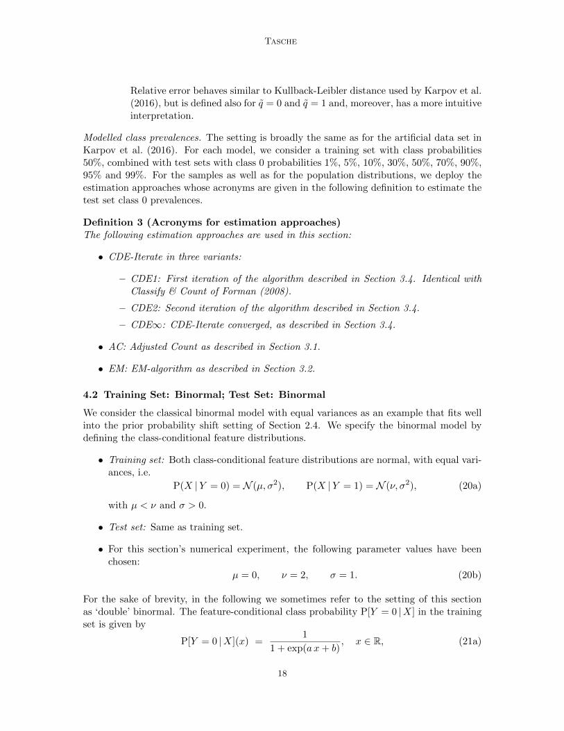
Table 1 shows the class 0 prevalence estimates made in the double binormal setting ofthis section. Note that in the lower panel of the table, the population estimates by AC andEM are exact—as they should be since in Sections 3.1 and 3.2 we have proved that bothestimators are Fisher consistent for the prevalence of class 0 in the family of prior probabilityshifted distributions. The numbers from the lower panel also show that, in general, neitherof the three CDE-Iterate3 variants CDE1, CDE2 and CDE∞ are Fisher consistent for class0 prevalence under prior probability shift, except for the case of identical training and testset distributions.

As mentioned in Section 2.1, in the setting of the binormal model with equal variances,the Bayes classifier is unique, irrespective of its specific representation. Hence, in thisexample, there is no chance to work-around the lack of Fisher consistency for CDE-Iterateby trying to find alternative Bayes classifiers.

3. Note that in any case the tabulated estimates by CDE1, CDE2 and CDE∞ confirm the monotonicitystatement in Proposition 6 of Appendix B for the convergence of CDE-Iterate.

19

Tasche

Q[Y=0] 0.01 0.05 0.10 0.30 0.50 0.70 0.90 0.95 0.99

Prevalence estimates on samples

CDE1 0.1637 0.1910 0.2288 0.3639 0.4989 0.6351 0.7720 0.8014 0.8356

CDE2 0.0402 0.0682 0.1127 0.2991 0.4986 0.7014 0.8851 0.9230 0.9619

CDE∞ 0.0000 0.0000 0.0040 0.2416 0.4985 0.7653 0.9929 1.0000 1.0000

AC -0.0010 0.0391 0.0947 0.2935 0.4921 0.6924 0.8938 0.9370 0.9873

EM 0.0070 0.0475 0.0968 0.2988 0.4967 0.6981 0.9007 0.9467 0.9890

Prevalence estimates on populations

CDE1 0.1655 0.1928 0.2269 0.3635 0.5000 0.6365 0.7731 0.8072 0.8345

CDE2 0.0406 0.0715 0.1131 0.2994 0.5000 0.7006 0.8869 0.9285 0.9594

CDE∞ 0.0000 0.0000 0.0121 0.2389 0.5000 0.7611 0.9879 1.0000 1.0000

AC 0.0100 0.0500 0.1000 0.3000 0.5000 0.7000 0.9000 0.9500 0.9900

EM 0.0100 0.0500 0.1000 0.3000 0.5000 0.7000 0.9000 0.9500 0.9900

Table 1: Class 0 prevalence estimates on the test sets. Training set: Binormal with equalvariances. Test sets: Binormal with equal variances. ‘Q[Y=0]’ is the true test setprevalence of class 0. See Definition 3 for the other acronyms.

However, from the sample estimation numbers in the upper panel of Table 1, we canconclude that in practice CDE2 may provide estimates of the class 0 prevalence that arebetter or at least not much worse than the AC and EM estimates. Table 4 in Appendix Awith the relative errors of the estimates confirms this observation. Such incidences couldexplain the favourable performance of CDE-Iterate observed by Xue and Weiss (2009) andKarpov et al. (2016).

For the sake of completeness, in Tables 5 and 6 in Appendix A, we report the classi-fication accuracies and F-measures respectively, for the training set Bayes classifier withadapted thresholds according to (18), computed on the different test sets. The metricsclassification accuracy and F-measure here are of interest because Xue and Weiss (2009)used them for measuring the performance of the classifiers discussed in their study. Forany classifier g : X → 0, 1, we make use of the following population level formulae forclassification accuracy and F-measure:

Classification accuracy = 1− Classification Error = Q[g(X) = Y ], (23a)

F-measure =2× Recall× Precision

Recall + Precision

=2 Q[g(X) = 0 |Y = 0] Q[Y = 0 | g(X) = 0]

Q[g(X) = 0 |Y = 0] + Q[Y = 0 | g(X) = 0]. (23b)

In these formulae, Q is used to indicate the test set probability distribution in accordancewith the general assumption of this paper.

Basically, Tables 5 and 6 in Appendix A demonstrate that it is hard to draw conclu-sions on quantification performance by looking at classification accuracy or F-measure as

20


−2 0 2 4

0.0

0.1

0.2

0.3

0.4

Feature value

De

nsity

Class 0 trainingClass 1 trainingClass 0 testClass 1 test

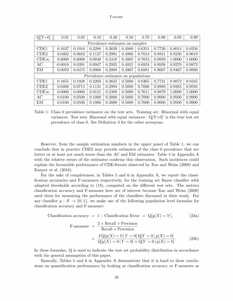
Figure 1: Training set and test set class-conditional densities for Section 4.3. The ratio ofthe training set densities and the ratio of the test set densities are equal.

performance metrics. Both at sample and at population level, the tabulated classificationaccuracy values of CDE∞, AC and EM are almost indistinguishable. While the slightlybetter accuracy values for EM-algorithm and AC compared to CDE∞ at population levelare indeed sure evidence of better performance, the better values at sample level mightjust be random effects. A similar statement applies to the F-measure values of CDE2, ACand EM. The NaNs in Table 6 are caused by zero and negative estimates of the class 0prevalence.

4.3 Training Set: Binormal; Test Set: Non-normal Densities, BinormalDensity Ratio

The combination of a binormal model with equal variances for the training set and a modelwith the same density ratio but non-normal class-conditional feature distributions providesan example that fits conveniently into the ‘invariant density ratio’-type data set shift settingof Section 2.4. We again specify the two models by their class-conditional feature densities.

Training set. Both class-conditional feature distributions are normal, with equal vari-ances, as specified in (20a) and (20b).

Test set. We specify the test set distribution by class-conditional feature densities h0and h1 chosen in such a way that their ratio h0(x)

h1(x), x ∈ R, is given by (21b). Then it equals

the feature density ratio in the double binormal model from Section 4.2. In addition, we

21

Tasche

require that the resulting model is easy to handle numerically but still not too close to thedouble binormal model. To achieve this, we apply the following steps:

• We start with a normal density h∗ characterised by the parameters

Mean = ϑ, variance = τ2 > 0. (24a)

For the purpose of this paper, we have chosen

ϑ = 0.5, τ = 1.4. (24b)

• Then we apply Theorem 3 of Tasche (2014) to decompose h∗ into a mixture q∗ h0 +

(1− q∗)h1 of h0 and h1, subject to the condition h0(x)h1(x)

= exp(x µ−ν

σ2 + ν2−µ22σ2

), x ∈ R,

with µ, ν and σ given by (20b). The important step for the decomposition is todetermine q∗. This can be done as suggested in Section 3.2, by solving a version ofEquation (16a) for the variable q:

0 =

∫ ∞−∞

R(x)− 1

1 + q (R(x)− 1)h∗(x) dx, (25a)

where R(x) is given by (21b). There is a unique solution 0 < q = q∗ < 1 if and only if∫R(x)h∗(x) dx > 1 and

∫R(x)−1 h∗(x) dx > 1.

With parameters set as in (20b) and (24b), the solution for q is

q∗ = 0.7239184.

• If q∗ denotes the solution of (25a) the resulting class conditional feature densities aredetermined as

h0(x) =R(x)h∗(x)

1 + q∗ (R(x)− 1)and h1(x) =

h∗(x)

1 + q∗ (R(x)− 1), x ∈ R. (25b)

Once the densities h0 and h1 have been made available by (25b), the test set class-conditionalfeature distributions Q(X |Y = 0) and Q(X |Y = 1) can be defined as the distributionsdetermined by these densities. Figure 1 shows the test set class-conditional densities from(25b) and the normal densities related to the training set.

For the population-related calculations and the sample simulations, we use the samplesizes as specified in (22), training set class 0 prevalence P[Y = 0] = 0.5 and test setclass 0 prevalences Q[Y = 0] ∈ 0.01, 0.05, 0.1, 0.3, 0.5, 0.7, 0.9, 0.95, 0.99 as in the doublebinormal case of Section 4.2. Again, the samples are stratified with separate sampling fromclasses 0 and 1. This is straightforward for the binormal model of the training set, but lessstraightforward for the test set distributions given by the class-conditional densities (25b).For this sampling we have applied the simple accept-reject algorithm described in Robertand Casella (2004, Corollary 2.17).

22


Q[Y=0] 0.01 0.05 0.10 0.30 0.50 0.70 0.90 0.95 0.99


CDE1 0.1548 0.1865 0.2207 0.3526 0.4931 0.6136 0.7508 0.7850 0.8161

CDE2 0.0313 0.0644 0.1014 0.2773 0.4901 0.6736 0.8728 0.9228 0.9542

CDE∞ 0.0001 0.0010 0.0236 0.2084 0.4848 0.7462 0.9994 1.0000 1.0000

AC -0.0141 0.0325 0.0828 0.2768 0.4835 0.6608 0.8626 0.9129 0.9587

EM 0.0074 0.0467 0.0957 0.2932 0.4994 0.6853 0.8990 0.9503 0.9913


CDE1 0.1641 0.1907 0.2240 0.3572 0.4904 0.6236 0.7568 0.7901 0.8167

CDE2 0.0359 0.0653 0.1049 0.2855 0.4853 0.6890 0.8794 0.9217 0.9531

CDE∞ 0.0000 0.0032 0.0264 0.2168 0.4794 0.7731 1.0000 1.0000 1.0000

AC 0.0080 0.0470 0.0958 0.2908 0.4859 0.6810 0.8761 0.9249 0.9639

EM 0.0100 0.0500 0.1000 0.3000 0.5000 0.7000 0.9000 0.9500 0.9900

Table 2: Class 0 prevalence estimates on the test sets. Training set: Binormal with equalvariances. Test sets: Non-normal densities, binormal density ratio. ‘Q[Y=0]’ isthe true test set prevalence of class 0. See Definition 3 for the other acronyms.

Table 2 shows the class 0 prevalence estimates made in the ‘binormal – non-binormalwith binormal density ratio’ setting of this section. In the lower panel of the table, thepopulation estimates by EM are exact—as they should be since in Section 3.2 we haveproved that the EM-algorithm is Fisher consistent for the prevalence of class 0 in the familyof test set distributions subject to ‘invariant density ratio’-type data set shift. The numbersfrom the lower panel also show that, in general, neither AC nor any of the three CDE-Iterate variants CDE1, CDE2 and CDE∞ are Fisher consistent for class 0 prevalence under‘invariant density ratio’-type data set shift, not even in the case of training and test setswith equal class 0 prevalences. However, while the performance of CDE∞ and CDE1 isreally poor, CDE2 at least is not worse than AC in this setting.

This observation is confirmed by looking at the relative error table 7 in Appendix A andthe upper ‘sample’ panel of Table 2. Hence, outside of the prior probability setting, CDE2may well outperform AC. The ‘sample’ error figures also demonstrate that while in theorythe EM-algorithm should deliver unbiased estimates of the class 0 test set prevalence under‘invariant density ratio’-type data set shift, in practice for extreme prevalences like 1% or99% the estimation error may be significant also for the EM-algorithm.

Since we have already seen in Section 4.2 that measurements of accuracy and F-measureare not very helpful for assessing quantification accuracy, we do not present them for themodel of this section.

4.4 Training Set: Binormal; Test Set: Non-normal Densities, Non-binormalDensity Ratio

The setting of this section for the training and test set distributions is exactly the same asin Section 4.3, with the exception that the ratio h0

h1of the class-conditional feature densities

23

Tasche

−2 0 2 4

0.0

0.1

0.2

0.3

0.4

Feature value

De

nsity

Class 0 trainingClass 1 trainingClass 0 testClass 1 test

Figure 2: Training set and test set class-conditional densities for Section 4.4. The ratio ofthe test set densities is equal to the square root of the ratio of the training setdensities.

is not equal to the test set density as given by (21b) but to its square root:

h0(x)

h1(x)=√R(X) = exp

(2x (µ− ν) + ν2 − µ2

4σ2

). (26)

Otherwise, the class-conditional feature densities h0 and h1 are again determined by thesolution of (25a) and (25b) (with R(x) replaced by

√R(X)). This time, the solution for q

is

q∗ = 0.8152434.

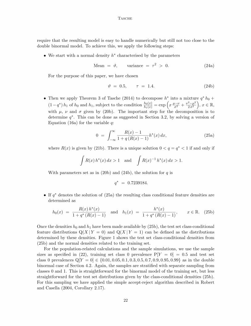
Figure 2 shows the test set class-conditional densities from (25b) and the normal densitiesrelated to the training set in this case. Also the sample simulations are conducted in thesame way as in Section 4.3, again with an accept-reject algorithm deployed for the test setsimulations.

Table 3 and Table 8 in Appendix A show that the EM-algorithm is no longer Fisherconsistent for the prevalence of class 0 when the test set distribution under considerationhas not been generated from the training set distribution by ‘invariant density ratio’-typedata set shift. Unsurprisingly, given that AC is not Fisher consistent on test sets whichare not generated by prior probability shift, it is not Fisher consistent in the family oftest set distributions generated by this modified ‘invariant density ratio’-type data set shift

24


Q[Y=0] 0.01 0.05 0.10 0.30 0.50 0.70 0.90 0.95 0.99


Q[Y=0] 0.01 0.05 0.10 0.30 0.50 0.70 0.90 0.95 0.99

CDE1 0.2593 0.2766 0.3015 0.3987 0.4926 0.5774 0.6697 0.7007 0.7124

CDE2 0.1458 0.1666 0.2033 0.3428 0.4883 0.6196 0.7596 0.8083 0.8221

CDE∞ 0.0001 0.0321 0.0920 0.2812 0.4830 0.6612 0.8993 0.9786 0.9998

AC 0.1396 0.1650 0.2017 0.3447 0.4828 0.6075 0.7433 0.7889 0.8061

EM 0.1274 0.1505 0.1952 0.3448 0.4946 0.6251 0.7785 0.8295 0.8482


CDE1 0.2664 0.2850 0.3081 0.4008 0.4934 0.5861 0.6788 0.7019 0.7205

CDE2 0.1512 0.1775 0.2109 0.3486 0.4899 0.6320 0.7715 0.8055 0.8324

CDE∞ 0.0000 0.0398 0.0914 0.2886 0.4859 0.6875 0.9020 0.9681 1.0000

AC 0.1579 0.1850 0.2189 0.3547 0.4904 0.6261 0.7619 0.7958 0.8230

EM 0.1307 0.1627 0.2015 0.3500 0.4947 0.6394 0.7875 0.8259 0.8576

Table 3: Class 0 prevalence estimates on the test sets. Training set: Binormal with equalvariances. Test sets: Non-normal densities, non-binormal density ratio. ‘Q[Y=0]’is the true test set prevalence of class 0. See Definition 3 for the other acronyms.

either. While both CDE1 and CDE2 perform really poorly in this section’s model setting,CDE∞ performs better, both at sample and at population level. At sample level, even theCDE∞-estimates of the small class 0 prevalences look sensible.

5. Conclusions

In this paper, we have discussed the notion of Fisher consistency as a basic unbiasednessrequirement for class prevalence quantifiers in the presence of data set shift. The usefulnessof Fisher consistency has been demonstrated with three examples of classifiers serving asquantifiers: Adjusted Count, EM-algorithm, and CDE-Iterate. We have shown by examplethat CDE-Iterate is not Fisher consistent even for simple prior probability shift. AdjustedCount and EM-algorithm are Fisher consistent for prior probability shift but lose this prop-erty under data set shifts deviating not much from prior probability shift. Hence beforerelying on prevalence estimates by Adjusted Count or EM-algorithm, users should carefullycheck what kind of data set shift they are confronted with. As a further contribution toquantification-related research, we have suggested a method, based on the concept of ‘in-variant density ratio’-type data set shift, for conveniently generating non-trivial data setshift beyond prior probability shift and covariate shift but conceptually close to both ofthese types of data set shift.

25

Tasche

Appendix A. Additional Tables

Q[Y=0] 0.01 0.05 0.10 0.30 0.50 0.70 0.90 0.95 0.99

Relative error of prevalence estimates on samples

CDE1 15.3700 2.8200 1.2880 0.2130 0.0022 0.2163 1.2800 2.9720 15.4400

CDE2 3.0200 0.3640 0.1270 0.0030 0.0028 0.0047 0.1490 0.5400 2.8100

CDE∞ 1.0000 1.0000 0.9600 0.1947 0.0030 0.2177 0.9290 1.0000 1.0000

AC 1.1030 0.2174 0.0527 0.0218 0.0159 0.0253 0.0621 0.2592 0.2651

EM 0.2987 0.0496 0.0321 0.0040 0.0065 0.0064 0.0073 0.0657 0.1042

Relative error of prevalence estimates on populations

CDE1 15.5482 2.8558 1.2692 0.2115 0.0000 0.2115 1.2692 2.8558 15.5482

CDE2 3.0631 0.4304 0.1311 0.0019 0.0000 0.0019 0.1311 0.4304 3.0631

CDE∞ 1.0000 1.0000 0.8789 0.2038 0.0000 0.2038 0.8789 1.0000 1.0000

AC 0.0000 0.0000 0.0000 0.0000 0.0000 0.0000 0.0000 0.0000 0.0000

EM 0.0000 0.0000 0.0000 0.0000 0.0000 0.0000 0.0000 0.0000 0.0000

Table 4: Relative error of class 0 prevalence estimates on the test sets. Training set: Bi-normal with equal variances. Test sets: Binormal with equal variances. ‘Q[Y=0]’is the true test set prevalence of class 0. See Definition 3 for the other acronyms.

Q[Y=0] 0.01 0.05 0.10 0.30 0.50 0.70 0.90 0.95 0.99

Classification accuracy on samples

CDE1 0.9598 0.9414 0.9139 0.8581 0.8430 0.8606 0.9141 0.9334 0.9615

CDE2 0.9868 0.9591 0.9255 0.8610 0.8431 0.8614 0.9223 0.9581 0.9882

CDE∞ 0.9900 0.9500 0.9040 0.8594 0.8431 0.8573 0.9069 0.9500 0.9900

AC 0.9900 0.9591 0.9266 0.8612 0.8427 0.8617 0.9230 0.9593 0.9903

EM 0.9905 0.9592 0.9265 0.8609 0.8434 0.8613 0.9240 0.9599 0.9903

Classification accuracy on populations

CDE1 0.9609 0.9397 0.9170 0.8591 0.8413 0.8591 0.9170 0.9397 0.9609

CDE2 0.9879 0.9588 0.9297 0.8613 0.8413 0.8613 0.9297 0.9588 0.9879

CDE∞ 0.9900 0.9500 0.9109 0.8589 0.8413 0.8589 0.9109 0.9500 0.9900

AC 0.9905 0.9595 0.9299 0.8613 0.8413 0.8613 0.9299 0.9595 0.9905

EM 0.9905 0.9595 0.9299 0.8613 0.8413 0.8613 0.9299 0.9595 0.9905

Table 5: Classification accuracy on the test sets. Training set: Binormal with equal vari-ances. Test sets: Binormal with equal variances. ‘Q[Y=0]’ is the true test setprevalence of class 0. See Definition 3 for the other acronyms.

26


Q[Y=0] 0.01 0.05 0.10 0.30 0.50 0.70 0.90 0.95 0.99

F-measure on samples

CDE1 0.1992 0.5042 0.5952 0.7631 0.8428 0.9005 0.9519 0.9644 0.9803

CDE2 0.2143 0.4723 0.5509 0.7561 0.8429 0.9033 0.9576 0.9781 0.9940

CDE∞ NaN NaN 0.0769 0.7404 0.8429 0.9026 0.9508 0.9744 0.9950

AC NaN 0.4029 0.5360 0.7552 0.8420 0.9032 0.9581 0.9788 0.9951

EM 0.0952 0.4270 0.5380 0.7559 0.8431 0.9031 0.9587 0.9792 0.9951

F-measure on populations

CDE1 0.2274 0.5035 0.6106 0.7649 0.8413 0.8994 0.9536 0.9679 0.9799

CDE2 0.3174 0.4855 0.5815 0.7562 0.8413 0.9030 0.9617 0.9785 0.9939

CDE∞ NaN NaN 0.2050 0.7382 0.8413 0.9034 0.9528 0.9744 0.9950

AC 0.1697 0.4404 0.5681 0.7563 0.8413 0.9030 0.9619 0.9790 0.9952

EM 0.1697 0.4404 0.5681 0.7563 0.8413 0.9030 0.9619 0.9790 0.9952

Table 6: Classifier F-measure on the test sets. Training set: Binormal with equal variances.Test sets: Binormal with equal variances. ‘Q[Y=0]’ is the true test set prevalenceof class 0. See Definition 3 for the other acronyms.

Q[Y=0] 0.01 0.05 0.10 0.30 0.50 0.70 0.90 0.95 0.99


CDE1 14.4800 2.7300 1.2070 0.1753 0.0138 0.2880 1.4920 3.3000 17.3900

CDE2 2.1300 0.2880 0.0140 0.0757 0.0198 0.0880 0.2720 0.5440 3.5800

CDE∞ 0.9900 0.9800 0.7640 0.3053 0.0304 0.1540 0.9940 1.0000 1.0000

AC 2.4122 0.3498 0.1718 0.0772 0.0330 0.1307 0.3739 0.7417 3.1336

EM 0.2638 0.0667 0.0433 0.0227 0.0012 0.0489 0.0096 0.0056 0.1325


CDE1 15.4091 2.8146 1.2402 0.1907 0.0192 0.2547 1.4324 3.1988 17.3302

CDE2 2.5914 0.3051 0.0490 0.0483 0.0295 0.0367 0.2059 0.5655 3.6945

CDE∞ 1.0000 0.9355 0.7365 0.2774 0.0411 0.2437 1.0000 1.0000 1.0000

AC 0.2038 0.0604 0.0425 0.0305 0.0281 0.0633 0.2389 0.5024 2.6102

EM 0.0029 0.0000 0.0000 0.0000 0.0000 0.0001 0.0000 0.0001 0.0010

Table 7: Relative error of class 0 prevalence estimates on the test sets. Training set: Bi-normal with equal variances. Test sets: Non-normal densities, binormal densityratio. ‘Q[Y=0]’ is the true test set prevalence of class 0. See Definition 3 for theother acronyms.

27

Tasche

Q[Y=0] 0.01 0.05 0.10 0.30 0.50 0.70 0.90 0.95 0.99


CDE1 24.9300 4.5320 2.0150 0.3290 0.0148 0.4087 2.3030 4.9860 27.7600

CDE2 13.5800 2.3320 1.0330 0.1427 0.0234 0.2680 1.4040 2.8340 16.7900

CDE∞ 0.9900 0.3580 0.0800 0.0627 0.0340 0.1293 0.0070 0.5720 0.9800

AC 12.9600 2.3010 1.0168 0.1489 0.0344 0.3082 1.5669 3.2218 18.3881

EM 11.7408 2.0095 0.9518 0.1495 0.0108 0.2497 1.2146 2.4093 14.1813


CDE1 25.6419 4.6990 2.0812 0.3359 0.0131 0.3796 2.2122 4.9611 26.9524

CDE2 14.1179 2.5494 1.1085 0.1618 0.0201 0.2268 1.2851 2.8896 15.7629

CDE∞ 1.0000 0.2049 0.0863 0.0381 0.0281 0.0418 0.0204 0.3618 1.0000

AC 14.7852 2.7000 1.1893 0.1822 0.0192 0.2462 1.3813 3.0839 16.7047

EM 12.0686 2.2549 1.0149 0.1667 0.0105 0.2019 1.1254 2.4814 13.2365

Table 8: Relative error of class 0 prevalence estimates on the test sets. Training set: Binor-mal with equal variances. Test sets: Non-normal densities, non-binormal densityratio. ‘Q[Y=0]’ is the true test set prevalence of class 0. See Definition 3 for theother acronyms.

Appendix B. Proof of the Convergence of CDE-Iterate

In order to provide a fully rigorous proof of Equation (17) that characterises the limit ofCDE-Iterate, we adopt measure-theoretic notation in this section. See standard textbookson probability theory like Billingsley (1995) or Durrett (1996) for reference.

We discuss the problem in a ‘mixture model’ probabilitistic context specified by thefollowing assumption.

Assumption 4 P0 and P1 are probability measures on some measurable space (Ω,H). BothP0 and P1 are absolutely continuous with respect to some measure µ on (Ω,H). The densityof Pi with respect to µ is fi, i = 0, 1.

Note that in the setting of Sections 2 and 3.4, Assumption 4 is satisfied when the trainingset class-conditional feature distributions have got densities. Choose in that case Ω = X ,P0[H] = P[X ∈ H |Y = 0] and P1[H] = P[X ∈ H |Y = 1]. The σ-fieldH is any appropriateσ-field on X , for instance the Borel-σ-field in case X = Rd.

For events H ∈ H we denote the complement of H in Ω by Hc, i.e. we have Hc = Ω\H.Then, in the setting of this section, crisp classifiers g(X) with values 0 or 1 are describedas events by the relations g(X) = 0 = H and g(X) = 1 = Hc.

The following lemma translates the optimisation problem (1b) and its solution (2) intothis section’s notation and enhances them with a statement on the uniqueness of the solu-tion.

Lemma 5 Let a0, a1 ≥ 0. Under Assumption 4, then for all H ∈ H, it holds that

a0 P0[Hc] + a1 P1[H] ≥ a0 P0[a1 f1 ≥ a0 f0] + a1 P1[a1 f1 < a0 f0]. (27)

28


Equality in (27) holds if and only if 0 = µ(H ∩ a1 f1 > a0 f0

)and 0 = µ

(Hc ∩ a1 f1 <

a0 f0).

Proof We inspect the following chain of equations and inequalities:

a0 P0[Hc] + a1 P1[H] = a0 + a1 P1[H]− a0 P0[H]

= a0 +

∫Ha1 f1 − a0 f0 dµ

= a0 +

∫H∩a1 f1<a0 f0

a1 f1 − a0 f0 dµ+

∫H∩a1 f1>a0 f0

a1 f1 − a0 f0 dµ

a)

≥ a0 +

∫H∩a1 f1<a0 f0

a1 f1 − a0 f0 dµ

b)

≥ a0 +

∫a1 f1<a0 f0

a1 f1 − a0 f0 dµ

= a0 P0[a1 f1 ≥ a0 f0] + a1 P1[a1 f1 < a0 f0].

This proves (27). By inequality a), equality in (27) implies 0 =∫H∩a1 f1>a0 f0 a1 f1 −

a0 f0 dµ and, therefore, 0 = µ(H ∩ a1 f1 > a0 f0

). Similarly, equality in (27) implies

0 = µ(Hc ∩ a1 f1 < a0 f0

)because of inequality b).

Lemma 5 characterises the solutions H∗ of the optimisation problem

a0 P0[(H∗)c] + a1 P1[H

∗] = minH∈H a0 P0[Hc] + a1 P1[H]. (28)

One solution is the event a1 f1 < a0 f0 ∈ H. However, the solution is not unique. Forinstance, a1 f1 ≤ a0 f0 ∈ H is another solution as it easily can be checked that the twoconditions for equality in (27) are satisfied. If we have µ(a1 f1 = a0 f0) = 0, then theminimising event a1 f1 < a0 f0 from Lemma 5 is unique in the following sense: If H∗ ∈ His another minimising event then it follows that4

0 = µ(∆(H∗, a1 f1 < a0 f0)

)= µ

((H∗)c ∩ a1 f1 < a0 f0

)+ µ

(H∗ ∩ a1 f1 < a0 f0c

).

Hence H∗ and a1 f1 < a0 f0 are almost everywhere equal.Assume, similarly to Section 2.3, that there is another probability measure Q on (Ω,H).

Q is interpreted as the unconditional distribution of the features on a test set whose classdistribution is (not yet) known. In the notation of this section, then the CDE-Iteratealgorithm of Xue and Weiss (2009) can be described as follows:

CDE-Iterate algorithm

1) Set initial parameters: k = 0, a(0)0 > 0, a

(0)1 > 0.

2) Find optimal classifier under Assumption 4: Hk = a(k)1 f1 < a(k)0 f0.

4. For two sets A and B, the term ∆(A,B) denotes the set difference ∆(A,B) = ((A ∩Bc) ∪ (Ac ∩B).

29

Tasche

3) Under probability Q compute qk = Q[Hk].

4) Increment k by 1.

5) Reset cost parameters: a(k)0 = qk−1, a

(k)1 = 1− qk−1.

6) If convergence is reached or k = kmax then stop, else continue with step 2).

Convergence of the CDE-algorithm as given above or in the paper by Xue and Weiss (2009)is not obvious. However, we can state the following result.

Proposition 6 Under Assumption 4, the sequence (qk)k≥0 determined by the CDE-algorithmas described in this section converges for any probability measure Q on (Ω,H) and any choice

of the intial parameters a(0)0 > 0 and a

(0)1 > 0. The limit q∗ = limk→∞ qk satisfies the equa-

tion

q∗ =

Q[(1− q∗) f1 ≤ q∗ f0, f0 + f1 > 0

], if q0 ≥ q1 and qn > q∗ for all k.

Q[(1− q∗) f1 < q∗ f0

], otherwise.

(29)

Proof Suppose that qk ≤ qk+1 for some k. Then it follows that

qk+2 = Q[(1− qk+1) f1 < qk+1 f0

]= Q

[f1 < qk+1 (f0 + f1)

]≥ Q

[(1− qk) f1 < qk f0

]= qk+1.

Hence (qk)k≥0 is non-decreasing if q0 ≤ q1. Similarly, it can be shown that (qk)k≥0 isnon-increasing if q0 ≥ q1. It follows that q∗ = limk→∞ qk exists.

Note that Q[f1 < x (f0 + f1)

]= Q[f0 + f1 > 0] Q

[ f1f0+f1

< x | f0 + f1 > 0]

is theleft-continuous version of a distribution function. Therefore, it follows that

limy↑x Q[f1 < y (f0 + f1)

]= Q

[f1 < x (f0 + f1)

],

limy↓x Q[f1 < y (f0 + f1)

]= Q

[f1 ≤ x (f0 + f1), f0 + f1 > 0

]By definition of qk, this implies (29).

References

P. Billingsley. Probability and measure. John Wiley & Sons, third edition, 1995.

D.R. Cox and D.V. Hinkley. Theoretical Statistics. Chapman and Hall, 1974.

J.S. Cramer. Logit Models From Economics and Other Fields. Cambridge University Press,2003.

A. Dal Pozzolo, O. Caelen, R.A. Johnson, and G. Bontempi. Calibrating Probability withUndersampling for Unbalanced Classification. In 2015 IEEE Symposium Series on Com-putational Intelligence, pages 159–166. IEEE, 2015.

30


L. Devroye, L. Gyorfi, and G. Lugosi. A Probabilistic Theory of Pattern Recognition.Springer, 1996.

M.C. Du Plessis and M. Sugiyama. Semi-supervised learning of class balance under class-prior change by distribution matching. Neural Networks, 50:110–119, 2014.

R. Durrett. Probability: Theory and Examples. Duxbury Press, second edition, 1996.

C. Elkan. The foundations of cost-sensitive learning. In B. Nebel, editor, SeventeenthInternational Joint Conference on Artificial Intelligence, IJCAI 2001, pages 973–978.Morgan Kaufmann, 2001.

T. Fawcett and P.A. Flach. A response to Webb and Ting’s On the Application of ROCAnalysis to Predict Classification Performance under Varying Class Distributions. Ma-chine Learning, 58(1):33–38, 2005.

R.A. Fisher. On the Mathematical Foundations of Theoretical Statistics. PhilosophicalTransactions of the Royal Society of London, Series A, 222:309–368, 1922.

G. Forman. Quantifying counts and costs via classification. Data Mining and KnowledgeDiscovery, 17(2):164–206, 2008.

J.J. Gart and A.A. Buck. Comparison of a screening test and a reference test in epidemio-logic studies. II. A probabilistic model for the comparison of diagnostic tests. AmericanJournal of Epidemiology, 83(3):593–602, 1966.

K. Gerow. Fisher Consistency – the Evolution of a Concept: It’s Hard to Get It Right theFirst Time. Technical Report BU-1022-M, Cornell University, Biometrics Unit, 1989.

P. Gonzalez, J. Dıez, N. Chawla, and J.J. del Coz. Why is quantification an interestinglearning problem? Progress in Artificial Intelligence, pages 1–6, 2016.

J. Hernandez-Orallo, P. Flach, and C. Ferri. A unified view of performance metrics: Trans-lating threshold choice into expected classification loss. Journal of Machine LearningResearch, 13:2813–2869, 2012.

V. Hofer. Adapting a classification rule to local and global shift when only unlabelled dataare available. European Journal of Operational Research, 243(1):177–189, 2015.

V. Hofer and G. Krempl. Drift mining in data: A framework for addressing drift in classi-fication. Computational Statistics & Data Analysis, 57(1):377–391, 2013.

N. Karpov, A. Porshnev, and K. Rudakov. NRU-HSE at SemEval-2016 Task 4: Com-parative Analysis of Two Iterative Methods Using Quantification Library. In 10thInternational Workshop on Semantic Evaluation (SemEval-2016), pages 171–177, SanDiego, California, June 2016. Association for Computational Linguistics. URL http:

//www.aclweb.org/anthology/S16-1025.

M. Kull and P. Flach. Patterns of dataset shift. In First International Workshop on Learningover Multiple Contexts (LMCE) at ECML-PKDD, 2014.

31

http://www.aclweb.org/anthology/S16-1025

http://www.aclweb.org/anthology/S16-1025

Tasche

S. Lessmann, B. Baesens, H.-V. Seow, and L.C. Thomas. Benchmarking state-of-the-artclassification algorithms for credit scoring: An update of research. European Journal ofOperational Research, 247(1):124–136, 2015.

J.G. Moreno-Torres, T. Raeder, R. Alaiz-Rodriguez, N.V. Chawla, and F. Herrera. Aunifying view on dataset shift in classification. Pattern Recognition, 45(1):521–530, 2012.

C. Peters and W.A. Coberly. The numerical evaluation of the maximum-likelihood estimateof mixture proportions. Communications in Statistics – Theory and Methods, 5(12):1127–1135, 1976.

J. Quinonero-Candela, M. Sugiyama, A. Schwaighofer, and N.D. Lawrence, editors. Datasetshift in machine learning. MIT Press, 2009.

R Core Team. R: A Language and Environment for Statistical Computing. R Foundationfor Statistical Computing, Vienna, Austria, 2014. URL http://www.R-project.org/.

C.P. Robert and G. Casella. Monte Carlo Statistical Methods. Springer-Verlag, secondedition, 2004.

M. Saerens, P. Latinne, and C. Decaestecker. Adjusting the Outputs of a Classifier to Newa Priori Probabilities: A Simple Procedure. Neural Computation, 14(1):21–41, 2001.

D. Tasche. The art of probability-of-default curve calibration. Journal of Credit Risk, 9(4):63–103, 2013.

D. Tasche. Exact fit of simple finite mixture models. Journal of Risk and Financial Man-agement, 7(4):150–164, 2014.

D. Tasche. Does quantification without adjustments work? arXiv preprintarXiv:1602.08780, 2016.

A.W. van der Vaart. Asymptotic Statistics. Cambridge University Press, 1998.

H.L. van Trees. Detection, Estimation, and Modulation Theory, Part I. John Wiley & Sons,1968.

J.C. Xue and G.M. Weiss. Quantification and Semi-supervised Classification Methods forHandling Changes in Class Distribution. In 15th ACM SIGKDD International Conferenceon Knowledge Discovery and Data Mining, pages 897–906, New York, 2009.

32

http://www.R-project.org/

fisher consistency for prior probability shift

Documents