fish assemblage dynamics and red drum habitat selection …
TRANSCRIPT

University of New Orleans University of New Orleans
ScholarWorks@UNO ScholarWorks@UNO
University of New Orleans Theses and Dissertations Dissertations and Theses
Spring 5-18-2012
Fish Assemblage Dynamics and Red Drum Habitat Selection in Fish Assemblage Dynamics and Red Drum Habitat Selection in
Bayou St. John and Associated Urban Waterways located within Bayou St. John and Associated Urban Waterways located within
the City of New Orleans, Louisiana the City of New Orleans, Louisiana
Patrick W. Smith Mr. University of New Orleans
Follow this and additional works at: https://scholarworks.uno.edu/td
Part of the Aquaculture and Fisheries Commons, Behavior and Ethology Commons, Biodiversity
Commons, Marine Biology Commons, and the Other Ecology and Evolutionary Biology Commons
Recommended Citation Recommended Citation Smith, Patrick W. Mr., "Fish Assemblage Dynamics and Red Drum Habitat Selection in Bayou St. John and Associated Urban Waterways located within the City of New Orleans, Louisiana" (2012). University of New Orleans Theses and Dissertations. 1485. https://scholarworks.uno.edu/td/1485
This Thesis is protected by copyright and/or related rights. It has been brought to you by ScholarWorks@UNO with permission from the rights-holder(s). You are free to use this Thesis in any way that is permitted by the copyright and related rights legislation that applies to your use. For other uses you need to obtain permission from the rights-holder(s) directly, unless additional rights are indicated by a Creative Commons license in the record and/or on the work itself. This Thesis has been accepted for inclusion in University of New Orleans Theses and Dissertations by an authorized administrator of ScholarWorks@UNO. For more information, please contact [email protected].

Fish Assemblage Dynamics and Red Drum Habitat Selection in Bayou St. John and Associated
Urban Waterways located within the City of New Orleans, Louisiana
A Thesis
Submitted to the Graduate Faculty of the
University of New Orleans
in partial fulfillment of the
requirements for the degree of
Master of Science
in
Earth and Environmental Science
by
Patrick Smith
B.Sc. Augusta State University, 2008
May 2012

ii
Dedication
I dedicate this manuscript to my wife, Greer Smith. I could not have done this without
her love and support. Thank you for your support and understanding.

iii
Acknowledgments
Many people helped me throughout this process. First, I would like to thank my Advisor,
Dr. Martin T. O’Connell, for accepting me into his lab and all of the hard work since. I would
also like to thank my committee members, Dr. R. Glenn Thomas and Dr. Michael D. Kaller, for
their support and guidance along the way. I am very appreciative of Sunny Brogan for all her
help since I took over this project. Many people within the Nekton Research Lab have helped
along the way with field and analytical work including: Chris Schieble, Will Stein, Jenny Wolfe,
Chris Davis, Jon McKenzie, Dr. Tom Lorenz, Angela Williamson, Arnaud Kerisit, Celeste
Espinido, Shane Abeare, Miadah Bader, and Iain Kelly. Several volunteers have helped
throughout this process; I would like to especially thank Anthony Armato for his hard work and
endless enthusiasm. I would also like to thank my family for their support and understanding
during this process.

iv
Table of Contents
List of Figures……………………………………………………………………………………..v
List of Tables…………………………………………………………………………………….vii
Abstract…...………………………………………………………………………………………ix
Chapter 1…………………………………………………………………………………………..1
Introduction………………………………………………………………………………..1
Materials and Methods…………………………………………………………………….7
Results……………………………………………………………………………………15
Discussion………………………………………………………………………………..44
Conclusions………………………………………………………………………………49
Chapter 2…………………………………………………………………………........................51
Introduction………………………………………………………………………………51
Materials and Methods…………………………………………………………………...55
Results……………………………………………………………………………………61
Discussion………………………………………………………………………………..84
Conclusions………………………………………………………………………………88
References………………………………………………………………………………………..90
Appendix I-IACUC Approval…………..………………………………………………………..96
Vita……………………………………………………………………………………………….97

v
List of Figures
Figure 1-Bayou St. John…………………………………………………………………………..8
Figure 2-Bayou St. John Sites……………………………………………………………………..9
Figure 3-Collinearity of Predictor Variables…………………………………………………….12
Figure 4- Number of Pings per Day per Site…………………………………………………….16
Figure 5-Mud Crab Abundance by Site September – December 2010……………………….....18
Figure 6-Mud Crab Abundance by Site May 2010 – May 2011………………………………...19
Figure 7-Daily Mean Temperature………………………………………………………………22
Figure 8-Daily Mean Salinity……………………………………………………………………23
Figure 9-Daily Mean Depth……………………………………………………………………...24
Figure 10-Daily Mean Dissolved Oxygen……………………………………………………….25
Figure 11-REL Pings vs. Temperature Mathematical…………………………………………...29
Figure 12-REL Pings vs. Salinity Mathematical………………………………………………...30
Figure 13-REL Pings vs. Dissolved Oxygen Mathematical……………………………………..31
Figure 14-NEI Pings vs. Temperature Mathematical……………………………………………32
Figure 15-NEI Pings vs. Salinity Mathematical…………………………………………………33
Figure 16-NEI Pings vs. Dissolved Oxygen Mathematical……………………………………...34
Figure 17-Total Pings vs. Temperature Mathematical…………………………………………..35
Figure 18- Total Pings vs. Salinity Mathematical……………………………………………….36
Figure 19-Total Pings vs. Dissolved Oxygen Mathematical…………………………………….37
Figure 20-Frequency Histogram of Number of Pings per Day at I610………………………….38
Figure 21-REL Pings vs. Salinity Practical……………………………………………………...41
Figure 22-NEI Pings vs. Depth Practical………………………………………………………...43
Figure 23-City Park Water Flow…………………………………………………………………54
Figure 24-Survey Sites…………………………………………………………………………...57

vi
Figure 25-Taxonomic Distinctness Ellipses……………………………………………………..64
Figure 26-Fishes with Decreased Mean Abundance from 2006-2010……..……………………83
Figure 27-Fishes with Increased Mean Abundance from 2006-2010……………………………84

vii
List of Tables
Table 1-Species sampled by Minnow Trap, May 2010 – May 2011…………………………….17
Table 2-Species sampled by Minnow Trap, September – December 2010……………………...17
Table 3-Species sampled by Seine September – December 2010……………………………….20
Table 4-SIMPER Results from Chapter 1……………………………………………………….21
Table 5-Multiple Regression Robert E. Lee…………………………………………………..…26
Table 6-Multiple Regression North End Island………………………………………………….27
Table 7-Multiple Regression I-610………………………………………………………………27
Table 8-Multiple Regression Total………………………………………………………………28
Table 9-Mathematical GEE stepwise reduction model REL…………………………………….39
Table 10-Mathematical GEE stepwise reduction model NEI……………………………………39
Table 11-Mathematical GEE stepwise reduction model Total…………………………………..40
Table 12-Practical GEE stepwise reduction model REL………………………………………...42
Table 13-Practical GEE stepwise reduction model NEI…………………………………………43
Table 14-Practical GEE stepwise reduction model Total………………………………………..44
Table 15-Survey Coverage………………………………………………………………………56
Table 16-List of Species from Bayou St. John and City Park Lakes and Lagoons……………...62
Table 17-City Park Lakes and Lagoons Taxonomic Distinctness Results………………………65
Table 18-Bayou St. John Taxonomic Distinctness Results……………………………………...66
Table 19-List of Species from Shoreline Samples (2006-2010)………………………………....68
Table 20-Pairwise Two-way ANOSIM Results: Sites and Months, Sites………………………69
Table 21-Pairwise Two-way ANOSIM Results: Sites and Months, Months…………………...70
Table 22-Pairwise Two-way ANOSIM Results: Sites and Years, Sites………………………...72
Table 23-Pairwise Two-way ANOSIM Results: Sites and Years, Years……………………….72
Table 24-Pairwise Two-way ANOSIM Results: Months and Years, Months…………………..74

viii
Table 25-Pairwise Two-way ANOSIM Results: Months and Years, Years………………….....76
Table 26-SIMPER Results: 2006 vs. 2007……………………………………………………...78
Table 27-SIMPER Results: 2006 vs. 2008……………………………………………………...79
Table 28-SIMPER Results: 2006 vs. 2009……………………………………………………...79
Table 29-SIMPER Results: 2006 vs. 2010……………………………………………………...80
Table 30-SIMPER Results: 2007 vs. 2008……………………………………………………...80
Table 31-SIMPER Results: 2007 vs. 2009……………………………………………………...81
Table 32-SIMPER Results: 2007 vs. 2010……………………………………………………...81
Table 33-SIMPER Results: 2008 vs. 2009……………………………………………………...82
Table 34-SIMPER Results: 2008 vs. 2010……………………………………………………...82
Table 35-SIMPER Results: 2009 vs. 2010……………………………………………………...83

ix
Abstract
Bayou St. John (BSJ) and City Park Lakes and Lagoons (CPLL) are urban waterways in New
Orleans, Louisiana. I studied habitat selection of red drum in BSJ, and fish assemblage change
in BSJ and CPLL over 40 years. Temperature was found to be the best predictor of red drum
habitat selection in Bayou St. John, whereas salinity and change in depth also were found to be
good predictors for certain sites. Potential prey item abundance did not appear to influence
habitat selection. Using data from 1971 – 2010, shoreline habitats in CPLL were affected by
Hurricane Katrina, but have since recovered and shoreline habitats in BSJ were found to have
decreased diversity. Pelagic habitats in both areas were found stable across 40 years. Since
2006, shoreline assemblages were similar for CPLL and BSJ with a decrease in fishes from
Order: Cyprinodontiformes and an increase in other fishes seen across years.
Key words: red drum, Sciaenops ocellatus, urban fisheries, habitat selection, telemetry

1
Chapter 1
Introduction
Red drum life history and ecology
Red drum (Sciaenops ocellatus) are an estuarine dependent fish species of the Family
Sciaenidae (Matlock, 1987). They are one of the largest members of this family and have a
broad salinity tolerance (Matlock, 1987; Thomas, 1991; McEachron, 1998; Bachelor, 2009).
Red drum occur from Massachusetts to Northern Mexico (Matlock, 1987). Juveniles are most
often found in low salinity estuaries, while adults can occur at least 119 km offshore in the Gulf
of Mexico (Matlock, 1987; Bachelor, 2009). Although they can be raised from larvae to sexually
mature adults in fresh water (Thomas, 1991; McEachron, 1998), estuarine environments are
required for larval recruitment and juvenile survival if the species is to live and reproduce in
natural habitats (O’Connell, 2005).
Juvenile red drum settle in estuarine, nearshore sub-tidal and intertidal habitats (Pearson,
1928; Bass and Avault Jr., 1975; Matlock, 1987; Beckman et al., 1988a; Beckman et al., 1988b;
Adams and Tremain, 2000; Scharf, 2000; Scharf and Schlight, 2000; Stuntz et al., 2002; Brown
et al., 2004; Dresser and Kneib, 2007; Bachelor, 2008). During this stage, red drum have been
shown to exhibit high site fidelity and usually occupy small home ranges (Matlock, 1987; Adams
and Tremain, 2000; Dresser and Kneib, 2007). Juvenile red drum movement patterns have been
shown to be influenced by tides and solar periodicity, along with both biotic and abiotic factors
(Dresser and Kneib, 2007; Bacheler et al., 2009). It has been postulated that due to their
relatively predictable behavior and small home range, local overfishing of juvenile red drum can
and has occurred (Dresser and Kneib, 2007; Bacheler et al., 2008; Bacheler et al., 2010).

2
Once sexually mature most red drum move offshore and form large schools (Boothby and
Avault, 1971; Beckman et al., 1988b; Hein and Shepard, 1993; Wilson and Nieland, 1994; Gold
and Turner, 2002; Porch et al., 2002; Brown et al., 2004). Unlike most fish species, there is no
clear age or size at which they become sexually mature or when they migrate to deeper subtidal
waters (Beckman et al., 1988b, Wilson and Nieland, 1994; Wilson and Nieland, 2001). In a
Louisiana study, all male red drum examined were found to be sexually mature by age five, over
850 mm SL and over 5.5 kg; all females were found to be sexually mature by age six, over 850
mm SL and over 6.5 kg (Wilson and Nieland, 1994). These mature fish broadcast spawn near
tidal passes adjacent to appropriate juvenile habitat (Matlock, 1987; Brown et al., 2004).
However, in at least one location in northeastern Florida, red drum successfully spawn and may
complete their entire lifecycle in a shallow, microtidal estuary with no tidal pass (Johnson and
Funicelli, 1991). The behavior of spawning adults includes nudging of females by males while
the males make a “drumming” sound (Guest and Lasswell, 1978). A laboratory study also saw
increased activity of spawning adults at night (Guest and Lasswell, 1978). After fertilization,
eggs float until they reach a salinity of 20 (Peters and McMichael Jr., 1987; Brown et al., 2004).
At this specific salinity, the eggs are no longer buoyant and some larvae settle into appropriate
nearshore estuarine habitat as described above (Brown et al., 2004).
Numerous studies exist on the diet of red drum from all age classes (Boothby and Avault
Jr., 1971; Bass and Avault Jr., 1975; Overstreet and Heard, 1978; Matlock, 1987; Peters and
McMichael Jr., 1987; Llanso et al., 1998; Guillory and Prejean, 1999; Scharf and Schlight,
2000). Larval fish feed predominantly on plankton (Bass and Avault Jr., 1975). Juveniles and
subadults feed on a variety of food items, with penaeid shrimp, portunid crabs, and teleost fishes
being the most important across all studies (Bass and Avault Jr., 1975; Peters and McMichael Jr.,

3
1987; Llanso et al., 1998; Guillory and Prejean, 1999; Scharf and Schlight, 2000). Polychaete
worms are also listed as prey items for juvenile and subadult red drum (Overstreet and Heard,
1978; Peters and McMichael Jr., 1987; Llanso et al., 1998). Both polychaetes and mud crabs
(Family Xanthidae) were found to be a part of red drum diet when occurring in habitats with an
un-vegetated substrate (Bass and Avault Jr., 1975; Peters and McMichael Jr., 1987). The diet of
adult red drum is similar to that of juvenile and subadult fish. The main difference noted is that
larger prey items of penaeid shrimp, portunid crabs, and teleost fishes are taken by adults
(Boothby and Avualt Jr., 1971; Overstreet and Heard, 1978; Guillory and Prejean, 1999). In a
review of literature on red drum diet, it was determined that blue crabs (Callinectes sapidus)
were the most important prey item for red drum (Guillory and Prejean, 1999). Foraging studies
also indicate a high level of plasticity in the diets of red drum from specific areas and certain
times of the year (Matlock, 1987; Llanso et al., 1998). That is, it has been shown that red drum
do not select for specific prey items. This strategy has been suggested by a study on red drum
diet in a saltwater impoundment (Llanso et al., 1998).
Red drum were once an important commercial fish species in Louisiana and remain an
important game fish for the State as well as the rest of its range (Boothby and Avault, 1971; Bass
and Avault, 1975; Wakeman and Ramsey, 1985; Hein and Shepard, 1986; Beckman et al.,
1988a; Beckman et al., 1988b; Wilson and Nieland, 1994; Exec. Order No. 13449, 2007). After
an assumed decrease of red drum in the mid-1980s, commercial harvest was banned in 1990 for
the entire Northern Gulf of Mexico (Wilson and Nieland, 1994; Scharf, 2000). According to the
Federal Recreational Fishing Regulations, it is currently illegal to harvest or possess any red
drum in the federal waters of the United States. In 2007, an executive order was written stating

4
the importance of conserving red drum in the United States based upon sound science (Exec.
Order No. 13449, 2007).
Due to their popularity as a sport fish and assumed stock declines, some states such as
Texas have implemented widespread aquaculture and stocking practices. Fingerlings have been
stocked throughout Texas starting since the mid-1980s (McEachron et al., 1998). However, any
benefits of stockings have been difficult to document (Scharf, 2000). Currently, no large public
aquaculture and stocking program such as this exists in the state of Louisiana. In addition to
stock enhancement programs’ limited success other reasons suggest that a stocking program may
not be successful in Louisiana’s unimpounded marshes. The dominant broken marsh habitat in
Louisiana is probably not suitable for stocking success because these habitats are more complex
(Chesney et al., 2000).
Site background
Many anthropogenic impacts have affected Bayou St. John (BSJ) over the past few
centuries, since the founding of New Orleans (Ward, 1982). The Bayou has been dredged,
dammed, pumped, cemented, channelized, shortened, lengthened, widened, narrowed, and
disconnected from and reconnected to various natural and artificial waterways (Ward, 1982;
Brogan, 2010). Currently, there is a series of pumps, culverts, sluice valves, butterfly valves,
storm water drains, and diversions that control water flow in, out, and throughout the Bayou
(Lake Pontchartrain Basin Foundation, 2006; Burk-Kleinpeter, Inc., 2011). The sector gate,
located at the mouth at Lake Pontchartrain, contains three valves, two measuring 91.44 cm in
diameter and one at 60.96 cm used to manage BSJ’s water level. An old flood control structure
exists south of this and it is regulated by three Pratt Butterfly valves: one is rusted shut, one is

5
rusted open, and the third is rusted partially open (Lake Pontchartrain Basin Foundation, 2006).
A 60.96 cm differential valve located at the extreme southern end and a 76.2 cm culvert at I-610
are used for drainage. Much of BSJ has cement banks to aide in the prevention of erosion and
thus much of the original submersed aquatic vegetation and riparian plant life are reduced.
Elevated levels of toxins occur in BSJ sediments and water, with lead (Pb) and polycyclic
aromatic hydrocarbons (PAHs) having the most common high values across samples (Mowat
and Bundy, 2001; Wang et al., 2004). Higher concentrations of PAHs were found in the
southern portion of BSJ and this may be attributed to heavier automobile traffic in this region or
increased sediment input from Lake Pontchartrain in the north (Wang et al., 2004). Heavy
metals such as lead and arsenic were found to be above U.S. Environmental Protection Agency
standards in water samples taken post-Katrina (Pardue et al., 2005). Periodic magnitudes in
fecal coliform counts also occur in BSJ (McCorquodale, 2004).
Recent initiatives have been put in place to help improve this severely altered and
degraded waterway (Lake Pontchartrain Basin Foundation, 2006; Brogan, 2010; Burk-
Kleinpeter, Inc., 2011; Schroeder, 2011; Pezold, 2012). Collaboration between the Orleans
Levee District and Burk-Kleinpeter, Inc. (BKI) has generated a plan for water level management
(Burk-Kleinpeter, Inc., 2011). This plan suggests a more ecological approach to water
management be taken, with the major goal being increased fishery productivity. The Faubourg
St. John Neighborhood Association has partnered with the Louisiana State University
Agricultural Center and Bayou Land Resource Conservation and Development to plant native
emergent grasses for habitat restoration (Pezold, 2012). The Bayou St. John Action Plan
suggests the stocking of appropriate wild and hatchery-raised fishes and crabs as a method to
aide in the recovery of BSJ recreational fisheries (Lake Pontchartrain Basin Foundation, 2006).

6
To help meet this recommendation, the Louisiana Department of Wildlife and Fisheries (LDWF)
stocked largemouth bass (Micropterus salmoides) in 2006. In addition, the effectiveness of a red
drum stocking program for BSJ is currently being studied through a joint project between LDWF
and the Nekton Research Laboratory (NRL) at the University of New Orleans.
As part of the red drum stocking program, approximately 75 wild-caught red drum were
stocked in Bayou St. John from 2006 to 2008 to determine the suitability of BSJ for a red drum
stock enhancement program. Fish were fitted with acoustic telemetry equipment and were
tracked for two years, both manually and remotely. It was found that tagged individuals were
found more often in the northern habitats of BSJ. No fish was ever detected South of Interstate
610 (I610) while being manually tracked. Red drum were detected much less frequently south of
I610 than north of I610 during remote tracking. No significant differences in water quality
parameters were found between the northern and southern sections of BSJ. Significant
differences were found for width and depth, with the northern section being deeper and wider.
(Brogan, 2010)
Current Study
My research was a continuation of the previous study, building on its findings.
Specifically, I considered the influence of potential prey item abundances and whether changes
in various water quality parameters affected red drum habitat selection. In other studies, red
drum have been shown to select habitats based upon both of these criteria (Dresser and Kneib,
2007; Bacheler et al., 2009). Whereas red drum in BSJ appeared to select northern sections; I
examined possible differences in biotic and abiotic factors within the Bayou that might explain

7
this selection. More specifically, the goals of this project were to answer the following
questions:
1. Is there a relationship between the occurrence and composition of potential prey items
and red drum habitat selection in BSJ?
2. How do changes in abiotic variables affect red drum habitat selection in BSJ?
Materials and Methods
Site Description
Located in the north-central portion of the City of New Orleans, Louisiana (Fig. 1), BSJ
is an urban waterway. It is approximately 6.5 km long and for most of its length has a north-
south orientation. The width of the bayou varies from 45 m to 200 m (Martinez et al., 2008;
Brogan, 2010). Depths range from 1.3 to 3.5 m, with the northern section (north of I610) being
significantly deeper and wider than the southern section (Martinez et al., 2008; Brogan, 2010).
The northern extremity is partially connected to Lake Pontchartrain, an oligohaline embayment,
by a sector gate (781343 m E, 3325059 m N; Zone 15 R; UTM). The most southern point ends
at the corner of Jefferson Davis Parkway and Lafitte Street (780677 m E, 3319389 m N; Zone 15
R; UTM). Its connection with Lake Pontchartrain provides BSJ with brackish water (salinity
ranges from 1.5 to 8). The water level is maintained by sluice valves on a sector gate near the
BSJ and Lake Pontchartrain confluence. Current management of surface water height is set at
approximately -0.24 m NAVD88 (BKI, 2011).

8
Figure 1: Image of Bayou St. John (excerpt) and its relation with Lake Pontchartrain and New Orleans, LA. Notice
its location within the urbanized area surrounding New Orleans. The Eastern portion of City Park Lakes and
Lagoons can also be seen West of the Bayou. Image adapted from Google Earth©.
Abundance of Potential Prey
I conducted a remote tracking study to determine if the occurrence of red drum in BSJ
was related to the occurrence and composition of potential prey items. Much of these efforts
were a continuation of previous tracking research and I used much of the same equipment
outlined in Brogan (2010). Of the original 19 fish tagged and tracked by Brogan (2010) in 2009,
six were still being detected every month from September through December 2010. I used these
six fish as my focal organisms. These red drum were surgically implanted with VEMCO V13-
1L-69 KHz transmitters (Length = 52-96 mm, Diameter 13 mm, weight = 9-16 g) which have
batteries expected to last well beyond the time of my research (August – December 2011,
depending on activation and deployment). Transmitter specific hydroacoustic signals were
Lake Pontchartrain
New Orleans

9
detected at three VEMCO VR2W-coded acoustic receivers deployed in BSJ. These receivers
were moored in the same position for the duration of this study at three sites: Robert E. Lee
Boulevard (REL), North End Island (NEI), and Interstate 610 (I610; Fig. 2). After checking for
assumption violations, I conducted an analysis of variance (ANOVA) on the number of pings per
day per site across the study to determine if the number of pings per day were significantly
different among these three sites (α = 0.05). If significant differences were found, I performed
Tukey HSD post-hoc analyses to test for pair-wise differences (α = 0.05).
Figure 2: Image of Bayou St. John and epibenthic survey (minnow traps), shoreline survey (beach seine), receiver
location, and continuous water quality station from this study. The blue ovals represent the area covered during the
epibenthic survey, the yellow ovals represent shoreline fish survey sites, the red ovals represent the location of the
receivers, and the orange oval represents the continuous water quality monitoring site. Image adapted from Google
Earth©.
To sample benthic epifauna (i.e., potential prey), I used galvanized steel Gee minnow
traps (228.6 mm X 444.5 mm) with a 6.35 mm mesh and 25.4 mm opening. Three minnow traps
were placed arbitrarily in eight sections along the length of BSJ monthly from May 2010 through
May 2011 (Fig. 2). November’s samples were not included in any analysis because all of the
traps from I610 were missing when retrieval was attempted. Samples from September through
December 2010 were analyzed and compared to the average number of daily pings. Random
selection of sampling sites was considered, but it is believed a high probability of public
N
10
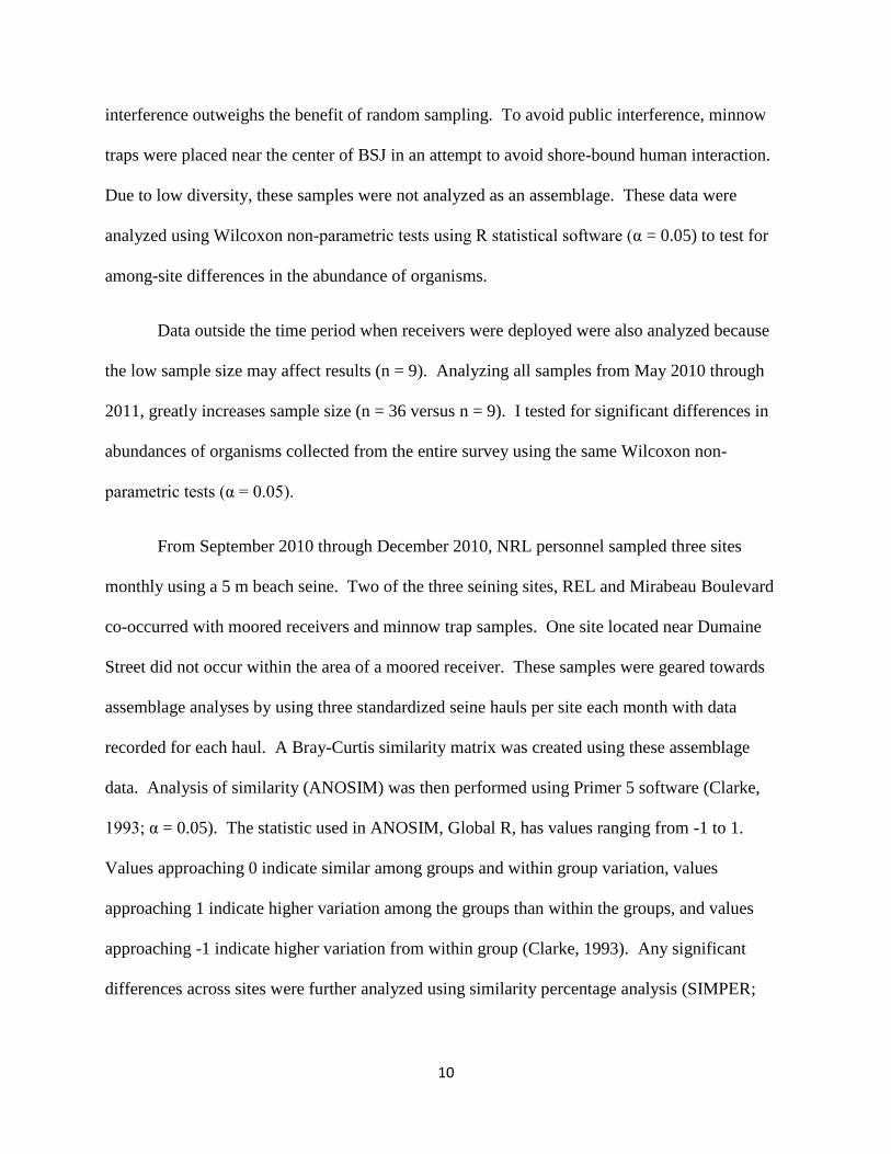
interference outweighs the benefit of random sampling. To avoid public interference, minnow
traps were placed near the center of BSJ in an attempt to avoid shore-bound human interaction.
Due to low diversity, these samples were not analyzed as an assemblage. These data were
analyzed using Wilcoxon non-parametric tests using R statistical software (α = 0.05) to test for
among-site differences in the abundance of organisms.
Data outside the time period when receivers were deployed were also analyzed because
the low sample size may affect results (n = 9). Analyzing all samples from May 2010 through
2011, greatly increases sample size (n = 36 versus n = 9). I tested for significant differences in
abundances of organisms collected from the entire survey using the same Wilcoxon non-
parametric tests (α = 0.05).
From September 2010 through December 2010, NRL personnel sampled three sites
monthly using a 5 m beach seine. Two of the three seining sites, REL and Mirabeau Boulevard
co-occurred with moored receivers and minnow trap samples. One site located near Dumaine
Street did not occur within the area of a moored receiver. These samples were geared towards
assemblage analyses by using three standardized seine hauls per site each month with data
recorded for each haul. A Bray-Curtis similarity matrix was created using these assemblage
data. Analysis of similarity (ANOSIM) was then performed using Primer 5 software (Clarke,
1993; α = 0.05). The statistic used in ANOSIM, Global R, has values ranging from -1 to 1.
Values approaching 0 indicate similar among groups and within group variation, values
approaching 1 indicate higher variation among the groups than within the groups, and values
approaching -1 indicate higher variation from within group (Clarke, 1993). Any significant
differences across sites were further analyzed using similarity percentage analysis (SIMPER;

11
Clarke, 1993). This analysis lists species that contribute most to any dissimilarity displayed in
the pairwise ANOSIM tests.
The species that drive any changes in either of the sampling surveys mentioned above
were compared to the ample list of red drum prey items in the literature. If species that drive the
change in assemblages were considered potentially be prey item(s) for red drum, it was
compared, by inspection, to the daily number of pings near the sampling site. Without any data
on the diet of red drum in BSJ, potential prey items were only referenced with other studies.
Water Quality Modeling
I analyzed continuous water quality data in a way to better understand red drum’s
response to change in abiotic conditions. From 1 September through 31 December 2010, a
remote monitoring continuous water quality station collected specific conductivity, dissolved
oxygen as percent and concentration, salinity, and depth every fifteen minutes in BSJ (Fig. 2).
Data are directly linked to a database web server (YSI - Remote Monitoring and Control System,
2010). The calibration of each station was maintained by The Louisiana State University
Agricultural Center and is currently maintained by the Louisiana Department of Wildlife and
Fisheries. Daily averages from 1 September 2010 through 31 December 2010 were calculated
from this station (Fig. 2). These values are not meant to represent the average daily values for
BSJ’s entirety. The change in these daily values is used to estimate the change across the Bayou.
Analysis of these continuous variables was a multi-step process. The first step was to
determine appropriate tests by analyzing each of the predictor variables. Since specific
conductivity and salinity are different expressions of the same measurement, only one of them is
appropriate for analysis. Salinity was chosen because its values are the most common in the
12
literature and have been found to influence red drum behavior (Dresser and Kneib, 2007;
Bacheler et al., 2009). Dissolved oxygen was represented as both a concentration and as a
percentage. Percent dissolved oxygen is a factor of water temperature, so only dissolved oxygen
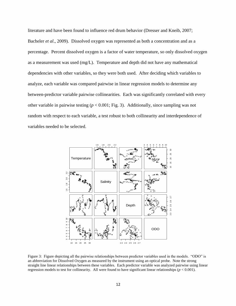
as a measurement was used (mg/L). Temperature and depth did not have any mathematical
dependencies with other variables, so they were both used. After deciding which variables to
analyze, each variable was compared pairwise in linear regression models to determine any
between-predictor variable pairwise collinearities. Each was significantly correlated with every
other variable in pairwise testing (p < 0.001; Fig. 3). Additionally, since sampling was not
random with respect to each variable, a test robust to both collinearity and interdependence of
variables needed to be selected.
Figure 3: Figure depicting all the pairwise relationships between predictor variables used in the models. “ODO” is
an abbreviation for Dissolved Oxygen as measured by the instrument using an optical probe. Note the strong
straight line linear relationships between these variables. Each predictor variable was analyzed pairwise using linear
regression models to test for collinearity. All were found to have significant linear relationships (p < 0.001).
Temperature
1.6 1.8 2.0 2.2 3 4 5 6 7 8 9 10
10
15
20
25
30
1.6
1.8
2.0
2.2
Salinity
Depth
2.3
2.4
2.5
2.6
2.7
10 15 20 25 30
34
56
78
910
2.3 2.4 2.5 2.6 2.7
ODO

13
I chose Generalized Estimating Equations (GEEs) as the most appropriate statistical tool
(Liang and Zeger, 1986). These tests are robust to correlated predictor variables as well as
spatial auto-correlation, and observational correlations. Multiple GEEs, each testing a different
response variable and the same predictor variables, were analyzed. The four response variables
were the number of pings per day from REL, NEI, I610 and the total number of pings per day for
all sites (Total). The predictor variables were salinity, dissolved oxygen concentration, depth,
and temperature. Step-wise model reductions with an exchangeable correlation structure were
performed using the GEEpack for R statistical software (Hojsgaard et al., 2005). Interactions
were not included in these models because all variables were highly correlated.
After determining appropriate analyses and predictor variables, two different approaches
of selecting predictor variable and response variable relationships were used. The first
mentioned here was mathematically driven, and is referred to as “Mathematical Models” or
“Mathematical GEEs”. These used multiple regressions to determine the relationship between
each predictor variable – response variable relationship. This approach was unbiased in that
logical or practical relationships between variables were not considered. The second approach I
considered was driven by logical and practical relationships, and is referred to as “Practical
Models” or “Practical GEEs”. These models were based relationships that seemed likely to
occur in nature. Once the relationship between each variable was established using each
approach, a GEE step-wise model reduction comparing each response variable (REL, NEI, I610,
Total) against all four predictor variables (salinity, dissolved oxygen concentration, depth, and
temperature) was developed.

14
Mathematical Models
Before analyzing all of the variables in one model, the relationship between each
predictor and explanatory variable was determined. In order to do this, I fitted several regression
models between each predictor variable and explanatory variable in a stepwise manner. First,
linear models were tested and then higher order polynomials were added until the addition of one
did not significantly increase the amount of variation explained by the predictor variable for the
response variable (α = 0.05). The highest order polynomial fit that significantly increased the
amount of variance explained in the regression model was chosen to represent the relationship
between predictor and explanatory variable.
Practical Models
Each of the variables used in the Practical GEEs were based on what makes the most
ecological sense. Between mean daily temperature and the number of pings per day, a second-
order relationship seems likely, suggesting that data including temperatures below, above, and
optimal for red drum activity. It is likely that this occurred in our study period at our site based
upon a review of red drum’s natural range (Massachusetts to Northern Mexico; Matlock, 1987)
and aquaculture experiments (Thomas, 1991). Salinity has been shown to influence red drum
habitat selection, with either low or high values being selected (Bacheler, 2009). Therefore, a
straight line linear relationship between salinity and the mean number of pings per day was
chosen. Similarly, depth has been shown to be a good predictor of red drum habitat selections,
with different habitats being selected at low and high values (Dresser and Kneib, 2007). Like
salinity, a straight line linear relationship was chosen for depth. Dissolved oxygen was not
considered in any of these models. This was because the most logical response to dissolved
15
oxygen would be avoidance of an area based on low dissolved oxygen levels. Since there was
only one station where dissolved oxygen was recorded, it was not included in the Practical
Models. Additionally, an aquaculture study found juvenile red drum to be tolerant of low
dissolved concentrations (< 3.0 mg/L; Thomas, 1991).
Results
Prey Abundances
The number of pings detected at each site was found to be significantly different
(ANOVA, F = 186.1, p < 0.001). Tukey’s post hoc analysis was performed and found that each
pairwise test between sites was significantly different (REL~NEI: p < 0.001; REL~I610: p <
0.001; NEI~I610: p < 0.001). Higher mean daily pings were found for REL followed by NEI,
I610 had the lowest mean daily pings (REL = 273.6311, s.d. = 173.3973; NEI = 94.6056, s.d. =
86.84569; I.610 = 1.42623, s.d. = 5.52368; Fig. 4).

16
Figure 4: Box plot of mean, mode, and standard deviation in the number of pings per day for each site from
September through December 2010, where I610 is Interstate 610, NEI is North End Island, and REL is Robert E.
Lee. A ping occurs whenever a tagged red drum is within a receiver located at any of the three sites. The y-axis is
the number of pings per day and the x-axis is the factor site.
For the entire study (May 2010 – May 2011), four species, estuarine mud crab
(Rhithropanopeus harrisii; Family: Xanthidae), bluegill (Lepomis macrochirus), M. salmoides,
and Gulf pipefish (Syngnathus scovelli) were collected as a part of the benthic epifaunal minnow
trap survey (Table 1). Of these four species, only abundances of R. harrisii were analyzed using
Wilcoxon non parametric tests. No analyses were conducted on the other species because of
their low abundances.

17
During the study period of September through December 2010, two species were
sampled, R. harrisii and L. macrochirus (Table 2). Again, only R. harrisii abundances were
analyzed due to low abundances of L. macrochirus. Pairwise tests between Robert E. Lee and
both of the other sites were found to be significantly different (Wilcoxon; REL vs. NEI: W =
62.5, p = 0.03585; REL vs. I610: W = 65, p = 0.01558). The pairwise test between North End
Island and Interstate 610 was not found to be significant (Wilcoxon, W = 36, p = 0.5848; Table
5). The average number of mud crabs sampled was found to be higher for REL than NEI or I610
(REL: μ= 1.889 s.d. = 1.900; NEI: μ= 0.222, s.d. = 0.441; I610: μ= 0.333 s.d. = 0.333; Fig. 5).
Table 1. Number of individuals for each species collected from minnow traps sampled in Bayou St. John from May
2010 through May 2011 per site and overall. Triplicate samples were collected monthly as per the methods, except
for the month of November (n=108).
Species and Number Collected per Site (5/1/2010 – 5/31/2011)
Site
Rhithropanopeus
harrisii
(estuarine mud
crab)
Lepomis
macrochirus
(bluegill)
Micropterus
salmoides
(largemouth
bass)
Syngnathus
scovelli
(Gulf pipefish)
REL 29 4 0 2
NEI 23 1 2 0
I610 33 10 0 0
Total 85 15 2 2
Table 2. Number of individuals for each species collected from minnow traps sampled in Bayou St. John from
September through December 2010 per site and overall. Triplicate samples were collected monthly as per the
methods, except for the month of November (n=27).
Species and Number Collected per Site (9/1/2010 – 12/31/2010)
Site
Rhithropanopeus
harrisii
(estuarine mud
crab)
Lepomis
macrochirus
(bluegill)
Micropterus
salmoides
(largemouth
bass)
Syngnathus
scovelli
(Gulf pipefish)
REL 21 1 0 0
NEI 3 0 0 0
I610 4 7 0 0
Total 28 8 0 0

18
Figure 5: Box plot of mean, mode, and standard deviation in the number of R. harrisii collected per replicate for
each site from September through December 2010, where I610 is Interstate 610, NEI is North End Island, and REL
is Robert E. Lee. The mean and standard deviation for each site was REL: μ= 1.889 s.d. = 1.900; NEI: μ= 0.222,
s.d. = 0.441; I610: μ= 0.333 s.d. = 0.333. The y-axis represents the number of R. harrisii per replicate and the x-axis
is the factor site.
The results from the entire study period (May 2010 – May 2011) suggest that there is no
significant difference among sites as a result of pairwise Wilcoxon tests (REL ~ NEI: W = 597.5,
p = 0.5206, REL ~ I610: W = 670, p = 0.7882, NEI~I610: W = 718, p = 0.3744). Also, the mean
and standard deviation for REL, NEI, and I610 were similar and all less than one, μ= 0.806, s.d.
= 1.261; μ= 0.639, s.d. = 1.099; μ= 0.9167 s.d. = 1.380, respectively (Fig. 6). These results
suggest similarly low R. harrisii numbers among all sites.

19
Figure 6: Box plot of mean, mode, and standard deviation in the number of R. harrisii collected per replicate for
each site from May 2010 through May 2011, where I610 is Interstate 610, NEI is North End Island, and REL is
Robert E. Lee. The mean and standard deviation for each site was REL: μ = 0.806 s.d. = 1.261; NEI: μ = 0.639, s.d.
= 1.099; I610: μ = 0.9167 s.d. = 1.380. The y-axis represents the number of R. harrisii per replicate and the x-axis is
the factor site.
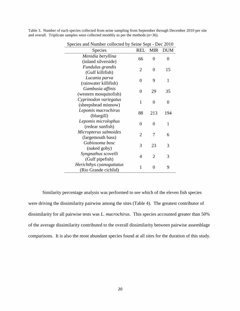
Eleven species of fishes were sampled from September through December 2010 as a part
of a shoreline seining survey (Table 3) and a significant difference in assemblage composition
was exhibited among sites (ANOSIM, Global R = 0.266, p = 0.001). Pairwise tests between the
sites indicated that each site was significantly different from every other site (REL vs. MIR, R =
0.493, p = 0.001; REL vs. DUM, R = 0.142, p = 0.02; DUM vs. MIR, R = 0.179, p = 0.014).
20
Table 3. Number of each species collected from seine sampling from September through December 2010 per site
and overall. Triplicate samples were collected monthly as per the methods (n=36).
Species and Number collected by Seine Sept - Dec 2010
Species REL MIR DUM
Menidia beryllina
(inland silverside) 66 0 0
Fundulus grandis
(Gulf killifish) 2 0 15
Lucania parva
(rainwater killifish) 0 9 1
Gambusia affinis
(western mosquitofish) 0 29 35
Cyprinodon variegatus
(sheepshead minnow) 1 0 0
Lepomis macrochirus
(bluegill) 88 213 194
Lepomis microlophus
(redear sunfish) 0 0 1
Micropterus salmoides
(largemouth bass) 2 7 6
Gobiosoma bosc
(naked goby) 3 23 3
Syngnathus scovelli
(Gulf pipefish) 4 2 3
Herichthys cyanoguttatus
(Rio Grande cichlid) 1 0 9
Similarity percentage analysis was performed to see which of the eleven fish species
were driving the dissimilarity pairwise among the sites (Table 4). The greatest contributor of
dissimilarity for all pairwise tests was L. macrochirus. This species accounted greater than 50%
of the average dissimilarity contributed to the overall dissimilarity between pairwise assemblage
comparisons. It is also the most abundant species found at all sites for the duration of this study.

21
Table 4. Similarity Percentages (SIMPER) results for fish assemblages collected in the shoreline habitat from
September through December 2010. Only the species that contributed up to 90% of the total assemblage change are
shown. Values in the Contribution percentage column represent the average dissimilarity each species contributed
to the overall dissimilarity between assemblages.
SIMPER Analysis Results
Robert E. Lee and Mirabeau
Species REL Mean
Abundance
Mirabeau Mean
Abundance
Mean
Dissimilarity
Contribution
%
Lepomis macrochirus 7.33 17.75 49.35 59.66
Menidia beryllina 5.5 0 12.77 15.43
Gambusia affinis 0 2.42 7.23 8.74
Gobiosoma bosc 0.25 1.92 5.39 6.51
Robert E. Lee and Dumaine
Species REL Mean
Abundance
Dumaine Mean
Abundance
Mean
Dissimilarity
Contribution
%
Lepomis macrochirus 7.33 16.17 36.77 62.58
Menidia beryllina 5.5 0 17.13 14.87
Gambusia affinis 0 2.92 8.81 7.44
Micropterus salmoides 0.17 0.5 4.35 4.3
Herichthys cyanoguttatus 0.08 0.75 3.61 3.99
Mirabeau and Dumaine
Species Mirabeau Mean
Abundance
Dumaine Mean
Abundance
Mean
Dissimilarity
Contribution
%
Lepomis macrochirus 17.75 16.17 39.67 62.58
Gambusia affinis 2.42 2.92 9.42 14.87
Gobiosoma bosc 1.92 0.25 4.72 7.44
Lucania parva 0.75 0.08 2.79 4.3
Micropterus salmoides 0.58 0.52 2.53 3.99
Water Quality Modeling
Mean daily values for all abiotic data (based on measurements every 15 minutes) were
calculated and plotted against time measured in days (Figs. 7, 8, 9, and 10). High daily mean
temperature was on 12 September 2010 at 31.91°C and low daily mean temperature was on 27
December 2010 at 8.73°C (Fig. 7). Overall, daily mean temperature declined over the study

22
period (Fig. 7). High daily mean salinity was on 31 December 2010 at 2.24, and low daily mean
salinity was on 2 September 2010 at 1.54 (Fig. 8). Daily mean salinity increased over the study
period (Fig. 8). High daily mean depth was on 3 November 2010 at 2.74 m, and low daily mean
depth was on 12 October 2010 at 2.28 m (Fig. 9). There was no marked overall trend in mean
depth over time (Fig. 9). High daily mean dissolved oxygen was on 14 December 2010 at 10.05
mg/L and low daily mean dissolved oxygen was on 25 October 2010 at 3.25 mg/L (Fig. 10).
Mean daily dissolved oxygen appeared to increase over the study period (Fig, 10).
Figure 7: Daily mean temperature (°C) over the study period (1 September through 31 December 2011). Each point
represents a calculated mean, with a line connecting the points to show the overall trend.
0
5
10
15
20
25
30
35
September-10 October-10 November-10 December-10 January-11
Tem
per
atu
re (°C
)
Month
Daily Mean Temperature

23
Figure 8: Daily mean salinity over the study period (1 September through 31 December 2011). Each point
represents a calculated mean, with a line connecting the points to show the overall trend.
1.5
1.6
1.7
1.8
1.9
2
2.1
2.2
2.3
September-10 October-10 November-10 December-10 January-11
Sali
nit
y
Month
Daily Mean Salinity

24
Figure 9: Daily mean depth (m) over the study period (1 September through 31 December 2011). Each point
represents a calculated mean, with a line connecting the points to show the overall trend.
2
2.1
2.2
2.3
2.4
2.5
2.6
2.7
2.8
September-10 October-10 November-10 December-10 January-11
Dep
th (
m)
Month
Daily Mean Depth

25
Figure 10: Daily mean dissolved oxygen (mg/L) over the study period (1 September through 31 December 2011).
Each point represents a calculated mean, with a line connecting the points to show the overall trend.
Mathematical Models
The order of the relationship between each predictor variable and all four response
variables was determined by a multistep process. Each ordinal relationship had to pass two tests.
First, the predictor variable had to explain a statistically significant amount of variation in the
response variable, and second, it had to explain significantly more variation in the response
variable than other exponential values of predictor variables. For the number of pings per day at
REL, a quadratic relationship was chosen for temperature and salinity (p = 0.0001, p = 3.47x10-
10; respectively; Table 5, Figs. 11 and 12), a straight line linear relationship was chosen for
dissolved oxygen (p = 0.01204; Table 5, Fig. 13), and no relationship could be determined with
respect to depth (p = 0.085, quadratic; Table 5, Fig. 14). For the number of pings per day at NEI,
0
2
4
6
8
10
12
September-10 October-10 November-10 December-10 January-11
Dis
solv
ed O
xygen
(m
g/L
)
Month
Daily Mean Dissolved Oxygen

26
a quadratic relationship was chosen for temperature and dissolved oxygen (p = 1.99x10⁻¹³
, p =
0.00163; respectively; Table 6, Figs. 15 and 17), a cubic relationship fit best for salinity (p =
1.14x10⁻⁸
; Table 6, Fig. 16), and no relationship could be determined with respect to depth (p =
0.198, linear; Table 6, Fig. 12). No significant relationships between any abiotic variable and the
number of pings per day at I610 could be determined (Table 7). For the total number of pings
per day, a quadratic relationship was chosen for temperature and dissolved oxygen (p = 2.98x10-
10, p = 0.0123; respectively; Table 8, Figs. 18 and 20), a cubic relationship was chosen for
salinity (p = 0.00914; Table 8, Fig. 119), and no relationship could be determined with respect to
depth (p = 0.0635, quadratic; Table 8).
Table 5. Results from multiple regressions models comparing the number of pings per day at Site Robert E. Lee
versus all four predictor variables (Temperature, Salinity, Dissolved Oxygen, and Depth). Rows labeled “GLT”
indicate the p-value associated between two models, one with the variable noted, one included only the next lowest
variable by the general linear test. Each section highlighted in gray represents the best fitting relationship for each
variable.
REL Polynomial Test Results
WQ Variable Linear Quad Cubic
Temp
p-value 0.0282 5.60E-05 1.49E-04
R2 0.03149 0.1375 0.1359
GLT 1.27E-04 0.3789226
Salinity
p-value 0.01204 1.03E-10 4.59E-10
R2 0.04349 0.3091 0.307
GLT 3.47E-10 4.24E-01
DO
p-value 0.00261 4.16E-03 1.12E-02
R2 0.06532 0.07269 0.06623
GLT 0.1662 0.6754
Depth
p-value 0.6237 0.08532 0.1535
R2 -0.006304 0.0244 0.01912
GLT 0.03127 0.54966

27
Table 6. Results from multiple regressions modeling comparing the number of pings per day at Site North End
Island versus all four predictor variables (Temperature, Salinity, Dissolved Oxygen, and Depth). Rows labeled
“GLT” indicate the p-value associated between two models, one with the variable noted, one included only the next
lowest variable by the general linear test. Each section highlighted in gray represents the best fitting relationship for
each variable.
NEI Polynomial Test Results
WQ Variable Linear Quad Cubic
Temp
p-value 0.327 9.06E-13 4.80E-12
R2 -0.0002597 0.362 0.3593
GLT 1.99E-13 0.4762
Salinity
p-value 0.1062 7.70E-09 4.15E-15
R2 0.01345 0.2572 0.4323
GLT 4.28E-11 1.14E-08
DO
p-value 0.09098 1.58E-03 4.95E-03
r^2 0.01549 0.08765 0.08005
GLT 0.001627 0.894456
Depth
p-value 0.1978 0.2843 0.4654
R2 0.005563 0.004463 -0.003551
GLT 0.3555 0.8241
Table 7. Results from multiple regressions modeling comparing the number of pings per day at Site I610 versus all
four predictor variables (Temperature, Salinity, Dissolved Oxygen, and Depth). Rows labeled “GLT” indicate the p-
value associated between two models, one with the variable noted, one included only the next lowest variable by the
general linear test. Each section highlighted in gray represents the best fitting relationship for each variable.
I-610 Polynomial Test Results
WQ Variable Linear Quad Cubic
Temp
p-value 0.9955 1.57E-01 1.79E-01
R2 -0.008333 0.01434 0.01615
GLT 5.47E-02 0.2718
Salinity
p-value 0.7324 1.24E-01 0.1288
R2 -0.007347 0.0182 0.02249
GLT 4.41E-02 0.21971
DO
p-value 0.7886 8.76E-01 6.13E-01
R2 -0.007727 -0.01455 -0.009887
GLT 0.6605 0.2157
Depth
p-value 0.4254 0.3602 0.5536
R2 -0.002986 0.0004958 -0.007483
GLT 0.238 0.8109
28
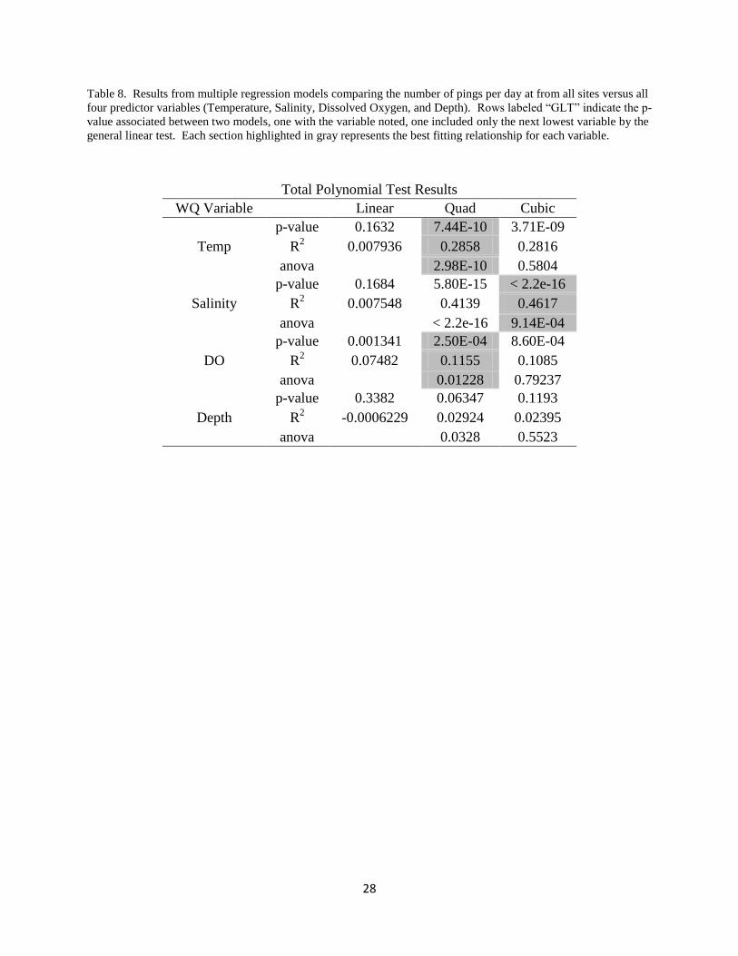
Table 8. Results from multiple regression models comparing the number of pings per day at from all sites versus all
four predictor variables (Temperature, Salinity, Dissolved Oxygen, and Depth). Rows labeled “GLT” indicate the p-
value associated between two models, one with the variable noted, one included only the next lowest variable by the
general linear test. Each section highlighted in gray represents the best fitting relationship for each variable.
Total Polynomial Test Results
WQ Variable Linear Quad Cubic
Temp
p-value 0.1632 7.44E-10 3.71E-09
R2 0.007936 0.2858 0.2816
anova 2.98E-10 0.5804
Salinity
p-value 0.1684 5.80E-15 < 2.2e-16
R2 0.007548 0.4139 0.4617
anova < 2.2e-16 9.14E-04
DO
p-value 0.001341 2.50E-04 8.60E-04
R2 0.07482 0.1155 0.1085
anova 0.01228 0.79237
Depth
p-value 0.3382 0.06347 0.1193
R2 -0.0006229 0.02924 0.02395
anova 0.0328 0.5523

29
Figure 11: Relationship between the number of pings per day at Site Robert E. Lee (y-axis) and the daily mean
temperature value in °C (x-axis) as a scatter plot with line of best fit. The line of best fit generated from multiple
regression models indicates a quadratic relationship (p = 5.06x10⁻⁵
).
0
100
200
300
400
500
600
700
800
5 10 15 20 25 30 35
Nu
mb
er o
f P
ing
s p
er D
ay
Temperature (°C)
REL Pings vs. Temperature
30
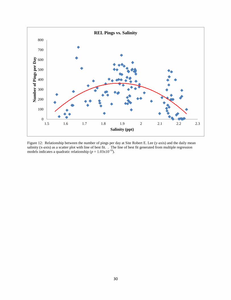
Figure 12: Relationship between the number of pings per day at Site Robert E. Lee (y-axis) and the daily mean
salinity (x-axis) as a scatter plot with line of best fit. . The line of best fit generated from multiple regression
models indicates a quadratic relationship (p = 1.03x10⁻¹⁰
).
0
100
200
300
400
500
600
700
800
1.5 1.6 1.7 1.8 1.9 2 2.1 2.2 2.3
Nu
mb
er o
f P
ing
s p
er D
ay
Salinity (ppt)
REL Pings vs. Salinity

31
Figure 13: Relationship between the number of pings per day at Site Robert E. Lee (y-axis) and the daily mean
dissolved oxygen value (mg/L; x-axis) as a scatter plot with line of best fit. The line of best fit generated from
multiple regression models indicates a linear relationship (p = 0.00261).
0
100
200
300
400
500
600
700
800
2 3 4 5 6 7 8 9 10 11
Nu
mb
er o
f P
ing
s p
er D
ay
Dissolved Oxygen (mg/L)
REL Pings vs. Dissolved Oxygen

32
Figure 14: Relationship between the number of pings per day at North End Island (y-axis) and the daily mean
temperature value (°C; x-axis) as a scatter plot with line of best fit. The line of best fit generated from multiple
regression models indicates a quadratic relationship (p = 9.06x10⁻¹³
).
0
50
100
150
200
250
300
350
400
5 10 15 20 25 30 35
Nu
mb
er o
f P
ing
s p
er D
ay
Temperature (°C)
NEI Pings vs. Temperature
33
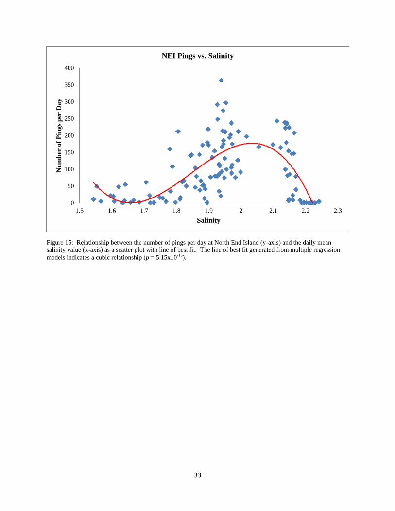
Figure 15: Relationship between the number of pings per day at North End Island (y-axis) and the daily mean
salinity value (x-axis) as a scatter plot with line of best fit. The line of best fit generated from multiple regression
models indicates a cubic relationship (p = 5.15x10⁻¹⁵
).
0
50
100
150
200
250
300
350
400
1.5 1.6 1.7 1.8 1.9 2 2.1 2.2 2.3
Nu
mb
er o
f P
ing
s p
er D
ay
Salinity
NEI Pings vs. Salinity

34
Figure 16: Relationship between the number of pings per day at North End Island (y-axis) and the daily mean
dissolved oxygen value (mg/L; x-axis) as a scatter plot with line of best fit. The line of best fit generated from
multiple regression models indicates a quadratic relationship (p = 0.00158).
0
50
100
150
200
250
300
350
400
2 3 4 5 6 7 8 9 10 11
Nu
mb
er o
f P
ing
s p
er D
ay
Dissolved Oxygen (mg/L)
NEI Pings vs. Dissolved Oxygen

35
Figure 17: Relationship between the total number of pings per day (y-axis) and the daily mean temperature value
(°C; x-axis) as a scatter plot with line of best fit. The line of best fit generated from multiple regression models
indicates a quadratic relationship (p = 7.44x10⁻¹⁰
).
0
100
200
300
400
500
600
700
800
900
5 10 15 20 25 30 35
Nu
mb
er o
f P
ing
s p
er D
ay
Temperature (°C)
Total Pings vs. Temperature

36
Figure 18: Relationship between the total number of pings per day (y-axis) and the daily mean salinity value (x-
axis) as a scatter plot with line of best fit. The line of best fit generated from multiple regression models indicates a
cubic relationship (p < 2.2x10⁻¹⁶
).
0
100
200
300
400
500
600
700
800
900
1.3 1.5 1.7 1.9 2.1 2.3 2.5
Nu
mb
er o
f P
ing
s p
er D
ay
Daily Mean Salinity
Total Pings vs. Salinity

37
Figure 19: Relationship between the total number of pings per day (y-axis) and the daily mean dissolved oxygen
value (mg/L; x-axis) as a scatter plot with line of best fit. The line of best fit generated from multiple regression
models indicates a cubic relationship (p = 0.00025).
Mathematical GEE predictor variables were selected based on the above analysis. That
is, the polynomial order for each predictor variable response variable pairing was selected based
upon the above criteria. Then, three GEEs step-wise model reductions were performed. Similar
to the multiple regression analyses above, no model reduction for I610 could be done because
these data were unable to be transformed to fit any distributional pattern. This may have been
due to low number of pings throughout the study, 95 of 122 days (78%) during this study 0 pings
were detected at I610 (Fig. 20).
0
100
200
300
400
500
600
700
800
900
2 3 4 5 6 7 8 9 10 11
Nu
mb
er o
f P
ing
s p
er D
ay
Dissolved Oxygen (mg/L)
Total Pings vs. Dissolved Oxygen

38
Figure 20: Frequency histogram depicting the number of pings detected per day as a percent total. This distribution
shows a high frequency of low numbers, with 78% of all days having 0 detections.
REL’s Mathematical GEE correlation structure was exchangeable, also termed compound
symmetry correlation structure, and Gaussian distribution of errors. Before reduction, the model
was y = β1T + β2T2 + β3S + β4S
2 + β5D + β0 + ε, where y = number of pings per day at Robert E.
Lee, T = daily mean temperature value, S = daily mean salinity value, and D = daily mean
dissolved oxygen value. Variables were reduced stepwise, with higher order polynomials of
each predictor being reduced first. The resulting model was reduced to y = β1T + β2S + β3S2 + β0
+ ε. (W = 4.5, p = 0.0000054; Table 9). The result included temperature as a first order
polynomial and salinity as a second order polynomial as significant predictor variables.

39
Table 9. Table showing the results of a generalized estimating equation (GEE) step-wise model reduction of the
original model that included: y = β1T + β2T2 + β3S + β4S
2 + β5D + β0 + ε, where y = number of pings per day at
Robert E. Lee, T = daily mean temperature value, S = daily mean salinity value, and D = daily mean dissolved
oxygen value. The model was reduced to y = β1T + β2S + β3S2 + β0 + ε.
GEE stepwise reduction model REL
Distribution = Gaussian, Correlation = compound symmetry
Estimate Standard Error Wald Statistic p-value
Intercept -8647.9 1235.5 49 2.60E-12
Temperature -20.5 4.5 20.7 5.40E-06
Salinity 10760.9 1307.2 67.8 2.20E-16
Salinity2 -3030 345.4 77 < 2E-16
The Mathematical GEE for NEI correlation structure was exchangeable and Gaussian
distribution of errors. Before reduction, the model was y = β1T + β2T2 + β3S + β4S
2 + β5S
3 + β6D
+ β7D2 + β0 + ε, where y = number of pings per day at North End Island, T = daily mean
temperature value, S = daily mean salinity value, and D = daily mean dissolved oxygen value.
Variables were reduced stepwise, with higher order polynomials of each predictor being reduced
first. The resulting model was reduced to y = β1S + β2S2 + β3S
3+ β0 + ε. (W statistic = 34.2, p <
2x10-16
, Table 10). Results included salinity as a third order polynomial as the significant
predictor variables.
Table 10. Results of a generalized estimating equation (GEE) step-wise model reduction of the original model that
included: y = β1T + β2T2 + β3S + β4S
2 + β5S
3 + β6D + β7D
2 + β0 + ε, where y = number of pings per day at North
End Island, T = daily mean temperature value, S = daily mean salinity value, and D = daily mean dissolved oxygen
value. The model was reduced to y = β1S + β2S2 + β3S
3+ β0 + ε.
GEE stepwise reduction model NEI
Distribution = Poisson, Correlation = compound symmetry
Estimate Standard Error Wald Statistic p-value
Intercept 541.2 102 28.2 2.60E-12
Salinity -895 163.4 30 5.40E-06
Salinity2 491.6 86.7 32.2 2.20E-16
Salinity3 -89 15.2 34.2 < 2E-16

40
Total’s (the total number of pings per day, including all sites) Mathematical GEE
correlation structure was exchangeable and Gaussian distribution of errors. Before reduction, the
model was y = β1T + β2T2 + β3S + β4S
2 + β5S
3 + β6D + β7D
2 + β0 + ε, where y = total number of
pings per day, T = daily mean temperature value, S = daily mean salinity value, and D = daily
mean dissolved oxygen value. Variables were reduced stepwise, with higher order polynomials
of each predictor being reduced first. The resulting model was reduced to y = β1T + β2T2 + β3S +
β4S2+ β0 + ε. (W statistic = 5.12, p = 0.024; Table 11). Results included temperature as a second
order polynomial and salinity as a second order polynomial as predictor variables.
Table 11. Results of a generalized estimating equation (GEE) step-wise model reduction of the original model that
included: y = β1T + β2T2 + β3S + β4S
2 + β5S
3 + β6D + β7D
2 + β0 + ε, where y = the total number of pings per day for
all sites, T = daily mean temperature value, S = daily mean salinity value, and D = daily mean dissolved oxygen
value. The model was reduced to y = β1T + β2T2 + β3S + β4S
2 + β0 + ε.
GEE stepwise reduction model Total
Distribution = Gaussian, Correlation = compound symmetry
Estimate Standard Error Wald Statistic p-value
Intercept -10900 1400 60.68 6.70E-15
Temperature 11.9 16.6 0.52 4.72E-01
Temperature2 -0.838 -0.37 5.12 2.40E-02
Salinity 13000 1600 66.13 4.4E-16
Salinity2 -3620 43 70.8 < 2E-16
Practical Models
REL’s Practical GEE was exchangeable and Gaussian distribution of errors. Before
reduction, the model was y = β1T + β2T2 + β3S + β4D + β0 + ε, where y = number of pings per
day at REL, T = daily mean temperature value, S = daily mean salinity value, and D = daily
mean depth value. Variables were reduced stepwise, with higher order polynomials of each
predictor being reduced first. The resulting model was reduced to y = β1T + β2T2+ β3S + β0 + ε.
(W = 5.24, p = 0.02212; Table 12). The result included temperature as a second order

41
polynomial and salinity as a first order polynomial as significant predictor variables. The
straight line relationship between salinity and the number of pings per day at REL is a negative
correlation (Fig. 21).
Figure 21: Graph showing the relationship between the number of pings per day at the Robert E. Lee site (y-axis)
and the daily mean salinity value (x-axis) as a scatter plot. The fitted line (in red) shows the first-order polynomial
line of best fit generated from a regression model.
0
100
200
300
400
500
600
700
800
1.5 1.6 1.7 1.8 1.9 2 2.1 2.2 2.3
Nu
mb
er o
f P
ings
per
Da
y
Salinity (ppt)
REL Pings vs. Salinity
42
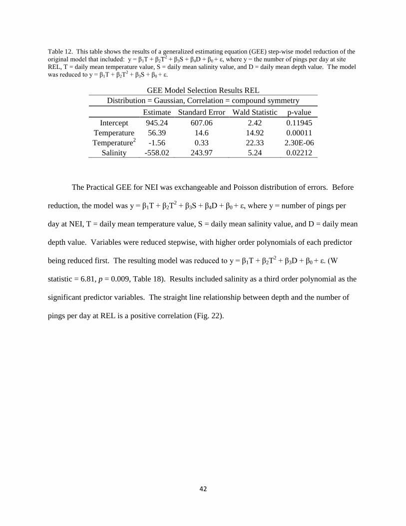
Table 12. This table shows the results of a generalized estimating equation (GEE) step-wise model reduction of the
original model that included: y = β1T + β2T2 + β3S + β4D + β0 + ε, where y = the number of pings per day at site
REL, T = daily mean temperature value, S = daily mean salinity value, and D = daily mean depth value. The model
was reduced to y = β1T + β2T2 + β3S + β0 + ε.
GEE Model Selection Results REL
Distribution = Gaussian, Correlation = compound symmetry
Estimate Standard Error Wald Statistic p-value
Intercept 945.24 607.06 2.42 0.11945
Temperature 56.39 14.6 14.92 0.00011
Temperature2 -1.56 0.33 22.33 2.30E-06
Salinity -558.02 243.97 5.24 0.02212
The Practical GEE for NEI was exchangeable and Poisson distribution of errors. Before
reduction, the model was y = β1T + β2T2 + β3S + β4D + β0 + ε, where y = number of pings per
day at NEI, T = daily mean temperature value, S = daily mean salinity value, and D = daily mean
depth value. Variables were reduced stepwise, with higher order polynomials of each predictor
being reduced first. The resulting model was reduced to y = β1T + β2T2 + β3D + β0 + ε. (W
statistic = 6.81, p = 0.009, Table 18). Results included salinity as a third order polynomial as the
significant predictor variables. The straight line relationship between depth and the number of
pings per day at REL is a positive correlation (Fig. 22).

43
Figure 22: Graph showing the relationship between the number of pings per day at North End Island site (y-axis)
and the daily mean depth in meters (x-axis) as a scatter plot. The fitted line (in red) shows the first-order polynomial
line of best fit generated from a regression model.
Table 13. Results of a generalized estimating equation (GEE) step-wise model reduction of the original model that
included: y = β1T + β2T2 + β3S + β4D + β0 + ε, where y = the number of pings per day at site NEI, T = daily mean
temperature value, S = daily mean salinity value and D = daily mean depth value. The model was reduced to y =
β1T + β2T2 + β3D + β0 + ε.
GEE Model Selection Results NEI
Distribution = Poisson, Correlation = compound symmetry
Estimate Standard Error Wald Statistic p-value
Intercept -4.58497 1.61866 8.02 0.0046
Temperature 0.65758 0.10633 38.24 6.20E-10
Temperature2 -0.01631 0.00241 45.82 2.30E-06
Depth 1.22792 0.47041 6.81 0.009
Total’s (the total number of pings per day, including all sites) Practical GEE was
exchangeable and Gaussian distribution of errors. Before reduction, the model was y = β1T +
β2T2 + β3S + β4D + β0 + ε, where y = total number of pings per day, T = daily mean temperature
0
50
100
150
200
250
300
350
400
2.2 2.3 2.4 2.5 2.6 2.7 2.8
Nu
mb
er o
f P
ing
s p
er D
ay
Depth (m)
NEI Pings vs. Depth

44
value, S = daily mean salinity value, and D = daily mean depth value. Variables were reduced
stepwise, with higher order polynomials of each variable being reduced first. The resulting
model was reduced to y = β1T + β2T2 + β0 + ε. (W statistic = 47, p = 7.10x10
-12; Table 14).
Results included temperature as a second order polynomial as predictor variables.
Table 14. Results of a generalized estimating equation (GEE) step-wise model reduction of the original model that
included: y = β1T + β2T2 + β3S + β4D + β0 + ε, where y = the total number of pings per day from all sites, T = daily
mean temperature value, S = daily mean salinity value, and D = daily mean depth value. The model was reduced to
y = β1T + β2T2 + β0 + ε.
GEE Model Selection Results Total
Distribution = Gaussian, Correlation = compound symmetry
Estimate Standard Error Wald Statistic p-value
Intercept -704.133 152.342 21.4 3.80E-06
Temperature 110.585 0.10633 50.8 1.00E-12
Temperature2 -2.559 0.373 47 7.10E-12
Discussion
Prey Availability and Red Drum Location
My results on the number of pings per day (indicating the presence of a tagged red drum)
support the previous findings with the highest number of pings occurring in the northernmost site
(Brogan, 2010). The average number of pings for the most southern site (I610) was markedly
low (1.43 + 5.52), which also agrees with the previous study (Brogan, 2010). The results from
both studies suggest that red drum are avoiding areas south of I610.
The possibility that red drum can pass a receiver without detection is low. The maximum
overall width of BSJ is 200 m. Based upon expected detection radius for the receivers, tagged
red drum cannot swim throughout the Bayou without passing within the range of detection for
the receiver transmitter combination (between 300-540 m, depending on conditions). The

45
transmitters were designed to send a ping every 180 seconds on average (Brogan, 2010). With
this interval, a tagged fish could potentially pass through a receiver’s range of detection without
the transmitter sending a signal. However, there were no instances where a red drum was
detected at REL and then detected at I610, or vice versa. Additionally, the middle receiver (NEI)
is near the widest point in the Bayou. This suggests that a red drum cannot easily travel through
a receiver’s detection radius without being recorded.
Of the twelve organisms sampled in both the shoreline and the epibenthic surveys, five
have been observed as stomach contents for large (> 300 mm) juvenile red drum in the literature:
Menidia beryllina (inland silverside), Cyprinodon variegatus (sheepshead minnow), Gobiosoma
bosc (naked goby), Fundulus grandis (Gulf killifish), and R. harrisii (Boothby and Avault Jr.,
1971; Overstreet and Heard, 1978). Across studies, red drum were found to ingest abundant crab
species, with Xanthid crabs being particularly important in impoundments (Llanso et al., 1998;
Matlock, 1987). Teleost fishes were not found to be as important a food item as crabs (Boothby
and Avault Jr., 1971; Overstreet and Heard, 1978; Llanso et la., 1998). The only stomach
content observed in a red drum from BSJ was a C. sapidus (Brogan, 2010). Additionally, most
research suggests blue crabs are the primary prey item for red drum (Guillory and Prejean,
1999). No blue crabs were ever sampled at any of the sites during this period. Without more
knowledge of the actual diet of BSJ red drum, it is difficult to determine which prey items this
species prefers.
If the abundance of potential prey items are an important reason why the southern portion
of BSJ is underutilized, differences in prey items would have been observed across broad
temporal periods because red drum have been found in the northern sites in BSJ across all
methods and studies. On average, more organisms were observed at the northernmost site than

46
the other sites from September through December 2010. At first glance, this may lead to the
conclusion that higher abundances occur at the same site in which higher numbers of pings per
day do. However, the standard deviation for each site is greater than or equal to the mean for
each site, suggesting that means are still low overall and the dataset is zero-inflated.
Additionally, when analyzing a much larger dataset (May 2010 – May 2011), no statistically
significant difference was observed for any pairwise combination. Since previous studies show a
similar relationship for the total number of pings per site and the larger dataset does not reveal a
statistically significant difference among sites, the correlation between the number of pings per
site and higher abundances of R. harrisii seen during September through December 2010 may be
a statistical artifact that does not reflect actual relationships. Possibly, the apparent relationship
may be due to low sample size (n = 27). Selection of habitat based up prey items could not be
inferred using data from the benthic survey.
One of the issues concerning analysis of the shoreline assemblages is the lack of overlap
between receiver site I610 and seining site at Dumaine Bridge. The number of pings per day at
I610 was low, with the vast majority of the days having zero pings recorded. This ultimately is
more problematic than the lack of overlap between sampling sites, because of a heavily zero-
weighted dataset. Therefore, the only conclusion that can come from analysis of pings per day at
I610 is they are low to the point of almost complete avoidance. Therefore any assemblage
difference at Dumaine Bridge could be considered a surrogate for habitats with extremely low
red drum occurrences.
Lower abundances of all organisms, except one, that contributed to assemblage
differences between pairwise site tests were observed at REL. Only M. beryllina was observed
in higher abundances at REL and it was not collected at the other sites. However, these fishes

47
have been sampled at both of the other sites, outside of the study period (see Chapter 2). Even
though M. beryllina were only sampled at the site in which the most pings per day were
observed, and these fishes have been shown to be a part of red drum diet from other studies, it is
not believed that this solely would cause the marked difference in occurrence between the
northern and southern sections. The reasoning for this is three-fold: M. beryllina have not been
shown to be an important prey item in any previously published study, they have not been found
in the stomachs of red drum from BSJ, and they have been sampled at Mirabeau and Dumaine
bridge sites, just not from September through December 2010.
Water Quality Modeling
While the Mathematical Modeling method did not allow for biases towards any practical
relationships between habitat selections, the results did suggest some relationships that may not
be ecologically relevant. At the least, some of these relationships are difficult to explain. The
nature of these data, high between-variable collinearities and non-random sampling, calls for a
careful interpretation of these results as well.
Total’s (pings per day from all three sites) reduced Mathematical GEE and all reduced
Practical GEEs included a second-order polynomial relationship with temperature. This seems
likely as my dataset included a wide range of temperatures (minimum = 8.73 °C, maximum =
31.91 °C). The second order polynomial observed in REL’s reduced Mathematical GEE
probably has more to do with salinity’s collinearity with temperature. It is doubtful that red
drum occurred more often at REL because of this, especially with such a small range of salinities
observed. The complicated third-order relationship with salinity in NEI’s reduced Mathematical
GEE is difficult to explain, but may be a combination of high model variance and collinearity

48
with temperature. The results of the reduced Practical GEEs suggest that red drum become more
active as temperature reaches median values over this study period.
All three reduced Mathematical Models included the predictor variable Salinity2 and
NEI’s model also included Salinity3. A second or third order polynomial relationship between
salinity and the number of pings per day may not be ecologically relevant, especially in an area
with such low salinities and little change (min = 1.54, max = 2.24). Only one of the reduced
Practical Models included Salinity as a variable. REL’s reduced Practical Model included a
straight line negative correlation with salinity. This relationship suggests that as salinity
decreases in the bayou, red drum select northern habitats. Since this area is closer to Lake
Pontchartrain, where all saline water enters BSJ, this relationship may be ecologically factual.
As salinities decrease red drum were observed more often at REL, the area closest to higher
salinity waters.
Depending on the response variable, either a first-order or second-order polynomial was
selected to explain the relationship between number of pings per day and dissolved oxygen
concentration for the Mathematical Models. This relationship is difficult to explain.
Additionally, no extreme low mean daily dissolved oxygen concentration was ever measured
throughout the study (minimum = 3.25 mg/L). Since no extreme low mean daily value was
recorded and each response variable shows a negative first-order polynomial correlation, it is
unlikely that an ecologically pertinent relationship between dissolved oxygen and any response
variable exists.
No statistically significant regression was ever generated using depth as a predictor
variable for any response variable and it was not included in any of the models generated for the

49
Mathematical GEEs. A relationship between habitat selection and tidal periodicity, with habitat
selection being significantly different between low and high tides has been observed for red
drum (Dresser and Kneib, 2007). The study area in which these observations took place has a
normal daily tidal cycle of two low tides and two high tides per day. The Gulf of Mexico usually
has only one high and low tide per day. Specifically along coastal Louisiana and the Lake
Pontchartrain Basin, tides are mostly influenced by wind (Sikora, 1985). The confusing water
management practices of BSJ further complicate any natural, daily tidal cycle. Despite this,
daily tides have been found to be measureable in BSJ (Schroeder, 2011). NEI’s reduced
Practical GEE indicated a straight line relationship between the daily number of pings and depth.
This receiver covered the deepest and most variety of depths among receivers in BSJ (Martinez
et al., 2008). This relationship may be a result of red drum using microhabitats at NEI during
higher tides.
Conclusions
Red drum continue to occur more frequently in the northern habitats in Bayou St. John
based upon the number of pings per day from September through December 2010. The
epibenthic faunal survey from this time period indicates more R. harrisii at REL. This result,
though, is based on a dataset that appears to be too small to indicate the true abundance: there
were no significant differences when the larger dataset was analyzed. Significant differences in
shoreline fish assemblages occurred overall and for each pairwise test between sites during this
study. However, analysis of the species that contribute to these similarities and previous studies
do not suggest that potential red drum prey items drive these assemblage differences. These
results suggest red drum in Bayou St. John did not select any habitat measured (REL, NEI, and

50
I610) based upon differences in organisms measured by shoreline seining and benthic epifaunal
minnow traps.
Changes in temperature, salinity, and depth may influence red drum habitat selection in
Bayou St. John. Using multiple order polynomial predictor variables in mathematically driven
models may increase the overall model effectiveness and reduce bias, but in this case produced
results that were difficult to interpret. Practical Models indicated relationships easier to
understand in an ecological sense, but may include some biases. I found that interpretability was
more important. For Total, REL, and NEI, the number of pings per day could be predicted by a
second order relationship with temperature. It appears that a first-order relationship between the
number of pings per day and salinity exists at REL, with a decrease in the number of pings as
salinity increases. This may be a response to fish seeking higher salinities in times of low
salinity in BSJ. The number of pings per day at NEI is more closely related to change in depth,
with a positive first-order correlation. This may be due to microhabitat differences at this site.
Red drum activity appears to be highest at median temperature values in Bayou St. John during
this study period.

51
Chapter 2
Introduction
As the human population increases and becomes more urbanized, anthropogenic impacts
become more widespread. Greater than 75% of the U.S. population lives in urban areas and this
number continues to grow (U.S. Census Bureau, 2001). As these trends unfold, understanding
how urbanization affects waterways and how urban waterways becomes increasingly important.
Studying the natural response of an aquatic ecosystem to anthropogenic impacts not only has
local impacts. It also provides insight into how other ecosystems may respond to increased
human development.
Impoundment, urbanization, and other anthropogenic impacts can negatively affect
aquatic ecosystems and fish assemblages (Harrington and Harrington, 1982; Herke, 1995; Llanso
et al., 1998; Chesney et al., 2000; Miller and Able, 2002; O’Connell et al., 2004; Stevens et al.,
2006; O’Connell et al., 2009). In a study of fish assemblages before and after impoundment, 11
of 16 fish species collected before impoundment were not found after impoundment (Llanso,
1998). Impoundment and habitat alteration of inland waterways in Louisiana has reduced
fisheries production (Herke, 1995). This reduction was partially caused by blocking naturally
occurring passageways resulting in a lack of access and low escapement, immigration, and
emigration. Not only are assemblages affected, but trophic interactions of organisms after
impoundment can be altered (Llanso, 1998). However, restoring waterways along with the
proper management approach can increase diversity and restore ecosystem function (Llanso,
1998).

52
City Park of New Orleans is an urban park located immediately west of Bayou St. John
(Fig. 23). The City Park Lakes and Lagoons (CPLL) are all located on this property which is
owned by the City of New Orleans. It is approximately 540 hectares and supports different
habitats and land use practices than BSJ. There is little concrete bank stabilization and less of
the waters in CPLL are bordered by roadways. However, in some cases similar effects have
taken place at both CPLL and BSJ. For example, CPLL and BSJ were inundated with one to two
meters of storm surge water for a period of 2 to 3 weeks in August and September of 2005 due to
floodwall failures during Hurricane Katrina. This essentially created one large body of water as
little of the land surrounding any of these normally contained waterways is above 1 m sea-level
(BKI, 2011). As a result, land use practices have changed since Hurricane Katrina in City Park
but, the land surrounding BSJ remains similar to the way it was before 2005. Approximately
23% of City Park of New Orleans was managed as undeveloped space in 2005, with that
percentage closer to 60% today (New Orleans City Park Master Plan, 2011). Plans exist to
repurpose much of the land, but the vast majority remains undeveloped as of this study (New
Orleans City Park Master Plan, 2011).
City Park Lakes and Lagoons and Bayou St. John represent impounded brackish
waterways within New Orleans, Louisiana. CPLL receives water from BSJ with salinities
typically ranging from 0.5 to 5.0 (Cali, 1972; O’Connell, unpublished data; Fig. 23). Similar to
BSJ, City Park offers nearby access for many of New Orleans’ citizens to less urbanized and
more natural settings. Many of the same activities that occur in BSJ also occur in City Park (See
previous chapter for examples). There are three major sources of water supply for CPLL: BSJ,
rainwater, and runoff. Water from BSJ travels into CPLL at three points: a 40.64 cm gravity fed
pipe north of Mirabeau Avenue, pumps located at City Park Avenue and Carrollton Avenue, and

53
pumps between LeLong Drive and Friedrichs Avenue (Fig. 23). Historically and currently,
CPLL has lower salinity than BSJ, suggesting that rain and runoff have a more substantial impact
than they do on BSJ (Cali, 1972; O’Connell, unpublished data).
I assessed fish assemblage change across a broad temporal scale (1971 – 2011) for CPLL
and BSJ. Over this time period, multiple gear types and personnel sampled these waters. Each
study had different goals and objectives. Presence-absence data were used to compare
differences in taxonomic distinctness across all surveys. The 2006 – 2010 shoreline seining
survey was designed specifically for assemblage analyses, with gears and effort standardized. I
analyzed these data a second time, independently, to determine any differences in assemblages
between CPLL and BSJ, among all sites, months, and years. Analysis and interpretation of these
data were executed with the goal of understanding assemblage change in CPLL and BSJ over
spatial, and broad temporal scales. Specifically, the goals of this study were to ask:
1. Has there been a change in taxonomic distinctness (a measure of biodiversity) of fish
assemblages in City Park Lakes and Lagoons and Bayou St. John from 1971 to 2010?
2. Are there any compositional and abundance differences in shoreline fish assemblages in
City Park Lake and Lagoons and Bayou St. John over a short temporal period (2006-
2010)?

54
Figure 23: Image of City Park (in yellow) and the position of the pumps that control water into City Park from
Bayou St. John. See Fig. 1 for location of City Park and Bayou St. John in relation to New Orleans, Louisiana and
Lake Pontchartrain. Image adapted from Google Earth©.

55
Materials and Methods
Data Sources
Multiple fisheries independent surveys from CPLL and BSJ were utilized for my analyses
(Cali, 1972; Ward, 1982; current study). From September 1971 - March 1972 fishes were
sampled from two sites within BSJ and eight from CPLL, periodically. The goals of this project
were to obtain a “qualitative survey” of all biota, including fishes. Seines, dip nets, traps and
baited hooks were utilized (Cali, 1972). From February 1981 – January 1982 fishes were
sampled from four sites within BSJ (Ward, 1982). Once a month, every month, shoreline fishes
were sampled for 30 minutes using a 3.3 m seine (Ward, 1982). Six gillnet samples were
collected from BSJ by the Louisiana Department of Wildlife and Fisheries (LDWF) between 1
December 1981 to 2 March 1982 (Ward, 1982). On 21 and 22 November 2002 the Nekton
Research Lab (NRL) at the University of New Orleans (UNO) collected fishes at twelve sites in
City Park by electrofishing. In February and October of 2008, the Louisiana Department of
Wildlife and Fisheries collected fishes at nine different sites in City Park by electrofishing. Both
electrofishing surveys used direct current from aluminum boats with a generator. From January
2006 to December 2010 the NRL has sampled six sites monthly using a 5 m beach seine. These
samples were geared towards assemblage analyses by using three standardized seine hauls per
site each month with data recorded for each haul. During 2010 and 2011, the NRL sampled two
sites using a 30 m gill net with 50.8 mm and 203.2 mm stretch mesh. These samples were not
standardized as they were not geared towards assemblage analysis. The objective of this was to
recapture red drum as part of another study.

56
Some of these surveys collected data from CPLL only, BSJ only, or both. All data sets
that included both locations included site information that allowed for division of fishes collected
between CPLL and BSJ (Table 15). Therefore, it was possible to treat these two areas
separately. Coverage within CPLL and BSJ differed among the tests, but each dataset had a
minimum of two separate sites for one of the areas (Fig. 24).
Table 15. Summary of collectors, year(s), localities and gear types used for each dataset. The “X”s under each
location represent that the area was sampled as a part of the study. Under the column gear type M = multiple, S =
seine, G = gillnet, E = electrofishing. Multiple gear types include seines, dip nets, baited hooks, and traps. Under
the Coverage column, Sh = shoreline, P = pelagic, and B = benthic. Each of the five years as a part of the NRL
2006-2011 seining survey were analyzed separately.
Bayou St. John and City Park Lakes and Lagoons Fisheries Independent Datasets
Collector Year City
Park Bayou St. John
Gear
Type Coverage
Cali III, F. J. 1971-
1972 X X M Sh
Ward, K. A. 1981-
1982 X S Sh
LDWF 1981-
1982 X G P
NRL 2002 X
E Sh,P
LDWF 2008 X
E Sh,P
NRL 2006-
2011 X X S Sh
NRL 2010-
2011 X G P
LDWF 2008 X
E Sh,P

57
Figure 24: Image of City Park lakes and lagoons system and Bayou St. John with the location of all sites from all
surveys being analyzed. Black represents Cali multiple gears 1971 – 1972, purple – Ward seine 1981 – 1982,
orange – LDWF gillnet 1982, blue – NRL electrofishing 2002, red – NRL seine 2006 – 2011, yellow – LDWF
electrofishing 2008, green – NRL gillnet 2010 – 2011. Image adapted from Google Earth©.

58
Statistical analysis
Taxonomic distinctness statistical tests were performed using PRIMER (version. 5)
software. This test was chosen because it can compare assemblages across a broad temporal
scale without the need for standardizing effort or method (Warrick and Clarke, 1995; Clarke and
Warrick, 1998; Clarke and Warrick, 2001). Even where multiple and different gear types were
used without standardization, such as the 1971-1972 qualitative data, taxonomic distinctness
tests can still be used to estimate biodiversity. This is done by comparing the presence-absence
of each species from the master list from one dataset to the distribution of 1000 randomly
generated subsamples from the master list with the same number of species. Two statistical
values were generated: Average taxonomic distinctness (AvgTD, Δ+) and variation in
taxonomic distinctness (VarTD, Λ+). AvgTD measures the path lengths through the
classification tree between all species pairs. From these lengths a mean is taken, resulting in the
Δ+ value for that survey. Lower than expected Δ+ values indicate an assemblage with closely
related individuals and decreased diversity (Warwick and Clarke, 1995). VarTD is the total
variation of the taxonomic measurements for one survey (Clarke and Warrick, 2001). AvgTD
and VarTD are generated for all randomly generated subsamples with the same n. From these
confidence intervals are obtained and p-values are attributed to each dataset (α = 0.10).
I compiled a master list that included all fishes sampled across all surveys, excluding
non-native species. Non-native fishes were not included, because the purpose of the tests is to
determine ecosystem change and these organisms were not a part of the original pre-European
ecosystem. Inclusion of non-native fishes may increase diversity for some surveys or habitats,
and the focus of my computations was to avoid this. Each species was assigned as many
taxonomic levels as possible. The taxonomic levels were chosen based upon general acceptance

59
and Nelson (2006). All fishes collected belonged to the same class, Actinopterygii, so it was
deemed unnecessary to define above this level. Varying amounts of taxonomic division are
available for each species, with some having many divisions and others having few. For
example, Lepisosteus oculatus (spotted gar) was only divided into Class, Subclass, Order,
Family, Genus, and Species, while Cyprinodon variegatus (sheepshead minnow) was divided
into Class, Subclass, Division, Subdivision, Superorder, Series, Order, Suborder, Family,
Subfamily, Tribe, Genus, and Species. If a species included a widely accepted division, it was
included. The total list included 14 levels with the most inclusive being Class and the most
exclusive being species (Class, Subclass, Division, Subdivision, Superorder, Series, Order,
Suborder, Superfamily, Family, Subfamily, Tribe, Genus, Species). In cases where a species did
not include a level, the next highest level was used in its place. This was done so that each
species would have the same amount of divisions and each level of division was treated the
same.
A statistical significance of α = 0.10 was chosen for several reasons. No survey of fishes
exists before any anthropogenic influences (such as impoundment) in the region; therefore it is
likely that historically many more fish species occupied this area (Llanso, 1998). A safe
assumption based upon this would be that many more species of fish from varied taxonomic
backgrounds once occurred in CPLL, and BSJ. Also, Taxonomic distinctness tests were created
to handle large databases with large master species lists (Warwick and Clarke, 1995). A function
of this test is that variance in statistical values generated varies with the number of species in
each master list and survey-sample. As the number of species in a master list or survey-sample
decreases, the confidence intervals increase (Warrick and Clarke, 1995; Clarke and Warrick,
2001). In addition, a study comparing results of taxonomic distinctness tests to traditional

60
univariate statistics found that taxonomic distinctness may not be very sensitive to anthropogenic
disturbances (Bevilacqua et al., 2011). This, combined with a low number of species, may yield
conservative results. In conclusion, α = 0.10 was selected because the fish assemblages tested
here are probably less specious and less taxonomically diverse than what was historically
present, and the test may favor type I errors with datasets with a small number of species and
possible anthropogenic impacts.
I grouped data based upon coverage, year, and site. This was done because the efficiency
of gear types varies differently across habitats. Equating gear types with the habitats they sample
allows for comparisons of specific habitats across years (Table 15). While boat electrofishing
has been shown to be biased, it still could be considered as an estimate of pelagic and shoreline
habitat diversity. Many biological, environmental, and technical factors affect efficiency of
electrofishing, and because of this, results of diversity tests using electrofishing needs to be
carefully considered (Reynolds, 1996). For any electrofishing surveys indicate lower than
expected taxonomic distinctness values, determining whether any possible missing species could
be a result of gear bias is important. Many biological biases are associated with electrofishing
that could lead to type II error, where the hypothesis that the assemblage had a lower than
expected taxonomic distinctness was incorrectly rejected (Sullivan, 1956; Larimore, 1961;
Reynolds and Simpson, 1978). This will be considered when interpreting results from the
electrofishing surveys. It was considered an estimate of both shoreline and pelagic habitats
because all electrofishing surveys were performed from a boat. Gillnets sample pelagic habitats
well and was used to compare this habitat over time. Seining surveys were used to estimate
shoreline habitat across areas over time.

61
Analyses of similarity (ANOSIM) were performed after creating a Bray-Curtis similarity
matrix, again using PRIMER to assess the 2006-2010 NRL seining survey (Clarke, 1993). These
data were standardized with three samples taken at the same six sites, monthly (Fig 24). Three
sampling sites were located within Area CPLL (Pontchartrain Lagoon, PON; Metairie Bayou,
MET; Marconi, MAR) and three within Area BSJ (Robert E. Lee, REL; Mirabeau, MIR;
Dumaine, DUM). One nested two-way ANOSIM test was performed for Areas (CPLL and BSJ)
with Sites (all six sites) used as subgroups (α = 0.05). Three different crossed two-way
ANOSIMs were performed: Site x Month, Site x Year, and Month x Year (α = 0.05). Any
significant differences between Year pairs were analyzed using similarity percentage analysis
(SIMPER) again using PRIMER (Clarke, 1993). This analysis lists species that drive the
dissimilarity in the pairwise ANOSIM tests.
Results
Taxonomic distinctness
From all studies, 47 species of fishes were collected from CPLL and BSJ (Table 16). The
number of species from each dataset varied from 8 to 21 for CPLL (Seine 2006 and Multiple
gears from 1971, respectively) and from 10 to 27 from BSJ (Gillnet 2010-2011 and Seine 1981-
1982, respectively). Twenty-seven fishes were sampled from CPLL from all surveys and 44
were sampled from BSJ (Table 21). Twenty-four of the fishes were sampled at both CPLL and
BSJ. Three species were sampled in CPLL, but not BSJ. Twenty fishes were sampled in BSJ
but not CPLL.

62
Table 16. A list of all of the species collected in Bayou St. John and City Park Lakes and Lagoons. This list
includes species collected from all datasets from 1971 through 2010.
Species Collected from City Park Lakes and Lagoon and Bayou St. John
Scientific Name Common Name CPLL BSJ
Atractosteus spatula alligator gar
X
Lepisosteus oculatus spotted gar X X
Lepisosteus osseus longnose gar
X
Elops saurus ladyfish
X
Anguilla rostrata American eel X X
Anchoa mitchilli bay anchovy
X
Brevoortia patronus Gulf menhaden
X
Dorosoma cepedianum gizzard shad X X
Dorosoma petenense threadfin shad X X
Ictiobus bubalus smallmouth buffalo
X
Ameiurus natalis yellow bullhead X X
Ictalurus furcatus blue catfish
X
Ictalurus punctatus channel catfish
X
Mugil cephalus striped mullet X X
Menidia beryllina inshore silverside X X
Strongylura marina Atlantic needlefish X X
Adinia xenica diamond killifish
X
Fundulus chrysotus golden topminnow X
Fundulus grandis Gulf killifish X X
Fundulus majalis striped killifish
X
Lucania parva rainwater killifish X X
Gambusia affinis western mosquitofish X X
Heterandria formosa least killifish X X
Poecilia latipinna sailfin molly X X
Cyprinodon variegatus sheepshead minnow X X
Syngnathus scovelli Gulf pipefish X X
Morone chrysops x Morone saxatilis hybrid striped bass X X
Morone mississippiensis yellow bass X X
Lepomis cyanellus green sunfish X
Lepomis gulosus warmouth X X
Lepomis macrochirus bluegill X X
Lepomis microlophus redear sunfish X X
Lepomis miniatus redspotted sunfish X X
Lepomis symmetricus bantam sunfish
X
Micropterus salmoides largemouth bass X X

63
Table 16 Continued
Scientific Name Common Name CPLL BSJ
Pomoxis nigromaculatus black crappie X
Lagodon rhomboides pinfish
X
Cynoscion nebulosus spotted seatrout
X
Leiostomus xanthurus spot
X
Sciaenops ocellatus red drum
X
Sciaenops ocellatus x Pogonias cromis red drum x black drum
X
Hypsoblennius ionthas freckled blenny
X
Dormitator maculatus fat sleeper
X
Gobionellus shufeldti freshwater goby X X
Gobiosoma bosc naked goby X X
Microgobius gulosus clown goby
X
Trinectes maculatus hogchoker
X
Total
47
27 44
Of the eight surveys from CPLL analyzed using taxonomic distinctness, three were found
to have significant differences in either average taxonomic distinctness, variation in taxonomic
distinctness or both. The electrofishing survey taken by the NRL in 2002 showed a significant
value for variation in taxonomic distinctness (n = 15; Λ+ =622.213, p = 0.02; Table 17; Fig. 25).
When comparing this value to the frequency histogram generated by 1000 random samples of the
same number of species, the Λ+ value from this sample is higher than expected. The Δ+ value
was not found to be significant for the 2002 electrofishing subsample (Δ+ =58.776, p = 0.152).
The shoreline seining subsample from 2006 had a significant Δ+ and Λ+ values (n = 8; Δ+ =
49.745, p = 0.042; Λ+ = 592.136, p = 0.088; Table 17; Fig 25). Comparison between Δ+ values
and the randomly generated frequency histogram generated indicates the value from the
subsample to be lower than expected. Comparing Λ+ to the randomly generated frequency
histogram indicates the subsample’s Λ+ to be higher than expected. The shoreline seining

64
subsample from 2007 had a significant Δ+ that was found to be lower than expected when
compared to the randomly generated frequency histogram (n = 11; Δ+ = 48.442, p = 0.012; Table
17; Fig. 25). The Λ+ value was not found to be significant for the 2007 seining subsample (n =
11; Λ+ = 331.523, p = 0.973; Table 17; Fig. 25). The remaining five datasets, multiple gears
from 1971-1972, electrofishing in 2008, and seine samples from 2008 through 2010, were not
found to exhibit any significant differences with respect to Δ+ or Λ+ (Table 17; Fig. 25).
Figure 25: Scatter plot of variation in taxonomic distinctness (Delta +; Δ+) and average taxonomic distinctness
(Lambda+; Λ+) pairs for each of the surveys analyzed from 1971-2011 in BSJ and CPLL with superimposed
probability ellipses (α = 0.10). Each triangle represents a survey analyzed, with the first letter denoting area (C =
CPLL; B = BSJ), the second denoting gear type (S = seine, M = multiple, E = electrofishing, G = gillnet), the first
number representing year, and the number in parenthesis represents the number of species sampled during the
survey. Each ellipse includes the expected range of Δ+ and Λ+ values randomly generated from 1000 simulations
for a given number of species (denoted on each ellipse).
La
mb
da
+
Delta+
BM 1972(14) CM 1972(21)
BS 1981(27)
BG 1982(16)BG 2010(10)
CE 2002(15)
CE 2008(11)
CS 2006(8)
CS 2007(11)
CS 2008(9)
CS 2009(10)CS 2010(15)
BS 2006(15)
BS 2007(14)
BS 2008(12)
BS 2009(12)BS 2010(12)
0
200
400
600
800
45 50 55 60 65 70 75
10
1520
2530

65
Table 17. Results on City Park Lakes and Lagoons surveys from Taxonomic distinctness tests analyzed with Primer
5 software. Gear type and year distinguish between each dataset analyzed. AvgTD (Δ+) refers to average
taxonomic distinctness, and VarTD (Λ+) refers to variation in taxonomic distinctness. Significant p-values are in
bold (α = 0.10).
CPLL Taxonomic Distinctness Results
Gear Type Year
Number
of
Species
AvgTD
(Δ+)
AvgTD
(Δ+)
p-value
VarTD
(Λ+)
VarTD
(Λ+)
p-value
Multiple 1971-
1972 21 63.912 0.689 387.858 0.619
Electrofishing 2002 15 58.776 0.152 622.213 0.02
Seine 2006 8 49.745 0.042 592.136 0.088
Seine 2007 11 48.442 0.012 331.523 0.973
Seine 2008 9 59.127 0.328 288.013 0.833
Seine 2009 10 64.444 0.863 343.512 0.883
Seine 2010 15 60.476 0.304 360.609 0.849
Electrofishing 2008 11 62.338 0.579 505.482 0.156
Of the nine different sampling datasets analyzed using taxonomic distinctness from
Bayou St. John six were found to be significantly different with respect to Δ+ (Table 18; Fig.
25). There were no significant differences found for any of the nine Λ+ values for any dataset
(Table 18). The dataset using multiple gear types form 1971-1972 was found have a significant
Δ+ value, and when compared to the randomly generated frequency distribution was lower than
expected (n = 14; Δ+ = 55.573, p = 0.046; Table 18; Fig. 25). The seining datasets from 2006,
2007, 2008, 2009, and 2010 were all found to have significant Δ+ values and when compared to
the randomly generated frequency distribution all were lower than expected (Table 18; Fig. 25).
The seining dataset from 1981-1982 did not have a significant Δ+ or Λ+ (Table 18; Fig. 25).

66
Similarly, neither of the two gillnet datasets (1982, 2010-2011) had significant Δ+ or Λ+ values
(Table 18; Fig. 25).
Table 18. Results on Bayou St. John surveys from Taxonomic distinctness tests analyzed with Primer 5 software.
Gear type and year distinguish between each dataset analyzed. AvgTD (Δ+) refers to average taxonomic
distinctness, and VarTD (Λ+) refers to variation in taxonomic distinctness. Significant p-values are in bold (α =
0.10).
BSJ Taxonomic Distinctness Results
Gear Type Year
Number
of
Species
AvgTD
(Δ+)
AvgTD
(Δ+)
p-value
VarTD
(Λ+)
VarTD
(Λ+)
p-value
Multiple 1971-
1972 14 55.573 0.046 390 0.593
Seine 1981-
1982 27 62.352 0.3 314.159 0.308
Gillnet 1982 16 68.571 0.296 473.129 0.162
Seine 2006 15 54.83 0.038 375.609 0.783
Seine 2007 14 57.3 0.098 348.708 0.927
Seine 2008 12 52.381 0.02 288.085 0.599
Seine 2009 12 55.087 0.07 233.094 0.246
Seine 2010 12 53.68 0.038 244.654 0.312
Gillnet 2010-
2011 10 66.825 0.743 460.67 0.3
Analysis of Similarity
Twenty-seven different fish species were sampled across the five year seining survey
(Table 19). Four species were collected from the three sites at CPLL and not in BSJ: L.
oculatus, Fundulus chrysotus (golden topminnow), Morone chrysops x saxatilis (hybrid striped
bass), and Pomoxis nigromaculatus (black crappie). Seven species were sampled from at least

67
one site in Area BSJ that was not sampled from Area CPLL: Mugil cephalus (striped mullet),
Strongylura marina (Atlantic needlefish), Adinia xenica (diamond killifish), Lepomis
microlophus (striped mullet), L. miniatus (striped mullet), Cynoscion nebulosus (spotted
seatrout) and Microgobius gulosus (clown goby). Seventeen species were found to co-occur in
both Areas (Table 19). The nested two-way ANOSIM, testing for dissimilarities between Areas
using sites as subgroups indicated there was not a significant difference (Global R = 0, p = 0.6).
Two-way crossed analysis indicated a significant difference among sites (Global R = 0.092, p =
0.001).

68
Table 19. A list of all of the species collected in Bayou St. John (BSJ) and City Park Lakes and Lagoons (CPLL)
from the shoreline seine samples from 2006-2010.
Species sampled from City Park Lakes and Lagoons and Bayou St. John
Scientific Name Common Name CPLL BSJ
Lepisosteus oculatus spotted gar X
Dorosoma petenense threadfin shad X X
Mugil cephalus striped mullet
X
Menidia beryllina inshore silverside X X
Strongylura marina Atlantic needlefish
X
Adinia xenica diamond killifish
X
Fundulus chrysotus golden topminnow X
Fundulus grandis Gulf killifish X X
Lucania parva rainwater killifish X X
Gambusia affinis western mosquitofish X X
Heterandria formosa least killifish X X
Poecilia latipinna sailfin molly X X
Cyprinodon variegatus sheepshead minnow X X
Syngnathus scovelli Gulf pipefish X X
Morone saxatilis x chrysops hybrid striped bass X
Lepomis gulosus warmouth X X
Lepomis macrochirus bluegill X X
Lepomis microlophus redear sunfish
X
Lepomis miniatus redspotted sunfish
X
Micropterus salmoides largemouth bass X X
Pomoxis nigromaculatus black crappie X
Cynoscion nebulosus spotted seatrout
X
Gobiosoma bosc naked goby X X
Microgobius gulosus clown goby X
Crossed two-way ANOSIM, testing for significant dissimilarities among Sites and
Months indicated significant differences among both groupings (Global R = 0.166, p = 0.001;
Global R = 0.093, p = 0.001; respectively). Pairwise testing between Sites averaged across
Years indicated each site was significantly different from all other sites except for Pontchartrain
Lagoon and Robert E. Lee (R = 0.02, p = 0.076; Table 20). Pairwise ANOSIM between Months
averaged across Sites indicated that all Month pairs averaged across sites were significantly

69
different except: January, February; January, November; February, March; February, November;
March, April; April, May; May, June; June, July; July, August; August, September; September,
October; October, November; October, December; and November, December (Table 21).
Table 20. Pairwise results generated from a crossed two-way ANOSIM testing for significant dissimilarities
between Sites crossed with Months. Values in bold are significant at α = 0.05.
Pairwise Results: Sites Averaged Across Months
Groups R Statistic p-value
REL, MIR 0.133 0.001
REL, DUM 0.125 0.001
REL, PON 0.222 0.001
REL, MET 0.189 0.001
REL, MAR 0.245 0.001
MIR, DUM 0.092 0.001
MIR, PON 0.346 0.001
MIR, MET 0.206 0.001
MIR, MAR 0.206 0.001
DUM, PON 0.165 0.001
DUM, MET 0.093 0.001
DUM, MAR 0.098 0.001
PON, MET 0.02 0.076
PON, MAR 0.243 0.001
MET, MAR 0.113 0.001

70
Table 21. Pairwise results generated from a crossed two-way ANOSIM testing for significant dissimilarities
between Months crossed with Sites. Values in bold are significant at α = 0.05.
Pairwise Results: Months Averaged Across Sites
Groups R Statistic p-value
January, February -0.006 0.579
January, March 0.039 0.043
January, April 0.113 0.001
January, May 0.155 0.001
January, June 0.161 0.001
January, July 0.129 0.001
January, August 0.086 0.001
January, September 0.065 0.004
January, October 0.088 0.001
January, November 0.024 0.11
January, December 0.038 0.045
February, March -0.015 0.744
February, April 0.063 0.007
February, May 0.109 0.001
February, June 0.125 0.001
February, July 0.125 0.001
February, August 0.106 0.001
February, September 0.061 0.004
February, October 0.081 0.001
February, November 0.034 0.052
February, December 0.078 0.001
March, April 0.017 0.176
March, May 0.068 0.002
March, June 0.102 0.002
March, July 0.127 0.001
March, August 0.138 0.001
March, September 0.113 0.002
March, October 0.089 0.001
March, November 0.073 0.004
March, December 0.108 0.001
April, May 0.017 0.174
April, June 0.041 0.03
April, July 0.057 0.009
April, August 0.109 0.001
April, September 0.146 0.001
April, October 0.112 0.001
April, November 0.159 0.001
April, December 0.216 0.001

71
Table 21 continued
Groups R Statistic Significance level
May, June 0.023 0.116
May, July 0.054 0.009
May, August 0.132 0.001
May, September 0.182 0.001
May, October 0.166 0.001
May, November 0.244 0.001
May, December 0.289 0.001
June, July 0.001 0.448
June, August 0.074 0.003
June, September 0.106 0.001
June, October 0.169 0.001
June, November 0.206 0.001
June, December 0.268 0.001
July, August 0.001 0.428
July, September 0.042 0.029
July, October 0.097 0.002
July, November 0.183 0.001
July, December 0.194 0.001
August, September 0 0.458
August, October 0.072 0.002
August, November 0.115 0.001
August, December 0.1 0.001
September, October 0.024 0.123
September, November 0.06 0.005
September, December 0.05 0.018
October, November 0.02 0.145
October, December 0.025 0.088
November, December -0.004 0.52
Crossed two-way ANOSIM, testing for significant dissimilarities among Sites and Years
indicated significant differences among both groupings (Global R = 0.231, p = 0.001; Global R =
0.273, p = 0.001; respectively). Pairwise testing between Sites averaged across Years indicated
each Site was significantly different from every other Site (Table 22). Pairwise ANOSIM
between Years averaged across Sites indicated that all Years were significantly different every
other Year (Table 23).

72
Table 22. Pairwise results generated from a crossed two-way ANOSIM testing for significant dissimilarities
between Sites crossed with Years.
Pairwise Results: Sites Averaged Across Years
Groups R Statistic Significant Level
REL, MIR 0.142 0.001
REL, DUM 0.146 0.001
REL, PON 0.311 0.001
REL, MET 0.318 0.001
REL, MAR 0.29 0.001
MIR, DUM 0.102 0.001
MIR, PON 0.419 0.001
MIR, MET 0.306 0.001
MIR, MAR 0.226 0.001
DUM, PON 0.243 0.001
DUM, MET 0.192 0.001
DUM, MAR 0.137 0.001
PON, MET 0.083 0.001
PON, MAR 0.39 0.001
MET, MAR 0.251 0.001
Table 23. Pairwise results generated from a crossed two-way ANOSIM testing for significant dissimilarities
between Years crossed with Sites.
Pairwise Results: Years Averaged Across Sites
Groups R Statistic Significance level
2006, 2007 0.152 0.001
2006, 2008 0.308 0.001
2006, 2009 0.558 0.001
2006, 2010 0.447 0.001
2007, 2008 0.143 0.001
2007, 2009 0.363 0.001
2007, 2010 0.34 0.001
2008, 2009 0.162 0.001
2008, 2010 0.157 0.001
2009, 2010 0.075 0.001
Crossed two-way ANOSIM, testing for significant dissimilarities among Months and
Years indicated significant differences among both groupings (Global R = 0.231, p = 0.001;

73
Global R = 0.273, p = 0.001; respectively). Pairwise testing between Months averaged across
Years indicated all Month pairs were significantly different except: January, February; February,
March; June, July; August, September; September, October; October, November; and
November, December (Table 24). Pairwise ANOSIM between Years averaged across Sites
indicated that all Years were significantly different (Table 25).

74
Table 24. Pairwise results generated from a crossed two-way ANOSIM testing for significant dissimilarities
between Months crossed with Years. Values in bold are significant at α = 0.05
Pairwise Crossed Two-way ANOSIM among Months across Years
Groups R Statistic Significance level
January, February 0.028 0.056
January, March 0.074 0.003
January, April 0.153 0.001
January, May 0.217 0.001
January, June 0.27 0.001
January, July 0.211 0.001
January, August 0.151 0.001
January, September 0.141 0.001
January, October 0.138 0.001
January, November 0.142 0.001
January, December 0.158 0.001
February, March 0.022 0.123
February, April 0.09 0.001
February, May 0.144 0.001
February, June 0.2 0.001
February, July 0.162 0.001
February, August 0.169 0.001
February, September 0.157 0.001
February, October 0.157 0.001
February, November 0.169 0.001
February, December 0.222 0.001
March, April 0.06 0.004
March, May 0.142 0.001
March, June 0.171 0.001
March, July 0.187 0.001
March, August 0.194 0.001
March, September 0.213 0.001
March, October 0.201 0.001
March, November 0.179 0.001
March, December 0.249 0.001
April, May 0.046 0.007
April, June 0.117 0.001
April, July 0.102 0.001
April, August 0.202 0.001
April, September 0.252 0.001
April, October 0.218 0.001
April, November 0.25 0.001
April, December 0.352 0.001

75
Table 24 continued
Groups R Statistic Significance level
May, June 0.075 0.002
May, July 0.067 0.003
May, August 0.138 0.001
May, September 0.194 0.001
May, October 0.175 0.001
May, November 0.243 0.001
May, December 0.354 0.001
June, July 0.009 0.249
June, August 0.119 0.001
June, September 0.153 0.001
June, October 0.14 0.001
June, November 0.197 0.001
June, December 0.336 0.001
July, August 0.088 0.003
July, September 0.111 0.001
July, October 0.115 0.001
July, November 0.194 0.001
July, December 0.294 0.001
August, September 0.019 0.139
August, October 0.041 0.026
August, November 0.116 0.001
August, December 0.181 0.001
September, October -0.015 0.808
September, November 0.023 0.106
September, December 0.07 0.003
October, November 0.01 0.258
October, December 0.044 0.025
November, December -0.001 0.457

76
Table 25. Pairwise results generated from a crossed two-way ANOSIM testing for significant dissimilarities
between Years crossed with Months.
Pairwise Crossed Two-way ANOSIM among Months across Years
Groups R Statistic p-value
2006, 2007 0.151 0.001
2006, 2008 0.332 0.001
2006, 2009 0.491 0.001
2006, 2010 0.465 0.001
2007, 2008 0.113 0.001
2007, 2009 0.227 0.001
2007, 2010 0.213 0.001
2008, 2009 0.172 0.001
2008, 2010 0.169 0.001
2009, 2010 0.097 0.001
SIMPER Analysis
Similarity percentages were generated for each pairwise Year combination because each
pair was found to be significantly different for both crossed two-way ANOSIMs (Tables 26 -
35). SIMPER analysis between 2006 and 2007 indicate that higher abundances of Lucania
parva (rainwater killifish), Gambusia affinis (western mosquitofish), M. beryllina, C. variegatus
and Heterandria formosa (least killifish) for 2006 and lower abundances of Poecilia latipinna
(sailfin molly) and G. bosc for 2006 drive the assemblage change (Table 35). Similarly, higher
abundances of L. parva, G. affinis, M. beryllina C. variegatus, H. formosa, along with higher
abundances of P. latipinna in 2006 appear to be driving the differences between 2006 and 2008
(Table 36). Lower abundances of L. macrochirus also contribute. A lower mean abundance of
M. beryllina in 2006 versus 2009 contributes the most to differences between these years by
species (Table 37). Higher abundances of L. parva, G. affinis, P. latipinna, C. variegates, and H.
formosa were seen in 2006 compared to 2009. Lower abundances of L. macrochirus in 2006
versus 2009 also contributed. L. parva was the species that contributed most to the difference

77
between 2006 and 2010, with higher mean abundance observed in 2006 (Table 38). P. latipinna,
C. variegatus, and H. formosa contributed, with higher mean abundances in 2006. M. beryllina,
L. macrochirus, and M. salmoides were all included in the list of species that contributed 90% of
the differences between 2006 and 2010, with higher mean abundances seen in 2010. Between
2007 and 2008, L. parva, G. affinis, P. latipinna, and C. variegatus all contributed to differences
with higher mean abundances observed in 2007. Higher abundances were observed in 2008
when compared to 2007 for L. macrochirus and M. salmoides. Higher abundances of M.
beryllina in 2009 contributed the most to the differences between 2007 and 2009. Lower mean
abundances of L. parva, P. latipinna, and G. affinis in 2009 also contributed. Mean abundances
of L. macrochirus and M. salmoides were higher in 2009. The same relationships described
between 2007 and 2009 were also seen between 2007 and 2010. The species that contributed the
most to the differences between 2008 and 2009 was M. beryllina with a higher mean abundance
in 2009. Higher mean abundances of L. parva and P. latipinna in 2008 than in 2009 contributed.
The species that contributed the most to the differences between 2008 and 2010 was M.
beryllina, with a higher mean abundance in 2010. Higher mean abundances for P. latipinna and
L. parva were seen in 2008, while M. salmoides and L. macrochirus had higher abundances in
2010. Again, M. beryllina was the species that contributed the most to the differences in fish
assemblage between 2009 and 2010, with a higher mean abundance in 2009. Higher mean
abundances in L. macrochirus, G. affinis, and M. salmoides were found in 2010, with G. bosc
being lower in mean abundance for 2010.
Across years, SIMPER analysis indicates a decrease in five fishes from the Order
Cyprinodontiformes, representing three families (Fundulidae: L. parva; Poeciliidae: G. affinis, P.
latipinna, H. formosa, and Cyprinodontidae: C. variegatus), while average abundances of M.

78
beryllina, L. macrochirus and M. salmoides increased across years (Figs. 26 and 27). This trend
becomes clear when comparing extreme abundance values for 2006 and 2007 to extreme values
from 2009 and 2010. Mean abundance for L. parva was 22.46 in 2006 and 0.47 in 2010. Mean
abundance for P. latipinna was 16.64 for 2007 and 0.28 in 2010. Mean abundance for H.
formosa was 4.19 in 2006 and 0 in 2009. From July 2008 through June 2010 there were 0 H.
formosa sampled from any site (n = 432 samples). Mean abundance for C. variegatus was 4.44
in 2006 and 0.06 in 2009. Mean abundance for L. macrochirus was 0.03 in 2006 and it was 3.88
in 2010. Mean abundance for M. salmoides was 0.18 in 2007 and it was 1.52 in 2010. Mean
abundance for M. beryllina was 4.55 in 2007 and 19.62 in 2009.
Table 26. Similarity Percentages (SIMPER) showing the species that contributes up to 90% of the differences
between 2006 and 2007. Only the species that contributed up to 90% of the total assemblage change are shown.
Values in the Contribution percentage column represent the average dissimilarity each species contributed to the
overall dissimilarity between assemblages.
SIMPER Analysis Results
2006 : 2007
Species
2006 Mean
Abundance
2007 Mean
Abundance
Mean
Dissimilarity
Contribution
%
Lucania parva 22.46 14.63 24.91 28.43
Gambusia affinis 18.12 2.75 17.06 19.47
Poecilia latipinna 11.86 16.64 14.69 16.76
Menidia beryllina 8.39 4.55 8.25 9.42
Cyprinodon
variegatus 4.44 2.74 5.53 6.31
Heterandria
formosa 4.19 0.64 4.54 5.18
Gobiosoma bosc 0.31 0.57 4.12 4.7

79
Table 27. Similarity Percentages (SIMPER) showing the species that contributes up to 90% of the differences
between 2006 and 2008. Only the species that contributed up to 90% of the total assemblage change are shown.
Values in the Contribution percentage column represent the average dissimilarity each species contributed to the
overall dissimilarity between assemblages.
SIMPER Analysis Results
2006 : 2008
Species
2006 Mean
Abundance
2008 Mean
Abundance
Mean
Dissimilarity
Contribution
%
Lucania parva 22.46 5.19 24.51 26.48
Gambusia affinis 18.12 0.28 17.98 19.42
Poecilia latipinna 11.86 4.02 11.79 12.74
Menidia beryllina 8.39 2.8 10.84 11.71
Lepomis
macrochirus 0.03 2.02 6.46 6.98
Cyprinodon
variegatus 4.44 0.61 5.22 5.64
Heterandria
formosa 4.19 0.06 4.48 4.85
Gobiosoma bosc 0.31 0.27 4.05 4.83
Table 28. Similarity Percentages (SIMPER) showing the species that contributes up to 90% of the differences
between 2006 and 2009. Only the species that contributed up to 90% of the total assemblage change are shown.
Values in the Contribution percentage column represent the average dissimilarity each species contributed to the
overall dissimilarity between assemblages.
SIMPER Analysis Results
2006 : 2009
Species
2006 Mean
Abundance
2009 Mean
Abundance
Mean
Dissimilarity
Contribution
%
Menidia beryllina 8.39 19.62 22.96 24.18
Lucania parva 22.46 0.08 20.03 21.1
Gambusia affinis 18.12 0.85 17.42 18.34
Poecilia latipinna 11.86 0.08 8.74 9.2
Lepomis
macrochirus 0.03 2.02 6.91 7.27
Gobiosoma bosc 0.31 2.01 4.72 4.97
Cyprinodon
variegatus 4.44 0.06 4.51 4.75
Heterandria
formosa 4.19 0 4.03 4.25

80
Table 29. Similarity Percentages (SIMPER) showing the species that contributes up to 90% of the differences
between 2006 and 2010. Only the species that contributed up to 90% of the total assemblage change are shown.
Values in the Contribution percentage column represent the average dissimilarity each species contributed to the
overall dissimilarity between assemblages.
SIMPER Analysis Results
2006 : 2010
Species
2006 Mean
Abundance
2010 Mean
Abundance
Mean
Dissimilarity
Contribution
%
Lucania parva 22.46 0.47 19.83 21.21
Menidia beryllina 8.39 13.26 18.71 20.02
Gambusia affinis 18.12 1.64 17.92 19.17
Lepomis
macrochirus 0.03 3.88 8.82 9.44
Poecilia latipinna 11.86 0.28 8.71 9.32
Micropterus
salmoides 0.32 1.52 4.83 5.17
Cyprinodon
variegatus 4.44 0.32 4.83 5.17
Heterandria
formosa 4.19 0.06 4.01 4.29
Table 30. Similarity Percentages (SIMPER) showing the species that contributes up to 90% of the differences
between 2007 and 2008. Only the species that contributed up to 90% of the total assemblage change are shown.
Values in the Contribution percentage column represent the average dissimilarity each species contributed to the
overall dissimilarity between assemblages.
SIMPER Analysis Results
2007 : 2008
Species
2007 Mean
Abundance
2008 Mean
Abundance
Mean
Dissimilarity
Contribution
%
Lucania parva 14.63 5.19 22.46 25.1
Poecilia latipinna 16.64 4.02 14.73 16.46
Menidia beryllina 4.55 2.8 12.86 14.36
Lepomis
macrochirus 0.88 2.02 12.44 13.91
Gambusia affinis 2.75 0.28 7 7.82
Gobiosoma bosc 0.57 0.27 6.03 6.74
Micropterus
salmoides 0.18 0.37 3.52 3.93
Cyprinodon
variegatus 2.74 0.61 3.42 3.82

81
Table 31. Similarity Percentages (SIMPER) showing the species that contributes up to 90% of the differences
between 2007 and 2009. Only the species that contributed up to 90% of the total assemblage change are shown.
Values in the Contribution percentage column represent the average dissimilarity each species contributed to the
overall dissimilarity between assemblages.
SIMPER Analysis Results
2007 : 2009
Species
2007 Mean
Abundance
2009 Mean
Abundance
Mean
Dissimilarity
Contribution
%
Menidia beryllina 4.55 19.62 27.76 30.8
Lucania parva 14.63 0.08 15.66 17.38
Lepomis
macrochirus 0.88 2.02 11.5 12.76
Poecilia latipinna 16.64 0.08 10.72 11.9
Gambusia affinis 2.75 0.85 7.25 8.04
Gobiosoma bosc 0.57 2.01 6.79 7.54
Micropterus
salmoides 0.18 0.32 2.72 3.01
Table 32. Similarity Percentages (SIMPER) showing the species that contributes up to 90% of the differences
between 2007 and 2010. Only the species that contributed up to 90% of the total assemblage change are shown.
Values in the Contribution percentage column represent the average dissimilarity each species contributed to the
overall dissimilarity between assemblages.
SIMPER Analysis Results
2007 : 2010
Species
2007 Mean
Abundance
2010 Mean
Abundance
Mean
Dissimilarity
Contribution
%
Menidia beryllina 4.55 13.26 22.23 24.72
Lucania parva 14.63 0.47 15.51 17.25
Lepomis
macrochirus 0.88 3.88 13.75 15.29
Poecilia latipinna 16.64 0.28 10.68 11.88
Gambusia affinis 2.75 1.64 8.63 9.6
Micropterus
salmoides 0.18 1.52 6.15 6.84
Gobiosoma bosc 0.57 0.43 4.79 5.33

82
Table 33. Similarity Percentages (SIMPER) showing the species that contributes up to 90% of the differences
between 2008 and 2009. Only the species that contributed up to 90% of the total assemblage change are shown.
Values in the Contribution percentage column represent the average dissimilarity each species contributed to the
overall dissimilarity between assemblages.
SIMPER Analysis Results
2008 : 2009
Species
2008 Mean
Abundance
2009 Mean
Abundance
Mean
Dissimilarity
Contribution
%
Menidia beryllina 2.8 19.62 34.4 39.83
Lepomis
macrochirus 2.02 2.02 16.3 18.87
Lucania parva 5.19 0.08 9.38 10.86
Gobiosoma bosc 0.27 2.01 6.28 7.27
Poecilia latipinna 4.02 0.08 4.87 5.64
Gambusia affinis 0.28 0.85 4.79 5.55
Micropterus
salmoides 0.37 0.32 3.36 3.89
Table 34. Similarity Percentages (SIMPER) showing the species that contributes up to 90% of the differences
between 2008 and 2010. Only the species that contributed up to 90% of the total assemblage change are shown.
Values in the Contribution percentage column represent the average dissimilarity each species contributed to the
overall dissimilarity between assemblages.
SIMPER Analysis Results
2008 : 2010
Species
2008 Mean
Abundance
2010 Mean
Abundance
Mean
Dissimilarity
Contribution
%
Menidia beryllina 2.8 13.26 27.63 31.63
Lepomis
macrochirus 2.02 3.88 18.73 21.45
Lucania parva 5.19 0.47 9.36 10.72
Micropterus
salmoides 0.37 1.52 7.67 8.78
Gambusia affinis 0.28 1.64 7.25 8.29
Poecilia latipinna 4.02 0.28 4.98 5.7
Gobiosoma bosc 0.27 0.43 3.97 4.54

83
Table 35. Similarity Percentages (SIMPER) showing the species that contributes up to 90% of the differences
between 2009 and 2010. Only the species that contributed up to 90% of the total assemblage change are shown.
Values in the Contribution percentage column represent the average dissimilarity each species contributed to the
overall dissimilarity between assemblages.
SIMPER Analysis Results
2009 : 2010
Species
2009 Mean
Abundance
2010 Mean
Abundance
Mean
Dissimilarity
Contribution
%
Menidia beryllina 19.62 13.26 38.79 47.56
Lepomis
macrochirus 2.02 3.88 16.16 19.81
Gambusia affinis 0.85 1.64 7.43 9.11
Micropterus
salmoides 0.32 1.52 6.53 8
Gobiosoma bosc 2.01 0.43 5.3 6.49
Figure 26: Chart of line graphs representing five species of fish within the Order Cyprinodontiformes whose mean
abundances decreased across years (2006 – 2010) from a seining survey.
0
5
10
15
20
25
2006 2007 2008 2009 2010
Me
an A
bu
nd
ance
Fishes with Decreased Mean Abundance
Cyprinodon variegatus
Gambusia affinis
Heterandria formosa
Lucania parva
Poecilia latipinna

84
Figure 27: Chart of line graphs representing four species of fish whose mean abundances increased across years
(2006 – 2010) from a seining survey.
Discussion
Based on my comparisons of taxonomic distinctness, fish assemblages in CPLL appear
stable except during the years immediately following Hurricane Katrina. Before the 2006 – 2010
seining survey, only the variation in taxonomic distinctness during the electrofishing survey in
2002 was significantly higher than expected. A higher than expected variation in Λ+ suggests
that the difference in taxonomic distinctness varies markedly more than expected among the
species from this survey. This would suggest that the electrofishing survey in 2002 found a
wider variety of species, indicating a more taxonomically diverse assemblage than expected.
The only survey in City Park before 2002 was a shoreline survey using multiple gears
from 1971 – 1972. Its levels of Λ+ and Δ+ were not significant, suggesting a taxonomically
diverse assemblage. Combining this with the shoreline and pelagic electrofishing survey from
0
5
10
15
20
25
2006 2007 2008 2009 2010
Me
an A
bu
nd
ance
Fishes with Increased Mean Abundance
Lepomis macrochirus
Micropterus salmoides
Menidia beryllina

85
2002 suggests one of two things. Either the pelagic zone in City Park has maintained a high
level of taxonomic diversity from 1971 to 2002 or the variation in taxonomic distinctness over
multiple habitats (pelagic and shoreline) increased in this same time period. Interpretation of
both Δ+ and Λ+ does not indicate any significantly higher taxonomic diversity for any other
survey. Therefore, it seems most likely that the pelagic assemblage was more taxonomically
diverse, across years.
In the years following Hurricane Katrina, results suggest that taxonomic distinctness
decreased in the shoreline habitats of CPLL. For the first two years (2006 - 2007) of the
shoreline seining survey, average taxonomic distinctness was significantly lower than expected.
In 2006, significantly higher Λ+ values were found, suggesting the species from this survey had
a low average diversity that varied more than expected. In 2007, a significantly lower Δ+ was
found. This is probably the result of impacts from Hurricane Katrina. Over all studies, lower
salinity values have been documented in City Park than BSJ (Cali, 1972; O’Connell, unpublished
data). This suggests that a more freshwater assemblage may have naturally evolved in CPLL. It
seems likely that an initial drop in taxonomic diversity would occur in areas with historically low
salinities following 2 to 3 weeks of saltwater inundation following Hurricane Katrina.
Significantly reduced freshwater assemblages have been seen in other, more natural areas within
the Lake Pontchartrain Basin (Van Vrancken and O’Connell, 2010), and in other regulated
ecosystems (Atchafalaya River basin; Perret et al., 2010) following Hurricane Katrina.
For all the years following Hurricane Katrina, average taxonomic distinctness was
significantly lower than expected for shoreline habitats in Bayou St. John, suggesting lower than
expected taxonomic diversity. Since higher salinities are typically found in BSJ, it would seem
that it would be more capable at handling the effects of Hurricane Katrina. One of the two pre-

86
Katrina shoreline surveys also indicates reduced taxonomic distinctness for BSJ. During the
survey from 1971-1972 lower than expected average taxonomic distinctness values were found,
suggesting that shoreline habitats may have historically and currently been less taxonomically
diverse. However, a significant value for average taxonomic distinctness was not found in the
1981-1982 seining survey. This study is the only study that also sampled outside of the
impoundment between Lake Pontchartrain and BSJ (Ward, 1982). The lack of a lower than
expected average taxonomic distinctness seen here may be a result of sampling waters outside of
impounded BSJ. The area outside of the impoundment could be considered either Lake
Pontchartrain or BSJ. When comparing studies over a similar temporal period, many more
species were collected in Lake Pontchartrain than BSJ (O’Connell et al., 2004, current study).
Overall, results suggest that the shoreline habitats in BSJ have been and still exhibit low
taxonomic diversity. Unlike the shoreline habitats in BSJ, pelagic surveys did not show reduced
taxonomic diversity. Both pelagic surveys, pre-Katrina in 1982 and post-Katrina in 2010-2011,
did not indicate significantly different average taxonomic distinctness or variation in taxonomic
distinctness values. These results suggest that shoreline habitat appears to affect the diversity of
fishes in BSJ more than any other factor. Concrete stabilization of banks along with nearby road
traffic may be causes of this.
There was not a significant difference in dissimilarity based on a nested two-way
ANOSIM between Areas (CPLL and BSJ) using Sites as subgroups during the seining survey
from 2006 to 2010. This suggests homogeneity between these groups following Hurricane
Katrina. However, significant differences were found among sites across years and across
months. This suggests that the shoreline habitats at each site support different groups of fishes
while the overall fish assemblage between areas does not. The difference among Sites with no

87
difference between Areas suggests that the 3 to 4 week period in which CPLL and BSJ were
essentially one body of water may have had lasting effects. Since no standardized assemblage
driven surveys exist before this event, it is difficult to determine if Hurricane Katrina caused this
or these Areas already exhibited similar fish assemblages.
Pairwise ANOSIM tests between sites across Years indicate significant differences
between each Site. However, the pairwise test across Months for Pontchartrain Lagoon and
Metairie Bayou does not indicate a significant difference. This evidence does seem to go against
the theory that Hurricane Katrina created one homogeneous fish assemblage with different
groups of fishes found among sites. However, these sites are the closest sites geographically
(0.70 km) and this may be the reason why there is no significant difference between these sites
across months. A Global R value close to 0 was generated, and this also indicates that these
assemblages are similar.
SIMPER analysis indicated that only a few of the twenty-seven species were responsible
for the majority of the change observed between years. The overall trends among these species
are five species from the Order Cyprinodontiformes decreased steadily across years, while
average abundances of M. beryllina, L. macrochirus, and M. salmoides increased across years.
Poeciliids have been shown to have cyclical abundance patterns, but a decline across years in the
three (P. latipinna, G. affinis, and H. formosa) most abundant species of the family is probably
not the result of a natural population cycle (Shoemaker, 1944; Silliman, 1948; Rose, 1959).
Following Hurricane Katrina, M. salmoides were stocked in CPLL and BSJ. This stocking could
have resulted in increased mean abundance. No evidence supporting cyclicity of C. variegatus
and L. parva abundances was found by the author. Therefore, the decrease of these organisms is
difficult to explain. Also, no records of stocking L. macrochirus were made available to the
88
author and stocking of M. beryllina seems unlikely. Increases in these two organisms are also
difficult to understand. One of the possible causes of this could be a response to the invasive
Herichthys cyanoguttatus (Rio Grande Cichlid) that was sampled throughout this survey. Its
effects were not analyzed in taxonomic distinctness, ANOSIM, or SIMPER analyses because the
focus of this study was to understand the native fish assemblage.
Conclusions
City Park Lakes and Lagoons have maintained relatively stable taxonomic diversity
across all surveys, except for the shoreline assemblage following Hurricane Katrina. In 2006 and
2007 lower than expected average taxonomic distinctness values were observed suggesting that
impacts from the Hurricane may have negatively affected the shoreline assemblages in this area.
Any surveys from before Hurricane Katrina and after indicated that there was no reduced
diversity. Differences in shoreline fish groups were seen for these sites across months and years,
except for two close sites. This suggests difference in microhabitats support different
assemblages.
Bayou St. John’s shoreline fish assemblage exhibited reduced taxonomic diversity across
years. All surveys on pelagic habitats in BSJ suggest they are healthy. These data suggest that
Hurricane Katrina may not have affected BSJ in the same way as CPLL. BSJ’s lack of
appropriate shoreline habitat makes determination of the effects of Hurricane Katrina on BSJ fish
assemblage difficult. Significant differences among all sites across years and months suggest
microhabitats within BSJ support different assemblages.
From 2006-2010, I measured a reduction in the mean diversity of five
Cyprinodontiformes and an increase in M. beryllina, L. macrochirus, and M. salmoides. These

89
results are puzzling and may in part be due to stocking practices, the cyclicity of Poeciliids,
reduced habitat variation, the invasive H. cyanoguttatus, or some combination of these four
reasons.

90
References Cited
Adams, Douglas H., and D.M. Tremain. 2000. Association of Large Juvenile Red Drum,
Sciaenops ocellatus, with an Estuarine Creek on the Atlantic Coast of Florida.
Environmental Biology of Fishes 58: 183-94.
Bacheler, Nathan M., J.E. Hightower, S.M. Burdick, L.M. Paramore, J.A. Buckel, and K.H.
Pollock. 2010. Using Generalized Linear Models to Estimate Selectivity from Short-term
Recoveries of Tagged Red Drum Sciaenops ocellatus: Effects of Gear, Fate, and
Regulation Period. Fisheries Research 102: 266-75.
Bacheler, Nathan M., L.M. Paramore, J.A. Buckel, and J.E. Hightower. 2009. Abiotic and Biotic
Factors Influence the Habitat Use of an Estuarine Fish. Marine Ecology Progress
Series 377: 263-77.
Bacheler, Nathan M., L.M. Paramore, J.A. Buckel, and F.S. Scharf. 2008. Recruitment of
Juvenile Red Drum in North Carolina: Spatiotemporal Patterns of Year-Class Strength
and Validation of a Seine Survey. North American Journal of Fisheries Management 28:
1086-098.
Bass, Robert J., and J.W. Avault, Jr. 1975. Food Habits, Length-Weight Relationship, Condition
Factor, and Growth of Juvenile Red Drum, Sciaenops ocellatus, in Louisiana.
Transactions of the American Fishery Society 104.1: 35-45.
Beckman, Daniel W., G.R. Fitzhugh, and C.A. Wilson. 1988(a). Growth Rates and Validation of
Age Estimates of Red Drum, Sciaenops ocellatus, in a Louisiana Salt Marsh
Impoundment. Contributions in Marine Science 30 (Suppl.): 93-98.
Beckman, Daniel W., C.A. Wilson, and A.L. Stanley. 1988(b). Age and Growth of Red Drum,
Sciaenops ocellatus, from Offshore Waters of the Northern Gulf of Mexico. Fishery
Bulletin 81: 17-28.
Bevilacqua, S., S. Fraschetti, L. Musco, G. Guarnieri, and A. Terlizzi. 2011. Low sensitiveness
of taxonomic distinctness indices to human impacts: Evidences across marine benthic
organisms and habitat types. Ecological Indicators 11: 448-455.
Boothby, Rea N., and J.W. Avault, Jr. 1971. Food Habits, Length-Weight Relationship, and
Condition Factor of the Red Drum (Sciaenops ocellata) in Southeastern Louisiana.
Transactions of the American Fisheries Society 100.2: 290-95.
Brogan, Sunny J. 2010. Red Drum (Sciaenops ocellatus) Habitat Use in an Urban System;
Behavior of Reintroduced Fish in Bayou St. John, New Orleans. Thesis. University of
New Orleans.

91
Brown, C.A., S.A. Holt, G.A. Jackson, D.A. Brooks, and G.J. Holt. 2004. Simulating Larval
Supply to Estuarine Nursery Areas: How Important Are Physical Processes to the Supply
of Larvae to the Aransas Pass Inlet? Fisheries Oceanography 13.3: 181-96.
Burk-Kleinpeter, Inc. 2011. Bayou St. John Water Management Study Phase 1. Prepared for the
Orleans Levee District. 56 pp.
Cali, Frank J. 1972. Ecology of a Brackish Pond System in Southeastern Louisiana. Thesis.
University of New Orleans.
Chesney, Edward J., D.M. Baltz, and R.G. Thomas. 2000. Louisiana Estuarine and Coastal
Fisheries and Habitats: Perspectives from a Fish's Eye View. Ecological
Applications 10.2: 350-66.
Clarke, K.R. 1993. Non-parametric multivariate analyses of changes in community structure.
Australian Journal of Ecology 18: 117-143.
Clarke, K.R., and R.M. Warwick. 1998. A Taxonomic Distinctness Index and Its Statistical
Properties. Journal of Applied Ecology 35: 523-31.
Clarke, K.R., and R.M. Warwick. 2001. A Further Biodiversity Index Applicable to Species List:
Variation in Taxonomic Distinctness. Marine Ecology Progress Series 216: 265-78.
Dresser, B.K., and R.T. Kneib. 2007. Site Fidelity and Movement Patterns of Wild Subadult Red
Drum, Sciaenops ocellatus (Linnaeus), within a Salt Marsh-dominated Estuarine
Landscape. Fisheries Management and Ecology 14: 183-90.
Exec. Order No. 13449, 3 C.F.R. 1392. 2007.
Gold, J.R., and T.F. Turner. 2002. Population Structure of Red Drum (Sciaenops ocellatus) in the
Northern Gulf of Mexico, as Inferred from Variation in Nuclear-encoded
Microsatellites. Marine Biology 140: 249-65.
Guest, W. Clell, and J.L. Lasswell. 1978. A Note on Courtship Behavior and Sound Production
of Red Drum. Copeia 1978.2: 337-38.
Guillory, Vincent, and P. Prejean. 1999. Red Drum Predation on Blue Crabs. Proceedings of the
Blue Crab Symposium 93-104.
Harrington, Jr., R. W., and E.S. Harrington. 1982. Effects of Fishes and their Forage Organisms
of Impounding a Florida Salt Marsh to Prevent Breeding by Salt Marsh
Mosquitoes. Bulletin of Marine Science 32: 523-31.
Hein, Stephen, and J. Shepard. 1982. Spawning Peak of Red Drum (Sciaenops ocellatus) in
Southeast Louisiana. Louisiana Department of Wildlife and Fisheries Technical Bulletin.

92
Herke, William H. 1995. Natural Fisheries, Marsh Management, and Mariculure: Complexity
and Conflict in Louisiana. Estuaries 18.1A: 10-17.
Hojsgaard, S., U. Halekoh, and J. Yan. 2005. The R Package geepack for Generalized Estimating
Equations. Journal of Statistical Software, 15, 2, pp 1-11.
Johnson, Darlene R., and N.A. Funicelli. 1991. Spawning of Red Drum in Mosquito Lagoon,
East-Central Florida. Estuaries 14.1: 74-79.
Lake Pontchartrain Basin Foundation. 2006. Bayou St. John Comprehensive Management Plan.
LPBF, 31 pp.
Liang, Kung-Yee, and S.L. Zeger. 1986. Longitudinal Data Analysis Using Generalized Linear
Models. Biometrika. 73.1: 13-22.
Llanso, Roberto J., S.S. Bell, and F.E. Vose. 1998. Food Habits of Red Drum and Spotted
Seatrout in a Restored Mangrove Impoundment. Estuaries 21.2: 294-306.
Martinez, Luis, S. O'Brien, and S. Brogan. 2008. Bathymetric Survey of Bayou St. John. Report.
Matlock, G.C., 1987. The life history of the red drum, pp. 1-47 in Manual of Red Drum
Aquaculture, edited by G.W. Chamberlain, R.J. Miget and M.G. Haby. Texas
Agricultural Extension Service and Sear Grant College Program, Texas A&M University,
College Station, Texas.
McEachron, Lawrence W., R.L. Colura, and B.W. Bumguardner. 1998. Survival of Stocked Red
Drum in Texas. Bulletin of Marine Science 62.2: 359-68.
McCorquodale, J.A., I. Georgiou, S. Carnelos, and A.J. Englande. 2004. Modeling Coliforms in
Storm Water Plumes. Journal of Environmental Engineering Science 3: 419-31.
Miller, M.J., and K.W. Able. 2002. Movement and Growth of Tagged Young-of-the-year
Atlantic Croaker (Micropogonias undulatus L.) in Restored and Reference Marsh Creeks
in Delaware Bay, USA. Journal of Experimental Marine Biology and Ecology 267: 15-
33.
Mowat, F.S., and K.J. Bundy. 2001. Correlation of Field-measured Toxicity with Chemical
Concentration and Pollutant Availability. Environmental International 27: 479-89.
"New Orleans City Park Master Plan: Vision for the 21st Century – City Park 2018.” New
Orleans City Park. 21 Mar. 2011. Web. 14 Dec. 2011. <www.neworelanscitypark.com>.
O'Connell, Martin T., C.D. Franze, E.A. Spalding, and M.A. Poirrier. 2005. Biological
Resources of the Louisiana Coast: Part 2. Coastal Animals and Habitat Associations.
Journal of Coastal Research 44: 146-61.

93
O’Connell, Martin T., R.W. Hastings, and C.S. Schieble 2004. Fish Assemblage Stability Over
Fifty Years in the Lake Pontchartrain Estuary; Comparisons Among Habitats Using
Canonical Correspondence Analysis. Estuaries 27.5: 807-817.
O’Connell, Martin T., A.M.U. O’Connell, and R.W. Hastings. 2009. A Meta-analytical
Comparison of Assemblages from Multiple Estuarine Regions of Southeastern Louisiana
Using a Taxonomic-Based Method. Journal of Coastal Research 54: 101-112.
O’Connell, Martin T. (2011) unpublished data.
Overstreet, Robin M., and R.W. Heard. 1978. Food of the Red Drum, Sciaenops ocellata, from
the Mississippi Sound. Gulf Research Reports 6 (1978): 131-35.
Pardue, J. H., W.M. Moe, D. McInnis, L.J. Thibodeaux, K.T. Valsaraj, E. Maciasz, I. Van
Heerden, N. Korevec, and Q.Z. Yuan. 2005. Chemical and Microbiological Parameters in
New Orleans Floodwater Following Hurricane Katrina. Environmental Science and
Technology 39.22: 8591-599.
Pearson, J.C. 1928. Natural history and conservation of redfish and other commercial sciaenids
on the Texas coast. Bulletin of U.S. Bureau of Fisheries. 44:129-214.
Perret, A.J., M.D. Kaller, W.E. Kelso, and D.A. Rutherford. 2010. Effects of Hurricanes Katrina
and Rita on sport fish community abundance in the Eastern Atchafalaya River basin,
Louisiana. North American Journal of Fisheries Management 30: 511-517.
Peters, Kevin M., and R.H. McMichael, Jr. 1987. Early Life History of the Red Drum, Sciaenops
ocellatus (Pisces: Sciaenidae), in Tampa Bay, Florida. Estuaries 10.2: 92-107.
Pezold, B. Personal Communication. 2012.
Porch, Clay E., C.W. Wilson, and D.L. Nieland. 2002. A New Growth Model for Red Drum
(Sciaenops ocellatus) That Accommodates Seasonal and Ontogenic Changes in Growth
Rates. Fishery Bulletin 100: 149-52.
Rose, S. Meryl. 1959. Population Control in Guppies. American Midland Naturalist. 62.2: 474-
81.
Scharf, Frederick S. 2000. Patterns in Abundance, Growth, and Mortality of Juvenile Red Drum
across Estuaries on the Texas Coast with Implications for Recruitment and Stock
Enhancement. Transactions of the American Fisheries Society 129: 1207-222.
Scharf, Frederick S., and K.K. Schlight. 2000. Feeding Habits of Red Drum (Sciaenops
ocellatus) in Galveston Bay, Texas: Seasonal Diet Variation and Predator-prey Size
Relationships. Estuaries 23.1: 128-39.

94
Schroeder, Robin Lynn. 2011. Exchange flows in an urban water body Bayou St. John response
to the removal of flood control structures, future water elevation control and water
quality. Thesis. University of New Orleans.
Sikora, Walter B., and B. Kjerfve. 1985. Factors Influencing the Salinity Regime of Lake
Pontchartrain, Louisiana, a Shallow Coastal Lagoon: Analysis of a Long-Term Data
Set. Estuaries 8.2: 170-80.
Silliman, R.P. 1948. Factors affecting population levels in Lepistes reticulatus. Copeia. 1948: 40-
47.
Shoemaker, H.H. 1944. A laboratory study of fish populations. Transactions of the American
Fisheries Society. 74: 350-59.
Stevens, Phillip W., C.L. Montague, and K.J. Sulak. 2006. Patterns of Fish Use and Piscivore
Abundance within a Reconnected Saltmarsh Impoundment in the Northern Indian River
Lagoon, Florida. Wetlands Ecology and Management 14: 147-66.
Thomas, R.G. 1991. Environmental factors and production characteristics affecting the culture of
red drum, Sciaenops ocellatus. Dissertation. Louisiana State University.
Van Vrancken, Jeffrey, and M.T. O'Connell. 2010. Effects of Hurricane Katrina on Freshwater
Fish Assemblages in a Small Coastal Tributary of Lake Pontchartrain, Louisiana.
Transactions of the American Fisheries Society 139.6: 1723-732.
Wakeman, J.M. and P.R. Ramsey. 1985. A survey of population characteristics for red drum and
spotted sea trout in Louisiana. Gulf Research Reports. 8:1-8.
Wang, G., H.W. Mielke, C. Quach, C. Gonzales, and Q. Zhang. 2004. Determination of
Polycyclic Aromatic Hydrocarbons and Trace Metals in New Orleans Soils and
Sediments. Soil and Sediment Contamination 13.22: 313-27.
Ward, Kathleen Agnew. 1982. Ecology of Bayou St. John. Thesis. University of New Orleans.
Warwick, R.M., and K.R. Clarke. 1995. New 'biodiversity' Measures Reveal a Decrease in
Taxonomic Distinctness with Increasing Stress. Marine Ecology Progress Series129:
301-95.
Wilson, Charles A., and D.L. Nieland. 2001. Age and Growth of Red Snapper, Lutjanus
campechanus, from the Northern Gulf of Mexico off Louisiana. Fishery Bulletin 99: 653-
64.
Wilson, Charles A., and D.L. Nieland. 1994. Reproductive Biology of Red Drum, Sciaenops
ocellatus, from the Neritic Waters of the Northern Gulf of Mexico. Fishery Bulletin 92:
841-50.

95
"YSI - Remote Monitoring and Control System." YSIEcoNet - Web Enabled Monitoring and
Control. Yellow Springs Instruments. Web. 13 Aug. 2011.
<http://www.ysieconet.com/public/WebUI/Default.aspx?hidCustomerID=200>.

96
Appendix I – IACUC Approval

97
Vita
Patrick William Smith was born on 6 February 1985 in Newnan, Georgia and grew up in
Augusta, GA. He received his Bachelors of Science degree in Biology from Augusta State
University in May 2008. In 2009, Patrick worked as a Research Scientist with the Southeastern
Natural Sciences Academy, and married his wife, Megan Greer in October. He was accepted
into Martin T. O’Connell’s Nekton Research Lab at the University of New Orleans in January
2010.