NBER WORKING PAPER SERIES

FISCAL STIMULUS IN A MONETARY UNION:EVIDENCE FROM U.S. REGIONS

Emi NakamuraJón Steinsson

Working Paper 17391http://www.nber.org/papers/w17391

NATIONAL BUREAU OF ECONOMIC RESEARCH1050 Massachusetts Avenue

Cambridge, MA 02138September 2011

We thank Nicolas Crouzet, Shaowen Luo and Thuy Lan Nguyen for excellent research assistance.We thank Steve Davis, Gauti Eggertsson, Jordi Gali, Erik Hurst, Karel Mertens, Marcelo Moreira,James Stock, Ivan Werning, Michael Woodford, Pierre Yared, Motohiro Yogo and seminar participantsat various institutions for helpful comments and conversations. The views expressed herein are thoseof the authors and do not necessarily reflect the views of the National Bureau of Economic Research.

NBER working papers are circulated for discussion and comment purposes. They have not been peer-reviewed or been subject to the review by the NBER Board of Directors that accompanies officialNBER publications.

© 2011 by Emi Nakamura and Jón Steinsson. All rights reserved. Short sections of text, not to exceedtwo paragraphs, may be quoted without explicit permission provided that full credit, including © notice,is given to the source.

Fiscal Stimulus in a Monetary Union: Evidence from U.S. RegionsEmi Nakamura and Jón SteinssonNBER Working Paper No. 17391September 2011, Revised June 2013JEL No. E32,E62

ABSTRACT

We use rich historical data on military procurement spending across U.S. regions to estimate the effectsof government spending in a monetary union. Aggregate military build-ups and draw- downs havedifferential effects across regions. We use this variation to estimate an "open economy relative multiplier"of approximately 1.5. We develop a framework for interpreting this estimate and relating it to estimatesof the standard closed economy aggregate multiplier. The closed economy aggregate multiplier ishighly sensitive to how strongly aggregate monetary and tax policy "leans against the wind." In contrast,our open economy relative multiplier "differences out" these effects because different regions in theunion share a common monetary and tax policy. Our estimates provide evidence in favor of modelsin which demand shocks can have large effects on output.

Emi NakamuraColumbia Business School3022 Broadway, Uris Hall 820New York, NY 10027and NBERenakamura@columbia.edu

Jón SteinssonDepartment of EconomicsColumbia University1026 International Affairs Building420 West 118th StreetNew York, NY 10027and NBERjsteinsson@columbia.edu

1 Introduction

The effect of government spending on output is often summarized by a multiplier—the percentage

increase in output that results when government spending is increased by 1 percent of GDP. There

is a wide range of views about this statistic in the literature. On the one hand, the recent American

Recovery and Reinvestment Act (ARRA)—perhaps the largest fiscal stimulus plan in U.S. history—

was motivated by a relatively high estimate of the multiplier of 1.6 (Romer and Bernstein, 2009).

Other studies argue that the multiplier is substantially smaller and potentially close to zero. In par-

ticular, if the determination of output is dominated by supply-side factors, an increase in government

purchases to a large extent “crowds out” private sector consumption and investment.

The wide range of views on the multiplier arises in part from the difficulty of measuring it.

Changes in government spending are rarely exogenous, leading to a range of estimates depending

on the estimation approach.1 Two main approaches have been used to estimate the multiplier in

the academic literature. The first is to study the output effects of increases in military spending

associated with wars, which are plausibly unrelated to prevailing macroeconomic conditions (Ramey

and Shapiro, 1998; Edelberg, Eichenbaum and Fisher, 1999; Burnside, Eichenbaum and Fisher, 2004;

Ramey, 2011; Barro and Redlick, 2011; Fisher and Peters, 2010). This approach faces the challenge

that large wars are relatively infrequent. Another challenge is confounding variation associated

with tax increases, price controls, patriotism, and other macroeconomic shocks.2 The second main

approach used to identify the multiplier is the structural VAR approach (Blanchard and Perotti,

2002; Perotti, 2007; Mountford and Uhlig, 2008; Ilzetzki, Mendoza and Vegh, 2013). This approach

relies on structural assumptions about output and fiscal policy dynamics to estimate the multiplier.

The wide range of views on the multiplier also arises from contrasting results in the theoretical

literature. The government spending multiplier is not a deep structural parameter like the elasticity

of labor supply or the intertemporal elasticity of substitution. Different models, therefore, differ in

their implications about the multiplier depending on what is assumed about preferences, technology,

government policy and various “frictions.” Simple versions of the Neoclassical model generally imply

a small multiplier, typically smaller than 0.5 (see, e.g., Baxter and King, 1993). The multiplier is

sensitive to how the spending is financed—smaller if it is financed by distortionary taxes than lump

1For surveys of the existing evidence, see for example Perotti (2007), Hall (2009), Alesina and Ardagna (2009) andCogan et al. (2010).

2Most of the evidence from this approach derives from the U.S. experience during WWII and the Korean War, whenchanges in U.S. military spending were largest and most abrupt as a fraction of total output. Hall (2009) and Barroand Redlick (2011) emphasize that it is not possible to draw meaningful inference using aggregate data on militaryspending after 1955 because there is insufficient variation in military spending in this period.

1

sum taxes.3 In New Keynesian models, the size of the multiplier depends critically on the extent to

which monetary policy “leans against the wind.” Strongly counter-cyclical monetary policy—such

as that commonly estimated for the Volcker-Greenspan period—can generate quite low multipliers—

comparable to those for the Neoclassical model. However, when monetary policy is less responsive—

e.g., at the zero lower bound—the multiplier can exceed two.4 Clearly, there is no “single” government

spending multiplier. This is likely one contributing factor for the wide range of empirical estimates

of the multiplier discussed above, since different identification schemes implicitly put different weight

on periods when different policy regimes were in place.

We analyze the effects of government spending in a monetary and fiscal union—the United States.

We estimate the effect that an increase in government spending in one region of the union relative

to another has on relative output and employment. We refer to this as the “open economy relative

multiplier.” We use variation in regional military procurement associated with aggregate military

build-ups and draw-downs to estimate these effects.

The “open economy relative multiplier” we estimate differs conceptually from the more familiar

“closed economy aggregate multiplier” that one might estimate using aggregate U.S. data. At first

glance, this might seem to be a pure disadvantage, since much interest is focused on the closed

economy aggregate multiplier. We show, however, that the open economy relative multiplier has

important advantages. These advantages stem from the fact that relative policy is precisely pinned

down across regions in the United States: The Federal Reserve cannot raise interest rates in some

states relative to others, and federal tax policy is common across states in the union. We show that

this property makes the open economy relative multiplier a powerful diagnostic tool for distinguishing

among competing macroeconomic models.

Military spending is notoriously political and thus likely to be endogenous to regional economic

conditions (see, e.g., Mintz, 1992). We, therefore, use an instrumental variables approach to estimate

the open economy relative multiplier. Our instruments are based on two characteristics of military

spending. First, national military spending is dominated by geopolitical events. Second, when

national military spending rises by 1 percentage point of GDP, it rises on average by more than 3

percentage points in states that receive a disproportionate amount of military spending—such as

California and Connecticut—but by less than one-half of one percent in states that don’t—such as

3See, e.g., Baxter and King (1993), Ohanian (1997), Corsetti, Meier, and Muller (2011), and Drautzburg and Uhlig(2011).

4At the zero lower bound, fiscal stimulus lowers real interest rates by raising inflation (Eggertsson, 2010; Christiano,Eichenbaum, and Rebelo, 2011).

2

Illinois. We use this heterogeneity in the response of regional spending to national military build-

ups and draw-downs to identify the effects of government spending on output.5 Our identifying

assumption is that the U.S. does not embark on military buildups—such as those associated with the

Vietnam War and the Soviet invasion of Afghanistan—because states that receive a disproportionate

amount of military spending are doing poorly relative to other states. This assumption is similar—

but weaker than—the common identifying assumption in the empirical literature on the effects of

national military spending, that variation in national military spending is exogenous to the U.S.

business cycle. By including time fixed effects, we control for aggregate shocks and policy that

affect all states at a particular point in time—such as changes in distortionary taxes and aggregate

monetary policy.

We estimate the open economy relative multiplier to be roughly 1.5. In other words, when relative

per-capita government purchases in a region rises by 1 percent of regional output, relative per-capita

output in that region rises by roughly 1.5 percent. We develop a theoretical framework to help us

interpret our estimate of the open economy relative multiplier and assess how it relates to the closed

economy aggregate multiplier for the United States. Using this framework, we show that our estimate

for the open economy relative multiplier favors models in which demand shocks can have large effects

on output. Our estimates line up well with the open economy relative multiplier implied by an open

economy New Keynesian model in which consumption and labor are complements.6 This model

generates a large closed economy aggregate multiplier when monetary policy is unresponsive, such

as when the nominal interest rate is at its zero lower bound. The “plain-vanilla” Neoclassical model,

however, yields a substantially lower open economy relative multiplier, regardless of the monetary

response.

The relative monetary policy across regions—fixed relative nominal rate and exchange rate—is

more accommodative than “normal” monetary policy in the U.S.—which raises the real interest

rate substantially in response to inflationary shocks such as government spending shocks. Our

open economy relative multiplier is thus akin to a closed economy aggregate multiplier for a more

accommodative monetary policy than the one seen in the U.S. under Volcker and Greenspan. This

implies that our estimate of 1.5 for the open economy relative multiplier is perfectly consistent with

5Since regional variation in military procurement is much larger than aggregate variation, this approach allows usto overturn the conclusion from the literature that focuses on aggregate data that little can be learned about fiscalmultipliers from the post-1960 data. Data from this period has the advantage that it is less affected by unusual factorssuch as price controls, rationing, patriotism and large changes in taxes than data from the WWII and Korean Warexperiences (Perotti, 2007).

6Another potential approach to matching our multiplier estimate would be to consider a model with “hand-to-mouth” consumers as in Gali, Lopez-Salido, and Valles (2007).

3

much lower existing estimates of the closed economy aggregate multiplier (e.g., those of Barro and

Redlick, 2011).

Since the nominal interest rate is fixed across regions in our setting, one might think that our

open economy relative multiplier would be akin to the closed economy aggregate multiplier when

nominal interest rates are fixed at the zero lower bound, in which case the New Keynesian model

generates large multipliers (Eggertsson, 2010; Christiano, Eichenbaum and Rebelo, 2011). We show

that this is not the case. This simple intuition ignores a crucial dynamic aspect of price responses

in a monetary union. Since transitory demand shocks do not lead to permanent changes in relative

prices across regions and the exchange rate is fixed within the monetary union, any increase in prices

in the short run in one region relative to the other must eventually be reversed in the long run.

This implies that even though relative short-term real interest rates fall in response to government

spending shocks in our model, relative long-term real interest rates don’t (in contrast to the zero

lower bound setting). It is the fall in long-term real interest rates that generates a high multiplier

in the zero lower bound setting. The absence of such a fall in our setting explains why the open

economy relative multiplier generated by the baseline New Keynesian model is much lower than the

closed economy aggregate multiplier at the zero lower bound.

The intuition for why the open economy relative multiplier is larger than the closed economy

aggregate multiplier for normal monetary policy is similar to the intuition for why the government

spending multiplier is larger under a fixed than a flexible exchange rate in the Mundell-Fleming

model. In fact, we show that the open economy relative multiplier is exactly the same as the aggregate

multiplier in a small open economy with a fixed exchange rate. Our estimate can, therefore, be

compared with other estimates of multipliers in open economies with fixed exchange rates. Based on

data from 44 countries, Ilzetzki, Mendoza, and Vegh (2013) estimate a multiplier of 1.5 for countries

that operate a fixed exchange rate regime, but a much lower multiplier for countries operating a

flexible exchange rate regime.7

An important difference between our open economy relative multiplier and the closed economy

aggregate multiplier is that the regions that receive spending don’t have to pay for it. Could this

perhaps explain the “large” relative multiplier we estimate? In this respect, it is important to keep

in mind that in a Neoclassical model, an increase in wealth shifts labor supply in and thus reduces

the multiplier. With sticky prices and home bias, an increase in wealth also increases aggregate

demand for home goods, which acts to increase the multiplier. In our baseline model, we assume

7Kraay (2012) estimates a government spending multiplier of about 0.5 for 29 aid-dependent developing countriesusing variation in World Bank lending.

4

that financial markets are complete across regions. Thus any increase in wealth associated with the

government spending is fully shared with the rest of the economy. Following Farhi and Werning

(2012), we consider a version of our model in which financial markets are incomplete across regions.

We use this model to compare the effects of federally financed government spending and locally

financed government spending. For our baseline parameters, the open economy relative multiplier is

only slightly larger for federally financed spending than locally financed spending.

The theoretical framework we describe helps to interpret recent and ongoing research on the

effects of other forms of local government spending (Acconcia et al., 2011; Chodorow-Reich et al.,

2012; Clemens and Miran, 2012; Cohen et al., 2011; Fishback and Kachanovskaya, 2010; Serrato

and Wingender, 2010; Shoag, 2010; Wilson, 2011). In general, these studies appear to estimate open

economy relative multipliers of a similar magnitude as we do. There are, however, a few potentially

important differences between our study and these. Some of these studies focus on windfall transfers

rather than purchases.8 One advantage of our focus on military purchases is that it seems reasonable

to assume that they are separable from other forms of consumption, as is typically assumed in

macroeconomic models.

Our empirical approach builds on previous work by Davis, Loungani, and Mahidhara (1997), who

study several drivers of regional economic fluctuations, including military procurement.9 Several

other studies on the impact of regional defense spending are surveyed in Braddon (1995). The most

important difference in our empirical methodology relative to these studies is our use of variation

in aggregate military spending in creating instruments to account for potential endogeneity of local

procurement spending as well as measurement error. Our work is also related to Canova and Pappa

(2007), who study the price effects of fiscal shocks in a monetary union. Our theoretical analysis is

related to earlier work on monetary and fiscal policy in a monetary union by Benigno and Benigno

(2003) and Gali and Monacelli (2008).

The remainder of the paper is organized as follows. Section 2 described the data we use. Section

3 presents our empirical results. Section 4 presents the model we use to interpret these empirical

results. Section 5 presents our theoretical results. Section 6 concludes.

8Our open economy relative multiplier is not a “windfall” or “manna form heaven” multiplier. Rather, the spendingwe study is akin to a foreign demand shock. Agents are getting paid to product goods that are “exported” for use indefense of the union as a whole.

9Similarly, Hooker and Knetter (1997) estimate the effects of military procurement on subsequent employmentgrowth using a somewhat different specification.

5

2 Data

Relative to other forms of federal government spending, the geographical distribution of military

spending is remarkably well documented, perhaps because of the intense political scrutiny surround-

ing these purchases. Our main source for military spending data is the electronic database of DD-350

military procurement forms available from the US Department of Defense. These forms document

military purchases of everything from repairs of military facilities to the purchase of aircraft carriers.

They cover purchases greater than $10,000 up to 1983 and greater than $25,000 thereafter.10 These

data are for the federal government fiscal year.11 We have used the DD-350 database to compile

data on total military procurement by state and year for 1966-2006.12

The DD-350 forms list prime contractors and provide information on the location where the

majority of the work was performed. An important concern is the extent of inter-state subcontracting.

To help assess the extent of such subcontracting, we have compiled a new dataset on shipments to

the government from defense oriented industries. The source of these data are the Annual Survey of

Shipments by Defense-Oriented Industries conducted by the US Census Bureau from 1963 through

1983. In section 3.2, we compare variation in procurement spending with these shipments data.

Our primary measure of state output is the GDP by state measure constructed by the U.S.

Bureau of Economic Analysis (BEA), which is available since 1963. We also make use of analogous

data by major SIC/NAICS grouping.13 We use the Bureau of Labor Statistics (BLS) payroll survey

from the Current Employment Statistics (CES) program to measure state-level employment. We

also present results for the BEA measure of state employment which is available since 1969. We

obtain state population data from the Census Bureau.14

Finally, to analyze price effects, we construct state and regional inflation measures from several

sources. Before 1995, we rely on state-level inflation series constructed by Marco Del Negro (1998)

10Purchases reported on DD-350 forms account for 90 percent of military purchases. DD-1057 forms are used tosummarize smaller transactions but do not give the identity of individual sellers. Our analysis of census shipment datain section 3 suggests DD-350 purchases account for almost all of the time-series variation in total military procurement.

11Since 1976, this has been from October 1st to September 30th. Prior to 1976, it was from July 1st to June 30th.12The electronic military prime contract data file was created in the mid-1960’s and records individual military

prime contracts since 1966. This occurred around the time Robert McNamara was making sweeping changes to theprocurement process of the U.S. Department of Defense. Aggregate statistics before this point do not appear tobe a reliable source of information on military purchases since large discrepancies arise between actual outlays andprocurement for the earlier period, particularly at the time of the Korean War. See the Department of DefenseGreenbook for aggregate historical series of procurement and outlays.

13The data are organized by SIC code before 1997 and NAICS code after 1997. BEA publishes the data for bothsystems in 1997, allowing the growth rate series to be smoothly pasted together.

14Between census years, population is estimated using a variety of administrative data sources including birth anddeath records, IRS data, Medicare data and data from the Department of Defense. Since 1970, we are also able toobtain population by age group, which allows us to construct estimates of the working age population.

6

for the period 1969-1995 using a combination of BLS regional inflation data and cost of living

estimates from the American Chamber of Commerce Realtors Association (ACCRA).15 After 1995,

we construct state-level price indexes by multiplying a population-weighted average of cost of living

indexes from the American Chamber of Commerce Realtors Association (ACCRA) for each region

with the US aggregate Consumer Price Index. Reliable annual consumption data are unfortunately

not available at the state level for most of the time period or regions we consider.16

3 Measurement of the Open Economy Relative Multiplier

3.1 Empirical Specification and Identification

We use variation in military procurement spending across states and regions to identify the effects

of government spending on output. Our empirical specification is

Yit − Yit−2Yit−2

= αi + γt + βGit −Git−2

Yit−2+ εit, (1)

where Yit is per-capita output in region i in year t, Git is per-capita military procurement spending in

region i in year t, and αi and γt represent state and year fixed effects.17 The inclusion of state fixed

effects implies that we are allowing for state specific time trends in output and military procurement

spending. The inclusion of time fixed effects allows us to control for aggregate shocks and aggregate

policy—such as changes in distortionary taxes and aggregate monetary policy. All variables in the

regression are measured in per capita terms.18 We regress two-year changes in output on two-year

changes in spending, as a crude way of capturing dynamics in the relationship between government

spending and output.19 We use annual panel data on state and regional output and spending for

15See Appendix A of Del Negro (1998) for the details of this procedure.16Retail sales estimates from Sales and Marketing Management Survey of Buying Power have sometimes been used as

a proxy for state-level annual consumption. However, these data are constructed by using employment data to imputeretail sales between census years, rendering them inappropriate for our purposes. Fishback, Horrace, and Kantor (2005)study the longer run effects of New Deal spending on retail sales using Census data.

17We deflate both regional output and military procurement spending using the national CPI for the United States.18A potential concern with normalizing on both sides of the regression by state-level output and population is that

measurement error in these variables might bias our results. However, we use instrumental variables that are based onvariation in national government spending and thus uncorrelated with this measurement error. This should eliminateany bias due to measurement error. We have also run a specification where we regress the level of output growth onthe level of government spending. This yields slightly larger multipliers.

19An alternative approach would be to use one-year changes in output and government spending and include lagsand leads of government spending on the right hand side. We have explored this and found that our biannual regressioncaptures the bulk of the dynamics in a parsimonious way. The sum of the coefficients in the dynamic specification issomewhat larger. This is mostly due to positive coefficients on the first three leads, suggesting that there may be someanticipatory affects. However, the standard errors on each coefficient in this specification are large and dynamic panelregressions with fixed effects should be analyzed with care since they are in general inconsistent. Also, there may bemeasurement error in the timing of the procurement spending variable we use and some of the work may actually becarried out in the year after (or before) the year the procurement spending is recorded.

7

1966-2006 and account for the overlapping nature of the observations in our regression by clustering

the standard errors by state or region. The regional data are constructed by aggregating state-level

data within Census divisions. We make one adjustment to the Census divisions. This is to divide

the “South Atlantic” division into two parts because of its large size.20 This yields ten regions made

up of contiguous states. Our interest focuses on the coefficient β in regression (1), which we refer to

as the “open economy relative multiplier.”

An important challenge to identifying the effect of government spending is that government

spending is potentially endogenous since military spending is notoriously political.21 We therefore

estimate equation (1) using an instrumental variables approach. Our instruments are based on two

characteristics of the evolution of military spending. Figure 1 plots the evolution of military pro-

curement spending relative to state output for California and Illinois as well as military procurement

spending relative to total output for the U.S. as a whole.22 First, notice that most of the variation in

national military spending is driven by geopolitical events—such as the Vietnam War, Soviet invasion

of Afghanistan and 9/11. Second, it is clear from the figure that military spending in California is

systematically more sensitive to movements in national military spending than military spending in

Illinois. The 1966-1971 Vietnam War draw-down illustrates this. Over this period, military procure-

ment in California fell by 2.5 percentage points (almost twice the national average), while military

procurement in Illinois fell by only about 1 percentage point (about 2/3 the national average). We

use this variation in the sensitivity of military spending across regions to national military build-ups

and draw-downs to identify the effects of government spending shocks. Our identifying assumption

is that the U.S. does not embark on a military build-up because states that receive a dispropor-

tionate amount of military spending are doing poorly relative to other states. This assumption is

similar—but weaker than—the common identifying assumption in the empirical literature on the

effects of national military spending, that variation in national military spending is exogenous to the

U.S. business cycle.

We employ two separate approaches to constructing instruments that capture the differential

sensitivity of military spending across regions to national military build-ups and draw-downs.23 Our

baseline approach is to instrument for state or region military procurement using total national

20We place Delaware, Maryland, Washington DC, Virginia and West Virginia in one region, and North Carolina,South Carolina, Georgia and Florida in the other.

21See Mintz (1992) for a discussion of political issues related to the allocation of military procurement spending.22Below, we will sometimes refer to spending relative to GDP simply as spending and the change in spending divided

by GDP simply as the change in spending, for simplicity.23Murtazashvili and Wooldridge (2008) derive conditions for consistency of the fixed effects instrumental variables

estimator we employ for a setting in which the multiplier varies across states.

8

procurement interacted with a state or region dummy. The “first stage” in the two-stage least

squares interpretation of this procedure is to regress changes in state spending on changes in aggregate

spending and fixed effects allowing for different sensitivities across different states. This yields scaled

versions of changes national spending as fitted values for each state. Table 1 lists the states for which

state procurement spending is most sensitive to variation in national procurement spending. We also

employ a simpler “Bartik” approach to constructing instruments (Bartik, 1991). In this case, we

scale national spending for each state by the average level of spending in that state relative to state

output in the first five years of our sample.24

We estimate the effects of military spending on employment and inflation using an analogous

approach. For employment, the regression is analogous to equation (1) except that the left-hand

side variable is (Lit − Lit−2)/Lit−2—where Lit is the employment rate (employment divided by

population). For the inflation regression, the left-hand side variable is (Pit−Pit−2)/Pit−2, where Pit

is the price level.

U.S. states and regions are much more open economies than the U.S. as a whole. Using data

from the U.S. Commodity Flow Survey and National Income and Product Accounts, we estimate

that roughly 30 percent of the consumption basket of the typical region we use in our analysis is

imported from other regions (see section 4.4 for details). Even though a large majority of goods are

imported, the overall level of openness of U.S. regions is modest because services account for a large

fraction of output and are much more local. This estimate suggests that our regions are comparable

in openness to mid-sized European countries such as Spain.

3.2 Subcontracting of Prime Military Contracts

An important question with regard to the use of prime military contract data is to what extent the

interpretation of these data might be affected by subcontracting to firms in other states. Fortunately,

a second source of data exists on actual shipments to the government from defense oriented industries.

These data were gathered by the Census Bureau over the period 1963-1983 as an appendage to the

Annual Survey of Manufacturers. They have rarely been used, perhaps because no electronic version

previously existed. We digitized these data from microfilm.

Figure 2 illustrates the close relationship between these shipment data and the military procure-

ment data for several states over this period—giving us confidence in the prime military contract

24Nekarda and Ramey (2011) use a similar approach to instrument for government purchases from particular in-dustries. They use data at 5 year intervals to estimate the share of aggregate government spending from differentindustries.

9

data as a measure of the timing and magnitude of regional military production. To summarize this

relationship, we estimate the following regression of shipments from a particular state on military

procurement,

MSit = αi + βMPSit + εit, (2)

whereMSt is the value of shipments from the Census Bureau data andMPSit is military procurement

spending. This regression yields a point estimate of β = 0.96, indicating that military procurement

moves on average one-for-one with the value of shipments. The small differences between the two

series probably indicate that they both measure regional production with some error. As we discuss

below, one advantage of the instrumental variables approach we adopt is that it helps adjust for this

type of measurement error.

3.3 Effects of Government Spending Shocks

The first row of Table 2 reports the open economy relative multiplier β in regression (1) for our

baseline instruments. Standard errors are in parentheses and are clustered by states or regions.25 In

the second row of Table 2, we present an analogous set of results using a broader measure of military

spending that combines military procurement spending with compensation of military employees for

each state or region. We present results for output both deflated by national CPI and our measure

of state CPI.26

The point estimates of β for the output regression range from 1.4 to 1.9, while the point estimates

of β for the employment regression range from 1.3 to 1.8. The estimates using regional data are,

in general, slightly larger than those based on state data, though the differences are small and

statistically insignificant. The standard errors for the state regressions range from 0.3-0.4, while

those for the region regressions range from 0.6-0.9. As is clear from Figure 1, the variation we use

to estimate the multiplier is dominated by a few military build-ups and draw-downs.

These results control for short-term movements in population associated with government spend-

ing by running the regressions on per-capita variables. The last column of Table 2 looks directly at

population movements by estimating an analogous specification to equation (1) where the left-hand

side variable is (Popit − Popit−2)/Popit−2 and the right-hand side government spending variable is

constructed from the level of government spending and output rather than per-capita government

25Our standard errors thus allow for arbitrary correlation over time in the error term for a given state or region.They also allow for heteroskedasticity.

26When deflating by our measure of state CPI in Table 2 we impute the state CPI’s for the first two years using ourbaseline instrumental variables regression of state CPI on procurement spending.

10

spending and output. We find that the population responses to government spending shocks are

small and cannot be distinguished from zero for the two year time horizon we consider.27 We also

present estimates of the effects of military spending on consumer prices. These are statistically

insignificantly different from zero, ranging from small positive to small negative numbers.

Figure 3 gives a visual representation of our main specification for output. The figure plots aver-

ages of changes in output against predicted military spending (based on our first-stage regression),

grouped by 30 quantiles of the predicted military spending variable. Both variables are demeaned

by year and state fixed effects. The vast majority of points in the figure are located in the NE and

SW quadrants, leading to a positive coefficient in our IV regression. To assess the robustness of our

results to outliers, we have experimented with dropping states and regions with especially large or

small estimated sensitivity of spending to national spending and this slightly raises the estimated

open economy relative multiplier.28

In Table 3, we report results for the simpler “Bartik” approach to constructing instruments. For

output, this approach yields an open economy relative multiplier of roughly 2.5 for the states and 2.8

for the regions. For employment, this approach also yields larger open economy relative multipliers

than our baseline specification—1.8 for states and 2.5 for regions. Our estimates using the Bartik-

type instruments are somewhat less precise than those using our baseline instruments. This arises

because in constructing this instrument, we use the level of spending in each state as a proxy for the

sensitivity of state spending to national spending—but it is an imperfect proxy.

Table 3 also reports a number of alternative specifications for the effects of military procurement

on output and employment designed to evaluate the robustness of our results. We report the output

multiplier when per-capita output is constructed using a measure of the working age population as

opposed to the total population.29 We add the price of oil interacted with state dummies as controls

to our baseline regression. We add the real interest rate interacted with state dummies as controls to

our baseline regression. We estimate the employment regression using the BEA’s employment series

(available from 1969) instead of BLS payroll employment. Table 3 shows that these specifications

all yield similar results to our baseline estimates.

27Our estimates appear consistent with existing estimates of regional population dynamics. Blanchard and Katz(1992) show that population dynamics are important in determining the dynamics of unemployment over longer hori-zons.

28MO and CT have substantially higher estimated sensitivity of spending to national spending than other states andND has a substantially negative estimated sensitivity (alone among the states). Dropping any combination of thesestates from our baseline regression slightly raises our multiplier estimate. Dropping all three yields 1.88 (0.57).

29State-level measures of population by age-group are available from the Census Bureau starting in 1970. We definethe working age population as the population between the ages of 19 and 64.

11

We have extensively investigated the small-sample properties of our estimation approach using

Monte Carlo simulations. These simulations indicate that neither the regional regressions nor the

regressions using the Bartik-type instruments suffer from bias associated with weak or many instru-

ments. However, our estimates of the state regressions using our baseline instruments are likely

to be conservative in the sense of underestimating the open economy relative multiplier for states

by roughly 10 percent (implying that the true state-level open economy relative multiplier is 1.65

rather than 1.43). Intuitively, this downward bias arises because instrumental variables does not

fully correct for endogeneity in small samples when instruments are weak or when many instruments

are used—i.e., IV is biased in the direction of OLS.30 Table 3 also reports results using the LIML es-

timator, which is not affected by the presence of many instruments. This yields an output multiplier

of roughly 2.0.31 Our Monte Carlo simulation also allows us to assess the small sample properties

of the standard errors we report. Our simulations imply that the asymptotic standard errors for the

region regressions are slightly smaller than their small-sample counterparts: the standard 95 percent

confidence interval based on the standard errors reported in Table 2 is in fact a 90 percent confidence

interval. This adjustment arises from the well-known small-sample bias in clustered standard errors

in the presence of a small number of clusters. This does not apply to the state-level regressions

for which the asymptotic standard errors almost exactly replicate the small sample results from our

simulations.

A potential concern with interpreting our results would arise if states receiving large amounts of

military spending were more cyclically sensitive than other states. We have compared the cyclical

sensitivity of states that receive large and small amounts of military spending. The standard deviation

of output growth is almost identical in states with above-median military spending and in states

with below-median military spending, indicating that a difference in overall cyclical sensitivity is not

30See Stock, Wright, and Yogo (2002) for an overview of this issue. The concern is that the first-stage of the IVprocedure may pick up some of the endogenous variation in the explanatory variable in the presence of a large numberof instruments. In contrast to the canonical examples discussed in Stock, Wright, and Yogo (2002), this actuallybiases us away from finding a statistically significant result in small samples, since the OLS estimates in our caseare close to zero. Our Monte Carlo analysis is roughly consistent with the asymptotic results reported in Stock andYogo (2005). The partial R-squared of the excluded instruments, a statistic frequently used to gauge the “strength” ofinstruments is 12 percent for the state regressions and 18 percent for the region regressions. However, because we usea large number of instruments in our baseline case—one for each state or region—the Cragg-Donald (1993) first stageF-statistic suggested by Stock and Yogo (2005) is roughly 5 for our baseline specification of the state-level regressionsand 8 for the region-level regressions. For the simpler Bartik-type instrument specification it is 106 for the state-levelregression and 53 for the region-level regression. Our Monte Carlo analysis indicates that while the large number ofinstruments in the state-level specification leads to a slight downward-bias in the coefficient on government spending,the standard error on this coefficient is unbiased because of the high R-squared of our instruments taken as a whole.We thank Marcelo Moreira, James Stock and Motohiro Yogo for generous advice on this issue.

31See Stock and Yogo (2005) for a discussion of the LIML estimator’s properties in settings with many instruments.The disadvantage of LIML is that its distribution has fat tails and, thus, yields large standard errors.

12

driving our results.32

Davis, Loungani, and Mahidhara (1997) finds smaller employment multipliers when using data

from the Current Population Survey (CPS) than when using CES data. They argue that this may

be due to shifts in employment between the self-employed sector and more formal sectors, since

self-employment is only measured in the CPS. We have run regression (1) with CPS data. In this

case, the sample period is 1976-2006 and we use the Bartik-type instruments to avoid the difficulties

associated with the many instrument problem discussed above given this short sample period. The

point estimates using CPS data are 1.4 (0.5). Using CES data for the same sample period yields 1.8

(0.4). The estimate based on CPS data is, thus, smaller, though not significantly so. This provides

some suggestive evidence of shifts between self-employment and the more formal sector.

Ramey (2011) argues that news about military spending leads actual spending by several quarters

and that this has important implications for the estimation of fiscal multipliers. When we add future

spending as a regressor in regression (1), the coefficient on this variable is positive and the sum of the

coefficients on the government spending rises somewhat. This suggests that our baseline specification

somewhat underestimates the multiplier by ignoring output effects associated with anticipated future

spending.

Table 3 also presents OLS estimates of our baseline specification for output. The OLS estimates

are substantially lower than our instrumental variables estimates. One potential explanation for this

is that states’ elected officials may find it easier to argue for spending at times when their states

are having trouble economically. Another potential explanation is that our instruments correct for

measurement error in the data on state-level prime military contracts that does not arise at the

national level. Such measurement error causes an “attenuation bias” in the OLS coefficient toward

zero. We can assess the importance of measurement error in explaining the difference between our

IV and OLS estimates by using the shipments data discussed in section 3.2 above as an instrument

for the prime military contract data.33 For the 1966-1982 sample period for which we have the

shipments data, this IV procedure yields an open economy relative multiplier of 1.3 (0.5), OLS yields

0.2 (0.2), and IV with the Bartik-type instrument yields 2.0 (0.4). This suggests that measurement

error explains a substantial fraction of the difference between our IV and OLS estimates.

32Furthermore, suppose we regress state output growth ∆Yit on scaled national output growth si∆Yt, where thescaling factor si is the average level of military spending in each state relative to state output, as well as state andtime fixed effects. If state with high si are more cyclically sensitive, this regression should yield a positive coefficienton si∆Yt. In fact, the coefficient is slightly negative in our data. In contrast, when si∆Yt is replaced with si∆Gt, thisregression yields a large positive coefficient.

33Since the shipments data are an independent (noisy) measure of the magnitude of spending, they will correct formeasurement error. But they will not correct for endogeneity due to countercyclicality of spending.

13

Table 4 presents the results for equation (1) estimated separately by major SIC/NAICS groupings.

An important point evident from Table 4 is that increases in government sector output contribute

negligibly to the overall effects we estimate. The table also shows that increases in relative pro-

curement spending are not associated with increases in other forms of military output. Effects on

measured output in the government sector are less easily interpretable than effects on output in the

private sector since much of government output is measured using input costs. Transfers associated

with increases in public sector wages are therefore difficult to distinguish from changes in actual

output. Statistically significant output responses occur in the construction, manufacturing, retail

and services sectors.

3.4 Government Spending at High Versus Low Unemployment Rates

We next investigate whether the effects of government spending on the economy are larger in periods

when the unemployment rate is already high. There are a variety of reasons why this could be the

case. Most often cited is the idea that in an economy with greater slack, expansionary government

spending is less likely to crowd out private consumption or investment.34 A second potential source

of such differences is the differential response of monetary policy—central bankers may have less

incentive to “lean against the wind” to counteract the effects of government spending increases if

unemployment is high. We show in section 5, however, that this second effect does not affect the

size of the open economy relative multiplier since aggregate policy is “differenced out.”

To investigate these issues, we estimate the following regression,

Yit − Yit−2Yit−2

= αi + γt + βhGit −Git−2

Yit−2+ (βl − βh)Iit

Git −Git−2Yit−2

+ εit, (3)

where Iit is an indicator for a period of low economic slack, and the effects of government spending in

high and low slack periods are given by βh and βl respectively. We define high and low slack periods

in terms of the unemployment rate at the start of the interval over which the government spending

occurs. We present two sets of results; one with slack defined using the national unemployment rate

and the other with slack defined using the state unemployment rate.35

Table 5 presents our estimates of equation (3). For output, the point estimates support the view

34This might arise, for example, if unemployment leads to a higher labor supply elasticity (Hall, 2009) or because oftighter capacity constraints in booms (Gordon and Krenn, 2010).

35When we base our low slack indicator Iit on the national unemployment rate, we set Iit = 1 for all states in yearswhen the national unemployment rate is below its median value over our sample. When we base Iit on the stateunemployment rate, we set Iit = 1 for state i in years when its unemployment rate is below its median over our sampleperiod. When we define slack using the state unemployment rate, we interact the year and state fixed effects with thedummy.

14

that the effects of government spending are larger when unemployment is high. Depending on the

specification, the open economy relative multiplier lies between 3.5 and 4.5 in the high slackness

periods, substantially above our estimates for the time period as a whole. Given the limited number

of business cycles in our sample, we are not, however, able to estimate these effects with much

statistical precision. The difference in the multiplier in the high and low spending periods is only

moderately statistically significant (with a P-values of 0.06 and 0.07). For employment the multiplier

estimates for the high slack periods are close to those for the period as a whole and the difference

in the multiplier between the high and low spending periods is relatively small and statistically

insignificant.36

4 A Model of Government Spending in a Monetary Union

In this section, we develop a framework to help us interpret the “open economy relative multiplier”

that we estimate in section 3, and relate is to the “closed economy aggregate multiplier,” which has

been the focus of most earlier work on government spending multipliers. Many of the issues that

arise in interpreting the open economy relative multiplier also arise in the international economics

literature. The model we develop, therefore, draws heavily on earlier work on open economy business

cycle models (Obstfeld and Rogoff, 1995; Chari, Kehoe and McGrattan, 2002), and, in particular,

the literature on monetary unions (Benigno and Benigno, 2003; Gali and Monacelli, 2008). Our

model and some of our results are closely related to the analysis of Corsetti, Kuester, and Muller

(2011), who discuss government spending in a small open economy with a fixed exchange rate.

The model consists of two regions that belong to a monetary and fiscal union. We refer to the

regions as “home” and “foreign.” Think of the home region as the region in which the government

spending shock occurs – a U.S. state or small group of states – and the foreign region as the rest

of the economy. The population of the entire economy is normalized to one. The population of the

home region is denoted by n. Household preferences, market structure and firm behavior take the

same form in both regions. Below, we describe the economy of the home region.

4.1 Households

The home region has a continuum of household types indexed by x. A household’s type indicates

the type of labor supplied by that household. Home households of type x seek to maximize their

36Other recent papers that find evidence for larger multipliers during recessions include Auerbach and Gorodnichenko(2012) and Shoag (2010).

15

utility given by

E0

∞∑t=0

βtu(Ct, Lt(x)), (4)

where β denotes the household’s subjective discount factor, Ct denotes household consumption of a

composite consumption good, Lt(x) denotes household supply of differentiated labor input x. There

are an equal (large) number of households of each type.

The composite consumption good in expression (4) is an index given by

Ct =

[φ

1η

HCη−1η

Ht + φ1η

FCη−1η

Ft

] ηη−1

, (5)

where CHt and CFt denote the consumption of composites of home and foreign produced goods,

respectively. The parameter η > 0 denotes the elasticity of substitution between home and foreign

goods and φH and φF are preference parameters that determine the household’s relative preference

for home and foreign goods. It is analytically convenient to normalize φH + φF = 1. If φH > n,

household preferences are biased toward home produced goods.

The subindices, CHt and CFt, are given by

CHt =[∫ 1

0 cht(z)θ−1θ dz

] θθ−1

and CFt =[∫ 1

0 cft(z)θ−1θ dz

] θθ−1 (6)

where cht(z) and cft(z) denote consumption of variety z of home and foreign produced goods, re-

spectively. There is a continuum of measure one of varieties in each region. The parameter θ > 1

denotes the elasticity of substitution between different varieties.

Goods markets are completely integrated across regions. Home and foreign households thus face

the same prices for each of the differentiated goods produced in the economy. We denote these prices

by pht(z) for home produced goods and pft(z) for foreign produced goods. All prices are denominated

in a common currency called “dollars.”

Households have access to complete financial markets. There are no impediments to trade in

financial securities across regions.37 Home households of type x face a flow budget constraint given

by

PtCt + Et[Mt,t+1Bt+1(x)] ≤ Bt(x) + (1− τt)Wt(x)Lt(x) +

∫ 1

0Ξht(z)dz − Tt, (7)

where Pt is a price index that gives the minimum price of a unit of the consumption good Ct, Bt+1(x)

is a random variable that denotes the state contingent payoff of the portfolio of financial securities

held by households of type x at the beginning of period t+ 1, Mt,t+1 is the stochastic discount factor

that prices these payoffs in period t, τt denotes a labor income tax levied by the government in period

37Section 5.4 discusses a version of our model without incomplete financial markets across regions.

16

t, Wt(x) denotes the wage rate received by home households of type x in period t, Ξht(z) is the profit

of home firm z in period t and Tt denotes lump sum taxes.38 To rule out Ponzi schemes, household

debt cannot exceed the present value of future income in any state of the world.

Households face a decision in each period about how much to spend on consumption, how many

hours of labor to supply, how much to consume of each differentiated good produced in the economy

and what portfolio of assets to purchase. Optimal choice regarding the trade-off between current

consumption and consumption in different states in the future yields the following consumption Euler

equation:uc(Ct+j , Lt+j(x))

uc(Ct, Lt(x))=Mt,t+j

βjPt+jPt

(8)

as well as a standard transversality condition. Subscripts on the function u denote partial derivatives.

Equation (8) holds state-by-state for all j > 0. Optimal choice regarding the intratemporal trade-off

between current consumption and current labor supply yields a labor supply equation:

u`(Ct, Lt(x))

uc(Ct, Lt(x))= (1− τt)

Wt(x)

Pt. (9)

Households optimally choose to minimize the cost of attaining the level of consumption Ct. This

implies the following demand curves for home and foreign goods and for each of the differentiated

products produced in the economy:

CH,t = φHCt

(PHtPt

)−ηand CF,t = φFCt

(PFtPt

)−η, (10)

cht(z) = CHt

(pt(z)PHt

)−θand cft(z) = CFt

(pt(z)PFt

)−θ, (11)

where

PHt =[∫ 1

0 pt(z)1−θdz

] 11−θ

and PFt =[∫ 1

0 p∗t (z)

1−θdz] 1

1−θ, (12)

and

Pt =[φHP

1−ηHt + φFP

1−ηF t

] 11−η

. (13)

As we noted above, the problem of the foreign household is analogous. We therefore refrain

from describing it in detail here. It is, however, useful to note that combining the home and foreign

consumption Euler equations to eliminate the common stochastic discount factor yields

uc(C∗t , L

∗t (x))

uc(Ct, Lt(x))= Qt, (14)

38The stochastic discount factor Mt,t+1 is a random variable over states in period t+ 1. For each such state it equalsthe price of the Arrow-Debreu asset that pays off in that state divided by the conditional probability of that state. SeeCochrane (2005) for a detailed discussion.

17

where Qt = P ∗t /Pt is the real exchange rate. This is the “Backus-Smith” condition that describes

optimal risk-sharing between home and foreign households (Backus and Smith, 1993). For simplicity,

we assume that all households—in both regions—initially have an equal amount of financial wealth.

4.2 The Government

The economy has a federal government that conducts fiscal and monetary policy. Total government

spending in the home and foreign region follow exogenous AR(1) processes. Let GHt denote govern-

ment spending per capita in the home region. Total government spending in the home region is then

nGHt. For simplicity, we assume that government demand for the differentiated products produced

in each region takes the same CES form as private demand. In other words, we assume that

ght(z) = GHt

(pht(z)PHt

)−θand gft(z) = GFt

(pft(z)PFt

)−θ. (15)

The government levies both labor income and lump-sum taxes to pay for its purchases of goods.

Our assumption of perfect financial markets implies that any risk associated with variation in lump-

sum taxes and transfers across the two regions is undone through risk-sharing. (See section 5.4 for

an alternative case.) Ricardian equivalence holds in our model. We describe the policy for labor

income taxes in section 5.

The federal government operates a common monetary policy for the two regions. This policy

consists of the following augmented Taylor-rule for the economy-wide nominal interest rate:

rnt = ρrrnt−1 + (1− ρi)(φππagt + φyy

agt + φg g

agt ), (16)

where hatted variables denote percentage deviations from steady state. The nominal interest rate is

denoted rnt . It responds to variation in the weighted average of consumer price inflation in the two

regions πagt = nπt + (1 − n)π∗t , where πt is consumer price inflation in the home region and π∗t is

consumer price inflation in the foreign region. It also responds to variation in the weighted average

of output in the two regions yagt = nyt + (1− n)y∗t . Finally, it may respond directly to the weighted

average of the government spending shock in the two regions gagt = ngt + (1− n)g∗t .

4.3 Firms

There is a continuum of firms indexed by z in the home region. Firm z specializes in the production

of differentiated good z, the output of which we denote yt(z). In our baseline model, labor is the

only variable factor of production used by firms. Each firm is endowed with a fixed, non-depreciating

18

stock of capital.39 The production function of firm z is

yt(z) = f(Lt(z)). (17)

The function f is increasing and concave. It is concave because there are diminishing marginal

returns to labor given the fixed amount of other inputs employed at the firm. Labor is immobile

across regions. Our model yields very similar results to a model in which labor and capital are

assumed to be equally mobile and the government spending shock is to per capita spending.40 We

follow Woodford (2003) in assuming that each firm belongs to an industry x and that there are many

firms in each industry. The goods in industry x are produced using labor of type x and all firms in

industry x change prices at the same time.

Firm z acts to maximize its value,

Et

∞∑j=0

Mt,t+j [pt+j(z)yt+j(z)−Wt+j(x)Lt+j(z)]. (18)

Firm z must satisfy demand for its product. The demand for firm z’s product comes from three

sources: home consumers, foreign consumers and the government. It is given by

yt(z) = (nCHt + (1− n)C∗Ht + nGHt)

(pht(z)

PHt

)−θ. (19)

Firm z is therefore subject to the following constraint:

(nCHt + (1− n)C∗Ht + nGHt)

(pht(z)

PHt

)−θ≤ f(Lt(z)). (20)

Firm z takes its industry wage Wt(x) as given. Optimal choice of labor demand by the firm is

given by

Wt(x) = f`(Lt(z))St(z), (21)

where St(z) denotes the firm’s nominal marginal cost (the Lagrange multiplier on equation (20) in

the firm’s constrained optimization problem).

Firm z can reoptimize its price with probability 1 − α as in Calvo (1983). With probability α

it must keep its price unchanged. Optimal price setting by firm z in periods when it can change its

39Section 5.5 discusses two extensions of our baseline model with investment.40If labor and capital are equally mobile, factor movements simply affect the relative size of the regions. For example,

a positive shock to the home region causes inward migration of both labor and capital and this makes the home regionlarger. But in per capita terms the model is identical to a model without factor mobility (save a slight change in homebias) as long as the government spending shock is defined in per-capita terms and the open economy relative multiplieris thus virtually identical. In contrast, if labor is more mobile then capital, inward migration in response to a positivegovernment spending shock will lower the capital-labor ratio in the home region and through this channel lower theper-capita government spending multiplier (and vice versa if capital is more mobile than labor).

19

price implies

pt(z) =θ

θ − 1Et

∞∑j=0

αjMt,t+jyt+j(z)

Et∑∞

k=0 αkMt,t+kyt+j(z)

St+j(z). (22)

Intuitively, the firm sets its price equal to a constant markup over a weighted average of current and

expected future marginal cost.

4.4 Calibration of Preferences and Technology

We consider the following two forms for the utility function:

u(Ct, Lt(x)) =C1−σ−1

t

1− σ−1− χLt(x)1+ν

−1

1 + ν−1, (23)

u(Ct, Lt(x)) =(Ct − χLt(x)1+ν

−1/(1 + ν−1))1−σ

−1

1− σ−1. (24)

In the first utility specification, consumption and labor enter separably. They are therefore neither

complements nor substitutes. The second utility function is adopted from Greenwood, Hercowitz,

and Huffman (1988). We refer to this utility function as representing GHH preferences. Consumption

and labor are complements for households with GHH preferences. Recently, Monacelli and Perotti

(2008), Bilbiie (2011), and Hall (2009) have emphasized the implications of consumption-labor com-

plementarities for the government spending multiplier.

For both specifications of utility, we must specify values for σ and ν (χ is irrelevant when utility

is separable and determined by other parameters in the GHH case). In both cases, ν is the Frisch-

elasticity of labor supply. We set ν = 1. This value is somewhat higher than values estimated

in microeconomic studies of employed workers, but relatively standard in macroeconomics. The

higher value is meant to capture variation in labor on the extensive margin—such as variation in

unemployment and retirement (Hall, 2009; Chetty, et al., 2011). As Hall (2009) emphasizes, assuming

a high labor supply elasticity raises the government spending multiplier. For the separable utility

specification, σ denotes the intertemporal elasticity of substitution (IES). There is little agreement

within the macroeconomics literature on the appropriate values for the IES. Hall (1988) estimates

the IES to be close to zero, while Bansal and Yaron (2004), Gruber (2006) and Nakamura, et al.

(2013) argue for values above 1. We set σ = 1, which yields balanced growth for the model with

separable preferences, σ = 1. We set the subjective discount factor equal to β = 0.99, the elasticity

of substitution across varieties equal to θ = 7 and the elasticity of substitution between home and

foreign goods to η = 2.41 Larger values of η yield more expenditure switching between regions in

41This is the same value for η as is used by Obstfeld and Rogoff (2005), and only slightly higher than the values usedby Backus, Kehoe, and Kydland (1994) and Chari, Kehoe, and McGrattan (2002).

20

response to regional shocks and thus lower open economy relative multipliers.

We assume the production function f(Lt(z)) = Lt(z)a and set a = 2/3. Regarding the frequency

with which firms can change their prices, we consider two cases: α = 0 (i.e., fully flexible prices)

and α = 0.75 (which implies that firms reoptimize there prices on average once a year). Rigid prices

imply that relative prices across regions respond sluggishly to regional shocks. We set the size of the

home region to n = 0.1. This roughly corresponds to the size of the average region in our regional

regressions (where we divide the U.S. into 10 regions). The value of the open economy relative

multiplier in our model is relatively insensitive to the size of n. We set the steady state value of

government purchases as a fraction of output to 0.2. We log-linearize the equilibrium conditions of

the model and use the methods of Sims (2001) to find the unique bounded equilibrium. By doing

this we rule out the types of non-linearities we find suggestive evidence for in section 3.4.

We use data from the U.S. Commodity Flow Survey (CFS) and the U.S. National Income and

Product Accounts (NIPA) to set the home-bias parameter φH . The CFS reports data on shipments

of goods within and between states in the U.S. It covers shipments between establishments in the

mining, manufacturing, wholesale and retail sectors. For the average state in 2002, 38 percent of

shipments were within state and 50 percent of shipments were within region. However, roughly 40

percent of all shipments in the CFS are from wholesalers to retailers and the results of Hillberry

and Hummels (2003) suggest that a large majority of these are likely to be within region. Since the

relevant shipments for our model are those from manufacturers to wholesalers, we assume that 83

percent of these are from another region (50 of the remaining 60 percent of shipments).

To calculate the degree of home bias, we must account for the fact that a substantial fraction

of output is services, which are not measured in the CFS. NIPA data indicate that goods repre-

sent roughly 30 percent of U.S. GDP. If all inter-region trade were in goods—i.e., all services were

local—imports from other regions would amount to 25 percent of total consumption (30*0.83 =

25). However, for the U.S. as a whole, services represent roughly 20 percent of international trade.

Assuming that services represent the same fraction of cross-border trade for regions, total inter-

region trade is 31 percent of region GDP (25/0.8 = 31). We therefore set φH = 0.69. This makes

our regions slightly more open than Spain and slightly less open than Portugal. We set φH∗ so

that overall demand for home products as a fraction of overall demand for all products is equal to

the size of the home population relative to the total population of the economy. This implies that

φH∗ = (n/(1− n))φF .

We have so far calibrated the “fundamentals”—i.e., preferences and technology—for our model

21

economy. We leave the detailed description of government policy to the next section. We wish

to draw a clear distinction between fundamentals and government policy. The former determine

constraints on the potential effects of government policy. In contrast, monetary and fiscal policy are

under the government’s control and therefore “choice variables” from the perspective of an optimizing

government, making it relevant to consider not only the policies that have persisted in the past but

also the potential effects of alternative government policies.

5 Theoretical Results

In this section, we analyze the effects of government spending shocks in the model presented in section

4. We consider several different specifications for the economy’s “fundamentals” (separable vs. GHH

preferences, flexible vs. sticky prices) as well as different specifications for aggregate monetary and

tax policy. In the Neoclassical (flexible price) versions of the model, money is neutral implying that

the specification of monetary policy is irrelevant. Tax policy is, however, important and we consider

two specifications for tax policy described below. In the New Keynesian (sticky price) versions of the

model, monetary policy is important and we consider three specifications of monetary policy within

the class of interest rate rules described by equation (16).

The monetary policies we consider are: 1) a “Volcker-Greenspan” policy, 2) a“ fixed real-rate”

policy and 3) a “fixed nominal-rate” policy. These policies are designed to imply successively less

“leaning against the wind” by the central bank in response to inflationary government spending

shocks. The “Volcker-Greenspan” policy is meant to mimic the policy of the U.S. Federal Reserve

during the Volcker-Greenspan period. For this case, we set the parameters in equation (16) to

ρ = 0.8, φπ = 1.5, φy = 0.5 and φg = 0.42 This specification of monetary policy implies that the

monetary authority aggressively raises the real interest rate to curtail the inflationary effects of a

government spending shock.

Under the “fixed real-rate” policy, the central bank maintains a fixed real interest rate in response

to government spending shocks. However, to guarantee price-level determinacy, the central bank

responds aggressively to the inflationary effects of all other shocks. Under the “fixed nominal-rate

policy,” the central bank maintains a fixed nominal interest rate in response to government spending

shocks. But as with the fixed real-rate policy, it responds aggressively to the inflationary effects of

all other shocks. We describe the details of how the fixed real-rate and fixed nominal-rate policies

42Many recent papers have estimated monetary rules similar to the one we adopt for the Volcker-Greenspan period(see, e.g., Taylor, 1993 and 1999; Clarida, Gali and Gertler, 2000).

22

are implemented in appendix A. The fixed nominal-rate policy is a close cousin of the zero lower

bound scenario analyzed in detail in Eggertsson (2010), Christiano, Eichenbaum, and Rebelo (2011),

and Mertens and Ravn (2010). It is, in a sense, the opposite of the aggressive “leaning against the

wind” embodied in the Volcker-Greenspan policy because an inflationary shock generates a fall in

real interest rates (since nominal rates are held constant). The fixed real-rate policy charts a middle

ground.

We consider two specifications for tax policy. Our baseline tax policy is one in which government

spending shocks are financed completely by lump sum taxes. Under this policy, all distortionary taxes

remain fixed in response to the government spending shock. The second tax policy we consider is a

“balanced budget” tax policy. Under this policy, labor income taxes vary in response to government

spending shocks such that the government’s budget remains balanced throughout:

nPHtGHt + (1− n)PFtGFt = τt

∫Wt(x)Lt(x)dx, (25)

This policy implies that an increase in government spending is associated with an increase in distor-

tionary taxes. We assume that the government spending shocks follow an AR(1) process and estimate

the persistence of this process using data on aggregate military procurement spending. This yields

a quarterly AR(1) coefficient of 0.933.43 We also in some cases consider the implications of more

transitory government spending shocks.

We present results for both the closed economy aggregate multiplier that has been studied in

much of the previous literature and the open economy relative multiplier that we provide estimates

for in section 3 and has been the focus of much recent work using sub-regional data (Acconcia et

al., 2011; Chodorow-Reich et al., 2012; Clemens and Miran, 2012; Cohen et al., 2011; Fishback

and Kachanovskaya, 2010; Serrato and Wingender, 2010; Shoag, 2010; Wilson, 2011). We begin in

sections 5.1 and 5.2 by describing results for the case of additively separable preferences. We then

consider the case of GHH preferences in section 5.3. Finally, in section 5.5, we consider an extension

of our model that incorporates investment.

5.1 The Closed Economy Aggregate Multiplier

We define the closed economy aggregate multiplier analogously to the previous literature on multi-

pliers (e.g., Barro and Redlick, 2011) as the response of total output (combining home and foreign

43Our aggregate military procurement spending data is annual. We use a simulated method of moments approachto estimate the persistence of our quarterly AR(1) process. We describe this procedure in detail in appendix B.

23

production) to total government spending, i.e., β in the regression,

Y aggt − Y agg

t−2Y aggt−2

= α+ βGaggt −Gaggt−2

Y aggt−2

+ εt, (26)

where Y aggt denotes aggregate output and Gaggt denotes aggregate government spending. This re-

gression is identical to the one we use to measure the open economy relative multiplier—equation

(1)—except that we are using aggregate variables and have dropped the time fixed effects. We calcu-

late this object by simulating quarterly data from the model described in section 4, time-aggregating

it up to an annual frequency, and running the regression (26) on this data.

The first column of table 6 reports results on the closed economy aggregate multiplier. These

results clearly indicate that the closed economy aggregate multiplier is highly sensitive to aggregate

monetary and tax policy – a point emphasized by Woodford (2011), Eggertsson (2010), Christiano,

Eichenbaum, and Rebelo (2011), and Baxter and King (1993). In the New Keynesian model with

a Volcker-Greenspan monetary policy, it is quite low—only 0.20. The low multiplier arises because

the monetary authority reacts to the inflationary effects of the increase in government spending

by raising real interest rates. This counteracts the expansionary effects of the spending shock. For

monetary policies that respond less aggressively to inflationary shocks, the closed economy multiplier

can be substantially larger. For the constant real-rate policy, the multiplier is one (Woodford, 2011).

Intuitively, since the real interest rate remains constant rather than rising when spending increases

there is no “crowding out” of consumption, implying that output rises one-for-one with government

spending. For the constant nominal-rate policy, the multiplier is larger than one and can become very

large depending on parameters. It is 1.70 if the government spending shock is relatively transient

(half-life of one-year, ρg = 0.85). With more persistent government spending shocks (ρg = 0.933) it

becomes infinite. However, it should be kept in mind that the case we are considering is effectively

assuming that the economy stays at the zero lower bound indefinitely. If the economy is expected

to revert to, e.g., a Volcker-Greenspan monetary policy before some fixed future point the multiplier

is finite.44 The intuition for the large multipliers with a constant nominal rate policy is that the

government spending shock raises inflationary expectations, which lowers the real interest rate and

thereby “crowds in” private demand.

The second panel of Table 6 presents results for the Neoclassical model. These results clearly

indicate that the closed economy aggregate multiplier also depends on the extent to which the

government spending is financed by contemporaneous distortionary taxes. If the spending is financed

44Similar issues regarding the finiteness of the zero lower bound multiplier arise in Eggertsson (2010) and Christiano,Eichenbaum, and Rebelo (2011).

24

by an increase in distortionary taxes in such a way as to maintain a balanced budget period-by-period

(as opposed to by lump sum taxes), the multiplier falls by about a fourth to 0.32. If distortionary

taxes are reduced in concert with an increase in government spending the aggregate multiplier can

be substantially higher (though we do not report this in the table).

It is useful to pause for a moment to consider why price rigidity—the feature that distinguishes

the New Keynesian and Neoclassical models we consider—matters so much in determining effects

of government spending. For concreteness, consider a transitory shock to government spending at

the zero lower bound. This shock puts pressure on prices to rise. In the Neoclassical model with

a constant money supply, prices immediately jump up and begin falling. This implies that the real

interest rate rises on impact (because prices are falling) and crowds out private spending. In the New

Keynesian model, however, prices rise only gradually since many are rigid in the short run. This

implies that the real interest rate falls on impact and thus boosts private spending. It is this difference

in the response of the real interest rate to government spending shocks—caused by a difference in

the flexibility of prices—that explains the difference in the multiplier across these models.

The sensitivity of the closed economy aggregate multiplier to aggregate monetary and tax policy

probably explains some of the wide range of estimates in the empirical literature. Most economists

agree that the extent to which the Federal Reserve has “leaned against the wind” has varied sub-

stantially over the last century (see, e.g., Clarida et al., 2000). This sensitivity carries over to other

variables. Much recent work on the effects of fiscal policy has focused on consumption, real wages

and markups (Ramey, 2011; Perotti, 2007). In our New Keynesian model with Volcker-Greenspan

monetary policy, the closed economy aggregate multiplier is negative for all three of these variables,

while it is positive for more accommodative monetary policy.

The enormous variation in possible values for the closed economy aggregate multiplier depending

on the policy environment underscores the difficulty of using the closed economy aggregate multiplier

to distinguish among alternative views of how government spending affects the economy. Under

“normal” monetary policy (i.e., the Volcker-Greenspan policy), it may be exceedingly difficult to

distinguish between the Neoclassical and New Keynesian models. Both frameworks predict little

effect of government spending on output. Yet this does not imply that the models have similar

implications overall. While the Neoclassical model continues to generate a low aggregate multiplier

in the fixed nominal-rate scenario that we use to proxy for the zero lower bound, the New Keynesian

model can generate extremely large multipliers in this environment. In the next section, we illustrate

that the open economy relative multiplier has important advantages when it comes to distinguishing

25

between different views of how government spending affects the economy, because it is not sensitive

to the specification of aggregate monetary and tax policy but rather to the relative policies across

regions—which are precisely pinned down in a monetary and fiscal union.

5.2 The Open Economy Relative Multiplier

Contrast the wide range of different closed economy aggregate multipliers produced by our model

for different monetary policies with the complete stability of the open economy relative multiplier

reported in the second column of Table 6. The open economy relative multiplier is calculated by

estimating equation (1) using the regional data from the model—the same specification we use in our

empirical analysis.45 For all three specifications of monetary policy we consider, the open economy

relative multiplier is 0.83. Furthermore, the fifth and sixth row of Table 6 present result for the

different specifications of tax policy in the Neoclassical model and illustrate that the open economy

relative multiplier is also completely insensitive to aggregate tax policy. The open economy relative

multiplier is sensitive to economic fundamentals (e.g., the degree of price rigidity) and to region-

specific policies (e.g., the persistence of the regional government spending shock) as we discuss below.

Intuitively, the open economy relative multiplier is independent of aggregate policy because we

“difference out” aggregate shocks and aggregate policy by including time fixed effects in the re-

gression. In a monetary union, the monetary authority cannot respond to a shock in one region

by making monetary policy tighter in that region alone. The relative monetary policy between

the two regions is, therefore, held fixed by the monetary union in a very precise way, regardless

of the stance of aggregate monetary policy. In this sense, the open economy relative multiplier is

akin to the closed economy aggregate multiplier for a relatively accommodative aggregate monetary

policy—more accommodative than U.S. monetary policy under Volcker and Greenspan.

The open economy relative multiplier is smaller than one for a wide range of parameters in our

model. This is most easily seen by considering the “Backus-Smith” risk-sharing condition ct − c∗t =

σqt. An increase in home government spending will increase the relative price of home goods and

therefore decrease the “real exchange rate” (Qt = P ∗t /Pt). By the Backus-Smith condition, this

implies that home consumption must fall relative to foreign consumption. In other words, government

spending “crowds out” private spending in relative terms implying a relative multiplier that is smaller

than one.

Since the relative nominal interest rate is constant in response to a regional government spending

45Specifically, we take a linear approximation of the dependent and independent variations equation (1) and run theregression using these approximate variables. See appendix C for details.

26

shock, it is tempting to think that this situation is analogous to the zero lower bound, where the

nominal interest rate is fixed at zero in response to government spending shocks. As in the zero

lower bound case, an increase in relative government spending in the home region can raise expected

inflation, lowering relative short-term real interest rates. However, unlike the zero lower bound case,

the relative long-term real interest rate does not fall in response to a fiscal shock. The fiscal shock

leads to an immediate rise in relative prices and expectations of further increases in the short term.

This lowers the relative short term real interest rate. However, since a transitory shock to spending

does not lead to a permanent change in relative prices and the exchange rate is fixed within the

monetary union, any short term increase in prices in one region relative to the other region must be

undone by a fall in relative prices in that region later on.46 In fact, after their initial jump, relative

prices are anticipated to fall more in the long run than they are anticipated to rise further in the

short run. This implies that the relative long-term real interest rate actually rises slightly in the

home region in response to an increase in government spending.47

To more clearly see the intuition for this result, Figure 4 presents the impulse response of the price

level and the real interest rate in the home region relative to the foreign region after a government

spending shock in our model. The home price level rises for several periods, but then falls back to its

original level. This movement in prices implies that the real interest rate in the home region initially

falls, but then rises above its steady state level for a prolonged period. Figure 5 shows what happens

to consumption in the home region relative to the foreign region after a government spending shock.

Despite the short-run fall in the real interest rate, consumption falls. This is because households

anticipate high real rates in the future—equivalently, they face a high current long-term real interest

rate—and therefore cut their consumption.

Since the relevant interest rate for consumption decisions—the long-term real interest rate—

actually rises slightly in response to an increase in government spending irrespective of the persistence

of the shock and other parameters, the fixed relative nominal interest rate policy in a monetary union

is fundamentally different from a zero lower bound setting in a closed economy in which the long-

term real interest rate falls in response to a government spending shock. The response of relative

long-term real interest rates in our setting is closest to the fixed real interest rate case in the closed

economy setting. Table 6 shows that the open economy relative multiplier is, in fact, 0.83 for

46Parsley and Wei (1996) present evidence for rapid convergence of relative prices following regional shocks usingdata for U.S. regions.

47Corsetti, Kuester, and Muller (2011) show that the same logic holds for the case of a small open economy with afixed exchange rate.

27

our baseline parameter values. This is far below the zero lower bound multipliers emphasized by

Eggertsson (2010) and Christiano, Eichenbaum, and Rebelo (2011), but just slightly lower than the

closed economy aggregate multiplier for a fixed real rate monetary policy.

5.3 Model with GHH Preferences

The models we have considered so far have generated predictions for the open economy relative

multiplier substantially below the point estimate of roughly 1.5 that we obtained in section 3. We

next consider a model with GHH preferences that is capable of fitting this feature of our empirical

estimates.48 GHH preferences imply that consumption and labor are complements. This comple-

mentarity is intended to represent the extra consumption on food away from home, clothing, gas and

the like that often arises in the context of work (Aguiar and Hurst (2005) and Aguiar, Hurst, and

Karabarbounis (2012) present empirical evidence for such complementarities).49

Previous work by Monacelli and Perotti (2008), Bilbiie (2011) and Hall (2009) has shown that

allowing for complementarities between consumption and labor can have powerful implications for the

government spending multiplier. The basic intuition is that, in response to a government spending

shock, households must work more to produce the additional output. This raises consumption

demand since consumption is complementary to labor. But to be able to consume more, still more

production must take place, further raising the effects on output.

The second column of table 7 presents estimates of the open economy relative multiplier for the

model with GHH preferences. The New Keynesian model with GHH preferences can match our

empirical findings in section 3 of an open economy multiplier of roughly 1.5 (assuming a quarterly

persistence of ρg = 0.933 as in the military spending data). As in the model with separable prefer-

ences, this statistic is entirely insensitive to the specification of aggregate policies. For the case of

more transitory government spending shocks (ρg = 0.5), the open economy relative multiplier rises

to 2.0. The Neoclassical model, however, continues to generate a low multiplier (0.3) in this model.

Figure 6 plots relative output and consumption in the New Keynesian model with GHH prefer-

ences after a positive shock to home government spending. Both output and consumption rise on

impact by a little more than twice the amount of the shock. They then both fall more rapidly than

48Models with hand-to-mouth consumers of the type studied by Gali, Lopez-Salido, and Valles (2007) may also havethe potential to generate large open economy relative multipliers.

49Schmitt-Grohe and Uribe (2012) estimate a rich business cycle model with Jaimovich and Rebelo (2009)preferences—which nests GHH and King and Rebelo (1988) preferences as special cases. The values that they es-timate for the preference parameters of their model are those for which Jaimovich-Rebelo preferences reduce to GHHpreferences.

28

the shock. The fact that the initial rise in consumption is as large as the rise in output—which is

partly fulfilling increased orders from the government—implies that the home region responds to the

shock by running a trade deficit in the short run. Consumption eventually falls below its steady state

level for a period of time. During this time, the home region is running a trade surplus. Intuitively,

the complementarity between consumption and labor implies that home households want to shift

their consumption towards periods of high work effort associated with positive government spending

shocks.

How does the introduction of GHH preference affect the closed economy aggregate multiplier?

The first column of Table 7 reports the closed economy aggregate multiplier in our model with GHH

preferences. Under certain circumstances—in particular, the case of a fixed nominal rate rule meant

to proxy for the zero lower bound—this model can generate an extremely large closed economy

aggregate multiplier. However, if monetary policy is highly responsive to output as in the case of

Volcker-Greenspan policy, the New Keynesian model with GHH preferences implies a low closed

economy aggregate multiplier, just as the Neoclassical model does.

Table 7 makes clear that the introduction of GHH preferences does not generically increase the

closed economy aggregate multiplier. In the Neoclassical model, introducing GHH preferences lowers

the closed economy aggregate multiplier (to zero) by eliminating the wealth effect on labor supply.50

The introduction of GHH preferences also lowers the closed economy aggregate multiplier in the

New Keynesian model when monetary policy responds aggressively to the inflationary effects of

government spending shocks—as in the case of the Volcker-Greenspan policy rule. For this policy,

the endogenous increase in real interest rates chokes off the chain of increases in output, employment

and consumption that otherwise generates a large multiplier in the GHH model. A key reason why

the introduction of GHH preferences raises the open economy relative multiplier when compared to

the case of separable preferences is thus that the monetary union implies an accommodative “relative”

monetary policy—sufficiently accommodative not to choke off the increase in relative output.

Summing up our results thus far, our estimates of equation (1) based on the military procurement

data yield an open economy relative multiplier of roughly 1.5. This lies far above the open economy

relative multipliers for the Neoclassical model—which are below 0.5 for both separable preferences

and GHH preferences. Our empirical estimate of 1.5 is also substantially higher than the open

economy relative multiplier of 0.83 implied by the New Keynesian model with separable preferences.

50In the New Keynesian model, government spending shocks affect the markup of prices over marginal costs andtherefore affect output by shifting labor demand. Similarly, the open economy relative multiplier in the Neoclassicalmodel with GHH preferences is non-zero because the government spending shock shifts the labor supply curve asfunction of the real product wage.

29

The New Keynesian model with GHH preferences, however, is able to match the open economy

relative multiplier we estimate in the data. Our results are thus consistent with a model in which

demand shocks can have large effects on output—if monetary policy is sufficiently accommodative

(as it is at the zero lower bound).

5.4 Model with Incomplete Financial Markets

The model we develop in section section 4 features complete financial markets across regions of

the economy. This implies that all risk associated with differential taxes and labor income across

regions—possibly arising from government spending shocks—is perfectly shared. In a recent paper,

Farhi and Werning (2012) have shown that in a monetary union with incomplete financial mar-

kets across regions, regional government spending multipliers can differ substantially depending on

whether the spending is financed by local taxes or federal taxes. Table 8 presents open economy

relative multipliers for a version of our model in which the only financial asset that is traded across

regions is a non-contingent bond. For this model, we present results for two assumptions about how

spending is financed: locally financed spending and federally financed spending.

Table 8 shows that these two versions of the incomplete markets model yield similar results about

the open economy relative multiplier to the baseline complete markets model. In the case of federally

financed spending, the open economy relative multiplier rises to 0.90 when prices are sticky. The

intuition for this is that home agents are wealthier as a result of the government spending (they

receive labor income far in excess of the extra taxes they must pay). Since their preferences are

home-biased, their increased wealth increases home demand. In the long run, the increased wealth

reduces labor supply. But the first of these effects outweighs the latter implying that the multiplier

increases.

What is perhaps more surprising is that even in the case of locally financed spending the in-

complete markets model yields a slightly larger open economy relative multiplier than the complete

markets model when prices are sticky. In this case, home agents are not wealthier due to the govern-

ment spending shock. However, they are wealthier than they would have been had they shared all

risk. The reason is that the government spending shock leads to an increase in the relative price of

home goods. Since home households have a stronger preference for home goods than foreign house-

holds, it is efficient for them to purchase state contingent assets that pay out when home goods are

cheap and require them to pay when home goods are expensive. A home government spending shock

therefore leads to a negative transfer for home agents under complete markets.

30

When prices are flexible, the open economy relative multiplier is slightly lower in the incomplete

markets model than it is with complete markets. With flexible prices, the increase in wealth asso-

ciated with the government spending reduces labor supply, whereas it does not lead to a Keynesian

increase in aggregate demand. This reduction in labor supply decreases the open economy relative

multiplier.

The effects of changes in wealth on the open economy relative multiplier are sensitive to the

elasticity of substitution between home and foreign goods. Our baseline value for this parameter is

2. If we instead assume that this elasticity is 1, the open economy relative multiplier rises to 1.05 for

federally financed spending. To be able to generate an open economy relative multiplier of 1.5, we

must assume that this elasticity is below 0.6. This is a substantially lower value than most empirical

studies suggest.

5.5 Models with Variable Capital

The model we develop in section 4 abstracts from investment and capital accumulation. In appendixes

D and E we incorporate investment and capital accumulation into our model in two different ways.

The specification presented in appendix D follows closely the setup in Woodford (2003, 2005). In

this model capital is firm-specific in that each firm owns its capital stock and faces convex investment

adjustment costs at the firm level. Our baseline model is a limiting case of this model when the capital

share goes to zero. This setup has been used, e.g., by Eichenbaum and Fisher (2007) and Altig et

al. (2011). The specification presented in appendix E largely mirrors Christiano, Eichenbaum, and

Evans (2005). In this case, households own the capital stock and firms rent capital on a period-

by-period basis in a frictionless regional capital market. This specification also allows for variable

capital utilization and investment adjustment costs at the regional level.

Table 9 presents open economy relative multipliers for these models in the case when households

have GHH preferences. The output multiplier for the firm-specific capital model is slightly larger

than for our baseline model. Since the government spending shock is persistent, firms expect a

high marginal return on capital for some time and increase investment when the shock occurs.

In contrast, the model with regional capital markets yields a smaller multiplier than the baseline

model. This occurs despite investment rising as in the firm-specific capital model. The main reason

for the fall in the multiplier is that the regional nature of the capital market reduces the degree of

strategic complementarity of the price setting decisions across firms relative to the baseline model

(since firms that raise their price can costlessly reduce the amount of capital they rent). Clearly,

31

the assumption that firms rent the capital that they use each period on frictionless regional capital

markets is unrealistic. Eichenbaum and Fisher (2007) and Altig et al. (2011) show that adopting

the more realistic setting of firm-specific capital helps New Keynesian models with capital match the

sluggish response of prices to aggregate disturbances without resorting to unrealistic assumptions

about the frequency of price adjustment or the indexing of prices. The final row of Table 9 shows

that with flexible prices, the open economy relative multiplier is close to zero in the firm-specific

capital model. Table 9 also presents open economy relative multipliers for CPI inflation. The New

Keynesian models generate small increases in relative inflation. This lines up well with our empirical

findings on relative inflation. In contrast, the model with flexible prices counter-factually implies a

much sharper rise in relative inflation rates.

5.6 Welfare

The welfare consequences of government spending depend not only on the multiplier, but also on the

utility agents derive from the goods and services purchased by the government. Woodford (2011) and

Werning (2012) provide an extensive discussion of the welfare consequences of government spending.

To illustrate the main forces, suppose household utility can be represented by U(Ct, Lt, Gt) and the

production function is Yt = f(Lt).51 Household utility may then be written as U(Yt−Gt, f−1(Yt), Gt).

Following Woodford (2011), we can differentiate this and get

dU

dG=

(UC −

−ULfL

)dY

dG+ (UG − UC). (27)

The first term is the difference between the marginal utility of consumption and the marginal disu-

tility of producing goods (UL is negative), multiplied by the government spending multiplier. In a

frictionless economy, this term is zero since output is chosen optimally to equate the two terms in

the bracket. The second term is the difference between the marginal value of government spending

and the marginal value of private spending. In a frictionless economy, thus, the government should

spend up to a point where the value of an extra dollar of government spending is equal to that of

private spending.

In an economy with frictions, output might, however, be below its optimal level making the first

term positive. In this case, it may be desirable, other things equal, to increase spending beyond the

point at which the second term is equal to zero. The extent of extra desirable spending will depend

on the size of the multiplier, with a larger multiplier implying that more spending is desirable.

51For simplicity, we abstract from investment, heterogeneous labor markets, and price dispersion due to price rigidity.And we assume that government spending is financed by lump-sum taxes.

32

Woodford (2011) argues that monetary policy should be the tool of choice to eliminate such “output

gaps” since there is no cost to using monetary policy, and this allows fiscal policy to focus on

equalizing the marginal value of an extra dollar of government spending and private spending. If

fiscal policy is used to eliminate output gaps, this may interfere with that second objective. Only

when monetary policy is constrained—such as when the nominal interest rate is at its zero lower

bound—should fiscal policy be used to eliminate output gaps. In an economy with price rigidity,

welfare is also affected by the extent of inefficient price dispersion due to inflation and government

spending can raise welfare to the extent it can help stabilize inflation. Werning (2012) decomposes

optimal stimulus spending into an “opportunistic” part, which reflects the desire of the government

to take advantage of low prices during recessions, and a true “stimulus” part, which reflects additional

spending beyond this benchmark. He argues that an important part of optimal stimulus at the zero

lower bound is “opportunistic” and that “stimulus” spending may optimally be zero or close to zero.

6 Conclusion

We exploit regional variation in military spending in the US to estimate the effect of government

spending on output in a monetary union. We use the fact that when the U.S. embarks upon a

military buildup, there is a systematic tendency for spending to increase more in some states than

others. For example, when aggregate military spending in the US rises by 1 percent of GDP, military

spending in California on average rises by about 3 percent of California GDP, while military spending

in Illinois rises by only about 0.5 percent of Illinois GDP. Under the assumption that the US doesn’t

embark upon military buildups like the Vietnam War because states like California are doing badly

relative to states like Illinois, we can use regional variation associated with these buildups to estimate

the effect of a relative increase in spending on relative output. We find that when relative spending

in a state increases by 1 percent of GDP, relative state GDP rises by 1.5 percent.

At first glance, this multiplier estimate may seem quite large. However, it pertains to a different

object than the conventional “close economy aggregate multiplier,” in that it measures the effect of a

relative change in government spending in two different states on the relative change in output. We

coin the term the “open economy relative multiplier” for this object and develop a theoretical frame-

work for interpreting how it relates to the more commonly studied aggregate government multiplier.

This framework is useful in interpreting the growing number of studies that attempt to use regional

variation to measure the government spending multiplier (e.g., Acconcia et al., 2011; Chodorow-

Reich et al., 2012; Clemens and Miran, 2012; Cohen et al., 2011; Fishback and Kachanovskaya, 2010;

33

Serrato and Wingender, 2010; Shoag, 2010; Wilson, 2011).

We show that the open economy relative multiplier is a sharp diagnostic tool in distinguishing

among alternative macroeconomic models. The closed economy aggregate multiplier is highly sensi-

tive to how aggressively monetary and tax policy “lean against the wind” in response to a government

spending shock, with the multiplier being larger if policy is more accommodative. In contrast, since

the open economy relative multiplier focuses on relative changes in government spending and output,

these aggregate factors are “differenced out,” allowing for much sharper theoretical predictions.

We show that our estimates are much more consistent with New Keynesian models in which

“aggregate demand” shocks—such as government spending shocks—have potentially large effects on

output than they are with the plain-vanilla Neoclassical model. In particular, our results suggest that

government spending should have large output multipliers when the economy is in a liquidity trap,

i.e., the nominal interest rate hits its lower bound of zero and becomes unresponsive to economic

shocks. This scenario is particularly relevant in the context of the near zero nominal interest rates

that have prevailed in many countries in recent years.

34

A Constant Real and Nominal Rate Monetary Policies

The paper considers specifications of monetary policy that hold the real or nominal interest rate

constant in response to a government spending shock. Here, we illustrate the method used to solve

for these monetary policy specifications. We do this for the case of separable preference. We use an

analogous approach for the case of GHH preference.

Consider the closed economy limit of our model. A log-linear approximation of the key equilibrium

conditions of this model are

ct = Etct+1 − σ(rnt − Etπt+1), (28)

πt = βEtπt+1 + κζσ−1ct + κζψν yt, (29)

yt =

(C

Y

)ct + gt, (30)

where ζ = 1/(1 + ψνθ) and ψν = (1 + ν−1)/a− 1.

Using equation (30) to eliminate yt from equations (28) and (29) yields

ct = Etct+1 − σ(rnt − Etπt+1), (31)

πt = βEtπt+1 + κζcct + κζg gt, (32)

where ζy = ζ(σ−1 + (C/Y )ψν) and ζg = ζψν . Recall that gt = ρg gt−1 + εg,t.

A.1 Fixed Real Rate Monetary Policy

An equilibrium with a fixed real interest rate must satisfy

ct = Etct+1, (33)

πt = βEtπt+1 + κζcct + κζg gt. (34)

We conjecture a solution of the form c∗t = acgt, π∗t = aπ gt. Using the method of undetermined

coefficients, it is easy to verify that such an equilibrium exists with

ac = 0, aπ = κζg

1−βρg .

This equilibrium can be implemented with the following policy rule

rnt = Etπt+1 + φπ(πt − π∗t )

= aπρg gt + φππt − aπφπ gt

= φππt − aπ(φπ − ρg)gt. (35)

35

A.2 Fixed Nominal Rate Monetary Policy

An equilibrium with a fixed nominal interest rate must satisfy

ct = Etct+1 + σEtπt+1, (36)

πt = βEtπt+1 + κζcct + κζg gt. (37)

We again conjecture a solution of the form c∗t = acgt, π∗t = aπ gt. Using the method of undeter-

mined coefficients, it is easy to verify that such an equilibrium exists with

ac =ρgκζgAc

, aπ = κ ζc1−βρg ac + κ

ζg1−βρg .

where Ac = (1 − ρg)(1 − βρg) − ρgκζc. This solution is however only valid when Ac > 0. For

0 < ρg < 1, Ac is decreasing in ρg. There is a critical point at which Ac = 0. As ρg rises and Ac

falls towards zero, ac → ∞. For values of ρg that are above this point, our solution method breaks

down since ac is infinite. Similar parameter restrictions arise in Eggertsson (2010) and Christiano,

Eichenbaum, and Rebelo (2011).

In the valid range, this equilibrium can be implemented with the following policy rule

rnt = φπ(πt − π∗t )

= φππt − aπφπ gt. (38)

B Persistence of the Government Spending Shocks

We use annual data on aggregate military procurement spending to calibrate the persistence of

the government spending shocks that we feed into our model. The first order autocorrelation of

aggregate military procurement spending suggests a great deal of persistence. However, higher order

autocorrelations suggest less persistence. To capture this behavior in a parsimonious way, we estimate

a quarterly AR(1) process by simulated method of moments using the first five autocorrelations as

moments.

More specifically, our procedure is the following. First, we take the log of aggregate military

procurement spending and detrend it (results are insensitive to this). We then estimate regressions

of the following form:

Gaggt = αj + βjGaggt−j + εt,

where Gaggt is detrended log aggregate military procurement spending. We use βj for j = 1, ..., 5

as the moments in our simulated methods of moments estimation. We then simulate quarterly

36

data from AR(1) processes with different degrees of persistence, time aggregate these data to an

annual frequency, and run these same regressions on the simulated data. We then find the value of

the quarterly AR(1) parameter that minimizes the sum of the squared deviations of the empirical

moments from the simulated moments.

C Linear Approximation of Equation (1) for Model Regressions

To calculate the open economy relative multiplier for simulated data from our model, we must take

a linear approximation of the dependent and independent variables in equation (1) so as to be able

to express the variables in the regression in terms of the variables in our model. For the output

regression, we approximate the specification in which we deflate regional GDP by the regional CPI

(The second specification in Table 2). The linear approximation of the dependent variable is

PHtYtPt− PHt−2Yt−2

Pt−2

PHt−2Yt−2

Pt−2

=YtYt−2

ΠHtΠHt−1ΠtΠt−1

− 1 = yt − yt−2 + πHt + πHt−1 − πt − πt−1 + h.o.t, (39)

where h.o.t. denotes “higher order terms.” The linear approximation of the independent variable is

PHtGHtPWt

− PHt−2GHt−2

PWt−2

PHt−2Yt−2

PWt−2

=GHtYt−2

ΠHtΠHt−1

ΠWt ΠW

t−1− GHt−2

Yt−2

= gt − gt−2 +

(1− C

Y

)(πHt + πHt−1 − πWt − πWt−1

)+ h.o.t. (40)

D A Model with Firm-Specific Capital

This appendix presents a model of investment and capital accumulation that mirrors closely the

specification in Woodford (2003, 2005). In this model, firms own their capital stock and face ad-

justment costs at the firm level in adjusting their capital stock. Household behavior is governed by

the same equations as in our baseline model presented in section 4. As in our baseline model, firms

belong to industries x, which make use of a specific type of labor. The production function of firms

in industry x is

yt(x) = f(Lt(x),Kt(x)). (41)

The demand for the output of firms in industry x is given by

yt(x) = (nCHt + (1− n)C∗Ht + nIH,t + (1− n)I∗H,t + nGHt)

(pht(x)

PHt

)−θ. (42)

37

Firms’ optimal choice of labor demand implies

Wt(x) = f`(Lt(x),Kt(x))St(x). (43)

Each firm faces convex adjustment costs for investment. A firm that would like to choose a capital

stock Kt+1(x) for period t+ 1 must invest I(Kt+1(x)/Kt(x))Kt(x) at time t. For simplicity, assume

that It is a composite investment good given by an index of all the products produced in the economy

analogous to equations (5)-(6) for consumption. We assume that I(1) = δ, I ′(1) = 1, and I ′′(1) = εψ.

Optimal investment by firms implies

I ′(Kt+1(x)

Kt(x)

)+ EtMt,t+1

Pt+1

Pt

[I

(Kt+2(x)

Kt+1(x)

)− I ′

(Kt+2(x)

Kt+1(x)

)Kt+2(x)

Kt+1(x)

]= EtMt,t+1

Pt+1

Pt

Rkt+1(x)

PH,t+1

PH,t+1

Pt+1, (44)

where

Rkt (x) = fk(Lt(x),Kt(x))St(x). (45)

Firm price setting is given by equation (22). This model has two new parameters relative to our

baseline model. We follow Woodford (2003, 2005) in setting δ = 0.012 and εψ = 3. Our results are

virtually identical if we instead set δ = 0.025 and εψ = 2.5. We assume that the production function

is Cobb-Douglas with a capital share of 1/3.

E Model with Regional Capital Markets

This appendix presents an extension of the model presented in section 4 that incorporates investment,

capital accumulation and variable capital utilization in a way that mirrors closely the specification

in Christiano, Eichenbaum, and Evans (2005). An important feature of this model is that firms rent

capital on a period-by-period basis in a regional capital market.

E.1 Households

Household preferences in the home region are given by equations (4)-(6) as before. Household

decisions regarding consumption, saving and labor supply are thus the same as before. However,

in addition to these choices, households own the capital stock, they choose how much to invest and

they choose the rate of utilization of the capital stock. Let Kt denote the physical stock of capital

available for use in period t and It the amount of investment chosen by the household in period t.

For simplicity, assume that It is a composite investment good given by an index of all the products

38

produced in the economy analogous to equations (5)-(6) for consumption. The capital stock evolves

according to

Kt+1 = (1− δ)Kt + Φ(It, It−1), (46)

where δ denotes the physical depreciation of capital and Φ summarizes the technology for trans-

forming current and past investment into capital. Households choose the utilization rate ut of the

capital stock. The amount of capital services provided by the capital stock in period t is then given

by Kt = utKt.

The budget constraint of households in the home region is given by

PtCt + PtIt + PtA(ut)Kt + Et[Mt,t+1Bt+1(x)]

≤ Bt(x) +Wt(x)Lt(x) +Rkt utKt +

∫ 1

0Ξht(z)dz − Tt. (47)

The differences relative to the model presented in section 4 are the following. First, households spend

PtIt on investment. Second, they incur a cost PtA(ut)Kt associated with utilizing the capital stock.

Here A(ut) denotes a convex cost function. Third, they receive rental income equal to Rkt utKt for

supplying utKt in capital services to firms. Here Rkt denotes the rental rate for a unit of capital

services.

In addition to equations (8)-(11), (14) and a standard transversality condition, household op-

timization yields the following relevant optimality conditions. Optimal capital utilization sets the

marginal cost of additional utilization equal to the rental rate on capital,

A′(ut) =RktPt. (48)

Optimal investment and capital accumulation imply

DtΦ1(It, It−1) + βEt[Dt+1Φ2(It+1, It)] = uc(Ct, Lt(x)), (49)

Dt = β(1− δ)EtDt+1 + βEt[(A′(ut+1)ut+1 −A(ut+1))uc(Ct+1, Lt+1(x))], (50)

where Dt is the Lagrange multiplier on equation (46) and Φj(·, ·) denotes the derivative of Φ with

respect to its jth argument.

E.2 Firms

The production function of firms in industry x and the demand for the output of firms in industry

x is given by equations (41) and (42) as in the firm-specific capital model presented in appendix D.

39

Firms’ optimal choice of labor demand yields equation (43). Firms’ optimal capital demand implies

Rkt = fk(Lt(z),Kt(z))St(z). (51)

Firm price setting is given by equation (22).

E.3 Calibration

We set the rate of depreciation of capital to δ = 0.025, which implies an annual depreciation rate of

10 percent. The investment adjustment cost function is given by

Φ(It, It−1) =

[1− φ

(ItIt−1

)]It, (52)

where φ(1) = φ′(1) = 0 and κI = φ′′(1) > 0. We set κI = 2.5. This is the value estimated by

Christiano et al. (2005). We require that capital utilization ut = 1 in steady state, assume that

the cost of utilization function A1 = 0 and set σa = A′′(1)/A′(1) = 0.01. Again, this is the value

estimated by Christiano et al. (2005).

40

References

Acconcia, A., G. Corsetti, and S. Simonelli (2011): “Mafia and Public Spending: Evidenceon the Fiscal Multiplier from a Quasi-Experiment,” CEPR Discussion Paper No. 8305.

Aguiar, M., and E. Hurst (2005): “Consumption versus Expenditure,” Journal of Political Econ-omy, 113(5), 919–948.

Aguiar, M., E. Hurst, and L. Karabarbounis (2012): “Time Use During the Great Recession,”American Economic Review, forthcoming.

Alesina, A., and S. Ardagna (2009): “Large Changes in Fiscal Policy: Taxes versus Spending,”in Tax Policy and the Economy, Volume 24, ed. by J. R. Brown, pp. 35–68, Chicago IL. Universityof Chicago Press.

Altig, D., L. J. Christiano, M. Eichenbaum, and J. Linde (2011): “Firm-Specific Capital,Nominal Rigidities and the Business Cycle,” Review of Economic Dynamics, 14, 225–247.

Auerbach, A. J., and Y. Gorodnichenko (2012): “Measuring the Output Responses to FiscalPolicy,” American Economic Journal: Economic Policy, 4(2), 1–27.

Backus, D. K., P. J. Kehoe, and F. E. Kydland (1994): “Dynamics of the Trade Balance andthe Terms of Trade: The J-Curve,” American Economic Review, 84(1), 84–103.

Backus, D. K., and G. W. Smith (1993): “Consumption and Real Exchange Rates in DynamicEconomies with Non-Traded Goods,” Journal of International Economics, 35(3–4), 297–316.

Bansal, R., and A. Yaron (2004): “Risks for the Long Run: A Potential Resolution of AssetPricing Puzzles,” Journal of Finance, 59(4), 1481–1509.

Barro, R. J., and C. J. Redlick (2011): “Macroeconomic Effects from Government Purchasesand Taxes,” Quarterly Journal of Economics, 126(1), 51–102.

Bartik, T. J. (1991): Who Benefits from State and Local Economic Development Policies? W.E.Upjohn Institute for Employment Research, Kalamazoo, MI.

Baxter, M., and R. G. King (1993): “Fiscal Policy in General Equilibrium,” American EconomicReview, 83(3), 315–334.

Benigno, G., and P. Benigno (2003): “Price Stability in Open Economies,” Review of EconomicStudies, 70(4), 743–764.

Bilbiie, F. O. (2011): “Non-Separable Preferences, Frisch Labor Supply and the ConsumptionMultiplier of Government Spending: One Solution to a Fiscal Policy Puzzle,” Journal of Money,Credit and Banking, 43(1), 221–251.

Blanchard, O., and R. Perotti (2002): “An Empirical Characterization of the Dynamic Effectsof Changes in Government Spending,” Quarterly Journal of Economics, 117(4), 1329–1368.

Blanchard, O. J., and L. Katz (1992): “Regional Evolutions,” Brookings Papers on EconomicActivity, 1992(1), 1–75.

Braddon, D. (1995): “The Regional Impact of Defense Expenditure,” in Handbook of DefenseEconomics, ed. by K. Hartley, and T. Sandler, pp. 491–521, Amsterdam. Elsevier Science.

Burnside, C., M. Eichenbaum, and J. Fisher (2004): “Fiscal Shocks and their Consequences,”Journal of Economic Theory, 115, 89–117.

Calvo, G. A. (1983): “Staggered Prices in a Utility-Maximizing Framework,” Journal of MonetaryEconomics, 12, 383–398.

41

Canova, F., and E. Pappa (2007): “Price Differentials in Monetary Unions: The Role of FiscalShocks,” The Economic Journal, 117(520), 713–737.

Chari, V., P. J. Kehoe, and E. R. McGrattan (2002): “Can Sticky Price Models GenerateVolatile and Persistent Real Exchange Rates,” Review of Economic Studies, 69, 533–563.

Chetty, R., A. Guren, D. Manoli, and A. Weber (2011): “Are Micro and Macro Labor SupplyElasticities Consistent? A Review of Evidence on the Intensive and Extensive Margins,” AmericanEconomic Review, 101(3), 471–475.

Chodorow-Reich, G., L. Feiveson, Z. Liscow, and W. G. Woolston (2012): “Does StateFiscal Relief During Recessions Increase Employment? Evidence from the American Recovery andReinvestment Act,” American Economic Journal: Macroeconomics, 4(3), 118–145.

Christiano, L., M. Eichenbaum, and S. Rebelo (2011): “When is the Government SpendingMultiplier Large?,” Journal of Political Economy, 119, 78–121.

Christiano, L. J., M. Eichenbaum, and C. L. Evans (2005): “Nominal Rigidities and theDynamic Effects of a Shock to Monetary Policy,” Journal of Political Economy, 113(1), 1–45.

Clarida, R., J. Gali, and M. Gertler (2000): “Monetary Policy Rules and MacroeconomicStability: Evidence and Some Theory,” Quarterly Journal of Economics, 115, 147–180.

Clemens, J., and S. Miran (2012): “Fiscal Policy Multipliers on Subnational Government Spend-ing,” American Economic Journal: Economic Policy, 4(2), 46–68.

Cochrane, J. H. (2005): Asset Pricing. Princeton University Press, Princeton, NJ, second edn.

Cogan, J. F., T. Cwik, J. B. Taylor, and V. Wieland (2010): “New Keynesian Versus OldKeynesian Government Spending Multipliers,” Journal of Economic Dynamics and Control, 34(3),281–295.

Cohen, L., J. Coval, and C. Mallow (2011): “Do Powerful Politicians Cause Corporate Down-sizing?,” Journal of Political Economy, 119(6), 1015–1060.

Corsetti, G., K. Kuester, and G. Muller (2011): “Floats, Pegs and the Transmission of FiscalPolicy,” in Fiscal Policy and Macroeconomic Performance, ed. by L. F. Cespedes, and J. Gali,Santiago, Chile. Central Bank of Chile.

Corsetti, G., A. Meier, and G. J. Muller (2011): “Fiscal Stimulus With Spending Reversals,”Review of Economics and Statistics, forthcoming.

Cragg, J. G., and S. G. Donald (1993): “Testing Identifiability and Specification in InstrumentalVariable Models,” Econometric Theory, 9(2), 222–240.

Davis, S. J., P. Loungani, and R. Mahidhara (1997): “Regional Labor Fluctuations: OilShocks, Military Spending, and Other Driving Forces,” Working Paper, University of Chicago.

Del Negro, M. (1998): “Aggregate Risk Sharing Across US States and Across European Coun-tries,” Working Paper, Yale University.

Drautzburg, T., and H. Uhlig (2011): “Fiscal Stimulus and Distortionary Taxation,” WorkingPaper, University of Chicago.

Edelberg, W., M. Eichenbaum, and J. D. Fisher (1999): “Understanding the Effects of aShock to Government Purchases,” Review of Economic Dynamics, 2, 166–206.

Eggertsson, G. B. (2010): “What Fiscal Policy Is Effective at Zero Interest Rates?,” in NBERMacroeconomics Annual 2010, ed. by D. Acemoglu, and M. Woodford, Chicago IL. University ofChicago Press.

42

Eichenbaum, M., and J. D. Fisher (2007): “Estimating the Frequency of Price Re-Optimizationin Calvo-Style Models,” Journal of Monetary Economics, 54, 2032–2047.

Farhi, E., and I. Werning (2012): “Fiscal Multipliers: Liquidity Traps and Currency Unions,”Working Paper, Harvard University.

Fishback, P., and V. Kachanovskaya (2010): “In Search of the Multiplier for Federal Spendingin the States During the New Deal,” NBER Working Paper No. 16561.

Fishback, P. V., W. C. Horrace, and S. Kantor (2005): “Did New Deal Grant Programs Stim-ulate Local Economies? A Study of Federal Grants and Retail Sales During the Great Depression,”Journal of Economic History, 65(1), 36.

Fisher, J. D. M., and R. Peters (2010): “Using Stock Returns to Identify Government SpendingShocks,” Economic Journal, 120(544), 414–436.

Gali, J., D. Lopez-Salido, and J. Valles (2007): “Understanding the Effects of GovernmentSpending on Consumption,” Journal of the European Economic Association, 5(1), 227–270.

Gali, J., and T. Monacelli (2008): “Optimal Monetary and Fiscal Policy in a Currency Union,”Journal of International Economics, 76(1), 116–132.

Gordon, R. J., and R. Krenn (2010): “The End of the Great Depression 1939-41: Policy Con-tributions and Fiscal Multipliers,” NBER Working Paper No. 16380.

Greenwood, J., Z. Hercowitz, and G. W. Huffman (1988): “Investment, Capacity Utilizationand the Real Business Cycle,” American Economic Review, 78(3), 402–417.

Gruber, J. (2006): “A Tax-Based Estimate of the Elasticity of Intertemporal Substitution,” NBERWorking Paper No. 11945.

Hall, R. E. (1988): “Intertemporal Substitution in Consumption,” Journal of Political Economy,96(2), 339–357.

(2009): “By How Much Does GDP Rise if the Government Buys More Output?,” BrookingsPapers on Economic Activity, 2, 183–249.

Hillberry, R., and D. Hummels (2003): “Intranational Home Bias: Some Explanations,” Reviewof Economics and Statistics, 85(4), 1089–1092.

Hooker, M. A., and M. M. Knetter (1997): “The Effects of Military Spending on EconomicActivity: Evidence from State Procurement Spending,” Journal of Money, Credit and Banking,28(3), 400–421.

Ilzetzki, E., E. Mendoza, and C. Vegh (2013): “How Big (Small?) are Fiscal Multipliers?,”Journal of Monetary Economics, 60(2), 239–254.

Jaimovich, N., and S. Rebelo (2009): “Can News about the Future Drive the Business Cycle?,”American Economic Review, 99(4), 1097–1118.

King, R. G., and C. I. P. S. Rebelo (1988): “Production, Growth and Business Cycles: I. TheBasic Neoclassical Model,” Journal of Monetary Economics, 21((2/3)), 195–232.

Kraay, A. (2012): “How Large is the Government Spending Multiplier? Evidence from World BankLending,” Quarterly Journal of Economics, 127(2), 829–887.

Mertens, K., and M. Ravn (2010): “Fiscal Policy in an Expectations Driven Liquidity Trap,”CEPR Discussion Paper No. 7931.

43

Mintz, A. (ed.) (1992): The Political Economy of Military Spending in the United States. Routledge,New York.

Monacelli, T., and R. Perotti (2008): “Fiscal Policy, Wealth Effects, and Markups,” NBERWorking Paper No. 14584.

Mountford, A., and H. Uhlig (2009): “What are the Effects of Fiscal Policy Shocks?,” Journalof Applied Econometrics, 24(6), 960–992.

Murtazashvili, I., and J. M. Wooldridge (2008): “Fixed Effects Instrumental Variables Es-timation in Correlated Random Coefficient Panel Data Models,” Journal of Econometrics, 142,539–552.

Nakamura, E., J. Steinsson, R. Barro, and J. Ursua (2013): “Crises and Recoveries inan Empirical Model of Consumption Disasters,” American Economic Journal: Macroeconomics,forthcoming.

Nekarda, C. J., and V. A. Ramey (2011): “Industry Evidence on the Effects of GovernmentSpending,” American Economic Journal: Macroeconomics, 3(1), 36–59.

Obstfeld, M., and K. Rogoff (1995): “Exchange Rate Dynamics Redux,” Journal of PoliticalEconomy, 103(3), 624–660.

(2005): “Global Current Account Imbalances and Exchange Rate Adjustments,” BrookingsPapers on Economic Activity, 2005(1), 67–146.

Ohanian, L. E. (1997): “The Macroeconomic Effects of War Finance in the United States: WorldWar II and the Korean War,” American Economic Review, 87(1), 23–40.

Parsley, D. C., and S.-J. Wei (1996): “Convergence to the Law of One Price Without TradeBarriers of Currency Fluctuations,” Quarterly Journal of Economics, 111(4), 1211–1236.

Perotti, R. (2007): “In Search of the Transmission Mechanism of Fiscal Policy,” in NBER macroe-conomics Annual 2007, ed. by D. Acemoglu, K. Rogoff, and M. Woodford, pp. 169–226, ChicagoIL. University of Chicago Press.

Ramey, V. A. (2011): “Identifying Government Spending Shocks: It’s All in the Timing,” QuarterlyJournal of Economics, 126(1), 1–50.

Ramey, V. A., and M. D. Shapiro (1998): “Costly Capital Reallocation and the Effects ofGovernment Spending,” Carnegie-Rochester Conference Series on Public Policy, 48(1), 145–194.

Romer, C., and J. Bernstein (2009): “The Job Impact of the American Recovery and Reinvest-ment Plan,” Council of Economic Advisers.

Schmitt-Grohe, S., and M. Uribe (2012): “What’s News in Business Cycles,” Econometrica,80(6), 2733–2764.

Serrato, J. C. S., and P. Wingender (2010): “Estimating Local Fiscal Multipliers,” WorkingPaper, University of California at Berkeley.

Shoag, D. (2010): “The Impact of Government Spending Shocks: Evidence on the Multiplier fromState Pension Plan Returns,” Working Paper, Harvard University.

Sims, C. A. (2001): “Solving Linear Rational Expectations Model,” Journal of ComputationalEconomics, 20, 1–20.

Stock, J. H., J. H. Wright, and M. Yogo (2002): “A Survey of Weak Instruments and WeakIdentification in Generalized Method of Moments,” Journal of Business and Economic Statistics,20(4), 518–529.

44

Stock, J. H., and M. Yogo (2005): “Testing for Weak Instruments in Linear IV Regression,” inIdentification and Inference for Econometric Models: Essays in Honor of Thomas Rothemberg, ed.by D. W. K. Andrews, and J. H. Stock, pp. 80–108, Cambridge, U.K. Cambridge University Press.

Taylor, J. B. (1993): “Discretion Versus Policy Rules in Practice,” Carnegie-Rochester ConferenceSeries, 39, 195–214.

(1999): “Staggered Price and Wage Setting in Macroeconomics,” in Handbook of Macroe-conomics, ed. by J. B. Taylor, and M. Woodford, pp. 1009–1050, Amsterdam, Holland. Elsevier.

Werning, I. (2012): “Managing a Liquidity Trap: Monetary and Fiscal Policy,” Working Paper,MIT.

Wilson, D. J. (2011): “Fiscal Spending Jobs Multipliers: Evidence from the 2009 American Re-covery and Reinvestment Act,” American Economics Journal: Economic Policy, forthcoming.

Woodford, M. (2003): Interest and Prices. Princton University Press, Princeton, NJ.

(2005): “Firm-Specific Capital and the New-Keynesian Phillips Curve,” International Jour-nal of Central Banking, 1(2), 1–46.

(2011): “Simple Analytics of the Government Expenditure Multiplier,” American EconomicJournal: Macroeconomics, 3(1), 1–35.

45

TABLE IStates Most Sensitive to Aggregate Military Buildups

MissouriConnecticut

TexasVermont

New HampshireMassachusetts

KansasCaliforniaGeorgia

Louisiana

The table lists the 10 states for which log state military procurement spendingincreases the most when log national military procurement spending increases indescending order.

Population

States Regions States Regions States Regions States Regions States

1.43 1.85 1.34 1.85 1.28 1.76 0.03 -0.14 -0.12(0.36) (0.58) (0.36) (0.71) (0.29) (0.62) (0.18) (0.65) (0.17)

1.62 1.62 1.36 1.44 1.39 1.51 0.19 0.13 0.07(0.40) (0.84) (0.39) (0.96) (0.32) (0.91) (0.16) (0.60) (0.21)

Num. Obs. 1989 390 1989 390 1989 390 1763 360 1989

Prime Contracts plus Military Compensation

Each cell in the table reports results for a different regression with a shorthand for the main regressor of interest listed in the far leftcolumn. A shorthand for the dependent variable is stated at the top of each column. The dependent variable is a two year changedivided by the initial value in each case. Output and employment are per capita. The regressor is the two year change divided byoutput. Military spending variables are per capita except in Population regression. Standard errors are in parentheses. All regressionsinclude region and time fixed effects, and are estimated by two stage least squares. The sample period is 1966-2006 for output,employment and population, and 1969-2006 for the CPI. Output is state GDP, first deflated by the national CPI and then by our stateCPI measures. Employment is from the BLS payroll survey. The CPI measure is described in the text. Standard errors are clustered bystate or region.

TABLE IIThe Effects of Military Spending

Output Employment CPI

Prime Military Contracts

Output defl. State CPI

States Regions States Regions States Regions States Regions

2.48 2.75 1.81 2.51 1.46 1.94 0.16 0.56(0.94) (0.69) (0.41) (0.31) (0.58) (1.21) (0.14) (0.32)

4.79 2.60 2.07 1.97 1.79 1.74 0.19 0.64(2.65) (1.18) (0.67) (0.98) (0.60) (1.00) (0.19) (0.31)

Num Obs. 1989 390 1989 390 1785 350 1989 390

States Regions States Regions States Regions States Regions

1.32 1.89 1.40 1.80 1.95 2.07 1.52 1.64(0.36) (0.54) (0.35) (0.59) (0.62) (0.66) (0.37) (0.98)

1.43 1.72 1.61 1.59 2.21 1.90 1.62 1.28(0.39) (0.66) (0.40) (0.84) (0.67) (1.02) (0.42) (1.16)

Num Obs. 1989 390 1989 390 1989 390 1836 360

Prime Military Contracts

Prime Contracts plus Military Comp.

6. Output w/ Real Int. Contr.

2. Employment Level Instr.

Each cell in the table reports results for a different regression with a shorthand for the main regressor of interest listed in the far leftcolumn. A shorthand for the dependent variable plus some extra description is stated at the top of each column. The dependentvariable is a two year change divided by the initial value in each case. The dependent variables are in per capita terms. The mainregressor is the two year change divided by output. Standard errors are in parentheses. Specifications: 1) and 2) Use nationalmilitary spending scaled by fraction of military spending in the state in 1966-1971 relative to the average fraction as the instrumentfor state spending; 3) Constructs per-capita output using the working age population, which is available starting in 1970; 4) OLSestimates of the benchmark specification; 5) Adds the price of oil interacted with state dummies as controls; 6) Adds the real interestrate interacted with state dummies as controls; 7) LIML estimate of baseline specification; 8) Estimates the employment regressionusing the BEA employment series, which starts in 1969. All specifications include time and regions fixed effects in addition to themain regressor of interest. Standard errors are clustered by state or region depending on the specification.

TABLE IIIAlternative Specifications for Effects of Military Spending

5. Output w/ Oil Controls

3. Output per Working Age

8. BEA Employment

4. Output OLS

7. Output LIML

1. Output Level Instr.

Prime Military Contracts

Prime Contracts plus Military Comp.

Weight States Regions

Construction 0.05 5.43* 5.51*(1.24) (1.33)

Manufacturing 0.20 2.83* 3.45*(0.95) (1.50)

Retail 0.09 1.36* 1.78*(0.28) (0.51)

Services 0.18 0.99* 0.84*(0.39) (0.41)

Wholesale 0.07 0.44 0.80(0.35) (0.63)

Mining 0.02 -0.48 12.88(3.03) (6.90)

Agriculture 0.02 1.85 0.72(1.13) (3.81)

Transportation and Utilities 0.08 -0.05 0.03(0.41) (0.68)

Finance, insurance, rental, estate 0.17 0.22 1.93(0.71) (1.39)

Government 0.13 0.15 0.30(0.34) (0.64)

Federal Military 0.01 0.23 -1.37(0.82) (1.87)

TABLE IVEffect of Military Spending on Sectoral Output

The table reports results of regressions of the two year change sectoral state output on the two yearchange in state military spending. All regressions include region and time fixed effects, and areestimated by two stage least squares. The sample period is 1966-2006. The first data columnreports the weight of each sector in total output over our sample period. All variables are in percapita terms. A star indicates statistical significance at the 5% level.

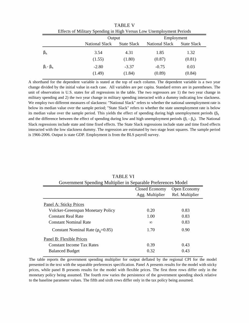
National Slack State Slack National Slack State Slack

βh 3.54 4.31 1.85 1.32

(1.55) (1.80) (0.87) (0.81)

βl ‐ βh -2.80 -3.37 -0.75 0.03

(1.49) (1.84) (0.89) (0.84)

Output Employment

Effects of Military Spending in High Versus Low Unemployment PeriodsTABLE V

A shorthand for the dependent variable is stated at the top of each column. The dependent variable is a two yearchange divided by the initial value in each case. All variables are per capita. Standard errors are in parentheses. Theunit of observation is U.S. states for all regressions in the table. The two regressors are 1) the two year change inmilitary spending and 2) the two year change in military spending interacted with a dummy indicating low slackness.We employ two different measures of slackness: "National Slack" refers to whether the national unemployment rate isbelow its median value over the sample period; "State Slack" refers to whether the state unemployment rate is belowits median value over the sample period. This yields the effect of spending during high unemployment periods (βh

and the difference between the effect of spending during low and high unemployment periods (βl - βh). The National

Slack regressions include state and time fixed effects. The State Slack regressions include state and time fixed effectsinteracted with the low slackness dummy. The regression are estimated by two stage least squares. The sample periodis 1966-2006. Output is state GDP. Employment is from the BLS payroll survey.

Closed Economy Agg. Multiplier

Open Economy Rel. Multiplier

Panel A: Sticky PricesVolcker-Greenspan Monetary Policy 0.20 0.83Constant Real Rate 1.00 0.83Constant Nominal Rate ∞ 0.83

Constant Nominal Rate (ρg=0.85) 1.70 0.90

Panel B: Flexible PricesConstant Income Tax Rates 0.39 0.43Balanced Budget 0.32 0.43

TABLE VIGovernment Spending Multiplier in Separable Preferences Model

The table reports the government spending multiplier for output deflated by the regional CPI for the modelpresented in the text with the separable preferences specification. Panel A presents results for the model with stickyprices, while panel B presents results for the model with flexible prices. The first three rows differ only in themonetary policy being assumed. The fourth row varies the persistence of the government spending shock relativeto the baseline parameter values. The fifth and sixth rows differ only in the tax policy being assumed.

Closed Economy Agg. Multiplier

Open Economy Rel. Multiplier

Panel A: Sticky PricesVolcker-Greenspan Monetary Policy 0.12 1.42Constant Real Rate 7.00 1.42Constant Nominal Rate ∞ 1.42

Constant Nominal Rate (ρg=0.50) 8.73 2.04

Panel B: Flexible PricesConstant Income Tax Rates 0.00 0.30Balanced Budget -0.18 0.30

TABLE VIIGovernment Spending Multiplier in GHH Model

The table reports the government spending multiplier for output deflated by the regional CPI for the modelpresented in the text with the GHH preferences specification. Panel A presents results for the model with stickyprices, while panel B presents results for the model with flexible prices. The first three rows differ only in themonetary policy being assumed. The fourth row varies the persistence of the government spending shock relativeto the baseline parameter values. The fifth and sixth rows differ only in the tax policy being assumed.

Closed Economy Agg. Multiplier

Open Economy Rel. Multiplier

Panel A: Sticky PricesBaseline Model (Complete Markets) 0.20 0.83Incomplete Markets, Locally Financed 0.18 0.84Incomplete Markets, Federally Financed 0.18 0.90

Panel B: Flexible PricesBaseline Model (Complete Markets) 0.39 0.43Incomplete Markets, Locally Financed 0.39 0.41Incomplete Markets, Federally Financed 0.39 0.40

TABLE VIIIGovernment Spending Multipliers in Incomplete Markets Model

The table reports the government spending multiplier for output deflated by the regional CPI for a version of themodel presented in the text with seperable utility in which the only financial asset traded across regions is a non-contingent bond. Panel A presents results for the model with sticky prices, while panel B presents results for themodel with flexible prices.

Output CPI Inflation

Baseline Model (Fixed Capital) 1.42 0.17Firm-Specific Capital Model 1.47 0.15Regional Capital Market Model 0.98 0.11Firm-Specific Capital Model , Flexible Prices 0.25 0.36

Open Economy Relative Multiplier in Models with Variable CapitalTABLE IX

The table reports the open economy relative government spending multiplier for output and CPIinflation for our baseline model with GHH preferences and the two models with variable capital alsowith GHH preferences. Output is deflated by the regional CPI.

Figure I Prime Military Contract Spending as a Fraction of State GDP

0

0.01

0.02

0.03

0.04

0.05

0.06

0.07

0.08

1966 1970 1974 1978 1982 1986 1990 1994 1998 2002 2006

California

National

Illinois

Figure II Prime Military Contracts and Military Shipments

0

5

10

15

20

25

30

35

1966 1970 1974 1978 1982 1986 1990 1994 1998 2002 2006

Billion $ California

Prime Military Contracts

Military Shipments

012345678910

1966 1970 1974 1978 1982 1986 1990 1994 1998 2002 2006

Billion $ Conneticut

0

12

34

56

78

9

10

1966 1970 1974 1978 1982 1986 1990 1994 1998 2002 2006

Billion $ Massachusets

0

5

10

15

20

25

30

1966 1970 1974 1978 1982 1986 1990 1994 1998 2002 2006

Billion $ Texas

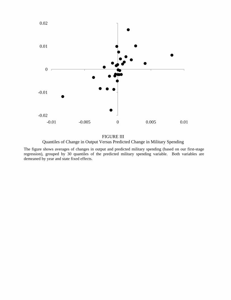
FIGURE III Quantiles of Change in Output Versus Predicted Change in Military Spending

The figure shows averages of changes in output and predicted military spending (based on our first-stage regression), grouped by 30 quantiles of the predicted military spending variable. Both variables are demeaned by year and state fixed effects.

-0.02

-0.01

0

0.01

0.02

-0.01 -0.005 0 0.005 0.01

Figure IV Prices and Real Interest Rates after a Government Spending Shock

The figure plots the relative price level and the relative real interest rate in the two regions for the model with separable preferences after a positive government spending shock to the home region.

-0.10

-0.05

0.00

0.05

0.10

0.15

0.20

0.25

0 5 10 15 20 25 30 35 40 45 50 55 60 65 70 75 80

Price Level

Real Interest Rate

Figure V Consumption and Real Interest Rate after a Government Spending Shock

The figure plots the relative consumption and the relative real interest rate in the two regions for the model with separable preferences after a positive government spending shock to the home region.

-0.25

-0.20

-0.15

-0.10

-0.05

0.00

0.05

0 5 10 15 20 25 30 35 40 45 50 55 60 65 70 75 80

Consumption

Real Interest Rate

Figure VI Output and Consumption after a Government Spending Shock in GHH Model

The figure plots the relative output and consumption in the two regions for the model with GHH preferences after a positive government spending shock to the home region.

-0.50

0.00

0.50

1.00

1.50

2.00

2.50

0 5 10 15 20 25 30 35 40

Output

Consumption

Government Spending