1

Fiscal redistribution around elections when “democracy is not the only

game in town”

Pantelis Kammas a and Vassilis Sarantides

b

a Department of Economics, University of Ioannina, P.O. Box 1186, 45110 Ioannina, Greece.

kammas@cc.uoi.gr

b

Department of Economics, University of Sheffield, 9 Mappin Str, Sheffield S1 4DT, UK.

v.sarantides@sheffield.ac.uk

January 15, 2014

Abstract: This paper examines whether policy intervention around elections affects income

inequality and actual fiscal redistribution. We first develop a simplified theoretical framework

which allows us to examine fiscal redistribution around elections when “democracy is not the

only game in town” and there is a threat of revolution from some groups of agents. Subsequently,

employing data for a panel of 65 developed and developing countries during the period of 1975-

2010 we provide robust empirical evidence of electoral cycles on income inequality and actual

fiscal redistribution in countries characterized as “new democracies”. Moreover, our analysis

suggests that this effect is mainly driven by a political instability channel which induces

incumbents to redistribute resources –through fiscal policy-towards the poorer segments of the

society in order to convince them the “democracy works”. In contrast, inequality and actual

fiscal redistribution are not affected by elections in countries characterized as established

democracies.

JEL: D63, D72, E62

Keywords: elections, new democracy, redistribution, income inequality

Acknowledgments: Without implicating, we wish to thank George Efthyvoulou, Arne Risa Hole, Nasos Roussias,

and seminar participants in the Governance and Participation workshop at the University of Sheffield for valuable

comments and suggestion. The usual disclaimer applies.

2

1. Introduction

Numerous studies on Political Budget Cycles (PBC) suggest that around the election date,

incumbents manipulate policy instruments in order to increase the chances of their re-election.1

A strand of this literature places the spotlight on factors conditioning the occurrence and the

strength of fiscal policy manipulation for electoral purposes (for a literature review on

conditional PBCs, see Klomp and de Haan (2013a)). Starting from Schuknecht (1996) the

relevant literature suggests that fiscal manipulation is more likely in developing countries where

the institutional checks and balances are weaker, allowing for greater political discretion over

policy instruments.2 Shi and Svensson (2006) provide evidence of fiscal expansions around

elections in both developing and developed countries although they show that the effect is far

stronger in developing countries, where information asymmetries between voters and politicians

are more pronounced. Brender and Drazen (2005), on the other hand, argue that PBCs are not

driven by differences in the level of development between countries but instead by differences in

the age of the political regime. More precisely, they suggest that pre-electoral fiscal manipulation

is stronger in countries characterized as “new democracies” because of the voters’ lack of

familiarity with the electoral process.3

Another strand of the literature investigates how pre-electoral manipulation affects the

composition rather than the level of fiscal policy. More precisely, Schuknecht (2000) provides

empirical evidence of pre-electoral manipulation at the national level –in 24 developing

countries- through increases in public investment rather than public consumption. Similar

empirical findings are provided by studies conducted at the local level, which suggest that

around elections authorities expand the level of investment spending (see, e.g., Khemani (2004);

Drazen and Eslava (2010)). The theoretical argument behind these empirical findings is that

capital spending for investment projects can be easily targeted to particular geographical

constituencies, and therefore is able to increase very effectively the political support received by

1 The opportunistic approach was firstly formulated in the traditional model of “political business cycles” of Nordhaus (1975). In

contrast, the partisan approach deals with the behavior of ideologically motivated politicians (see, e.g., Hibbs (1977)). 2 Streb eat al. (2009) support this argument by showing that in non-OECD countries the budget balance falls significantly more in

election years in comparison to what occurs in OECD countries. 3 More recently, Klomp and de Haan (2013b) provided evidence that the occurrence of a PBC is much stronger in developing

counties and “young democracies” as opposed to industrial countries and “old democracies”. However, Efthyvoulou (2012),

based on a sample of 27 European Union members for which fiscal policy is the only remaining instrument that incumbents can

use, provides evidence in favour of a systematic electoral cycle in the level of fiscal policy. It is worth noting, though, that when

Klomp and de Haan (2013c) employ a semi pooled model to allow the impact of elections to vary across countries, they find no

PBC in most countries.

3

the incumbent (see e.g., Drazen and Eslava (2010)). In contrast, Block (2002) and Vergne

(2009) provide empirical evidence that around elections politicians in developing countries shift

the composition of spending towards current expenditure and away from capital expenditure.

Similar findings are also obtained by Katsimi and Sarantides (2012) for a sample of OECD

countries, where policymakers seem to provide immediate benefit to voters through cuts in direct

taxation whereas capital spending decreases. The theoretical justification of these empirical

results dates back to the Rogoff’s (1990) argument, who suggests that electorally motivated

incumbents signal their competence by shifting public policy toward more visible fiscal items

and away from capital expenditure that becomes visible in future periods.4

This paper contributes to the relevant literature basically in two ways. First, it seeks to

investigate the implications of pre-electoral manipulation of fiscal policy on income inequality.

As already mentioned, previous empirical studies have verified that pre-electoral periods exert

significant impact on the size and the composition of government spending (see e.g., Brender

and Drazen (2005); Vergne 2009) as well as on the size and the composition of tax revenues (see

e.g., Persson and Tabellini, 2003; Katsimi and Sarantides, 2012). These changes on fiscal policy

are expected to have vital distributional implications which- to the best of our knowledge- have

not been examined by the relevant literature. To this end, we employ data from Standardized

World Income Inequality Database (SWIID), developed by Solt (2009) which allow us to

investigate the effect of PBC on (i) market income inequality (i.e. Gini coefficient before taxes

and transfers) on (ii) net income inequality (i.e. Gini coefficient after taxes and transfers) as well

as on (iii) actual fiscal redistribution (i.e. the percentage change of Gini indices before and after

transfers and taxes).

Second, our analysis extends the theoretical model of Aidt and Mooney (2014) in order to

develop a simple theoretical framework in which “elections take place in the shadow of

revolution”. This allows us to investigate the differences on the political budget cycles between

countries characterized as “old democracies” (where elections are the one and only common

acceptable political rule) and “new democracies” where the democratic regime is not fully

consolidated and therefore incumbent politicians face a potential threat of revolution from

specific groups of agents (see e.g. Fearon, 2011; Little, 2012; Little et al., 2014). In the latter

4 We note that manipulation of the composition of fiscal policy seems particularly relevant in developed economies, in which the

incumbent may avoid deficit creation due to the fear of voters’ disfavour (see, e.g., Brender and Drazen (2008)).

4

case, incumbent politicians decide pre-electoral fiscal policy by taking into account also the

probability of democratic regime’s collapse and not only their own reelection probability.

Uncertainty concerning the type of the political regime alters in a very fundamental way the pre-

electoral optimal strategy of the incumbent and consequently affects the impact of elections on

the implemented fiscal policy. More precisely, our theoretical model suggests that in “new

democracies” fiscal policy also serves as a device of consolidating democracy and it is not solely

a policy instrument that affects the reelection probability of the incumbent. Thus, in young

democracies pre-electoral fiscal redistribution allocates resources to a broader group of agents

(which also include low-income agents) instead of being strictly targeted to the middle-class that

consist the pivotal group in the “established” ones.5

Our empirical analysis builds on a dataset of 65 developed and developing countries over

the period of 1975-2010. Our main results can be summarized as follows: first, our analysis fails

to provide evidence in favour of an electoral cycle on (i) market income inequality, (ii) net

income inequality and (iii) actual fiscal redistribution for countries characterized as “established

democracies”, irrespective of whether they are developed or developing countries. In contrast,

our analysis provides robust empirical evidence that in countries characterized as “young

democracies” elections exert a positive and highly significant impact on actual fiscal

redistribution. Moreover, our findings suggest that the effect of elections is stronger in young

democracies characterized by relatively higher political instability. This is accordance with the

implications driven from our theoretical framework which suggests that in vulnerable democratic

regimes incumbent politicians allocate resources –through fiscal policy-towards the poorer

segments of the society in order to convince them that “democracy works” and therefore to

mitigate the risk of a potential revolution. Our empirical findings are also in line with previous

studies examining the impact of the political regime’s age on political budget cycles (see e.g.

Brender and Drazen, 2005; 2009, Klomp and de Haan, 2013d).

The rest of the paper is organized as follows. Section 2 introduces the theoretical

framework and formalizes the testable implications of the theoretical model. Section 3 describes

5 Obviously, our theoretical results are in line with those obtained by Brender and Drazen (2005; 2009) although in our model

differences on the political budget cycles between “new” and “old democracies” is driven by the potential threat of revolution

and not from lack of familiarity of the electorate with the democratic electoral process as suggested by them.

5

the data and demonstrates the empirical setup. Section 4 presents the empirical results. Finally

Section 5 summarizes the main points.

2. Theoretical Framework

This section elaborates on the theoretical link between elections and fiscal redistribution so as to

formalize the testable empirical implications driven by the relevant theoretical literature. To this

end, we present a simple theoretical framework adapted from Lohmann (1998) and Aidt and

Mooney (2014) which allows us to examine fiscal redistribution during pre-electoral periods.

We consider an economy populated by three types of individuals: the rich (R) of size δR,

the middle class (M) of size δM and the poor (P) of size δP where we assume that δM > δR+δP and

δR +δM+δP=1. The rich have a fixed income yR, the middle class a fixed income yM and the poor a

fixed income yP where yR>yM >yP during two periods t=1,2. Tax rate (τ) is proportional on

income of each group and it is fixed at a level of in both periods. Elected national

government -in each period- collects tax revenues and runs a balanced government budget by

deciding whether to use given tax revenues in order to finance a lump-sum targeted transfer ( P

t )

that only goes to poor people or a lump-sum transfer ( M

t ) that is directed to the middle class or a

lump-sum transfer ( R

t ) that is directed to the rich group of the individuals. Finally, the

government decides whether to extract resources from public funds by diverting tax revenues to

private income (tr ) for itself. The government budget constraint is P M R

t t t tT T r y where

y is the average income. An election takes place between the two periods.

Citizens’ wellbeing depends on three factors: (i) the budget allocation, (ii) the quality of

the politician running the government and (iii) random events (luck). The utility generated by the

budget allocation and private consumption is

(1 )P P

t P tu y T (1)

(1 )M M

t M tu y T

(2)

(1 )R R

t R tu y T

(3)

6

Quality of governance matters for the citizens because the utility they get from a given

budget allocation increases with the quality of the incumbent politician. The total utility of the

agents is

(1 )P P

t P t t tU y T q (4)

(1 )M M

t M t t tU y T q

(5)

(1 )R R

t R t t tU y T q

(6)

where tq is a quality shock, which determines how competent is the incumbent and t is a

“luck” shock that makes him look more or less competent that may be the case. The

fundamental information assumption of the model is that the voters observe total utility but they

are unable to decompose this into the three sub-components.6 Although, the two shocks are

unobserved, they are both drawn from known distributions. The luck shock ( t ) is drawn

independently in each period and equals to -1/2 (resp. 1/2) with probability P=1/2 (resp. P=1/2).7

The quality shock ( tq ) is a characteristic of the politician and follows a uniform distribution over

1 1,

2 2

.If the politician is getting reelected the quality shock from period 1 also applies to

period 2 whereas if a new politician is elected in period 2 a new quality shock is drawn from the

above mentioned known uniform distribution.

The total utility of the politician is:

1 2ln( ) ( )POL IW r p M r

(7)

6 The underlying assumption is that voters are ill-informed about the finer details of public finance. This is analogous to the

assumption in Lohmann (1998) that voters don observe in direct way the implemented monetary policy. 7 That is the luck shock (μt) follows a Bernoulli distribution with P(-1/2)=P(1/2)=1/2

7

where 0 1 is a discount factor and Ip is the probability that the incumbent is

reelected. The quantity tr denotes rents grabbed in period t=1,2 and M denotes the exogenous

rents from winning the elections.

We solve the model under two alternative political regimes. The first one (that will serve

as benchmark) is an established democratic regime in which “democracy is the only game in

town”. In this case, citizens vote the politician which is – according to their view- the most

competent and then all agents accept the electoral outcome as the sole common political rule. In

such a context, the incumbent politician has incentive to strictly focus on the welfare of the

middle class trying to engineer a pre-election increase in its utility since the latter makes him

appear more competent and consequently increases his probability of reelection. In this case, our

results are similar to those obtained by the relevant theoretical literature (see e.g. Aidt and

Mooney, 2014; Shi and Svensson, 2006; Lohmann, 1998). The second political regime is a “new

democracy” in which “elections take place in the shadow of revolution”. In this case, the

incumbent politician faces a potential threat of revolution from some groups of agents and the

previous described strategy of focusing solely on the welfare of the middle class fails to ensure

staying in office. In such a case, politicians have also to take into account the probability of

survival of the democratic regime per se (except of their own reelection probability) in order to

stay in power. Since the fragility of the democratic regime is related to the welfare of groups

other than the pivotal voter, the optimal strategy for the incumbent is to focus on the welfare of a

broader group of agents.

2.1 Fiscal redistribution when “democracy is the only game in town”.

First, consider the benchmark case of an established democracy. The timing of the events in this

case is as follows: (1) At the beginning of period 1 a balanced budget 1 1 1 1, , ,P M RT T r is

implemented. (2) The two random shocks 1q and 1 are realized. Random shocks are not

observed directly by anyone but all agents are able to observe total utility. (3) At the end of the

first period, elections take place and the voters either re-elect the incumbent politician or elect a

new politician. (4) The winner implements a balanced budget 2 2 2 2, , ,P M RT T r for period 2. (5) A

new luck shock 2 is realized. If the incumbent of the first period was reelected the quality shock

8

from period 1 (i.e. 1q ) carries over to period 2 otherwise a new quality shock 2q is realized. (6)

Finally, total utility is determined and observed by all the agents.

Solving the model with backwards induction, we see that in period 2, the politician has

no incentive to behave well. Therefore, he appropriates the maximum amount of rents

*

2r y implying zero targeted transfers to all alternative groups of agents * * *

2 2 2 0P M RT T .

Equations (4)-(6) imply that voters are clearly better off with a more competent (high q)

politician, as this gives them higher period 2 utility. Thus, they use elections as a mean to

reappoint competent politician and oust incompetent ones, taking into account their observed

utility in period 1 and knowing that the opponents’ expected quality at the elections is ( ) 0E q .8

We now describe how this takes place and how it shapes politician’s incentives in period 1.

2.1.1. The optimal voting behavior and the utility targets.

In order to describe how the politician’s decisions in period 1 affect the probability of re-election

we need to describe optimal voting behavior.

In period 2, since 2r y and 2 2 2 0P M RT T the welfare of agents in the three groups is as

follows:

2 2 2(1 )P

PU y q (8)

2 2 2(1 )M

MU y q

(9)

2 2 2(1 )R

RU y q

(10)

where 2 1 2(1 )I Iq p q p q since if the incumbent of the first period is getting reelected the

quality shock from period 1 ( 1q ) carries over to period 2 whereas if a new politician is elected a

new quality shock ( 2q ) is realized. Since all politicians implement the same post election budget,

the only reason voters care about who gets reelected is that quality varies.

As seen from period 1, the expected quality of the politician elected in period 2 is

8 This is because the quality shock of the opponent is drawn from a uniform distribution which is known to the voters.

9

1 2 1 1 1 2 2 1 1(1 ) ( )I I IE q p E q p E E q p E q (11)

This is because the expected quality of a new politician is zero on average 1 2 2 2 2( ) 0E E q E q .

Thus, the voters want to re-elect the incumbent if and only their estimate of his quality at the end

of the period 1 is positive. That is, if and only if 1 1 0E q . Since in our model δM > δR+δP the

pivotal group of voters is the group of the middle class (M). Thus, we further proceed by

focusing on the preferences of this specific group of agents on the actions of the politician.

More precisely, to form a Bayesian estimate of the expected quality of the incumbent

middle class voters use information on the observed utility of the first period 1

MU and their

knowledge about the equilibrium budget strategy of the incumbent. The equilibrium budget

strategy of the incumbent is 1 1(1 )M M

Mu y T . Subtracting equilibrium budget strategy (1

Mu )

from equation (5) we get:

1 1 1 1 1 1 1 1

M M M MU u T T q q

(12)

where we get the last equality by making use of the fact that at equilibrium 1 1

M MT T . Equation

(12) shows that using their knowledge of the equilibrium, voters can infer the sum of the two

shocks (but they are unable to decompose between these two and therefore to infer the quality of

the politician). A rational voter can solve the resulting signal extraction problem and estimate

that:

2

1 1 1 1 1 12 2( ) ( )

q M M M M

q

E q U u U u

(13)

where is a constant term, 0 1

Based on equation (13) we conclude that the incumbent politician will be reelected if realized

utility of the middle class exceed the budget related utility that the voters are expecting from the

10

incumbent to deliver in equilibrium. That is if and only if 1 1 0M MU u . Using equation (12) we

can restate this criterion as 1 1 1 1

M Mq T T .

Having assumed that 1 follows a Bernoulli distribution with P(-1/2)=P(1/2)=1/2 and

that 1q follows a uniform distribution over 1 1

,2 2

we get that summation 1q + 1 follows a

uniform distribution over 1,1 .

Consequently we get the following probability of reelection as perceived by the incumbent:

1 1

1[1 ( )]

2

M M

Ip T T (14)

Equation (14) shows that reelection probability is increasing in the actual fiscal redistribution

directed to the middle class. This provides an incentive to decide the allocation of tax revenues

such as to increase fiscal redistribution towards this group of individuals.

2.1.2. The budget allocation in equilibrium

Combining equations (7) and (14) with the government budget constraint we conclude that the

equilibrium values for 1 1 1 1, , ,P M RT T r are those that maximize the incumbent inter-temporal

utility:

1 1 1 2

1ln( ) [1 ( )] ( )

2

M M

POLW r T T M r

(15)

subject to the government budget constraint in the first period1 1 1 1

P M RT T r y and the rent

extraction decision of the second period (i.e. *

2r y ). Then, Appendix 2 shows:

11

Proposition 1. The politician generates a rational political budget cycle. The pre-election result

is *

1

2

10

( )

MT yr

,

*

1

2

1

( )r y

r

, * *

1 1 0P R

and the after election result

* * *

2 2 2 0P M RT T and *

2r y .

That is although the politician wants more rents and less fiscal redistribution, in the pre-electoral

period cuts rents and increase fiscal redistribution to the middle class in order to convince pivotal

voters of his quality.

Proposition 2. Pre-electoral increases in transfers targeted to the group of the middle class

* *

1 2

2

1

( )

M MT y Tr

do not change the after tax and transfers Gini coefficients and

therefore do not affect actual fiscal redistribution.

Since pre-electoral increased transfers are solely directed to the middle class and not to the lower

income group of agents, elections fail to affect -after tax and transfers- income inequality and

actual fiscal redistribution.

2.2 Fiscal redistribution when “elections take place in the shadow of revolution”.

In this Section we solve the model for the case of a “new-established democracy”. More

precisely, we assume that in the first years after democratic consolidation, “democracy is not the

only game in town” and citizens have an option to revolt against the incumbent if the later fails

to ensure a minimum amount of competence. Therefore, in this case the democratic regime is not

taken as given and there is a probability of democratic regime’s collapse and consequently

reversal to other forms of governance.

The timing of the events in this case is as follows: (1) At the beginning of period 1 a

balanced budget 1 1 1 1, , ,P M RT T r is implemented. (2) The two random shocks 1q and 1 are

realized. Random shocks are not observed directly by anyone but all agents are able to observe

total utility. (3) At the end of the first period, elections take place and the voters either re-elect

the incumbent politician or elect a new politician. (4) After elections, the citizens decide whether

to revolt or not. More precisely, if the incumbent politician fails to convince the citizens that his

12

quality exceeds a minimum amount of competence, a revolution takes place and the democratic

regime collapses with probability Rp . (5) In period 2, regardless of whether democratic regime

survived or not [in stage 4] the official implements a balanced budget 2 2 2 2, , ,P M RT T r (6) A new

luck shock 2 is realized. If the democratic regime was survived and the incumbent of the first

period was reelected the quality shock from period 1 (i.e. 1q ) carries over to period 2 otherwise a

new quality shock 2q is realized. (7) Finally, total utility is determined and observed by all the

agents.

Solving again the model with backwards induction, we see that in period 2, the official

(whether democratically elected or not) has no incentive to behave well. Therefore, he extracts

the maximum amount of rents *

2r y implying zero targeted transfers to all alternative groups

of agents * * *

2 2 2 0P M RT T T . As in Section 2.1, equations (4)-(6) imply that citizens are clearly

better off with a more competent (high q) politician, as this gives them higher period 2 utility.

Thus, they use elections as a mean to reappoint competent politician and throw out of office

incompetent ones. However, in the case of a “new established democracy” the citizens have one

additional option in order to ensure a minimum amount of competence (i.e. quality q) that is the

option to revolt against the incumbent and to oust him out of office. Now we describe how this

takes place and how it shapes politician’s incentives in period 1.

2.2.1. The optimal voting behavior and the utility targets.

Since δM >δR+δP when elections take place the pivotal group of voters remains the group of the

middle class (M). Following the rationale developed in Section 2.1.1 the criterion of the middle

class to vote for the incumbent is 1 1 0M MU u that concludes to the following probability of

reelection as perceived by the incumbent: 1 1

1[1 ( )]

2

M M

Ip T T . Thus, reelection probability in

a “new established democracy” is identical to that characterized the established ones. More

precisely, the probability of reelection is increasing in the fiscal transfers ( 1

MT ) directed to the

middle class.

13

2.2.2. The threat of revolution.

After elections take place, the citizens from the middle class (M) and the low income (P) groups

decide whether to revolt or not.9 Citizens revolt if and only their estimate of the incumbent

quality at the end of the first period is negative and below a threshold quality level q . That is, if

and only 1 1 0E q q . This condition poses a binding constraint to the incumbent only in the case

of the low income citizens. This is because middle class citizens determine the probability of

reelection through their voting behavior and therefore they demand an even higher (i.e. a

positive) competence at the end of the first period in order to vote for the incumbent.10

Thus, we

focus on the low income group of agents and we examine how the threat of potential revolution

shapes politician’s incentives in period 1.

Low income citizens revolt against the incumbent if and only their estimate of his quality

at the end of the period 1 is negative and below a threshold quality level q , 1 1 0E q q . As in

Section 2.1.1 in order to form a Bayesian estimate of the expected quality citizens rely on the

observed utility of the first period 1

PU and their knowledge about the equilibrium budget strategy

of the incumbent. The equilibrium budget strategy of the incumbent is 1 1(1 )P P

Mu y T .

Subtracting equilibrium budget strategy ( 1

Pu ) from equation (4) we get:

1 1 1 1 1 1 1 1

P P P PU u T T q q

(16)

Equation (16) shows that using their knowledge of the equilibrium, citizens can infer the sum of

the two shocks (but they are unable to decompose between these two and therefore to infer the

quality of the politician). A rational citizen can solve the resulting signal extraction problem and

estimate that:

9 Our assumption that revolution can take place at the end of the first period and only after elections is consistent with a small

albeit growing theoretical literature that treats elections as a public signal of government’s popularity which helps the citizens to

solve potential problems of collective actions and to revolt against the incumbent whenever there is verified a high level of anti-

regime sentiments (see e.g. Fearon, 2011; Little 2012; Little et al. 2014). Moreover, Brender and Drazen (2007) provide

empirical evidence that, in young democracies, the regime is almost three times more likely to collapse in election years than in

non-election years. 10 Note that middle class citizens vote for the incumbent if only their estimate of the incumbent quality at the end of the first

period (1 1E q ) is positive (i.e. if

1 1 0E q ).

14

2

1 1 1 1 1 12 2( ) ( )

q P P P P

q

E q U u U u

(17)

Based on equation (17) we conclude that low income citizens revolt if 1 1( )P PU u q .

Using equation (16) we can restate this criterion as1 1 1 1

P Pqq T T

. Since 1q + 1 follows a

uniform distribution over 1,1 , we get that 1 1

qq

follows a uniform distribution

over 1 ,1q q

. Thus the probability of revolution as perceived by the incumbent is as

follows:

1 1

1[1 ( )]

2

P P

R

qp T T

(18)

that leads to the following probability of democratic regime survival:

1 1

11 [1 ( )]

2

P P

D R

qp p T T

(19)

Equation (19) shows that the probability of democratic regime’s survival is increasing in fiscal

transfers directed to the low income group of individuals ( 1

PT ). Thus, when “elections take place

in the shadow of revolution” incumbent faces an incentive increase fiscal redistribution towards

the poorer agents since in this way he stabilizes the political regime and consequently increases

the probability to stay in office. In other words, in a relatively new democracy focusing solely on

the preferences of the middle class (which remain the pivotal voter when elections are taking

place) is not be enough in order to remain in office since there is a threat of revolution from the

low income group that may lead to political regime switch.

Consequently, the total utility of the politician in the case a “new established” democracy

takes the following form:

15

1 2ln( ) ( )POL D IW r p p M r

(20)

where Ip is the probability of the incumbent to be reelected and Dp the probability of the

democratic regime to survive.

2.2.3. The budget allocation in equilibrium

Combining equations (20), (14) and (19) with the government budget constraint we conclude that

the equilibrium values for 1 1 1 1, , ,P M RT T r are those that maximize the incumbent inter-temporal

utility in the case of a “new established” democracy:

1 1 1 1 1 2

1 1ln( ) [1 ( )] [1 ( )] ( )

2 2

M M P P

POL

qW r T T T T M r

(21)

subject to the government budget constraint in the first period1 1 1 1

P M RT T r y and the rent

extraction decision of the second period (i.e. *

2r y ). Equation (21) shows that in the case of a

“new established democracy” fiscal transfers to the middle class ( 1

MT ) and fiscal transfers to the

low-income group of agents ( 1

PT ) are equally efficient in achieving the purpose of incumbent’s

survival. This is because fiscal transfers directed to the low-income group of agents ( 1

PT ) is a

policy instrument that affects democratic consolidation whereas fiscal transfers directed to the

middle class ( 1

MT ) is a policy instrument that affects re-election probability. Then, Appendix 2

shows:

Proposition 3. The politician generates a rational political budget cycle. The pre-election result

is * *

1 1

2

10

1( )

2

M PT y T

r

,

* *

1 1

2

10

1( )

2

P MT y T

r

,

* * *

1 1 1

M Pr y T T y ,

*

1 0R and the after election result * * *

2 2 2 0P M RT T and *

2r y .

16

That is although the politician wants more rents and less fiscal redistribution, in the pre-electoral

period cuts rents and increase fiscal redistribution at least to the one of the two groups of agents

(i.e. *

1 0MT or *

1 0PT ) in order to convince the citizens of his quality. Obviously, incumbent’s

survival can be obtained through several combinations of *

1

MT and *

1

PT .

Proposition 4. Every combination of *

1

MT and *

1

PT that ensures *

1 0PT directs an amount of

total transfers to the low-income group of agents. In this case pre-electoral increases in transfers

reduce the -after tax and transfers- Gini coefficients and increase actual fiscal redistribution.

Therefore, in the case of “new established democracies” positive pre-electoral transfers to the

low income group of agents ( *

1 0PT ) can be optimal solution for the incumbent. In this case, an

amount of transfers is directed to the low income agents and therefore elections exert a negative

impact on -after tax and transfers- income inequality and a positive impact on actual fiscal

redistribution.

3. Econometric analysis

3.1 Data set and variables

Following previous studies, we measure income inequality using the Gini coefficient index. This

index ranges from a minimum value of zero, indicating that all individuals have the same

income, to a theoretical maximum of one, at which all incomes are concentrated in one person. A

primary concern on research for inequality is data comparability, both over time and across

countries. Our preferred data are obtained by the SWIID, developed by Frederick Solt (Solt

(2009)). The SWIID maximizes the comparability of income inequality statistics for the largest

possible sample of countries and years, namely for 174 countries for as many years as possible

from1960 to 2010. For the construction of the dataset, Solt (2009) employed a custom missing-

data algorithm to standardize Gini estimates from all major existing resources of inequality data

(e.g., Luxembourg Income Study, World Income Inequality database etc). An important

advantage of the SWIID is that it maximizes the comparability of income inequality statistics for

the largest possible sample of countries and years. The SWIID includes Gini estimates for gross

income (before taxes and transfers) as well as net income (after taxes and transfers) denoted as

17

gini_market and gini_net, respectively. Furthermore, the percentage change between gini_market

and gini_net gives us an estimate of fiscal redistribution11

:

it

ititit

Ginitaxpre

GinitaxpostGinitaxpreredist

(22)

An additional advantage of the SWIID is that, potential pre-electoral effects on income

distribution can help us to draw inferences regarding the implemented fiscal policy around

elections. For instance, pre-electoral policies based on targeted transfers to low income groups

potentially can affect gini_net and redist, while public projects that promote public employment,

if targeted to low-income groups, can affect gini_market. Moreover, the SWIID provides

estimates of uncertainty for each observation of the income inequality and redistribution

measures. Closely related to this point, Solt (2009) notes that inequality data are often thin in the

early years included in the SWIID. For this reason, the variable redist is only reported after 1975

for most of the advanced countries and only after 1985 for most countries in the developing

world. Hence, given that the quality of data is significantly improved, we opt for using only

those observations for the variables gini_market and gini_net for which the variable redist is

available.12

It should be stressed that the Political Cycles models assume competitive elections.

Therefore, in our sample we include only those countries for which the variable POLITY2 from

the Polity IV Project receives positive values, and at the same time variables Liec and Eiec from

the Database on Political Institutions (DPI), provided by the World Bank (Keefer (2012)),

receive values equal or higher than 6.13

Following the majority of the empirical literature, we

measure electoral uncertainty by constructing an election dummy (elec) that receives the value of

one in an election year and zero otherwise. It is worth noting that we restrict our attention to

legislative elections for countries with parliamentary political systems and presidential elections

for countries with presidential systems. Election dates were collected from the DPI and

11 This measure is denoted by Solt (2014) as relative fiscal redistribution. Alternatively, if we use the difference between market-

income and net-income Gini-indices that Solt denotes as absolute fiscal redistribution, our results remain essentially the same. 12 It is worth noting that, in Section 4.3, we conduct a battery of robustness checks in order to limit further the uncertainty that is

related to the Gini estimates and be more confident about the precision of our results. 13 A value of 6 indicates that multiple parties did win seats, but the largest party can receive more than 75% of the seats.

However, our sample and results remain essentially the same if we restrict variables Liec and Eiec to receive a value of 7, which

indicates multiparty elections and that the largest party got less than 75% of the seats.

18

complemented, when needed, with information from various sources (e.g., the African Elections

Database).

Moreover, to check for differences between “new” and “established democracies”, based

on the approach of Brender and Drazen (2005), we consider the first four elections after a shift to

a democratic regime, indicated by the first year of a string of uninterrupted positive POLITY

values, as elections held in a “new democracy”. We expect that in “new democracies”, it is more

likely to find systematic electoral patterns on income inequality/redistribution for two reasons.

First, according to the above-mentioned study, “new democracies” are more prone to policy

manipulation, since incumbents might be rewarded at the polls if they can “mislead”

inexperienced voters to attribute the good economic conditions to their competency. Second, we

expect that, in “new democracies”, checks and balances are weaker, allowing for greater political

discretion over policy instruments. Thus, we separate binary indicator elec into variables

elec_new and elec_old, for elections in “new democracies” and in “old/established democracies”,

respectively. In our case, among the 362 elections in the sample, 109 elections were held in “new

democracies”.14

Another interesting issue concerning this literature is the timing of elections. As argued

by Berument and Heckelman (1998), the timing of elections may not be exogenous to

government policy but is chosen strategically by the incumbent when economic conditions are

favourable, raising issues of a reverse causation in our specification. On the other hand, early

elections may be also called due to a deterioration of economic conditions that may create a

majority for replacing the government. In order to address the issue of potential endogeneity of

electoral procedures, we follow the approach of Brender and Drazen (2005) to distinguish pre-

determined elections. More precisely, we look at the constitutionally determined election interval

and take as predetermined those elections that are held during the expected year of the

constitutionally fixed term. Hence, we split electoral indicator elec_new into elec_new_pred

(resp. elec_new_endog) for predetermined (resp. endogenous) elections held in “new

democracies”, and elec_old into elec_old_pred (resp. elec_old_endog) for predetermined (resp.

14 Moreover, pre-electoral manipulation of fiscal policy, and thus income distribution, may depend significantly on the nature of

the constitutional rules. As outlined by the relevant literature, politicians in proportional and parliamentary democracies are more

prone to promote broad-based policies, such as welfare spending, whereas in majoritarian and presidential ones, this holds for

geographically targeted expenditures (see, e.g., Milesi-Ferretti et al. (2002); Persson and Tabellini (2002)). Hence, electoral

cycles may differ between proportional and majoritarian systems or presidential and parliamentary governments. It is worth

noting, though, that when we split our electoral indicator to account for these differences, the results (available upon request) did

not produce any significant electoral effect on income inequality/redistribution.

19

endogenous) elections in “old democracies”. In our case, among the 109 (253) elections held in

“new democracies” (“old democracies”) in the sample, 87 (177) elections are classified as

predetermined. Our unbalanced cross-country time series dataset includes observations for 65

countries over the period of 1975-2010 (see Appendix 1).15

In turn, we consider in our empirical analysis a number of explanatory control variables

that we expect to affect income inequality and redistribution. More precisely, we include in the

set of explanatory variables GDP per capita (gdppc) and its squared term (gdppc^2), obtained

from Penn World Tables, to test for the hump-shaped relation between economic development

and inequality, as described by Kuznets (1955). Moreover, from the same database we obtain an

index of human capital per person (human capital), based on years of schooling (Barro and Lee

(2013)) and returns to education (Psacharopoulos (1994)). We expected an increase in the human

capital index to be negatively related to income inequality (see e.g., Li et al. (1998)). In addition,

in our analysis we include a number of demographic variables obtained from World Bank's

World Development Indicators (WDI).

More precisely, we employ the dependency ratio of the population (dependency) that is

measured as the percentage of the population younger than 15 years or older than 64 to the

number of people of working age between 15 and 64 years. This variable allows us to control for

demographic influences on the structure of social spending and fiscal redistribution (see, e.g.,

Galasso and Profeta, 2004; von Weizsacker, R., 1996). The next control is population density

(population density) defined as the population divided by land area in square kilometers. A larger

share of population density ensures economies of scale in the provision of the public good and

therefore higher fiscal redistribution for given level of spending (see e.g. Alesina and Wacziarg,

1998). Yet, the model includes the inflation rate (inflation), because low-income households are

likely to be relatively more vulnerable to price increases than others (see, e.g., Albanesi 2007).

Furthermore, we use the KOF Index of Economic Globalisation (global), developed by Dreher

(2006), to test the potential effects of economic globalisation on fiscal redistribution and income

inequality (see e.g. Rodrik, 1997; 1998). Finally, we control for regional fixed effect through

dummies identifying countries in East-Asia Pacific, Eastern Europe and Central Asia, Latin

America, Middle-East and North Africa, North America and Western Europe, the Pacific and the

15 The sample size was restricted by the availability of income inequality data as well as the competitiveness of elections for

those countries and years for which income inequality data are available. Moreover, it is worth noting, that when we restrict the

sample to those countries that we have more than 10 observations results (available upon request) remain unaffected.

20

Caribbean and Sub-Saharan Africa. A complete list of all variables used in our estimations is

provided in the Data Appendix.16

3.2. Empirical Specification

The basic specification we use to analyze the impact of elections on income inequality and fiscal

redistribution is in the following form:

ittiitititit elecaYaY 110 (23)

where Yit stands for the dependent variables that are of interest for income inequality

(gini_market and gini_net) and fiscal redistribution (redist) in country i and year t; elec is the

indicator we use to capture the influence of elections; Z is the vector of country-specific socio-

economic control variables that we expect to affect income inequality and redistribution; μi and λt

are unobserved country and time-specific effects, respectively, and εit is the error term.

In line with many previous studies, we include the lagged dependent variable Yit-1 on the

right-hand side of our estimated equation, since income inequality may exhibit a great deal of

persistence for which one has to control (see, e.g., Chong et al. (2009); Amendola et al. (2013)).

A problem that arises from this specification, though, is that regressions produce high

autoregressive coefficients near or above 0.9, suggesting that we might well be faced with

nonstationarities. If our dependent variable is not stationary, we are faced with spurious

relationships when that variable is entered on the right-hand side of the equation. Hence, before

proceeding in our estimations, we carry out the Maddala and Wu (MW) (1999), Choi (2001),

Levin et al. (LLC) (2002) and Im et al. (IPS) (2003) tests to check for the presence of a unit root.

The LLC test assumes that the autoregressive coefficient is common across all cross sections,

whereas the other tests are less restrictive, allowing for individual unit roots processes so that the

persistence parameters may vary across cross-sections. The null hypothesis in all panel unit root

tests is that all series are non-stationary against the alternative that at least one series in the panel

is stationary. As can be seen in Table 1, when a constant and a trend are included, we have clear

indications that variables gini_market, gini_net and redist are non-stationary. For this reason, we

16 We have also attempted to include in our model a series of other control variables, such as population size, population density,

population growth, foreign aid, voter turnout, variables on political constraints, and others. However, none of these variables had

a significant effect on income inequality/redistribution, and due to other concerns as well (correlation of control variables,

reduction of sample size), we do not include them in our estimations. Results are available upon request.

21

apply the same panel unit root test to the first-differenced data. The trend drops out in that case

and therefore is not included in the panel unit-root-test regressions in first differences. The

results indicate that we can reject the null of non-stationarity at the 1% significance level.

[Table 1, here]

A common approach for dealing with non-stationary data is to take first differences in

order to proceed with a dynamic specification in differences (see, e.g., Mechtel and Potrafke

(2013)). Hence, we end up estimating the following equation:

ittitititit elecaYaY 110 (24)

where we first difference our dependent variable and the covariates of our model − all measured

initially in levels − with the exception of the electoral dummy variable. This implies that we put

more structure in the data for the identification of the election effect. It is worth noting, though,

that the inclusion of a lagged dependent variable introduces a potential bias by not satisfying the

strict exogeneity assumption of the error term εit. One solution could probably be the application

of dynamic panels (e.g., Arellano and Bond (1991); Blundell and Bond (1998)). The problem

that arises is that these estimators yield consistent estimates in small T large N panels. In our

case, we have 65 countries, and when we split our sample between developed and developing

countries, these numbers decrease to 22 and 43 countries, respectively. Still, as it is analyzed in

the literature, the estimated bias of this formulation is of order 1/T, where T is the time length of

the panel, even as the number of countries becomes large (see, among others, Nickell (1981)).

The average time series length of our panel is around 22, 29 and 18 for the whole sample, the

developed and developing countries, respectively, making the bias probably negligible. It is

worth noting by taking first differences we eliminate time-invariant country effects, but not time-

fixed effects. Hence, we estimate equation (24) using a dynamic OLS model with time fixed

effects.17

However, in the next section that we check the robustness of our results, splitting even

17 The F-test results presented in our tables indicate that time-fixed effects are in general significant, and therefore they are

included in the regressions. The qualitative results in all regressions do not significantly change when we exclude year effects.

22

further our sample and reducing the average time series length below 12, we implement also the

bias-corrected Least Squares Dummy variable estimator (LSDVc).

4. Results

4.1 Baseline Results

We start our analysis by estimating Equation (24), using the set of control variables described

above. Regarding the lagged dependent variable, our results reveal positive and statistically

significant coefficients, in the strong majority of our estimates, suggesting that income inequality

display a great deal of persistence. Moreover, we get some weak evidence that GDP per capita is

positively related to Δredist (Δgini_market) in the group of developed (developing) countries.

Furthermore, the squared term of GDP per capita, namely Δgdppc^2, has a negative, though not

robust effect on Δredist (Δgini_market) in the case of developed (developing) countries.

Interestingly enough, the human capital indicator (Δhc) has a statistically significant effect only

when regressed against net income inequality in Table 8, while we find no effect of the age

dependency (Δdependency) on income inequality and fiscal redistribution.18

On the other hand,

the coefficient of variable Δpopulation_density, when the OLS model is applied, is positive when

significantly related to market inequality and fiscal redistribution. Next, as expected, the variable

Δinflation is positively and significantly related to net inequality in the general specification of

Table 2. This result, though, does not seem to be robust on the one hand, and on the other hand,

when we split our sample between developed and developing countries, it seems to be driven by

the case of developing countries. Finally, the variable Δglobal has a positive (negative), though

not robust, effect on net income inequality (fiscal redistribution) in developed countries.

[Table 2, here]

Moving one step forward, in columns (1)-(3) of Table 2 we estimate the effect of elections on

income inequality (Δgini_market and Δgini_net) and fiscal redistribution (Δredist), using the

18 It should be noted that the qualitative results remain essentially the same after dropping these two variables from our

regressions.

23

simple pre-electoral indicator. Our results indicate that the variable elec is negative and

significantly related to the variable Δgini_net at the 10% level. Hence, we get some weak

evidence that around elections net income inequality decreases. In columns (4)-(6), we separate

binary indicator elec into variables elec_new and elec_old, for elections held in “new” and “old

democracies”, respectively. Our results show that the variable elec_new is negatively related to

net income inequality at the 1% level.19

Given the insignificant coefficient of variable elec_new

when related to Δgini_market in column (4), we have a clear indication that in “new

democracies” incumbents intervene pre-electorally to redistribute income to low-income groups.

Indeed, in column (6), the coefficient of elec_new is positively related to Δredist at the 5% level,

which implies that in “new democracies” office-motivated incumbents engage in pre-electoral

manipulation to redistribute income to the poorer members of the society. Next, in columns (7)-

(9) we proceed into a four-way split of our electoral indicator to distinguish between pre-

determined and endogenous elections that were held either in “new” or in “old democracies”.

The significant coefficient of the variable elec_new_pred, suggests that only in “new

democracies” and during predetermined electoral campaigns, held during the expected year of

the constitutionally fixed term, incumbents adopt policies that generate fiscal redistribution.

Next, in Table 3 we replicate the regressions of columns (7)-(9) of Table 2, after splitting

the sample between developed and developing countries. We separate the sample because

according to the literature, apart from the issue of the age of the democracy, the level of

development can be a crucial determinant for the pre-electoral intensity of fiscal manipulation

(see e.g., Streb and Torrens (2013), Klomp and de Haan (2013b)). More specifically, in

developing countries checks and balances can be weaker, and informational asymmetries

regarding the competence level of the incumbent (a crucial assumption of PBC models) more

pronounced, making more likely the adoption of intense pre-electoral policies. In the case of

developed countries, it has been argued that the electorate can monitor more easily the elected

officials, and punish those who engage in pre-electoral manipulation (see e.g., Brender and

Drazen (2008)). On the other hand, it is true that incumbents in developed countries have a

greater variety of policy instruments on their disposal. This availability gives them the

opportunity to disguise a possible pre-electoral intervention on the one hand, in order to avoid

19 As already mentioned, following the approach of Brender and Drazen (2005), we consider the first four elections after a shift to

a democratic regime, as elections held in a “new democracy”. Alternatively if we reduce the number to three the effect of

elections becomes stronger, while the opposite holds if we increase the number of elections held in a “new democracy” to five.

24

the punishment of the electorate, and on the other hand, it makes highly likely an impact on

income inequality and/or redistribution measures.

The division of the sample reveals that the result for fiscal redistribution (Δredist), is

driven by the experience of less-developed countries. More precisely, the electoral indicator

suggests for developing countries an increase in Δredist of 0.87% during predetermined elections

in “new democracies”. Given that the mean value of redist in the sample of developing countries

is 9.87%, the estimate implies that, on average, the percentage reduction in market income

inequality due to taxes and transfers increases by 8.8% during predetermined elections in “new

democracies”.

[Table 3, here]

Our empirical findings are in line with the results driven from our theoretical model as

well as with previous studies examining similar issues (see e.g. Brender and Drazen, 2005;

2009). More precisely, our analysis suggests that in relatively vulnerable democratic regimes

incumbent politicians allocate resources –through fiscal policy-towards the poorer segments of

the society whereas in the case of well established democracies our analysis fails to verify impact

of elections on fiscal redistribution. According to our model this difference can be explained by

taking into account that in new democracies elections take place “in the shadow of revolution”

from low income groups and therefore fiscal policy serves as a device of consolidating

democracy. Our findings are also in accordance with Brender and Drazen (2008; 2009) who

suggest that pre-electoral shift in fiscal policy in “new democracies”, does not improve re-

election prospects and conclude that incumbent politicians provide benefits mostly because they

seek to provide a signal that “democracy works” and therefore to prevent a reversion to

autocracy.20

The same authors provide evidence that, in young democracies, the regime is almost

three times more likely to collapse in election years than in non-election years.

On the other hand, results for developed countries deviate significantly from what we get

for developing countries. More precisely, although we get a negative effect of elec_new_pred on

market inequality (Δgini_market), which contributes to the significant reduction of net

inequality, fiscal redistribution does not seem to be affected pre-electorally. In is worth noting,

20 According to Brender and Drazen (2009), in a “new democracy”, antidemocratic elites are not the only ones that may pose a

threat to the democratic regime. The support by the masses cannot always be taken for granted and electoral policies can serve to

shore up mass support.

25

though, that we cannot make strong inferences about this result, because we have only 8 electoral

observations for this variable. However, this result may indicates that the level of development of

the public sector in developed countries, allows them to intervene pre-electorally using a variety

of different policy instruments. In particular, government intervention may not come solely from

transfers, but also from public projects that can potentially decrease market inequality (see, e.g.,

Alesina et al. (2000)). Moreover, empirical evidence suggests that, in developed and established

democracies, incumbents intervene pre-electorally through cuts in direct taxation and increases

in public consumption (see e.g., Efthyvoulou (2012); Katsimi and Srantides (2012)).

Interestingly enough, though, this intervention does not seem to generate fiscal redistribution or

to affect income inequality. This empirical finding is in accordance to the theoretical argument of

Olson (1982) that long periods of democracy are associated with formation and accumulation of

interest groups and lobbies that demand redistribution in favour of them and away from more

disadvantaged citizens in order to ensure political support to the government.

4.2. Sensitivity analysis

In this section we inquire into the robustness of the analytical results obtained in Tables 3, by re-

estimating the regressions under various modifications. First, we re-estimate equation (24) after

splitting our sample into “new” and “old democracies”. Second, we repeat regressions of Table 3

using an alternative electoral indicator that allows us to control for differences in election dates

across as well as within countries. Finally, we repeat regressions to ensure that the results of

Table 3 are not influenced by outlier observations.

4.2.1. Alternative Specification

As a first step of the sensitivity analysis, instead of dividing the electoral dummy variable

between “new” and “old democracies”, we proceed to split our sample. More precisely, in

columns (1)-(3) of Table 4 we restrict our sample only to those observations that a country is

considered as an “old democracy”. Next, we re-run equation (24) for “old democracies” after

splitting the sample between developed and developing countries, in columns (4)-(6) and (7)-(9),

respectively. Moreover, in columns (10)-(12) we keep only those observations that a country is

considered a “new democracy”, while in columns (13)-(15) we keep in our sample only “new

26

democracies” in developing countries.21

As already discussed in section 2.2, the inclusion of a

lagged dependent variable on the right-hand-side of the equation introduces a potential bias of

order 1/T, where T is the time length of the panel (see, among others, Nickell (1981)). The

average time series length of our panel until know was above 18 and the bias is probably

negligible. However, in this section that the average length of the panel decreases in some cases

below 12, we opt for using the LSDVc estimator as proposed by Kiviet (1995) and extended by

Bruno (2005) to unbalanced panels.22

[Table 4, here]

As can be seen, our results in Table 4 seem to verify those obtained in Table 3. More precisely, it

seems that in “old democracies”, irrespective of whether they are developed or developing

counties, income inequality and fiscal redistribution are not affected during electoral campaigns.

More importantly, results verify that only in “new democracies” and during predetermined

electoral campaigns incumbents adopt policies that generate fiscal redistribution.

4.2.2. Weighted electoral indicator

Until now, in order to capture the effect of elections, we followed the majority of the relevant

literature, and we included in our regressions an election dummy (elec) that receives the value of

one in an election year and zero otherwise. It is important to note that this indicator is not

affected by the specific timing of elections. This might be problematic, because if elections take

place early in the year, then the dummy variable may be capturing primarily post-electoral

effects. One way to deal with this issue is to construct a pre-election indicator (preel) that takes

the value of x/12, with x denoting the month the election is held, in order to directly control for

differences in election dates across as well as within countries (see, e.g., Franzese 2000). In order

to reproduce regressions in Table 3, we proceed into a four-way split of variable preel. More

precisely, we split indicator preel into preel_new_pred (preel_new_end) and preel_old_pred

21 Unfortunately, we do not have enough observations to perform regressions for “new democracies” in developed economies. 22 We use the Arellano-Bond (1991) as the first step estimator, whereas we undertake 200 repetitions of the procedure to

bootstrap the estimated standard errors. The qualitative results, though, remain unaffected when we apply the Anderson and

Hsiao (1982) or the Blundell and Bond (1998) models as first-step estimators or even when we apply more repetitions to estimate

the standard errors.

27

(preel_old_end), for predetermined (endogenous) elections in “new” and “old democracies”,

respectively.

[Table 5, here]

Regarding the effect of elections on inequality and redistribution, the qualitative results

presented in Table 5 remain essentially the same as those depicted in Table 3. More precisely,

our previous finding that fiscal redistribution (Δredist) increases only during predetermined

elections held in “new democracies” continues to hold.

4.2.3. Testing for outliers

As a final step, we perform three checks to ensure that the results presented in Table 3 are not

influenced by outlier observations. First, to control for the effect of individual outliers, we use

Cook's distance that measures the effect of deleting a given observation based on each

observation's residual in the regression and its leverage in the estimation process. Hence,

according to the rule of thumb, we re-estimate regressions without observations with a Cook’s

distance larger than 4/n (where n the number of observations). As can be seen, Cook’s distance

identified 32 to 40 outlier observations in the various specifications. In Tables 6 that we re-

estimate our regressions after dropping the identified outlier observations the statistical

significance of the main variables of interest remain unaffected. Moreover, as expected, the R-

squared of the estimated equations has significantly improved by the exclusion of the outliers.

[Table 6, here]

Second, as already mentioned, the SWIID maximizes the comparability of available

income inequality data, but incomparability remains and it is reflected in the standard errors

reported for each observation of variables gini_market, gini_net and redist. The provision of

standard errors is an additional advantage of the SWIID, because it allows us to take into account

the largest part of the remaining uncertainty of inequality data estimates. Hence, in Table 7, in

order to increase further the reliability of our results, we choose to exclude from regressions 10%

of the observations that variables gini_market, gini_net and redist are associated with the higher

28

standard errors.23

The results that are reported in Tables 7 and confirm our previous finding

about the positive impact of elections held in “new democracies” on fiscal redistribution.

[Table 7, here]

Finally, in Table 8 we estimate our preferred specifications excluding the ex-Soviet Union

countries. Given the profound restructuring of these countries’ societies and economies during

the period of democratisation, which probably differs from other democratizations observed in

our sample, we attempt to assess the importance of this group of countries for our results. Hence,

in columns (1)-(3) of Table 8 we choose to exclude the ex-Soviet Union countries from the full

sample of 65 countries, as well as from the group of developing countries in columns (4)-(6). As

can be seen in Table 8, our results for the effect of elections on fiscal redistribution do not seem

to be driven by the experience of the ex-Soviet Union countries.

[Table 8, here]

4.3. Regime’s stability and fiscal redistribution around elections

So far our results indicate that the age of the regime is a crucial determinant for the shape of

fiscal policy around elections. More specifically, during the first four elections of a newly

established democratic regime, fiscal manipulation seems to generate fiscal redistribution. On the

other hand, pre-electoral manipulation after the consolidation of the democratic regime does not

seem to provide any distributional implications. It seems that the vulnerability of the democratic

regime in the first years after the transition is directly related to this result. More precisely,

according to Brender and Drazen (2009), in the first years after the transition, antidemocratic

elites are not the only threat to the newly established regime. The support by the masses cannot

always be taken for granted, and electoral policies can serve to shore up mass support. The same

authors provide evidence that in “new democracies” the regime is almost three times more likely

to collapse in election years than in non-election years. Hence, fiscal redistribution to low-

23 Additionally, if we drop from our sample the three Sub-Saharan Africa countries, where the precision of the estimates for the

Gini-indices and fiscal redistribution measures may not be that accurate, our results (available upon request) remain unaffected.

29

income groups can serve as a signal that “democracy works” and prevent a reversion to

autocracy at a time of high vulnerability. On the other hand, after some years where the regime

consolidates, although evidence suggests that elected officials manipulate fiscal policy, the effect

on fiscal redistribution disappears.

In this section we attempt to provide additional evidence that the vulnerability of the regime,

which so far has been measured by the age of the democracy, is of paramount importance for the

observed pro-poor pre-electoral policies. Ideally, in our analysis, we would prefer to use

measures for the public attitudes towards democracy based on the World Value Survey

(Inglehart et al. 2004). Unfortunately, though, for the most relevant to our research questions of

this survey (e.g., having a democratic political system) we have only 3 observations per country

from 1994 onwards. As an alternative, we use measures of state violence that are provided at the

Social, Political, and Economic Event Database (SPEED), collected by Nardulli et al. (2012) at

the University of Illinois. The database includes daily observations for a range of variables (e.g,

coups, anti-regime protests etc), which we collapse into simple counts per country-year. From

the alternatives provided, we choose the variables state repression and state violence as the two

most relevant for our purpose. Hence, in order to identify the potential effect of regime’s stability

on the relationship between the elections and fiscal redistribution we modify equation (3) in the

following way:

0 1 1 2

3

*

it it it

it t it

Y a Y a elec elec state repression

state repression

(25)

0 1 1 2

3

*

it it it

it t it

Y a Y a elec elec state violence

state violence

(26)

where the variables state repression and state violence enter in equation (25) and (26), on their

own and interacted with the variable elec. More precisely, in Table 9, where the dependent

variable is fiscal redistribution (Δredist), we interact the four-way split electoral indicator with

the two alternative measures of political instability. In columns (1) and (4) we use the whole

sample of countries, while in columns (2), (5) and (3), (6) the groups of developed and

developing countries, respectively.

30

[Table 9, here]

The results obtained are very interesting. As can be seen, the variable Δstate repression is

insignificantly related to fiscal redistribution in all estimates, while Δstate violence is negatively

related to fiscal redistribution in the specification for the whole groups of countries in column

(4). Moreover, when we split the sample between developed and developing countries, none of

the electoral variables, or the interacted terms, are statistically significant for the case of

developed countries. Nonetheless, for developing countries when we interact state repression

and state violence with the electoral indicators, evidence is supportive for the effect of pre-

electoral instability on the shape of fiscal policy. More specifically, in column (3) although we

find no evidence of fiscal redistribution around endogenous elections in “new democracies”,

when we interact the variable elec_new_end with state repression the effect becomes positive

and statistically significant. Interestingly enough, for the same group of countries, it seems that

state violence is an important determinant of fiscal redistribution not only in “new” but in “old”

democracies as well, as indicated by the statistically significant coefficients of the variables

elec_new_pred*Δstate violence and elec_old_pred*Δstate violence. Hence, as expected, in the

first years after the transition to the democratic regime, when the elected officials face

turbulences around elections, they shift fiscal policy towards poorer segments of the society in

order to stabilize the regime. The fact that we get an identical result for “old democracies” in

developing countries, might prove that the path to consolidation in many cases is not completed

after the end of the first years of the democratic transition.

5. Conclusions

This paper examines whether policy intervention around elections affects income inequality and

actual fiscal redistribution. Building on the theoretical model of Aidt and Mooney (2014) we

develop a simplified theoretical framework which allows us to examine fiscal redistribution

around elections when “democracy is not the only game in town” and there is a threat of

revolution from the low income groups of agents. Our analysis suggests that in relatively

vulnerable democratic regimes -where fiscal policy also serves as a device of consolidating

31

democracy- incumbent politicians allocate resources to a broader group of agents (which include

low-income agents) during the pre-electoral periods. In contrast, in relatively stable democratic

regimes fiscal transfers are strictly targeted to the middle class that consists the pivotal group of

voters in “old democracies”.

Subsequently, employing data for a panel of 65 developed and developing countries

during the period of 1975-2010 we provide robust empirical evidence that in countries

characterized as “young democracies” elections exert a positive and highly significant impact on

actual fiscal redistribution. Moreover, our findings suggest that the effect of elections is stronger

in young democracies characterized by relatively higher political instability. In contrast, our

analysis fails to provide evidence in favour of an electoral cycle on (i) market income inequality,

(ii) net income inequality and (iii) actual fiscal redistribution for countries characterized as

“established democracies”, irrespective of whether they are developed or developing countries.

32

Appendix 1: List of countries

Country

Developed

economy

Transition

economy

“New

democracy”

Years included in the sample (as

“New Democracy”)

Number of elections

(as “New Democracy”)

Argentina √ 1987-2010 (1987-2003) 5 (4)

Armenia √ √ 1995-2008(1995-2008) 3(3)

Australia √ 1975-2010 13

Austria √ 1985-2010 8

Bangladesh √ 1992-2010 (1992-2010) 2(2)

Belgium √ 2001-2010 3

Bolivia √ 1991-2004 (1991-1997) 4(2)

Brazil √ 1987-2009 (1987-2002) 5(4)

Bulgaria √ √ 1993-2010 (1993-2006) 4 (3)

Canada √ 1975-2010 10

Chile √ 1990-2009 (1990-2009) 4(4)

Colombia 1987-2009 5

Costa Rica 1987-2009 5

Czech Republic √ √ 1995-2010(1995-2006) 5(4)

Denmark √ 1978-2010 11

Dominican Rep. √ 1988-2009(1988-1994) 6(2)

Ecuador √ 1989-2009(1989-1996) 6(2)

El Salvador √ 1987-2008 (1987-1994) 4(2)

Estonia √ √ 1997-2010(1997-2003) 3(2)

Finland √ 1975-2010 8

France √ 1975-2010 8

Germany √ 1991-2010 5

Guatemala √ 1987-2006(1987-1999) 5(4)

Honduras √ 1991-2010(1991-1993) 5(1)

Hungary √ √ 1991-2010(1991-2002) 5(3)

India 1987-2005 6

Indonesia √ 1999-2010(1999-2010) 3(3)

Ireland √ 1982-2009 7

Israel 1978-2005 8

Italy √ 1977-2010 9

Japan √ 1977-2010 11

Korea √ √ 1987-2010(1987-2000) 6(4)

Latvia √ √ 1993-2010(1993-2002) 5(3)

Lithuania √ √ 1994-2010(1994-2010) 4(3)

Luxemburg 2001-2010 2

Malaysia 1989-2005 4

Mexico √ 1994-2010(1994-2010) 3(3)

Moldova √ √ 1993-2010(1993-2009) 5(4)

Nepal √ 1992-2002(1992-2002) 2(2)

Netherlands √ 1975-2010 11

New Zealand √ 1978-2007 9

Norway √ 1978-2010 8

Panama √ 1989-2010(1989-2004) 5(4)

Paraguay √ 1992-2010(1992-2000) 5(3)

Peru √ 1987-2010(1987-1995) 5(2)

Philippines √ 2002-2009(2002-2009) 1(1)

Poland √ √ 1990-2010(1990-2004) 4(3)

Portugal √ √ 1982-2010(1982-1985) 9(2)

Romania √ √ 1992-2010(1992-2004) 5(4)

Russia √ √ 1994-2008(1994-2008) 4(4)

Senegal √ 2000-2006(2000-2006) 1(1)

Slovak Rep. √ √ 1994-2010(1995-2002) 5(4)

Slovenia √ √ 1992-2010(1994-2004) 5(4)

South Africa 1987-2006 5

Spain √ √ 1982-2010(1982-1986) 8(2)

Sweden √ 1977-2010 10

Switzerland √ 1982-2010 7

Thailand 1987-2004 3

Trinidad and Tobago 1987-2005 5

Ukraine √ √ 1994-2008(1994-2008) 3(3)

United Kingdom √ 1975-2010 8

United States √ 1975-2010 8

Uruguay √ √ √ 1987-2010(1987-2004) 5(4)

Venezuela 1987-2008 4

Zambia √ 1992-2005(1992-2005) 2(2)

33

Appendix 2

Proposition 1. The politician generates a rational political budget cycle. The pre-election result

is *

1

2

10

( )

MT yr

,

*

1

2

1

( )r y

r

, * *

1 1 0P R

and the after election result

* * *

2 2 2 0P M RT T and *

2r y .

Proof.

In period 2, the politician has no incentive to behave well. Therefore, he extracts the maximum

amount of rents *

2r y implying zero targeted transfers to all alternative groups of

agents * * *

2 2 2 0P M RT T .

In period 1, the incumbent decides optimally 1

P , 1

MT , 1

RT and 1r by maximizing equation (15)

subject to the government budget constraint in the first period (i.e. 1 1 1 1

P M RT T r y ) and the

rent extraction decision of the second period (i.e. *

2r y ). Equation (15) shows that 1

PT and 1

RT

implies solely costs from the point of view of the incumbent. Therefore, in the absence of any

cost benefit trade off, optimal decision is * *

1 1 0P R .

Taking the first order derivative with respect to 1

M , we have:

2

1 1 1

1( )

P M Rr

y T T T

which for given * *

1 1 0P R concludes to *

1

2

1

( )

MT yr

which is positive for 1

( )y

y

.

Finally, from the government budget constraint in the first period (i.e. 1 1 1 1

P M RT T r y ) we

take *

1

2

1

( )r y

r

34

Proposition 2. Pre-electoral increases in transfers targeted to the group of the middle class

* *

1 2

2

1

( )

M MT y Tr

do not change the after tax and transfers Gini coefficients and

therefore do not affect actual fiscal redistribution.

Proof.

By definition the –after tax and transfers- Gini coefficient in period 2 (after the elections) equals

to:

2 ,2 ,2( ) ( )p R R R P P MG s s

where the δ’s denote the proportions of the three groups and the s’s denote the –after taxes and

transfers-income shares of the rich and the poor in the second period.

Similarly the –after tax and transfers-Gini coefficient in period 1 (before the elections) equals to:

1 ,1 ,1( ) ( )p R R R P P MG s s

where the δ’s denote the proportions of the three groups and the s’s denote the –after taxes and

transfers-income shares of the rich and the poor in the first period.

Obviously, since ,1 ,2R Rs s and ,1 ,2P Ps s (i.e. the –after taxes and transfers-income shares of the

rich and the poor do not change from period 1 to period 2), 1 2G G . Therefore, in the pre-

electoral period income inequality remains constant 0G .

Proposition 3. The politician generates a rational political budget cycle. The pre-election result

is * *

1 1

2

10

1( )

2

M PT y T

r

,

* *

1 1

2

10

1( )

2

P MT y T

r

,

* * *

1 1 1

M Pr y T T y ,

*

1 0R and the after election result * * *

2 2 2 0P M RT T and *

2r y .

Proof.

35

In period 2, the politician has no incentive to behave well. Therefore, he extracts the maximum

amount of rents *

2r y implying zero targeted transfers to all alternative groups of

agents * * *

2 2 2 0P M RT T .

In period 1, the incumbent decides optimally1

P ,1

MT ,1

RT and 1r by maximizing equation (21)

subject to the government budget constraint in the first period (i.e. 1 1 1 1

P M RT T r y ) and the

rent extraction decision of the second period (i.e. *

2r y ). Equation (21) shows that 1

RT

implies solely costs from the point of view of the incumbent. Therefore, in the absence of any

cost benefit trade off, optimal decision is *

1 0R .

Then, taking the first order derivatives with respect to 1

P and 1

MT we have:

2

1 1 1

1 1( )

2P M Rr

y T T T

which for given *

1 0R concludes to * *

1 1

2

1

1( )

2

M PT y T

r

and

2

1 1 1

1 1( )

2P M Rr

y T T T

which for given *

1 0R concludes to * *

1 1

2

1

1( )

2

P MT y T

r

Finally, from the government budget constraint in the first period (i.e. 1 1 1 1

P M RT T r y ) we

take * * *

1 1 1

M Pr y T T which is smaller than *

2r for any positive value of *

1

MT or *

1

PT

Proposition 4. Every combination of *

1

MT and *

1

PT that ensures *

1 0PT directs an amount of

total transfers to the low-income group of agents. In this case pre-electoral increases in transfers

reduce the -after tax and transfers- Gini coefficients and increase actual fiscal redistribution.

Proof.

By definition the –after tax and transfers- Gini coefficient in period 2 (after the elections) equals

to:

2 ,2 ,2( ) ( )p R R R P P MG s s

36

where the δ’s denote the proportions of the three groups and the s’s denote the income shares of

the rich and the poor in the second period.

Similarly the –after tax and transfers-Gini coefficient in period 1 (before the elections) equals to:

1 ,1 ,1( ) ( )p R R R P P MG s s

where the δ’s denote the proportions of the three groups and the s’s denote the –after taxes and

transfers-income shares of the rich and the poor in the first period.

It can be easily verified that when * *

1 2 0P PT we have ,1 ,2P Ps s (i.e. the –after taxes and

transfers- income shares of the poor increases in period 1 compared to period 2) and

consequently 1 2G G . In other words, in the pre-electoral period income inequality decreases,

0G .

37

Data Appendix: variable descriptions, descriptive statistics and data sources Variable Description Obs. Mean SD Min Max Source

gini_market Gini coefficient of gross household

market(pre-tax, pre-transfer)

income

1425 44.745 6.574 28.563 69.954 Solt (2009) ,

Standardized World

Income Inequality Database (SWIID)

Δ gini_market Change in Gini coefficient of gross

household income

1425 0.127 1.316 -8.646 7.294 SWIID

gini_net Gini coefficient of household

disposable (post-tax, post-transfer)

income

1425 35.860 10.012 19.700 65.721 SWIID

Δ gini_net Change in Gini coefficient of

household disposable (post-tax,

post-transfer) income

1425 0.056 0.897 -5.685 5.452 SWIID

redist Percentage reduction of Gini

coefficient before and after the

fiscal redistribution (i.e. before and after taxes and transfers)

1425 20.105 16.814 -20.701 59.907 SWIID

Δredist Change in percentage reduction of

Gini coefficient before and after the fiscal redistribution (i.e. before

and after taxes and transfers).

1425 0.054 1.701 -12.390 12.756 SWIID

elec Dummy variable that receives the value 1 in the election year and 0

otherwise.

1425 0.255 0.436 0 1 Keefer (2012), Database of Political Institutions

(DPI)

elec_new Dummy variable that receives the value 1 for elections held in “new

democracies” and 0 otherwise.

1425 0.077 0.267 0 1 DPI

elec_old Dummy variable that receives the

value 1 for elections held in “old

democracies” and 0 otherwise.

1425 0.178 0.382 0 1 DPI

elec_new_pred Dummy variable that receives the

value 1 for predetermined

elections held in “new democracies” and 0 otherwise.

1425 0.062 0.241 0 1 DPI

elec_new_endog Dummy variable that receives the

value 1 for endogenous elections held in “new democracies” and 0

otherwise.

1425 0.015 0.123 0 1 DPI

elec_old_pred Dummy variable that receives the value 1 for predetermined

elections held in “old

democracies” and 0 otherwise.

1425 0.124 0.329 0 1 DPI

elec_old_endog Dummy variable that receives the

value 1 for endogenous elections

held in “old democracies”and 0 otherwise.

1425 0.055 0.228 0 1 DPI

preel_new_pred Indicator variable that receives

value (x/12) in the election year, with x the months before election,

for predetermined elections held in

“new democracies” and 0 otherwise.

1425 0.037 0.160 0 1 DPI

preel_new_endog Indicator variable that receives

value (x/12) in the election year, with x the months before election,

for endogenous elections held in

“new democracies” and 0 otherwise.

1425 0.010 0.086 0 1 DPI

preel_old_pred Indicator variable that receives

value (x/12) in the election year, with x the months before election,

for predetermined elections held in

“old democracies” and 0 otherwise.

1425 0.072 0.212 0 1 DPI

preel_old_endog Indicator variable that receives

value (x/12) in the election year, with x the months before election,

for endogenous elections held in

1425 0.034 0.156 0 1.083 DPI

38

“old democracies” and 0

otherwise.

Liec Legislative index for electoral

competitiveness.

1425 6.974 0.191 6.000 7.000 DPI

Eiec Executive index for electoral competitiveness.

1425 6.974 0.191 6.000 7.000 DPI

gdppc Real GDP per capita income 1425 16.986 12.500 0.736 80.231 Penn World Tables 8

(PWT)

Δgdppc Change in real GDP per capita

income

1425 0.333 0.657 -5.814 4.934 PWT

gdppc^2 Real GDP per capita income squared

1425 444.663 627.043 0.542 6437.068 PWT

Δgdppc^2 Change in real GDP per capita

income squared

1425 15.279 49.568 -894.607 676.467 PWT

hc Index of human capital per person 1425 2.710 0.455 1.404 3.619 PWT

Δhc Change in index of human capital

per person

1425 0.017 0.015 -0.031 0.084 PWT

dependency Population under the age of 14 as a

share of total population (%)

1425 56.139 12.017 37.589 97.765 World Bank

Development indicators

(WDI) online

Δdependency Change in population under the

age of 14 as a share of total

population (%)

1425 -0.454 0.559 -2.354 1.425 WDI online

population

density

Population divided by land area in

square kilometers (% )

1425 122.993 150.577 1.847 1160.990 WDI online

population

density

Change in urban population as a share of total population (% )

1425 1.035 2.304 -2.799 19.547 WDI online

inflation Inflation rate 1425 0.355 2.782 -0.235 68.369 WDI online

Δinflation Change in inflation rate 1425 -0.058 2.949 -64.570 39.090 WDI online

global KOF index of economic

globalization

1425 63.472 16.880 9.863 98.877 Dreher (2006)

Δglobal Change in KOF index of economic

globalization

1425 0.841 2.284 -11.071 19.396 Dreher(2006)

state repression Intensity of state repression 1142 1.114 3.111 0.000 31.600 Social, Political, and Economic Event

Database (SPEED)

Δ state

repression

Change in intensity of state repression

1142 -0.148 3.305 -32.100 22.700 SPEED

state violence Intensity of state violence 1142 2.793 14.858 0.000 313.200 SPEED

Δ state violence Change in intensity of state violence

1142 -0.067 16.878 -275.300 313.200 SPEED

39

References

Adit S., Veiga J., & Veiga G. (2011). Election Results and Opportunistic Policies: A New Test of

the Rational Political Business Cycle Model, Public Choice, 148 (1-2), 21-44.

Aidt, T. S., Mooney, G., (2014). Voting suffrage and the political budget cycle: evidence from

the London Metropolitan Boroughs 1902-1937. Journal of Public Economics 112, 53-71

Albanesi, S. (2007). Inflation and inequality, Journal of Monetary Economics, 54(4), 1088-1114.

Alesin a, A., Baqir, R., & Easterly W. (2000). Redistributive Public Employment, Journal of

Urban Economics, (48)2, 219-241.

Alesina, A. & Wacziarg, R. (1998). Openness, country size and government. Journal of Public

Economics, 69 (3): 305-321.

Amendola, A., & Easaw J., & Savoia, A. (2013). Inequality in developing economies: the role of

institutional development, Public Choice, 155(1), 43-60.

Anderson, W., & Hsiao, C. (1982). Formulation and estimation of dynamic models using panel

data, Journal of Econometrics, 18(1), 47-82.

Arellano, M., & Bond, S. (1991). Some tests of specification for panel data: Monte Carlo

evidence and an application to employment equations. Review of Economic Studies, 58(2),

277-297.

Barro, R., & Lee, J. (2013). A new data set of educational attainment in the world, 1950–2010,

Journal of Development Economics, 104, 184-198.

Bergh, A., Nilsson, T. (2010). Do liberalization and globalization increase income inequality?

European Journal of Political Economy, 26(4), 488-505.

Berument, H., & Froyen, R. (1998). Potential information and target variables for UK monetary

policy, Applied Economics, 30(4), 449-463.

Block, S. (2002). Elections, electoral competitiveness, and political budget cycles in developing

countries. Harvard University CID Working Paper No. 78.

Blundell, R., & Bond, S. (1998). Initial conditions and moment restrictions in dynamic panel

data models, Journal of Econometrics, 87(1), 115-143.

Brender, A., & Drazen A. (2005). Political budget cycles in new versus established democracies.

Journal of Monetary Economics, 52(7), 1271-1295.

Brender, A., & Drazen A. (2007). Why is Economic Policy Different in New Democracies?

Affecting Attitudes. NBER Working Paper No. 13457

Brender, A. & Drazen A. (2008). How do budget deficits and economic growth affect reelection

prospects? Evidence from a large panel of countries. American Economic Review, 98(5),

2203-2220.

Brender, A., & Drazen A. (2009). Consolidation of New Democracy, Mass Attitudes, and

Clientelism. American Economic Review, 99(2), 304-309.

Bruno, G. (2005). Approximating the bias of the LSDV estimator for dynamic unbalanced panel

data models, Economics Letters, 87(3), 361-366.

Choi, I. (2001). Unit root tests for panel data, Journal of International Money and Finance,

20(2), 249-272.

Chong, A., Gradstein, M., & Calderon, C. (2009). Can foreign aid reduce income inequality and

poverty? Public Choice, 140(1), 59–84.

Deaton, A. (1997). The Analysis of Household Surveys—A Microeconometric Approach to

Development Policy. The John Hopkins Univ. Press, Baltimore

Drazen, A., Elsava, M., (2010): Electoral manipulation via voter-friendly spending: Theory and

evidence, Journal of Development Economics, 92:1, 39--52.

40

Dreher, A. (2006). Does Globalization Affect Growth? Empirical Evidence from a new Index.

Applied Economics, 38(10), 1091–1110.

Efthyvoulou, G. (2012). Political budget cycles in the European Union and the impact of

political pressures. Public Choice, 153, 295–327.

Fearon, J., (2011). Self-Enforcing Democracy. Quarterly Journal of Economics 126(4),1661-

1708.

Franzese, R. J. (2000). Electoral and partisan manipulation of public debt in developed

democracies, 1956-1990. In Strauch, R., & Jürgen von Hagen (Eds.), Institutions, politics

and fiscal policy (pp. 61-83). Dordrecht: Kluwer Academic Press.

Galasso, V., & Profeta, P., (2004). Lessons for an Aging Society: the Political Sustainability of

Social Security Systems. Economic Policy, 63-115

Heckelman, J. C. and Berument, H. (1998). Political business cycles and endogenous elections.

Southern Economic Journal, 64(4), 987–1000.

Hibbs, D. A. (1977). Political parties and macroeconomic policy. American Political Science

Review, 71(4), 467-487.

Im, K. S., Pesaran, H., & Shin, Y. (2003). Testing for unit roots in heterogeneous panels, Journal

of Econometrics, 115(1), 53-74.

Katsimi M. & Sarantides V. (2012). Do elections affect the composition of fiscal policy in

developed, established democracies, Public Choice, 151(1), 325-362.

Keefer, P. (2012). Database on Political Institutions: changes and variable definitions, The World

Bank.

Khemani, S. 2004. “Political cycles in a developing economy: Effect of elections in the Indian

states.” Journal of Development Economics 73(1): 125-154.

Kiviet, J. F. (1995). On bias, inconsistency, and efficiency of various estimators in dynamic

panel data models. Journal of Econometrics, 68(1), 53-78.

Klomp, J., De Haan, J. (2013a). Conditional political budget cycles: a review of recent evidence,

Public Choice, 157(3-4), 387-410.

Klomp, J., De Haan, J. (2013b). Do political budget cycles really exist?, Applied Economics,

45(3), 329-341.

Klomp, J., De Haan, J. (2013c). Political budget cycles and election outcomes. Public Choice,

157(1), 245-267.

Klomp, J., De Haan, J. (2013d). Popular protest and political budget cycles: A panel data

analysis, Economics Letters, 120(3), 516-520.

Kuznets, S. (1955). Economic growth and income inequality, American Economic Review, 45(1),

1-28.

Levin, A., Lin, C.-F., & Chu, C.-S. J. (2002). Unit root tests in panel data: asymptotic and finite-

sample properties, Journal of Econometrics, 108(1), 1-24.

Li, H., Squire, L., & Zou, H.-F. (1998). Explaining international and intertemporal variations in

income inequality. Economic Journal, 108(446), 26–43.

Little, A., (2012). Elections, Fraud, and Election Monitoring in the Shadow of Revolution.

Quarterly Journal of Political Science 7(3),249-283.

Little, A., Tucker, J., LaGatta, T., (2014). Election, Protest and alternation of power. Mimeo

Lohman, S., (1998). Rationalizing the political business cycle: a workhorse model Economics

and Politics, 10 (1), 1–17.

Maddala, S., & Wu, S. (1999). A comparative study of unit root tests with panel data and new

simple test, Oxford Bulletin of Economics and Statistics, 61(S1), 631-652.

41

Mechtel M. & Potrafke, N. (2013). Electoral cycles in active labor market policies, Public

Choice, 156(1), 181-194.

Meltzer, A. & Richard, S. (1981). A rational theory of the size of the government, Journal of

Political Economy, vol. 89(5), pp. 914–27.

Milesi-Ferretti, G. M., Perotti, R., & Massimo, R. (2002). Electoral systems and public spending.

The Quarterly Journal of Economics, 117(2), 609-657.

Nardulli, P., Leetaru, K. & Hayes, M. (2011). Event Data, Civil Unrest and the Social, Political

and Economic Event Database (SPEED) Project: Post World War II Trends in Political

Protests and Violence. Paper presented at the Annual meeting of the International Studies

Association, Quebec.

Nickell, S. J. (1981). Biases in dynamic models with fixed effects. Econometrica, 49(6), 1417-

1426.

Nordhaus, W. D. (1975). The political business cycle. Review of Economic Studies, 42(2), 169-

190.

Olson, M., (1982). The rise and decline of nations: Economic growth, stagflation, and social

rigidities. Yale University Press. NewYork.

Persson, T., & Tabellini G. (2003). The economic effect of constitutions. Cambridge: MIT Press.

Psacharopoulos, G. (1994). Returns to investment in education: A global update, World

Development, 22(9), 1325-1343.

Rodrik, D., (1997). Has globalization gone to far? Washington D.C.: Institute for International

Economics.

Rodrik, D., (1998). Do more open economies have bigger governments ? The Journal of

Political Economy, 106(5): 997-1032.

Rogoff, K. (1990). Equilibrium political budget cycles. American Economic Review, 80(1), 21-

36.

Schneider, C. J. (2010). Fighting with one hand tied behind the back: political budget cycles in

the West German states. Public choice, 142(1), 125-150.

Schuknecht, L. (1996). Political business cycles and fiscal policies in developing countries.

Kyklos, 49(2), 155-170.

Shi, M., & Svensson J. (2006). Political budget cycles: do they differ across countries and why?

Journal of Public Economics, 90(8-9), 1367-1389.

Solt, F. (2009). Standardizing the world income inequality database. Social Science Quarterly

90(2), 231-242.

Solt, F. (2014). The Standardized World Income Inequality Database. Working Paper. SWIID

Version 5.0. October 2014.

Streb, J., Lema, D., & Torrens, G. (2009). Checks and Balances on Political Budget Cycles:

Cross Country Evidence, Kyklos, 62(3), 425-46.

Streb, J. M., & Torrens, G. (2013). Making rules credible: divided government and political

budget cycles. Public Choice, 156(3-4), 703-722.

Veiga, L., & Veiga, F. (2007). Political business cycles at the municipal level. Public Choice,

131(1), 45-64.

Vergne, C. (2009). Democracy, elections and allocation of public expenditures in developing

countries. European Journal of Political Economy, 25(1), 63-77.

von Weizsäcker R. (1996). Distributive implications of an aging society, European Economic

Review, 40 (3-5), 729-746.

42

Table 1. Panel Unit root tests (H0: unit root)

Variables

LLC IPS ADF- Fisher Chi-square ADF-Choi Z-stat

Constant Constant and

Trend

Constant Constant and

Trend

Constant Constant and

Trend

Constant Constant and

Trend

gini_market -1.952**

(0.025)

-0.318

(0.375)

1.701

(0.955)

0.473

(0.689)

116.379

(0.626)

153.433**

(0.028)

1.759

(0.961)

0.986

(0.838)

Δgini_market -10.505***

(0.000)

- -8.867***

(0.000)

- 305.895***

(0.000)

- -7.397***

(0.000)

-

gini_net -2.354***

(0.009)

-0707

(0.239)

1.214

(0.887)

1.7001

(0.955)

128.125

(0.334)

110.296

(0.767)

1.207

(0.886)

1.957

(0.974)

Δgini_net -3.125***

(0.001)

- -6.414***

(0.000)

- 271.299***

(0.000)

- -6.673***

(0.000)

-

redist -5.389***

(0.000)

-0.827

(0.204)

-3.565***

(0.000)

-0.416

(0.338)

183.299***

(0.000)

149.287**

(0.047)

-2.885***

(0.002)

-0.295

(0.383)

Δredist -5.622***

(0.000)

- -8.133***

(0.000)

- 342.399***

(0.000)

- -8.379***

(0.000)

-

Notes: The “Δ” prefix of a variable indicates that the first differences were taken. Figures without parenthesis are test statistics and those inside parentheses are respective probabilities. *** denotes significance at 1% level, ** denotes significance at 5% level and * denotes significance at 10% level. Results are reported for a lag length of 1, but are not sensitive to this choice.

43

Table 2. Elections and fiscal redistribution: basic findings (1) (2) (3) (4) (5) (6) (7) (8) (9)

Dependent variable: Δgini_market Δgini_net Δredist Δgini_market Δgini_net Δredist Δgini_market Δgini_net Δredist

elec -0.038 -0.088* 0.132 - - - - - - (0.07) (0.04) (0.09) elec_ new - - - -0.020 -0.247*** 0.631** - - - (0.13) (0.09) (0.26) elec_old - - - -0.046 -0.018 -0.088 - - - (0.07) (0.04) (0.08) elec_new_pred - - - - - - 0.049 -0.268*** 0.853*** (0.12) (0.10) (0.30) elec_new_endog - - - - - - -0.281 -0.164 -0.204 (0.34) (0.24) (0.36) elec_old_pred - - - - - - -0.035 -0.015 -0.025 (0.08) (0.05) (0.09) elec_old_endog - - - - - - -0.071 -0.024 -0.230 (0.18) (0.08) (0.25) ΔYt-1 0.220** 0.191** 0.179** 0.220** 0.194** 0.180*** 0.222*** 0.192** 0.183*** (0.08) (0.09) (0.07) (0.08) (0.09) (0.07) (0.08) (0.09) (0.07) Δgdppc 0.149 0.036 0.166 0.149 0.034 0.177 0.143 0.035 0.154 (0.09) (0.08) (0.12) (0.09) (0.08) (0.12) (0.09) (0.08) (0.12) Δgdppc^2 -0.001 -0.000 -0.002* -0.001 -0.000 -0.002* -0.001 -0.000 -0.002* (0.00) (0.00) (0.00) (0.00) (0.00) (0.00) (0.00) (0.00) (0.00) Δhc -0.006 -2.182 2.773 -0.001 -2.221 2.906 0.003 -2.220 2.947 (2.57) (2.03) (2.50) (2.57) (2.05) (2.51) (2.58) (2.05) (2.53) Δdependency 0.128 0.069 0.075 0.128 0.068 0.077 0.127 0.068 0.074 (0.09) (0.08) (0.10) (0.09) (0.07) (0.10) (0.09) (0.07) (0.11) Δpopulation_density 0.047* 0.006 0.075*** 0.046* 0.008 0.070*** 0.045* 0.008 0.066*** (0.02) (0.02) (0.02) (0.02) (0.02) (0.02) (0.02) (0.02) (0.02) Δinflation 0.019 0.025* -0.018 0.019 0.026* -0.020 0.018 0.026* -0.023 (0.02) (0.01) (0.02) (0.02) (0.01) (0.02) (0.02) (0.01) (0.02) Δglobal 0.029 0.027** -0.012 0.029 0.027** -0.011 0.029 0.027** -0.011 (0.02) (0.01) (0.03) (0.02) (0.01) (0.03) (0.02) (0.01) (0.03) R2 0.131 0.132 0.086 0.131 0.135 0.094 0.132 0.135 0.099 N 1421 1421 1421 1421 1421 1421 1421 1421 1421 Avg. time series

length 21.9 21.9 21.9 21.9 21.9 21.9 21.9 21.9 21.9

Notes: The “Δ” prefix of a variable indicates that the first differences were taken. All regressions include time and regional fixed effects. Robust

standard errors, clustered by country, in parentheses. *** denotes significance at 1% level, ** denotes significance at 5% level and * denotes

significance at 10% level.

44

Table 3. Elections and fiscal redistribution: Developed vs. Developing countries Developed countries Developing countries

(1) (2) (3) (4) (5) (6)

Dependent variable: Δgini_market Δgini_net Δredist Δgini_market Δgini_net Δredist

elec_new_pred -0.790** -0.734* 0.051 0.087 -0.244** 0.873***

(0.33) (0.38) (1.79) (0.11) (0.10) (0.29)

elec_new_endog -0.332 -0.159 -0.198 -0.213 -0.175 -0.152

(0.26) (0.15) (0.40) (0.34) (0.24) (0.44)

elec_old_pred -0.019 0.000 -0.031 -0.024 0.028 -0.039

(0.09) (0.07) (0.11) (0.13) (0.10) (0.18)

elec_old_endog 0.010 0.038 -0.257 -0.184 -0.145 -0.123

(0.23) (0.09) (0.33) (0.27) (0.17) (0.36)

ΔYt-1 0.339*** 0.352*** 0.254*** 0.138 0.129 0.154

(0.07) (0.07) (0.06) (0.11) (0.10) (0.09)

Δgdppc 0.116 -0.018 0.218 0.449* 0.226 0.229

(0.13) (0.09) (0.14) (0.24) (0.25) (0.40)

Δgdppc^2 -0.001 0.000 -0.002* -0.012* -0.006 -0.005

(0.00) (0.00) (0.00) (0.01) (0.01) (0.01)

Δhc 2.732 0.839 4.497 -2.918 -5.157 1.719

(3.02) (1.29) (4.26) (3.96) (3.36) (3.62)

Δdependency 0.144 0.016 0.152 0.070 0.049 0.046

(0.10) (0.07) (0.12) (0.12) (0.12) (0.15)

Δpopulation_density 0.003 0.001 0.006 0.067*** 0.014 0.089***

(0.03) (0.02) (0.04) (0.02) (0.02) (0.02)

Δinflation 0.541 0.487 -0.529 0.018 0.027** -0.027

(2.87) (1.80) (1.64) (0.02) (0.01) (0.02)

Δglobal 0.036 0.046* -0.075** 0.027 0.022 0.002

(0.05) (0.02) (0.03) (0.02) (0.01) (0.03)

R2 0.191 0.193 0.145 0.146 0.167 0.101

N 637 637 637 784 784 784

Avg. time series length 28.9 28.9 28.9 18.2 18.2 18.2 Notes: set Table 2

45

Table 4. Elections and fiscal redistribution: “New” vs. “Old” democracies in Developed and Developing countries “Old Democracies” Developed economies “Old

Democracies”

Developing economies “Old

Democracies”

“New democracies” Developing Economies “New

democracies”

(1) (2) (3) (4) (5) (6) (7) (8) (9) (10) (11) (12) (13) (14) (15)

Dependent variable: Δgini_market Δgini_net Δredist Δgini_market Δgini_net Δredist Δgini_market Δgini_net Δredist Δgini_market Δgini_net Δredist Δgini_market Δgini_net Δredist

elec_pred -0.003 -0.003 -0.013 -0.023 -0.008 -0.023 0.020 0.007 0.006 0.045 -0.232 0.822** 0.094 -0.205 0.908***

(0.12) (0.06) (0.11) (0.14) (0.08) (0.16) (0.13) (0.10) (0.16) (0.20) (0.15) (0.33) (0.21) (0.16) (0.34)

elec_endog -0.016 0.010 -0.193 0.007 0.042 -0.281 -0.138 -0.081 -0.163 -0.324 -0.237 -0.326 -0.361 -0.278 -0.314

(0.05) (0.09) (0.17) (0.17) (0.10) (0.20) (0.26) (0.21) (0.33) (0.37) (0.27) (0.59) (0.42) (0.31) (0.65)

ΔYt-1 0.384*** 0.344*** 0.359*** 0.383*** 0.379*** 0.299*** 0.258*** 0.219*** 0.460*** -0.044 0.003 0.043 -0.043 -0.004 0.066

(0.04) (0.03) (0.03) (0.05) (0.05) (0.05) (0.06) (0.06) (0.06) (0.06) (0.06) (0.05) (0.06) (0.06) (0.06)

Δgdppc 0.024 -0.036 0.117 0.036 -0.082 0.216 0.616* 0.250 0.611 0.186 0.342 -0.258 0.412 0.420 0.086

(0.13) (0.07) (0.14) (0.21) (0.12) (0.24) (0.36) (0.30) (0.45) (0.63) (0.47) (1.01) (0.64) (0.47) (1.02)

Δgdppc^2 -0.000 0.000 -0.001 -0.000 0.001 -0.001 -0.016 -0.006 -0.018 -0.012 -0.016 0.006 -0.030 -0.024 -0.022

(0.00) (0.00) (0.00) (0.00) (0.00) (0.00) (0.01) (0.01) (0.01) (0.03) (0.02) (0.04) (0.03) (0.02) (0.05)

Δhc 0.335 -1.123 3.239 3.165 0.835 6.507 -3.357 -5.066 1.260 -5.807 2.232 -15.572 -6.560 3.840 -21.418

(0.61) (2.15) (3.94) (4.42) (2.44) (5.11) (4.95) (4.05) (6.26) (8.37) (6.18) (13.28) (9.92) (7.30) (15.78)

Δdependency -0.024 -0.019 -0.082 0.054 -0.018 0.055 -0.184 -0.040 -0.174 0.582** 0.616*** -0.163 0.573* 0.638*** -0.241

(0.14) (0.07) (0.14) (0.17) (0.09) (0.20) (0.22) (0.18) (0.27) (0.28) (0.21) (0.45) (0.30) (0.22) (0.47)

Δpopulation_density 0.019 -0.006 0.059 0.025 -0.005 0.077 0.061 -0.004 0.092 -0.509*** 0.066 -0.868*** -0.490*** 0.090 -0.843***

(0.02) (0.04) (0.08) (0.12) (0.07) (0.14) (0.10) (0.08) (0.12) (0.19) (0.14) (0.30) (0.18) (0.13) (0.29)

Δinflation -0.048 0.038 -0.097 1.584 1.156 -0.326 0.228 0.266 -0.051 0.008 0.018 -0.025 0.007 0.017 -0.029

(0.13) (0.19) (0.35) (2.53) (1.40) (2.92) (0.53) (0.43) (0.66) (0.02) (0.01) (0.03) (0.02) (0.01) (0.02)

Δglobal 0.036 0.036** -0.023 0.049 0.054** -0.067 0.030 0.023 0.001 -0.010 0.000 -0.012 -0.005 0.002 -0.008

(0.06) (0.01) (0.03) (0.04) (0.02) (0.05) (0.02) (0.02) (0.03) (0.03) (0.02) (0.05) (0.03) (0.02) (0.05)

N 973 973 973 604 604 604 368 368 368 440 440 440 412 412 412

Avg. time series

length 18.2 18.2 18.2 29.5 29.5 29.5 10.9 10.9 10.9 11.3 11.3 11.3 11.6 11.6 11.6

Notes: The “Δ” prefix of a variable indicates that the first differences were taken. LSDVc estimator using Arellano-Bond (1991) for initial bias correction. All regressions include time fixed effects. Standard errors bootstrapped with 200 replications, are reported in parentheses. *** denotes significance at 1% level, ** denotes significance at 5% level and * denotes significance at 10% level.

46

Table 5. Elections and fiscal redistribution: Alternative timing of elections Developed countries Developing countries

(1) (2) (3) (4) (5) (6)

Dependent variable: Δgini_market Δgini_net Δredist Δgini_market Δgini_net Δredist

preel_new_pred -1.696 -2.264** 2.180 0.113 -0.320** 1.181***

(1.14) (0.98) (5.57) (0.18) (0.15) (0.46)

preel_new_endog -0.398 -0.232 -0.077 -0.382 -0.239 -0.348

(0.39) (0.21) (0.51) (0.34) (0.26) (0.52)

preel_old_pred 0.051 0.028 0.044 -0.014 0.019 -0.053

(0.14) (0.08) (0.17) (0.17) (0.15) (0.19)

preel_old_endog -0.058 0.144 -0.621 -0.348 -0.155 -0.527

(0.29) (0.14) (0.37) (0.46) (0.26) (0.57)

ΔYt-1 0.338*** 0.353*** 0.250*** 0.137 0.128 0.151

(0.07) (0.07) (0.06) (0.10) (0.11) (0.09)

Δgdppc 0.110 -0.018 0.208 0.451* 0.223 0.245

(0.13) (0.09) (0.14) (0.25) (0.25) (0.41)

Δgdppc^2 -0.001 0.000 -0.002* -0.012* -0.006 -0.006

(0.00) (0.00) (0.00) (0.01) (0.01) (0.01)

Δhc 2.687 0.841 4.366 -2.954 -5.159 1.642

(3.07) (1.30) (4.25) (3.94) (3.38) (3.61)

Δdependency 0.147 0.014 0.169 0.068 0.054 0.027

(0.10) (0.07) (0.12) (0.12) (0.12) (0.15)

Δpopulation_density -0.001 0.002 -0.005 0.067*** 0.014 0.088***

(0.03) (0.02) (0.03) (0.02) (0.02) (0.02)

Δinflation 0.574 0.555 -0.611 0.019 0.026* -0.025

(2.87) (1.78) (1.59) (0.02) (0.01) (0.02)

Δglobal 0.036 0.046* -0.074** 0.027 0.023 0.001

(0.05) (0.02) (0.03) (0.02) (0.01) (0.03)

R2 0.190 0.196 0.151 0.147 0.166 0.099

N 637 637 637 784 784 784

Avg. time series length 28.9 28.9 28.9 18.2 18.2 18.2 Notes: set Table 2

47

Table 6. Elections and fiscal redistribution: Excluding outlier observations Developed countries Developing countries

(1) (2) (3) (4) (5) (6)

Dependent variable: Δgini_market Δgini_net Δredist Δgini_market Δgini_net Δredist

elec_new_pred -0.615** -1.018*** -0.314 0.115 -0.073 0.408** (0.26) (0.10) (0.19) (0.10) (0.07) (0.20) elec_new_endog -0.158 -0.181 0.255 -0.131 -0.022 -0.251 (0.13) (0.13) (0.22) (0.19) (0.16) (0.25) elec_old_pred -0.068 -0.005 0.084 0.009 0.080 -0.037 (0.09) (0.04) (0.09) (0.09) (0.06) (0.09) elec_old_endog -0.002 0.022 -0.144 -0.021 -0.153 -0.011 (0.15) (0.05) (0.17) (0.15) (0.14) (0.14) ΔYt-1 0.422*** 0.372*** 0.371*** 0.261*** 0.294*** 0.239*** (0.04) (0.04) (0.04) (0.06) (0.05) (0.06) Δgdppc 0.036 -0.056 0.169 0.172 0.049 0.294 (0.10) (0.06) (0.11) (0.19) (0.18) (0.27) Δgdppc^2 -0.001 0.001 -0.002** -0.004 -0.000 -0.005 (0.00) (0.00) (0.00) (0.01) (0.00) (0.01) Δhc 2.132 1.514 1.195 -3.146 -1.811 2.083 (2.67) (1.39) (2.48) (3.30) (1.95) (2.88) Δdependency 0.084 -0.003 0.132 -0.015 0.095 0.139 (0.07) (0.05) (0.09) (0.11) (0.08) (0.12) Δpopulation_density 0.016 0.003 0.021 -0.009 0.013 0.058*** (0.03) (0.01) (0.03) (0.02) (0.01) (0.02) Δinflation 0.842 0.305 -0.810 0.002 0.014 -0.011 (2.45) (1.18) (1.21) (0.00) (0.01) (0.01) Δglobal 0.009 0.023 -0.055* 0.020 0.011 0.024 (0.02) (0.02) (0.03) (0.02) (0.01) (0.02) R2 0.327 0.284 0.284 0.246 0.267 0.173 N 605 599 606 747 744 744

Avg. time series length 27.5 27.2 27.5 17.4 17.3 17.3 Notes: set Table 2

48

Table 7. Elections and fiscal redistribution: Excluding 10% of obs. with the higher uncertainty Developed countries Developing countries

(1) (2) (3) (4) (5) (6)

Dependent variable: Δgini_market Δgini_net Δredist Δgini_market Δgini_net Δredist

elec_new_pred -1.149*** -0.711* -1.323*** -0.014 -0.245* 0.656***

(0.17) (0.39) (0.27) (0.14) (0.13) (0.24)

elec_new_endog -0.361 -0.163 -0.129 -0.444 0.083 -0.487

(0.37) (0.16) (0.42) (0.36) (0.20) (0.39)

elec_old_pred 0.007 -0.014 0.028 -0.081 -0.050 -0.129

(0.08) (0.08) (0.11) (0.11) (0.08) (0.15)

elec_old_endog 0.021 0.095 -0.206 0.099 -0.147 0.131

(0.27) (0.07) (0.35) (0.24) (0.16) (0.42)

ΔYt-1 0.323*** 0.353*** 0.269*** 0.181* 0.245** 0.175

(0.09) (0.07) (0.06) (0.10) (0.11) (0.11)

Δgdppc 0.057 0.014 0.261* 0.487** 0.022 0.274

(0.11) (0.09) (0.13) (0.23) (0.23) (0.43)

Δgdppc^2 -0.000 0.000 -0.002** -0.012* -0.000 -0.005

(0.00) (0.00) (0.00) (0.01) (0.01) (0.01)

Δhc 2.757 1.041 5.390 -5.022 -2.108 -0.095

(2.92) (1.19) (4.87) (4.95) (2.10) (4.15)

Δdependency 0.088 0.016 0.175 -0.008 0.023 0.128

(0.10) (0.08) (0.10) (0.12) (0.07) (0.17)

Δpopulation_density 0.014 0.004 0.052* 0.050** 0.006 0.056

(0.03) (0.02) (0.03) (0.02) (0.02) (0.03)

Δinflation 1.187 0.708 -0.898 0.028 0.024** -0.010

(2.61) (1.86) (1.78) (0.02) (0.01) (0.01)

Δglobal -0.004 0.051* -0.076* 0.014 0.018 -0.019

(0.03) (0.03) (0.04) (0.02) (0.01) (0.03) R2 0.192 0.202 0.169 0.176 0.219 0.113 N 574 574 574 706 706 706

Avg. time series length 26.1 26.1 26.1 16.4 16.4 16.4 Notes: set Table 2

49

Table 8. Elections and fiscal redistribution: Excluding ex-Soviet Union countries All countries: excluding transition economies Developing countries: excluding transition

economies

(1) (2) (3) (4) (5) (6)

Dependent variable: Δgini_market Δgini_net Δredist Δgini_market Δgini_net Δredist

elec_new_pred 0.068 -0.210* 0.817** 0.146 -0.165 0.845**

(0.15) (0.11) (0.36) (0.14) (0.11) (0.36)

elec_new_endog 0.049 0.198 -0.479 0.062 0.197 -0.503

(0.18) (0.17) (0.31) (0.20) (0.20) (0.40)

elec_old_pred -0.018 0.004 -0.044 -0.019 0.043 -0.114

(0.08) (0.06) (0.10) (0.11) (0.07) (0.18)

elec_old_endog -0.027 0.000 -0.192 -0.147 -0.102 -0.034

(0.17) (0.07) (0.25) (0.23) (0.14) (0.34)

ΔYt-1 0.361*** 0.361*** 0.223*** 0.364*** 0.348*** 0.207*

(0.06) (0.06) (0.08) (0.08) (0.07) (0.12)

Δgdppc 0.101 -0.005 0.199 0.351 0.035 0.539

(0.08) (0.08) (0.13) (0.23) (0.27) (0.51)

Δgdppc^2 -0.001 0.000 -0.002* -0.009 -0.001 -0.013

(0.00) (0.00) (0.00) (0.01) (0.01) (0.01)

Δhc -0.367 -2.236 3.196 -3.342 -5.293* 2.072

(2.31) (1.75) (2.43) (3.24) (2.88) (3.19)

Δdependency 0.049 0.013 0.050 -0.055 -0.036 -0.015

(0.07) (0.05) (0.10) (0.08) (0.09) (0.14)

Δpopulation_density 0.039* 0.008 0.060*** 0.054*** 0.012 0.081***

(0.02) (0.01) (0.02) (0.02) (0.02) (0.02)

Δinflation 0.009 0.009** -0.002 0.011 0.012** -0.006

(0.01) (0.00) (0.01) (0.01) (0.01) (0.01)

Δglobal 0.008 0.017 -0.034 -0.001 0.009 -0.025

(0.02) (0.01) (0.03) (0.02) (0.02) (0.03)

R2 0.205 0.217 0.129 0.275 0.276 0.147 N 1310 1310 1310 673 673 673

Avg. time series length 22.6 22.6 22.6 18.7 18.7 18.7 Notes: set Table 2

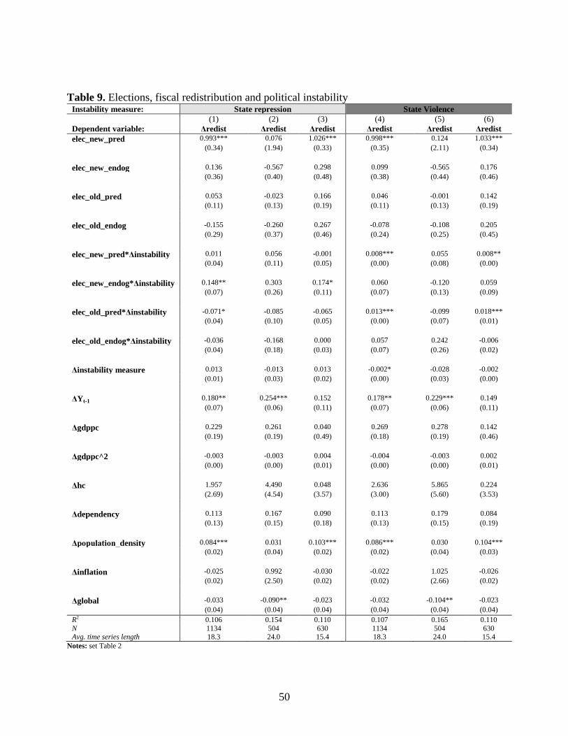
50

Table 9. Elections, fiscal redistribution and political instability Instability measure: State repression State Violence

(1) (2) (3) (4) (5) (6)

Dependent variable: Δredist Δredist Δredist Δredist Δredist Δredist elec_new_pred 0.993*** 0.076 1.026*** 0.998*** 0.124 1.033***

(0.34) (1.94) (0.33) (0.35) (2.11) (0.34)

elec_new_endog 0.136 -0.567 0.298 0.099 -0.565 0.176

(0.36) (0.40) (0.48) (0.38) (0.44) (0.46)

elec_old_pred 0.053 -0.023 0.166 0.046 -0.001 0.142

(0.11) (0.13) (0.19) (0.11) (0.13) (0.19)

elec_old_endog -0.155 -0.260 0.267 -0.078 -0.108 0.205

(0.29) (0.37) (0.46) (0.24) (0.25) (0.45)

elec_new_pred*Δinstability 0.011 0.056 -0.001 0.008*** 0.055 0.008**

(0.04) (0.11) (0.05) (0.00) (0.08) (0.00)

elec_new_endog*Δinstability 0.148** 0.303 0.174* 0.060 -0.120 0.059

(0.07) (0.26) (0.11) (0.07) (0.13) (0.09)

elec_old_pred*Δinstability -0.071* -0.085 -0.065 0.013*** -0.099 0.018***

(0.04) (0.10) (0.05) (0.00) (0.07) (0.01)

elec_old_endog*Δinstability -0.036 -0.168 0.000 0.057 0.242 -0.006

(0.04) (0.18) (0.03) (0.07) (0.26) (0.02)

Δinstability measure 0.013 -0.013 0.013 -0.002* -0.028 -0.002

(0.01) (0.03) (0.02) (0.00) (0.03) (0.00)

ΔYt-1 0.180** 0.254*** 0.152 0.178** 0.229*** 0.149

(0.07) (0.06) (0.11) (0.07) (0.06) (0.11)

Δgdppc 0.229 0.261 0.040 0.269 0.278 0.142

(0.19) (0.19) (0.49) (0.18) (0.19) (0.46)

Δgdppc^2 -0.003 -0.003 0.004 -0.004 -0.003 0.002

(0.00) (0.00) (0.01) (0.00) (0.00) (0.01)

Δhc 1.957 4.490 0.048 2.636 5.865 0.224

(2.69) (4.54) (3.57) (3.00) (5.60) (3.53)

Δdependency 0.113 0.167 0.090 0.113 0.179 0.084

(0.13) (0.15) (0.18) (0.13) (0.15) (0.19)

Δpopulation_density 0.084*** 0.031 0.103*** 0.086*** 0.030 0.104***

(0.02) (0.04) (0.02) (0.02) (0.04) (0.03)

Δinflation -0.025 0.992 -0.030 -0.022 1.025 -0.026

(0.02) (2.50) (0.02) (0.02) (2.66) (0.02)

Δglobal -0.033 -0.090** -0.023 -0.032 -0.104** -0.023

(0.04) (0.04) (0.04) (0.04) (0.04) (0.04)

R2 0.106 0.154 0.110 0.107 0.165 0.110

N 1134 504 630 1134 504 630 Avg. time series length 18.3 24.0 15.4 18.3 24.0 15.4

Notes: set Table 2