2011

Fiscal Policy, Government

Budget, Public Debt

Ing. Helena Horska, Ph.D.

Chapter 5 2

5.1 Fiscal policy – stabilization role

Fiscal policy is a macroeconomic stabilization policy, which attempts to stabilize the

economy (or eliminate output gaps). Fiscal policy is the use of government

expenditure and revenue collection (taxation) to influence the economy. The two

main instruments of fiscal policy are, thus, government expenditure and revenue

(taxation). Changes in the level and composition of taxation and government

spending can impact the following variables in the economy:

aggregate demand (AD = C + I + G + NX) and the level of economic activity;

the pattern of resource allocation;

the distribution of income.

Fiscal policy refers to the use of the government budget to influence the first of these:

economic activity.

In the text below, we focus on the use of fiscal policy to affect planned expenditure.

However, fiscal policy may affect potential output as well as planned aggregate

expenditure. On the spending side, for example, investments in public capital, such

as roads, and school, can play a major role in the growth of potential output. On the

other side, taxes and transfers may well affect the incentives and economic behavior

of firms and households.

The government budget balance can be expressed by following equation:

TA = G + TR, (5.1)

where TA is the total taxes (total governments‘ revenues), TR are transfers

(examples of certain transfer payments include welfare (financial aid), social security,

and government subsidies for certain businesses; transfers generally increase

income of households and firms), and G are government expenditure. The

government budget may be balanced: TA = G + TR or in deficit: TA < G + TR, or in

surplus when TA > G + TR. If the government intends to decrease a budget deficit, it

must increase budget revenues (by higher taxes or selling government assets) and/or

Chapter 5 3

reduce budget expenditure (e.g. social benefits, government investment or

consumption).

J.M. Keynes’s theory suggested that active government policy could be effective in

managing the economy. Rather than seeing unbalanced government budgets as

wrong, Keynes advocated what has been called countercyclical fiscal policies, that

is policies which acted against the tide of the business cycle: deficit spending when a

nation's economy suffers from recession or when recovery is long-delayed and

unemployment is persistently high - and the suppression of inflation in boom times by

either increasing taxes or cutting back government outlays. He argued that

governments should solve problems in the short run rather than waiting for market

forces to do it in the long run, because ‘in the long run, we are all dead’. This

contrasted with the classical and neoclassical economic analysis of fiscal policy.

Fiscal stimulus (deficit spending) could actuate production. But to these schools,

there was no reason to believe that this stimulation would outrun the side-effects that

’crowd out’ private investment: first, it would increase the demand for labor and raise

wages, hurting profitability; second, a government deficit increases the stock of

government bonds, reducing their market price and encouraging high interest rates,

making it more expensive for business to finance fixed investment. Thus, efforts to

stimulate the economy would be self-defeating.

The Keynesian response is that such fiscal policy is only appropriate when

unemployment is persistently high (above the non-accelerating inflation rate of

unemployment (NAIRU)1). In that case, crowding out is minimal. Further, private

investment can be ‘crowded in‘: fiscal stimulus raises the market for business output,

raising cash flow and profitability, spurring business optimism. To Keynes, this

accelerator effect means that government and business could be complements

rather than substitutes in this situation. Second, as the stimulus occurs, gross

domestic product rises, raising the amount of saving, helping to finance the increase

in fixed investment. Finally, government outlays need not always be wasteful:

government investment in public goods that will not be provided by profit-seekers will

encourage the private sector's growth. That is, government spending on such things 1

For more details see Ch 7.

Chapter 5 4

as basic research, public health, education, and infrastructure could help the long-

term growth of potential output. The conservative and some neoliberal economists

view the problem of higher unemployment from different perspective: they state that

unless labor unions or the government ‘meddle’ in the free market, persistently higher

unemployment is created. Their solution is to increase labor-market flexibility, e.g., by

cutting wages, busting unions, and deregulating business.

Contrary to some critical characterizations of it, Keynesianism does not consist solely

of deficit spending. Keynesianism recommends counter-cyclical policies to smooth

out fluctuations in the business cycle. An example of a counter-cyclical policy is

raising taxes to cool the economy and to prevent inflation when there is abundant

demand-side growth, and engaging in deficit spending on labor-intensive

infrastructure projects to stimulate employment and stabilize wages during economic

downturns. Classical economics, on the other hand, argues that one should cut taxes

when there are budget surpluses, and cut spending - or, less likely, increase taxes -

during economic downturns. Keynesian economists believe that adding to profits and

incomes during boom cycles through tax cuts, and removing income and profits from

the economy through cuts in spending and/or increased taxes during downturns,

tends to exacerbate the negative effects of the business cycle. This effect is

especially pronounced when the government controls a large fraction of the

economy, and is therefore one reason fiscal conservatives advocate a much smaller

government.

According J.M. Keynes, excessive saving, i.e. saving beyond planned investment, is

a serious problem, encouraging recession or even depression. Excessive saving

results if investment falls, perhaps due to falling consumer demand, over-investment

in earlier years, or pessimistic business expectations, and if saving does not

immediately fall in step, the economy would decline. Contrary, the classicals wanted

to balance the government budget. To Keynes, this would exacerbate the underlying

problem: following either policy would raise saving (broadly defined) and thus lower

the demand for both products and labour.

Chapter 5 5

5.2 Short-run equilibrium output – Keynesian Cross

Self-study: Franke (2007): Ch 26

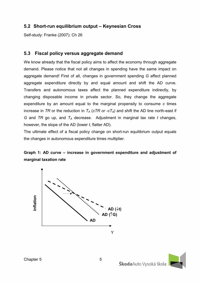
5.3 Fiscal policy versus aggregate demand

We know already that the fiscal policy aims to affect the economy through aggregate

demand. Please notice that not all changes in spending have the same impact on

aggregate demand! First of all, changes in government spending G affect planned

aggregate expenditure directly by and equal amount and shift the AD curve.

Transfers and autonomous taxes affect the planned expenditure indirectly, by

changing disposable income in private sector. So, they change the aggregate

expenditure by an amount equal to the marginal propensity to consume c times

increase in TR or the reduction in TA (cTR or -cTA) and shift the AD line north-east if

G and TR go up, and TA decrease. Adjustment in marginal tax rate t changes,

however, the slope of the AD (lower t, flatter AD).

The ultimate effect of a fiscal policy change on short-run equilibrium output equals

the changes in autonomous expenditure times multiplier.

Graph 1: AD curve – increase in government expenditure and adjustment of

marginal taxation rate

infl

ati

on

AD

AD (G)

AD (t)

Y

Chapter 5 6

If the economy falls into a recession (Y<Y*; see point A in Graph 2), the government

may decide to support the economy in order to shorten the period of recession and

low employment by reducing the marginal tax rate (t). Instead of relaying on self-

correction of the economy that would shift the economy back to the long-term

equilibrium at point E, the economy is shifted to point B. The lower effective tax rate

increased disposable income of households. A part of disposable income was spent

on consumption, which in turn increased the AD. The point B is the point of the short

term and therefore unstable equilibrium. The higher demand forces prices up and the

SRAS line moves up. Finally, the economy moves to the long-term equilibrium level

at point F. Output reaches potential at higher inflation rate. In this case, we assumed

that fiscal policy responds to the economic imbalance alone (in isolation) without

coordination with monetary policy or countercyclical monetary policy measures.

Graph 2 Recession gap

y

infla

tion

SRAS´

AD

y*

B SRASA0

1

yA

AD (t)E

F

yB

LRAS

Chapter 5 7

In contrary, if the economy moves above the potential, in expansionary gap (Y>Y*,

point M in Graph 3), than the government may raising taxes in order to reduce

government deficit (again we do not assume any response of monetary policy). The

AD curve turns southwest. Higher taxes reduce demand, producers produce less.

Inflation decelerates to ´. Finally, the economy stabilizes in the long run equilibrium

point N. The expansionary gap is eliminated, output reaches potential and inflation

decelerates.

Graph 3 Expansionary gap

Economists debate the effectiveness of fiscal stimulus. The argument mostly centers

on crowding out, a phenomenon where government borrowing leads to higher

interest rates that offset the stimulative impact of government spending. The

complete crowding out effect is illustrated in the following graph. In this example, we

assume that the government decides, even though the economy was on the potential

- at the long run equilibrium point, boosting aggregate demand by higher government

expenditure. The result is, as you can see, pure and simple increase in inflation rate.

During the adjustment process, the economy pass through the point O, where output

is above potential and inflation remains (temporarily) stable. Producers register

higher aggregate demand boosted by higher government spending and begin

gathering the relative prices. Inflation expectations gradually rise and consequently

the rate of inflation itself. Thus, the economy shifts to the point L – to the long-term

y

infla

ce

SRAS´

AD (t)

y*

M SRAS0

´

AD N

yM

LRAS

Chapter 5 8

equilibrium at higher rate of inflation. However, higher inflation and higher inflation

expectations cause the real interest rates to grow, since the central bank aims to

save price stability. Thus, the central bank raises interest rates and pushes the MP

line up, Lenders require higher nominal interest rates from borrowers including the

‘inflation premium’ that reflects higher inflation expectations. Higher real interest rates

reduce interest rate-sensitive private consumption and private investment. Fiscal

stimulus in the form of higher government spending crowds out private spending – or

it changes the structure of expenditure in favor of public expenditure. The total

expenditure (ie aggregate demand) remain unchanged. Ideally, if inflation

expectations are fully rational and the central bank’s tightening monetary policy

successfully prevents inflation advances, the economy comes back from point O to

point K. Inflation does not change, output is back on potential. The AD line is also

back at its initial position. But if inflation expectations are irrational and economic

agents underestimate an increase in inflation, the SRAS line will not move to the

point L, but somewhere between O and L and there will be a longer process of

economic adoption. The equilibrium would be achieved once the economic agents

fully adopted the final impact of initial fiscal expansion, so the economy moves to the

point L. In partial stages of economic adoption occurs so-called partial crowding-out

effect. Economic agents that do not fully adopt the final increase in inflation require a

smaller increase in interest rates and central bank (because of only moderate

increase in inflation expectations0 has to increase its key rate by less extent. As

result, the economy may stay for a while about potential but once the inflation

expectations fully reflect the true effect of fiscal expansion on inflation, the central

bank has to rise interest rate by full extent in line with its monetary policy reaction

function; the AD shifts south-west, back to the potential output at point K.

Chapter 5 9

Graph 4 Complete crowding-out effect

Summarization of the fiscal policy effects:

A) Expansive fiscal policy in the short and medium term leads to the growth of

aggregate spending and production, if we assume that expectations of

economic agents are not fully rational. If expectations are fully rational, the

point B) is correct.

B) in a sufficiently long period when economic agents fully incorporate into their

expectations the true impacts of expansionary fiscal policy, the fiscal stimulus

leads only to higher inflation and real interest rates. Higher real interest rates

have negative impact on investment and interest-rate sensitive consumption;

the output return back to potential and the structure of aggregate demand

changes in favor of government’s consumption. So, crowding out completely

negates any fiscal stimulus.

In other words, when the government runs a budget deficit, funds will need to

come from public borrowing (the issue of government bonds), overseas

borrowing, or monetizing the debt. When government finances a deficit by an

issue of government bonds, interest rates can increase across the market,

because government borrowing creates higher demand for credit in the

financial markets. This causes a lower aggregate demand for goods and

services, contrary to the objective of a fiscal stimulus.

C) In a very long-run period, an increase in real interest rates may have a

negative impact on investment, capital formation and hence the potential,

which we have not considered in the AS-AD model. However, there are two

y

infla

ce

SRAS´

AD

y*

SRAS

´

AD´ (G)

K

L

yo

OSRAS´´

LRAS

Chapter 5 10

channels to do so. First, expansionary fiscal policy increases the real interest

rate, reduces the growth of private investment, capital formation and ultimately

the growth of potential output. Second, government deficits lower national

savings in the economy, since government savings are negative. Funding

sources are decreasing and capital formation and investment decline. The

decline in capital formation may result in slower growth of potential output.

Neoclassical economists generally emphasize crowding out while Keynesians argue

that fiscal policy can still be effective especially in a liquidity trap where, they argue,

crowding out is minimal.

Shortcomings of fiscal policy

Fiscal policy is not always flexible enough to be useful for economic stabilization. In

reality, changes in government spending or taxes must usually go through a lengthy

legislative process, which reduces the ability of fiscal policy to respond in a timely

way to economic conditions. Another factor that limits the flexibility of fiscal policy is

that fiscal policymakers have many other objectives besides stabilizing aggregate

demand, from ensuring and adequate national defense to providing income support

to the poor.

Other possible problems with fiscal stimulus include the time lag between the

implementation of the policy and detectable effects in the economy, and inflationary

effects driven by increased demand. In theory, fiscal stimulus does not cause inflation

when it uses resources that would have otherwise been idle. For instance, if a fiscal

stimulus employs a worker who otherwise would have been unemployed, there is no

inflationary effect; however, if the stimulus employs a worker who otherwise would

have had a job, the stimulus is increasing labor demand while labor supply remains

fixed, leading to wage inflation and therefore price inflation.

Generally, the fiscal policy has contrary to the monetary policy one disadvantage: the

longer time lag. While the central bank’s decision - to change interest rates - is

applicable mostly the very next day after the decision, a new tax law, preparing the

state budget, all takes much longer time. Implementation lag of fiscal policy is longer

Chapter 5 11

than in the case of monetary policy. In the case of a prolonged recession or inflation,

the limited flexibility of fiscal policy recedes into the background.

Fiscal policy is implemented not only through active government interventions into

the economy that are known in the economics literature as a discretionary

government policy, but also through so-called automatic stabilizers. The

automatic stabilizers are the statutory provisions that imply automatic increases in

government spending or decrease in taxes when real output declines. When output

declines, income tax collections fall (because households’ taxable incomes fall and

subsequently consumption); contrary, the unemployment rise thus unemployment

insurance payments and welfare benefits go up – all without any explicit action by the

government or parliament. These automatic changes in government spending and

tax collections help to increase (or at least decelerate the fall in) planned spending

during recessions. During expansions, they help to reduce or slow-down the

expenditure growth, without the delays in the legislative process. The example of the

automatic stabilizer is the progressive taxation or all kinds of social benefits and

transfers.

Fiscal policy is also important stabilizing force for the cases of prolonged episodes of

recessions. However, because of the relative lack of flexibility of fiscal policy,

monetary policy is more usually applied to stabilize the economy.

Chapter 5 12

5.4 Government finance statistics

Government finance statistics (GFS) show the economic activities of government.

The GFS presentation is similar to that of business accounting where the profit and

loss accounts and the balance sheet are presented together, in a linked manner. The

emphasis is on the economic substance over the legal form of the event. Hence GFS

differ noticeably from the budget or public accounting presentations that are

nationally specific as far as scope of units and recording of transactions are

concerned. European GFS are produced in accordance with the European System of

Accounts 1995 (ESA 95), the EU manual for national accounts, supplemented by

further interpretation and guidance from Eurostat. GFS form the basis for fiscal

monitoring in Europe, most notably for the statistics related to the Excessive Deficit

Procedure (EDP).

The general government sector is divided into four sub-sectors:

a) central government (all administrative departments of the State and other central

agencies except for the administration of social security funds)

b) state government

c) local government

d) social security funds.

Total general government revenue comprises the following categories of the

European System of Accounts 1995 (ESA 95):

market output

output for own final use

payments for the other non-market output

taxes on production and imports

other subsidies on production receivable

property income

current taxes on income, wealth, etc.

social contributions

other current transfers

capital transfers

Chapter 5 13

Graph 5 General Government Revenue

Source: Eurostat, 2010.

Note: Data from 2008.

Self study: http://epp.eurostat.ec.europa.eu/cache/ITY_OFFPUB/KS-SF-10-

023/EN/KS-SF-10-023-EN.PDF

Total general government expenditure (economic types):

o intermediate consumption

o gross capital formation

o compensation of employees

o other taxes on production

o subsidies payable

o property income

o current taxes on income, wealth, etc.

o social benefits other than social transfers in kind

o social transfers in kind related to expenditure on products supplied to

households via market producers

o other current transfers

0

5

10

15

20

25

Taxes o

n

pro

duction a

nd

import

s

Curr

ent

taxes

on incom

e

Capital ta

xes

Socia

l

contr

ibutions

in %

GD

P

CR

Germany

EU27

Chapter 5 14

o adjustment for the change in net equity of households in pension fund

reserves

o capital transfers payable

o acquisitions less disposals of non-financial non-produced assets

Total general government expenditure according to function (COFOG)

Defence

Public order and safety

Economic affairs

Environment protection

Housing and community amenities

Health

Recreation; culture and religion

Education

Social protection

Graph 6 General Government Expenditure – function

Source: Eurostat, 2010.

Note: Data from 2008.

0

5

10

15

20

25

Ge

ne

ral p

ub

lic s

erv

ice

s

De

fen

ce

Pu

blic

ord

er

an

d s

afe

ty

Eco

no

mic

aff

air

s

En

vir

on

me

nt

pro

tectio

n

Ho

usin

g a

nd

co

mm

un

ity

am

en

itie

s

He

alth

Re

cre

atio

n;

cu

ltu

re a

nd

re

ligio

n

Ed

uca

tio

n

So

cia

l p

rote

ctio

n

in %

GD

P

CR

Germany

EU27

Chapter 5 15

Self-study: Eurostat (2011). EU27 and euro area government expenditure-to-GDP

ratios falling after 10 quarters of growth - Issue number 13/2011.

http://epp.eurostat.ec.europa.eu/cache/ITY_OFFPUB/KS-SF-11-013/EN/KS-SF-11-

013-EN.PDF

Graph 7 Government Budget Balance EU-25

Source: Eurostat, 2010.

5.4.2 Tax burden

For international comparison of tax burden we may use a so-called tax quota. This is

a macroeconomic indicator that is calculated as “proportion of tax and duty revenue

to GDP” in current prices (tax quota in % = tax revenues / GDP * 100). It represents a

proportion of gross domestic product that is redistributed by means of public budgets.

As it uses data of really collected tax revenues to GDP, it provides information about

-15

-13

-11

-9

-7

-5

-3

-1

1

3

5

Sw

ede

n

Lu

xem

brE

sto

nia

Fin

lan

dD

en

ma

rk

Ger

ma

nA

ustr

iaM

alta

Bu

lgar

iaH

un

ga

ryIt

aly

Net

he

rla

Slo

ven

iaC

RB

elg

ium

Cyp

rus

EU

-27

Slo

vakia

Pol

an

d

Fra

nce

Ru

ma

nia

Lith

uan

ia

La

tvia

Po

rtug

al

Sp

ain

VB

Gre

ece

Irel

an

d

in %

GD

P

2008

2009

Chapter 5 16

value of total effective taxation in the given country. Depending on the ’extent’ of

numerator (i.e. “extent” of public revenues considered), there is a simple and a

compound (sometimes called overall) tax quota. Simple tax quota includes only

those incomes of public budgets that are really labelled as taxes. With regard to the

fact that tax revenue (quasi taxes) are in fact also incomes from the obligatory

payments to social welfare, contributions to state unemployment policy and obligatory

payments to health insurance system, the relevant indicator for international

comparison is the compound tax quota that also includes these incomes. Compound

tax quota (CTQ) is calculated as proportion of revenue from tax, duty and payments

to health insurance and social welfare systems to GDP in current prices (Compound

tax quota in % = tax revenues + quasi taxes / GDP * 100). As it results from the

formula, basic factors affecting value of tax quota is the amount of gross domestic

product and volume of taxes collected. Total effective burden is regularly monitored

by Eurostat and published in the form of tax quota.

Graph 8 Compound tax quota in Europe

Source: Eurostat (2002). Main national accounts tax aggregates.

0

10

20

30

40

50

60

70

80

90

Rom

ania

Slo

vakia

Latv

ia

Lithuania

Ire

land

Est

onia

Bulg

aria

Spain

Pola

nd

Gre

ece

CR

Luxem

bu

rg

Port

ugal

Slo

venia

VB

Cyp

rus

Neth

erlan

ds

Hungary

EU

-27

Germ

an

y

EM

U (

16)

Italy

Fin

land

Aust

ria

Fra

nce

Belg

ium

Sw

ed

en

Den

mark

Malta

in %

GD

P

2007

2008

Chapter 5 17

The Laffer curve is a theoretical representation of the relationship between

government revenue raised by taxation and all possible rates of taxation. It is used to

illustrate the concept of taxable income elasticity (that taxable income will change in

response to changes in the rate of taxation). The curve is constructed by thought

experiment. First, the amount of tax revenue raised at the extreme tax rates of 0%

and 100% is considered. It is clear that a 0% tax rate raises no revenue, but the

Laffer curve hypothesis is that a 100% tax rate will also generate no revenue

because at such a rate there is no longer any incentive for a rational taxpayer to earn

any income, thus the revenue raised will be 100% of nothing. If both a 0% rate and

100% rate of taxation generate no revenue, it follows that there must exist at least

one rate in between where tax revenue would be at a maximum. However, there are

infinitely many curves satisfying these boundary conditions. Little can be said without

further assumptions or empirical data.

One potential result of the Laffer curve is that increasing tax rates beyond a certain

point will become counterproductive for raising further tax revenue because of

diminishing returns. A hypothetical Laffer curve for any given economy can only be

estimated and such estimates are sometimes controversial. Estimates of revenue-

maximizing tax rates have varied widely with some studies suggesting midpoint

ranges around 70%.

A. Laffer explains the model in terms of two interacting effects of taxation: an

’arithmetic effect’ and an ’economic effect’. The ’arithmetic effect’ assumes that tax

revenue raised is the tax rate multiplied by the revenue available for taxation (or tax

base). At a 0% tax rate, the model assumes that no tax revenue is raised. The

’economic effect’ assumes that the tax rate will have an impact on the tax base itself.

At the extreme of a 100% tax rate, the government theoretically collects zero revenue

because taxpayers change their behavior in response to the tax rate: either they

have no incentive to work or they find a way to avoid paying taxes. Thus, the

’economic effect’ of a 100% tax rate is to decrease the tax base to zero. If this is the

case, then somewhere between 0% and 100% lies a tax rate that will maximize

revenue.

Chapter 5 18

The relationship between tax rate and tax revenue is likely to vary from one economy

to another and depends on the elasticity of supply for labor and various other factors.

Even in the same economy, the characteristics of the curve could vary over time.

Complexities such as possible differences in the incentive to work for different

income groups and progressive taxation complicate the task of estimation. The

structure of the curve may also be changed by policy decisions. For example, if tax

loopholes and off-shore tax shelters are made more readily available by legislation,

the point at which revenue begins to decrease with increased taxation is likely to

become lower.

A. Laffer presented the curve as a pedagogical device to show that, in some

circumstances, a reduction in tax rates will actually increase government revenue

and not need to be offset by decreased government spending or increased

borrowing. For a reduction in tax rates to increase revenue, the current tax rate would

need to be higher than the revenue maximizing rate. In 2007, Laffer said that the

curve should not be the sole basis for raising or lowering taxes.

Graph 9 Laffer curve

Tax rate „t“t*0 100 %

Tax

reve

nues

Chapter 5 19

5.4.3 General government budget

Primary balance

Primary balance is the general government balance which is derived after deducting

the interest payments component from the total balance of general government

budget. In other words, the total of primary deficit and interest payments makes the

general government deficit.

A government deficit can be measured with or without including the interest it pays on

its debt. The primary deficit is defined as the difference between current

government spending and total current revenue from all types of taxes. The total

deficit (which is often just called the 'deficit') is spending, plus interest payments on

the debt, minus tax revenues.

Therefore, if Gt is government spending and Tt is tax revenue for the respective

timeframe, then the primary deficit is

Gt - Tt.

If Bt − 1 is last year's debt, and i is the interest rate, then the total deficit is

Dt = Gt + iBt−1 - Tt. (5.2)

Graph 10 General Government Balance in the Czech Republic

Source: Ministry of Finance of the Czech Republic (2001). Macroeconomic Forecast. July 2010, GFS

2001 Statistics.

-8

-7

-6

-5

-4

-3

-2

-1

0

1

2004 2005 2006 2007 2008 2009

in %

GD

P

General Government Balance

Primary balance

Chapter 5 20

Structural deficit

A government deficit can be thought of as consisting of two elements, structural and

cyclical. At the lowest point in the business cycle, there is a high level of

unemployment. This means that tax revenue are low and expenditure (e.g. on social

security) high. Conversely, at the peak of the cycle, unemployment is low, increasing

tax revenue and decreasing social security spending. The additional borrowing

required at the low point of the cycle is the cyclical deficit. By definition, the cyclical

deficit will be entirely repaid by a cyclical surplus at the peak of the cycle.

The structural deficit is the deficit that remains across the business cycle, because

the general level of government spending is too high for prevailing tax levels. The

observed total budget deficit is equal to the sum of the structural deficit with the

cyclical deficit or surplus.

Structural deficit differs from cyclical deficit in that it exists even when the economy is

at its potential. Structural deficit issues can only be addressed by explicit and direct

government policies: reducing spending (including social benefits), increasing the tax

base, and/or increasing tax rates.

The fiscal gap, a measure proposed by economists Alan Auerbach and Laurence

Kotlikoff, measures the difference between government spending and revenues over

the very long term, typically as a percentage of Gross Domestic Product. The fiscal

gap can be interpreted as the percentage increase in revenues or reduction of

expenditures necessary to balance spending and revenues in the long run. For

example, a fiscal gap of 5% could be eliminated by an immediate and permanent 5%

increase in taxes or cut in spending or some combination of both. It includes not only

the structural deficit at a given point in time, but also the difference between promised

future government commitments, such as health and retirement spending, and

planned future tax revenues. Since the elderly population is growing much faster than

the young population in many countries, many economists argue that these countries

have important fiscal gaps, beyond what can be seen from their deficits alone.

Chapter 5 21

Stances of fiscal policy

There are three possible stances of fiscal policy: neutral, expansionary and

contractionary. The simplest definitions of these stances are as follows:

A neutral stance of fiscal policy implies a balanced economy. Government

spending is fully funded by tax revenue and overall the budget outcome has a

neutral effect on the level of economic activity.

An expansionary stance of fiscal policy involves government spending

exceeding tax revenue; the budget outcome supports the economic activity.

A contractionary fiscal policy occurs when government spending is lower than

tax revenue; the budget outcome has a negative impact on the economic

activity.

However, these definitions can be misleading because, even with no changes in

spending or tax laws at all, cyclical fluctuations of the economy cause cyclical

fluctuations of tax revenue and of some types of government spending, altering the

deficit situation; these are not considered to be policy changes. Therefore, for

purposes of the above definitions, ’government spending‘ and ’tax revenue‘ are

normally replaced by ’cyclically adjusted government spending‘ and ’cyclically

adjusted tax revenue‘. Thus, for example, a government budget that is balanced over

the course of the business cycle is considered to represent a neutral fiscal policy

stance. So, to evaluate the fiscal policy stance is better to use the structural balance.

If the structural deficit increases or structural surplus is reduced, the fiscal stance is

expansionary; if the structural deficit decreases or the structural surplus raises, the

fiscal policy is contractionary. Changes in the structural government balance are

sometimes defined as the fiscal position. And the fiscal position measures whether

the government sector adds funds into the economy or removes them.

Chapter 5 22

5.5 Public Debt

5.5.1 Methods of funding government deficit

Governments spend money on a wide variety of things, from the military and police to

services like education and healthcare, as well as transfer payments such as welfare

benefits. This expenditure can be funded in a number of different ways:

Taxation

Seigniorage (the benefit from printing money)

Borrowing money from the population or from abroad

Consumption of fiscal reserves

Sale of fixed assets (e.g. land; state-own companies)

All of these except taxation, seigniorage and a reduction of government expenditures

are forms of debt financing.

Seigniorage is the main profit of the central bank and as public institution, the central

bank is required to pass most of their profits to their government. So, it is profit of the

government. Formally, seigniorage is the real value of the monetary base created. Or

it is the difference between interest earned on securities acquired in exchange for

bank notes and the costs of producing and distributing those notes. To put more

simple, the seigniorage is a profit from ‘printing’ money.

Some economists regarded seigniorage as a form of inflation tax, redistributing real

resources to the currency issuer. Issuing new currency, rather than collecting taxes

paid out of the existing money stock, is then considered in effect a tax that falls on

those who hold the existing currency. The expansion of the money supply may cause

inflation in the long run.

Monetization of the public debt describes the situation when the government

borrows from commercial banks by issuing Treasury bills which are then acquired by

the central bank on the open market. The direct lending to the government through

the credit or direct purchase of Treasury bill by the central bank is in the most of the

Chapter 5 23

developed economies forbidden. Most of the episodes of high inflation are associated

with direct financing of budget deficits and/or monetization of the debt.

Borrowing

A fiscal deficit is often funded by issuing bonds, like Treasury bills. These pay

interest, either for a fixed period or indefinitely. If the interest and capital repayments

are too large, a nation may default on its debts, usually to foreign creditors.

A fiscal surplus is often saved for future use, and may be invested in local (same

currency) financial instruments, until needed. When income from taxation or other

sources falls, as during an economic slump, reserves allow spending to continue at

the same rate, without incurring additional debt.

Government debt can be categorized as internal debt, owed to lenders within the

country (residents), and external debt, owed to foreign lenders. Bonds issued by

national governments in foreign currencies are normally referred to as sovereign

bonds.

And what is the impact of debt financing of the deficit in the economy? To answer the

equation, we can use the identity of savings and investment in a closed economy:

S = I (5.3)

National savings S and planned investment can be divided into private and

government:

SG + SP = IG + IP.

If the government runs budget deficits, the government savings are negative. This

means that the government has to draw private funds - private savings. The possible

short-fall of private savings in the economy causes interest rate to rise. And private

investment is to decline (see crowding-out) and so the potential in long run.

In the case of an open economy, the goverment deficit could be financed by foreign

economic agents. The possible lack of savings in the domestic economy would be

Chapter 5 24

reflected in the current account deficit (correspondingly in a surplus in financial

account within balance of payment):

S - I = BU. (5.4)

Government deficit might be covered partially or entirely from foreign sources. And if

capital mobility is perfect over the globe, domestic real interest rate should be equal

to foreign interest rates. In this case, no crowding out of the private investment will

occur.

5.5.2 The Arithmetic of Deficits and Debt

Public debt is incurred by the accumulation of government deficits. So, the actual

level of public debt can be calculated as the sum of the debt in year t-1 (Bt-1) and the

actual government deficit in year t Dt:

Bt = Bt-1 + Dt. (5.5)

The government budget constraint states that the change in government debt

during year t is equal to the deficit during year t

Bt - Bt-1 = Dt. (5.6)

Further, we assume that the government deficit is equal to sum of interest rate

payments on the government debt (iBt-1), government expenditures (Gt) and transfers

(TRt) reduced by government tax revenue (TAt).

Dt = iBt-1 + Gt + TRt - TAt. (5.7)

From last two equation is clear that if the government runs a deficit, than the

government debt increases. If the government runs a surplus, government debt

decreases.

Using the above definition of the deficit, we can rewrite the government budget

constraint as

Bt - Bt-1 = iBt-1 + Gt + TRt - TAt, (5.8)

Chapter 5 25

where iBt-1 are (nominal) interest payments on the debt, (Gt + TRt - TAt) is the primary

deficit (equivalently, primary surplus would be TAt -Gt - TRt).

Reorganizing the government budget constraint by shifting Bt-1 on the right side of

the equation, we get:

Bt = (1+i)Bt-1 + Gt + TRt - TAt. (5.9)

Now we look at the implications.

A) Eliminating primary deficit and making primary balance balanced

Suppose that the government decides to eliminate primary deficit. The cumulated

debt would increase further, at the rate equal to (1+i):

Bt = (1+i)Bt-1 + 0.

So the debt would keep increasing over time. The reason is clear: while the primary

deficit is equal to zero, debt was and still is positive, and so are interest payments on

the debt. Each year the government must issue more debt to pay the interest on

existing debt.

B) Debt stabilization

Suppose that the government decides to stabilize the debt on the level of Bt-1. So, the

actual debt Bt must equal to previous one Bt-1:

0 = Bt - Bt-1 = iBt-1 + Gt + TRt - TAt.

Reorganizing, we get:

iBt-1 = TAt - Gt - TRt.

To avoid a further increase in debt, the government must run a primary surplus equal

to interest rate payments on the existing debt. And it must do so in following years as

well: each year, the primary surplus must be sufficient to cover interest payments,

keeping the debt level unchanged.

C) Full repayment

Suppose the government decides to fully repay the debt. So Bt = 0:

0 = (1+i)Bt-1 + Gt + TRt - TAt.

Chapter 5 26

Even with the balanced primary deficit, the government debt is increasing at the rate

equal to the interest rate:

Bt=(1+i)t-1 and Bt+1=(1+i)t, and Bt+2=(1+i)t+1,…

or to go back to the past:

Bt=(1+i)t-1 and Bt-1=(1+i)t-2, and Bt-2=(1+i)t-3,…

Now, back to the government budget constraint, where we substitute Bt-1 by (1+i)t-2:

0 = (1+i)(1+i)t-2+ Gt + TRt - TAt.

0 = (1+i)t-1+ Gt + TRt - TAt.

Reorganizing the above equation we get:

(1+i)t-1 = TAt - Gt - TRt .

This expression states that the government must run primary surplus equal to (1+i)t-1

(interest payment in t-1 year) to full repay the debt.

These examples yields the below set of conclusions:

o The legacy of past deficits is higher government debt.

o To stabilize the debt, the government must eliminate the deficit

o To eliminate the deficit, the government must run a primary surplus equal

to the interest payments on the existing debt.

o If the government runs into a deeper deficit, higher government spending

must eventually be off-set by an increase in taxes in the future

o The longer government waits to eliminate the deficit, the higher eventual

increase in taxes or/and decrease in spending.

The Evolution of the Debt-to-GDP ratio and the Arithmetic of the Debt Ratio

So far we have focused on the evolution of debt level. But in an economy in which

output grows over time, it makes more sense to focus instead of the ratio of debt to

output.

First, we divide both sides of the government budget constraint by actual nominal

output:

Chapter 5 27

.1)1(

tY

tTA

tTR

tG

Yt

Bi

tY

tB

t

Next we multiply Bt-1 / Yt (both the numerator and denominator) by Yt-1:

The ratio Yt-1/Yt is only the reverse ratio of Yt /Yt-1, that express the increase in output.

The annual increase in output is, however, precisely calculated as (Yt - Yt-1)/Yt-1. And

if we denote the annual rate of output by g, than Yt /Yt-1 = 1+g or Yt-1/Yt = 1/(1+g).

And we substitute Yt-1/Yt by 1/(1+g).

And using the approximation (1+i)/(1+g) = 1+i-g, we rewrite the preceding equation

as

(5.10)

The final relation has a simple interpretation. The change in the debt ratio over time

(the left side of the equation) is equal to the sum of the gap between nominal interest

rate and nominal GDP growth rate time the initial debt ratio, and the ratio of the

primary deficit to GDP. If the primary deficit is zero, debt will then increase at a rate

equal to nominal interest rate minus the growth rate of nominal output (i-g). So, if the

rate of nominal GDP exceeds the nominal interest rates and the government runs

deficit, the debt will expanded by slower pace. But if the nominal interest rates are

higher than the rate of nominal GDP growth, the debt will accelerate. The excessive

debt-to-GDP ratio or its out-off-control growth might cause the debt crisis. Once the

economic agents lose their believe that the government will fully repay the debt,

these fears can easily become self-fulfilling. The lenders will ask higher interest rate

,)1(1

11

tY

tTA

tTR

tG

Y

B

Y

Yi

tY

tB

t

t

t

t

.1

1)1(

1

1

tY

tTA

tTR

tG

Y

B

gi

tY

tB

t

t

.)(1

1

1

1

tY

tTA

tTR

tG

Y

Bgi

Y

B

tY

tB

t

t

t

t

Chapter 5 28

Primary balance in

% GDP

2008 2009e 2009e

EMU 69,4 78,7 -3,5

Germany 66 73,2 -0,7

CR 30 35,4 -4,6

Greece 95,7 99,2 -8,5

Govern. debt

in % GDP

on government debt and it might happen that the government will be unable to repay

the debt, validating initial fears.

So, there is the caution rule that says that if interest rates in an economy exceed

the growth rate of the nominal GDP and the government budget revenue, the

primary balance should turn into surplus in order not to jeopardize the long-

term stability of public budgets.

Table 1 Government debt and Primary balance

Source: Eurostat (2010). European Economic Forecast. Spring 2010.

Graph 11 Government debt to GDP

Source: Eurostat, Aug 2010.

0

20

40

60

80

100

120

Esto

nia

Luxem

bru

g

Bulg

aria

Rom

ania

Lithuania

CR

Slo

vakia

Slo

venia

Latv

ia

Denm

ark

Sw

eden

Fin

land

Pola

nd

Spain

Cypru

s

Neth

erlands

Irla

nd

Austr

ia

Gre

at

Brita

in

Malta

Germ

any

EU

-27

Port

ugal

Fra

ncie

Hungary

EM

U-1

6

Belg

ium

Gre

ece

Italy

in %

GD

P

2009

2005

Chapter 5 29

5.6 Ricardian equivalence

The Ricardian equivalence hypothesis, named after the English political economist

and Member of Parliament David Ricardo, states that because households anticipate

that current public deficit will be paid through future taxes, those households will

accumulate savings now to offset those future taxes. If households acted in this way,

a government would not be able to use tax cuts to stimulate the economy. The

Ricardian equivalence result requires several assumptions. These include

households acting as if they were infinite-lived dynasties as well as assumptions of

no uncertainty and no liquidity constraints. Also, for Ricardian equivalence to apply,

the deficit spending would have to be permanent. In contrast, a one-time stimulus

through deficit spending would suggest a lesser tax burden annually than the one-

time deficit expenditure. Thus temporary deficit spending is still expansionary.

Empirical evidence on Ricardian equivalence effects has been mixed. Insofar as

future tax increases appear more distant and their timing more uncertain, consumers

Box 1 European sovereign debt crisis (2010–present)

In early 2010, fears of a sovereign debt crisis, the 2010 Euro Crisis, developed

concerning some European states, including European Union members Portugal,

Ireland, Italy, Greece, Spain, and Belgium. This led to a crisis of confidence as well

as the widening of bond yield spreads and risk insurance on credit default swaps

between these countries and other EU members, most importantly Germany.

Concern about rising government deficits and debt levels across the globe together

with a wave of downgrading of European government debt created alarm in

financial markets. In 2010 the debt crisis was mostly centred on events in Greece,

where there was concern about the rising cost of financing government debt. On 2

May 2010, the Eurozone countries and the International Monetary Fund agreed to a

€110 billion loan for Greece, conditional on the implementation of harsh Greek

austerity measures. On 9 May 2010, Europe's Finance Ministers approved a

comprehensive rescue package worth almost a trillion dollars aimed at ensuring

financial stability across Europe by creating the European Financial Stability

Facility.

Chapter 5 30

are in fact more likely to ignore them. This may be the case because they expect to

die before taxes go up, more likely, because they just do not think that far into the

future. In either case, Ricardian equivalence is likely to fail.

So, we can conclude that budget deficits have an important effect on activity –

although perhaps a smaller effect than we though going through the Ricardian

equivalence argument. In the short-run, larger deficits are likely to lead to higher

demand and to higher output. In the long run, higher government debt lowers capital

accumulation and, as a result, lowers output, and possibly potential.

5.7 Fiscal reforms

Self-study: GUICHARD, S. at el. (2007). What promotes fiscal consolidation OECD

Country experiences. Economic Department OECD, ECO/WKP(2007)13. May 28,

2007.

5.7.2 Fiscal Straitjacket - fiscal rules

The concept of a fiscal straitjacket is a general economic principle that suggests strict

constraints on government spending and public sector borrowing, to limit or regulate

the budget deficit over a time period. The term probably originated from the definition

of straitjacket: anything that severely confines, constricts, or hinders. Various states

in the United States have various forms of self-imposed fiscal straitjackets.

Chapter 5 31

Box 2 Fiscal Rules in Europe: The Stability and Growth Pact

The Stability and Growth Pact (SGP) is an agreement among the 17 members of the

European Union (EU) that take part in the Eurozone, to facilitate and maintain the

stability of the Economic and Monetary Union. It consists of fiscal monitoring of

members by the European Commission and the Council of Ministers and, after multiple

warnings, sanctions against offending members. The pact was adopted in 1997, so that

fiscal discipline would be maintained and enforced in the EMU. Member states adopting

the euro have to meet the Maastricht convergence criteria, and the SGP ensures that

they continue to observe them. The actual criteria that member states must respect:

* an annual budget deficit no higher than 3% of GDP (this includes the sum of all

public budgets, including municipalities, regions, etc)

* a national debt lower than 60% of GDP or approaching that value.

The SGP was initially proposed by German finance minister Theo Waigel in the mid

1990s. Germany had long maintained a low-inflation policy, which had been an

important part of the German strong economy's performance since the 1950s; the

German government hoped to ensure the continuation of that policy through the SGP

which would limit the ability of governments to exert inflationary pressures on the

European economy.

Unfortunately, the pact has proved not to be enforceable against big countries such as

France and Germany, which were the biggest promoters of it when it was created.

These countries have run ’excessive’ deficits under the pact definition for some years.

The reasons that larger countries have not been punished include their influence and

large number of votes on the Council of Ministers, which must approve sanctions; their

greater resistance to ’naming and shaming’ tactics, since their electorates tend to be

less concerned by their perceptions in the European Union; their comparatively weak

commitment to the euro as compared to smaller states; the relatively greater role of

government spending in their larger and more enclosed economies.

In March 2005, the EU Council, under the pressure of France and Germany, relaxed the

rules; the EC said it was to respond to criticisms of insufficient flexibility and to make the

pact more enforceable. The Ecofin agreed on a reform of the SGP. The ceilings of 3%

for budget deficit and 60% for public debt were maintained, but the decision to declare a

country in excessive deficit can now rely on certain parameters: the behaviour of the

cyclically adjusted budget, the level of debt, the duration of the slow growth period and

the possibility that the deficit is related to productivity-enhancing procedures.

Chapter 5 32

5.8 Exercises

1. Describe and depict in the AS-AD model the stabilization process of an economy

in the case of (a) recession, and (b) the high inflation rate, if the government decides

to withdraw (or to introduce) a poll-tax in order to support the self-correction process

of the economy.

2. Using AD-AS model, describe the way how the automatic stabilizers work, namely

the unemployment benefits, if (a) the economy is hit by recession or (b) it ends up in

expansionary gaps.

3. The government decided to reduce the marginal income tax rate from 40% to 30%.

To prevent a worsening of the government budget balance, it reduces, at the same

time, the welfare benefits by 100 to 200 units. How and how much the aggregate

demand is going to be effected, if the propensity to consume c is equal to 0.8?

Assume the initial level of product 2000.

4. The government runs deficits for many years. Its debt has climbed to 500 and

debt-to-GDP ratio reached 60%. Nominal interest rates are 5% on average and the

nominal GDP is growing at 8% per annum. How high primary surplus must be in

order to stabilize the government debt (in other words, to eliminate an increase in

debt at time t to zero).

5. Use the data from Example 4 and calculate how high primary surplus of the

government must be in order to fully repay the actual debt.

Chapter 5 33

Assigned reading

FRANK, R.H. – BERNANKE, B.S. (2009) Principles of Economics. Chapter 23

p. 651-671, Appendix A&B p. 667-673. and Chapter 26 p.760-767. Fourth

Edition. USA: McGraw-Hill, 2009. 836 s. ISBN 978-0-07-128542-1.

GUICHARD, S. at el. (2007). What promotes fiscal consolidation OECD

Country experiences. Economic Department OECD, ECO/WKP(2007)13. May

28, 2007.

Self-study

BLANCHARD, O. (2002). Macroeconomics. 5th edition, Prentice-Hall 2002, Ch

26. ISBN 0-13-110301-6.

Eurostat (2011). EU27 and euro area government expenditure-to-GDP ratios

falling after 10 quarters of growth - Issue number 13/2011.

http://epp.eurostat.ec.europa.eu/cache/ITY_OFFPUB/KS-SF-11-013/EN/KS-

SF-11-013-EN.PDF.

Eurostat (2010). Tax revenue in the European Union - Issue number 23/2010.

http://epp.eurostat.ec.europa.eu/cache/ITY_OFFPUB/KS-SF-10-023/EN/KS-

SF-10-023-EN.PDF.

Sources

HORSKA H., www.horska.com

FRANK, R.H. – BERNANKE, B.S. (2009) Principles of Economics. Fourth

Edition. USA: McGraw-Hill, 2009. 836 s. ISBN 978-0-07-128542-1.

BLANCHARD, O. (2002). Macroeconomics. 5th edition, Prentice-Hall 2002,

Ch.26. ISBN 0-13-110301-6.

BURDA, M. – WYPLOSZ, Ch. (2001) Macroeconomics – A European Text. 3th

edition. Oxford University Press, 2001. Ch. 15. ISBN 0-19-877-650-0.

Czech National Bank. Inflation Report. Different issue.

Eurostat (2006). Small decline in overall taxation to 39.3% of GDP in 2004,

News Release, 62/2006, 17 May 2006.

Chapter 5 34

http://epp.eurostat.ec.europa.eu/portal/page?_pageid=1090,30070682,1090_3

3076576&_dad=portal&_schema=PORTAL.

GUICHARD, S. at el. (2007). What promotes fiscal consolidation OECD

Country experiences. Economic Department OECD, ECO/WKP(2007)13. May

28, 2007.

Ministry of Finance of the Czech Republic. Fiscal outlook of the Czech

Republic. Different issues.

Ministry of Finance of the Czech Republic. Macroeconomic forecast of the

Czech Republic. Different issues.

© Helena Horská, 2011