fiscal policies, inequality, and poverty in croatia

Radni materijali EIZ-a EIZ Working Papers

.

ekonomskiinstitut,zagreb

Listopad October. 0212

Nga Thi Viet Nguyen and Ivica Rubil

Br No. EIZ-WP-2104

Fiscal Policies,Inequality, andPoverty in Croatia

Radni materijali EIZ-a EIZ Working Papers

EIZ-WP-2104

Fiscal Policies, Inequality, and Poverty in Croatia

Nga Thi Viet Nguyen The World Bank

e-mail: [email protected]

Ivica Rubil The Institute of Economics, Zagreb

e-mail: [email protected]

www.eizg.hr

Zagreb, October 2021

IZDAVAČ / PUBLISHER: Ekonomski institut, Zagreb / The Institute of Economics, Zagreb Trg J. F. Kennedyja 7 10 000 Zagreb Hrvatska / Croatia T. +385 1 2362 200 F. +385 1 2335 165 E. [email protected] www.eizg.hr ZA IZDAVAČA / FOR THE PUBLISHER: Tajana Barbić, ravnateljica / director GLAVNA UREDNICA / EDITOR: Ivana Rašić UREDNIŠTVO / EDITORIAL BOARD: Ivan-Damir Anić Tajana Barbić Goran Buturac Antonija Čuvalo Ivica Rubil Sunčana Slijepčević Paul Stubbs Maruška Vizek e-ISSN 1847-7844 Stavovi izraženi u radovima u ovoj seriji publikacija stavovi su autora i nužno ne odražavaju stavove Ekonomskog instituta, Zagreb. Radovi se objavljuju s ciljem poticanja rasprave i kritičkih komentara kojima će se unaprijediti buduće verzije rada. Autor(i) u potpunosti zadržavaju autorska prava nad člancima objavljenim u ovoj seriji publikacija. Views expressed in this Series are those of the author(s) and do not necessarily represent those of the Institute of Economics, Zagreb. Working Papers describe research in progress by the author(s) and are published in order to induce discussion and critical comments. Copyrights retained by the author(s).

Contents

Abstract 1

1 Introduction 3

2 The Fiscal System in Croatia 5

2.1 Revenue 5

2.2 Social Spending 8

3 Methodology 10

4 Data and the Empirical Strategy for the Analysis 12

4.1 Household Survey Data 12

4.2 Fiscal Instruments 13

4.3 Empirical Strategies and Assumptions 13

4.4 Macro Validation 16

4.5 Caveats 16

5 Results: Distributional Impact of the Fiscal System in Croatia 16

5.1 Impacts on Inequality 16

5.2 Impacts on Poverty 19

6 Incidence, Progressivity, and Marginal Contributions of Taxes and Social Spending 20

6.1 Distributional Profile of the Fiscal System 20

6.2 Direct Taxes, Indirect Taxes, and Social Insurance Contributions 22

6.3 Direct and In-kind Transfers 25

7 Distributional Impacts of Tax and Social Spending Reforms, 2018 to 2021 29

7.1 Simulation Approach and Recent Reforms 29

7.2 Distributive Impact of Reforms 30

8 Conclusions and Policy Insights 35

References 37

Annex A. Description of fiscal instruments included in analysis 39

Annex B. Distributive impact of fiscal instruments included in analysis: results for scenario pensions-as-government-transfers

56

Annex C. Survey-to-survey imputation of indirect taxes 57

Annex D. Impacts of fiscal interventions on poverty 60

Annex E. Macro-validation of fiscal instruments included in analysis 62

1

Fiscal Policies, Inequality, and Poverty in Croatia

Nga Thi Viet Nguyen The World Bank

[email protected]

Ivica Rubil The Institute of Economics, Zagreb

[email protected]

Abstract In a fiscally expansionary context, policy makers in Croatia must keep in mind the redistributive role of fiscal policies, particularly their impact on inequality and poverty. This paper uses both household survey data and national accounts to estimate how in 2018 the Croatian fiscal system affected income distribution and poverty. Moreover, it assesses the individual and the combined effects of interventions like direct and indirect taxes and social spending. The analysis found that in 2018 the fiscal system helped to reduce inequality but also increased poverty. All fiscal interventions except indirect taxes (VAT and excises) reduced inequality. However, indirect taxes not only widened the income gap between rich and poor but also increased poverty—only direct transfers had poverty-reducing effects. Direct taxes (personal income tax [PIT] and property taxes) had no impact on poverty in 2018. A series of reforms introduced between 2018 and 2021 helped reduce poverty slightly, mainly because the VAT on some food items was lowered. However, these reforms pushed up inequality, mostly because PIT reforms reduced the tax burden for those with high incomes. JEL classification: H22, I38, D31 Keywords: fiscal policy, fiscal incidence, social spending, inequality, poverty, taxes, Croatia

Acknowledgements: The authors benefitted from a rich series of comments from Alan Fuchs and Josip Funda. We are grateful for valuable insight and discussion from Gabriela Inchauste, Reena Badiani-Magnusson, Jia Gao, Karolina Goraus, and Juan Pablo Baquero Vargas.

2

Fiskalna politika, nejednakosti i siromaštvo u Hrvatskoj

Sažetak U kontekstu fiskalne ekspanzije, donositelji politika u Hrvatskoj moraju imati na umu preraspodjelnu ulogu fiskalne politike, posebno njezin utjecaj na nejednakosti i siromaštvo. Ovaj rad koristi podatke iz ankete kućanstava i iz nacionalnih računa za procjenu učinka fiskalnog sustava na raspodjelu dohotka i siromaštvo u Hrvatskoj 2018. godine. Također se procjenjuje pojedinačni i kombinirani utjecaj intervencija kao što su izravni i neizravni porezi te socijalni izdaci. Analiza pokazuje da je 2018. fiskalni sustav pomogao u smanjenju nejednakosti, ali također i povećanju siromaštva. Sve fiskalne intervencije osim neizravnih poreza (PDV i trošarine) smanjivale su nejednakosti. Međutim, neizravni porezi ne samo da su proširivali jaz između bogatih i siromašnih, nego su i povećavali siromaštvo. Samo su izravni transferi smanjivali siromaštvo. Izravni porezi (porez na dohodak i porezi na imovinu) nisu utjecali na siromaštvo u 2018. Niz reformi u razdoblju od 2018. do 2021. pomogle su blagom smanjenju siromaštva, uglavnom zbog sniženja PDV-a na određene prehrambene artikle. Međutim, te su reforme povećale nejednakosti, uglavnom zbog toga što su reforme poreza na dohodak smanjile porezni teret za one s visokim dohocima. JEL klasifikacija: H22, I38, D31 Ključne riječi: fiskalna politika, fiskalna incidenca, socijani izdaci, nejednakosti, siromaštvo, porezi, Hrvatska

3

1 Introduction Over the past decade, fiscal policy in Croatia can be classified as two distinct periods: fiscal consolidation between 2009 and 2017, and fiscal expansion since 2018. Both have had significant implications for poverty and inequality. Determined consolidation efforts in the first period were reinforced in 2014 when Croatia entered the European Union (EU) Excessive Deficit Procedure that required consolidation measures on both the revenue and expenditure sides of the budget. Between 2014 and 2017 the share of the Croatian population living on less than $5.50 a day, revised 2011 purchasing power parity (PPP), dropped from 5.8 to 3.6 percent, after a period starting with the 2009 global crisis when poverty went up. The second period started with comprehensive tax reform designed to reduce the overall tax burden. In both periods, spending on health and education increased. In 2018 poverty fell further, to 2.4 percent, and is estimated to have gone down in 2019 by 2.2 percent. The trend for inequality is similar.1

But the relationship between the fiscal system and citizen welfare is complex. Often interactions between individual policies can alter the compounded impact of a fiscal package on poverty and inequality. Understanding the role of each policy—e.g., direct and indirect taxes, social insurance contributions, cash transfers, and in-kind transfers—and their combined effect in reducing poverty and redistributing income is crucial to reforming fiscal policy. That is the objective of this paper.

Here, we use standard incidence analysis to comprehensively assess what the fiscal system in 2018 implied for poverty and inequality in Croatia, and to estimate the distributional impacts of reforms introduced between 2018 and 2021. In particular, we use the Commitment to Equity (CEQ) methodology (Lustig et al., 2017), which has been applied in many countries, to answer the following questions: (1) How much income redistribution and poverty reduction is achieved in Croatia through the fiscal system? (2) Who bears the burden of taxes and who receives the benefits? (3) How equitable and pro-poor is each fiscal instrument (direct and indirect taxes, cash and in-kind transfers, social spending)? and (4) To what extent do recent fiscal reforms help to reduce poverty and redistribute income?

This analysis relies on the 2019 Survey on Income and Living Conditions (SILC), the 2017 Household Budget Survey (HBS), and macroeconomic and fiscal data from Croatia’s national accounts. The data available allow us to capture about 75 percent of total revenues, including personal income tax (PIT), social insurance contributions (SIC), property taxes, value-added taxes, and excises. For spending analysis, it covers social protection, health, and education, which together accounts for 48 percent of total government spending. At least in the short term, spending categories like national security and public order are likely to be less relevant from a distributional perspective. The approach is in line with the coverage of fiscal policies in other countries2 in that it does not take into account behavior or general equilibrium effects.

To measure the impacts of the fiscal system on poverty in 2018, we use two poverty lines: the international line of $5.50 per day at the revised 2011 PPP, and the at-risk-of-poverty (AROP) threshold set at 60 percent of median equivalized disposable income.

1 See World Bank (2021a) for more information on poverty and inequality trends. 2 In Poland, it captures 62 percent of tax revenue and 51 percent of government spending, in Albania, 70 percent and 45 percent, and in Montenegro 79 percent and 42 percent.

4

Our findings show that the fiscal system in Croatia in 2018 contributed to reducing inequality but operated to increase poverty. Inequality went down from a Gini coefficient of 0.36 at market income plus pension (MIPP) to 0.24 after all taxes, cash, and in-kind transfers are accounted for. All fiscal interventions except indirect taxes have inequality-reducing effects. Indirect taxes—value-added taxes (VAT) and excises—not only widen the income gap between rich and poor but also worsen poverty. In fact, in 2018 VAT and excises increased poverty by 4.3 percentage points (pp) using the international poverty line. In other word, 4.3 percent more Croatians became impoverished after paying indirect taxes. The corresponding figure is 14.8 pp using the national at-risk-of-poverty line. Among all fiscal interventions, only direct transfers help to reduce poverty, especially for retired people and families with three or more children. Disability pensions and benefits, child benefits, and guaranteed minimum benefits are the most pro-poor and equalizing. Direct taxes (PIT and property taxes) had no impact in 2018 on poverty.

A CEQ-based analysis was conducted for Croatia in 2014 (Inchauste and Rubil 2017) to study the distributional impacts of the fiscal system during the period of fiscal consolidation. For this paper, we improved the methodology in two ways: (1) To overcome the problem of under-reporting and to simulate reform, we impute the amount of benefits households received from each cash transfer program. (2) We look at the indirect impacts of VAT and excises to capture the effects of taxes on inputs like fuel and electricity on prices of products that use these inputs. With regard to the 2014 analysis, our findings confirm the general impact of the fiscal system on poverty and inequality, but the magnitude of the impact is different. In particular, in 2018 the inequality-reducing effects of the system are stronger: once all taxes and transfers are considered, the Gini coefficient falls by 0.12 points in 2018 compared to 0.09 points in 2014. In addition, during the consolidation period, direct taxes put a burden on the poor that slightly increased poverty.

Between 2018 and 2021, Croatia undertook a series of reforms: PIT, social insurance contributions, and VAT rates on major food items were reduced, parental leave and child benefits were made more generous, and a national allowance for the elderly was introduced. To estimate the impacts of these reforms on poverty, in addition to the two poverty lines mentioned above, we also use the anchored at-risk-of-poverty threshold that is fixed to the baseline in 2018. When using the anchored at-risk-of-poverty threshold, the reforms together helped reduce poverty, especially the child benefits and parental leave benefits and the VAT reforms, because the poor often have larger family size and spend a larger share of their incomes on food.

However, the PIT reforms themselves heightened inequality. A reduction in PIT rates, an increase in the lower limit of the second PIT bracket, and tax relief for young workers led to a net income loss for people at the bottom of the income distribution because an increase in disposable income disqualifies some of the poorest households from certain social assistance benefits, causing a net loss of income. Meanwhile, richer households benefitted more from PIT-related reforms lowering the rates for the top PIT brackets and the tax on rental and capital income.

In what follows, section 2 describes the fiscal system in Croatia to provide context for the analysis. Section 3 explains the methodology and section 4 how it applies to Croatia. Section 5 looks at how the fiscal system affects poverty and inequality. Section 6 unpacks the role of each individual fiscal intervention. Section 7 discusses the distributional impacts of the reforms introduced between 2018 and 2021, and section 8 draws conclusions from the findings.

5

2 The Fiscal System in Croatia 2.1 Revenue

Croatia relies heavily on indirect taxes as well as on direct taxes and social contributions (Table 1).3 Indirect taxes accounted for 41 percent of total tax collections, of which 73 percent is from VAT and another 9 percent from excise taxes. PIT brings in 8 percent of total government revenue and social and health insurance contributions (SIC) 26 percent. This study covers VAT, excise taxes, PIT, and SIC, which together accounted in 2018 for 75 percent of all tax revenue. Corporate income taxes were excluded due to the difficulties of attributing them to individual households.

Table 1. General Government Revenue, 2018

Revenue (HRK

million)

Share of Total Government Revenue

(%)

Share of GDP (%)

Included in Analysis

TOTAL REVENUE 174,337 100.0 45.5

Tax Revenue 97,400 55.9 25.4

Direct taxes 25,938 14.9 6.8

Personal income tax and surtax 13,533 7.8 3.5 Yes

Corporate income tax 8,488 4.9 2.2 No

Property taxes 3,917 2.2 1.0 Yes

Indirect taxes 70,722 40.6 18.5

Value-added tax 51,562 29.6 13.5 Yes

Sales tax 178 0.1 0.0 No

Excises 15,872 9.1 4.1 Yes

Other indirect taxes 3,110 1.8 0.8 No

Other taxes 740 0.4 0.2 No

Social insurance contributions 44,811 25.7 11.7

Employees 21,183 12.2 5.5 Yes

Employers 22,014 12.6 5.7 Yes

Self-employed and unemployed 1,614 0.9 0.4 Yes

Other revenues 32,126 18.4 8.4 No

Source: Ministry of Finance (MOF) data; Authors’ calculations.

3 Table 1 uses the year 2018 to be consistent the survey year (SILC and HBS) of the CEQ model.

6

Personal Income Tax

The PIT applies to income from employment, self-employment, pensions, rental income, and capital income, such as interest and dividends. Spouses are assessed separately.

In 2018, there were two PIT brackets within the general schedule: for annual taxable income up to HRK 210,000 the rate was 24 percent, and the rate for annual taxable income above HRK 210,000 was 36 percent. The general schedule applies to income from employment, self-employment, and pensions. Pensioners pay only half of the calculated PIT amount. There is also an income source-specific schedule in which rates of 12 percent are applied to rental and capital incomes and 24 percent to income from contractual work. As of 2019, the lower limit of the top PIT bracket in the general schedule was increased from HRK 210,000 to HRK 360,000 a year. In 2020, the basic personal PIT allowance was also raised, from HRK 3800 to HRK 4000 a month. As of January 2021, all PIT rates were lowered: from 36 to 30 percent for the top bracket, and from 24 to 20 percent for the bottom bracket. In addition, people under 25 are exempted from PIT and people aged 25 to 30 pay only 50 percent of the PIT obligation. Finally, the rate on income from capital gains such as rental income and interest and dividend income was reduced from 12 to 10 percent.

PIT payers also pay a surtax to local self-governments based on the PIT amount due. With some restrictions local self-governments set the surtax rate. By law, the maximum rates allowed are 10 percent in municipalities, 12 percent in cities with less than 30,000 in population, and 15 percent in cities with more than 30,000, except for Zagreb, where the current rate is 18 percent and the maximum allowed is 30 percent. (See Annex A for details.)

Social and Health Insurance Contributions

In 2018, there were four types of social insurance contributions, for (1) general health; (2) occupational health; (3) employment; and (4) pensions. For pension contributions, the 2002 reform introduced two parallel schemes: scheme A, an intergenerational solidarity contribution (pillar 1), and scheme B, a combination of intergenerational solidarity (pillar 1) and mandatory individual savings (pillar 2).4 Anyone older than 50 by January 2002 was automatically enrolled in scheme A, paying 20 percent (pension contribution A). Meanwhile, people younger than 40 were automatically enrolled in scheme B, paying a 15 percent contribution for scheme B (B1) and a 5 percent contribution for individual savings (B2). Anyone aged 40 to 50 by January 2002 could choose A or B.5

Wage and self-employed workers are subject to all four types of SIC. For wage workers, the contributions for general health, occupational health, and employment are labelled employer contributions and pension contributions employee contributions. Employer contributions for some types of wage workers are exempted: those employed for the first time; employed after being unemployed for at least a year; having less than one year of work history and employed after being unemployed; and younger than 30. The maximum duration for these exemptions is five years.

But the contribution bases are different for wage-earners and self-employed workers. For wage workers, the SIC base is gross wages. In 2018, employers paid contributions of 15 percent, general health; 0.5

4 The terminology for schemes A and B is taken from Bezeredi and Urban 2016. 5 Most chose A.

7

percent, occupational health; and 1.7-percent, employment. Employees paid a 20-percent pension contribution if in scheme A, or 15 percent plus 5 percent if in scheme B. As of 2021, occupational health and employment contributions were eliminated and the rate for general health contributions paid by employer rose to 16.5 percent. For the self-employed, the social contribution base is a lump sum independent of gross income. The contribution base is equal to the national average gross wage from January to August of the previous year, multiplied by a factor varying between 0.35 and 1.1 depending on type of self-employment. The smallest factor applies to farmers exempt from the PIT and the largest to professionals like lawyers, architects, veterinarians, and tax advisors. Except for farmers, whose rates for the general health and pension contributions are half the standard rates, self-employed contribution rates are the same as for wage workers.

Pensioners pay general health contributions at two different rates: 1 percent if the monthly gross pension is lower than the national average net wage between January and August of the preceding year, and 3 percent otherwise.

For some demographic groups, the SIC are paid from the central government budget (“credited”). Among these are parents on maternity or parental leave; the unemployed; workers on sick leave; pensioners with gross pension below the national average net wage from January to August of the previous year; and beneficiaries of the COVID-19 wage-replacement benefit. (See Annex A for details on the SIC.)

Value-Added Tax

The VAT is the single largest tax revenue component, contributing 53 percent of tax revenue in 2018. The standard VAT rate is 25 percent on most goods and services. A lower 13 percent is applied to, among other categories, accommodation and restaurant services, edible oils and fats, baby food, delivery of water, concert tickets, and culture and art magazines. A minimum rate of 5 percent is applied to bread; milk; books with professional, scientific, artistic, cultural, and educational content; cinema tickets; scientific journals, and pharmaceuticals listed by the Croatian Health Insurance Fund (HZZO).

The 2020 reform reduced to 13 percent the VAT rate for fresh meat, fresh fish and seafood, fresh vegetables, fresh and dried fruits, eggs, and baby diapers. The reform also reduced to 5 percent the rate for all drugs approved by HALMED6 (not just those listed by HZZO). Two groups of services are now exempt from VAT: services of special public interest (e.g., postal, medical, public radio and TV, and nursing home) and other services (e.g., insurance, banking).

Excise Taxes

Excise taxes contributed 9 percent of revenue in 2018. They are levied on oil derivatives, tobacco products, alcohol, beer, nonalcoholic beverages, coffee, luxury products, and cars, and other motor vehicles, vessels, and airplanes.

6 Agency for Medicinal Products and Medicinal Devices of Croatia (Agencija za lijekove i medicinske proizvode)

8

2.2 Social Spending

Government spending in 2018 amounted to 46 percent of GDP (Table 2).7 Of the total, 55 percent—26 percent of GDP— was allocated to social spending, consisting of protection (32 percent), health (13 percent), and education (10 percent).

Table 2. General Government Spending, 2018

Expenditure (HRK million)

Share of Total Government Spending (%)

Share of GDP (%)

Included in the

Analysis?

TOTAL EXPENDITURE 177,440 100.0 46.3 Social protection 55,939 31.5 14.6 Old-age pension 24,362 13.7 6.4 Yes Survivor's pension and benefits 6,791 3.8 1.8 Yes Disability pension and benefits 8,865 5.0 2.3 Yes Sickness benefit 1,605 0.9 0.4 Yes Child benefit 1,159 0.7 0.3 Yes Maternity leave benefit 914 0.5 0.2 Yes Parental leave benefit 646 0.4 0.2 Yes Maternity and parental allowance 472 0.3 0.1 Yes Grant for newborn child 86 0.0 0.0 Yes Unemployment benefit 826 0.5 0.2 Yes Guaranteed minimum benefit 485 0.3 0.1 Yes Compensation of electricity cost 114 0.1 0.0 Yes Housing-related benefits 104 0.1 0.0 Yes Other social protection expenditure 9,510 5.4 2.5 No Health 23,748 13.4 6.2 Medical products, appliances and equipment 5,588 3.1 1.5 Yes Outpatient services 3,867 2.2 1.0 Yes Hospital services 11,877 6.7 3.1 Yes Public health services 808 0.5 0.2 Yes Other health expenditure 1,610 0.9 0.4 No Education 18,171 10.2 4.7 Pre-primary and primary education 9,097 5.1 2.4 Yes Secondary and post-secondary non-tertiary 3,497 2.0 0.9 Yes Tertiary education 3,621 2.0 0.9 Yes Other education expenditure 1,956 1.1 0.5 No Other expenditures 79,582 44.9 20.8 No Source: Urban, Bezeredi, and Pezer (2020)

7 Table 2 uses the year 2018 to be consistent the survey year (SILC and HBS) of the CEQ model.

9

Social Protection Cash Transfers

Retirement-related benefits: People who retire at the statutory age of 65 having paid pension contributions for at least 15 years are eligible for old-age pensions. People who retire up to 5 years earlier than the statutory age but have contributed for at least 35 years (men) or 32.5 years (women) can receive an early pension. Benefits depend on how much the retiree contributed. The pension is paid from the intergenerational solidarity fund to people participating in scheme A. It is paid from both the fund and mandatory individual savings to those in scheme B.

Survivor-related benefits: The main program is the family pension received by the spouse or a child of a deceased insured person when the survivor meets certain conditions, such as those related to age and ability to work. Survivors of participants in the Homeland War and in World War II also receive benefits, to which special regulations apply.

Disability-related benefits: The disability pension is the most important program; people who are fully or partly unable to work are eligible. The amount received depends on the extent of the inability to work, age, and the number of years previously worked. Also eligible for other disability-related benefits are persons receiving special care, caregivers, persons undergoing professional rehabilitation, and previous military with disabilities.

Sickness benefits: Wage and self-employed workers who pay health contributions are eligible for sickness benefits when they are temporarily unable to work for health reasons. The benefit brackets differ by type of health problem; a typical benefit for a wage-earner is equivalent to a percentage of the sick person’s average gross wage (with a ceiling) during the six months before sickness.

Family benefits: The child benefit is the biggest program in terms of both coverage and generosity. The benefit is means-tested and provided to a parent or caretaker, with substantial top-ups for households with three or more children. Supplements are also given for children in single-parent homes and children with health problems. Among other programs are maternity leave and parental leave benefits, and allowances, one-time grants for each newborn, and benefits for adoptive and foster parents. Working mothers, whether wage-earners or self-employed, are eligible for maternity leave benefits for up to six months after delivery, and parental leave benefits of up to six months begin when maternity leave ends. Working fathers are eligible for parental leave benefits of up to eight months. Non-working parents are eligible for maternity and parental allowances.

Social assistance: The main program is the means-tested guaranteed minimum benefit for households whose income is below a basic needs threshold, which varies with the characteristics and composition of the household. Beneficiaries may also be eligible for other benefits, such as compensation for electricity costs and housing costs. Households with immediate needs may receive a one-time social assistance benefit.

Local and regional government benefits: Local and regional governments provide additional benefits based on their capacity. These may take the form of, e.g., periodic or occasional income supplements, partial compensation for utility costs, or grants to students in need. City of Zagreb benefits are generous, especially for newborn children.

Details are provided in Annex A.

10

Health and Education Transfers

Basic education: Education at all levels (pre-primary, primary, secondary, and tertiary) is financed by central, regional, and local governments. However, the central government funds spending on wages in these areas (World Bank 2021b). Education is mostly public; private spending on education is minimal at all levels.

Health services: Public health care is provided by the HZZO, which is financed primarily by the government budget and by the health contributions of individuals. Certain vulnerable groups, such as older pensioners and people with low incomes, are insured without having to contribute. Compulsory basic health insurance covers about 80 percent of health risk costs; it covers both primary and specialized care, inpatient services, drugs from the HZZO list, health care while abroad, and dental and orthopedic care. Patients pay the remaining 20 percent out-of-pocket. The HZZO also offers supplemental health insurance, which for a monthly fee individuals can buy to extend their health care coverage.

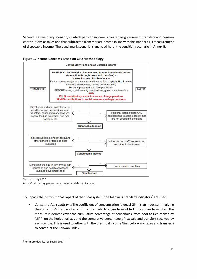
3 Methodology To analyze the distributional impact of the fiscal system in Croatia, we follow the CEQ methodology developed by Lustig (2017) and colleagues. It is based on income concepts that may or may not include specific fiscal interventions (Figure 1) to assess how the system and specific interventions affect poverty and inequality. We apply this approach to answer the following questions: How much does the fiscal system contribute to changing market income inequality? Does it help reduce poverty? Which taxes and transfers are progressive or pro-poor? What would be the distributional impact of specific fiscal interventions? In this analysis, the following income concepts apply:

Market income includes gross income, such as wages, salaries, income from capital assets (rent, interest, dividends), and private transfers before taxes and social contributions (remittances and other private transfers, such as alimony).

Market income plus pensions (MIPP) is the sum of market income and the subsidized portion of income from contributory pensions.

Disposable income is constructed by adding direct transfers to and subtracting direct taxes and social contributions from market income. Croatia’s direct taxes include the PIT, surtaxes, and taxes on vessels, road motor vehicles, and vacation homes.

Consumable income subtracts indirect taxes from disposable income. Croatia’s indirect taxes analyzed here are the VAT; excises on alcohol, tobacco, fuel, and automobiles; and other indirect taxes not classified as VAT or excises.

Final income adds to consumable income benefits in the form of social spending on health and education.

Because so much depends on the design and functions of the pension system in each country, there is no consensus in the literature on how to treat contributory pensions and related contributions. There are usually two scenarios. One is the benchmark scenario where old-age pension income is treated as deferred income and therefore added to market income, and pension contributions are treated as savings.

11

Second is a sensitivity scenario, in which pension income is treated as government transfers and pension contributions as taxes and thus subtracted from market income in line with the standard EU measurement of disposable income. The benchmark scenario is analyzed here, the sensitivity scenario in Annex B.

Figure 1. Income Concepts Based on CEQ Methodology

Source: Lustig 2017. Note: Contributory pensions are treated as deferred income.

To unpack the distributional impact of the fiscal system, the following standard indicators8 are used:

Concentration coefficient: The coefficient of concentration (a quasi-Gini) is an index summarizing the concentration curve of a tax or transfer, which ranges from –1 to 1. The curves from which the measure is derived cover the cumulative percentage of households, from poor to rich ranked by MIPP, on the horizontal axis and the cumulative percentage of tax paid and transfers received by each centile. This is used together with the pre-fiscal income Gini (before any taxes and transfers) to construct the Kakwani index.

8 For more details, see Lustig 2017.

12

Kakwani index: This is a useful measure of progressivity. The Kakwani index for taxes is defined as the difference between the concentration coefficient of the tax and the Gini for pre-fiscal income; for transfers, it is defined as the difference between the Gini for pre-fiscal income and the concentration coefficient of the transfer. A Kakwani index rating will be positive if a tax is globally progressive, negative if it is regressive. A rating for transfers is positive if a transfer is progressive in relative terms.9

Redistributive effect: This indicator captures the marginal contribution of the fiscal system to the Gini coefficient of inequality. The marginal contribution is understood as the difference between the Gini coefficient with and without the tax or transfer.10 If positive, it captures a redistributive effect, so the Gini declines.

Poverty reduction effect: This captures the marginal contribution of the fiscal system element(s) to poverty defined at a certain poverty line. Again, the marginal contribution is understood as the difference between the poverty rate with and without the tax or transfer. If positive, it captures a poverty reduction effect, so poverty declines.

Note that a progressive tax does not necessarily reduce inequality,11 which would be a positive redistribution effect, or poverty, a positive poverty reduction effect. And a tax can reduce inequality but at the same time increase poverty.12 For a complete picture, measures of progressivity must therefore be combined with marginal contributions to evaluate the effects of fiscal interventions on poverty and inequality.

4 Data and the Empirical Strategy for the Analysis 4.1 Household Survey Data

The analysis uses data from the Croatian HBS for 2017 and the SILC for 2019, which deals with household income in 2018. The HBS, conducted every three years, provides valuable information on the socio-economic situation of Croatian households, as well as collecting income and expenditure data. The 2017 HBS covered 1,377 households and is representative of the resident population outside hospitals, nursing homes, prisons, and other such institutions. Although the HBS reports household income and benefits, it is not as detailed as the SILC. For example, the 2017 HBS reports only total household income after taxes and cash transfers. The SILC 2019 disaggregates household income into wage income of employees, income of self-employed persons, property and capital income, and old-age pensions, and gives details of

9 A tax is globally progressive if the proportion paid in relation to pre-fiscal income increases as income rises. This happens when the concentration curve is completely below the pre-fiscal income Lorenz curve. A transfer is globally progressive in relative terms if the proportion received in relation to pre-fiscal income decreases as income rises. This happens when the concentration curve lies between the pre-fiscal income Lorenz curve and the 45-degree line. 10 Note that there is path dependence in estimating these marginal contributions, since the order in which each intervention is considered matters for the magnitude of the estimated marginal contribution. The estimation approach uses a Shapely decomposition to address this issue, which involves estimating marginal contributions in every possible path and then taking the average. 11 In the literature, this is known as the Lambert conundrum (Lambert 2001; Lustig 2017). Taxes, for instance, can be regressive according to the Kakwani index but when combined with transfers make the system more equalizing than without the regressive taxes. For a thorough discussion see Enami, Lustig, and Aranda 2017. 12 See Higgins and Lustig 2016.

13

social assistance benefits. Moreover, because the 7,880-household SILC sample is much larger it better captures variations in household types to interpret how fiscal interventions affect income distribution. As a result, this analysis is primarily based on the 2019 SILC and uses income as a basic measure for analysis.

We start with setting market income equal to gross income reported in the 2019 SILC. In our benchmark scenario, old-age pensions are treated as deferred income, and thus included in market income, now labelled MIPP. However, market income includes only non-pension contributions, not contributions for pension insurance.

From MIPP, we obtain disposable income by removing direct taxes and non-pension social insurance contributions and adding direct transfers, excluding old-age pensions. To construct consumable income, we deduct indirect taxes (VAT and excises) from disposable income. However, indirect taxes are based on consumption, data for which are available only in the 2017 HBS. We therefore simulate indirect taxes in the HBS and then apply survey-to-survey imputation to assign them to each SILC household (see Annex C for details). Finally, we add social spending on health and education to obtain final income.

The analysis is complemented by data from national and other public finance accounts from the Croatian Bureau of Statistics (CBS) and the MOF. This includes information on consolidated government budgets, local government budgets, and CBS annual reports on various sectors. Eurostat is the source for the input-output table for the Croatian economy and the figures on government spending by function.

To estimate the impacts of fiscal interventions on poverty, we use two poverty lines: the international line at $5.50 per person per day at the 2011 revised PPP, and the national at-risk-of-poverty (AROP) threshold, which is set at 60 percent of median equivalized household disposable income. For sensitivity analysis, we also use several other poverty lines and report their results in Annex D.

4.2 Fiscal Instruments

For revenues, the analysis covers PIT, social insurance contributions, and indirect taxes. Within indirect taxes, we include VAT and excises on tobacco products, alcohol, coffee and other nonalcoholic beverages, oil derivatives (petrol, diesel, etc.), and electricity. However, excises on imported motor vehicles and other taxes are excluded due to lack of data. Items analyzed here account for about 75 percent of total government revenue.

On spending, the analysis covers social protection programs like old-age pensions and child benefits plus spending on health and education. In 2018 these accounted for 48 percent of total spending. At least in the short term, other spending categories, such as national security and public order, are likely to be less relevant from a distributional impact perspective.

4.3 Empirical Strategies and Assumptions

As described in section 4.1, we use data from the 2017 HBS and the 2019 SILC data, which refers to household income in 2018. Since household data are often several years old, a nowcasting method can be used to extrapolate from data of the recent past, here 2018, to reflect the present situation. This method has been applied in the CEQs for such countries as Mexico, Argentina, and Armenia (Scott 2013, Rossignolo 2017, Younger and Khachatryan 2014), and in other microsimulation models, such as FiscalSim. A major caveat is that GDP growth is used to update the model, e.g., from 2018 to 2020, and assumes a

14

neutral distribution of growth. As constructed, it does not capture reforms introduced during the period that may not be reflected in GDP growth, such as parental benefits. Moreover, it does not account for differences in how reforms affect people across the income distribution.

Instead of using nowcasting, we base our model in 2018, which reflects the distributional impacts of the fiscal system in 2018. We then simulate the impacts of tax and social assistance reforms introduced between 2018 and 2021 on inequality and poverty.13 (See section 7.1 for details of the reforms.) The empirical strategy is discussed below, together with assumptions for matching household-level data with fiscal accounts and for overcoming problems arising from the microdata available.

Personal Income Taxes and Social Insurance Contributions

For PIT, we apply the statutory rates on gross income from employment, self-employment, pensions, and capital. One challenge we have is identifying in the 2019 SILC specific demographic groups that qualify for special PIT treatment. The first group is self-employed farmers who are exempted from the PIT. The SILC has no identifying information and there is no public data on the share of farmers eligible for exemption. We thus assume that each farmer has a 25 percent chance of paying the PIT. The second group is people who have income from contractual work, for whom the PIT rate is a flat 24 percent. Since there are no specific SILC data, we assume these people are self-employed and apply that rate.

Another challenge is the surtax from local governments (towns and municipalities), for which SILC data does not allow geographic identification. We therefore apply a rate of 9.42 percent, which is equivalent to the population-weighted average of all surtax rates. Finally, to determine the total personal PIT allowance—a tax deduction equal to a basic allowance for a taxpayer plus additional allowances for dependents—we assume that only one member per household claims the entire additional allowance for dependents in the household. This taxpayer is typically the one with the highest gross income.

For social security contributions, we apply 20 percent pension contributions for wage-earners. We also assume that social contributions paid by employers (general health, occupational health, and employment) fall fully on the employees. For the self-employed, the SIC base is the national average wage from January to August of the previous year plus a multiplier based on the type of self-employment (farmers, lawyers, craftsmen, etc.).14 However, the SILC data only distinguish two types of self-employment: farmers and nonfarmers. Since craftsmanship is the most common type of nonfarm self-employment in Croatia, we apply the multiplier for that to all nonfarm self-employed workers. For farmers, the contribution rates depend on whether they are exempt from the PIT. As discussed, we assume each farmer has a 25 percent probability of paying the PIT and estimate the SIC accordingly. We also calculate the general health contribution for pensioners, applying two different rates depending on their gross pension relative to the national average net wage from January to August of the previous year.

Pensions and Social Protection Spending

The analysis covers both the old-age contributory pensions and income from certain social protection programs. Old-age pension income is treated as deferred income and pension contributions as savings. Thus, pension income is part of the MIPP, but not pension contributions. However, the results for the

13 The simulation is based on 2018 prices. 14 For nonfarmers, the multiplier is either 1.1 (for professionals such as lawyers, tax advisors, architects, etc.) or 0.65 (for craftsmen and professionals like journalists, physiotherapists, etc.).

15

sensitivity scenario, in which pension income is considered government transfers and pension contributions are treated as taxes are presented in Annex B. We treat survivor-related benefits like old-age pensions instead of a separate transfer, assuming that most survivors inherit the old-age pension of a deceased family member.

Social protection programs that are government cash transfers covered in the analysis are unemployment, maternity leave, and parental leave benefits; maternity and parental allowances; grants for each newborn child; the child benefit; the guaranteed minimum benefit; compensation for electricity cost; education-related and housing-related benefits; sickness benefit; and disability pension and benefits. For each program, we apply eligibility criteria to simulate the benefits received rather than using the amount reported in the SILC data. There are two reasons for this approach: (1) The amount received is severely under-reported in the SILC. Aggregated for the whole country, the amounts reported cannot be matched with the administrative data. (2) Using the amount reported does not allow us to simulate the distributional impacts of social spending reforms without changing the parameters of interest. (Annex A provides details.) However, the SILC does not provide enough information to impute the amount received from education-related, housing-related, sickness benefits, and disability pensions and benefit. Thus, for these four programs, we must use the amounts reported in the SILC.

Indirect Taxes

The indirect taxes analyzed here are the VAT and excises. Because the necessary data are not available, sales and other taxes and excises on cars, other motor vehicles, vessels, and airplanes, and luxury products are excluded. The VAT paid by government is also excluded, not only because the data are not available but also because it has limited relevance to household income. Since the SILC data do not contain household consumption expenditures, which are the basis for estimating indirect taxes, the VAT and excises are first simulated, using expenditure information in the HBS data, then imputed into the SILC using a survey-to-survey imputation method (see Annex C for more information).

For both the VAT and excises, the exercise captures the direct effects—the amounts paid directly by households when purchasing locally manufactured and specific imported goods subject to these taxes—plus the indirect effects that taxes on petrol, diesel fuels, and electricity may have on product prices. The indirect effects are estimated using an input-output matrix for the Croatian economy to map household consumption from the HBS to the input-output production sectors. The analysis does not consider the possibility of evasion of either the VAT or excises.

Social Spending on Health and Education

On education, the SILC provides information on the number of children in each household attending school and at which level of education (pre-primary and primary; secondary and post-secondary non-tertiary; and tertiary). Thus, for each student, we estimate the amount of education benefits equivalent to government spending per student by level. We obtain the number of students in 2018 from the CBS and obtain from the Eurostat (2021) Classification of the Functions of Government (COFOG) government spending (administrative costs, recurring expenditures, and investment) by level of education.

For health, we obtain government spending by type of services, using the COFOG classification to disaggregate spending by medical products, appliances, and equipment; outpatient services; hospital services; and public health and other services. Unfortunately, SILC data does not allow us to identify

16

individuals who may be using each type. We therefore assume that each Croatian receives health benefits equivalent to average government spending per capita.

The analysis does not capture differences in the quality of the services provided. Nor does it reflect variation in the value of these services across the income distribution.

4.4 Macro Validation

We assess the performance of the model and its assumptions by comparing the aggregate amount of each tax and transfer captured in the analysis with the same category from the official statistics (see Annex E for details). It is critical to evaluate whether the relative magnitude of the fiscal instruments represented by the SILC and the HBS is comparable to that in the economy. This exercise shows that the model performs relatively well. For all fiscal instruments together, the average ratio of the simulated to the actual amount is 0.84; in other words, the model captures on average 84 percent of the value of taxes and social transfers in the official statistics. The model performs particularly well for such important interventions as the PIT and VAT, but less so, mostly due to incomplete data, on excises and SIC on income from self-employment.

4.5 Caveats

There are a couple of caveats. First, the analysis focuses on short-term impacts of fiscal and social policies but not on their potential long-term effects on productivity, employment, and income. For example, excise taxes could be regressive and poverty increasing in the immediate term but some excise taxes, in particular taxes on tobacco products and sugar-sweetened beverages, may have positive indirect benefits for the poor in the long run by improving health outcomes and labor productivity (Fuchs and Icaza 2021, World Bank 2020). Second, as in any survey-based analysis, our model relies on the quality and comprehensiveness of the SILC and the HBS. In some cases, the survey data do not provide sufficient information to accurately apply the specificities of the fiscal instruments such as identification of self-employed farmers exempted from the PIT and eligibility criteria for disability benefits. Annex A details these issues under “modeling notes”. Third, informality and evasion of taxes and social insurance contributions are not taken into account due to lack of data. While the recent amount of evasion is not available, previous estimates suggest that it could be equivalent to 5.9 percent of GDP (Madžarević-Šujster 2002). Finally, the analysis does not capture the consequences of the economic crisis brought about by the COVID-19 pandemic since 2020. The distributive impacts of the crisis on public finances, on both the revenue and expenditure sides, and on household welfare remain to be examined when survey data become available.

5 Results: Distributional Impact of the Fiscal System in Croatia 5.1 Impacts on Inequality

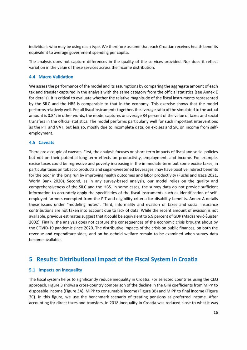
The fiscal system helps to significantly reduce inequality in Croatia. For selected countries using the CEQ approach, Figure 3 shows a cross-country comparison of the decline in the Gini coefficients from MIPP to disposable income (Figure 3A), MIPP to consumable income (Figure 3B) and MIPP to final income (Figure 3C). In this figure, we use the benchmark scenario of treating pensions as preferred income. After accounting for direct taxes and transfers, in 2018 inequality in Croatia was reduced close to what it was

17

in 2014 and comparable to the level in Poland. In Croatia the redistributive effect through direct taxes and transfers was much higher than in Belarus, Montenegro, Romania, and Russia, with most of the reduction in inequality driven by pensions (Figure 3A). However, once indirect taxes are taken into account, the equalizing effects in Croatia are only the second lowest after Montenegro (Figure 3B). Nevertheless, social spending on health and education in Croatia significantly reduces inequality, making it the best performer among peers (Figure 3C).

Figure 2 shows changes in Gini coefficients from household MIPP, which treats pensions as deferred income, to disposable income (subtracting direct taxes and contributions and adding direct transfers), to consumable income (removing indirect taxes), and to final income (adding in-kind transfers).

Before any fiscal interventions, the Gini coefficient holds at 0.474 if old-age contributor pensions are treated as government transfers, and 0.360 if pensions are considered deferred income; that suggests that pensions have substantial equalizing effects. Once direct taxes, social security contributions, and direct transfers are taken into account, inequality goes down to 0.297. However, the non-equalizing effects of indirect taxes (VAT and excises) drive the Gini index up to 0.326. The largest decline in inequality comes from social spending on health and education, which pushes the Gini coefficient down to 0.238 for household final income. The total reduction in inequality from household MIPP to final income was as low as 0.122 Gini points when old-age contributory pensions are treated as deferred income and as high as 0.236 when pensions are treated as government transfers.

For selected countries using the CEQ approach, Figure 3 shows a cross-country comparison of the decline in the Gini coefficients from MIPP to disposable income (Figure 3A), MIPP to consumable income (Figure 3B) and MIPP to final income (Figure 3C). In this figure, we use the benchmark scenario of treating pensions as preferred income. After accounting for direct taxes and transfers, in 2018 inequality in Croatia was reduced close to what it was in 2014 and comparable to the level in Poland. In Croatia the redistributive effect through direct taxes and transfers was much higher than in Belarus, Montenegro, Romania, and Russia, with most of the reduction in inequality driven by pensions (Figure 3A). However, once indirect taxes are taken into account, the equalizing effects in Croatia are only the second lowest after Montenegro (Figure 3B). Nevertheless, social spending on health and education in Croatia significantly reduces inequality, making it the best performer among peers (Figure 3C).

Figure 2. Inequality from Market to Final Income (Gini Coefficient)

Source: Authors’ estimates.

0.360

0.2970.326

0.238

0.474

0.2970.326

0.238

Pre-fiscal income Disposable income Consumable income Final income

Pensions as deferred income Pensions as government transfer

18

Figure 3. Cross-country Comparison: Change in Inequality, Measured by Gini Coefficients

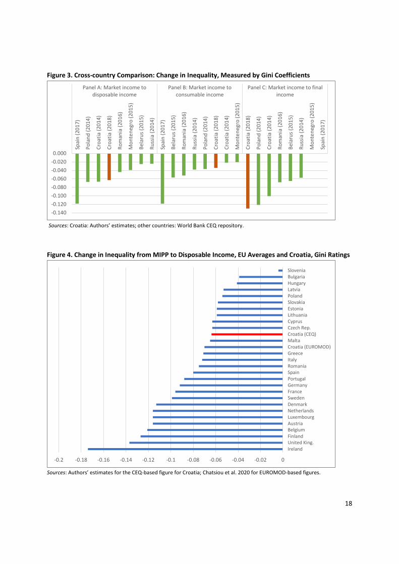
Sources: Croatia: Authors’ estimates; other countries: World Bank CEQ repository. Figure 4. Change in Inequality from MIPP to Disposable Income, EU Averages and Croatia, Gini Ratings

Sources: Authors’ estimates for the CEQ-based figure for Croatia; Chatsiou et al. 2020 for EUROMOD-based figures.

-0.140-0.120-0.100-0.080-0.060-0.040-0.0200.000

Spai

n (2

017)

Pola

nd (2

014)

Croa

tia (2

014)

Croa

tia (2

018)

Rom

ania

(201

6)

Mon

tene

gro

(201

5)

Bela

rus (

2015

)

Russ

ia (2

014)

Spai

n (2

017)

Bela

rus (

2015

)

Rom

ania

(201

6)

Russ

ia (2

014)

Pola

nd (2

014)

Croa

tia (2

018)

Croa

tia (2

014)

Mon

tene

gro

(201

5)

Croa

tia (2

018)

Pola

nd (2

014)

Croa

tia (2

014)

Rom

ania

(201

6)

Bela

rus (

2015

)

Russ

ia (2

014)

Mon

tene

gro

(201

5)

Spai

n (2

017)

Panel A: Market income todisposable income

Panel B: Market income toconsumable income

Panel C: Market income to finalincome

-0.2 -0.18 -0.16 -0.14 -0.12 -0.1 -0.08 -0.06 -0.04 -0.02 0

IrelandUnited King.FinlandBelgiumAustriaLuxembourgNetherlandsDenmarkSwedenFranceGermanyPortugalSpainRomaniaItalyGreeceCroatia (EUROMOD)MaltaCroatia (CEQ)Czech Rep.CyprusLithuaniaEstoniaSlovakiaPolandLatviaHungaryBulgariaSlovenia

19

5.2 Impacts on Poverty

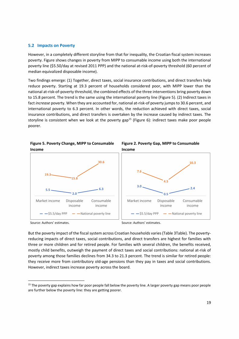
However, in a completely different storyline from that for inequality, the Croatian fiscal system increases poverty. Figure shows changes in poverty from MIPP to consumable income using both the international poverty line ($5.50/day at revised 2011 PPP) and the national at-risk-of-poverty threshold (60 percent of median equivalized disposable income).

Two findings emerge: (1) Together, direct taxes, social insurance contributions, and direct transfers help reduce poverty. Starting at 19.3 percent of households considered poor, with MIPP lower than the national at-risk-of-poverty threshold, the combined effects of the three interventions bring poverty down to 15.8 percent. The trend is the same using the international poverty line (Figure 5). (2) Indirect taxes in fact increase poverty. When they are accounted for, national at-risk-of poverty jumps to 30.6 percent, and international poverty to 6.3 percent. In other words, the reduction achieved with direct taxes, social insurance contributions, and direct transfers is overtaken by the increase caused by indirect taxes. The storyline is consistent when we look at the poverty gap15 (Figure 6): indirect taxes make poor people poorer.

Figure 5. Poverty Change, MIPP to Consumable Income

Figure 2. Poverty Gap, MIPP to Consumable Income



But the poverty impact of the fiscal system across Croatian households varies (Table 3Table). The poverty-reducing impacts of direct taxes, social contributions, and direct transfers are highest for families with three or more children and for retired people. For families with several children, the benefits received, mostly child benefits, outweigh the payment of direct taxes and social contributions: national at-risk of poverty among those families declines from 34.3 to 21.3 percent. The trend is similar for retired people: they receive more from contributory old-age pensions than they pay in taxes and social contributions. However, indirect taxes increase poverty across the board.

15 The poverty gap explains how far poor people fall below the poverty line. A larger poverty gap means poor people are further below the poverty line: they are getting poorer.

5.52.0

6.3

19.315.8

30.6

Market income Disposableincome

Consumableincome

$5.5/day PPP National poverty line

3.0

0.5

2.4

7.6

4.5

10.3

Market income Disposableincome

Consumableincome

$5.5/day PPP National poverty line

20

Table 3. Poverty Trajectory from MIPP to Consumable Income, by Household Type

Household Type

Market Income

plus Pension

Disposable Income

Consumable Income

Market Income

plus pension

Disposable Income

Consumable Income

National at risk of poverty threshold International poverty line No children 11.3 12.7 24.4 5.7 3.3 7.0 1 or 2 children 12.3 12.5 26.2 2.8 1.7 6.1 3 or more children 34.3 21.3 40.6 21.1 6.7 15.4 Single retiree 42.7 40.2 64.3 4.0 0.2 4.0 Retired couple 14.4 8.3 29.4 1.6 0.1 0.4 Urban 15.0 12.5 26.4 4.0 1.5 4.4 Rural 26.3 21.3 37.5 7.9 2.9 9.4


6 Incidence, Progressivity, and Marginal Contributions of Taxes and Social Spending After the Section 5 assessment of how the fiscal system as a whole impacts inequality and poverty, this section examines the distributional impact—the extent to which the fiscal system affects household income across the welfare distribution. Moreover, for each instrument of the fiscal system, the analysis looks at its contributions to changes in poverty, the poverty reduction effect, and inequality, the redistributive effect. To do so, we study the marginal effect16 of each fiscal instrument on the Gini coefficient and on poverty. In general, an instrument would have a significant distributional impact if it is targeted to people at the bottom of the income distribution (as captured by the concentration coefficients) and its generosity is relatively large compared to recipient incomes.

6.1 Distributional Profile of the Fiscal System

Before taking a closer look at each instrument, we assess the distributional impacts of the fiscal system as a whole. We first divide MIPP into deciles, with households in the first decile being the poorest and those in the tenth the richest.

Figure 7 shows the share of MIPP of different components of the tax and benefit system by decile. Most components of the fiscal system are progressive, with the poorest being net receivers of social benefits, as shown by their positive net cash position.17 The share of each component is large for households in the bottom decile because the MIPP of the poorest is very low, so payments of taxes or the amount of benefits are relatively substantial. However, starting at the second decile, Croatian households are net payers to the Treasury—direct and indirect taxes paid exceed cash benefits received. The net cash position is negative for all but the poorest 10 percent of the population. But when health and education are taken

16 The marginal effect is the change in market income by adding or subtracting only the given element. 17 The net cash position captures the difference between market income and consumable income (equivalent to net payment of direct and indirect taxes, and cash benefits) as a share of market income.

21

into account, households in the bottom 40 percent of the income distribution are net receivers because the share of cash and in-kind benefits together outweighs the tax payments (net total position18 is positive for the bottom four deciles). The curve of the net total position (the black line in Figure 7) depicts a decreasing trend, from the poorest receiving net benefits equivalent to 212 percent of their income to the richest paying about 27 percent of their income into the fiscal system.

Figure 7. Taxes and Benefits by Decile, MIPP

Source: Authors’ estimates. Notes: SIC: Social Insurance Contributions. The net total position is the difference between final income and MIPP. The net cash position is the difference between consumable income and MIPP.

A fundamental question for policy makers is whether a specific fiscal instrument or combination of them, is equalizing, since the impact of an instrument may be different from that of the whole system. To answer this question, the analysis relies on the concepts defined in Section 3: progressivity (Kakwani index); marginal contributions to inequality (redistributive effect); and poverty (poverty-reducing effect). If there was a single fiscal instrument, using indicators like the Kakwani index would be sufficient to determine its progressivity or regressivity. However, in reality, there are often multiple fiscal instruments, so the one-to-one relationship between the progressivity of an intervention and its effect on inequality no longer holds as each instrument interacts with all the others. In this case, we can use marginal contributions to inequality to examine the marginal effect of a particular fiscal instrument on inequality.

Table 4 shows both the Kakwani progressivity index for each tax and transfer and its marginal contribution to reducing inequality and poverty19 in the benchmark scenario, where old-age contributory pensions are

18 The net total position captures the difference between income and final income (equivalent to net payment of direct and indirect taxes, cash and in-kind benefits) as a share of market income. A household is a net receiver of the fiscal system when its net total position is positive and a net payer when its net position is negative. 19 Poverty measures are defined as a share of population living below $5.50 a day at the revised 2011 PPP.

-150

-100

-50

0

50

100

150

200

250

300

350

1 2 3 4 5 6 7 8 9 10

% o

f MIP

P

MIPP-based decile

Education

Health

Indirect taxes

Non-pension SIC

Direct transfers

Direct taxes

Net total position

Net cash position

22

treated as deferred income. (See Annex B for results of the sensitivity scenario.) The following sections discuss the results of each instrument. The effect also depends on the magnitude of each instrument (Table 4, column 1) with respect to a household’s MIPP.

Table 4. Progressivity and Marginal Contributions of Fiscal Instruments

Percent of

MIPP*

Concentration Coefficient (with Respect to MIPP)

Kakwani index

Marginal Contributions

Redistributive Effect

Poverty Reduction

Effect (1) (2) (3) (4) (5) Disposable Income Direct taxes –6.94 0.6843 0.3240 0.0259 0.0000 Personal income tax and surtax –6.82 0.6887 0.3284 0.0258 0.0000 Property taxes –0.12 0.4378 0.0774 0.0002 0.0000 Non-pension social insurance contributions –10.92 0.3579 –0.0025 0.0025 –0.7700 Direct transfers 6.20 –0.4730 0.8333 0.0409 4.7081 Unemployment benefit 0.33 –0.3105 0.6708 0.0019 0.1986 Maternity leave benefit 0.30 –0.0486 0.4089 0.0009 0.0000 Parental leave benefit 0.30 –0.2272 0.5876 0.0016 0.0000 Maternity and parental allowance 0.29 –0.5697 0.9300 0.0027 0.1886 Grant for newborn child 0.04 –0.1801 0.5404 0.0002 0.0000 Child benefit 0.77 –0.7270 1.0873 0.0090 0.9991 Guaranteed minimum benefit 0.25 –0.9504 1.3107 0.0034 0.7163 Compensation for electricity cost 0.05 –0.9179 1.2783 0.0006 0.1155 Education-related benefits 0.18 –0.0163 0.3766 0.0006 0.0607 Sickness benefit 0.26 –0.1457 0.5061 0.0010 0.0901 Disability pension & benefits 3.39 –0.4875 0.8478 0.0166 1.7081 Housing-related benefits 0.05 –0.8317 1.1920 0.0006 0.0981 Consumable Income Indirect taxes –17.83 0.1670 -0.1933 -0.0301 -4.2853 Value added tax –14.97 0.1661 -0.1942 -0.0260 -4.0256 Excises –2.86 0.1718 -0.1885 -0.0062 -1.1411 Final Income In-kind benefits 24.89 -0.0454 0.4057 0.0885 Health 13.42 0.0000 0.3603 0.0389 Products, appliances, and equipment 3.17 0.0000 0.3603 0.0082 Outpatient services 2.19 0.0000 0.3603 0.0056 Hospital services 6.74 0.0000 0.3603 0.0181 Public health and other 1.32 0.0000 0.3603 0.0033 Education 11.47 –0.0985 0.4588 0.0363 Pre-primary and primary 6.81 –0.1636 0.5240 0.0272 Secondary and post-secondary non-tertiary 2.04 -0.1860 0.5463 0.0082 Tertiary 2.61 0.1400 0.2203 0.0014

Source: Authors’ estimates. Notes: MIPP: Market income plus pensions. As is customary, the poverty reduction effects of in-kind benefits are not considered. 6.2 Direct Taxes, Indirect Taxes, and Social Insurance Contributions

Direct taxes are progressive, have equalizing effects, but have no impact on poverty. The Kakwani coefficients are positive, indicating progressivity, and highest for the PIT at 0.328 (Table 4, column 2, and Figure 9). The PIT is also very concentrated, with richer people paying a larger share of the total collected:

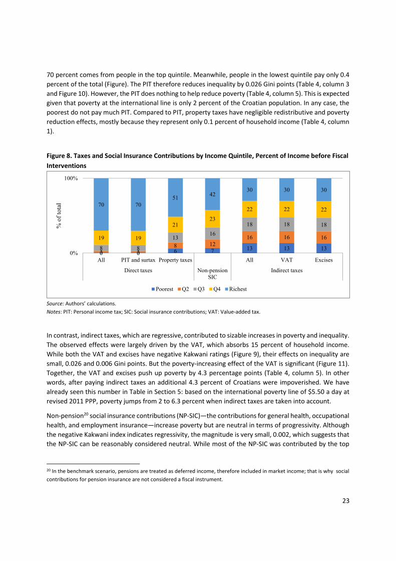
23

70 percent comes from people in the top quintile. Meanwhile, people in the lowest quintile pay only 0.4 percent of the total (Figure). The PIT therefore reduces inequality by 0.026 Gini points (Table 4, column 3 and Figure 10). However, the PIT does nothing to help reduce poverty (Table 4, column 5). This is expected given that poverty at the international line is only 2 percent of the Croatian population. In any case, the poorest do not pay much PIT. Compared to PIT, property taxes have negligible redistributive and poverty reduction effects, mostly because they represent only 0.1 percent of household income (Table 4, column 1).

Figure 8. Taxes and Social Insurance Contributions by Income Quintile, Percent of Income before Fiscal Interventions

Source: Authors’ calculations. Notes: PIT: Personal income tax; SIC: Social insurance contributions; VAT: Value-added tax.

In contrast, indirect taxes, which are regressive, contributed to sizable increases in poverty and inequality. The observed effects were largely driven by the VAT, which absorbs 15 percent of household income. While both the VAT and excises have negative Kakwani ratings (Figure 9), their effects on inequality are small, 0.026 and 0.006 Gini points. But the poverty-increasing effect of the VAT is significant (Figure 11). Together, the VAT and excises push up poverty by 4.3 percentage points (Table 4, column 5). In other words, after paying indirect taxes an additional 4.3 percent of Croatians were impoverished. We have already seen this number in Table in Section 5: based on the international poverty line of $5.50 a day at revised 2011 PPP, poverty jumps from 2 to 6.3 percent when indirect taxes are taken into account.

Non-pension20 social insurance contributions (NP-SIC)—the contributions for general health, occupational health, and employment insurance—increase poverty but are neutral in terms of progressivity. Although the negative Kakwani index indicates regressivity, the magnitude is very small, 0.002, which suggests that the NP-SIC can be reasonably considered neutral. While most of the NP-SIC was contributed by the top

20 In the benchmark scenario, pensions are treated as deferred income, therefore included in market income; that is why social contributions for pension insurance are not considered a fiscal instrument.

0 0 6 7 13 13 133 38 12

16 16 16

8 8

1316

18 18 18

19 19

2123

22 22 2270 70

51 4230 30 30

0%

100%

All PIT and surtax Property taxes All VAT Excises

Direct taxes Non-pensionSIC

Indirect taxes

% o

f tot

al

Poorest Q2 Q3 Q4 Richest

24

income quintiles, 7 percent of the total still comes from the pockets of the poor (Figure 8). The NP-SIC indeed increases poverty by 0.77 pp (Figure 11).

Figure 9. Progressivity of Taxes and Contributions (Kakwani Index)

Source: Authors’ estimates. Figure 10. Redistributive Effects

Source: Authors’ estimates. Figure 11. Poverty Reduction Effects, Percentage Points


0.328

0.077

-0.002

-0.194 -0.189-0.300-0.200-0.1000.0000.1000.2000.3000.400

PIT Property taxes VAT Excises

Direct taxes Non-pensioncontributions

Indirect taxes

Kakw

ani i

ndex

0.026

0.000 0.003

-0.026

-0.006

-0.030-0.020-0.0100.0000.0100.0200.030

PIT Property taxes Value added tax Excises


Indirect taxes

Chan

ge in

GIn

i

0.000 0.000

-0.770

-4.026

-1.141

-5.000-4.000-3.000-2.000-1.0000.0001.000

PIT Property taxes Value added tax Excises


Indirect taxes

Chan

ge in

pov

erty

(% p

oint

)

25

6.3 Direct and In-kind Transfers

All direct transfers are progressive, and to different extents have positive effects on redistributive and poverty-reducing efforts. Disability pensions and benefits and child benefits are the largest as shares of household income (Table 4, Column 1). Other individual programs each contribute less than 0.5 percent of household income. The positive Kakwani index shows progressivity for all direct transfers. As a group, direct transfers are pro-poor, with households in the bottom quintile receiving 54 percent and those in the top quintile just 5 percent. But the concentration varies by program (Figure 12). As would be expected, low-income support, such as the guaranteed minimum benefit or the compensation for electricity costs, target almost exclusively households in the bottom income quintile. Maternity and parental leave benefits and education-related benefits are less concentrated because they are not designed to be pro-poor. Despite this variation, the concentration coefficients are all negative (Table 4, Column 2). indicating that there is no benefit the rich receive more than the poor. All direct transfers together help reduce inequality by 0.04 Gini points (Figure 14) and poverty by 4.7 pp (Figure 15). It is important to note that the poverty-reducing effect of direct transfers exceeds the poverty-increasing effect of direct taxes and social contributions. As a result, poverty declines from 5.5 to 3.0 percent when moving from MIPP to disposable income (Figure 5Figure).

Among direct transfers, the most equalizing and poverty-reducing programs are disability pensions and related benefits, child benefits, and guaranteed minimum benefits (Figures 14 and 15). Even though they are not poverty-targeted directly, because disability pensions constitute 3.4 percent of household income and child benefits 0.8 percent, they have larger poverty impact, the pensions-related benefits help to reduce poverty by 1.7 pp and the child benefits do so by 1 pp (Figure 15). The main poverty-alleviation program, the guaranteed minimum benefit, has less impact on poverty and inequality because at only 0.25 percent of household income it is relatively small. Its distributive effect comes mainly from its progressivity (the highest Kakwani index)— it is well targeted to the poorest.

Figure 12. Direct Cash Transfers by Income Quintile, Percent of MIPP

Source: Authors’ estimates. Note: MIPP: Market income plus pensions.

1855

3440

879799

97

7530

6820

1853

54

0% 100%

Education-related benefitsDisability pensions and benefits

Sickness benefitUnemployment benefit

Housing-related benefitsCompensation for electricity costs

Guaranteed minimum benefitAll low income support benefits

Child benefitGrant for newborn children

Maternity and parental allowanceParental leave benefit

Maternity leave benefitAll family- and child- related benefits

All direct transfers

% of total


26

Figure 13. Progressivity of Direct Transfers (Kakwani Index)

Source: Authors’ estimates. Figure 14. Redistributive Effect of Direct Transfers


0.0 0.2 0.4 0.6 0.8 1.0 1.2 1.4

All direct transfers Unemployment benefit Maternity leave benefit

Parental leave benefit Maternity and parental allowance

Grant for newborn child Child benefit

Guaranteed minimum benefit Compensation for electricity cost

Education-related benefits Sickness benefit

Disability pension & benefits Housing-related benefits

Kakwani index

0.00 0.01 0.01 0.02 0.02 0.03 0.03 0.04 0.04 0.05

Direct transfers Unemployment benefit Maternity leave benefit






Change in Gini

27

Figure 15. Poverty Reduction Effects of Direct Transfers


In-kind benefits—public spending on health and education—are progressive and equalizing (this analysis does not assess quality or efficiency). Benefits from public health and education amount to 24.9 percent of household income, the largest contribution the analysis found. The positive Kakwani rating indicates progressivity. In-kind benefits also help reduce inequality by 0.4 Gini points. However, because disposable income, used for poverty estimates, does not include in-kind benefits, their poverty-reducing effect is not evaluated.

Spending on public health is progressive and equalizing. However, it is important to take this conclusion with caution as we assume that each Croatian receives the same amount of government per capita spending due to data unavailability in the SILC (see section 4.3). Thus, by construction, the Kakwani index is equal to the Gini coefficient for MIPP, indicating progressivity. Spending on health, which constitutes 13.4 percent of household income, contributes to a reduction of 0.04 Gini point.

Similarly, spending on education is progressive and equalizing. Figure 3 shows that education spending is distributed relatively equally across quintiles, which implies widespread use of public education services in Croatia. Although the Kikwani index is positive across the board, spending on pre-primary, primary, secondary, and post-secondary education is more progressive than spending on tertiary (Figure 17).

Consistent with findings in other countries, the concentration coefficients of spending on lower levels of education are negative, suggesting that a larger share goes to students at the bottom of the income distribution. Since spending on pre-primary and primary education is relatively larger at 6.8 percent of household income, that has the largest redistributive role, reducing the Gini coefficient by 0.03 point (Figure 18).

0.0 0.5 1.0 1.5 2.0 2.5 3.0 3.5 4.0 4.5 5.0

Direct transfers Unemployment benefit Maternity leave benefit






Change in poverty (% point)

28

Figure 16. In-kind Transfers by Quintile, Percent of MIPP

Source: Authors’ estimates. Note: MIPP – Market income plus pensions

Figure 17. Progressivity of In-kind Transfers, Measured by the Kakwani Index

Figure 18. Redistributive Effect of In-kind Transfers



20 25 29 2911

2022 23 23

19

2020 20 21

20

2018 17 17

22

20 15 12 1027

0%

100%

Health spending Educationspending: all levels

Pre-primary andprimary education

Secondary andpost-secondary

non-tertiaryeducation

Tertiary education

% o

f tot

al


0.0 0.2 0.4 0.6

All in-kind benefits

Health spending

Education spending (all)

Education (pre-primaryand primary)

Education (secondary andpost-secondary)

Education (tertiary)

Kakwani index0.00 0.02 0.04 0.06 0.08 0.10

All in-kind benefits

Health spending

Education spending (all)

Education (pre-primaryand primary)

Education (secondaryand post-secondary)

Education (tertiary)

Change in Gini

29

7 Distributional Impacts of Tax and Social Spending Reforms, 2018 to 2021 In the previous two sections, where HBS and SILC data were available we analyzed the distributional impact of taxes and social spending in 2018. Between 2018 and 2021, the Government of Croatia introduced reforms of direct and indirect taxes, social insurance contributions, and direct cash transfers. Here, we simulate the distributional impact of these reforms, first describing the reforms analyzed and our simulation approach; and then analyzing how the reforms affected poverty and inequality.

7.1 Simulation Approach and Recent Reforms

Between 2018 and 2021, the government introduced reforms as series over time.21 We group them by type of instrument:

1. PIT-related reforms: With the goal of reducing the tax burden on workers, the government introduced a series of PIT reforms over the year. In January 2018, the lower limit of the top PIT bracket was increased from HRK 17,500 to HRK 30,000 per month, a relief of 71 percent. In January 2020, the basic personal allowance, a PIT deduction, was raised from HRK 3,800 to HRK 4,000 per month and tax relief for young people was introduced: workers younger than 25 were exempted from paying the PIT, and those aged 25–30 pay only 50 percent of the PIT obligation. These provisions applied only to the annual PIT base, below the lower limit of the top PIT bracket (HRK 30,000 per month). Most recently, in January 2021 all PIT rates were reduced, on the general schedule from 24 to 20 percent for the first bracket and from 36 to 30 percent for the top bracket. The rates for rental, interest, and capital income were also reduced, from 12 to 10 percent.

2. SIC reform: In January 2019, the occupational health SIC, formerly 0.5 percent, and the employment SIC, 1.7 percent, were abolished, and the general health was raised from 15 to 16.5 percent.

3. VAT reform: In January 2019, the standard VAT rate for fresh meat, fresh fish and seafood, fresh vegetables, fresh and dried fruits, and eggs was reduced from 25 to 13 percent.

4. Parental leave and child benefits reforms: In July 2018, the means test used to define whether households were eligible for the child benefit became more generous. The mount of household net income per capita, which determines whether a child receives the benefit, was raised by 40 percent, from HRK 1,663 to HRK 2,328.20. In principle, this allowed more households to meet the means test. As of April 2020, the maximum amount of the parental leave benefit was raised 42 percent, from HRK 3,991.20 to HRK 5,654.20.

5. National allowance for the elderly: In January 2021, the government introduced a new cash transfer, the national allowance for the elderly. Those eligible must meet the following criteria: they must be older than 65, retired, and a resident of Croatia for at least 20 years; they must not be receiving any pension or the guaranteed minimum benefit; and the net income per member of their household must not exceed HRK 800 a month. The monthly benefit is HRK 800, an amount to be adjusted for inflation over time.

21 For example, in 2018, the Government announced reforms to gradually lower the PIT burden over several years.

30

6. All reforms aggregated: A combination of reforms from group 1 to 5. It is important to consider the interactions among these groups, especially between the PIT/SIC reforms and the others. Because the PIT and SIC reforms could change household disposable income, they may affect household eligibility for some social transfer programs, such as child benefits and the new national allowance for the elderly. A change in disposable income may also affect the VAT paid by households through the consumption channel. For such reasons, the compound impact of all reforms on the budget, inequality, and poverty is not the sum of the impacts from individual reforms.

Table 5 presents the budgetary impact of these reforms. From the revenue side, reforms on PIT, SIC, and VAT will reduce the budget by 3.24, 0.33 and 1.11 billion HRK, respectively. From the fiscal spending side, reforms of parental leave and child benefits, and national allowance for the elderly would reduce the budget by another 0.67 billion HRK. The cumulative impact of these reforms taken together would cost about 5.3 billion HRK, or 1.4 percent of GDP.

Table 5. Simulated Budgetary Impact of Reforms Reform HRK billion % of GDP 1. PIT reforms -3.24 -0.85 2. SIC reform -0.33 -0.09 3. VAT reform -1.11 -0.29 4. Parental leave and child benefits reforms -0.60 -0.16 5. National allowance for the elderly -0.07 -0.02 6. All reforms aggregated -5.31 -1.39


7.2 Distributive Impact of Reforms

We first examine how the reforms change the net cash position—net payment of direct and indirect taxes and cash benefits as a share of MIPP—for households across the income distribution. In other words, we assess whether households receive more or less cash after each reform. Table 6, column 1 presents the pre-reform net cash position for households in each income decile. As discussed in section 6.1, only the poorest households in the bottom decile receive net cash (i.e., more in benefits than they pay in taxes); the rest are net payers to the Treasury. See Table 6, columns 2–7 for impacts of the reforms on household net cash positions . A positive number means the reform brings more cash to the household.

A reduction in PIT rates, an increase in the lower limit of the second PIT bracket, and tax relief for young workers would produce a net gain in cash for most households except those in the first decile (Table 6, column 2). However, for some of the poorest households, an increase in disposable income would disqualify them from some social assistance benefits, causing them a net loss of 0.15 percent of household income. Meanwhile, the richer the household, the more it benefits from the PIT-related reforms due to a larger cut in PIT rates for the top brackets and a reduction of the tax on rental and capital income.

Meanwhile, every household receives more cash from the SIC reforms (Table 6, column 3). On average, Croatians would receive cash equivalent to about 0.25 percent of their household income. The distribution is quite even across all households for two reasons: (1) The SIC reforms introduce the same change in

31

contribution rates for all workers. (2) The reforms do not affect the contribution base, household gross income.

The reduction in VAT rate for certain categories of food products also improves the net cash position of every household (Table 6, column 4), but especially poorer households, for which food takes up a larger budget share than for richer households. For example, households in the lowest decile would gain cash equivalent to 2.6 percent of their income, compared to 0.34 percent for those in the top quintile.

More generous programs on parental leave and child benefits also result in net gains for households in the lower part of the income distribution (Table 6, column 5). The higher income threshold for child benefits makes more people in the lower deciles eligible. A larger parental leave benefit for working parents results in more cash gains for those in the middle of the income distribution due to their employment status. While people in the top income deciles also enjoy parental leave benefits, the amount (raised from HRK 3,991.2 to HRK 5,654.20) is small relative to their income.

Finally, given the eligibility criteria, the national allowance for the elderly, can be expected to improve the net cash position for households in the poorest decile (Table 6, column 6). The cumulative impact of all reforms is to provide the most cash gains for the poorest and the richest (Table 6, column 7), with the poorest benefiting more from the VAT reforms and the richest from the PIT reforms.

The next question to be answered is: How have these reforms affected inequality in Croatia? Table 7 presents their impacts on the Gini coefficients for disposable income and consumable income. As explained in section 3, disposable income accounts for direct tax (PIT), SIC, and social cash transfers; consumption income takes into account all disposable income plus indirect taxes (VAT). Given the reforms analyzed we examines changes in the Gini coefficients for both income concepts. Table column 1 shows pre-reform Gini coefficients of 0.297 for disposable income and 0.326 for consumable income, as seen in section 5.1.

The PIT reforms increase inequality for both disposable and consumable income (Table 7, column 2) for two reasons: (1) The rich gain more from a deeper cut in PIT rates and the lower tax on rental and capital income. (2) The poor are worse off because they lose more from becoming ineligible for some social programs they gain from the PIT reduction.

The SIC reforms have no impact on inequality because the change in SIC rates applies uniformly to all workers (Table 7, column 3). The VAT reforms do slightly reduce, by 0.002 point, the Gini coefficient for consumable income22 (Table 7, column 4) because poor people, with food a relatively larger budget share, benefit more from a lower VAT on food items. The reforms of parental leave and child benefits lead to a small decline in inequality (Table 7, column 5) because the beneficiaries are concentrated in the lower part of the income distribution. Introduction of the national allowance for the elderly while supporting poor elderly, has no impact on inequality (Table 7, column 6) because the monthly benefit is so small, and relatively few can qualify.

The compound effect of all reforms is to increase inequality (Table 7, column 7). The income gap between rich and poor is widened because the regressivity of the PIT reforms exceeds the redistributive impacts of all the other reforms.

22 The VAT is captured in household consumable, but not disposable, income.

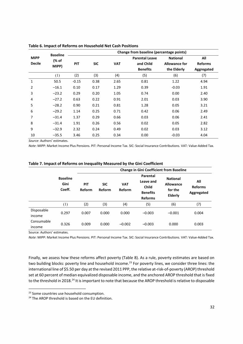
32

Table 6. Impact of Reforms on Household Net Cash Positions

MIPP Decile

Baseline (% of MIPP)

Change from baseline (percentage points)

PIT SIC

VAT

Parental Leave and Child Benefits

National Allowance for

the Elderly

All Reforms

Aggregated (1) (2) (3) (4) (5) (6) (7) 1 50.5 -0.15 0.38 2.65 0.81 1.22 4.94 2 –16.1 0.10 0.17 1.29 0.39 -0.03 1.91 3 –23.2 0.29 0.20 1.05 0.74 0.00 2.40 4 –27.2 0.63 0.22 0.91 2.01 0.03 3.90 5 –28.2 0.90 0.21 0.81 1.28 0.05 3.21 6 –29.2 1.14 0.25 0.71 0.42 0.06 2.49 7 –31.4 1.37 0.29 0.66 0.03 0.06 2.41 8 –31.4 1.91 0.26 0.56 0.02 0.05 2.82 9 –32.9 2.32 0.24 0.49 0.02 0.03 3.12 10 –35.5 3.46 0.25 0.34 0.00 -0.03 4.04

Source: Authors’ estimates. Note: MIPP: Market Income Plus Pensions. PIT: Personal Income Tax. SIC: Social Insurance Contributions. VAT: Value-Added Tax. Table 7. Impact of Reforms on Inequality Measured by the Gini Coefficient

Baseline Gini

Coeff.

Change in Gini Coefficient from Baseline

PIT Reform

SIC Reform

VAT Reform

Parental Leave and

Child Benefits Reforms

National Allowance

for the Elderly

All Reforms

Aggregated

(1) (2) (3) (4) (5) (6) (7) Disposable income

0.297 0.007 0.000 0.000 –0.003 –0.001 0.004

Consumable income

0.326 0.009 0.000 –0.002 –0.003 0.000 0.003

Source: Authors’ estimates. Note: MIPP: Market Income Plus Pensions. PIT: Personal Income Tax. SIC: Social Insurance Contributions. VAT: Value-Added Tax.

Finally, we assess how these reforms affect poverty (Table 8). As a rule, poverty estimates are based on two building blocks: poverty line and household income.23 For poverty lines, we consider three lines: the international line of $5.50 per day at the revised 2011 PPP, the relative at-risk-of-poverty (AROP) threshold set at 60 percent of median equivalized disposable income, and the anchored AROP threshold that is fixed to the threshold in 2018.24 It is important to note that because the AROP threshold is relative to disposable

23 Some countries use household consumption. 24 The AROP threshold is based on the EU definition.

33

income, it can change when household disposable income rises or falls. For this reason, we also consider the anchored AROP threshold in 2018. In other word, this anchored AROP threshold does not move when household disposable income is affected by fiscal policy reforms. The international poverty line ($5.50) is fixed regardless of any change in disposable income. For household income, we examine changes in poverty using both disposable and consumable income, as we did when assessing redistributive effects of reforms. Table 8, column 1 presents pre-reform poverty as seen in section 5.2. Table 8, columns 2–7 show the impact of the reforms.

At the baseline in 2018, poverty rate using household disposable income and the AROP threshold25 is 15.8 percent. This means, prior to fiscal policy reforms, 15.8 percent of the population have their disposable income below the AROP threshold therefore are considered poor. However, baseline poverty rate is 30.6 percent when using consumption income and the AROP threshold. Considering the international poverty line of $5.50 per day at the revised 2011 PPP26, baseline poverty rate is only 2.0 percent and 6.3 percent if using disposable income and consumption income, respectively (Table 8, column 1).

When poverty estimates are based on household disposable income and fixed poverty lines (either the anchored AROP threshold or the international poverty line), all reforms27 have negligible impact on poverty. As shown in Table 6, these reforms provide limited cash gains to people in the first and the second deciles of the income distribution to lift them above the poverty lines.

But when considering household disposable income and relative AROP threshold, the PIT and parental leave and child benefits have noticeable poverty-impacts. The PIT reforms increase national poverty from 15.8 to 16.1 percent (Table 8, column 2). The reason is that the rich benefiting most from PIT reforms raises median disposable income, which pushes up the AROP threshold, and more people now fall below it. Similarly, while reform of parental leave and child benefits provides positive cash flows for households in the lower six deciles of the income distribution, it too increases median disposable income, and thus the AROP threshold. As for the poor, the rise in AROP threshold exceeds the gains from the parental leave and child benefits reform, so the net effect is an increase in national poverty by 0.6 pp (Table 8, column 5). The cumulative effect on poverty of all reforms between 2018 and 2021 would be that an additional 1.3 percent of Croatians become poor (Table 8, column 7).

Poverty-reducing impacts of these reforms – in particular VAT, PIT, and parental leave and child benefits – are more significant if poverty is measured by household consumption income that reflects VAT expenses. Cash benefits from the reduction in VAT rate for food items are higher among people in the lowest 3 income deciles. In fact, VAT reforms contributed to 0.7 percent reduction in poverty when using either the relative or anchored AROP thresholds (Table 8, column 4). The corresponding figure is 0.4 percent reduction when the international poverty line is considered.

25 Equivalent to 84.3 HRK/adult equivalent/day at 2018 prices. 26 Equivalent 24.7 HRK/person/day at 2018 prices. 27 Note that VAT is not captured in household disposable income.

34

Table 8. Impact of Reforms on Poverty

Poverty Baseline

(%)

Change in Poverty from Baseline, Percentage Points

PIT Reform

SIC Reform

VAT Reform

Parental Leave and Child

Benefits Reform

National Allowance for

the Elderly

All Reforms

Aggregated

(1) (2) (3) (4) (5) (6) (7)

Poverty line: 60% of median equivalized disposable income (relative line) Disposable income

15.8 0.3 0.0 0.0 0.6 0.0 1.3

Consumable income

30.6 0.0 -0.1 -0.7 -0.1 -0.1 -0.5

Poverty line: 60% of median equivalized disposable income (anchored to the baseline threshold) Disposable income

15.8 0.0 -0.1 0.0 0.0 0.0 -0.1

Consumable income

30.6 -0.4 -0.2 -0.7 -0.8 -0.1 -1.9

Poverty line: $5.50 PPP a day per person (absolute line) Disposable income

2.0 0.0 0.0 0.0 0.0 -0.1 -0.1

Consumable income

6.3 0.0 0.0 -0.4 -0.1 -0.1 -0.4

Source: Authors’ estimates. Note: MIPP: Market Income Plus Pensions. PIT: Personal Income Tax. SIC: Social Insurance Contributions. VAT: Value-Added Tax.

Meanwhile, PIT and parental leave and child benefits reforms have poverty-reducing effects only when using the anchored AROP threshold and household consumption income. This is because people in the 3rd decile of the income distribution – corresponding to the baseline poverty rate with consumption income and anchored AROP threshold – are less likely to benefit from social programs, so their cash gains from PIT reduction are not affected by potential losses in social benefits. As discussed above, parental leave and child benefits reform lead to net gains for households in the lower half of the income distribution: child benefits reform helps people in the lowest deciles while parental leave benefit for working parents help people in the middle of the income distribution. In net, people in the 3rd income decile are likely to gain from both child benefits and parental leave benefits and are likely to be lifted out of poverty with these reforms.

Box 1: Suggestions for poverty-alleviation policies

Our findings show that it is crucial to understand the interaction among fiscal policies and their distributional impacts. A reduction in PIT rates, for example, could unintentionally lead to net income losses for the poorest because their cash gains from tax reduction can be overshadowed by cash losses from being ineligible to some social benefits due to their higher disposable income. In addition, a PIT reduction without any other accommodating policies can widen the wealth gaps between the rich and the poor in Croatia, as shown in section 7.2 above. Some potential policies aiming to support people at the bottom of the income distribution could include, among others, a reduction in indirect taxes (VAT) for certain goods and services consumed by the poor, and an expansion of social benefits both in terms of coverage and generosity, in particular poverty-targeted

35

programs (guaranteed minimum benefit, compensation for electricity costs, and housing-related benefits), and child benefits. The main poverty-targeted instrument in Croatia is the guaranteed minimum income (GMI) benefits but it has limited poverty-reducing impacts because of its size. In 2018, it covered approximately 80,000 beneficiaries, which was only about 20 percent of the people in the first decile of the income distribution. In other words, only one in every five poorest people benefitted from the GMI program. An option to expand the coverage and the amount of benefits is to increase the GMI base which has been stagnant at 800 HRK/month/eligible person since the day the program was introduced. The GMI base could be increased and indexed (e.g. to inflation, median wage or disposable income) to reflect changes in costs of living for the poorest over time. In addition, some eligibility criteria such as wealth-tests might be relaxed to potentially include more people in the program. Similarly, child benefits – a much bigger program than the GMI program – have the potential to further expand its coverage and generosity to the poorest. In 2018, the program covered approximately 600,000 individuals. About 50 percent of people in the bottom two income deciles benefitted from the program. The amount of child benefits depends on household income which is categorized into 3 brackets – those in the lowest bracket have higher benefits (see Annex A for the exact income brackets and corresponding benefit amounts). An option to target the poorest is to increase household income threshold and amount of benefits for those in the lowest bracket. Finally, for any policy reform, it is equally important to consider its fiscal costs to ensure the program’s sustainability and feasibility. We have developed a CROsimtool to support such policy consideration. This is an Excel-based simulation tool to estimate fiscal costs and distributional impacts of taxes and social benefits reforms. For more information, see Nguyen and Rubil (2021) “CROsimtool instructions for users”.

8 Conclusions and Policy Insights Distributional analysis can be an important tool for a government considering tax or social assistance reform. It sheds light on how fiscal policy affects citizen well-being and enhances the equity lens of its policy intervention. The analysis complements other considerations, such as the budgetary impact and efficiency of revenue collection and spending. The distributional aspect of policies is particularly crucial as the government is aiming to turn the tide on COVID-19 crisis by stimulating a faster economic bounce-back and providing fiscal supports to workers and firms. This resilience and recovery plan needs to benefit people in the lower end of the income distribution.

This paper shows that in 2018 the fiscal system in Croatia contributed to a reduction in inequality but increased poverty. All interventions except indirect taxes had a positive role in reducing inequality, but only direct transfers had poverty-reducing effects, especially for families with three or more children and for retired people. Among direct transfer programs, disability pensions and benefits, child benefits, and guaranteed minimum benefits are the most pro-poor and equalizing. Although direct taxes (PIT and property taxes) apparently have no impact on poverty, indirect taxes (VAT and excises) not only widen the income gap between rich and poor but also increase poverty. The adverse impact of indirect taxes on poverty is so large that it outweighs the poverty-reducing effects of direct transfers.

Compared to other EU countries, Croatia’s performance is about average in terms of the redistributive effects of the fiscal system. Overall, the impact is close to that in Poland.

36

Reforms introduced between 2018 and 2021 helped reduce poverty, measured as the share of population with consumable income lower than one of the three poverty lines considered: the international poverty line at $5.5 a day at the revised 2011 PPP, the relative at-risk-of-poverty threshold, and the anchored at-risk-of-poverty threshold. The poverty-reducing effects come mostly from the reduction of VAT rates on certain food items, and parental leave and child benefits reforms.

However, these reforms, mostly the PIT reforms, contributed to an increase in inequality. A reduction in PIT rates, an increase in the lower limit of the second PIT bracket, and tax relief for young workers led to a net loss for people at the bottom of the income distribution because an increase in disposable income makes some of them ineligible for certain social assistance benefits. Meanwhile, the richer households benefit more from these PIT-related reforms because rates for the top PIT brackets were cut more and the tax on rental and capital income was reduced.

Finally, this analysis highlights the need for a comprehensive understanding of the interaction among fiscal policies and their redistributive and poverty-reducing impacts. A careful assessment of the distributional impacts of policies could mitigate unintended consequences to people in the lower end of the income distribution. Some poverty-alleviation policies could be considered such as a reduction in indirect taxes (VAT) for certain goods and services consumed by the poor, and an expansion of social benefits (e.g. guaranteed minimum income, child benefits) both in terms of coverage and generosity.

37

References Bezeredi, Slavko, and Ivica Urban. 2016. “Predicting Gross Wages of Non-employed Persons in Croatia.”

Financial Theory and Practice 40(1): 1–61.

Bornukova, Kateryna, Gleb Shymanovich, and Alexander Chubrik. 2017. “Fiscal Incidence in Belarus: A Commitment to Equity Analysis.” Policy Research Working Paper 8216, World Bank, Washington, DC.

Chatsiou, Kakia et al. 2020. “Baseline Results from the EU28 EUROMOD: 2016-2019.” EUROMOD Working Paper Series EM 20/20, Brussels: Joint Research Centre of the European Commission.

Cok, Mitja, Ivica Urban, and Miroslav Verbic. 2012. “Income Redistribution through Taxes and Social Benefits: The Case of Slovenia and Croatia.” MPRA Paper No. 38918. https://ideas.repec.org/p/pra/mprapa/38918.html.

Croatian Bureau of Statistics. 2018. Statistical Year Book. https://www.dzs.hr/Hrv_Eng/ljetopis/ 2018/sljh2018.pdf.

Enami, Ali, Nora Claudia Lustig, and Rodrigo Aranda. 2017. “Analytic Foundations: Measuring the Redistributive Impact of Taxes and Transfers.” In Commitment to Equity Handbook. A Guide to Estimating the Impact of Fiscal Policy on Inequality and Poverty, edited by Nora Lustig. Center for Global Development Working Paper No. 446. Washington, DC: Brookings Institution Press and CEQ Institute. SSRN: https://ssrn.com/abstract=2893797.

Eurostat. 2021. General Government Expenditure by Function. https://appsso.eurostat.ec.europa.eu/ nui/show.do?dataset=gov_10a_exp&lang=en.

Foster, J., J. Greer, and E. Thorbecke. 1984. “A Class of Decomposable Poverty Measures. Econometrica 52: 761–66.

Fuchs, Alan and María Fernanda González Icaza. 2021. “Tobacco taxes for improving welfare and distributional outcomes: the case of Georgia.” European Journal of Public Health, 2021.

Gomez Bengoechea, Gonzalo. 2020. "The Welfare State in Spain: An Impact Assessment." Commitment to Equity (CEQ) Working Paper Series 95, Tulane University, New Orleans, LA.

Goraus, Karolina, and Gabriela Inchauste. 2016. “The Distributional Impact of Taxes and Transfers in Poland”. Policy Research Working Paper 7787. World Bank, Washington D.C.

Higgins, Sean, and Nora Lustig. 2016. “Can a Poverty-Reducing and Progressive Tax and Transfer System Hurt the Poor?” Journal of Development Economics 122: 63–75.

Inchauste, Gabriela and Ivica Rubil. 2017. “The Distributional Impact of Taxes and Social Spending in Croatia.” World Bank, Washington, DC.

Inchauste, Gabriela, and Eva Militaru. 2018. “The Distributional Impact of Taxes and Social Spending in Romania.” World Bank, Washington, DC.

Inchauste, Gabriela, and Ivica Rubil. 2017. “The Distributional Impact of Taxes and Social Spending in Croatia.” World Bank, Washington DC.

38

Kakwani, N. 1993. “Statistical Inference in the Measurement of Poverty. Review of Economics and Statistics 75 (4): 632–39.

Lambert, Peter. 2001. The Distribution and Redistribution of Income. 3rd edition. Manchester, UK: Manchester University Press.

Lopez-Calva, Luis F., Nora Lustig, Mikhail Matytsin, and Daria Popova. 2017). “Who Benefits from Fiscal Redistribution in the Russian Federation?” Working Paper 39, CEQ Institute, Tulane University, New Orleans, LA.

Lustig, Nora, editor. 2017. Commitment to Equity Handbook: Estimating the Impact of Fiscal Policy on Inequality and Poverty. Brookings Institution Press, Washington, DC, and CEQ Institute, Tulane University, New Orleans, LA. http://www.commitmentoequity.org/publications/handbook.php.

Madžarević-Šujster, Sanja. 2002. “An Estimate of Tax Evasion in Croatia.” Occasional paper series, Institute of Public Finance, Zagreb 13 (2002): http://www.ijf.hr/OPS/13.pdf

Rossignolo, Dario. 2017. “CEQ Master Workbook: Argentina. Version: May 19, 2017,” CEQ Data Center on Fiscal Redistribution, CEQ Institute, Tulane University, New Orleans, LA.

Scott, John. 2013. “CEQ Master Workbook: Mexico. Version: September 2, 2013.” CEQ Data Center on Fiscal Redistribution, CEQ Institute, Tulane University, New Orleans, LA.

Urban, Ivica, Slavko Bezeredi, and Martina Pezer. 2020. “EUROMOD Country Report: Croatia 2017-2020.” https://www.euromod.ac.uk/sites/default/files/country-reports/year11/ Y11_CR_HR_Final.pdf.

Urban, Ivica. 2016. “Impact of Taxes and Benefits on Inequality among Groups of Income Units.” Review of Income and Wealth 62(1): 120–44.

World Bank, 2021a. Poverty & Equity Brief – Croatia. April 2021. https://databank.worldbank.org/data/download/poverty/987B9C90-CB9F-4D93-AE8C-750588BF00QA/SM2021/Global_POVEQ_HRV.pdf

World Bank, 2021b. “Croatia Public Finance Review.” Forthcoming.

World Bank. 2020. Taxes on Sugar-Sweetened Beverages : Summary of International Evidence and Experiences. World Bank, Washington, DC. © World Bank. https://openknowledge.worldbank.org/handle/10986/33969 License: CC BY 3.0 IGO.

Younger, Stephen D., and Artsvi Khachatryan. 2014. “CEQ Master Workbook: Armenia. Version: May 31, 2014.” CEQ Data Center on Fiscal Redistribution, CEQ Institute, Tulane University, New Orleans, LAm and the World Bank, Washington, DC.

Younger, Stephen, and Dajana Draganic. 2017). “Fiscal Incidence in Montenegro.” World Bank: Washington DC.

39

Annex A. Description of fiscal instruments included in analysis

1. Personal income tax

Liability to tax: All individuals earning income from taxable sources are liable to the PIT.

Taxable income sources: Income from employment; income from self-employment; income from contractual work; pensions (including survivor pensions); rental income; capital income.

Tax allowances: The amount of social insurance contributions paid; personal tax allowance consisting of basic personal allowance and allowance for dependent family members (see table A1)

Table A1. Tax allowances in 2018

Allowance HRK per month Basic personal allowance 3,800 Allowances for dependent family members Adult 1,750 First child 1,750 Second child 2,500 Third child 3,500 n-th child 2,500 × [0.5 + 0.05 × n × (n + 3)] Supplement for each dependent family member with disability Partial disability (< 100%) 1,000 Full disability (100%) 3,750

Basic personal allowance increased to HRK 4,000 as of 2020.

Tax deduction: Donations for cultural, educational, scientific, medical, humanitarian, sports, and religious purposes (maximum per year: 2% of the previous year’s taxable income; contributions to the voluntary pension fund (maximum per year: HRK 6,000); deductions for the self-employed spending on research and development, spending on education of young workers, or employing people from areas of special state concern.

Tax base: The general tax base, applied for taxation of employment income, self-employment income, and pensions equals income net of social insurance contributions, minus total tax deductions and total tax allowances. In the case of income from contractual work, the base equals gross income minus pension contributions. In the case of capital income, the base equals gross income. In the case of rental income, the base equals 70% of gross income.

Tax rates/amounts: The tax rates applied for taxation of employment income, self-employment income, and pensions are defined by a general schedule shown in table A2. This is the monthly general schedule; the yearly schedule is obtained by multiplying the tax base by 12. The schedules for 2019 and 2021 are shown in tables A3 and A4. There are also a number of income source-specific tax rates (table A5). Self-employed farmers with an annual revenue up to HRK 300,000 pay the tax as lump-sum (in the sense: independent from gross income), depending on annual revenue, as shown in table A6.

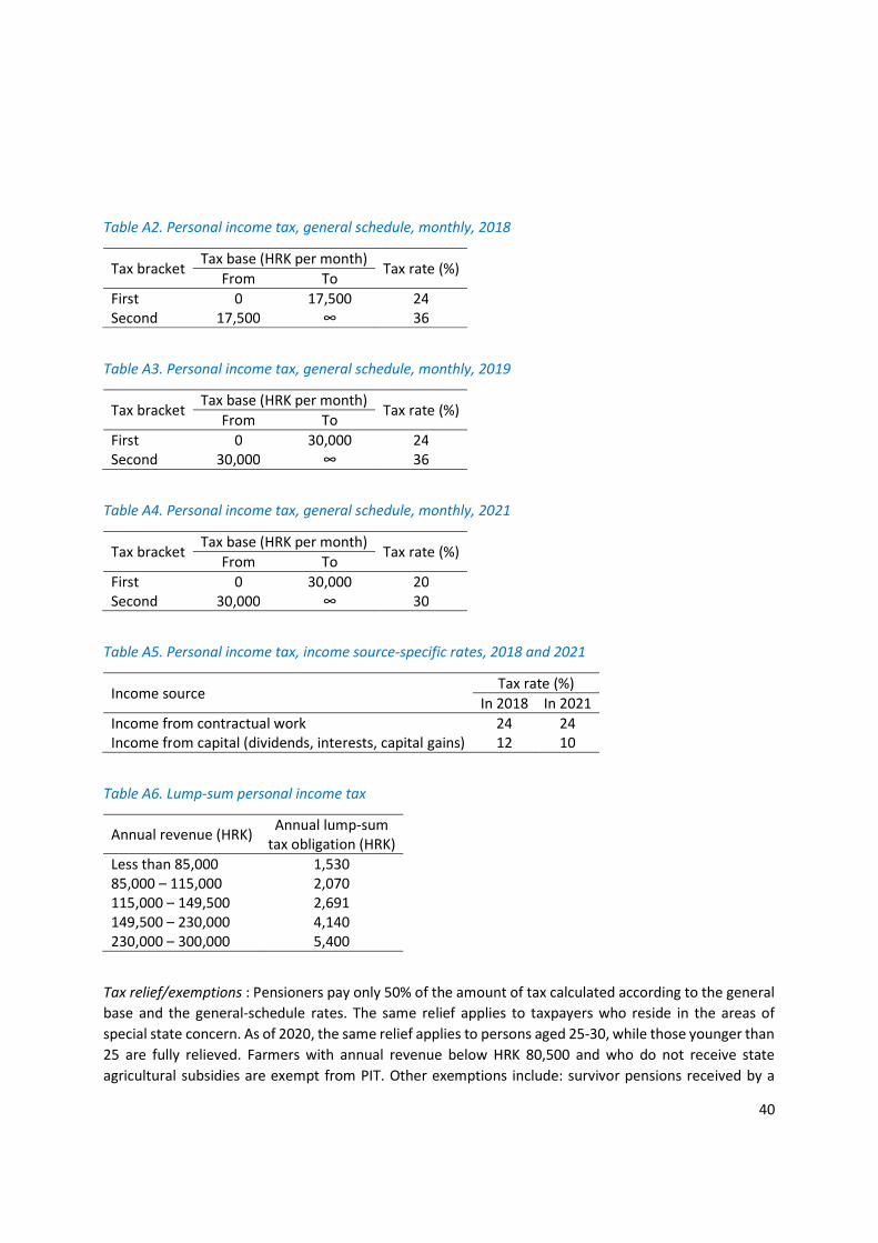
40

Table A2. Personal income tax, general schedule, monthly, 2018

Tax bracket Tax base (HRK per month) Tax rate (%) From To First 0 17,500 24 Second 17,500 ∞ 36





Table A5. Personal income tax, income source-specific rates, 2018 and 2021

Income source Tax rate (%) In 2018 In 2021

Income from contractual work 24 24 Income from capital (dividends, interests, capital gains) 12 10

Table A6. Lump-sum personal income tax

Annual revenue (HRK) Annual lump-sum tax obligation (HRK)

Less than 85,000 1,530 85,000 – 115,000 2,070 115,000 – 149,500 2,691 149,500 – 230,000 4,140 230,000 – 300,000 5,400

Tax relief/exemptions : Pensioners pay only 50% of the amount of tax calculated according to the general base and the general-schedule rates. The same relief applies to taxpayers who reside in the areas of special state concern. As of 2020, the same relief applies to persons aged 25-30, while those younger than 25 are fully relieved. Farmers with annual revenue below HRK 80,500 and who do not receive state agricultural subsidies are exempt from PIT. Other exemptions include: survivor pensions received by a

41

child younger than 15 at the moment the parent passed away; survivor pensions received by persons younger than 18; survivor pensions received by persons younger than 26 and in regular education.

Modeling notes: There is no sufficient information in the SILC to differentiate between the following three groups of self-employed farmers: those paying PIT according to the general schedule; those paying PIT as lump-sum; those exempt from PIT. We therefore assume that 75% of them are exempt from PIT, while the rest are those paying PIT according to the general schedule. Thus, each farmer has a 25-percent chance of paying PIT, and this probability is considered in the calculation of the final PIT obligation. Moreover, there is also insufficient information in the SILC to identify persons earning income from contractual work. Thus, we cannot apply the rate specific to this income source. Assuming that people earning this type of income reported it as income from self-employment, their PIT obligation is calculated as the PIT paid on self-employment income.

2. Surtax

Liability to tax: Every payer of personal income tax is liable to surtax as well.

Tax base: The base equals the personal income tax obligation.

Tax rates: Every local government sets the rate applicable to its residents. There are restrictions regarding the maximum rate. The allowed maximum rates are: 10% for municipalities; 12% for towns less than 30,000 inhabitants; 15% for towns with more than 30,000 inhabitants. An exception to the rule is Zagreb, the capital, where the maximum rate is set to 30%, and the current rate is 18%.

Modeling notes: The SILC does not provide information about the municipality/town of residence. Therefore, we cannot model surtax by applying the exact rates. Instead, we calculate the population-weighted average surtax rate across all towns/municipalities. This gives us a single rate of 9.42 percent which we apply to every household in the sample. Weighting by the working population rather than total population matters very little.

Employer social insurance contributions

Types of contributions: General health contribution, occupational health contribution, and employment contribution.

Liability to contributions: In principle, the contributions must be paid by every employer for each employee.

Relief/exemptions: Employers do not have to pay the contributions for workers satisfying either of the following criteria: workers employed for the first time (maximum duration of relief: 1 year); workers employed after being long-term unemployed (maximum duration of relief: 2 years); workers employed after being unemployed who have less than one year of work experience (maximum duration of relief: 2 years); workers who signed a permanent contract with the employer before the age of 30 (maximum duration: 5 years).

Contribution base: The base equals gross income from employment. The base floor is 38% of the national average gross wage from January to August of the previous year. There is no base ceiling.

Contribution rates: 15% for the general health contribution; 1.7% for the occupational health contribution; 0.5% for the employment contribution. As of 2019, the general health contribution rate increased to

42

16.5%, whereas the rates for employment and occupational health contributions fell to zero (i.e., the contributions were abolished).

3. Employee social insurance contributions

Types of contributions: Pension contribution.

Liability to contributions: Every employee earning employment income must pay the contributions.

Contribution schemes: There are two schemes. Scheme A is a pension scheme fully based on mandatory generational solidarity (pillar 1). Scheme B is a pension scheme consisting of two parts: one part is based on generational solidarity (pillar 1), the other on mandatory capitalized savings (pillar 2). Persons who were younger than 40 in 2002, when the pension reform took place, were automatically assigned to scheme B. Persons older than 50 were automatically assigned to scheme A. Persons aged between 40 and 50 could choose the scheme.

Contribution base: The base equals gross income from employment. The base floor is 38 percent of the national average gross wage from January to August of the previous year. For pillar 1 in both scheme A and scheme B, the monthly (yearly) ceiling base is 6 (72) times the national average gross wage from January to August of the previous year. For pillar 2 in scheme B there is no ceiling base.

Contribution rates: For scheme A, the rate is 20%. For scheme B, the rates are 15% and 5% for pillars 1 and 2, respectively.

4. Self-employed social insurance contributions

Types of contributions: General health contribution, occupational health contribution, employment contribution, and pension contributions.

Liability to contributions: Every self-employed person must pay the contributions on his/her income.

Contribution base: The base is the product of the national average gross wage from January to August of the previous year and a factor depending on type of self-employment. The factors are shown in table A7.

Contribution rates: The rates are given in table A8.

Modeling notes: The only information in the SILC on type of self-employment is whether a self-employed person is a farmer or a non-farmer. Thus, we cannot simulate these contributions considering the different factors across types of unemployment shown in table A7. Thus, for all self-employed non-farmers, we assume that the relevant factor is 0.65, which applies to craftsmen and some other types (see table A7). We do so because craftsmanship is the most common type of self-employment in Croatia.

Moreover, we do not have sufficient information to classify farmers into the three groups from table A7. Therefore, we assume that 75% of all self-employed farmers are exempt from PIT, while all the remaining 25% are those paying PIT according to the general schedule. This is equivalent to assuming that each farmer has a 75-percent chance of being the former type, and a 25-percent chance of being the latter type. Each farmer’s contributions are then obtained as a random variable respecting these chances.

43

Table A7. Factors for determination of contribution base for different types of self-employment

Type of self-employment Factor Health workers, veterinarians, lawyers, notaries, auditors, engineers, architects, tax advisors, bankruptcy trustees, interpreters, translators, tourism workers

1.1

Craftsmen, nurses, dental technicians, physiotherapists, movie workers, journalists 0.65 Farmers paying personal income tax according to general schedule 0.55 Farmers paying personal income tax as lump-sum 0.40 Farmers exempt from personal income tax 0.35

Table A8. Self-employment contribution rates

Type of contribution Contribution rate (%)

Farmers exempt from personal income tax

Other types of self-employment

General health 7.5 15 Occupational health 0.5 0.5 Employment 1.7 1.7 Pension, scheme A 10 20 Pension, scheme B, pillar 1 5 15 Pension, scheme B, pillar 2 5 5

5. Social insurance contributions on income from contractual work

Types of contributions: General health contribution and pension contributions.

Liability to contributions: All individuals earning income from contractual work must pay the contributions.

Contribution base: The base is equal to gross receipt from contractual work. The base amount is not restricted by a floor or ceiling. If a receipt from contractual work is honoraria for scientists’ or journalists’ original work, the base equals 70% of gross receipt, while in the case of artists’ honoraria, the base equals 45% of gross receipt.

Contribution rates: The rates are: 7.5% for the general health contribution; 10% for the pension contribution in scheme A; 7.5% for the pension contribution to pillar 1 in scheme B; 2.5% for the pension contribution to pillar 2 in scheme B.

Modeling notes: Since there is no information on income from contractual work in the SILC, we cannot compute these contributions. We assume that income from contractual work is reported as self-employment income and calculate the contributions for people earning income from contractual income as if they were self-employed.

6. Pensioners’ health contribution

Type of contributions: General health contribution.

Liability to contributions: Every person receiving public pension.

Contribution base: The base is equal to gross pension.

44

Contribution rates: The rate is 3% if gross pension is above the national average net wage from January to August of the previous year. Otherwise, the rate is 1%, and the contribution is paid by government (see below under credited contributions).

7. Credited social insurance contributions

Credited contributions are those paid by government for certain population groups. The eligible groups, types of contributions, contribution base, and contribution rates are given in table A9.

Table A9. Credited social insurance contributions

Eligible group Type of contributions Contribution base Contribution rate

Persons on maternity or parental leave

Pension contribution to pillar 2 in scheme B 35% of NAGW 5%

Unemployed persons Pension contribution to pillar 2 in scheme B 35% of NAGW 5%

Unemployed persons General health contribution 35% of NAGW 5%

Pensioners with gross pension below NANW

General health contribution Gross pension 1%

Persons on sick leave Pension contribution to pillar 2 in scheme

Amount of sickness benefit 5%

Notes: NAGW (NANW) – national average gross (net) wage from January to August of the previous year.

As of April 2020, the eligibility extended to recipients of the Covid-19 wage compensation. For them, government pays the pension contribution to pillar 2 in scheme B. The contribution base equals the mount of Covid-19 wage compensation divided by 0.8, and the contribution rate is 5%.

8. Old-age pension

Eligibility:

Regular old-age pension: Eligible is every man (woman) who retired at the statutory retirement age of 65 (62) and spent at least 15 years working, that is, paying contributions for pension insurance. As of 2030, the statutory retirement age for women and men will be the same; this will be achieved through gradual increase in the statuary retirement age for women.

Early old-age pension: Eligible is every man (woman) who retired at most five years before the statutory age of 65 (62) and spent at least 35 years (32 years and six months) working, that is, paying contributions for pension insurance. As of 2030, the minimum length of the contributory history for men and women will be the same; this will be achieved through gradual increase in the minimum for women.

Means-testing: Neither regular nor early old-age pension is means-tested.

Benefit amount: In general, the amount of old-age pension received depends on the history of contributions for pension insurance. Pensioners who contributed to the pension scheme A, that is, those who contributed to pillar 1 (generational solidarity) only, receive their pensions from this pillar. Those who contributed to pension scheme B, that is, those who contributed to both pillar 1 and pillar 2 (capitalized savings), receive their pensions from both pillars. See the description of pension contributions

45

above. In the case of early old-age pension, there is a penalty of 0.3% per month of the gap between the actual and the statutory retirement age.

Modeling notes: Old-age pension is not simulated, as the required information is not available in the SILC. Rather, we directly take the amounts reported by respondents. The SILC does not allow distinguishing between regular and early old-age pensions, but the distinction is not relevant to our analysis anyways. Moreover, we have no information to distinguish between pensions from pillar 1 and pillar 2; this distinction is not relevant for the analysis either.

9. Guaranteed minimum benefit

Eligibility: An eligible person must satisfy either of the following conditions:

younger than 15; aged 15-29 and in regular education; older than 65; older than statutory retirement age minus 5 years; unemployed; unable to work; pregnant; caring for a child younger than 1; caring for twins younger than 3; caring for three children younger than 10; caring for a person with disability.

Means-testing: The benefit is both income- and wealth tested.

Income test: For a household to pass the income test, total household income must be below the ‘means of subsistence’ (to be defined shortly). The income concept used for the income-test includes income from all sources taxable by personal income tax, net of personal income tax and social insurance contributions. Alimonies paid are deducted, and alimonies received are added (only the portion exceeding 8.5%, 10%, and 11% for each dependent child aged 0-6, 7-12, and 13-18, respectively). The maternity leave benefit, parental leave benefit, maternity and parental allowance, sickness benefit, unemployment benefit are also deducted. The “means of subsistence” is equal to the sum of the respective contributions of each eligible household member. The contributions vary by household type and member type, as shown in table A10. For example, for a lone parent, able to work, with two children, one aged 10, the other aged 20 and studying at a university, the means of subsistence equal to HRK 800 + 440 + 440 = HRK 1,680.

Wealth test : For a household to pass the wealth test, it must satisfy the following conditions: o it must not possess a car, except if the household is large (6 or more members), or the car is

used for transport of a household member with disability, or the residence is far from a town and there is no public transport;

o it must not possess more than one house/apartment; o it must not possess any property that can be used, but it is not used, to satisfy basic needs.

46

Table A10. Contributions to ‘means of subsistence’

Household and member type Contribution to

‘means of subsistence’ (HRK per month)

Single person Able to work 800 Unable to work 920 Adult in household with multiple members Able to work 480 Unable to work 480 Lone parent (the other parent is unknown or dead, not just absent from the household) Able to work 800 Unable to work 800 Child in non-lone-parent household (including one-parent households where the other parent is known and alive) Aged 0-6 320 Aged 7-14 320 Aged 15-17 320 Aged 18-29 and in regular education 480 Child in lone-parent household Aged 0-6 440 Aged 7-14 440 Aged 15-17 440 Aged 18-29 and in regular education 480

Benefit amount: The benefit amount equals the amount by which total household income falls short of the means of subsistence.

Other design features: There is a ‘make-work-pay’ element in-built. A person able to work, who receives the benefit for longer than a year, will not lose the whole amount of benefit the moment (s)he gets employed. Instead, the benefit is phased out gradually. In the first month of employment, the benefit remains the same as before employment; in the second month, the benefit is reduced by 25% relative to the amount before employment; in the third month, the benefit is reduced by 50% relative to the amount before employment. For further months, provided the person stays employed, the benefit is recalculated every three months, considering the average income of the household over the three months preceding the recalculation.

Modeling notes: The SILC data does not allow us to distinguish between ‘single parents’ (the other parent is known and alive) and ‘lone parents’ (the other parent is unknown or dead). For all one-parent households, we assume the parent is a single parent.

47

The SILC data allow us to simulate the wealth test only with respect to car possession. We have sufficient information to model the exceptions as well, as we can identify household size, whether there is a member with disability, and whether the residence is far from a town and public transport is not available. The latter exception is modeled by assuming that the condition of living far from a city and without access to public transportation is well approximated by the condition of living in an area with very low population density. For lack of information in the SILC, we cannot simulate the ‘make-work-pay’ element of the benefit. We do not consider the possibility of benefit non-take-up.

10. Compensation for electricity costs

Eligibility: Eligible is every household receiving the guaranteed minimum benefit, and every household with at least one member receiving the personal disability allowance.

Means-testing: The benefit is income- and wealth-tested indirectly through the income- and wealth-test of the guaranteed minimum benefit, or the income-test of the personal disability allowance.

Benefit amount: The benefit amount equals the monthly cost of electricity but may not exceed HRK 200.

Modeling notes: Since we cannot identify in the SILC data who receives the personal disability allowance, nor do we have information to simulate it, we do not simulate the eligibility condition related to it. We assume the only eligible households are those receiving the guaranteed minimum benefit. Moreover, we assume that eligible household receives the maximum amount.

11. Maternity leave benefit

Eligibility: Eligible are employed or self-employed mothers, during the maternity leave period.

Duration: It starts 28 days before the delivery is due (or, in case of complications with pregnancy, 45 days before the delivery is due), and end 70 days after the delivery.

Means-testing: The benefit is not means-tested.

Benefit amount: The benefit amount is expressed as a percentage of a benefit base. For employed beneficiaries, the benefit base equals gross income minus employee’s contributions, personal income tax and surtax. For self-employed beneficiaries, the benefit base is calculated in the same way, ‘pretending’ that they are employees rather than self-employed. To receive 100% of the benefit base, a beneficiary must be insured either at least 12 months without interruption before the maternity leave, or at least 18 months during the 24 months before the maternity leave in case of interruptions. If this condition is not satisfied, the benefit amounts to a minimum set to 70% of the benefit base (HRK 3,328.20).

Modeling notes: Due to insufficient information in the SILC, we do not know if a mother satisfies the insurance criterion. We assume they all do. To determine exactly the period of the maternity leave, information on the month of birth is required, but is not given in the SILC. Instead, the quarter of birth is provided. For a child born in the first/second/third/fourth quarter, we assume it was born in February/May/August/November, respectively.

12. Parental leave benefit

Eligibility: Eligible are employed or self-employed parents taking care of small children.

48

Duration: The benefit can be claimed for a certain number of months after the period of maternity leave. If the child is the 1st or 2nd, the benefit can be claimed for 6 months if used by the mother only, or for 8 months if it is used by both parents (4 months each). If the child is the 3rd, 4th, etc., or if twins or multiples were born, the benefit can be claimed for 30 months, and used either by the mother alone, or by both parents equally.


Benefit amount: The benefit amount is expressed as a percentage of a benefit base. The benefit base is equal to the eligible person’s average net income over the six months before the parental leave starts. For the first 6 months (or 8 moths if both parents use the benefit equally) of the leave, the benefit amount 100% of the benefit base. It cannot fall below a minimum of HRK 2,328.20 per month, nor can it exceed a maximum of HRK 3,991.20 per month. In the remaining 24 months (or 22 months if both parents use the benefit equally), the benefit amount is HRK 2,328.20 per month. The later amount increased to HRK 5,654.20 as of 2020.

Modeling notes: Of all beneficiaries, less than 3% are fathers (Urban, Bezeredi, and Pezer 2020). In accordance with this, we assume that all beneficiaries are mothers. We also assume that every beneficiary claims the benefit for as long as possible. To determine exactly the period of the parental leave, information on the month of the child’s birth is required, but is not given in the SILC. Instead, the quarter of birth is provided. For a child born in the first/second/third/fourth quarter, we assume it was born in February/May/August/November, respectively.

13. Maternity and parental allowance

Eligibility: Parents of newborn children who are not employed or self-employed (and thus are not eligible for the maternity leave benefit and the parental leave benefit), but rather work only occasionally (e.g., seasonal workers in tourism or agriculture) or do not work (e.g., unemployed, inactive).

Duration: If the child is the 1st or 2nd, the benefit can be claimed for 12 months since the child’s birth. If the child is the 3rd, 4th, etc., or if twins or multiples were born, the benefit can be claimed for 36 months.


Benefit amount: The benefit amount equals HRK 2,328.20 per month.

Modeling notes: Since in the case of parental leave benefit less than 3% are fathers (Urban, Bezeredi, and Pezer 2020), it is very likely that in this holds in the case of maternity and parental allowance. Thus, as in the case of parental leave benefit, we assume that all beneficiaries are mothers. We also assume that every beneficiary claims the benefit for as long as possible.

To determine exactly the duration, information on the month of the child’s birth is required, but is not given in the SILC. Instead, the quarter of birth is provided. For a child born in the first/second/third/fourth quarter, we assume it was born in February/May/August/November, respectively.

14. Grant for newborn child

Eligibility: Eligible are all households with a newborn child.


49

Benefit amount: The benefit amount equals HRK 2,328 per newborn child. This is a one-off benefit, received just once for each newborn child.

15. Child benefit

Eligibility: Eligible are households with dependent children.

Means-testing: The benefit is income-tested. For a household to pass the income test, the monthly income per member must be below HRK 1,663. The income concept used for the test includes income from all sources taxable by personal income tax, net of personal income tax and social insurance contributions. This means that social benefits that are not taxable by personal income tax are not included in this income concept.

Benefit amount: The benefit amount depends on household’s income per member, where ‘income’ refers to the income concept used for the income test. There are three income brackets, each with a bracket-specific amount of benefit, as shown in table A11. In certain cases, the benefit amounts from the table are larger: by 25% (15%) larger if both (one) parent(s) are (is) missing or permanently unable to work and live independently; by 25% for a child with health issues. Top-ups are available for households with three or more dependent children: the total monthly amount of child benefit a household receives is increased by HRK 500 (HRK 1,000) when there are three (four or more) dependent children. In certain cases, the benefit amount does not depend on the household income per member: for a child with disability, the benefit is HRK 831.50 per month; for a child of a killed, captured or missing participant of the Homeland War, the benefit is HRK 374.18 per month.

Table A11. Amounts of child benefits across income brackets

Bracket Household income

per member defining the bracket (HRK per month)

Amount of benefit per child (HRK per month)

1 Less than 543.14 299.34 2 543.15 – 1,119.53 249.45 3 1,119.54 – 1,663 199.56

Modeling notes : Children of killed, captured, or missing participants of the Homeland War cannot be identified in the SILC, and thus we cannot model the higher benefit for them. When parents identify themselves in the SILC as unable to work, we take this as equivalent to the condition that they are ‘permanently unable to work and live independently’.

Unemployment benefit

Eligibility: Eligible are unemployed persons who became unemployed after being employed or self-employed, provided certain conditions are met. For those becoming unemployed after being employed, they must satisfy the condition of having been employed for at least 9 months during the 24 months preceding the start of the current unemployment spell. In addition, unemployment must not be due to a voluntary decision or violation of the work contract. For those entering unemployment from self-employment, there are various cases in which the benefit can be claimed, a typical one being bankruptcy or insolvency.

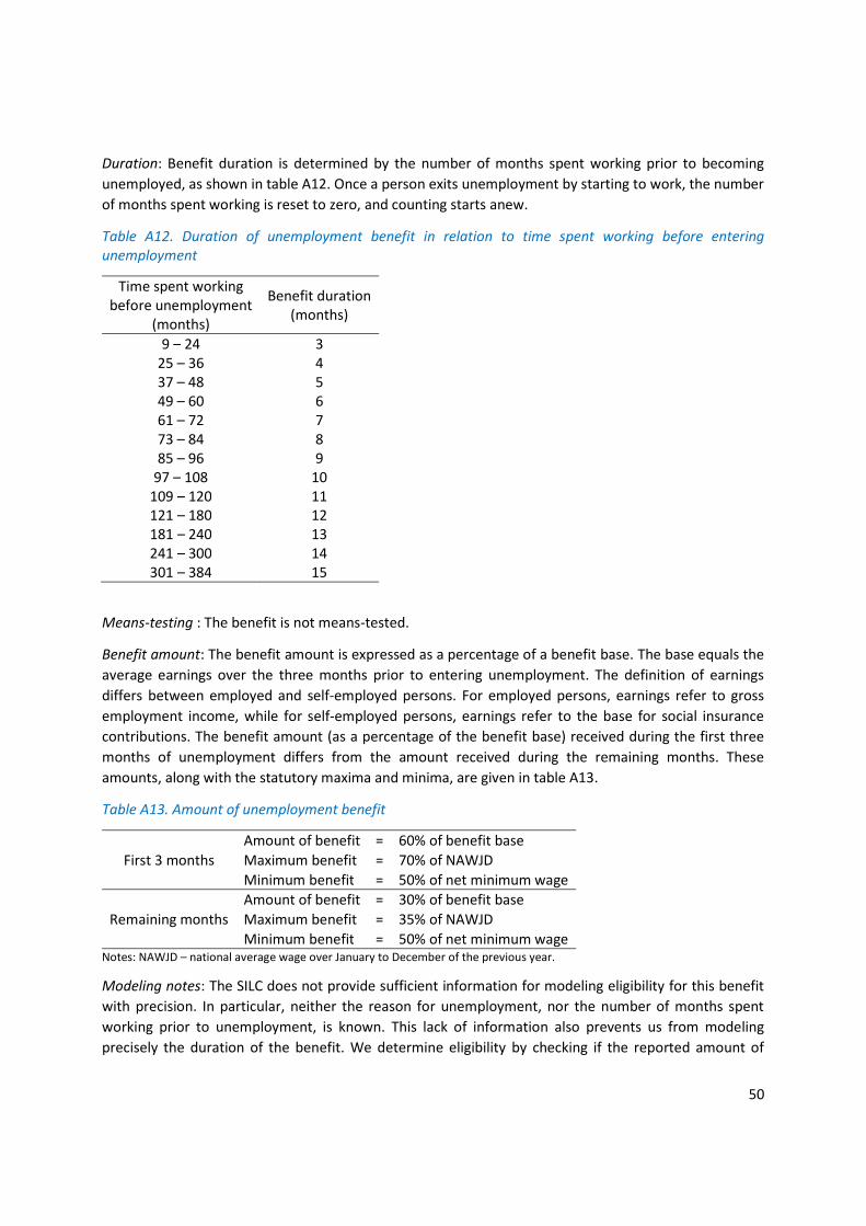
50

Duration: Benefit duration is determined by the number of months spent working prior to becoming unemployed, as shown in table A12. Once a person exits unemployment by starting to work, the number of months spent working is reset to zero, and counting starts anew.

Table A12. Duration of unemployment benefit in relation to time spent working before entering unemployment

Time spent working before unemployment

(months)

Benefit duration (months)

9 – 24 3 25 – 36 4 37 – 48 5 49 – 60 6 61 – 72 7 73 – 84 8 85 – 96 9

97 – 108 10 109 – 120 11 121 – 180 12 181 – 240 13 241 – 300 14 301 – 384 15

Means-testing : The benefit is not means-tested.

Benefit amount: The benefit amount is expressed as a percentage of a benefit base. The base equals the average earnings over the three months prior to entering unemployment. The definition of earnings differs between employed and self-employed persons. For employed persons, earnings refer to gross employment income, while for self-employed persons, earnings refer to the base for social insurance contributions. The benefit amount (as a percentage of the benefit base) received during the first three months of unemployment differs from the amount received during the remaining months. These amounts, along with the statutory maxima and minima, are given in table A13.

Table A13. Amount of unemployment benefit

First 3 months Amount of benefit = 60% of benefit base Maximum benefit = 70% of NAWJD Minimum benefit = 50% of net minimum wage

Remaining months Amount of benefit = 30% of benefit base Maximum benefit = 35% of NAWJD Minimum benefit = 50% of net minimum wage

Notes: NAWJD – national average wage over January to December of the previous year.

Modeling notes: The SILC does not provide sufficient information for modeling eligibility for this benefit with precision. In particular, neither the reason for unemployment, nor the number of months spent working prior to unemployment, is known. This lack of information also prevents us from modeling precisely the duration of the benefit. We determine eligibility by checking if the reported amount of

51

unemployment-related benefits is non-zero; if so, we consider the person as obviously eligible for the benefit. To determine the amount of benefit, we assume for every unemployment person that his/her unemployment spell stared in the year to which the SILC data refer (2018). Finally, we simply apply the rules from table A13.

16. Survivor’s pension

Eligibility:

the widow(er) of a deceased pension-insured person (DPIP), aged 50 or more; the widow(er) of a DPIP, aged below 50, if unable to work or caring for dependent children a child of a DPIS, if aged below 26 and enrolled in secondary or tertiary education (the age limit

does not apply if the child is not able to work).

Duration: The benefit is received for as long as the eligibility conditions are satisfied.


Benefit amount: The benefit amount is the product of a base and the last pension of the DPIP. The base varies with the number of survivors, from 0.7 if there is one survivor to 1 if there are four or more survivors. If the DPIP was not retired at the moment of death, the base is multiplied by the counterfactual disability pension (s)he would receive had (s)he retired due to disability rather than died. Some special rules apply when the DPIP was a participant of the Homeland War or the World War 2.

Modeling notes: We do not simulate this benefit, but rather take the amounts as reported in the SILC. In fact, the survivor’s pension is reported together with other survivor’s benefits, and thus in the analysis we do not consider it as a benefit on its own, but rather as part of a group labeled “survivor’s pension and benefits”. The benefits include mostly those related to cases where the DPIP was a participant of the Homeland War or the World War 2.

17. Disability pension

Eligibility: Eligible are persons who lost the ability to work, fully or partially, and worked certain age-specific minimum number of years.

Duration: The benefit is received for as long as the eligibility conditions are satisfied.

Benefit amount: The amount of benefit is determined in the same way as in the case of old-age pension, as if the eligible person had retired rather than lost the ability to work, but with the years of service being increased by a certain factor specific to the degree of disability.

Modeling notes: We do not simulate this benefit, but rather take the amounts as reported in the SILC. In fact, the disability pension is reported together with other disability benefits, and thus in the analysis we do not consider it as a benefit on its own, but rather as part of a group labeled “disability pension and benefits”. The benefits besides the disability pension are numerous, and here we just list them:

supplement for assistance and care; personal disability allowance; pre-employment supplement; compensation for caregiver;

52

supplement for part-time employed caregiver of child in need of special care; compensation for caregiver of child with severe disability; supplement for part-time employed caregiver of child with severe disability; wage compensation during professional rehabilitation; supplement for physical impairment due to work-related injuries and occupational disease; cash compensation for workers exposed to asbestos; supplement for professional rehabilitation of Homeland War participants with disability.

18. Sickness benefit

Eligibility: In principle, eligible are health-insured employed and self-employed persons, as well as temporary workers, during a sick-leave. A person is considered health-insured if (s)he has been insured before a sick-leave: at least 9 months without interruptions, or at least 12 months with interruptions during the last 24 months. Non-insured persons may receive the benefit nevertheless, but a very small amount.

Duration: The benefit is received during the whole a sick-leave.

Benefit amount: The benefit amount is expressed as a percentage of a benefit base. For employed persons, the benefit base is equal to the average gross income net of personal income tax and surtax over the six months prior to sick-leave. The benefit base for self-employed persons is equal to their base for social insurance contributions. For the first 42 days of a sick-leave, the benefit is financed by the employer, and by government for the rest of sick-leave. The benefit amount may not be lower than 70% of the benefit base. The monthly floor is set to HRK 831.50 and the ceiling to HRK 4,257.28. In certain cases (e.g., pregnancy complications, organ transplantations, occupational diseases, health consequences of participation in the Homeland War, etc.), the benefit amount may not be lower than 100% of the benefit base. These amounts apply for persons satisfying the insurance condition (see under eligibility), and if the condition is not met, the benefit equals the monthly floor of HRK 831.50.

Modeling notes: Due to lack of information in the SILC, we do not simulate this benefit, but rather take the amounts reported by respondents. In particular, there is no information about the number of months spent on sick-leave. Moreover, we do not have information to determine whether a person meets the insurance condition of eligibility, nor can we identify the reason for sick-leave, and without these pieces of information, we cannot simulate the benefit amount.

19. Education-related benefits

This is a group of unidentified benefits, paid by governments at all levels (central, regional, local). They may include benefits conditional on the living standard of the beneficiary’s household, but also benefits based on performance. They may be regular or occasional.

20. Housing-related benefits

This a group of benefits paid mostly by local and regional governments. They are typically means-tested. One example is the compensation for housing costs, whose purpose is to help the needy to pay utility bills (electricity, gas, water). Eligible are beneficiaries of the guaranteed minimum benefit. The amount depends on the costs, and may not exceed half the ‘means of subsistence’ (see the description of the guaranteed minimum benefit above). We assume that this benefit is the main benefit included in the

53

category that we consider, labeled “housing-related benefits”. These benefits are not simulated, but rather taken as reported in the SILC, as a group.

21. VAT

Standard rate: 25%.

Reduced rates: There are two reduced rates, 5% and 13%.

The 5% rate applies to:

bread (does not include other bakery products) milk (does not include other dairy products) books with professional, scientific, artistic, cultural, and educational content medical drugs listed by the Croatian Health Insurance Fund (HZZO) medical equipment, appliances, and disability-related devices listed by the Croatian Health

Insurance Fund (HZZO) cinema tickets daily newspapers scientific journals

The 13% rate applies to:

accommodation with accompanying meals magazines edible oils and fats baby car seats, diapers, and food (other than replacements for mother’s milk) water supply concert tickets electricity supply refuse collection urns and coffins seedlings and plantlets fertilizers, pesticides, and other agrochemical products animal food other than pet food live domestic animals authorship rights of artists

As of 2019, the 13% rate extended to:

fresh meat fresh fish fresh seafood fresh and dried fruit, including all sorts of nuts fresh vegetables eggs of domestic fowl in shell

54

Exemptions: Exempted from the VAT are:

health care services education postal services insurance banking and other financial services social care services

Modeling notes: The HBS does not allow us to simulate the reduced VAT on

medical equipment, appliances, and disability-related devices listed by the Croatian Health Insurance Fund (HZZO)

scientific journals urns and coffins seedlings and plantlets fertilizers, pesticides, and other agrochemical products animal food other than pet food live domestic animals authorship rights of artists

The following assumptions are made:

since expenditures on tickets for cinema, concerts, and theatre are reported as one item, to be able to apply the 13% rate on concert tickets and the 5% rate for cinema ticket, we assume that that one third of the total expenditure on cinema, concerts and theatre is spent on each of them

we assume that all expenditures on medical drugs are on drugs listed by the HZZO

22. Excises

Excises are shown in table A14.

There are also excises on:

cars, which depend on the fuel they use, the engine power, and CO2 emissions vessels airplanes luxury products

Modeling notes : We simulate all excises in table D13. Due to lack of information in the HBS, we do not simulate the excises on cars, vessels, airplanes, and luxury products.

55

Table A14. Excises

Product Excise Cigarettes (specific excise) HRK 310 / 1,000 cigarettes Cigarettes (ad valorem excise) 34% of retail price Cigars HRK 600 / 1,000 cigars Cigarillos HRK 600 / 1,000 cigarillos Finely cut tobacco HRK 600 / kg Other tobacco for smoking HRK 600 / kg Petrol HRK 3,151 / 1,000 L Diesel HRK 2,450.50 / 1,000 L Natural gas HRK 8.10/MWh Liquified natural gas HRK 100 / 1,000 kg Electricity HRK 7.50 / MWh Beer HRK 40 / 1% alcohol volume in 1 hL of beer Ethyl alcohol HRK 5,300 / hL Roasted coffee HRK 6 / kg Coffee extracts, essences, and concentrates HRK 20 / kg Bottled water and non-fruit soft drinks HRK 40 / hL Powders and granules for non-alcoholic beverages HRK 240 / hL

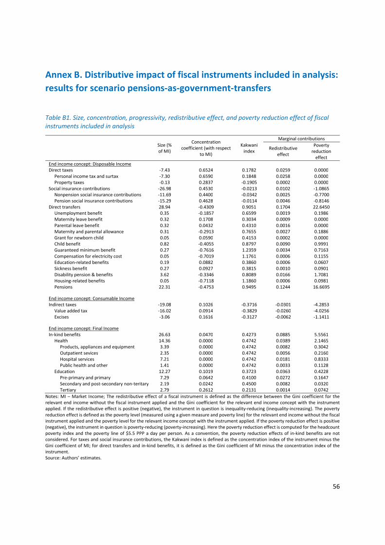
56

Annex B. Distributive impact of fiscal instruments included in analysis: results for scenario pensions-as-government-transfers

Table B1. Size, concentration, progressivity, redistributive effect, and poverty reduction effect of fiscal instruments included in analysis

Size (% of MI)

Concentration coefficient (with respect

to MI)

Kakwani index

Marginal contributions

Redistributive effect

Poverty reduction

effect End income concept: Disposable Income Direct taxes -7.43 0.6524 0.1782 0.0259 0.0000 Personal income tax and surtax -7.30 0.6590 0.1848 0.0258 0.0000 Property taxes -0.13 0.2837 -0.1905 0.0002 0.0000 Social insurance contributions -26.98 0.4530 -0.0213 0.0102 -1.0865 Nonpension social insurance contributions -11.69 0.4400 -0.0342 0.0025 -0.7700 Pension social insurance contributions -15.29 0.4628 -0.0114 0.0046 -0.8146 Direct transfers 28.94 -0.4309 0.9051 0.1704 22.6450 Unemployment benefit 0.35 -0.1857 0.6599 0.0019 0.1986 Maternity leave benefit 0.32 0.1708 0.3034 0.0009 0.0000 Parental leave benefit 0.32 0.0432 0.4310 0.0016 0.0000 Maternity and parental allowance 0.31 -0.2913 0.7655 0.0027 0.1886 Grant for newborn child 0.05 0.0590 0.4153 0.0002 0.0000 Child benefit 0.82 -0.4055 0.8797 0.0090 0.9991 Guaranteed minimum benefit 0.27 -0.7616 1.2359 0.0034 0.7163 Compensation for electricity cost 0.05 -0.7019 1.1761 0.0006 0.1155 Education-related benefits 0.19 0.0882 0.3860 0.0006 0.0607 Sickness benefit 0.27 0.0927 0.3815 0.0010 0.0901 Disability pension & benefits 3.62 -0.3346 0.8089 0.0166 1.7081 Housing-related benefits 0.05 -0.7118 1.1860 0.0006 0.0981 Pensions 22.31 -0.4753 0.9495 0.1244 16.6695

End income concept: Consumable Income Indirect taxes -19.08 0.1026 -0.3716 -0.0301 -4.2853 Value added tax -16.02 0.0914 -0.3829 -0.0260 -4.0256 Excises -3.06 0.1616 -0.3127 -0.0062 -1.1411

End income concept: Final Income In-kind benefits 26.63 0.0470 0.4273 0.0885 5.5561 Health 14.36 0.0000 0.4742 0.0389 2.1465 Products, appliances and equipment 3.39 0.0000 0.4742 0.0082 0.3042 Outpatient sevices 2.35 0.0000 0.4742 0.0056 0.2160 Hospital services 7.21 0.0000 0.4742 0.0181 0.8333 Public health and other 1.41 0.0000 0.4742 0.0033 0.1128 Education 12.27 0.1019 0.3723 0.0363 0.4228 Pre-primary and primary 7.29 0.0642 0.4100 0.0272 0.1647 Secondary and post-secondary non-teritary 2.19 0.0242 0.4500 0.0082 0.0320 Tertiary 2.79 0.2612 0.2131 0.0014 0.0742

Notes: MI – Market Income; The redistributive effect of a fiscal instrument is defined as the difference between the Gini coefficient for the relevant end income without the fiscal instrument applied and the Gini coefficient for the relevant end income concept with the instrument applied. If the redistributive effect is positive (negative), the instrument in question is inequality-reducing (inequality-increasing). The poverty reduction effect is defined as the poverty level (measured using a given measure and poverty line) for the relevant end income without the fiscal instrument applied and the poverty level for the relevant income concept with the instrument applied. If the poverty reduction effect is positive (negative), the instrument in question is poverty-reducing (poverty-increasing). Here the poverty reduction effect is computed for the headcount poverty index and the poverty line of $5.5 PPP a day per person. As a convention, the poverty reduction effects of in-kind benefits are not considered. For taxes and social insurance contributions, the Kakwani index is defined as the concentration index of the instrument minus the Gini coefficient of MI; for direct transfers and in-kind benefits, it is defined as the Gini coefficient of MI minus the concentration index of the instrument. Source: Authors’ estimates.

57

Annex C. Survey-to-survey imputation of indirect taxes In this annex, we describe how we performed the survey-to-survey imputation of indirect taxes. The dataset that we used to simulate is the Household Budget Survey (HBS) for the year 2017. This is the latest available year; in fact, the HBS was not collected in 2018.

The survey-to-survey method that we use proceeds as follows. We first model indirect taxes, namely the VAT and excises in the HBS. Then we specify a parametric model separately for the VAT and excises, where the amount of tax a household pays is modeled as a function of a set of household characteristics that are available in both the HBS and the SILC. The two models’ parameters are estimated by OLS on the HBS data, and the estimates are subsequently used to impute the VAT and excises in the SILC. The set of household characteristics that we use includes:

disposable income; precisely, a 3rd degree orthogonal polynomial of the natural logarithm of disposable income per household member

size; precisely, a 3rd degree orthogonal polynomial of the natural logarithm of the number of household members

age structure: precisely, the shares of household members aged 0-9, 10-19, …, 70-79, 80+ (reference category)

activity structure; precisely, the shares of working members (reference category), pensioners, and other household members

number of rooms car ownership (dummy variable)

In figure C1, we compare the observed (in the HBS) and imputed (into the SILC) means of the VAT (panel A) and excises (panel B) across percentiles of disposable income. We see that the imputation performance is considerably better in the case of VAT than in the case of excises. This is confirmed on panels C and D, where we show scatters with the imputed percentile means measured on the vertical axis and the observed ones on the horizontal axis; we also add a linear fit and the 45-degree line. In the case of VAT, the linear fit is close to the 45-degree line, but considerably less so in the case of excises. Finally, the better imputation performance for the VAT is confirmed also by the R-squared of the linear fit: 0.848 for the VAT, 0.597 for excises.

In addition to our benchmark OLS-based imputation method, we tried three alternative methods. The alternative methods are: 1) a LASSO-based method; 2) a method based on distributional matching; 3) a method based on multiple imputation using predictive mean matching. In figure C2, we show the scatters of imputed against observed percentile means for each of the three alternative methods. The LASSO-based method performs virtually as well as our benchmark OLS-based method. The method based on multiple imputation using predictive mean matching performs little worse than the OLS-based method in the case of VAT, but considerably worse in the case of excises. The method based on distributional matching performs considerably worse than the OLS-based method in both cases.

Besides using alternative imputation methods, we also experimented with different sets of explanatory variables, redefinitions of those included (listed above), but the imputation performance improved in neither case relative to our benchmark specification. Moreover, we also tried to trim the HBS sample by

58

dropping the observations above the 95th and below the 5th percentile of the disposable income distribution, but this did not help improve the imputation performance.

Figure C1. Comparison of observed and imputed amounts of indirect taxes; OLS imputation

A B

C D

Notes: lasso – LASSO-based method; dmatch – method based on distributional matching; mipmm – method based on multiple imputation using predictive mean matching. Source: Own estimates.

0

5000

10000

15000

Impu

ted

(HR

K/ye

ar)

0 5000 10000 15000Observed (HRK/year)

Linear fit 45-degree line

Observations are 100 quantile groups based on disposable income per capita.

VAT, OLSR-sq = .848

0

1000

2000

3000

Impu

ted

(HR

K/ye

ar)

0 500 1000 1500 2000 2500Observed (HRK/year)



Excises, OLSR-sq = .597

59

Figure C2. Alternative survey-to-survey imputation methods

A B

C D

E F

Notes: lasso – LASSO-based method; dmatch – method based on distributional matching; mipmm – method based on multiple imputation using predictive mean matching. Source: Own estimates.

0

5000

10000

15000

Impu

ted

(HR

K/ye

ar)




VAT, lassoR-sq = .85

0

1000

2000

3000

Impu

ted

(HR

K/ye

ar)




Excises, lassoR-sq = .599

0

5000

10000

15000

Impu

ted

(HR

K/ye

ar)




VAT, dmatchR-sq = .717

0

500

1000

1500

2000

2500

Impu

ted

(HR

K/ye

ar)




Excises, dmatchR-sq = .514

0

5000

10000

15000

Impu

ted

(HR

K/ye

ar)




VAT, mipmmR-sq = .822

0

1000

2000

3000

4000

Impu

ted

(HR

K/ye

ar)




Excises, mipmmR-sq = .45

60

Annex D. Impacts of fiscal interventions on poverty Table D1. Poverty impact of fiscal instruments in 2018

Poverty measure and poverty line Market income

Market income

plus pensions

Disposable income

Consumable income

Poverty headcount (%) 60% of median equivalized baseline Disposable income 31.0 19.3 15.8 30.6 $ 10 PPP a day per capita 28.7 13.9 10.1 21.2 $ 5.5 PPP a day per capita 21.2 5.5 2.0 6.3 $ 3.2 PPP a day per capita 18.6 3.2 0.4 2.2 Poverty gap 60% of median equivalized baseline Disposable income 21.3 7.6 4.5 10.3 $ 10 PPP a day per capita 19.6 5.9 2.7 7.0 $ 5.5 PPP a day per capita 15.4 3.0 0.5 2.4 $ 3.2 PPP a day per capita 12.2 2.1 0.2 1.2 Poverty gap squared 60% of median equivalized baseline Disposable income 17.9 4.6 2.0 5.3 $ 10 PPP a day per capita 16.1 3.8 1.2 3.7 $ 5.5 PPP a day per capita 12.4 2.3 0.3 1.6 $ 3.2 PPP a day per capita 9.1 1.7 0.1 1.3

Notes: The poverty gap and poverty gap squared are multiplied by 100. The 60%-of-median-equivalized-income poverty line is a relative line, and thus specific for each income concept; the other poverty lines are absolute lines. Source: Own estimates.

61

Table D2. Poverty impact of fiscal policy reforms between 2018 and 2021

Baseline poverty

headcount (%)

Change in poverty headcount from baseline (percentage points)

PIT reforms

VAT reform

Parental leave and

child benefits reforms

SIC reform

National allowance

for the elderly

All reforms

aggregated

Poverty line: 60% of median equivalized disposable income (relative line) DI 15.8 0.3 0.0 0.6 0.0 0.0 1.3 CI 30.6 0.0 -0.7 -0.1 -0.1 -0.1 -0.5 Poverty line: 60% of median equivalized disposable income in baseline (absolute line) DI 15.8 0.0 0.0 0.0 -0.1 0.0 -0.1 CI 30.6 -0.4 -0.7 -0.8 -0.2 -0.1 -1.9 Poverty line: $10 PPP a day per person (absolute line) DI 10.1 0.0 0.0 0.0 -0.1 0.0 -0.1 CI 21.2 0.0 -0.5 -0.7 0.2 0.0 -1.1 Poverty line: $5.5 PPP a day per person (absolute line) DI 2.0 0.0 0.0 0.0 0.0 -0.1 -0.1 CI 6.3 0.0 -0.4 -0.1 0.0 -0.1 -0.4 Poverty line: $3.2 PPP a day per person (absolute line) DI 0.4 0.0 0.0 0.0 0.0 -0.1 -0.1 CI 2.2 0.0 -0.2 0.0 0.0 0.0 -0.3

Note: MIPP: Market Income Plus Pensions. PIT: Personal Income Tax. SIC: Social Insurance Contributions. VAT: Value-Added Tax. DI: Disposable Income. CI: Consumable Income. Source: Authors’ estimates.

62

Annex E. Macro-validation of fiscal instruments included in analysis

Table E1. Macro-validation of fiscal instruments included in analysis

Simulated or directly

identified (HRK million)

Actual (HRK million) Ratio

[1] [2] [1] / [2] Personal income tax and surtax 11,673 11,890 0.98 Property tax 210 n.a. n.a. SIC employers 16,214 21,235 0.76 SIC employees 22,283 25,556 0.87 SIC self-employed 3,017 1672 1.80 SIC pensioners health 247 454 0.54 SIC credited 1,377 n.a. n.a. Value added tax 25,621 25,278 1.01 Excises 4,893 7,785 0.63 Maternity leave benefit 512 914 0.56 Parental leave benefit 510 646 0.79 Maternity and parental allowance 496 472 1.05 Grant for newborn child 76 86 0.89 Child benefit 1,314 1,159 1.13 Unemployment benefit 562 826 0.68 Guaranteed minimum benefit 426 485 0.88 Compensation of electricity cost 84 114 0.73 Disability pension and benefits 5,794 8,865 0.65 Survivor's pension and benefits 4,752 6,791 0.70 Sickness benefit 439 1,605 0.27 Education-related benefits 302 n.a. n.a. Housing-related benefits 87 104 0.84

Notes: n.a. – not available. Instruments directly identified in the SILC: property tax, disability pension and benefits, survivor's pension and benefits, sickness benefit, education-related benefits, housing-related benefits. For the value added tax and excises, the figure reported as actual is derived from the actual revenue recorded in fiscal accounts by subtracting the amounts that are paid by government itself and foreign tourists. Both amounts are estimated, the former using information on government purchases, the latter using information on foreign tourist's consumption from the so-called satellite tourism account (a part of national accounts). The satellite tourism account is available for the year 2016 only, and we assume that the share of foreign tourists' consumption in the aggregate consumption remained the same in 2018. This information is combined with the overall effective VAT and excise rates, computed as the ratio of total VAT or excises to the aggregate final consumption, to obtain the figures reported in this table as actual. Source: Own estimates for the simulated or directly identified amounts. Urban, Bezeredi, and Pezer (2020) for the actual amounts, except for the value added tax and excises (see the notes to this table).

9 771847 784002

e- ISSN 1847-7844

fiscal policies, inequality, and poverty in croatia

Documents