Banco de México

Documentos de Investigación

Banco de México

Working Papers

N° 2014-15

Fiscal Mult ipl iers in a Panel of Countries

July 2014

La serie de Documentos de Investigación del Banco de México divulga resultados preliminares de

trabajos de investigación económica realizados en el Banco de México con la finalidad de propiciar elintercambio y debate de ideas. El contenido de los Documentos de Investigación, así como lasconclusiones que de ellos se derivan, son responsabilidad exclusiva de los autores y no reflejannecesariamente las del Banco de México.

The Working Papers series of Banco de México disseminates preliminary results of economicresearch conducted at Banco de México in order to promote the exchange and debate of ideas. Theviews and conclusions presented in the Working Papers are exclusively the responsibility of the authorsand do not necessarily reflect those of Banco de México.

Juan ContrerasBanco de México

Holly Bat te l leWeSpire

Fiscal Mult ipl iers in a Panel of Countr ies*

Abstract: We estimate fiscal multipliers in a panel of countries using dynamic panel techniques andquarterly data for 55 countries. By using a GMM estimator and lagged dependent variables asinstruments in a SVAR model, we attempt to correct for the biases present in this setting, to alleviateconcerns about causality, and to decrease potential effects of third factors. Contrary to previous research,we find no strong evidence of monetary accommodation, a positive and larger fiscal multiplier indeveloping than in high-income countries, and zero in high-debt countries and in flexible exchange ratescountries.Keywords: Fiscal multipliers, Panel of countries, SVAR, GMM.JEL Classification: E62, E63, H60.

Resumen: En este trabajo estimamos los multiplicadores fiscales para un panel de 55 países usandotécnicas de panel dinámico y datos trimestrales. Al usar un estimador GMM y rezagos de las variablesdependientes como instrumentos, intentamos corregir los sesgos presentes en este caso, además dealiviar los problemas de causalidad y de disminuir los efectos potenciales de otros factores. Al contrariode las conclusiones reportadas en la literatura, encontramos que los multiplicadores fiscales sonpositivos en los países en desarrollo y mayores que los estimados para los países desarrollados. En lamisma línea, encontramos además que estos multiplicadores son cero en los países con deuda alta y enlos países con tipo de cambio flexible. Tampoco encontramos evidencia importante que sugieraacomodación monetaria.Palabras Clave: Multiplicadores fiscales, Panel de países, SVAR, GMM.

Documento de Investigación2014-15

Working Paper2014-15

Juan Cont re ras y

Banco de MéxicoHol ly Ba t te l l e z

WeSpire

*We thank Nicolás Amoroso, Wendy Edelberg, Jonathan Huntley, Bill Randolph, Mark Lasky, and seminarparticipants at the Congressional Budget Office, the Bank of México, the Southern Economics Association 2011meetings and the Latin American Econometric Society 2013 meetings for comments that helped to improve thispaper. The views expressed in this paper are the authors' and should not be interpreted as Bank of México's. y Dirección General de Investigación Económica. Email: jcontreras@banxico.org.mx. z WeSpire. Email: holly.battelle@gmail.com.

1 Introduction

The size of fiscal multipliers, or the change in output in response to a change in fiscal

policy, remains a source of disagreement among economists despite the importance to

public policy. This disagreement comes mainly from the differences in the methodologies

and data used by different researchers to avoid the potential bias caused by endogeneity

between output (GDP) and fiscal policy. A growing economy may be responsible for

increases in government spending, but observed increases in government spending may

cause a growing economy. In addition, a third fact may cause changes in both government

spending and output. For example, a sudden discovery of a natural resource may trigger

at the same time an increase in output and an increase in government spending. Fiscal

policy is also known to be implemented with a lag, which is tightly linked to identifying

the anticipation from the part of private agents of changes in fiscal policy that may affect

their behavior.

This paper contributes to the literature of fiscal multipliers by showing, contrary to

previous research, that there is no strong evidence of monetary accommodation,1 that

fiscal multipliers are positive and larger in developing than in high-income countries,

and that they are zero in high-debt countries and in flexible exchange rates countries.

Other results show fiscal multipliers that are positive and statistically different from

zero, with an impact multiplier of 0.3 and a long run multiplier between 0.9 and 1.0. We

also find that not controlling for the interest rates (and implicitly for monetary policy)

or for the real exchange rate, makes the estimates smaller. In our estimations, private

consumption response is positive to fiscal shocks at different horizons.

More generally, results in this paper question the robustness of the conclusions drawn

in previous VAR literature with panel data. By using dynamic panel data techniques -a

Generalized Method of Moments estimator that instruments the endogenous variables

as Holtz-Eakin, Newey and Rosen (1988)- instead of using an OLS estimator with fixed

effects as is common in the literature, we attempt to further correct for the potential

1We refer to monetary accommodation to the active role that the monetary authority can play toenhance the effects of fiscal policy.

1

biases induced by the correlation of the lags with the error terms known to be present

in this type of setting. Because this technique uses instruments for the endogenous vari-

ables, it also ameliorates two additional sources of endogeneity, namely the simultaneity

between government spending and output growth and the likely presence of a third fac-

tor that may affect both government spending and output. In fact, OLS overestimates

the fiscal multipliers, as is shown in section 5 of the paper. On the other hand, by using

a more comprehensive dataset than previous studies, we are able to establish that the

sample selection is important when estimating fiscal multipliers in a panel of countries.

This result is not specific to our dataset as we also show later in the paper.

In the next section we discuss the potential issues in estimating fiscal multipliers. In

section 3 we present our identification strategy. We describe our data in section 4 and

show our results in sections 5. In this section we also analyze the sources of differences

between our results and previous research. We conclude in section 6.

2 Issues in Estimating Fiscal Multipliers

Studies use mainly two alternative approaches and identifying assumptions to solve the

endogeneity problem.2,3 The first approach, the “narrative approach”, uses information

about shocks that are unexpected and independent of the state of the economy, and

which prompt the government to spend more. Using such strategy, Ramey and Shapiro

(1997) create a univariate autoregressive model and use it to estimate the effects that

military buildups have on a variety of macroeconomic variables. In their study, the

military buildup is signaled by a dummy variable to indicate the Korean War, the Viet-

nam War and the Carter-Reagan buildup. Ramey and Shapiro explain that military

buildups are natural shocks to the economy because they usually occur rapidly and un-

expectedly. Moreover, the military buildup variable is attractive because it is likely to

2Previous research usually ignores the endogeneity problem that refers to a third factor as the causeof both the increase in government spending and the change in output.

3A different approach is taken by Suarez-Serrato and Wingender (2011), who use the fact that alarge number of federal spending and transfer programs depend on population estimates, which changeduring Census years due to a change in methodology. They find a multiplier of about 1.9.

2

be exogenous to other macroeconomic variables, allowing them to analyze a pure shock

to GDP. They find that military buildups have a positive impact on GDP for three

years and reach a peak impact of 3 percent after an the onset of one of those episodes,

which correspond to an increase of around 1% in government spending according to

Edelberg et al, (1997).4 The main critique of early implementations of this approach

is the limited amount of episodes available to identify the fiscal multipliers, although

this issue is corrected in Ramey (2011).5 In this later study, Ramey (2011) expanded

on her previous work to include two new variables that measure military buildup an-

ticipations and to use a SVAR approach instead of a univariate approach. Her findings

indicate that government spending multipliers range from 0.6 to 1.1. She finds negative

private consumption responses to government spending and shows that previous findings

of positive consumption responses, as in Blanchard and Perotti (2002), come from the

fact that agents anticipate the government spending more than one quarter in advance,

invalidating the identification assumption that within a quarter shocks to output do not

cannot affect government spending. Other authors have used variations of the strategy

of identifying fiscal multipliers using military spending. For example, Nakamura and

Steinsson (2012) used historical data on military procurement across US states to esti-

mate a fiscal multiplier of about 1.5, and Barro and Redlick (2011) use military spending

to estimate a multiplier that is below 1.

The second approach uses a structural vector auto regression (SVAR) to identify the

effects of spending on output by assuming that within a quarter the government cannot

respond with fiscal policy to unexpected changes in output, and that either spending

doesn’t respond to taxes or vice versa within that quarter. Blanchard and Perotti (2002)

study the effects of shocks to government spending and taxes on United States economic

4Edelberg, Eichenbaum and Fisher (1997) expand on an earlier version of the Ramey and Shapiro(1997) study, and use a vector autoregressive model to analyze the effect of an exogenous shock to USgovernment purchases on various macroeconomic variables. Edelberg, Eichenbaum and Fisher test theuncertainty surrounding the dates used for the three military buildups in the Ramey and Shapiro paper,finding that the dates chosen are robust. Additionally they find that an exogenous shock to governmentpurchases has a similar effect on GDP as the military buildup shocks in the Ramey and Shapiro paper.

5Another critique of this approach poses that wars could not be entirely exogenous, and insteadpolitically motivated to increase output. This is the same reverse causality mechanism mentionedbefore in the introduction.

3

activity using this identification strategy. By using a mixed structural VAR/event study

approach, their results suggest that positive shocks to government spending have a

positive effect on output. Specifically, they find that GDP increases on impact by 0.84

dollars following a positive government spending shock, then declines, and rises again,

to reach a peak effect of 1.29 dollars per 1 dollar of spending after almost 4 years. Other

studies for the US, which also use a SVAR, include Mountford and Uhlig (2009), who

find an impact multiplier of 0.65 and a long run multiplier of -1, Fatas and Mihov (2001),

who find a long run multiplier similar to the estimates by Blanchard and Perotti (2002),

and Auerbach and Gorodnichenko (2012), who use semiannual data to estimate fiscal

multipliers through the business cycle.6

The SVAR approach has been used by studies that use a panel of countries. Per-

otti (2004) analyzes the effect of fiscal policy shocks on the economies of five separate

OECD countries (the United States, West Germany, the United Kingdom, Canada, and

Australia) using a SVAR with a large dataset that begins in 1960 and terminates in

2001. He breaks his sample into pre-1980 and post-1980, finding that the effects of fiscal

policy tend to be smaller than other studies suggest: a government spending multiplier

greater than 1 is only estimated in the United States prior to 1980. In the post-1980

sample, Perotti estimates a GDP cumulative response to a spending shock to range

from anywhere between negative 2.25 to positive 0.77 percent. Beetsma and Giuliodori

(2011) find a multiplier of 1.6 for the European countries, although using annual data.

More recently, Ravn et al. (2012), use a SVAR from four industrialized countries and

document a positive fiscal multiplier, a positive response of private consumption, and a

depreciation of the real exchange rate.

Ilzetzki, Mendoza and Vegh (IMV) (2013) is the closest work related to this paper.

They use a SVAR model with Blanchard and Perotti (2002) identification strategy to

analyze the impact of government expenditure shocks on output for 44 countries at a

quarterly frequency. Overall, they conclude that fiscal multipliers are much smaller than

other studies suggest. Additionally, their results suggest that country characteristics are

6A closely related literature investigates the effect of tax policy on output in a SVAR context, sharingsimilar identification challenges. See for example Mertens and Ravn (2012).

4

crucial in determining the size of the multiplier, finding: an increase in government con-

sumption leads to a higher output effect in industrial countries compared to developing

countries; the fiscal multiplier is relatively large in economies operating under predeter-

mined exchange rates, but zero in economies operating under flexible exchange rates;

open economies have smaller multipliers than closed economies; and fiscal multipliers

are negative in high-debt countries. We depart from their study in two important ways.

First, we use a different sample with more countries (55) over a longer period (1988

to 2010), having available more than 3000 observations. Second, we use panel SVAR

estimator that corrects for the correlation between the error terms and the explanatory

variables present in this type of setting. This estimator uses lagged values of the en-

dogenous variables as instruments, which ameliorates concerns about the possibility that

fiscal policy is anticipated by economic agents, and about the possibility that a third

unobserved factor drives the results. We obtain different results than they do and test

the sources of differences. In particular, we do not get negative multipliers for develop-

ing countries and we do not see any differences in the output response to government

spending between high and low debt countries. Overall, although we can replicate their

results when we use their method and sample of countries, we obtain different results

when we use their dataset but with a different sample of countries.

3 Identification

We use the basic identification strategy of Blanchard and Perotti (2002) plus a correction

for the endogeneity present in the panel SVAR using a generalized method of moments

estimator and lagged endogenous variables as instruments. By accounting for the dy-

namic correlation between the lags of the variables with the error terms, we are able to

ameliorate the potential biases that come from anticipation effects and from the presence

of a third factor that causes movements in both government spending and output. The

panel SVAR is an extension of the structural VAR and allows for unobserved individ-

ual heterogeneity in each country characteristics through fixed effects. We estimate the

5

following equation:

zi,t = βi,t + β(L)zi,t−1 + εi,t (1)

where βi,t is a vector that includes fixed effects and a common quadratic trend. zi,t

is a vector [G, Y, r, x, Z], where G is log of per-capita government spending, Y is log of

per capita output, r is the policy interest rate, x is an index of the real effective interest

rate, and Z is a set of variables that includes the log of total employment and the log

of per capita consumption. The identification strategy treats the shocks to government

spending as exogenous to output within a quarter. We analyze the response the variables

in z have to a shock in government spending. We take 4 lags as our benchmark, but

results are robust to the consideration of a structure with 8 lags. We detrended the

data using a quadratic trend, but results are almost identical with a linear trend. Our

benchmark estimation includes the interest rate and the real exchange rate, but we also

report some robustness results if we do not include them in the estimation.

We are inerested in the second equation of this system, and in particular our focus

is the effect of government spending G over output Y. The response of the interest rate

to changes in government spending could also shed light on the monetary authorities

responses to monetary policy, an issue we will explore later.

There are two potential sources of biases in this type of estimation that come from

violating the conditional independence assumption (unobserved state variables follow an

i.i.d. process and are conditional independent of observed state variables). First, a third

unobserved factor can affect at the same time government spending and output; an ex-

ample could be some political considerations lead to war and then to higher government

spending and output. And second, fiscal policy can be anticipated with more than one

quarter so that the shocks to fiscal policy and the shocks to output are correlated.

We control for the bias sources in two ways: by using the panel VAR estimator, which

instruments the endogenous variables with lagged values, and by using fixed effects in the

error term. With respect to the possible presence of a third unobserved factor, lagged

6

endogenous variables as instruments help to control for underlying time-variant third

factors, while fixed effects control for this bias if the third factor is fixed through time.

Fixed effects also control for variation in characteristics across countries and for the

presence of individual unobserved heterogeneity. The problem with fixed effects is that

they are correlated with the lags of the dependent variables. Fixed effects are usually

removed by taking first differences, but in this case first differences will yield again

biased coefficients because the differenced variables are correlated with the differenced

error terms. The method we apply, and that was proposed by Holtz-Eakin et al. (1988),

is a generalized method of moments estimator that uses lagged instruments to overcome

this endogeneity biases. To calculate the standard errors of the impulse-responses, we

follow a bootstrapping procedure in which we generate random draws of the coefficients

and calculate for each draw the impulse-response. We repeat this procedure 500 times.7

The estimator we used also helps to control for the second bias source, so that shocks

to output and shocks to government spending are not correlated. As mentioned above,

using this estimator we are able to account for the correlation of the lagged variables

with the error term, correcting for the potential bias induced by the anticipation effects

that this error term contains.8 In addition, Judson and Owen (1999) conclude that for

practical purposes, the type of GMM estimator that we use in this paper is the best

option to estimate the parameters in unbalanced panels with a small time dimension as

is the case in our dataset.

4 Data

We compiled a quarterly panel dataset that begins in 1988 and goes through the fourth

quarter of 2010. We identify a total of 55 countries including countries in Latin America,

7We use the codes developed by Inessa Love (2006) as the base for our estimations.8In a previous version of this paper, we also used the narrative approach to identify the effects of

government spending on output through wars as exogenous shocks. With different data sources, weidentified 22 war episodes. The estimates we obtained using this method had large standard errors,possibly because of the small number of war episodes, and we could not get statistical identification ofthe effects.

7

Asia/Pacific and the OECD countries. Table 1 shows the countries included in the

sample.9 We included data from the last recession (2008 to 2010) in the estimation, but

results were almost unchanged when we excluded this period.

For the macroeconomic series, including total government consumption, Gross Do-

mestic Product (GDP), private consumption, civilian employment,10 and GDP price

deflators, we use quarterly series that are not interpolated but directly reported from

central banks, governments and statistical offices. We take the data from Haver An-

alytics, a private company that sells data services. All series are adjusted seasonally

and we deflate the data to real terms using each country’s GDP deflator. Countries

reported data in thousands, millions, billions or trillions, so all data were also converted

into millions. We use quarterly policy interest rate (discount rate) from the IMF and

monthly policy rates from the sources shown for each country in case they do not ap-

pear in the IMF dataset. In the last case, we collapsed all monthly data to a quarterly

frequency. We use the index of the real effective exchange rate, Wholesale Price Index

as reported by the IMF and broad indices of real exchange rates reported by the Bank

of International Settlements. Table 2 shows basic statistics for the variables of interest.

To help control for differences between countries, we converted all macro data into per

capita terms, following Ramey (2012), by dividing the data by each country’s population.

We obtain the population data from the World Bank’s World Development Indicators

2012 dataset. This data is annual, so we interpolated it into quarterly data. Results are

robust when we consider aggregate series instead of per capita variables.

We follow IMV method to classify the exchange rate regimes, which is based on the

de-facto classification of Ilzezki, Reinhart and Rogoff (2008).11 A list of the exchange

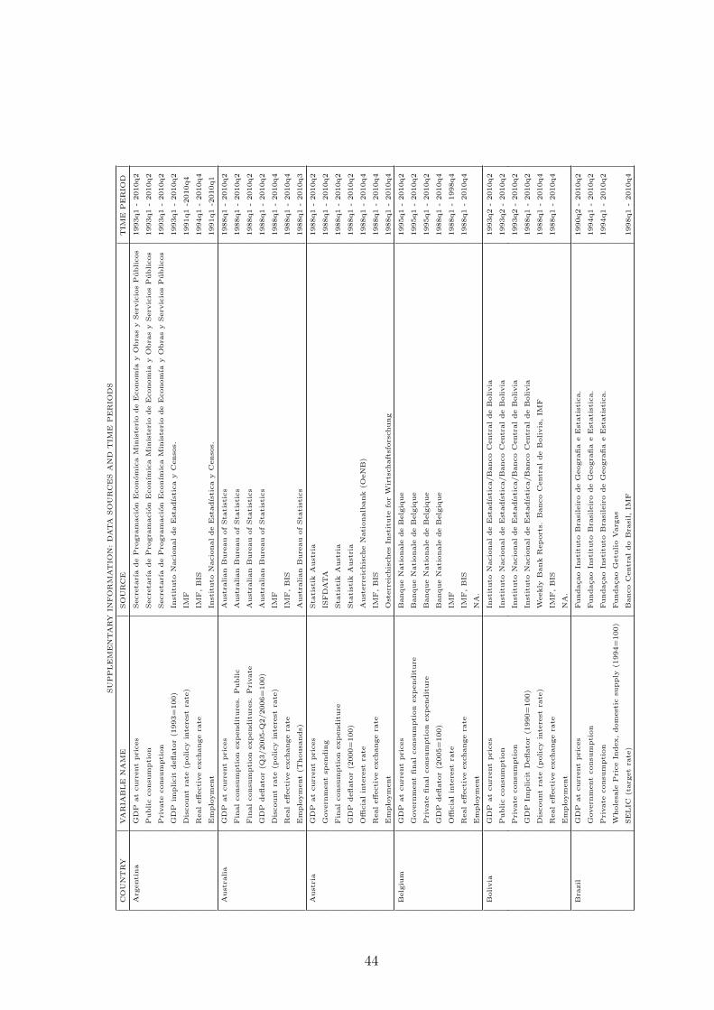
9The complete list of countries and periods for each series is listed in a separate supplement accom-panying this document.

10Countries where civilian employment is not available include (parentheses indicate the proxy usedin different controls): Brazil (economically active population), Ecuador (employment: global occupa-tion rate), Pakistan (total employment), Peru (employed in metropolitan Lima), and the Philippines(employment).

11A country is considered to have a fixed exchange rate if during 8 quarters or more it has no legaltender, hard pegs, crawling pegs, and de facto or pre-announced bands or crawling bands with marginsof no larger than +/- 2 percent. All other episodes are considered flexible.

8

rate regimes for the countries is shown in Table 3. We also follow IMV to classify a

country’s openness by a de-facto measure of a country’s trade ratio (defined as exports

plus imports to GDP). If a country’s ratio is greater than 60 percent it is considered open

(see Table 4 for a complete list of open and closed economies). We use the Reinhart and

Rogoff (2010) database of national debt to classify countries according to their ratios of

general government debt to GDP (see Table 5). We use a threshold of 60 percent above

which a country is classified as high-debt country. And, finally, we use the 2010 World

Bank classification of developing vs. high income countries.

Although the data set used by IMV is similar to the one used in this paper, there are

important differences between them. First, they use 44 countries and we use 55.12 The

second difference is that, while we have the same time period for all the sample, countries

in the IMV dataset have different time periods. Those features make our dataset 50%

larger than the IMV dataset: our total number of observations in the pooled data is about

3900 while the IMV dataset has around 2500.13 With respect to the quality of our data,

we rely on the reported values from central banks and statistical agencies. Although it

is true that some countries do not have over all the period the same methodology to

collect and report data as is the case in the IMV dataset, we obtain similar results to

IMV when we use the same sample of countries, suggesting data quality is comparable.

5 Results

Figure 1 shows statistically and significant positive multiplier estimates through all the

horizon of analysis.14 The impact multiplier is 0.36 and the long run multiplier is 0.92.

12The countries that appear in the IMV dataset but do not appear in our dataset are Botswana,Bulgaria, Croatia, Estonia, Israel, Latvia, Lithuania, Romania, Slovenia and Uruguay. It can be seenthat they are predominantly former Soviet Union countries (7 out of 10). At the same time, thecountries that appear in our data set but do not appear in the IMV dataset are Austria, Bolivia,China, Costa Rica, Guatemala, Hong Kong, India, Indonesia, Japan, Korea, Luxembourg, New Zealand,Pakistan, Paraguay, Philippines, the Russian Federation, Singapore, Switzerland, Taiwan, Venezuelaand Vietnam.

13The number of observations that we use in the main estimation is 3131. If we consider the IMVdata, only 2241 can be used with our estimator.

14We calculate two types of multipliers: the impact multiplier, which measures the change in out-put in response to a one unit change in government spending in a given quarter, and the cumulative

9

Those results hold whether we include or not the interest rate and the real exchange

rate, although the numbers show a small change. In principle, controlling for the interest

rate should isolate the effect of monetary and fiscal policy, but the small change in the

estimates for the multipliers suggest that on average the monetary authority does not

accommodate much to fiscal policy. To illustrate this point, Figure 2 shows the response

of output, interest rate and real exchange rate to a one unit standard deviation shock in

government spending.15 Although the interest rate decreases in the first quarter, it in-

creases afterwards and is not statistically different to zero, suggesting no accommodation

from the monetary authority after the first quarter of the shock. At the same time, the

real exchange rate depreciates in the first quarters, but its change is not different from

zero from the third quarter on of the shock. This suggests a non persistent effect in the

real exchange rate of higher demand and imports. Ravn et. al. (2012) also observe a de-

preciation of the exchange rate in response to an increase in government purchases, and

propose an explanation based on deep habits, who cause markups to decline in markets

with strong aggregate demand, such that when government spending increases, markups

fall on domestically sold goods, depreciating the exchange rate. Although those numbers

are not too big, they imply a positive response of output to government spending, and

may imply larger multipliers during some periods of the business cycles.

Positive multipliers are consistent in principle with both the Keynessian and neoclas-

sical models.16 In the neoclassical model (see for example Baxter and King (1993)), an

increase in government spending creates a negative wealth effect for households because

it has to be matched by an increase of taxes in the future. Individuals reduce con-

sumption and leisure because of the negative wealth effect, increasing at the same time

labor supply and driving down the wage rate. Higher labor supply, in turn, increases

multiplier, which measures the cumulative change in output divided by the cumulative change in gov-ernment spending over a determined time horizon. Because all our specifications are in logs, we haveto multiply those values by the ratio of average output to average government spending to obtain thefiscal multipliers.

15The impulse response function of the variable X with respect to the variable Y is the response ofthe variable X to a one unit standard deviation shock in the variable Y. The units are in percentagepoints. The confidence intervals represent 90% of the distribution (5% the lower and 95% the higher).

16Positive multipliers also suggest negative output effects of fiscal consolidations. Under specificcircumstances, those effects may occur (Giavazzi and Pagano (1990), Alesina and Ardagana (1998)),but on average for our sample, results suggest that is not the case.

10

output. The main difference between the neoclassical model and the new Keynesian

model comes from the response of private consumption, which decreases in the neoclas-

sical model but increases in the new Keynessian model. Consumption may increase in

the new Keynesian model when government spending increases because nonseparability

between consumption and leisure, because the aggregate demand for labor shifts with

counter-cyclical markups, because nominal rigidities, because increasing returns in pro-

duction or because rule of thumb consumers. The key issue is that consumption increases

when the real wage does not change or when it increases. This effect can be attained

when the labor demand curve shifts outwards, at the same time that the labor supply

shifts outwards, such that the real wage does not fall. The fact that the multipliers are

on average lower than 1 may suggest some crowding out because output rises less than

government spending. Another point to notice is that different sources of government

financing might have a different effect in the short and in the long run. Higher debt, for

example, could affect long-run sustainability and thus current fiscal policy as well.

We find that private consumption responds positively to government spending in our

panel of countries, giving support to the Keynesian theories (see figures 3 and 4).17

Although always positive, this response in statistically significant only until the third

year, suggesting that probably the effects on consumption dilute with time. Consistent

with theory, we find that employment increases in all cases. This result is consistent

with the result that Blanchard and Perotti (2002) find for the United States, but is

the opposite of the results of Ramey and Shapiro (1997), Edelberg et al (1999) and

Ramey (2009). Ramey argues that the differences come from anticipation effects: once

she controls for expectations using the identification strategy of Blanchard and Perotti

(2002), private consumption actually falls. Our results are not particular to one country

or to a small number of episodes: we use a large sample of countries and correct for

additional potential biases coming from third factors affecting output and government

spending.

17Non-keynesian effects of fiscal policy, however, are not ruled out because of this result. Those effectsmay come, for example, through changes in expectations, credibility and interest rate premiums andlack of wealth effects on labor supply (Barry and Devereux, 2003). In fact, for our sample as shownlater, high-debt countries have a lower fiscal multipliers; this may come from of credibility concerns.

11

We next analyze the fiscal multipliers for countries operating in flexible vs. fixed

exchange rate regimes. When we do not control for the interest rate or the real exchange

rate, the impact and cumulative multipliers are statistically different throughout all

the time of analysis (figure 5). The impact multipliers are 0.57 and 0.27 in the case

of the fixed and flexible exchange rates, respectively, and the difference is statistically

significant. In a 5 year horizon, the cumulative multipliers are 1.58 and -0.27 respectively.

However, in the case of countries operating under flexible exchange rates, the multiplier

is not statistically different from zero except during the first year, a period in which it is

positive. IMV obtain the same relative results, although they get a negative cumulative

multiplier in the case of the flexible exchange rate regimes, and we do not. It is interesting

to note that once we control for the interest rate and the real exchange rate (figure 6), the

statistical differences disappear between multipliers. This shows that their differences

do come from the behavior of the real exchange rate and the interest rate. At the same

time, the fiscal multipliers for the countries operating under fixed exchange rates are

always statistically different from zero and positive, while they are not different from

zero for countries operating under flexible exchange rates.

Those results are in principle consistent with the Mundell Fleming model. Under

flexible exchange rate regimes, an increase in government spending causes an apprecia-

tion of the real exchange rate given an increase in imports relative to exports. Under

fixed exchange rates, the monetary authority intervenes to prevent this appreciation

by expanding the money supply. Figure 7 shows the response of such variables to a

shock in government spending. In the case of the flexible exchange rate countries, we

observe an appreciation of the real exchange rate as the theory predicts. In the case of

the countries operating under fixed exchange rate regimes we do not observe monetary

accommodation. We observe an initial real exchange rate depreciation that disappears

after the first quarter that may be explained by the mechanism proposed by Ravn et al.

(2012) as explained before.

We next analyze the response of economies that differ in their degree of trade open-

ness. Figure 8 shows impact multipliers that are statistically positive and different

12

between both cases (0.62 for closed economies and 0.37 for open economies). Long

run multipliers have positive point estimates, but they are statistically positive only for

closed economies. Although they are statistically not distinguishable from each other

after the first year, the uncertainty is higher in the case of the open economies. Those

results are consistent with IMV, although our point estimates are higher and nonnega-

tive in both cases while they find negative multipliers in the case of the open economies.

Those results are also consistent in principle with the Mundell Fleming model. In the

case of open economies, this model predicts that part of the demand generated by an

increase in government spending should go to imported goods, ameliorating the domestic

output response. This also implies an appreciation of the real exchange rate, which is

what we observe in figure 9 after the third quarter.

Figure 10 shows the differences between the fiscal multipliers of high-income vs. de-

veloping countries. We find that the impact multipliers are both positive and not sta-

tistically different. In the long run, the fiscal multiplier for developing countries is 0.88,

suggesting some degree of crowding out because output rises less than total government

spending. This multiplier is statistically different from zero. In the case of high-income

countries, we find that the fiscal multiplier is positive although not statistically different

from zero. Those results are in contrast to IMV, who find a negative multiplier not

statistically different from zero for developing countries and positive multipliers for high

income countries. Interestingly, figure 11 shows that the fiscal multipliers are both sta-

tistically different form zero during the first 3 years if we do not control for either the

interest rate or the real exchange rate, suggesting the importance of those variables. The

same figure shows that if we do not control for the interest rate or the real exchange rate,

impact multipliers are both positive and statistically different. To precisely analyze the

mechanisms behind this behavior, figure 12 shows how in the case of developing coun-

tries the interest rate increases after an initial negative response, suggesting an initial

accommodation from the monetary authority. In the case of the high-income countries,

there is also an initial accommodation of the monetary authority, but it is zero after

the third quarter throughout all the period of analysis. In the case of the real exchange

rate, the only change that is distinguishable from zero is in the case of the developing

13

countries, where we can observe a depreciation of this index in the first quarters. The

picture that emerges is that the crowding out effect, although present in both cases, is

bigger in the case of high income countries, a result in contrast with previous studies.

We think those results are more in line with the notion that developing countries have

more binding constraints to spending that can be alleviated with fiscal stimulus.

The level of indebtedness may influence the effect of government spending on output.

The intuition is that a high level of debt may affect the expectations about repayment

and about future fiscal adjustment, counteracting the expansionary effects of an increase

in government spending. Figure 13 shows that the fiscal stimulus is more effective in

countries with a low level of debt: the multiplier in the long run is 1.49 in the case of

low debt countries vs. 0.39 in the case of high debt countries, and the impact multiplier

is 0.44 vs 0.37, respectively. After the third quarter, however, the multiplier for high

debt countries is not different from zero, while it is zero in in the case of low debt

countries. Although changes in the interest rate and the real exchange rate are not

statistically different from zero (figure 14), the point estimates suggest that an increase

in government spending in a high debt country may either signal difficulty of payment

later or inflationary concerns, as the increase in the interest rate suggests.

5.1 Sources of divergence with previous results

We investigate in this section the factors that explain the divergence with previous

results, specifically the differences with the results of IMV. In order to make the com-

parisons possible through all the empirical exercises of this section, we do not use per

capita data as we have done so far in the paper and instead we use aggregate data, we

calculate the multiplier discounting it by the median interest rate as IMV, and we use the

same variables that they use in the estimation, changing the discount rate that we used

in previous estimations with the current account measure. We take the IMV dataset

from the public version posted with their publication. Using the IMV dataset, we are

able to replicate the results for each of the cases reported in their paper. We calculate

the aggregate multipliers in their case to facilitate comparissons with our results.

14

We start by calculating the average multipliers for all the IMV sample of countries

using an OLS estimator (this is the original estimation in their paper) and the panel

SVAR estimator that we use in this paper. Figure 15 shows that the biases in the point

estimates are considerable in the long run: while the OLS estimator produces an average

multiplier 0.26, the panel SVAR estimator produces a multiplier of -0.4. The bias reflects

that the error term capturing shocks to output is positively correlated with government

spending, as expected. The confidence intervals overlap, and the GMM estimator has

much bigger standard errors due to the bootstrapping procedure we use. The fact that

the panel SVAR estimator produces even lower multipliers than the OLS estimator does

not explain the differences in the results, given that although we use this estimator, we

generally obtain much higher multipliers than Ilzetzki et al. If anything, the use of this

estimator reduces the differences between our results and their results.

We next analyze the effect of having different countries in the samples. As we will

show, this is the key factor explaining the differences in results. We create a panel with

the IMV data that only considers countries present in our data. In total, 34 countries are

present in both datasets. The countries present in the IMV dataset but not in ours are are

Botswana, Bulgaria, Croatia, Estonia, Israel, Latvia, Lithuania, Romania, Slovenia and

Uruguay. The countries present in our data set but not in the IMV dataset are Austria,

Bolivia, China, Costa Rica, Guatemala, Hong Kong, India, Indonesia, Japan, Korea,

Luxembourg, New Zealand, Pakistan, Paraguay, Philippines, the Russian Federation,

Singapore, Switzerland, Taiwan, Venezuela and Vietnam. Figure 16 shows the results

of estimating the fiscal multipliers with this common set of countries and compares it

with the multipliers estimated with all the countries present in each dataset. The upper

panel compares the fiscal multipliers when we use the original set of countries and the

panel SVAR estimator. As we have shown before, the IMV sample produces a multiplier

of 0.05 in the short run and -0.40 in the long run (not statistically different from zero),

while we obtain a multiplier of 0.43 in the short run and of 0.83 in the long run (both

statistically different from zero).18 The lower panel shows the same estimation with the

18Those numbers differ slightly from the previously reported multipliers because we use the currentaccount instead of the discount rate and because we use aggregate data instead of per capital data.

15

common set of countries. Results are very similar: Using the IMV data, we obtain a

fiscal multiplier of 0.40 and 0.43 in the short and in the long run, statistically different

from zero through almost in the entire period. We obtain with our data fiscal multipliers

of 0.52 and 0.54 in the short and the long run. The confidence intervals vastly overlap.

It is clear from this figure that the sample composition explains almost all the differences

between our results and the results of IMV.

When we use the same sample of countries present in both datasets to analyze the

multipliers in developing vs high income countries, we still obtain positive fiscal mul-

tipliers in the short run, a result that is different to their results, although it is lower

than the multipliers of high income countries and zero in the long run as it is shown in

Figure 17. In the other cases (debt, exchange rate regime and degree of trade openness),

we obtained similar results than the ones at the beginning of section 5. 19. Table 6

summarizes the results presented in figures 15 and 16, namely that sample selection is

the main driver of the differences between our estimates and IMV results.

6 Conclusions

We use quarterly data in a panel of 55 countries between 1988 and 2010 to analyze the

effect of shocks to government spending on GDP and private consumption. In addition

to using a more comprehensive dataset than previous studies, as an additional innovation

we use panel SVAR techniques to correct for the correlation of the explanatory variables

with the error terms known to be present in this type of settings. This helps to ameliorate

other possible sources of endogeneity like anticipation effects of third variables that may

affect both output and government spending.

We find positive multipliers of around 0.3 on impact and between 0.9 and 1.0 in the

long run. In addition, we find positive private consumption and employment responses,

giving support to Keynessian theories. Those numbers, although not larger than one,

19We also changed the time period and dropped the crisis years between 2008 and 2010. The periodof analysis did not have almost any effect on the results.

16

show that fiscal policy can be effective stimulating the economy, an important policy

issue especially in times of economic turmoil. A short run-multiplier bigger than zero

gives support to a countercyclical fiscal policy. A long-run multiplier bigger than zero

is important to ensure that countercyclical fiscal policy does not have negative long-

run effects. At the end, with the possibility that fiscal multipliers are lower than one

(although positive) policymakers should weight the benefits of fiscal policy under times

of economic stress versus the potential displacement of private investment that could

have other long-run effects.

Results in this paper question previous conclusions drawn in the panel VAR literature

that analyzes fiscal multipliers. The type of estimator and the sample selection are

important drivers of those conclusions. Contrary to previous research,we find that the

fiscal multiplier is larger in developing than in high-income countries, that it is zero in

high debt countries and in countries operating under flexible exchange rates (instead

of negative), and we do not find strong evidence of monetary accommodation. The

differences between our results and those of previous studies come fundamentally from

the sample of countries. The use of a GMM estimator instead of an OLS estimator also

shows that OLS estimators induce some important biases in the results.

17

References

[1] Alesina, Alberto and Ardagna, Silvia, 1998. “Tales of Fiscal Adjustment,” Economic

Policy, vol. 0(27), pages 73 - 86.

[2] Auerbach, Alan and Yuriy Gorodnichenko, 2012. “Measuring the Output Responses

to Fiscal Policy,” American Economic Journal: Economic Policy, American Economic

Association, vol. 4(2), pages 1 - 27.

[3] Barro, Robert and Charles Redlick, 2011. “Macroeconomic Effects from Government

Purchases and Taxes,” Quarterly Journal of Economics, vol. 127(3), pages 829 - 887.

[4] Barry, Frank and Devereux, Michael, 2013. “Expansionary Fiscal Contraction: A

Theorethical Exploration,” Journal of Macroeconomics, vol. 25(1), pages 1 - 23.

[5] Beetsma, Roel and Massimo Giuliodori, 2011. “The Effects of Government Purchases

Shocks: Review and Estimates for the EU,” Economic Journal, Royal Economic So-

ciety, vol. 121(550), pages F4 - F32.

[6] Blanchard, Olivier and Roberto Perotti, 2002. “An Empirical Characterization of

the Dynamic Effects of Changes in Government Spending and Taxes on Output,”

Quarterly Journal of Economics (November), pages 1329 - 1368.

[7] Edelberg, Wendy, Martin Eichenbaum and Jonas D. M. Fisher, 1999. “Understanding

the Effects of a Shock to Government Purchases,” Review of Economic Dynamics 2

(January), pages 166 - 206.

[8] Fatıs, Antonio and Mihov, Ilian, 2001. “The Effects of Fiscal Policy on Consumption

and Employment: Theory and Evidence,” CEPR Discussion Papers 2760.

[9] Giavazzi, Francesco and Pagano, Marco, 1990. “Can Severe Fiscal Contractions be

Expansionary? Tales from two Small European Economies,” NBER Macroeconomics

Annual.

18

[10] Holtz-Eakin, Douglas and Newey, Whitney and Rosen, Harvey S, 1988. “Estimating

Vector Autoregressions with Panel Data,” Econometrica, Econometric Society, vol.

56(6), pages 1371 - 95.

[11] Ilzetzki, Ethan, Carlos Vegh and Enrique Mendoza, 2013 “How Big (Small?) are

Fiscal Multipliers?,” Journal of Monetary Economics, vol. 60(2), pages 239 - 254.

[12] Ilzetzki, Ethan, Carmen Reinhart and Kenneth Rogoff, 2008. “De-facto exchange

rate classification 1945-2010” in “Exchange Rate Arrangements Entering the 21st

Century: Which Anchor Will Hold?”

[13] Judson, Ruth A. and Ann L. Owen, 1999 “Estimating Dynamic Panel Data Models:

A Guide for Macroeconomists,” Economic Letters, vol. 65, pages 9 - 15.

[14] Love, Inessa and Zicchino, Lea, 2006. “Financial development and dynamic invest-

ment behavior: Evidence from panel VAR,” The Quarterly Review of Economics and

Finance, Elsevier, vol. 46(2), pages 190 - 210.

[15] Merten, Karel and Morten Ravn, 2012. “Empirical evidence on the aggregate effects

of anticipated and unanticipated U.S. tax policy shocks,” American Economic Journal:

Economic POlicy, vol 4(2), pages 27 - 64

[16] Mountford, Andrew and Harald Uhlig, 2009. “What are the effects of fiscal policy

shocks?,” Journal of Applied Econometrics, vol. 24(6), pages 960 - 992.

[17] Nakamura, Emi and Jon Steinsson, 2011. “Fiscal Stimulus in a Monetary Union,”

NBER Working paper 17391.

[18] Perotti, Roberto, 2005. “Estimating the Effects of Fiscal Policy in OECD Coun-

tries,” CEPR Discussion Paper 4842.

[19] Ramey, Valerie A. and Matthew Shapiro, 1998. “Costly Capital Reallocation and

the Effects of Government Spending,” Carnegie Rochester Conference on Public Pol-

icy.

19

[20] Ramey, Valerie A., 2011. “Identifying government spending shocks: it’s all in the

timing,” Quarterly Journal of Economics, vol. 126(1), pages 1 - 50.

[21] Ravn, Morten, Stephanie Schmitt-Grohe and Martın Uribe, 2012. “Explaining the

Effects of Government Spending Shocks,” Journal of Monetary Economics, vol. 59(3),

pages 215 - 34.

[22] Reinhart, Carmen and Kenneth Rogoff, 2010. Tables in “From Financial Crisis to

Debt Crises,” NBER WP 15795.

[23] Suarez-Serrato, Juan Carlos and Philippe Wingender, 2011. “Estimating Local Fis-

cal Multipliers,” Working paper, University of California, Berkeley.

20

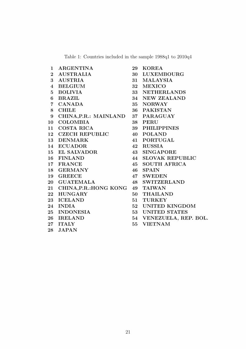
Table 1: Countries included in the sample 1988q1 to 2010q4

1 ARGENTINA 29 KOREA2 AUSTRALIA 30 LUXEMBOURG3 AUSTRIA 31 MALAYSIA4 BELGIUM 32 MEXICO5 BOLIVIA 33 NETHERLANDS6 BRAZIL 34 NEW ZEALAND7 CANADA 35 NORWAY8 CHILE 36 PAKISTAN9 CHINA,P.R.: MAINLAND 37 PARAGUAY

10 COLOMBIA 38 PERU11 COSTA RICA 39 PHILIPPINES12 CZECH REPUBLIC 40 POLAND13 DENMARK 41 PORTUGAL14 ECUADOR 42 RUSSIA15 EL SALVADOR 43 SINGAPORE16 FINLAND 44 SLOVAK REPUBLIC17 FRANCE 45 SOUTH AFRICA18 GERMANY 46 SPAIN19 GREECE 47 SWEDEN20 GUATEMALA 48 SWITZERLAND21 CHINA,P.R.:HONG KONG 49 TAIWAN22 HUNGARY 50 THAILAND23 ICELAND 51 TURKEY24 INDIA 52 UNITED KINGDOM25 INDONESIA 53 UNITED STATES26 IRELAND 54 VENEZUELA, REP. BOL.27 ITALY 55 VIETNAM28 JAPAN

21

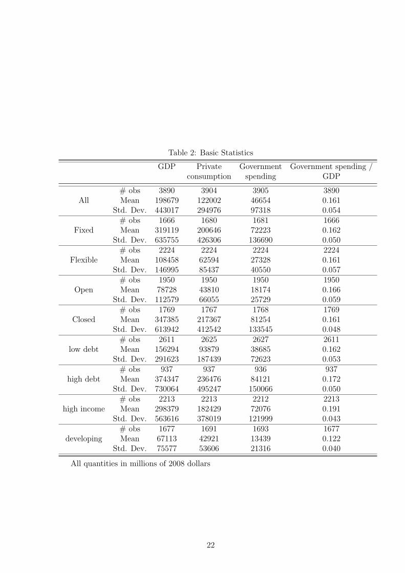
Table 2: Basic Statistics

GDP Private Government Government spending /consumption spending GDP

# obs 3890 3904 3905 3890All Mean 198679 122002 46654 0.161

Std. Dev. 443017 294976 97318 0.054# obs 1666 1680 1681 1666

Fixed Mean 319119 200646 72223 0.162Std. Dev. 635755 426306 136690 0.050

# obs 2224 2224 2224 2224Flexible Mean 108458 62594 27328 0.161

Std. Dev. 146995 85437 40550 0.057# obs 1950 1950 1950 1950

Open Mean 78728 43810 18174 0.166Std. Dev. 112579 66055 25729 0.059

# obs 1769 1767 1768 1769Closed Mean 347385 217367 81254 0.161

Std. Dev. 613942 412542 133545 0.048# obs 2611 2625 2627 2611

low debt Mean 156294 93879 38685 0.162Std. Dev. 291623 187439 72623 0.053

# obs 937 937 936 937high debt Mean 374347 236476 84121 0.172

Std. Dev. 730064 495247 150066 0.050# obs 2213 2213 2212 2213

high income Mean 298379 182429 72076 0.191Std. Dev. 563616 378019 121999 0.043

# obs 1677 1691 1693 1677developing Mean 67113 42921 13439 0.122

Std. Dev. 75577 53606 21316 0.040

All quantities in millions of 2008 dollars

22

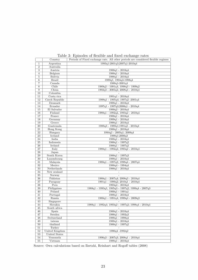
Table 3: Episodes of flexible and fixed exchange ratesCountry Periods of Fixed exchange rate. All other periods are considered flexible regimes

1 Argentina 1993q1:2001q3;2007q1-2010q42 Australia -3 Austria 1988q1 - 2010q44 Belgium 1988q1 - 2010q45 Bolivia 1988q1 - 2010q46 Brazil 1989q1; 1994q3-1998q47 Canada 1988q1-2001q48 Chile 1989q2 - 1991q4; 1998q3 - 1999q29 China 1992q3 - 2005q2; 2008q4 - 2010q410 Colombia -11 Costa rica 1991q1 - 2010q412 Czech Republic 1988q1 - 1995q4; 1997q2 -2001q413 Denmark 1988q1 - 2010q414 Ecuador 1997q1 - 1997q3;2000q1 - 2010q415 El Salvador 1990q2 - 2010q416 Finland 1988q1 - 1992q2, 1993q2 - 2010q417 France 1988q1 - 2010q418 Germany 1999q1 - 2010q419 Greece 1988q1 - 2010q420 Guatemala 1988q3 - 1989q1;1991q2 - 2010q421 Hong Kong 1988q1 - 2010q422 Hungary 1994q2 - 2005q1; 2009q423 Iceland 1988q1:2000q324 India 1988q1 - 2010q425 Indonesia 1988q1 - 1997q226 Ireland 1988q1 - 1997q227 Italy 1988q1 - 1992q2; 1993q2 - 2010q428 Japan -29 South Korea 1988q1 - 1997q330 Luxembourg 1988q1 - 2010q431 Malaysia 1988q1 - 1997q2; 1998q4 - 2007q432 Mexico 1988q4 - 1994q433 Netherlands 1988q1 - 2010q434 New zealand -35 Norway -36 Pakistan 1988q1 - 2007q4; 2008q3 - 2010q437 Paraguay 1991q1 - 1999q2; 2010q1 - 2010q438 Peru 1993q4 - 2010q439 Philippines 1988q1 - 1993q1; 1995q3 - 1997q2; 1999q4 - 2007q340 Poland 1990q1 - 1991q141 Portugal 1988q1 - 2010q442 Russia 1988q1 - 1991q4; 1999q4 - 2009q343 Singapore -44 Slovakia 1988q1 - 1992q4; 1993q2 - 1997q2; 1998q4 - 2010q445 South africa -46 Spain 1988q1 - 2010q447 Sweden 1988q1 - 1992q348 Switzerland 1988q1 - 1998q449 taiwan 1988q1 - 2010q450 thailand 1988q1 - 1997q251 Turkey -52 United Kingdom 1990q4 -1992q253 United States -54 Venezuela 1996q3 - 2007q3; 2008q1 - 2010q455 Vietnam 1988q1 - 2010q4

Source: Own calculations based on Ilzetzki, Reinhart and Rogoff tables (2008)

23

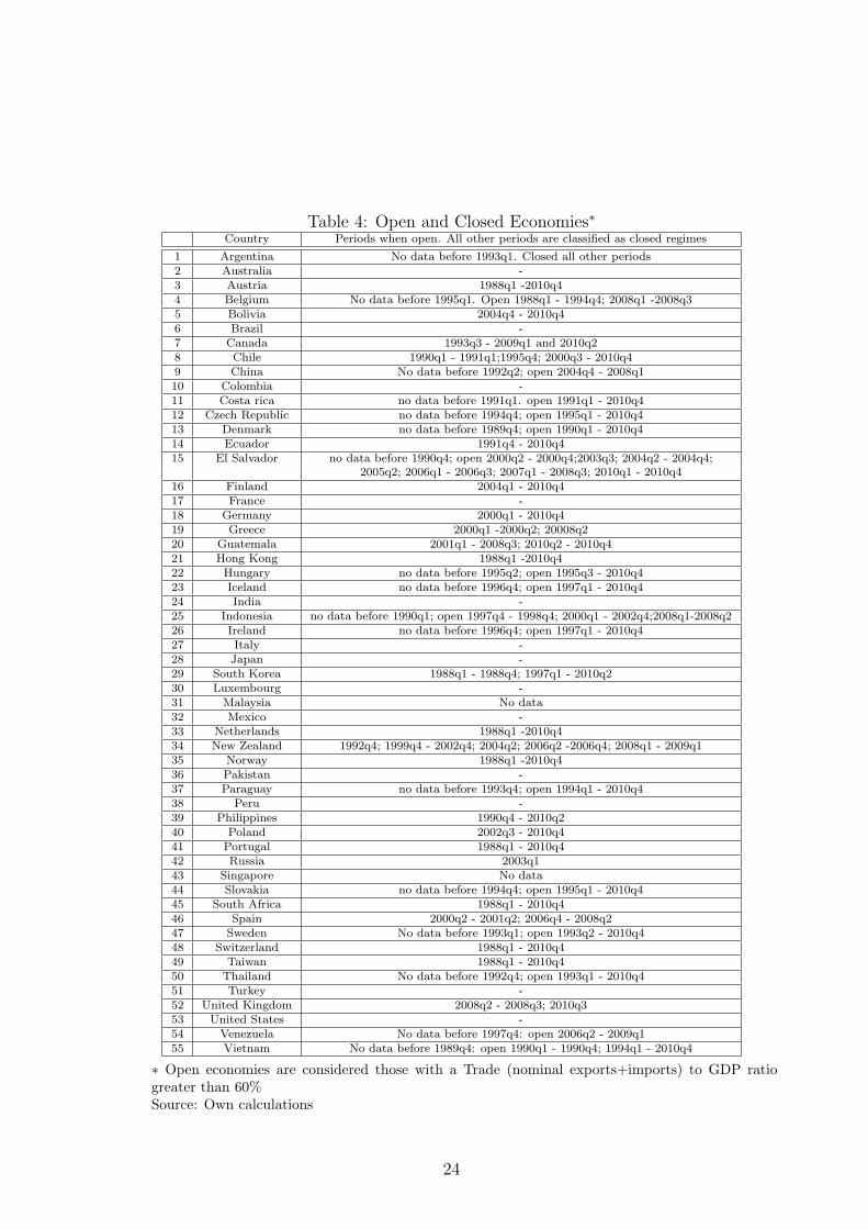
Table 4: Open and Closed Economies∗Country Periods when open. All other periods are classified as closed regimes

1 Argentina No data before 1993q1. Closed all other periods2 Australia -3 Austria 1988q1 -2010q44 Belgium No data before 1995q1. Open 1988q1 - 1994q4; 2008q1 -2008q35 Bolivia 2004q4 - 2010q46 Brazil -7 Canada 1993q3 - 2009q1 and 2010q28 Chile 1990q1 - 1991q1;1995q4; 2000q3 - 2010q49 China No data before 1992q2; open 2004q4 - 2008q110 Colombia -11 Costa rica no data before 1991q1. open 1991q1 - 2010q412 Czech Republic no data before 1994q4; open 1995q1 - 2010q413 Denmark no data before 1989q4; open 1990q1 - 2010q414 Ecuador 1991q4 - 2010q415 El Salvador no data before 1990q4; open 2000q2 - 2000q4;2003q3; 2004q2 - 2004q4;

2005q2; 2006q1 - 2006q3; 2007q1 - 2008q3; 2010q1 - 2010q416 Finland 2004q1 - 2010q417 France -18 Germany 2000q1 - 2010q419 Greece 2000q1 -2000q2; 20008q220 Guatemala 2001q1 - 2008q3; 2010q2 - 2010q421 Hong Kong 1988q1 -2010q422 Hungary no data before 1995q2; open 1995q3 - 2010q423 Iceland no data before 1996q4; open 1997q1 - 2010q424 India -25 Indonesia no data before 1990q1; open 1997q4 - 1998q4; 2000q1 - 2002q4;2008q1-2008q226 Ireland no data before 1996q4; open 1997q1 - 2010q427 Italy -28 Japan -29 South Korea 1988q1 - 1988q4; 1997q1 - 2010q230 Luxembourg -31 Malaysia No data32 Mexico -33 Netherlands 1988q1 -2010q434 New Zealand 1992q4; 1999q4 - 2002q4; 2004q2; 2006q2 -2006q4; 2008q1 - 2009q135 Norway 1988q1 -2010q436 Pakistan -37 Paraguay no data before 1993q4; open 1994q1 - 2010q438 Peru -39 Philippines 1990q4 - 2010q240 Poland 2002q3 - 2010q441 Portugal 1988q1 - 2010q442 Russia 2003q143 Singapore No data44 Slovakia no data before 1994q4; open 1995q1 - 2010q445 South Africa 1988q1 - 2010q446 Spain 2000q2 - 2001q2; 2006q4 - 2008q247 Sweden No data before 1993q1; open 1993q2 - 2010q448 Switzerland 1988q1 - 2010q449 Taiwan 1988q1 - 2010q450 Thailand No data before 1992q4; open 1993q1 - 2010q451 Turkey -52 United Kingdom 2008q2 - 2008q3; 2010q353 United States -54 Venezuela No data before 1997q4: open 2006q2 - 2009q155 Vietnam No data before 1989q4: open 1990q1 - 1990q4; 1994q1 - 2010q4

∗ Open economies are considered those with a Trade (nominal exports+imports) to GDP ratiogreater than 60%Source: Own calculations

24

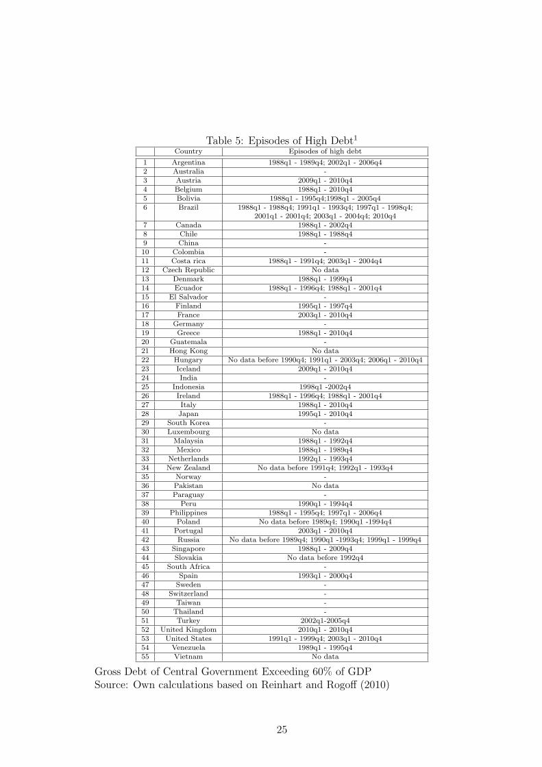
Table 5: Episodes of High Debt1

Country Episodes of high debt

1 Argentina 1988q1 - 1989q4; 2002q1 - 2006q42 Australia -3 Austria 2009q1 - 2010q44 Belgium 1988q1 - 2010q45 Bolivia 1988q1 - 1995q4;1998q1 - 2005q46 Brazil 1988q1 - 1988q4; 1991q1 - 1993q4; 1997q1 - 1998q4;

2001q1 - 2001q4; 2003q1 - 2004q4; 2010q47 Canada 1988q1 - 2002q48 Chile 1988q1 - 1988q49 China -10 Colombia -11 Costa rica 1988q1 - 1991q4; 2003q1 - 2004q412 Czech Republic No data13 Denmark 1988q1 - 1999q414 Ecuador 1988q1 - 1996q4; 1988q1 - 2001q415 El Salvador -16 Finland 1995q1 - 1997q417 France 2003q1 - 2010q418 Germany -19 Greece 1988q1 - 2010q420 Guatemala -21 Hong Kong No data22 Hungary No data before 1990q4; 1991q1 - 2003q4; 2006q1 - 2010q423 Iceland 2009q1 - 2010q424 India -25 Indonesia 1998q1 -2002q426 Ireland 1988q1 - 1996q4; 1988q1 - 2001q427 Italy 1988q1 - 2010q428 Japan 1995q1 - 2010q429 South Korea -30 Luxembourg No data31 Malaysia 1988q1 - 1992q432 Mexico 1988q1 - 1989q433 Netherlands 1992q1 - 1993q434 New Zealand No data before 1991q4; 1992q1 - 1993q435 Norway -36 Pakistan No data37 Paraguay -38 Peru 1990q1 - 1994q439 Philippines 1988q1 - 1995q4; 1997q1 - 2006q440 Poland No data before 1989q4; 1990q1 -1994q441 Portugal 2003q1 - 2010q442 Russia No data before 1989q4; 1990q1 -1993q4; 1999q1 - 1999q443 Singapore 1988q1 - 2009q444 Slovakia No data before 1992q445 South Africa -46 Spain 1993q1 - 2000q447 Sweden -48 Switzerland -49 Taiwan -50 Thailand -51 Turkey 2002q1-2005q452 United Kingdom 2010q1 - 2010q453 United States 1991q1 - 1999q4; 2003q1 - 2010q454 Venezuela 1989q1 - 1995q455 Vietnam No data

Gross Debt of Central Government Exceeding 60% of GDPSource: Own calculations based on Reinhart and Rogoff (2010)

25

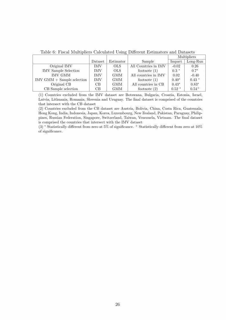
Table 6: Fiscal Multipliers Calculated Using Different Estimators and DatasetsMultipliers

Dataset Estimator Sample Impact Long-RunOriginal IMV IMV OLS All Countries in IMV -0.02 0.26

IMV Sample Selection IMV OLS footnote (1) 0.3 ∗ 0.7∗

IMV GMM IMV GMM All countries in IMV 0.02 -0.40IMV GMM + Sample selection IMV GMM footnote (1) 0.40∗ 0.43 ∗

Original CB CB GMM All countries in CB 0.43∗ 0.83∗

CB Sample selection CB GMM footnote (2) 0.52 ∗ 0.54+

(1) Countries excluded from the IMV dataset are Botswana, Bulgaria, Croatia, Estonia, Israel,Latvia, Lithuania, Romania, Slovenia and Uruguay. The final dataset is comprised of the countriesthat intersect with the CB dataset(2) Countries excluded from the CB dataset are Austria, Bolivia, China, Costa Rica, Guatemala,Hong Kong, India, Indonesia, Japan, Korea, Luxembourg, New Zealand, Pakistan, Paraguay, Philip-pines, Russian Federation, Singapore, Switzerland, Taiwan, Venezuela, Vietnam. The final datasetis comprised the countries that intersect with the IMV dataset(3) ∗ Statistically different from zero at 5% of significance. + Statistically different from zero at 10%of significance.

26

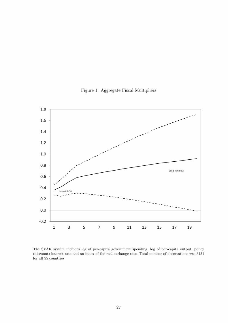
Figure 1: Aggregate Fiscal Multipliers

-0.2

0.0

0.2

0.4

0.6

0.8

1.0

1.2

1.4

1.6

1.8

1 3 5 7 9 11 13 15 17 19

Impact: 0.36

Long-run: 0.92

The SVAR system includes log of per-capita government spending, log of per-capita output, policy(discount) interest rate and an index of the real exchange rate. Total number of observations was 3131for all 55 countries

27

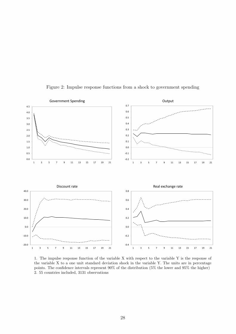
Figure 2: Impulse response functions from a shock to government spending

0.0

0.5

1.0

1.5

2.0

2.5

3.0

3.5

4.0

4.5

1 3 5 7 9 11 13 15 17 19 21

Government Spending

-0.2

-0.1

0.0

0.1

0.2

0.3

0.4

0.5

0.6

0.7

1 3 5 7 9 11 13 15 17 19 21

Output

-20.0

-10.0

0.0

10.0

20.0

30.0

40.0

1 3 5 7 9 11 13 15 17 19 21

Discount rate

-0.4

-0.2

0.0

0.2

0.4

0.6

0.8

1 3 5 7 9 11 13 15 17 19 21

Real exchange rate

1. The impulse response function of the variable X with respect to the variable Y is the response ofthe variable X to a one unit standard deviation shock in the variable Y. The units are in percentagepoints. The confidence intervals represent 90% of the distribution (5% the lower and 95% the higher)2. 55 countries included, 3131 observations

28

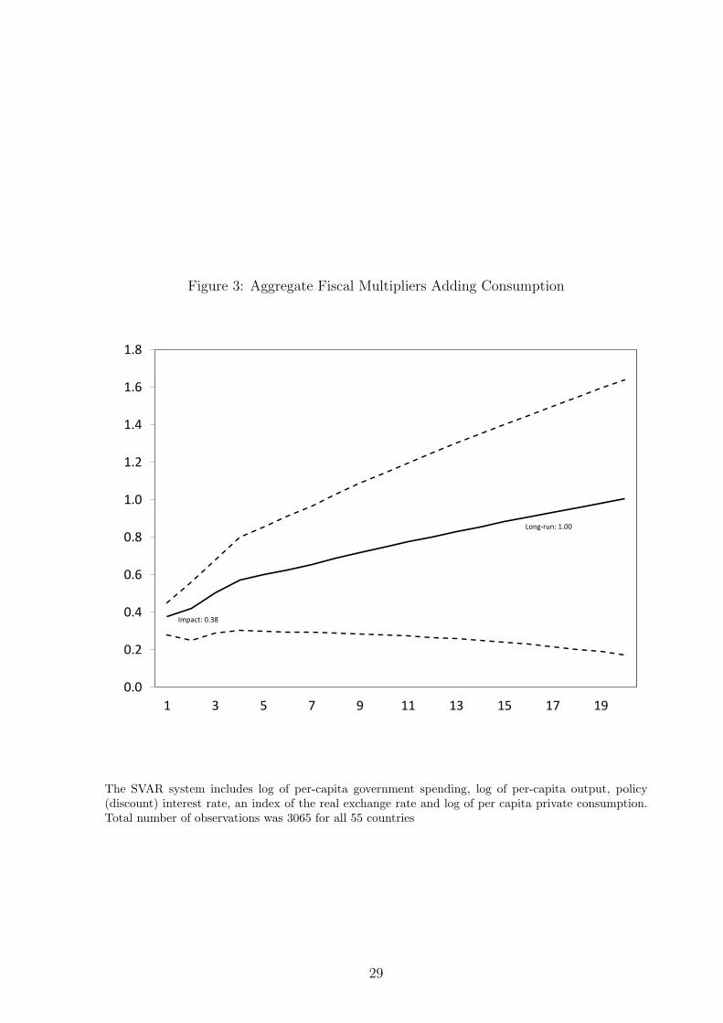
Figure 3: Aggregate Fiscal Multipliers Adding Consumption

0.0

0.2

0.4

0.6

0.8

1.0

1.2

1.4

1.6

1.8

1 3 5 7 9 11 13 15 17 19

Impact: 0.38

Long-run: 1.00

The SVAR system includes log of per-capita government spending, log of per-capita output, policy(discount) interest rate, an index of the real exchange rate and log of per capita private consumption.Total number of observations was 3065 for all 55 countries

29

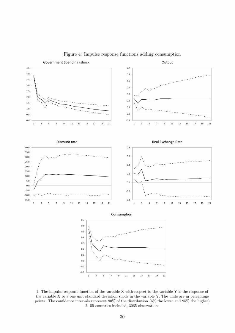
Figure 4: Impulse response functions adding consumption

0.0

0.5

1.0

1.5

2.0

2.5

3.0

3.5

4.0

4.5

1 3 5 7 9 11 13 15 17 19 21

Government Spending (shock)

-0.1

0.0

0.1

0.2

0.3

0.4

0.5

0.6

0.7

1 3 5 7 9 11 13 15 17 19 21

Output

-15.0

-10.0

-5.0

0.0

5.0

10.0

15.0

20.0

25.0

30.0

35.0

40.0

1 3 5 7 9 11 13 15 17 19 21

Discount rate

-0.4

-0.2

0.0

0.2

0.4

0.6

0.8

1 3 5 7 9 11 13 15 17 19 21

Real Exchange Rate

-0.2

-0.1

0.0

0.1

0.2

0.3

0.4

0.5

0.6

0.7

1 3 5 7 9 11 13 15 17 19 21

Consumption

1. The impulse response function of the variable X with respect to the variable Y is the response ofthe variable X to a one unit standard deviation shock in the variable Y. The units are in percentagepoints. The confidence intervals represent 90% of the distribution (5% the lower and 95% the higher)

2. 55 countries included, 3065 observations

30

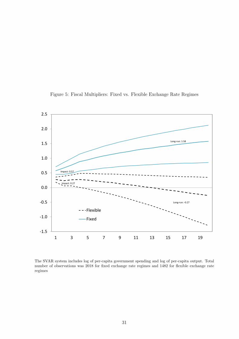
Figure 5: Fiscal Multipliers: Fixed vs. Flexible Exchange Rate Regimes

-1.5

-1.0

-0.5

0.0

0.5

1.0

1.5

2.0

2.5

1 3 5 7 9 11 13 15 17 19

Flexible

Fixed

Impact: 0.57

Impact: 0.27

Long-run: 1.58

Long-run: -0.27

The SVAR system includes log of per-capita government spending and log of per-capita output. Totalnumber of observations was 2018 for fixed exchange rate regimes and 1482 for flexible exchange rateregimes

31

Figure 6: Fiscal Multipliers: Flexible vs. Fixed exchange rate regimes Controlling forReal Interest Rate and Real Exchange Rate

-2.5

-2.0

-1.5

-1.0

-0.5

0.0

0.5

1.0

1.5

2.0

2.5

1 3 5 7 9 11 13 15 17 19

Flexible

Fixed

Impact: 0.41

Impact: 0.29

Long-run: 0.54

Long-run: 1.06

Discount rate and real exchange rate included

The SVAR system includes log of per-capita government spending, log of per-capita output, policy(discount) interest rate and an index of the real exchange rate. Total number of observations was 1516for fixed exchange rate regimes and 1469 for flexible exchange rate regimes

32

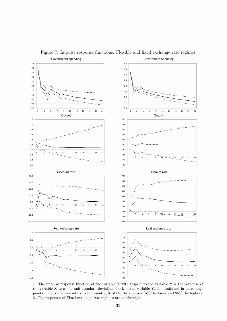
Figure 7: Impulse response functions: Flexible and fixed exchange rate regimes

-0.5

0.0

0.5

1.0

1.5

2.0

2.5

3.0

3.5

4.0

4.5

1 3 5 7 9 11 13 15 17 19 21

Government spending

0.0

0.5

1.0

1.5

2.0

2.5

3.0

3.5

4.0

1 3 5 7 9 11 13 15 17 19 21

Government Spending

-0.6

-0.4

-0.2

0.0

0.2

0.4

0.6

0.8

1.0

1.2

1 3 5 7 9 11 13 15 17 19 21

Output

-0.2

-0.1

0.0

0.1

0.2

0.3

0.4

0.5

0.6

0.7

1 3 5 7 9 11 13 15 17 19 21

Output

-30.0

-20.0

-10.0

0.0

10.0

20.0

30.0

40.0

1 3 5 7 9 11 13 15 17 19 21

Discount rate

-20.0

-10.0

0.0

10.0

20.0

30.0

40.0

50.0

60.0

70.0

1 3 5 7 9 11 13 15 17 19 21

Discount rate

-2.0

-1.5

-1.0

-0.5

0.0

0.5

1.0

1 3 5 7 9 11 13 15 17 19 21

Real exchange rate

-0.6

-0.4

-0.2

0.0

0.2

0.4

0.6

0.8

1.0

1.2

1 3 5 7 9 11 13 15 17 19 21

Real exchange rate

1. The impulse response function of the variable X with respect to the variable Y is the response ofthe variable X to a one unit standard deviation shock in the variable Y. The units are in percentagepoints. The confidence intervals represent 90% of the distribution (5% the lower and 95% the higher)2. The responses of Fixed exchange rate regimes are on the right

33

Figure 8: Fiscal Multipliers: Open vs. Closed economies

-2.0

-1.5

-1.0

-0.5

0.0

0.5

1.0

1.5

2.0

2.5

3.0

1 3 5 7 9 11 13 15 17 19

Closed

Open

Impact: 0.62

Impact: 0.27

Long-run: 0.23

Long-run: 1.76

Discount rate and real exchange rate included

The SVAR system includes log of per-capita government spending and log of per-capita output, policy(discount) interest rate and an index of the real exchange rate. Total number of observations was 1542for open economies and 1370 for closed economies.

34

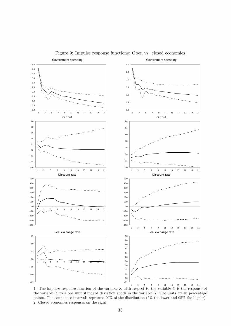
Figure 9: Impulse response functions: Open vs. closed economies

0.0

0.5

1.0

1.5

2.0

2.5

3.0

3.5

4.0

4.5

5.0

1 3 5 7 9 11 13 15 17 19 21

Government spending

0.0

0.5

1.0

1.5

2.0

2.5

3.0

1 3 5 7 9 11 13 15 17 19 21

Government spending

-0.6

-0.4

-0.2

0.0

0.2

0.4

0.6

0.8

1.0

1 3 5 7 9 11 13 15 17 19 21

Output

0.0

0.2

0.4

0.6

0.8

1.0

1.2

1.4

1 3 5 7 9 11 13 15 17 19 21

Output

-40.0

-30.0

-20.0

-10.0

0.0

10.0

20.0

30.0

40.0

50.0

60.0

1 3 5 7 9 11 13 15 17 19 21

Discount rate

-40.0

-30.0

-20.0

-10.0

0.0

10.0

20.0

30.0

40.0

50.0

60.0

1 3 5 7 9 11 13 15 17 19 21

Discount rate

-1.5

-1.0

-0.5

0.0

0.5

1.0

1.5

1 3 5 7 9 11 13 15 17 19 21

Real exchange rate

-0.2

0.0

0.2

0.4

0.6

0.8

1.0

1.2

1.4

1.6

1.8

2.0

1 3 5 7 9 11 13 15 17 19 21

Real exchange rate

1. The impulse response function of the variable X with respect to the variable Y is the response ofthe variable X to a one unit standard deviation shock in the variable Y. The units are in percentagepoints. The confidence intervals represent 90% of the distribution (5% the lower and 95% the higher)2. Closed economies responses on the right

35

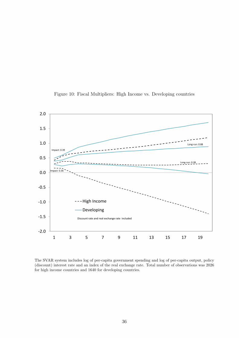
Figure 10: Fiscal Multipliers: High Income vs. Developing countries

-2.0

-1.5

-1.0

-0.5

0.0

0.5

1.0

1.5

2.0

1 3 5 7 9 11 13 15 17 19

High Income

Developing

Impact: 0.39

Impact: 0.36

Long-run: 0.88

Long-run: 0.38

Discount rate and real exchange rate included

The SVAR system includes log of per-capita government spending and log of per-capita output, policy(discount) interest rate and an index of the real exchange rate. Total number of observations was 2026for high income countries and 1640 for developing countries.

36

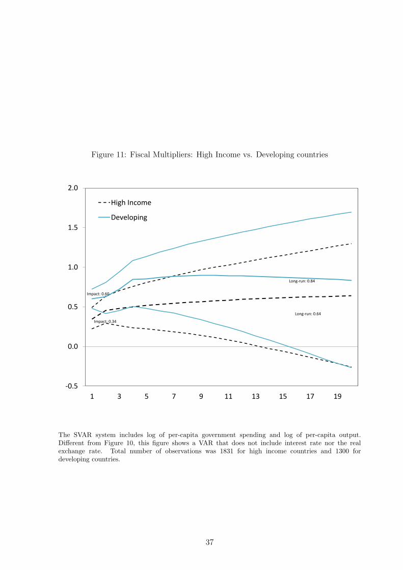
Figure 11: Fiscal Multipliers: High Income vs. Developing countries

-0.5

0.0

0.5

1.0

1.5

2.0

1 3 5 7 9 11 13 15 17 19

High Income

Developing

Impact: 0.34

Impact: 0.60

Long-run: 0.84

Long-run: 0.64

The SVAR system includes log of per-capita government spending and log of per-capita output.Different from Figure 10, this figure shows a VAR that does not include interest rate nor the realexchange rate. Total number of observations was 1831 for high income countries and 1300 fordeveloping countries.

37

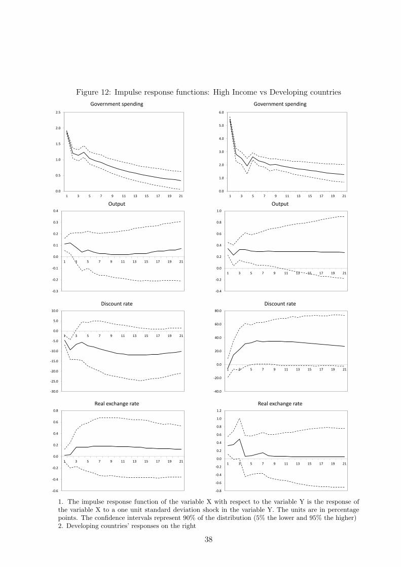
Figure 12: Impulse response functions: High Income vs Developing countries

0.0

0.5

1.0

1.5

2.0

2.5

1 3 5 7 9 11 13 15 17 19 21

Government spending

0.0

1.0

2.0

3.0

4.0

5.0

6.0

1 3 5 7 9 11 13 15 17 19 21

Government spending

-0.3

-0.2

-0.1

0.0

0.1

0.2

0.3

0.4

1 3 5 7 9 11 13 15 17 19 21

Output

-0.4

-0.2

0.0

0.2

0.4

0.6

0.8

1.0

1 3 5 7 9 11 13 15 17 19 21

Output

-30.0

-25.0

-20.0

-15.0

-10.0

-5.0

0.0

5.0

10.0

1 3 5 7 9 11 13 15 17 19 21

Discount rate

-40.0

-20.0

0.0

20.0

40.0

60.0

80.0

1 3 5 7 9 11 13 15 17 19 21

Discount rate

-0.6

-0.4

-0.2

0.0

0.2

0.4

0.6

0.8

1 3 5 7 9 11 13 15 17 19 21

Real exchange rate

-0.8

-0.6

-0.4

-0.2

0.0

0.2

0.4

0.6

0.8

1.0

1.2

1 3 5 7 9 11 13 15 17 19 21

Real exchange rate

1. The impulse response function of the variable X with respect to the variable Y is the response ofthe variable X to a one unit standard deviation shock in the variable Y. The units are in percentagepoints. The confidence intervals represent 90% of the distribution (5% the lower and 95% the higher)2. Developing countries’ responses on the right

38

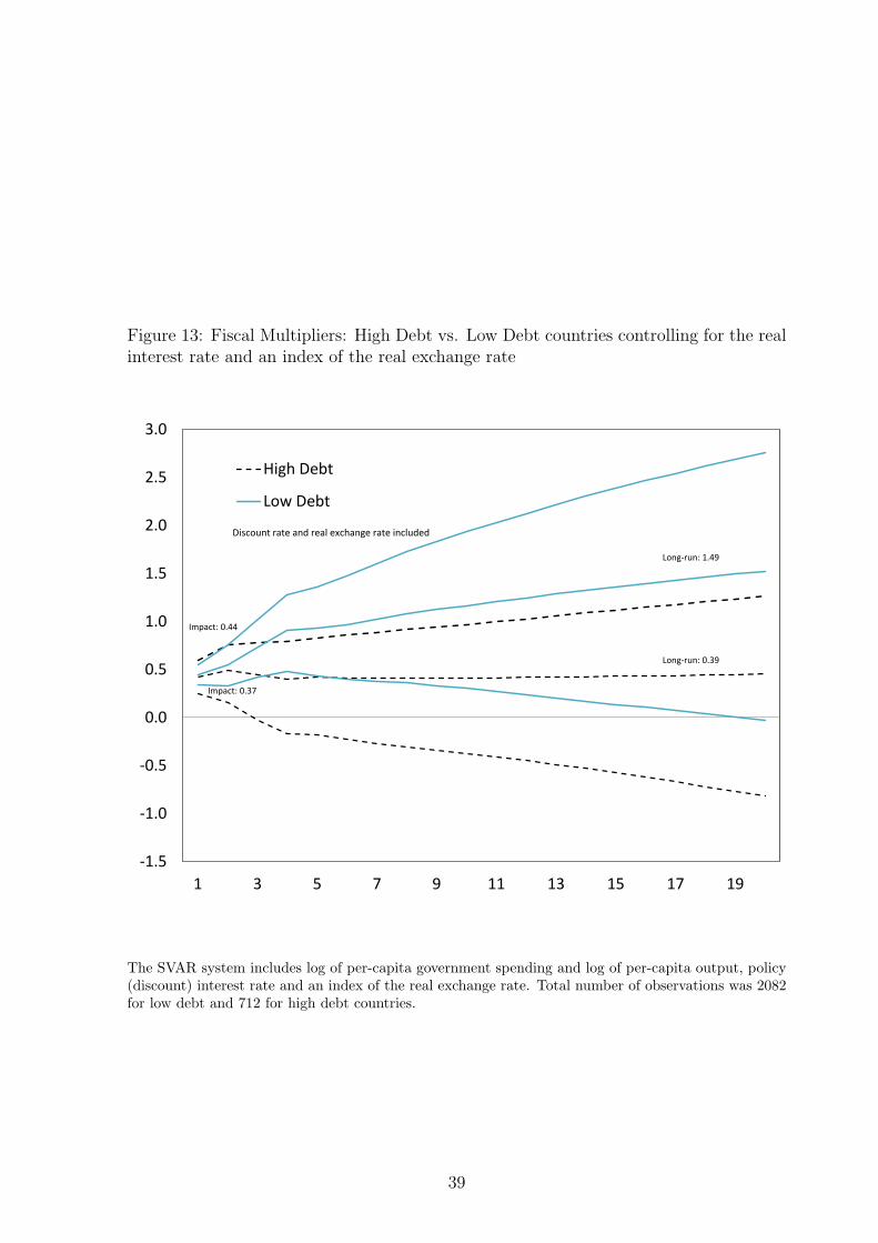
Figure 13: Fiscal Multipliers: High Debt vs. Low Debt countries controlling for the realinterest rate and an index of the real exchange rate

-1.5

-1.0

-0.5

0.0

0.5

1.0

1.5

2.0

2.5

3.0

1 3 5 7 9 11 13 15 17 19

High Debt

Low Debt

Impact: 0.44

Impact: 0.37

Long-run: 0.39

Long-run: 1.49

Discount rate and real exchange rate included

The SVAR system includes log of per-capita government spending and log of per-capita output, policy(discount) interest rate and an index of the real exchange rate. Total number of observations was 2082for low debt and 712 for high debt countries.

39

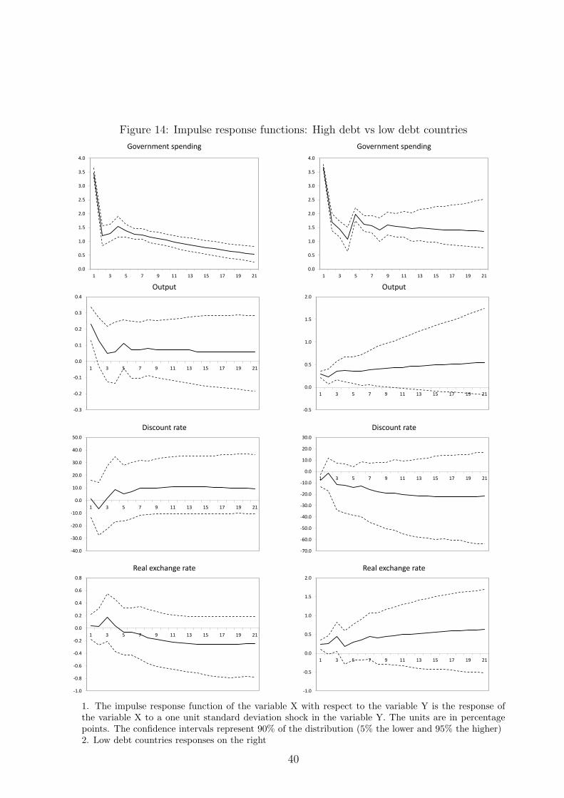
Figure 14: Impulse response functions: High debt vs low debt countries

0.0

0.5

1.0

1.5

2.0

2.5

3.0

3.5

4.0

1 3 5 7 9 11 13 15 17 19 21

Government spending

0.0

0.5

1.0

1.5

2.0

2.5

3.0

3.5

4.0

1 3 5 7 9 11 13 15 17 19 21

Government spending

-0.3

-0.2

-0.1

0.0

0.1

0.2

0.3

0.4

1 3 5 7 9 11 13 15 17 19 21

Output

-0.5

0.0

0.5

1.0

1.5

2.0

1 3 5 7 9 11 13 15 17 19 21

Output

-40.0

-30.0

-20.0

-10.0

0.0

10.0

20.0

30.0

40.0

50.0

1 3 5 7 9 11 13 15 17 19 21

Discount rate

-70.0

-60.0

-50.0

-40.0

-30.0

-20.0

-10.0

0.0

10.0

20.0

30.0

1 3 5 7 9 11 13 15 17 19 21

Discount rate

-1.0

-0.8

-0.6

-0.4

-0.2

0.0

0.2

0.4

0.6

0.8

1 3 5 7 9 11 13 15 17 19 21

Real exchange rate

-1.0

-0.5

0.0

0.5

1.0

1.5

2.0

1 3 5 7 9 11 13 15 17 19 21

Real exchange rate

1. The impulse response function of the variable X with respect to the variable Y is the response ofthe variable X to a one unit standard deviation shock in the variable Y. The units are in percentagepoints. The confidence intervals represent 90% of the distribution (5% the lower and 95% the higher)2. Low debt countries responses on the right

40

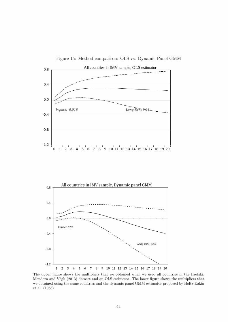
Figure 15: Method comparison: OLS vs. Dynamic Panel GMM

-1.2

-0.8

-0.4

0.0

0.4

0.8

0 1 2 3 4 5 6 7 8 9 10 11 12 13 14 15 16 17 18 19 20

Impact: -0.016 Long Run: 0.26

All countries in IMV sample, OLS estimator

-1.2

-0.8

-0.4

0.0

0.4

0.8

1 2 3 4 5 6 7 8 9 10 11 12 13 14 15 16 17 18 19 20

Impact: 0.02

Long-run: -0.40

All countries in IMV sample, Dynamic panel GMM

The upper figure shows the multipliers that we obtained when we used all countries in the Ilzetzki,Mendoza and Vegh (2013) dataset and an OLS estimator. The lower figure shows the multipliers thatwe obtained using the same countries and the dynamic panel GMM estimator proposed by Holtz-Eakinet al. (1988)

41

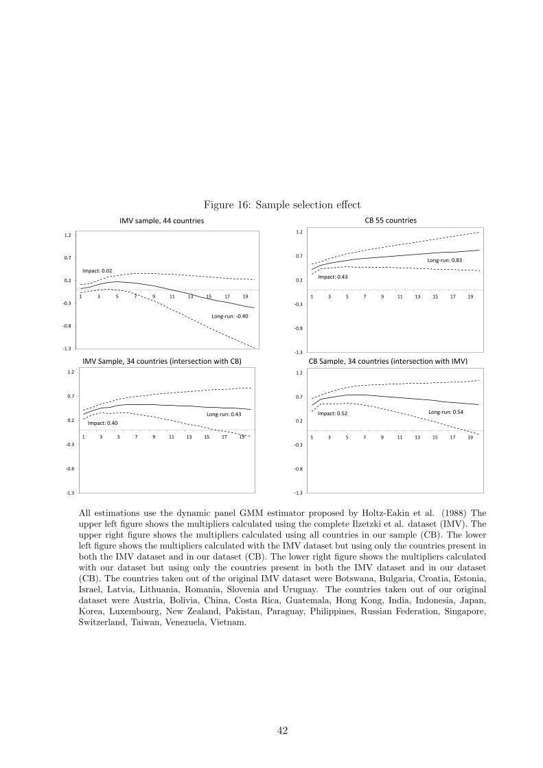
Figure 16: Sample selection effect

-1.3

-0.8

-0.3

0.2

0.7

1.2

1 3 5 7 9 11 13 15 17 19

Impact: 0.02

Long-run: -0.40

IMV sample, 44 countries

-1.3

-0.8

-0.3

0.2

0.7

1.2

1 3 5 7 9 11 13 15 17 19

Impact: 0.43

Long-run: 0.83

CB 55 countries

-1.3

-0.8

-0.3

0.2

0.7

1.2

1 3 5 7 9 11 13 15 17 19

Impact: 0.40

Long-run: 0.43

IMV Sample, 34 countries (intersection with CB)

-1.3

-0.8

-0.3

0.2

0.7

1.2

1 3 5 7 9 11 13 15 17 19

Impact: 0.52 Long-run: 0.54

CB Sample, 34 countries (intersection with IMV)

All estimations use the dynamic panel GMM estimator proposed by Holtz-Eakin et al. (1988) Theupper left figure shows the multipliers calculated using the complete Ilzetzki et al. dataset (IMV). Theupper right figure shows the multipliers calculated using all countries in our sample (CB). The lowerleft figure shows the multipliers calculated with the IMV dataset but using only the countries present inboth the IMV dataset and in our dataset (CB). The lower right figure shows the multipliers calculatedwith our dataset but using only the countries present in both the IMV dataset and in our dataset(CB). The countries taken out of the original IMV dataset were Botswana, Bulgaria, Croatia, Estonia,Israel, Latvia, Lithuania, Romania, Slovenia and Uruguay. The countries taken out of our originaldataset were Austria, Bolivia, China, Costa Rica, Guatemala, Hong Kong, India, Indonesia, Japan,Korea, Luxembourg, New Zealand, Pakistan, Paraguay, Philippines, Russian Federation, Singapore,Switzerland, Taiwan, Venezuela, Vietnam.

42

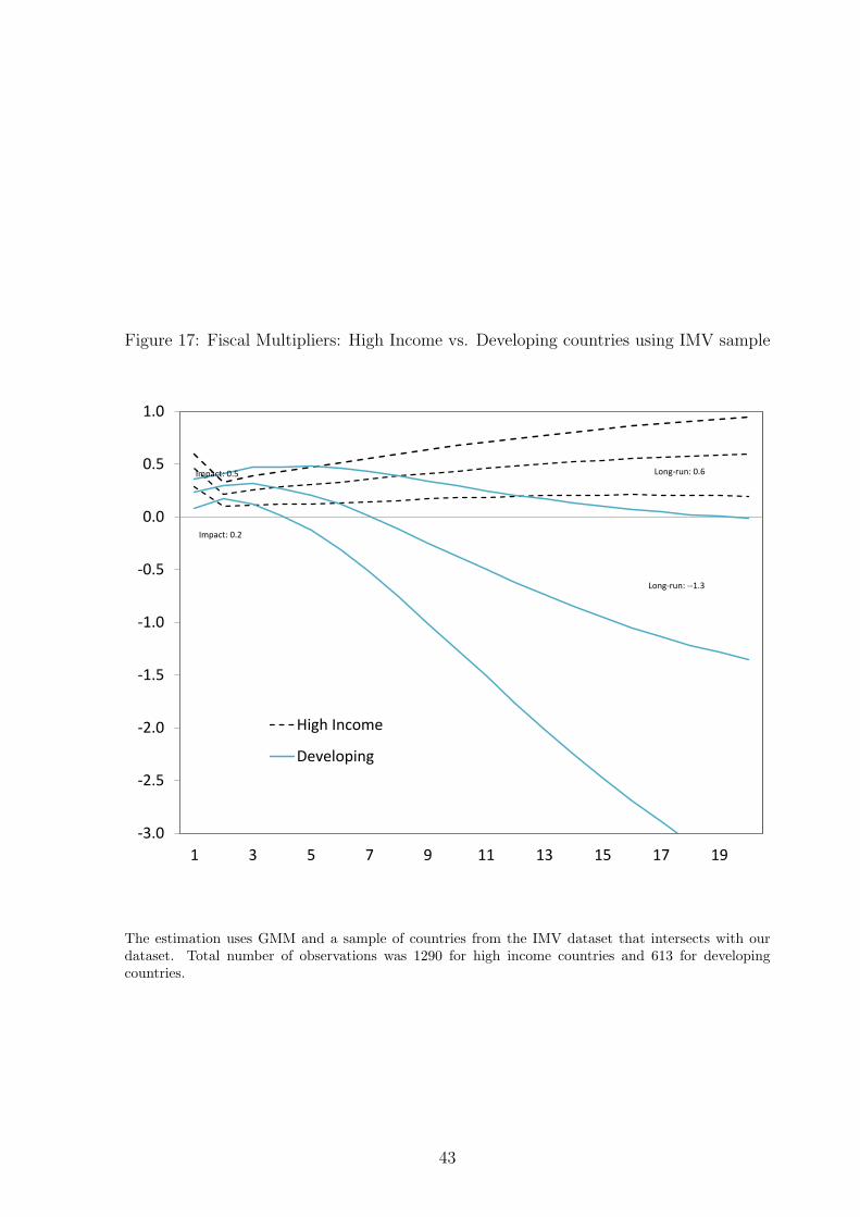
Figure 17: Fiscal Multipliers: High Income vs. Developing countries using IMV sample

-3.0

-2.5

-2.0

-1.5

-1.0

-0.5

0.0

0.5

1.0

1 3 5 7 9 11 13 15 17 19

High Income

Developing

Impact: 0.5

Impact: 0.2

Long-run: 0.6

Long-run: --1.3

The estimation uses GMM and a sample of countries from the IMV dataset that intersects with ourdataset. Total number of observations was 1290 for high income countries and 613 for developingcountries.

43

SU

PPLEM

EN

TA

RY

INFO

RM

AT

ION

:D

ATA

SO

UR

CES

AN

DT

IME

PER

IOD

S

CO

UN

TRY

VA

RIA

BLE

NA

ME

SO

UR

CE

TIM

EPER

IOD

Arg

enti

na

GD

Pat

curr

ent

pri

ces

Secre

tarı

ade

Pro

gra

macio

nEconom

ica

Min

iste

rio

de

Econom

ıay

Obra

sy

Serv

icio

sPublicos

1993q1

-2010q2

Public

consu

mpti

on

Secre

tarı

ade

Pro

gra

macio

nEconım

ica

Min

iste

rio

de

Econom

iay

Obra

sy

Serv

icio

sPublicos

1993q1

-2010q2

Pri

vate

consu

mpti

on

Secre

tarı

ade

Pro

gra

macio

nEconım

ica

Min

iste

rio

de

Econom

ıay

Obra

sy

Serv

icio

sPublicos

1993q1

-2010q2

GD

Pim

plicit

deflato

r(1

993=

100)

Inst

ituto

Nacio

nalde

Est

adıs

tica

yC

enso

s.1993q1

-2010q2

Dis

count

rate

(policy

inte

rest

rate

)IM

F1991q1

-2010q4

Realeffecti

ve

exchange

rate

IMF,B

IS1994q1

-2010q4

Em

plo

ym

ent

Inst

ituto

Nacio

nalde

Est

adıs

tica

yC

enso

s.1991q1

-2010q1

Aust

ralia

GD

Pat

curr

ent

pri

ces

Aust

ralian

Bure

au

ofSta

tist

ics

1988q1

-2010q2

Fin

alconsu

mpti

on

expendit

ure

s.Public

Aust

ralian

Bure

au

ofSta

tist

ics

1988q1

-2010q2

Fin

alconsu

mpti

on

expendit

ure

s.Pri

vate

Aust

ralian

Bure

au

ofSta

tist

ics

1988q1

-2010q2

GD

Pdeflato

r(Q

3/2005-Q

2/2006=

100)

Aust

ralian

Bure

au

ofSta

tist

ics

1988q1

-2010q2

Dis

count

rate

(policy

inte

rest

rate

)IM

F1988q1

-2010q4

Realeffecti

ve

exchange

rate

IMF,B

IS1988q1

-2010q4

Em

plo

ym

ent

(Thousa

nds)

Aust

ralian

Bure

au

ofSta

tist

ics

1988q1

-2010q3

Aust

ria

GD

Pat

curr

ent

pri

ces

Sta

tist

ikA

ust

ria

1988q1

-2010q2

Govern

ment

spendin

gIS

FD

ATA

1988q1

-2010q2

Fin

alconsu

mpti

on

expendit

ure

Sta

tist

ikA

ust

ria

1988q1

-2010q2

GD

Pdeflato

r(2

000=

100)

Sta

tist

ikA

ust

ria

1988q1

-2010q2

Offi

cia

lin

tere

stra

teA

ust

err

eic

his

che

Nati

onalb

ank

(OeN

B)

1988q1

-2010q4

Realeffecti

ve

exchange

rate

IMF,B

IS1988q1

-2010q4

Em

plo

ym

ent

Ost

err

eic

his

ches

Inst

itute

for

Wir

tschaft

sfors

chung

1988q1

-2010q4

Belg

ium

GD

Pat

curr

ent

pri

ces

Banque

Nati

onale

de

Belg

ique

1995q1

-2010q2

Govern

ment

finalconsu

mpti

on

expendit

ure

Banque

Nati

onale

de

Belg

ique

1995q1

-2010q2

Pri

vate

finalconsu

mpti

on

expendit

ure

Banque

Nati

onale

de

Belg

ique

1995q1

-2010q2

GD

Pdeflato

r(2

005=

100)

Banque

Nati

onale

de

Belg

ique

1988q1

-2010q4

Offi

cia

lin

tere

stra

teIM

F1988q1

-1998q4

Realeffecti

ve

exchange

rate

IMF,B

IS1988q1

-2010q4

Em

plo

ym

ent

NA

.

Bolivia

GD

Pat

curr

ent

pri

ces

Inst

ituto

Nacio

nalde

Est

adıs

tica/B

anco

Centr

alde

Bolivia

1993q2

-2010q2

Public

consu

mpti

on

Inst

ituto

Nacio

nalde

Est

adıs

tica/B

anco

Centr

alde

Bolivia

1993q2

-2010q2

Pri

vate

consu

mpti

on

Inst

ituto

Nacio

nalde

Est

adıs

tica/B

anco

Centr

alde

Bolivia

1993q2

-2010q2

GD

PIm

plicit

Deflato

r(1

990=

100)

Inst

ituto

Nacio

nalde

Est

adıs

tica/B

anco

Centr

alde

Bolivia

1988q1

-2010q2

Dis

count

rate

(policy

inte

rest

rate

)W

eekly

Bank

Report

s.B

anco

Centr

alde

Bolivia

,IM

F1988q1

-2010q4

Realeffecti

ve

exchange

rate

IMF,B

IS1988q1

-2010q4

Em

plo

ym

ent

NA

.

Bra

zil

GD

Pat

curr

ent

pri

ces

Fundacao

Inst

ituto

Bra

sile

iro

de

Geogra

fia

eEst

ati

stic

a.

1990q2

-2010q2

Govern

ment

consu

mpti

on

Fundacao

Inst

ituto

Bra

sile

iro

de

Geogra

fia

eEst

ati

stic

a.

1994q1

-2010q2

Pri

vate

consu

mpti

on

Fundacao

Inst

ituto

Bra

sile

iro

de

Geogra

fia

eEst

ati

stic

a.

1994q1

-2010q2

Whole

sale

Pri

ce

Index,dom

est

icsu

pply

(1994=

100)

Fundacao

Getu

lio

Varg

as

SELIC

(targ

et

rate

)B

anco

Centr

aldo

Bra

sil,

IMF

1998q1

-2010q4

44

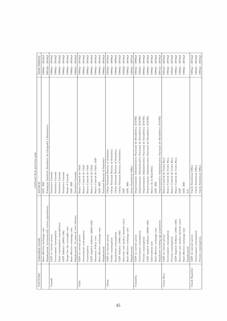
–conti

nued

from

pre

vio

us

page

CO

UN

TRY

VA

RIA

BLE

NA

ME

SO

UR

CE

TIM

EPER

IOD

Realeffecti

ve

exchange

rate

IMF,B

IS1988q1

-2010q4

Em

plo

ym

ent

(econom

ically

acti

ve

popula

tion)

Fundacao

Inst

ituto

Bra

sile

iro

de

Geogra

fia

eEst

ati

stic

a.

2001q3

-2010q3

Canadı

GD

Pat

curr

ent

pri

ces

Sta

tist

ics

Canada

1988q1

-2010q2

Govern

ment

consu

mpti

on

Sta

tist

ics

Canada

1988q1

-2010q2

Fin

alconsu

mpti

on

expendit

ure

sSta

tist

ics

Canada

1988q1

-2010q2

GD

Pdeflato

r(2

002=

100)

Sta

tist

ics

Canada

1988q1

-2010q2

Targ

et

for

the

overn

ight

rate

Bank

ofC

anada

1988q1

-2010q4

Realeffecti

ve

exchange

rate

IMF,B

IS1988q1

-2010q4

Em

plo

ym

ent:

15

years

&over

(thous)

Sta

tist

ics

Canada

1988q1

-2010q3

Chile

GD

Pat

curr

ent

pri

ces

Banco

Centr

alde

Chile

1990q1

-2010q2

Govern

ment

consu

mpti

on

Banco

Centr

alde

Chile

1996q1

-2010q2

Consu

mpti

on

Banco

Centr

alde

Chile

1996q1

-2010q2

GD

Pim

plicit

deflato

r(2

003=

100)

Banco

Centr

alde

Chile

1988q1

-2010q4

Moneta

ryPolicy

rate

Banco

Centr

alde

Chile,IM

F1988q1

-2010q4

Realeffecti

ve

exchange

rate

IMF,B

IS1988q1

-2010q4

Em

plo

ym

ent

Nati

onalB

ure

au

ofSta

tist

ics

1988q1

-2010q4

Chin

aG

DP

at

curr

ent

pri

ces

Chin

aN

ati

onalB

ure

au

ofSta

tist

ics.

1992q1

-2010q3

Public

consu

mpti

on

Chin

aN

ati

onalB

ure

au

ofSta

tist

ics.

1988q1

-2009q4

Resi

denti

alconsu

mpti

on

Chin

aN

ati

onalB

ure

au

ofSta

tist

ics.

1988q1

-2009q4

GD

Pdeflato

r(1

990=

100)

Chin

aN

ati

onalB

ure

au

ofSta

tist

ics.

1988q1

-2010q2

Dis

count

rate

(policy

inte

rest

rate

)IM

F1992q2

-2010q4

Realeffecti

ve

exchange

rate

IMF,B

IS1988q1

-2010q4

Em

plo

ym

ent

Sta

teSta

tist

icalO

ffice

1988q1

-2007q4

Colo

mbia

GD

Pat

curr

ent

pri

ces

Depart

am

ento

Adm

inis

trati

vo

Nacio

nalde

Est

adıs

tica

(DA

NE)

1994q1

-2009q4

Govern

ment

consu

mpti

on

Depart

am

ento

Adm

inis

trati

vo

Nacio

nalde

Est

adıs

tica

(DA

NE)

1994q1

-2009q4

Pri

vate

consu

mpti

on

Depart

am

ento

Adm

inis

trati

vo

Nacio

nalde

Est

adıs

tica

(DA

NE)

2000q1

-2010q2

GD

Pim

plicit

deflato

r(2

000=

100)

Depart

am

ento

Adm

inis

trati

vo

Nacio

nalde

Est

adıs

tica

(DA

NE)

1988q1

-2010q2

Inte

rventi

on

rate

Banco

de

laR

epublica

1988q1

-2010q4

Realeffecti

ve

exchange

rate

IMF,B

IS1988q1

-2010q4

Em

plo

yed

work

ing

age

popula

tion

Depart

am

ento

Adm

inis

trati

vo

Nacio

nalde

Est

adıs

tica

(DA

NE)

2001q1

-2010q4

Cost

aR

ica

GD

Pat

curr

ent

pri

ces

Banco

Centr

alde

Cost

aR

ica

1991q1

-2010q2

Govern

ment

consu

mpti

on

Banco

Centr

alde

Cost

aR

ica.

1994q1

-2010q2

Pri

vate

consu

mpti

on

Banco

Centr

alde

Cost

aR

ica

1994q1

-2010q2

GD

PIm

plicit

Deflato

r(1

991=

100)

Banco

Centr

alde

Cost

aR

ica.

1988q1

-2010q2

Dis

count

rate

(policy

inte

rest

rate

)IM

F1988q1

-2010q4

Realeffecti

ve

exchange

rate

IMF,B

IS1988q1

-2010q4

Em

plo

ym

ent

NA

.

Czech

Republic

GD

Pat

curr

ent

pri

ces

Czech

Sta

tist

icalO

ffice

1995q1

-2010q2

Govern

ment

consu

mpti

on

Czech

Sta

tist

icalO

ffice

1995q1

-2010q2

Pri

vate

consu

mpti

on

Czech

Sta

tist

icalO

ffice

1995q1

-2010q2

45

–conti

nued

from

pre

vio

us

page

CO

UN

TRY

VA

RIA

BLE

NA

ME

SO

UR

CE

TIM

EPER

IOD

GD

PIm

plicit

Deflato

rC

zech

Sta

tist

icalO

ffice

1988q1

-2010q2

Dis

count

rate

(policy

inte

rest

rate

)IM

F1993q1

-2010q4

Realeffecti

ve

exchange

rate

IMF,B

IS1990q1

-2010q4

Em

plo

ym

ent

NA

.

Denm

ark

GD

Pat

curr

ent

pri

ces

Danm

ark

sSta

tist

ik1990q1

-2010q2

Govern

ment

consu

mpti

on

Danm

ark

sSta

tist

ik1990q1

-2010q2

Pri

vate

consu

mpti

on

Danm

ark

sSta

tist

ik1990q1

-2010q2

GD

PIm

plicit

Deflato

r(1

991=

100)

Danm

ark

sSta

tist

ik1988q1

-2010q2

Dis

count

rate

(policy

inte

rest

rate

)IM

F1988q1

-2010q4

Realeffecti

ve

exchange

rate

IMF,B

IS1988q1

-2010q4

Em

plo

ym

ent

NA

.

Ecuador

GD

Pat

curr

ent

pri

ces

Banco

Centr

aldelEcuador

1990q1

-2010q2

Govern

ment

consu

mpti

on

Banco

Centr

aldelEcuador

1990q1

-2010q2

Pri

vate

consu

mpti

on

Banco

Centr

aldelEcuador

1990q1

-2010q2

GD

Pdeflato

rB

anco

Centr

aldelEcuador

1988q1

-2010q2

Basi

ccentr

alB

ank

Rate

(policy

inte

rest

rate

)IM

F1988q1

-2010q4

Realeffecti

ve

exchange

rate

IMF,B

IS1988q1

-2010q4

Em

plo

ym

ent:

glo

baloccupati

on

rate

(%)

Banco

Centr

aldelEcuador

1998q3

-2008q4

ElSalv

ador

GD

Pat

curr

ent

pri

ces

Banco

Centr

alde

Rese

rva

delSalv

ador

1990q1

-2010q2

Public

consu

mpti

on

Banco

Centr

alde

Rese

rva

delSalv

ador

1993q2

-2009q4

Pri

vate

consu

mpti

on

Banco

Centr

alde

Rese

rva

delSalv

ador

1993q2

-2009q4

GD

PD

eflato

rH

aver

Analy

tics

1988q1

-2010q2

Dis

count

rate

(policy

inte

rest

rate

)IM

F1995q1

-2010q4

Realeffecti

ve

exchange

rate

NA

Em

plo

ym

ent

NA

.

Fin

land

GD

Pat

curr

ent

pri

ces

Tilast

okesk

us

(Sta

tist

ics

Fin

land)

1988q1

-2010q2

Fin

alconsu

mpti

on

expendit

ure

.Pri

vate

Tilast

okesk

us

(Sta

tist

ics

Fin

land)

1988q1

-2010q2

Fin

alconsu

mpti

on

expendit

ure

.G

overn

ment

Tilast

okesk

us

(Sta

tist

ics

Fin

land)

1988q1

-2010q2

GD

Pdeflato

r(2

000=

100)

Tilast

okesk

us

(Sta

tist

ics

Fin

land)

1988q1

-2010q2

Offi

cia

lin

tere

stra

te(E

nd

ofPeri

od)

Bank

ofFin

land

1988q1

-2010q4

Realeffecti

ve

exchange

rate

IMF,B

IS1988q1

-2010q4

Em

plo

ym

ent

NA

Fra

nce

GD

Pat

curr

ent

pri

ces

Inst

itut

Nati

onalde

laSta

tist

ique

et

des

Etu

des

Econom

iques.

1988q1

-2010q2

Fin

alconsu

mpti

on

expendit

ure

s.Public

Inst

itut

Nati

onalde

laSta

tist

ique

et

des

Etu

des

Econom

iques.

1988q1

-2010q2

Fin

alconsu

mpti

on

expendit

ure

s.Pri

vate

Inst

itut

Nati

onalde

laSta

tist

ique

et

des

Etu

des

Econom

iques.

1988q1

-2010q2

GD

Pdeflato

r(2

000=

100)

Inst

itut

Nati

onalde

laSta

tist

ique

et

des

Etu

des

Econom

iques.

1988q1

-2010q2

Offi

cia

lin

tere

stra

tes

Banque

de

Fra

nce

1988q1

-2010q2

Realeffecti

ve

exchange

rate

IMF,B

IS1988q1

-2010q2

Em

plo

ym

ent

Inst

itut

Nati

onalde

laSta

tist

ique

et

des

Etu

des

Econom

iques.

1995q1

-2010q2

Germ

any

GD

Pat

curr

ent

pri

ces

Deuts

che

Bundesb

ank

1988q1

-2010q2

46

–conti

nued

from

pre

vio

us

page

CO

UN

TRY

VA

RIA

BLE

NA

ME

SO

UR

CE

TIM

EPER

IOD

Fin

alconsu

mpti

on

expendit

ure

s.Public

Deuts

che

Bundesb

ank

1988q1

-2010q2

Fin

alconsu

mpti

on

expendit

ure

s.Pri

vate

Deuts

che

Bundesb

ank

1988q1

-2010q2

GD

Pdeflato

r(2

000=

100)

Deuts

che

Bundesb

ank

1988q1

-2010q2

Offi

cia

lin

tere

stra

tes

Deuts

che

Bundesb

ank

1988q1

-2010q2

Realeffecti

ve

exchange

rate

IMF,B

IS1988q1

-2010q2

Em

plo

ym

ent

(Thousa

nds)

Deuts

che

Bundesb

ank

1988q1

-2010q2

Gre

ece

GD

Pat

curr

ent

pri

ces

Nati

onalSta

tist

icalServ

ice

ofG

reece

2000q1

-2010q2

Public

consu

mpti

on

Nati

onalSta

tist

icalServ

ice

ofG

reece

2000q1

-2010q2

Pri

vate

consu

mpti

on

Nati

onalSta

tist

icalServ

ice

ofG

reece

2000q1

-2010q2

GD

Pdeflato

r(2

000=

100).

Quart

erl

yN

ati

onalSta

tist

icalServ

ice

ofG

reece

2000q1

-2010q2

Dis

count

rate

(policy

inte

rest

rate

)IM

F1988q1

-2000q4

Realeffecti

ve

exchange

rate

IMF,B

IS1988q1

-2010q4

Em

plo

ym

ent

NA

Guate

mala

GD

Pat

curr

ent

pri

ces

Banco

de

Guate

mala

2001q1

-2009q4

Govern

ment

consu

mpti

on

Banco

de

Guate

mala

2001q1

-2009q4

Pri

vate

consu

mpti

on

Banco

de

Guate

mala

2001q1

-2009q4

GD

Pdeflato

rB

anco

de

Guate

mala

1988q1

-2010q2

Dis

count

rate

(policy

inte

rest

rate

)IM

F1988q1

-1992q2

Realeffecti

ve

exchange

rate

NA

Em

plo

ym

ent

NA

Hong

Kong

GD

Pat

curr

ent

pri

ces

HK

Censu

sand

Sta

tist

ics

Depart

ment

1988q1

-2010q3

Govern

ment

consu

mpti

on

expendit

ure

HK

Censu

sand

Sta

tist

ics

Depart

ment

1988q1

-2010q3

Pri

vate

consu

mpti

on

expendit

ure

HK

Censu

sand

Sta

tist

ics

Depart

ment

1988q1

-2010q3

GD

Pdeflato

r(2

000=

100)

HK

Censu

sand

Sta

tist

ics

Depart

ment

1988q1

-2010q2

Dis

count

rate

(policy

inte

rest

rate

)IM

F1988q1

-2010q4

Realeffecti

ve

exchange

rate

IMF,B

IS1988q1

-2010q4

Em

plo

ym

ent

NA

Hungary

GD

Pat

curr

ent

pri

ces

Centr

alSta

tist

icalO

ffice

1995q1

-2010q2

Govern

ment

consu

mpti

on

expendit

ure

Centr

alSta

tist

icalO

ffice

1995q1

-2010q2

Pri

vate

consu

mpti

on

expendit

ure

Centr

alSta

tist

icalO

ffice

1995q1

-2010q2

GD

Pdeflato

rC

entr

alSta

tist

icalO

ffice

(Haver

Analy

tics)

1995q1

-2010q2

Dis

count

rate

(policy

inte

rest

rate

)IM

F1990q1

-2010q4

Realeffecti

ve

exchange

rate

IMF,B

IS1988q1

-2010q4

Em

plo

ym

ent

NA

Icela

nd

GD

Pat

curr

ent

pri

ces

Sta

tist

ics

Icela

nd

1997q1

-2010q2

Govern

ment

finalconsu

mpti

on

Sta

tist

ics

Icela

nd

1997q1

-2010q2

Pri

vate

finalconsu

mpti

on

Sta

tist

ics

Icela

nd

1997q1

-2010q2

GD

Pim

plicit

pri

ce

deflato

r(2

000=

100)

Sta

tist

ics

Icela

nd

1988q1

-2010q2

Inte

rbank

Offere

dR

ate

(REIB

OR

)C

entr

alB

ank

ofIc

ela

nd

1994q2

-2010q4

Realeffecti

ve

exchange

rate

IMF,B

IS1988q1

-2010q4

47

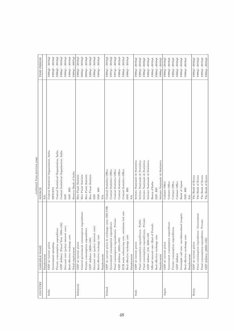
–conti

nued

from

pre

vio

us

page

CO

UN

TRY

VA

RIA

BLE

NA

ME

SO

UR

CE

TIM

EPER

IOD

Em

plo

ym

ent

NA

.

India

GD

Pat

curr

ent

pri

ces

Centr

alSta

tist

icalO

rganiz

ati

on,In

dia

.1996q2

-2010q2

Govern

ment

spendin

gIS

FD

ATA

1996q2

-2010q2

Pri

vate

consu

mpti

on

expendit

ure

Centr

alSta

tist

icalO

rganiz

ati

on,In

dia

.1996q2

-2010q2

GD

Pdeflato

r(F

iscalYear

1999=

100)

Centr

alSta

tist

icalO

rganiz

ati

on,In

dia

.1988q1

-2010q4

Dis

count

rate

(policy

inte

rest

rate

)IM

F1988q1

-2010q4

Realeffecti

ve

exchange

rate

IMF,B

IS1988q1

-2010q4

Tota

lem

plo

ym

ent

Rese

rve

Bank

ofIn

dia

1988q1

-2007q2

Indonesi

aG

DP

at

curr

ent

pri

ces

Bir

oPusa

tSta

tist

ic1988q1

-2010q3

Genera

lgovern

ment

consu

mpti

on

expendit

ure

Bir

oPusa

tSta

tist

ic2000q1

-2010q3

Pri

vate

consu

mpti

on

expendit

ure

Bir

oPusa

tSta

tist

ic2000q1

-2010q3

GD

Pdeflato

r(2

000=

100)

Bir

oPusa

tSta

tist

ic1988q1

-2010q3

Dis

count

rate

(policy

inte

rest

rate

)IM

F1990q1

-2010q4

Realeffecti

ve

exchange

rate

IMF,B

IS1994q1

-2010q4

Em

plo

ym

ent

NA

.

Irela

nd

GD

Pat

curr

ent

pri

ces

&exchange

rate

s(M

il.U

S$)

Centr

alSta

tist

ics

Offi

ce

1988q1

-2010q2

Govern

ment

consu

mpti

on

expendit

ure

Centr

alSta

tist

ics

Offi

ce

1997q1

-2010q2

Fin

alconsu

mpti

on

expendit

ure

s.Pri

vate

Centr

alSta

tist

ics

Offi

ce

1997q1

-2010q2

GD

Pdeflato

r(2

005=

100)

Centr

alSta

tist

ics

Offi

ce

1988q1

-2010q4

EC

Bm

ain

refinancin

gra

te:

min

imum

bid

rate

Centr

alSta

tist

ics

Offi

ce

1988q1

-2010q4

Realeffecti

ve

exchange

rate

IMF,B

IS1988q1

-2010q4

Em

plo

ym

ent

NA

.

Italy

GD

Pat

curr

ent

pri

ces

Isti

tuto

Nazio

nale

diSta

tist

ica

1988q1

-2010q2

Fin

alconsu

mpti

on

expendit

ure

s.Public

Isti

tuto

Nazio

nale

diSta

tist

ica

1988q1

-2010q2

Fin

alconsu

mpti

on

expendit

ure

s.Pri

vate

Isti

tuto

Nazio

nale

diSta

tist

ica

1988q1

-2010q2

GD

Pdeflato

r(S

A,2000=

100

Isti

tuto

Nazio

nale

diSta

tist

ica

1988q1

-2010q2

Offi

cia

lin

tere

stra

te(E

nd

ofPeri

od)

Banca

d’Ita

lia

1988q1

-2010q4

Realeffecti

ve

exchange

rate

IMF,B

IS1988q1

-2010q4

Em

plo

ym

ent

Isti

tuto

Nazio

nale

diSta

tist

ica

1988q1

-2010q2

Japan

GD

Pat

curr

ent

pri

ces

Cabin

et

Offi

ce

1988q1

-2010q2

Govern

ment

consu

mpti

on

expendit

ure

Cabin

et

Offi

ce

1988q1

-2010q2

Pri

vate

consu

mpti

on

expendit

ure

sC

abin

et

Offi

ce

1988q1

-2010q2

GD

Pdeflato

rC

abin

et

Offi

ce

1988q1

-2010q2

Overn

ight

call

rate

:uncollate

ralized

(targ

et)

Bank

ofJapan

1988q1

-2010q4

Realeffecti

ve

exchange

rate

IMF,B

IS1988q1

-2010q4

Em

plo

ym

ent

NA

.

Kore

aG

DP

at

curr

ent

pri

ces

The

Bank

ofK

ore

a1988q1

-2010q2

Fin

alconsu

mpti

on

expendit

ure

.G

overn

ment

The

Bank

ofK

ore

a1988q1

-2010q2

Fin

alconsu

mpti

on

expendit

ure

.Pri

vate

The

Bank

ofK

ore

a1988q1

-2010q2

GD

Pdeflato

r(2

000=

100)

The

Bank

ofK

ore

a1988q1

-2010q2

48

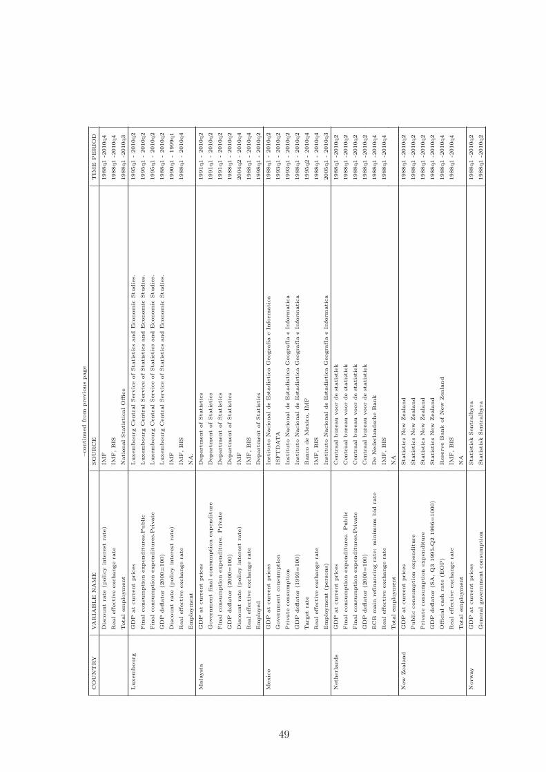
–conti

nued

from

pre

vio

us

page

CO

UN

TRY

VA

RIA

BLE

NA

ME

SO

UR

CE

TIM

EPER

IOD

Dis

count

rate

(policy

inte

rest

rate

)IM

F1988q1

-2010q4

Realeffecti

ve

exchange

rate

IMF,B

IS1988q1

-2010q4

Tota

lem

plo

ym

ent

Nati

onalSta

tist

icalO

ffice

1988q1

-2010q3

Luxem

bourg

GD

Pat

curr

ent

pri

ces

Luxem

bourg

Centr

alServ

ice

ofSta

tist

ics

and

Econom

icStu

die

s.1995q1

-2010q2

Fin

alconsu

mpti

on

expendit

ure

s.Public

Luxem

bourg

Centr

alServ

ice

ofSta

tist

ics

and

Econom

icStu

die

s.1995q1

-2010q2

Fin

alconsu

mpti

on

expendit

ure

s.Pri

vate

Luxem

bourg

Centr

alServ

ice

ofSta

tist

ics

and

Econom

icStu

die

s.1995q1

-2010q2

GD

Pdeflato

r(2

000=

100)

Luxem

bourg

Centr

alServ

ice

ofSta

tist

ics

and

Econom

icStu

die

s.1988q1

-2010q2

Dis

count

rate

(policy

inte

rest

rate

)IM

F1990q1

-1999q1

Realeffecti

ve

exchange

rate

IMF,B

IS1988q1

-2010q4

Em

plo

ym

ent

NA

.

Mala

ysi

aG

DP

at

curr

ent

pri

ces

Depart

ment

ofSta

tist

ics

1991q1

-2010q2

Govern

ment

finalconsu

mpti

on

expendit

ure

Depart

ment

ofSta

tist

ics

1991q1

-2010q2

Fin

alconsu

mpti

on

expendit

ure

.Pri

vate

Depart

ment

ofSta

tist

ics

1991q1

-2010q2

GD

Pdeflato

r(2

000=

100)

Depart

ment

ofSta

tist

ics

1988q1

-2010q2

Dis

count

rate

(policy

inte

rest

rate

)IM

F2004q2

-2010q4

Realeffecti

ve

exchange

rate

IMF,B

IS1988q1

-2010q4

Em

plo

yed

Depart

ment

ofSta

tist

ics

1998q1

-2010q2

Mexic

oG

DP

at

curr

ent

pri

ces

Inst

ituto

Nacio

nalde

Est

adis

tica

Geogra

fia

eIn

form

ati

ca

1988q1

-2010q2

Govern

ment

consu

mpti

on

ISFT

DATA

1993q1

-2010q2

Pri

vate

consu

mpti

on

Inst

ituto

Nacio

nalde

Est

adis

tica

Geogra

fIa

eIn

form

ati

ca

1993q1

-2010q2

GD

Pdeflato

r(1

993=

100)

Inst

ituto

Nacio

nalde

Est

adis

tica

Geogra

fIa

eIn

form

ati

ca

1988q1

-2010q2

Targ

et

rate

Banco

de

Mexic

o,IM

F1995q2

-2010q4

Realeffecti

ve

exchange

rate

IMF,B

IS1988q1

-2010q4

Em

plo

ym

ent

(pers

ons)

Inst

ituto

Nacio

nalde

Est

adis

tica

Geogra

fIa

eIn

form

ati

ca

2005q1

-2010q3

Neth

erl

ands

GD

Pat

curr

ent

pri

ces

Centr

aalbure

au

voor

de

stati

stie

k1988q1

-2010q2

Fin

alconsu

mpti

on

expendit

ure

s.Public

Centr

aalbure

au

voor

de

stati

stie

k1988q1

-2010q2

Fin

alconsu

mpti

on

expendit

ure

s.Pri

vate

Centr

aalbure

au

voor

de

stati

stie

k1988q1

-2010q2

GD

Pdeflato

r(2

000=

100)

Centr

aalbure

au

voor

de

stati

stie

k1988q1

-2010q2

EC

Bm

ain

refinancin

gra

te:

min

imum

bid

rate

De

Nederl

andsc

he

Bank

1988q1

-2010q4

Realeffecti

ve

exchange

rate

IMF,B

IS1988q1

-2010q4

Tota

lem

plo

ym

ent

NA

New

Zeala

nd

GD

Pat

curr

ent

pri

ces

Sta

tist

ics

New

Zeala

nd

1988q1

-2010q2

Public

consu

mpti

on

expendit

ure

Sta

tist

ics

New

Zeala

nd

1988q1

-2010q2

Pri

vate

consu

mpti

on

expendit

ure

Sta

tist

ics

New

Zeala

nd

1988q1

-2010q2

GD

Pdeflato

r(S

A,Q

31995-Q

21996=

1000)

Sta

tist

ics

New

Zeala

nd

1988q1

-2010q2

Offi

cia

lcash

rate

(EO

P)

Rese

rve

Bank

ofN

ew

Zeala

nd

1988q1

-2010q4

Realeffecti

ve

exchange

rate

IMF,B

IS1988q1

-2010q4

Tota

lem

plo

ym

ent

NA

Norw

ay

GD

Pat

curr

ent

pri

ces

Sta

tist

isk

Sentr

alb

yra

1988q1

-2010q2

Genera

lgovern

ment

consu

mpti

on

Sta

tist

isk

Sentr

alb

yra

1988q1

-2010q2

49

–conti

nued

from

pre

vio

us

page

CO

UN

TRY

VA

RIA

BLE

NA

ME

SO

UR

CE

TIM

EPER

IOD

Pri

vate

consu

mpti

on

Sta

tist

isk

Sentr

alb

yra

1988q1

-2010q2

GD

Pdeflato

r(2

005=

100)

Sta

tist

isk

Sentr

alb

yra

1988q1

-2010q2

Sig

ht

deposi

tra

teN

org

es

Bank

1988q1

-2010q4

Realeffecti

ve

exchange

rate

IMF,B

IS1988q1

-2010q4

Tota

lem

plo

ym

ent

NA

Pakis

tan

GD

Pat

curr

ent

pri

ces

Federa

lB

ure

au

ofSta

tist

ics

1988q4

-2010q2

Genera

lgovern

ment

Federa

lB

ure

au

ofSta

tist

ics

1998q3

-2010q2

Tota

lconsu

mpti

on.

Pri

vate

Federa

lB

ure

au

ofSta

tist

ics

1998q3

-2010q2

GD

Pdeflato

r(F

iscalyear

2000=

100)

Federa

lB

ure

au

ofSta

tist

ics

1988q1

-2010q4

Dis

count

rate

(policy

inte

rest

rate

)IM

F1988q1

-2010q4

Realeffecti

ve

exchange

rate

IMF,B

IS1988q1

-2010q4

Em

plo

ym

ent

(10

Years

and

over)

Federa

lB

ure

au

ofSta

tist

ics

1989q3

-2009q2

Para

guay

GD

Pat

curr

ent

pri

ces

Banco

Centr

aldelPara

guay

1994q1

-2010q2

Govern

ment

consu

mpti

on

Banco

Centr

aldelPara

guay

1994q1

-2010q2

Pri

vate

consu

mpti

on

Banco

Centr

aldelPara

guay

1994q1

-2010q2

GD

PIm

plicit

Deflato

r(1

982=

100)

Banco

Centr

aldelPara

guay

1988q1

-2010q2

Dis

count

rate

(policy

inte

rest

rate

)IM

F1989q4

-2010q4

Realeffecti

ve

exchange

rate

IMF,B

IS1988q1

-2010q4

Em

plo

ym

ent

NA

.

Peru

GD

Pat

curr

ent

pri

ces

Min

iste

rio

de

Econom

iay

Obra

sy

Serv

icio

sPublicos

(Haver

analy

tics)

1989q1

-2010q2

Public

consu

mpti

on

Min

iste

rio

de

Econom

iay

Obra

sy

Serv

icio

sPublicos

(Haver

analy

tics)

1992q3

-2010q2

Pri

vate

consu

mpti

on

Min

iste

rio

de

Econom

iay

Obra

sy

Serv

icio

sPublicos

(Haver

analy

tics)

1992q3

-2010q2

GD

PIm

plicit

Deflato

r(1

994=

100)

Min

iste

rio

de

Econom

iay

Obra

sy

Serv

icio

sPublicos

(Haver

analy

tics)

1988q1

-2010q2

Refe

rence

rate

(policy

inte

rest

rate

)IM

F1991q3

-2010q4

Realeffecti

ve

exchange

rate

IMF,B

IS1994q1

-2010q4

Em

plo

yed:

Metr

opolita

nLim

aB

anco

Centr

alde

Rese

rva

delPeru

2001q2

-2010q3

Philip

pin

es

GD

Pat

curr

ent

pri

ces

Nati

onalEconom

icand

Develo

pm

ent

Auth

ori

ty1988q1

-2010q2

Govern

ment

consu

mpti

on

expendit

ure

Nati

onalEconom

icand

Develo

pm

ent

Auth

ori

ty1991q3

-2010q2

Pri

vate

consu

mpti

on

Nati

onalEconom

icand

Develo

pm

ent

Auth

ori

ty1991q3

-2010q2

Gro

ssdom

est

icpro

duct

deflato

r(1

985=

100)

Nati

onalEconom

icand

Develo

pm

ent

Auth

ori

ty1988q1

-2010q2

Dis

count

rate

(policy

inte

rest

rate

)IM

F1988q1

-2010q4

Realeffecti

ve

exchange

rate

IMF,B

IS1988q1

-2010q4

Em

plo

yed

Nati

onalSta

tist

ics

Offi

ce

1990q4

-2010q3

Pola

nd

GD

Pat

curr

ent

pri

ces

Centr

alSta

tist

icalO

ffice

1995q1

-2010q2

Govern

ment

consu

mpti

on

Centr

alSta

tist

icalO

ffice

1995q1

-2010q2

Pri

vate

consu

mpti

on

Centr

alSta

tist

icalO

ffice

1995q1

-2010q2

GD

Pdeflato

rC

entr

alSta

tist

icalO

ffice

(Haver

Analy

tics)

1995q1

-2010q2

Dis

count

rate

(policy

inte

rest

rate

)IM

F1990q2

-2010q4

Realeffecti

ve

exchange

rate

IMF,B

IS1988q1

-2010q4

Em

plo

ym

ent

Centr

alSta

tist

icalO

ffice

1992q2

-2010q2

50

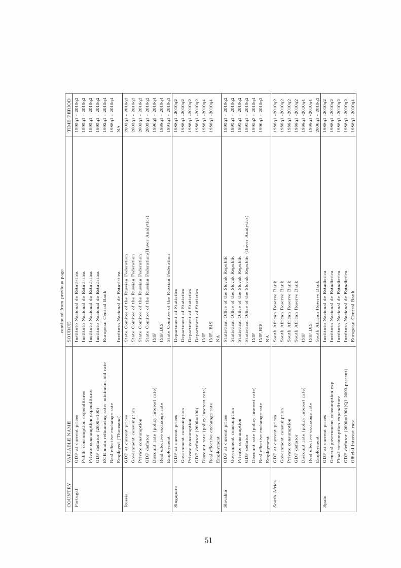
–conti

nued

from

pre

vio

us

page

CO

UN

TRY

VA

RIA

BLE

NA

ME

SO

UR

CE

TIM

EPER

IOD

Port

ugal

GD

Pat

curr

ent

pri

ces

Inst

ituto

Nacio

nalde

Est

ati

stic

a1995q1

-2010q2

Public

consu

mpti

on

expendit

ure

sIn

stit

uto

Nacio

nalde

Est

ati

stic

a1995q1

-2010q2

Pri

vate

consu

mpti

on

expendit

ure

sIn

stit

uto

Nacio

nalde

Est

ati

stic

a1995q1

-2010q2

GD

Pdeflato

r(2

000=

100)

Inst

ituto

Nacio

nalde

Est

ati

stic

a1995q1

-2010q2

EC

Bm

ain

refinancin

gra

te:

min

imum

bid

rate

Euro

pean

Centr

alB

ank

1992q1

-2010q4

Realeffecti

ve

exchange

rate

1988q1

-2010q4

Em

plo

yed

(Thousa

nd)

Inst

ituto

Nacio

nalde

Est

ati

stic

aN

A

Russ

iaG

DP

at

curr

ent

pri

ces

Sta

teC

om

itee

ofth

eR

uss

ian

Federa

tion

2003q1

-2010q2

Govern

ment

consu

mpti

on

Sta

teC

om

itee

ofth

eR

uss

ian

Federa

tion

2003q1

-2010q2

Pri

vate

consu

mpti

on

Sta

teC

om

itee

ofth

eR

uss

ian

Federa

tion

2003q1

-2010q2

GD

Pdeflato

rSta

teC

om

itee

ofth

eR

uss

ian

Federa

tion(H

aver

Analy

tics)

2003q1

-2010q2

Dis

count

rate

(policy

inte

rest

rate

)IM

F1996q3

-2010q4

Realeffecti

ve

exchange

rate

IMF,B

IS1988q1

-2010q4

Em

plo

ym

ent

Sta

teC

om

itee

ofth

eR

uss

ian

Federa

tion

1991q1

-2010q3

Sin

gapore

GD

Pat

curr

ent

pri

ces

Depart

ment

ofSta

tist

ics

1988q1

-2010q2

Govern

ment

consu

mpti

on

Depart

ment

ofSta

tist

ics

1988q1

-2010q2

Pri

vate

consu

mpti

on

Depart

ment

ofSta

tist

ics

1988q1

-2010q2

GD

Pdeflato

r(2

000=

100)

Depart

ment

ofSta

tist

ics

1988q1

-2010q2

Dis

count

rate

(policy

inte

rest

rate

)IM

F1988q1

-2010q4

Realeffecti

ve

exchange

rate

IMF,B

IS1988q1

-2010q4

Em

plo

ym

ent

NA

Slo

vakia

GD

Pat

curr

ent

pri

ces

Sta

tist

icalO

ffice

ofth

eSlo

vak

Republic

1995q1

-2010q2

Govern

ment

consu

mpti

on

Sta

tist

icalO

ffice

ofth

eSlo

vak

Republic

1995q1

-2010q2

Pri

vate

consu

mpti

on

Sta

tist

icalO

ffice

ofth

eSlo

vak

Republic

1995q1

-2010q2

GD

Pdeflato

rSta

tist

icalO

ffice

ofth

eSlo

vak

Republic

(Haver

Analy

tics)

1995q1

-2010q2

Dis

count

rate

(policy

inte

rest

rate

)IM

F1995q3

-2010q4

Realeffecti

ve

exchange

rate

IMF,B

IS1990q1

-2010q2

Em

plo

ym

ent

NA

South

Afr

ica

GD

Pat

curr

ent

pri

ces

South

Afr

ican

Rese

rve

Bank

1988q1

-2010q2

Govern

ment

consu

mpti

on

South

Afr

ican

Rese

rve

Bank

1988q1

-2010q2

Pri

vate

consu

mpti

on

South

Afr

ican

Rese

rve

Bank

1988q1

-2010q2

GD

Pdeflato

rSouth

Afr

ican

Rese

rve

Bank

1988q1

-2010q2

Dis

count

rate

(policy

inte

rest

rate

)IM

F1988q1

-2010q4

Realeffecti

ve

exchange

rate

IMF,B

IS1988q1

-2010q4

Em

plo

ym

ent

South

Afr

ican

Rese

rve

Bank

2000q1

-2010q2

Spain

GD

Pat

curr

ent

pri

ces

Inst

ituto

Nacio

nalde

Est

adis

tica

1988q1

-2010q2

Genera

lgovern

ment

consu

mpti

on

exp

Inst

ituto

Nacio

nalde

Est

adis

tica

1988q1

-2010q2

Fin

alconsu

mpti

on

expendit

ure

Inst

ituto

Nacio

nalde

Est

adis

tica

1988q1

-2010q2

GD

Pdeflato

r(2

000=

100)(

Q1

2000-p

rese

nt)

Inst

ituto

Nacio

nalde

Est

adis

tica

1988q1

-2010q2

Offi

cia

lin

tere

stra

teEuro

pean

Centr

alB

ank

1988q1

-2010q4

51

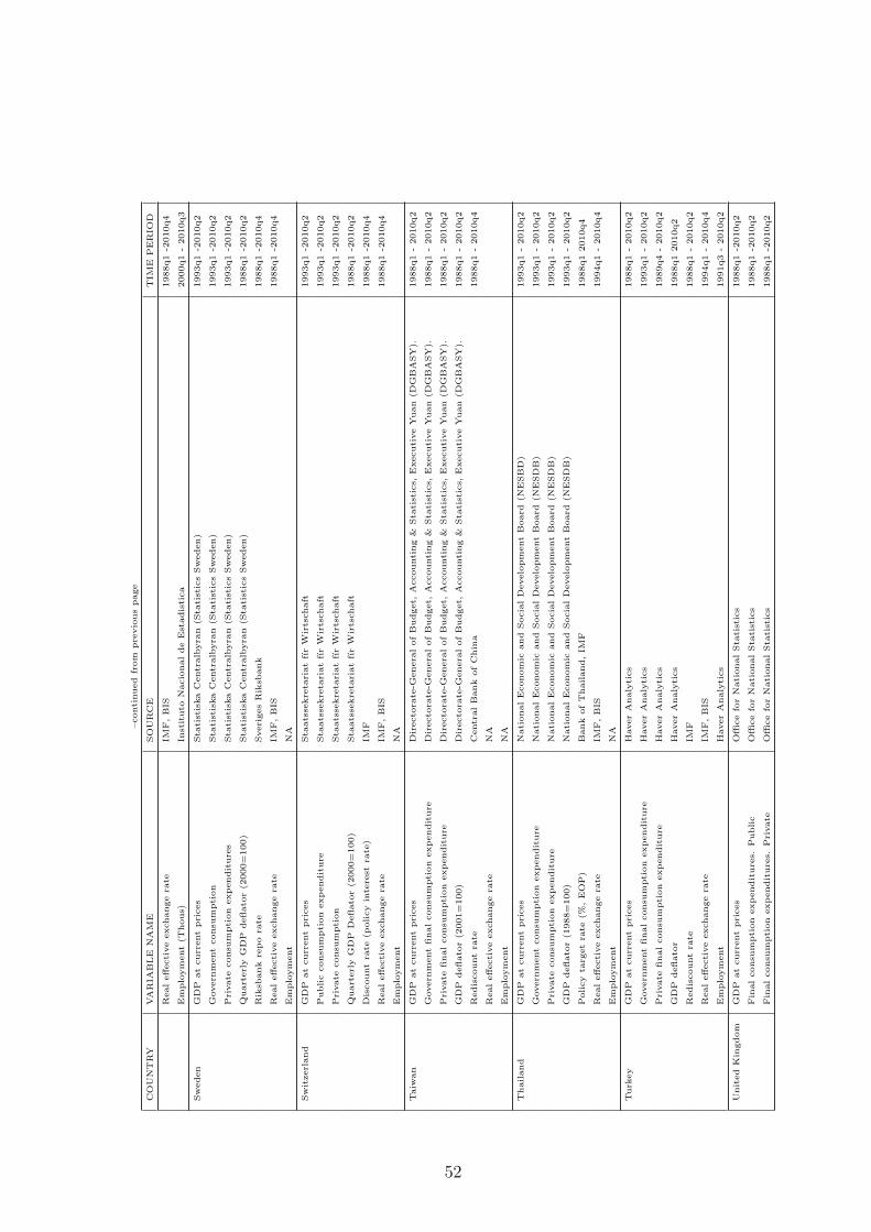
–conti

nued

from

pre

vio

us

page

CO

UN

TRY

VA

RIA

BLE

NA

ME

SO

UR

CE

TIM

EPER

IOD

Realeffecti

ve

exchange

rate

IMF,B

IS1988q1

-2010q4

Em

plo

ym

ent

(Thous)

Inst

ituto

Nacio

nalde

Est

adis

tica

2000q1

-2010q3

Sw

eden

GD

Pat

curr

ent

pri

ces

Sta

tist

iska

Centr

alb

yra

n(S

tati

stic

sSw

eden)

1993q1

-2010q2

Govern

ment

consu

mpti

on

Sta

tist

iska

Centr

alb

yra

n(S

tati

stic

sSw

eden)

1993q1

-2010q2

Pri

vate

consu

mpti

on

expendit

ure

sSta

tist

iska

Centr

alb

yra

n(S

tati

stic

sSw

eden)

1993q1

-2010q2

Quart

erl

yG

DP

deflato

r(2

000=

100)

Sta

tist

iska

Centr

alb

yra

n(S

tati

stic

sSw

eden)

1988q1

-2010q2

Rik

sbank

repo

rate

Sveri

ges

Rik

sbank

1988q1

-2010q4

Realeffecti

ve

exchange

rate

IMF,B

IS1988q1

-2010q4

Em

plo

ym

ent

NA

Sw

itzerl

and

GD

Pat

curr

ent

pri

ces

Sta

ats

sekre

tari

at

fır

Wir

tschaft

1993q1

-2010q2

Public

consu

mpti

on

expendit

ure

Sta

ats

sekre

tari

at

fır

Wir

tschaft

1993q1

-2010q2

Pri

vate

consu

mpti

on

Sta

ats

sekre

tari

at

fır

Wir

tschaft

1993q1

-2010q2

Quart

erl

yG

DP

Deflato

r(2

000=

100)

Sta

ats

sekre

tari

at

fır

Wir

tschaft

1988q1

-2010q2

Dis

count

rate

(policy

inte

rest

rate

)IM

F1988q1

-2010q4

Realeffecti

ve

exchange

rate

IMF,B

IS1988q1

-2010q4

Em

plo

ym

ent

NA

Taiw

an

GD

Pat

curr

ent

pri

ces

Dir

ecto

rate

-Genera

lofB

udget,

Accounti

ng

&Sta

tist

ics,

Executi

ve

Yuan

(DG

BA

SY

).1988q1

-2010q2

Govern

ment

finalconsu

mpti

on

expendit

ure

Dir

ecto

rate

-Genera

lofB

udget,

Accounti

ng

&Sta

tist

ics,

Executi

ve

Yuan

(DG

BA

SY

).1988q1

-2010q2

Pri

vate

finalconsu

mpti

on

expendit

ure

Dir

ecto

rate

-Genera

lofB

udget,

Accounti

ng

&Sta

tist

ics,

Executi

ve

Yuan

(DG

BA

SY

).1988q1

-2010q2

GD

Pdeflato

r(2

001=

100)

Dir

ecto

rate

-Genera

lofB

udget,

Accounti

ng

&Sta

tist

ics,

Executi

ve

Yuan

(DG

BA

SY

).1988q1

-2010q2

Redis

count

rate

Centr

alB

ank

ofC

hin

a1988q1

-2010q4

Realeffecti

ve

exchange

rate

NA

Em

plo

ym

ent

NA

Thailand

GD

Pat

curr

ent

pri

ces

Nati

onalEconom

icand

Socia

lD

evelo

pm

ent

Board

(NESB

D)

1993q1

-2010q2

Govern

ment

consu

mpti

on

expendit

ure

Nati

onalEconom

icand

Socia

lD

evelo

pm

ent

Board

(NESD

B)

1993q1

-2010q2

Pri

vate

consu

mpti

on

expendit

ure

Nati

onalEconom

icand

Socia

lD

evelo

pm

ent

Board

(NESD

B)

1993q1

-2010q2

GD

Pdeflato

r(1

988=

100)

Nati

onalEconom

icand

Socia

lD

evelo

pm

ent

Board

(NESD

B)

1993q1

-2010q2

Policy

targ

et

rate

(%,EO

P)

Bank

ofT

hailand,IM

F1988q1

2010q4

Realeffecti

ve

exchange

rate

IMF,B

IS1994q1

-2010q4

Em

plo

ym

ent

NA

Turk

ey

GD

Pat

curr

ent

pri

ces

Haver

Analy

tics

1988q1

-2010q2

Govern

ment

finalconsu

mpti

on

expendit

ure

Haver

Analy

tics

1993q1

-2010q2

Pri

vate

finalconsu

mpti

on

expendit

ure

Haver

Analy

tics

1989q4

-2010q2

GD

Pdeflato

rH

aver

Analy

tics

1988q1

2010q2

Redis

count

rate

IMF

1988q1

-2010q2

Realeffecti

ve

exchange

rate

IMF,B

IS1994q1

-2010q4

Em

plo

ym

ent

Haver

Analy

tics

1991q3

-2010q2

Unit

ed

Kin

gdom

GD

Pat

curr

ent

pri

ces

Offi

ce

for

Nati

onalSta

tist

ics

1988q1

-2010q2

Fin

alconsu

mpti

on

expendit

ure

s.Public

Offi

ce

for

Nati

onalSta

tist

ics

1988q1

-2010q2

Fin

alconsu

mpti

on

expendit

ure

s.Pri

vate

Offi

ce

for

Nati

onalSta

tist

ics

1988q1

-2010q2

52

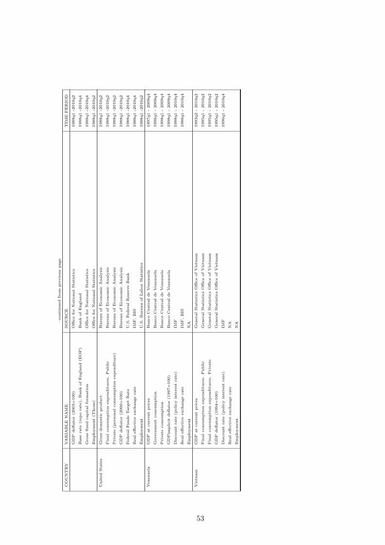
–conti

nued

from

pre

vio

us

page

CO

UN

TRY

VA

RIA

BLE

NA

ME

SO

UR

CE

TIM

EPER

IOD

GD

Pdeflato

r(2

003=

100)

Offi

ce

for

Nati

onalSta

tist

ics

1988q1

-2010q2

Base

rate

(repo

rate

),B

ank

ofEngla

nd

(EO

P)

Bank

ofEngla

nd

1988q1

-2010q4

Gro

ssfixed

capit

alfo

rmati

on

Offi

ce

for

Nati

onalSta

tist

ics

1988q1

-2010q4

Em

plo

ym

ent

(Thous)

Offi

ce

for

Nati

onalSta

tist

ics

1988q1

-2010q2

Unit

ed

Sta

tes

Gro

ssdom

est

icpro

duct

Bure

au

ofEconom

icA

naly

sis

1988q1

-2010q2

Fin

alconsu

mpti

on

expendit

ure

s.Public

Bure

au

ofEconom

icA

naly

sis

1988q1

-2010q2

Pri

vate

(pers

onalconsu

mpti

on

expendit

ure

)B

ure

au

ofEconom

icA

naly

sis

1988q1

-2010q2

GD

Pdeflato

r(2

000=

100)

Bure

au

ofEconom

icA

naly

sis

1988q1

-2010q2

Federa

lFunds

Targ

et

Rate

U.S

.Federa

lR

ese

rve

Bank

1988q1

-2010q4

Realeffecti

ve

exchange

rate

IMF,B

IS1988q1

-2010q4

Em

plo

ym

ent

U.S

.B

ure

au

ofLabor

Sta

tist

ics

1988q1

-2010q2

Venezuela

GD

Pat

curr

ent

pri

ces

Banco

Centr

alde

Venezuela

1997q1

-2009q4

Govern

ment

consu

mpti

on

Banco

Centr

alde

Venezuela

1998q1

-2009q4

Pri

vate

consu

mpti

on

Banco

Centr

alde

Venezuela

1998q1

-2009q4

GD

Pim

plicit

deflato

r(1

997=

100)

Banco

Centr

alde

Venezuela

1998q1

-2009q4

Dis

count

rate

(policy

inte

rest

rate

)IM

F1988q1

-2010q4

Realeffecti

ve

exchange

rate

IMF,B

IS1988q1

-2010q4

Em

plo

ym

ent

NA

Vie

tnam

GD

Pat

curr

ent

pri

ces

Genera

lSta

tist

ics

Offi

ce

ofV

ietn

am

1993q2

-2010q2

Fin

alconsu

mpti

on

expendit

ure

s.Public

Genera

lSta

tist

ics

Offi

ce

ofV

ietn

am

1995q1

-2010q2

Fin

alconsu

mpti

on

expendit

ure

s.Pri

vate

Genera

lSta

tist

ics

Offi

ce

ofV

ietn

am

1995q1

-2010q2

GD

Pdeflato

r(1

994=

100)

Genera

lSta

tist

ics

Offi

ce

ofV

ietn

am

1995q1

-2010q2

Dis

count

rate

(policy

inte

rest

rate

)IM

F1996q1

-2010q4

Realeffecti

ve

exchange

rate

NA

Em

plo

ym

ent

NA

53