Fiscal Federalism and the Leviathan: The Evil Beast or the Lesser Evil?

Christina Berberich, Kiel Institute for World Economics

Johannes M. Metzler, Kiel Institute for World Economics

Abstract

This paper analyses the relation between fiscal decentralization and the size of government in the tradition of the Leviathan Hypothesis. We construct and include more comprehensive indicators of fiscal federalism than the classical sub-national revenue and expenditure shares by using structural aspects of decentralization. The cross-sectional regression analysis for 21 high-income OECD countries shows that our indicators are of higher explanatory power and that, contrary to the Leviathan Hypothesis, a low degree of fiscal decentralization is related to lower public expenditures than a medium degree. The results underline the need to examine further in what ways federalism in countries with medium decentralization is misdesigned to cause higher public expenditures.

Key words: Fiscal federalism; Public expenditures; Leviathan hypothesis JEL Classification: H77, E62, C31 Corresponding author: Johannes M. Metzler, Kiel Institute for World Economics, Düsternbrooker Weg 120, 24105 Kiel, phone: +49 179 9222712, fax: +49 6221 474514, johannes.metzler@gmx.net. Co-author: Christina Berberich, Kiel Institute for World Economics, Düsternbrooker Weg 120, 24105 Kiel, phone: +49 179 779 2325, christina.berberich@web.de. Note: The authors wish to thank Dr. Jürgen Stehn for helpful comments and suggestions.

- 1 -

I. INTRODUCTION

Since the publication of the Leviathan Hypothesis by Brennan/Buchanan (1980) there has

been a considerable amount of research in the area of fiscal decentralization1 and its influence

on state performance variables, especially public expenditures. All empirical studies face the

same problem, which is to construct a measure of fiscal decentralization across countries

against which the hypothesis can be tested. Typical indicators of such studies are the share of

sub-national public expenditures as part of national public expenditure, as well as the revenue

generated on a sub-national level as a share of national revenue. Their simplicity is of

advantage, but obviously ‘fiscal reality’ can hardly be grasped in full by these two ratios.

In order to improve existing studies on the Leviathan Hypothesis, in our view it is useful to

create a more comprehensive indicator of fiscal federalism, generated out of qualitative

information of the structure and degree of fiscal relations within countries. This indicator

could provide a considerably better measure of fiscal decentralization and thus help to

improve the significance of empirical results. Also, such measure should not only be applied

to simply test for a linear relationship as it is usually done. A non-linear, polynomial

relationship between decentralization and public expenditures might also be a predictable

outcome of the theory of fiscal federalism.

The paper is organized as follows: Section II contains a brief introduction on the Leviathan

Hypothesis and the Theory of fiscal decentralization. Section III reviews existing empirical

findings on the effect of fiscal decentralization on public expenditures. Section IV lays out the

foundations of our empirical work in detail, i.e., the data used, the methodology of the

analysis and finally our results along with an interpretation and implications for future work.

Section V contains concluding remarks.

1 We use the terms federalism and decentralization synonymously in this paper. Also, when speaking of federalism and decentralization, the fiscal aspects involved are our main concern as opposed to the political or any other aspects.

- 2 -

II. THE LEVIATHAN HYPOTHESIS AND THE THEORY OF FISCAL FEDERALISM

The relation between fiscal decentralization and the size of government (or equivalently:

public expenditures) is based on the theory of the Leviathan State by Brennan and Buchanan

(1980). They assume that “total government intrusion into the economy should be smaller,

ceteris paribus, the greater the extent to which taxes and expenditures are decentralized”.2 The

theory states that tax competition is a constraint on the growth of government spending in

decentralized countries. The central government is seen as a hungry beast, a revenue-

maximizing monolithic entity, the Leviathan. This Leviathan can be tamed by destroying its

monopoly on taxation and bringing government spending closer to the preferences of the

people. The Theory of Fiscal Federalism implies that by shifting power from sub-national to

central government levels the preferences of individuals are neglected. Public spending by the

central government is always a compromise between the preferences of different regions and

citizens. The loss of welfare increases as the regional preferences diverge, the so-called

“Oates effect”3. Avoiding such a compromise is possible through fiscal decentralization under

the (rather strong) assumption of mobile individuals and firms which force local governments

to take part in tax competition.

The interest in fiscal decentralization has been increasing over the last decade. As Martinez-

Vazquez and McNab (2003) state, one reason is the belief that through fiscal decentralization

the efficiency of public expenditures can be enhanced. Another interpretation is that fiscal

decentralization can be a way to loosen the central government’s influence on the economy by

reallocating fiscal authority to sub-national government.

Thießen (2003) summarizes other positive characteristics of fiscal decentralization. Out of

these, one of the most important ones is the “diversification hypothesis” or Oates´

2 Brennan/Buchanan (1980), p. 15. 3 Stehn (2002), p. 302.

- 3 -

“decentralization theorem” which articulates that a central or uniform supply of public goods

and services will be generally inefficient. Considering these arguments, the size of

government should constantly decrease with increasing fiscal decentralization.

Nevertheless, there are arguments against full fiscal decentralization such as the view that it

intensifies regional inequalities. Also, lower quality of government decisions, more corruption

and greater influence of interest groups might be the outcome.4 With regard to the level of

public expenditures, decentralization might also lead to some increase due to foregone

economies of scale at the central level.5 Such reasoning extends the theory to a point where

one might expect an optimal influence of federalism on the size of government at some

medium degree of, and not absolute, decentralization.

III. BRIEF REVIEW OF EMPIRICAL LITERATURE ON FISCAL DECENTRALIZATION AND STATE PERFORMANCE

The Leviathan hypothesis has been subject of many empirical studies. But as Feld,

Kirchgässner and Schaltegger (2003) review, cross-national studies have largely failed to

prove the Leviathan Hypothesis. For Wallace Oates the Leviathan is a “mythical beast”6. As

an indicator of fiscal decentralization most authors used either the ratio of sub-national

expenditures to total expenditures or the ratio of sub-national revenue to total revenue.

Ehdaie (1994) extends all previous studies by using a cross-indicator (ratio of sub-national

governments own-source revenues over total national-sub-national government expenditures)

to treat the revenue and the spending side simultaneously, as he considers them indivisible.

His findings show a negative influence of decentralization on public sector size.

Rodden (2003) uses an error correction model with lagged variables to explain the growth of

government. His indicators for fiscal decentralization are the share of grants to total revenue

and the share of “own-source” sub-national revenue to total national revenue. His data set

4 Cp. Thießen (2003), p. 241. 5 Cp. OECD (2002b), p. 14. 6 Oates (1985), p. 756.

- 4 -

contains observations of 44 countries over the period 1978-97. The results also associate

decentralization with smaller government.

IV. METHODOLOGY, DATA AND EMPIRICAL ANALYSIS

IV.1. Classical and Revised Methodology

Traditionally, empirical studies on the Leviathan hypothesis follow a certain methodology.

There is a set of classical indicators of fiscal decentralization which are subsequently used to

test for a linear relationship between these indicators and the level of public expenditures

(measured as a share of GDP). Most often ratios of sub-national revenues as part of total

national revenues or sub-national expenditures as part of total national public expenditures are

used to capture the level of decentralization. Yet, it is often argued in the literature that these

indicators do not mirror the actual degree of sub-national responsibility over revenues and

expenditures, as the shares do not automatically correspond to autonomy and discretionary

power. Contrarily, often the central government decides on sub-national tax regulations (i.e.,

their tax bases and rates) and sets expenditure schemes and obligations.7 This implies that

such indicators cannot picture the reality of fiscal decentralization and its consequences

adequately.

In addition to the use of such indicators, a purely linear relation between decentralization and

the size of the government may not be the only possibility. The theory of fiscal federalism

predicts increasing constraints on the revenue-maximizing Leviathan with an increasing

degree of decentralization; yet its above-mentioned disadvantages may at some degree

dominate the advantages and actually result in an increase in public expenditures, e.g. due to

duplication of effort, corruption at the local level, etc.

This paper seeks to improve existing studies by using an advanced methodology. Firstly, a

wider range of decentralization indicators will be considered. Among the traditional above-

7 Cp. OECD (2003), p. 147.

- 5 -

mentioned indicators we aim to create additional, more comprehensive indicators: A more

detailed picture of fiscal decentralization can be drawn by help of a set of structural

decentralization indicators which are combined to form a more qualitative decentralization

ranking. We create these out of a recently published OECD survey on national budgetary

practices and procedures in 2002. By extending traditional decentralization indicators with

these additional data, it is possible to test if there are national structural factors which may

influence the amount of overall public expenditures. By transforming these indicators into

different indicators across our country sample, we can not only test for a linear relationship

but also for a non-linear, hump-shaped relationship.8 The logic behind such an estimation is to

incorporate the possibility of an optimal (or suboptimal) degree of fiscal decentralization

somewhere in the middle. Overall, this approach serves to provide a better understanding of

the issue at hand, namely the influence of fiscal decentralization on public expenditures.

IV.2. Estimation Method and Country Sample

The econometric estimation of this paper is based on a cross-country analysis of 21 high-

income OECD countries, as listed in table 1. Excluded from the sample is Luxembourg

because of its small size, as well as the middle-income OECD countries.9 In order to smooth

out very short-term fluctuations in the amount of public expenditures and the sub-national

revenue and expenditure shares, the estimation is carried out with data averages over the

period 1998-2000.10 Such a cross-country comparison implicitly assumes that long-term

equilibria in the respective variables have been reached. Looking at changes in the last three

decades such a conclusion may be premature. Yet, this assumption is more realistic for the

group of high-income OECD countries than for any other country group. Thus the group is

chosen for reasons of homogeneity, comparability, stability and data reliability. Also, Thießen

8 Such an approach was used by Thießen (2003) for high-income OECD countries with growth of GDP as the endogenous variable. 9 Czech Republic, Hungary, Iceland, Korea, Mexico, Poland, Slovak Republic and Turkey. 10 In some cases shorter periods or single-year figures apply due to data constraints.

- 6 -

(2003) concludes that most high-income OECD countries have converged to a medium degree

of fiscal federalism over the last three decades, which underlines the assumption that no major

changes may be expected in the near future.

IV.3. Indicators of Fiscal Decentralization

IV.3.a. Classical Indicators: Governmental System and Sub-national Expenditure/ Revenue Shares

The use of sub-national expenditure and revenue shares as explanatory variables for the level

of public expenditures is suggested by both the Theory of Fiscal Federalism and the Leviathan

Hypothesis. We applied three year averages over the years 1998-2000 in order to smoothen

out short-term variations in the shares.11 These indicators (exp_share and rev_share) are listed

in table 1 for our country sample of 21 high-income OECD countries.

Table 1: Classical Indicators of Fiscal Decentralisation

gov_sys rev_share exp_share avg_share

Governmental

System Sub-national

Revenue Share Sub-national

Expenditure Share Avg. of rev_share

and exp_share

AUSTRALIA federal 32.0 42.5 37.3 AUSTRIA federal 24.9 31.6 28.2 BELGIUM federal 10.1 24.1 17.1 CANADA federal 52.2 58.7 55.4 DENMARK unitary 33.4 46.1 39.7 FINLAND unitary 27.7 33.5 30.6 FRANCE unitary 12.5 16.3 14.4 GERMANY federal 32.7 38.5 35.6 GREECE unitary 3.4 3.9 3.6 IRELAND unitary 6.9 25.1 16.0 ITALY unitary 16.7 24.1 20.4 JAPAN unitary 26.0 40.7 33.4 NETHERLANDS unitary 10.9 27.7 19.3 NEW ZEALAND unitary 10.8 10.7 10.7 NORWAY unitary 21.1 34.0 27.5 PORTUGAL unitary 8.4 10.4 9.4 SPAIN unitary 18.9 27.6 23.3 SWEDEN unitary 31.8 36.9 34.4 SWITZERLAND federal 42.9 47.4 45.2 UNITED KINGDOM unitary 8.1 22.1 15.1 UNITED STATES federal 41.4 49.5 45.5

Note: Three-year averages 1998-2000 where no data restrictions apply. Exceptions: France (2000), Germany (1998 and 2000), Ireland (1997), Japan (2000), Netherlands (2000), Norway (1998 and 1999). Source: IMF Government Finance Statistics Yearbook (GFSY) 2002 and 2003; Japan: OECD Economic Outlook 2003; authors’ calculations. 11 For some countries, only one or two year data is applied due to data constraints.

- 7 -

Additionally, a dummy variable was created indicating if a country’s governmental system is

formally federal or unitary.12 Interestingly, this classification seems to be in no obvious

relation to the degree of decentralization as measured in any of the other indicators, an

observation that was made before (cp. Thießen (2003), p. 259, OECD (2003), p. 144) and was

confirmed through persistent insignificance of this dummy variable in the forthcoming

estimation.

IV.3b. Structural Indicators: Expenditure and Revenue Decentralization Index

The structural decentralization indicators were formed out of the OECD/World Bank Budget

Practices and Procedures Database, providing comparable data on nearly 300 aspects of the

budget formulation, approval, implementation and audit phases in each OECD member

country except Switzerland and many non-member countries. Aspects of fiscal interrelations

between government levels are contained in section 6 of the database. Out of this section, we

chose the most important aspects which indicate higher or lower degrees of decentralization

with regard to revenue and expenditure autonomy. For every of the chosen aspects a dummy

variable was created where 1 indicates a high degree of decentralization or sub-national

autonomy and 0 a low degree of decentralization with respect to the survey question.13 In a

limited number of cases 0.5 was given in case of answers which were ambiguous or not given.

In order to facilitate reference to the original survey questions for the reader, the components

of our decentralization ranking contain the number of the original survey question.

12 Cp. Thießen (2003), p. 245. 13 For Switzerland no survey data was existing, so the data was investigated with help of additional literature, as well as for the completion of data sets for some other countries where survey data was missing.

- 8 -

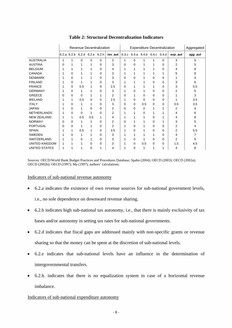
Table 2: Structural Decentralization Indicators

Revenue Dezentralization Expenditure Decentralization Aggregated 6.2.a 6.2.b 6.2.d 6.2.e 6.2.h rev_aut 6.3.c 6.4.a 6.4.b 6.4.c 6.4.d exp_aut agg_aut

AUSTRALIA 1 1 0 0 0 2 1 0 1 1 0 3 5 AUSTRIA 0 1 1 1 0 3 0 0 1 1 0 2 5 BELGIUM 1 1 1 1 0 4 1 1 1 1 0 4 8 CANADA 1 0 1 1 0 3 1 1 1 1 1 5 8 DENMARK 1 0 1 1 0 3 0 0 1 0 0 1 4 FINLAND 1 0 1 1 0 3 1 1 1 0 0 3 6 FRANCE 1 0 0.5 1 0 2.5 0 1 1 1 0 3 5.5 GERMANY 1 0 1 1 0 3 1 0 1 0 0 2 5 GREECE 0 0 0 1 1 2 0 1 0 0 0 1 3 IRELAND 1 1 0.5 0 0 2.5 1 0 0 0 0 1 3.5 ITALY 1 0 1 1 0 3 0 0 0.5 0 0 0.5 3.5 JAPAN 1 0 1 0 0 2 0 0 0 1 1 2 4 NETHERLANDS 1 0 0 1 0 2 1 1 0 1 1 4 6 NEW ZEALAND 1 1 0.5 0.5 1 4 1 1 1 0 1 4 8 NORWAY 0 0 1 1 0 2 0 1 1 0 1 3 5 PORTUGAL 0 0 1 1 0 2 1 0 1 0 0 2 4 SPAIN 1 1 0.5 1 0 3.5 1 0 1 0 0 2 5.5 SWEDEN 1 0 1 1 0 3 1 1 1 1 0 4 7 SWITZERLAND 1 1 0 1 0 3 1 0 1 0 0 2 5 UNITED KINGDOM 1 1 1 0 0 3 1 0 0.5 0 0 1.5 4.5 UNITED STATES 1 1 1 0 1 4 1 0 1 1 1 4 8

Sources: OECD/World Bank Budget Practices and Procedures Database; Spahn (2004); OECD (2003); OECD (2002a); OECD (2002b); OECD (1997); Ma (1997); authors’ calculations.

Indicators of sub-national revenue autonomy

• 6.2.a indicates the existence of own revenue sources for sub-national government levels,

i.e., no sole dependence on downward revenue sharing.

• 6.2.b indicates high sub-national tax autonomy, i.e., that there is mainly exclusivity of tax

bases and/or autonomy in setting tax rates for sub-national governments.

• 6.2.d indicates that fiscal gaps are addressed mainly with non-specific grants or revenue

sharing so that the money can be spent at the discretion of sub-national levels.

• 6.2.e indicates that sub-national levels have an influence in the determination of

intergovernmental transfers.

• 6.2.h. indicates that there is no equalization system in case of a horizontal revenue

imbalance.

Indicators of sub-national expenditure autonomy

- 9 -

• 6.3.a indicates the existence of clear and separate competences for national and sub-

national governments for most of the expenditure.

• 6.4.a indicates the absence of borrowing limits for lower levels of government.

• 6.4.b indicates that the national government does not explicitly or implicitly guarantee the

borrowing activity of lower levels of government.

• 6.4.c indicates that the national government is not involved in setting the overall

expenditure level of lower layers of government.

• 6.4.d indicates that national government does not co-ordinate general government

expenditure aggregates.

Out of these dummy variables the following structural indicators were created: sub-national

revenue autonomy (rev_aut), sub-national expenditure autonomy (exp_aut) and aggregated

sub-national fiscal autonomy (agg_aut)14.

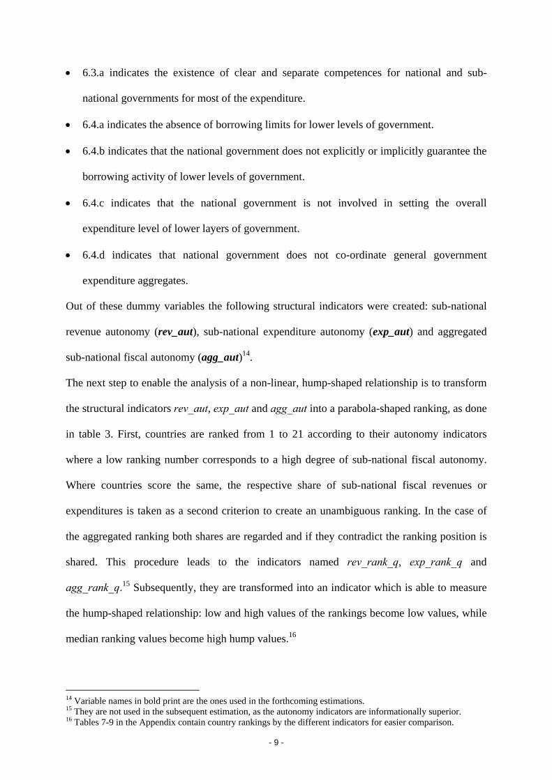
The next step to enable the analysis of a non-linear, hump-shaped relationship is to transform

the structural indicators rev_aut, exp_aut and agg_aut into a parabola-shaped ranking, as done

in table 3. First, countries are ranked from 1 to 21 according to their autonomy indicators

where a low ranking number corresponds to a high degree of sub-national fiscal autonomy.

Where countries score the same, the respective share of sub-national fiscal revenues or

expenditures is taken as a second criterion to create an unambiguous ranking. In the case of

the aggregated ranking both shares are regarded and if they contradict the ranking position is

shared. This procedure leads to the indicators named rev_rank_q, exp_rank_q and

agg_rank_q.15 Subsequently, they are transformed into an indicator which is able to measure

the hump-shaped relationship: low and high values of the rankings become low values, while

median ranking values become high hump values.16

14 Variable names in bold print are the ones used in the forthcoming estimations. 15 They are not used in the subsequent estimation, as the autonomy indicators are informationally superior. 16 Tables 7-9 in the Appendix contain country rankings by the different indicators for easier comparison.

- 10 -

Table 3: Structural Decentralization Indicators, Ranks and Humps

Revenue Autonomy Expenditure Autonomy Aggregated Autonomy

rev_aut

rev_ share

rev_ rank_q

rev_ hump_q

exp_aut

exp_share

exp_ rank_q

exp_ hump_q

agg_ aut

agg_ rank_q

agg_ hump_q

AUSTRALIA 2 32.0 16 6 3 42.5 7 7 5 11 11 AUSTRIA 3 24.9 11 11 2 31.6 14 8 5 12 10 BELGIUM 4 10.1 3 3 4 24.1 5 5 8 4.5 4.5 CANADA 3 52.2 5 5 5 58.7 1 1 8 2 2 DENMARK 3 33.4 7 7 1 46.1 18 4 4 14 8 FINLAND 3 27.7 10 10 3 33.5 9 9 6 8 8 FRANCE 2.5 12.5 14 8 3 16.3 10 10 5.5 13 9 GERMANY 3 32.7 8 8 2 38.5 13 9 5 9 9 GREECE 2 3.4 21 1 1 3.9 20 2 3 21 1 IRELAND 2.5 6.9 15 7 1 25.1 19 3 3.5 18.5 3.5 ITALY 3 16.7 12 10 0.5 24.1 21 1 3.5 17 5 JAPAN 2 26.0 17 5 2 40.7 12 10 4 20 2 NETHERLANDS 2 10.9 19 3 4 27.7 4 4 6 10 10 NEW ZEALAND 4 10.8 2 2 4 10.7 6 6 8 4.5 4.5 NORWAY 2 21.1 18 4 3 34.0 8 8 5 15 7 PORTUGAL 2 8.4 20 2 2 10.4 16 6 4 18.5 3.5 SPAIN 3.5 18.9 4 4 2 27.6 15 7 5.5 7 7 SWEDEN 3 31.8 9 9 4 36.9 3 3 7 3 3 SWITZERLAND 3 42.9 6 6 2 47.4 11 11 5 6 6 UNITED KINGDOM 3 8.1 13 9 1.5 22.1 17 5 4.5 16 6 UNITED STATES 4 41.4 1 1 4 49.5 2 2 8 1 1

Source: authors’ calculations.

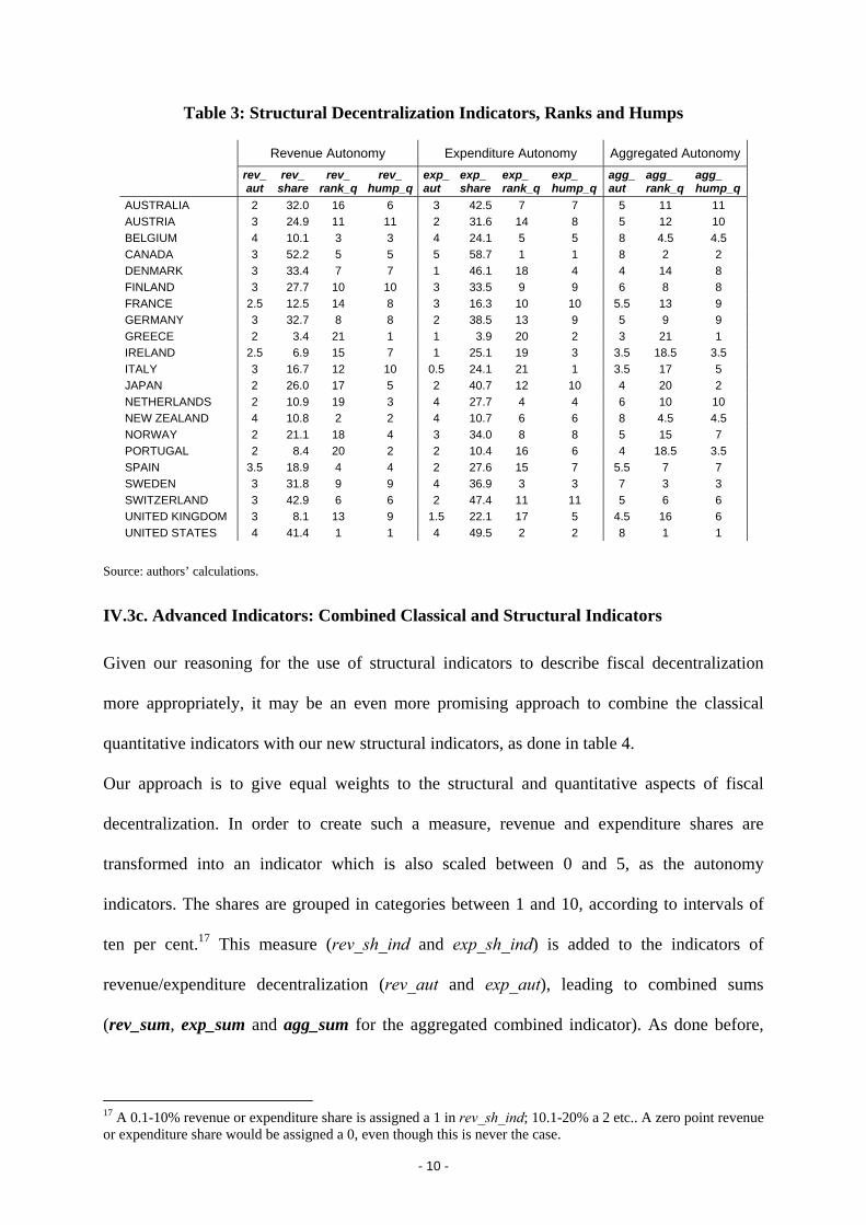
IV.3c. Advanced Indicators: Combined Classical and Structural Indicators

Given our reasoning for the use of structural indicators to describe fiscal decentralization

more appropriately, it may be an even more promising approach to combine the classical

quantitative indicators with our new structural indicators, as done in table 4.

Our approach is to give equal weights to the structural and quantitative aspects of fiscal

decentralization. In order to create such a measure, revenue and expenditure shares are

transformed into an indicator which is also scaled between 0 and 5, as the autonomy

indicators. The shares are grouped in categories between 1 and 10, according to intervals of

ten per cent.17 This measure (rev_sh_ind and exp_sh_ind) is added to the indicators of

revenue/expenditure decentralization (rev_aut and exp_aut), leading to combined sums

(rev_sum, exp_sum and agg_sum for the aggregated combined indicator). As done before,

17 A 0.1-10% revenue or expenditure share is assigned a 1 in rev_sh_ind; 10.1-20% a 2 etc.. A zero point revenue or expenditure share would be assigned a 0, even though this is never the case.

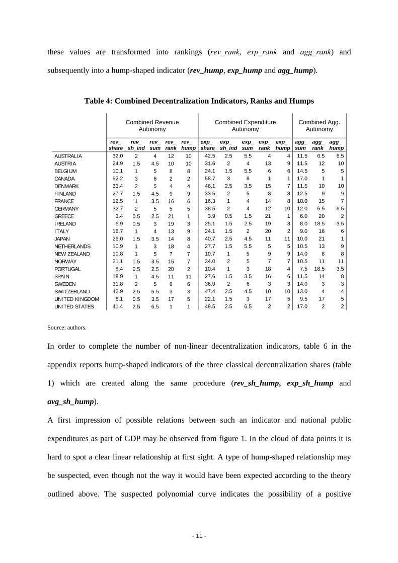
- 11 -

these values are transformed into rankings (rev_rank, exp_rank and agg_rank) and

subsequently into a hump-shaped indicator (rev_hump, exp_hump and agg_hump).

Table 4: Combined Decentralization Indicators, Ranks and Humps

Combined Revenue Autonomy

Combined Expenditure Autonomy

Combined Agg. Autonomy

rev_share

rev_ sh_ind

rev_ sum

rev_rank

rev_hump

exp_share

exp_ sh_ind

exp_sum

exp_rank

exp_ hump

agg_ sum

agg_ rank

agg_hump

AUSTRALIA 32.0 2 4 12 10 42.5 2.5 5.5 4 4 11.5 6.5 6.5AUSTRIA 24.9 1.5 4.5 10 10 31.6 2 4 13 9 11.5 12 10BELGIUM 10.1 1 5 8 8 24.1 1.5 5.5 6 6 14.5 5 5CANADA 52.2 3 6 2 2 58.7 3 8 1 1 17.0 1 1DENMARK 33.4 2 5 4 4 46.1 2.5 3.5 15 7 11.5 10 10FINLAND 27.7 1.5 4.5 9 9 33.5 2 5 8 8 12.5 9 9FRANCE 12.5 1 3.5 16 6 16.3 1 4 14 8 10.0 15 7GERMANY 32.7 2 5 5 5 38.5 2 4 12 10 12.0 6.5 6.5GREECE 3.4 0.5 2.5 21 1 3.9 0.5 1.5 21 1 6.0 20 2IRELAND 6.9 0.5 3 19 3 25.1 1.5 2.5 19 3 8.0 18.5 3.5ITALY 16.7 1 4 13 9 24.1 1.5 2 20 2 9.0 16 6JAPAN 26.0 1.5 3.5 14 8 40.7 2.5 4.5 11 11 10.0 21 1NETHERLANDS 10.9 1 3 18 4 27.7 1.5 5.5 5 5 10.5 13 9NEW ZEALAND 10.8 1 5 7 7 10.7 1 5 9 9 14.0 8 8NORWAY 21.1 1.5 3.5 15 7 34.0 2 5 7 7 10.5 11 11PORTUGAL 8.4 0.5 2.5 20 2 10.4 1 3 18 4 7.5 18.5 3.5SPAIN 18.9 1 4.5 11 11 27.6 1.5 3.5 16 6 11.5 14 8SWEDEN 31.8 2 5 6 6 36.9 2 6 3 3 14.0 3 3SWITZERLAND 42.9 2.5 5.5 3 3 47.4 2.5 4.5 10 10 13.0 4 4UNITED KINGDOM 8.1 0.5 3.5 17 5 22.1 1.5 3 17 5 9.5 17 5UNITED STATES 41.4 2.5 6.5 1 1 49.5 2.5 6.5 2 2 17.0 2 2

Source: authors.

In order to complete the number of non-linear decentralization indicators, table 6 in the

appendix reports hump-shaped indicators of the three classical decentralization shares (table

1) which are created along the same procedure (rev_sh_hump, exp_sh_hump and

avg_sh_hump).

A first impression of possible relations between such an indicator and national public

expenditures as part of GDP may be observed from figure 1. In the cloud of data points it is

hard to spot a clear linear relationship at first sight. A type of hump-shaped relationship may

be suspected, even though not the way it would have been expected according to the theory

outlined above. The suspected polynomial curve indicates the possibility of a positive

- 12 -

relationship between the level of public expenditures and a medium level of

decentralization.18

Also, it can be clearly seen that there are some outlier countries which in no case follow a

common trend, most notably Japan and New Zealand.

Graph 1: Public Expenditure/GDP and Fiscal Decentralization in 21 High-Income OECD Countries

0.20

0.25

0.30

0.35

0.40

0.45

0.50

0.55

0.60

0.65

0.70

4.0 8.0 12.0 16.0 20.0

Fiscal Decentralization (agg_sum)

Publ

ic E

xpen

ditu

res

/ GD

P

Linear

Polynomial

Germany

Japan

New Zealand

Canada

USA

Belgium

Sweden

Denmark

Netherlands

France

Greece

PortugalIreland

Italy

UK

Australia

Spain

Austria

Finland

Switzerland

Norway

Note: Public expenditures and GDP are measured as three-year averages over the period 1998-2000. Source: GFSY 2002/2003, IMF International Financial Statistics (IFS) CD-ROM 2004.

IV.4. Variables and Estimation of Results

The dependent variable as suggested by the greater part of the Leviathan literature is the size

of government measured by the level of general government (i.e., including all levels of

government) public expenditures as a share of GDP (exp_gdp). The data were extracted from

18 Actually, there is a difference between a generally medium degree of decentralization and a medium degree of decentralization with regard to the respective country sample. However, it is clear that the total extremes do not exist, i.e., full centralization or full decentralization. In that sense we assume our sample to be one in which the range of actually feasible degrees of decentralization is covered at the extremes so that here both expressions express the same.

- 13 -

the IMF Government Financial Statistics and represent three-year averages over the years

1998-2000.19

A whole range of estimations will be carried out with the above introduced indicators of fiscal

decentralization, our independent variables. By doing so we pursue several goals: First, we

aim to find out which indicators provide us with best results: the classical quantitative

decentralization measures, structural decentralization measures or, as we suspect, combined

indicators. Second, we aim to explain if public expenditures can best be explained by

considering either the revenue aspects or the expenditure aspects of fiscal federalism, or if an

aggregation of both sides is needed to offer a meaningful explanation. These findings may

also provide a more profound clarification of the reasons for higher or lower public

expenditures, which may be rooted in very few main aspects of fiscal federalism design. Our

hypothesis is that either the expenditure side or the aggregated indicators should perform best

to explain public expenditures. Third, we aim to verify whether the size of government

follows a linear or a non-linear trend. The Leviathan hypothesis predicts a (strictly) linear and

negative relation between the degree of fiscal decentralization and the level of public

expenditures. The theory of fiscal federalism combined with the explanations above predicts a

non-linear relation where public expenditures should be lowest at a medium degree of fiscal

decentralization.

To test these hypotheses, the size of the public sector is regressed on one of the indicators of

fiscal decentralization and a matrix of control variables suggested by the literature on public

sector size or growth. For the basic estimation procedure we use a limited set of control

variables in order to be left with sufficient degrees of freedom and to produce meaningful

results. Subsequently, the results can be tested for robustness by including more control

variables.20

19 Due to data constraints: France (2000), Germany (1998 and 2000), Ireland (1997), Japan (1993), Netherlands (2000), Norway (1998 and 1999). 20 The set of control variables was mainly adapted to our problem from the set of Rodden (2003).

- 14 -

Our basic matrix of control variables with a three-year average (1998-2000) includes: i) GDP

per capita21 (gdp_pc) in current US dollars where data are calculated from the World Bank

Development Indicators; ii) Trade openness (open) as measured by exports plus imports as a

share of GDP in current prices where data are from Penn World Tables for the years 1998-

2000; iii) A dummy for the national executive being controlled by the left taken from the

World Bank’s Database of Political Institutions (DPI) for the year 2000 (ex_left); iv) Fixed

country dummies22 (jpnwz23).

The extended set of control variables additionally contains: v) the size of the population

(popu) as taken from IFS; vi) the national dependency ratio24 (dep) as reported by World

Bank Development Indicators; vii) a dummy variable for parliamentary regimes (ex_parl, as

opposed to a directly elected executive power) also taken from DPI.

The basic regression (1) and the robust regression (2) look as follows, where log variables are

taken whenever possible to improve the fit of the estimation:

(1) ln exp_gdpi = α + β1 ln gdp_pci + β2 ln openi + β3 ex_lefti + β4 jpnwz

+ β5 ln decentralization indicatori

(2) ln exp_gdpi = α + β1 ln gdp_pci + β2 ln openi + β3 ex_lefti + β4 ln popui + β5 ln depi

+ β6 ex_parli + β7 jpnwz + β8 ln decentralization indicatori

Table 5 contains the estimation results of the basic estimation. Table 10 in the appendix

contains the robust estimations with the extended set of control variables.

21 According to Wagner’s Law. 22 Country dummies control for the existence of omitted variables in terms of fixed country effects which may help determine country differences in the long-term. The obvious fixed country dummy for different governmental systems gov_sys was universally estimated insignificant and is thus not reported. 23 Best results are achieved by controlling for the extreme outlier countries of Japan and New Zealand, which show abnormally low public expenditures. This may be explained by low levels of social security and social service expenditures in both countries. (Ministry of Finance Japan (2001), Atkinson and Noord (2001)) 24 The share of society above or below working age.

- 15 -

Table 5: Results of Basic Estimation

Dependent Variable: log General Government Public Expenditures / GDP [ln exp_gdp], 1998-2000

Eq. Decentralization measure α ln gdp_pc ln open ex_left jpnwz dec.

indicator Adj. R2 Akaike F-stat.

Rev. Autonomy

a1 ln rev_share 1.300 0.068 0.207 0.102 -0.439 0.030 0.713 -1.079 10.935 (2.385) (0.104) (0.063)*** (0.057)* (0.104)*** (0.051)

a2 ln rev_aut 0.668 0.098 0.191 0.098 -0.454 0.060 0.711 -1.074 10.860 (2.049) (0.084) (0.061)*** (0.057) (0.103)*** (0.119)

a3 ln rev_sum 1.108 0.077 0.197 0.098 -0.450 0.078 0.715 -1.087 11.038 (2.177) (0.092) (0.060)*** (0.057) (0.102)*** (0.116)

a4 ln rev_sh_hump 1.120 0.074 0.202 0.120 -0.483 0.080 0.779 -1.340 15.081 (1.804) (0.074) (0.053)*** (0.051)** (0.091)*** (0.036)**

a5 ln rev_hump_q 1.620 0.059 0.182 0.109 -0.436 0.052 0.732 -1.147 11.915 (2.154) (0.089) (0.060)*** (0.055)* (0.100)*** (0.044)

a6 ln rev_hump 1.045 0.082 0.172 0.145 -0.507 0.088 0.782 -1.357 15.388 (1.784) (0.073) (0.054)*** (0.053)** (0.093)*** (0.039)**

Exp. Autonomy

a7 ln exp_share -0.672 0.163 0.193 0.095 -0.462 -0.043 0.713 -1.081 10.954 (2.906) (0.129) (0.061)*** (0.058) (0.105)*** (0.072)

a8 ln exp_aut 0.250 0.117 0.202 0.114 -0.434 -0.033 0.714 -1.084 10.998 (2.093) (0.086) (0.061)*** (0.060)* (0.105)*** (0.051)

a9 ln exp_sum 0.037 0.128 0.200 0.108 -0.438 -0.040 0.711 -1.072 10.831 (2.335) (0.098) (0.061)*** (0.059)* (0.105)*** (0.083)

a10 ln exp_sh_hump 1.366 0.071 0.175 0.119 -0.457 0.044 0.723 -1.114 11.431 (2.170) (0.089) (0.063)** (0.059)* (0.101)*** (0.047)

a11 ln exp_hump_q 0.788 0.093 0.194 0.108 -0.464 0.026 0.714 -1.083 10.989 (2.059) (0.085) (0.060)*** (0.058)* (0.105)*** (0.042)

a12 ln exp_hump 1.898 0.047 0.175 0.115 -0.523 0.072 0.751 -1.220 13.044

(2.063) (0.085) (0.058)*** (0.054)** (0.106)*** (0.044)

Agg. Autonomy

a13 ln avg_share 0.330 0.116 0.195 0.101 -0.451 -0.009 0.707 -1.058 10.643 (2.729) (0.120) (0.062)*** (0.058) (0.105)*** (0.066)

a14 ln agg_aut 0.547 0.105 0.197 0.103 -0.447 -0.006 0.707 -1.057 10.630 (2.109) (0.088) (0.063)*** (0.060) (0.106)*** (0.106)

a15 ln agg_sum 0.727 0.095 0.195 0.100 -0.451 0.023 0.707 -1.059 10.656 (2.219) (0.096) (0.061)*** (0.058) (0.104)*** (0.126)

a16 ln avg_sh_hump 1.553 0.061 0.178 0.133 -0.462 0.060 0.737 -1.168 12.234 (2.081) (0.086) (0.059)*** (0.059)** (0.098)*** (0.045)

a17 ln agg_hump_q 1.299 0.074 0.156 0.121 -0.432 0.087 0.783 -1.359 15.425 (1.798) (0.074) (0.055)** (0.050)** (0.089)*** (0.038)**

a18 ln agg_hump 0.791 0.096 0.150 0.107 -0.424 0.099 0.811 -1.495 18.127 (1.655) (0.068) (0.052)** (0.046)** (0.084)*** (0.034)**

Source: authors’ calculations Note: Standard errors in brackets. ***p < .01, **p < .05, *p < .1.

- 16 -

IV.5. Interpretation of Results

Table 5 provides us with first answers to the questions posed above. Overall, all regressions

are of good explanatory power, with adjusted R2’s between 70 and 82 per cent.25 While the

constant α and gdp_pc are never significant, the other control variables perform well, with

openness open being always significant at the 5 or 10 per cent level, ex_left being mostly

significant at the 5 or 10 per cent level and the country dummy for Japan and New Zealand

jpnwz being universally significant at the 1 per cent level. According to the parameter values

higher GDP per capita, a governing left-wing party and more trade openness have a positive

influence on the level of public expenditures.

The performance of the decentralization indicators is very varying but it can instantly be

noticed that only non-linear indicators are statistically significant.26 Surprisingly, the

observation of graph 1 is confirmed through the positive parameter value of all hump

indicators: according to the way this indicator was constructed a medium degree of

decentralization goes along with a higher value and thus a stronger influence on public

expenditures. We estimate this relationship to be positive. Additionally, public expenditures at

the “centralized end” of the country spectrum are on average lower than on the “decentralized

end”.27 These findings cannot be supported by any of the above stated theories.

The next observation which can be made is that two out of three non-linear indicators become

significant at the 5 per cent level for the aggregated autonomy as well as the revenue

autonomy consideration, however not for the expenditure autonomy consideration. In total,

aggregated indicators are more significant than revenue indicators only. But as the aggregated 25 For all estimations the hypothesis of homoscedasticity cannot be rejected at a one per cent significance level (White Test). 26 Without the fixed country dummy, the adjusted R2 falls below 40 per cent in the least explanatory equations and hardly overcomes the 50 per cent mark in the best cases. When excluding the country dummy for Japan and New Zealand, the decentralization indicator in equation a18 remains significant at 5%. In a17 it is barely above 10%, whereas it becomes highly insignificant in a4 and a6. Such distortion in the results confirms the necessity for such a dummy variable, especially in such a small country sample. 27 Using agg_sum to rank the country sample it can be divided into three equally strong groups. Without Japan and New Zealand, the six most centralized countries have average public expenditures / GDP of 49.4 per cent while the most decentralized countries average around 52.4 per cent. With medium decentralization the average is 54.6 per cent.

- 17 -

indicators are per definition half driven by the outcome of the revenue indicators, the reasons

for excessive public expenditures may rather be found in the design of a nation’s revenue

decentralization than its expenditure decentralization. Again, this finding contradicts our

hypothesis and lacks an obvious explanation.

Regarding our last question another interesting result is achieved: in every category the non-

linear indicator which is constructed by combining both the structural aspects as well as the

quantitative aspects outperforms all other indicators. The most successful out of these

measures is the one regarding aggregated autonomy (agg_hump) which is highly significant

(almost at the 1 per cent level). When looking at all three categories it is not obvious if the

quantitative or the purely structural indicator has more explanatory power. However, it

becomes clear that there is a significant added value when combining quantitative and

structural aspects of fiscal decentralization. This finding is consistent with the expectations of

the authors and the motivation of this paper.

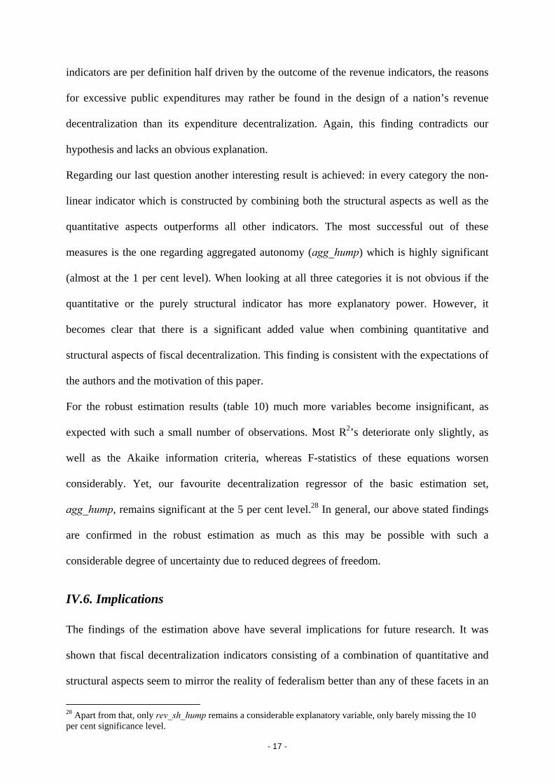
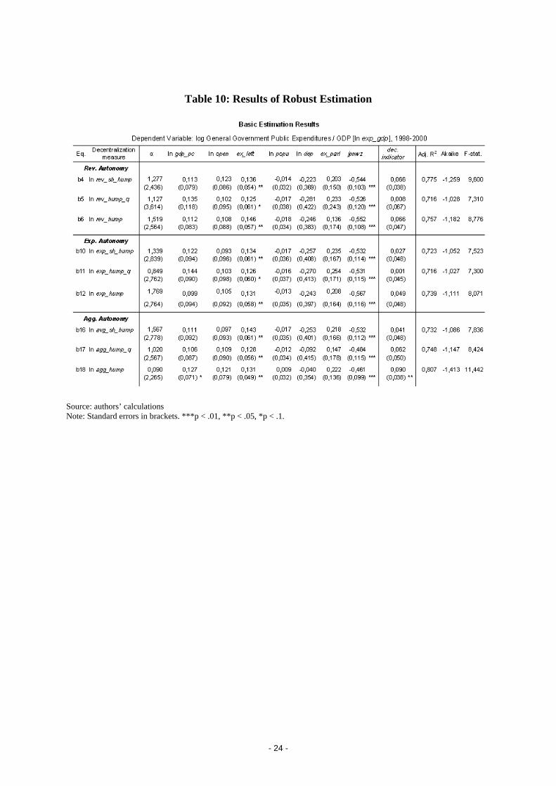
For the robust estimation results (table 10) much more variables become insignificant, as

expected with such a small number of observations. Most R2’s deteriorate only slightly, as

well as the Akaike information criteria, whereas F-statistics of these equations worsen

considerably. Yet, our favourite decentralization regressor of the basic estimation set,

agg_hump, remains significant at the 5 per cent level.28 In general, our above stated findings

are confirmed in the robust estimation as much as this may be possible with such a

considerable degree of uncertainty due to reduced degrees of freedom.

IV.6. Implications

The findings of the estimation above have several implications for future research. It was

shown that fiscal decentralization indicators consisting of a combination of quantitative and

structural aspects seem to mirror the reality of federalism better than any of these facets in an

28 Apart from that, only rev_sh_hump remains a considerable explanatory variable, only barely missing the 10 per cent significance level.

- 18 -

isolated consideration. Clearly such combined indicators may be challengeable as to their

composition. Different weighing of the composing survey aspects or the composing indicators

could lead to different results. Indicator fine-tuning might still be possible and should go

along with detailed investigation of the reasons for the surprising results of this study.29

This leads to the second finding and unanswered question – why do characteristics of revenue

decentralization explain public expenditure patterns more accurately than features of

expenditure decentralization? The answer may be found with help of the OECD/World Bank

Budget Practices and Procedures Database which is much more comprehensive than the data

used in this study. Apart from fiscal relations between different levels of government, more

detailed information is contained on various issues of national budgeting which may also be

of high influence on the level of public expenditures. In our view this data might also be used

to construct one overall or several sub-indicators on budgeting practices which would then

shed more light onto possible influences on the size of government.

In a practical sense, this approach may also yield answers to the second puzzle brought up in

this paper, the relation between comparatively higher public expenditures and a medium

degree of decentralization. For example, it seems plausible that an administration which is

decentralized “half-way” neither profits from economies of scale at the central level nor from

the improved matching of the preferences of local citizens. Instead, shared competences may

result in increased decision and coordination costs with bureaucratic efforts and state

employment at the national and sub-national level without the expenditure-minimizing

consequences of decentralization. Such thoughts may have far-reaching consequences for the

Theory of Fiscal Federalism which is likely to use overly simplistic assumptions and thus

29 For example, the actual amount of taxes over which sub-national governments have full discretion might be included as an indicator of federalism (Cp. Meloche, Vaillancourt and Yilmaz (2004)). This aspect was only coded as “mainly” or “not mainly” in our indicator. Also, the budgeting survey seems not to be filled out diligently at times. For example, Germany’s answer to 6.4.b indicates no bailing out of lower levels of government while the Federal Constitutional Court has made it clear that bankrupt sub-national governments cannot default but have to be supported vertically or horizontally. In general, a big obstacle for fine tuning is the lack of data availability and reliability which would have to be satisfied through extensive case studies of every country involved in the sample.

- 19 -

need to be extended. It seems reasonable to expect answers with regard to the institutional set-

up of fiscal federalism in practice and/or political incentives, i.e., in the domains of the NIE

(new institutional economics) or the NPE (new political economy). For example, it may be

interesting to examine if existing structures of fiscal federalism are designed along the lines of

Weingast’s (1995) “market-preserving federalism” and if deviations from this structure may

be responsible for excessive public expenditures. For example, while our indicator regards the

absence of borrowing limits for lower level governments as higher expenditure autonomy,

Weingast argues that soft budget constraints are one of the characteristics of federalism which

destroy market signals and thus lead to increased inefficiency.

It is an essential question to ask if the implementation of theoretically superior federalism

structures is inherently flawed or if they can be improved and thus lead to actually

quantifiable superiority, such as lower public expenditures. Before such additional analysis is

not carried out, it is probably too early to come up with detailed policy advice on how to

improve those structures.30

Also it should be taken in mind that the level of public expenditures is only one among

several key policy goals. Economic growth might be regarded an equally important goal

fostered through adequate fiscal structures. In that sense, our results differ from Thießen

(2003) who examines the impact of fiscal federalism on growth with a similar methodology

for the same country sample (but over 1974 to 1998 averages). His results imply higher

growth rates for countries of medium decentralization. Thus, a policy recommendation based

on our analysis to establish extreme centralization or decentralization would of course be

mistaken. However, at least with regard to public expenditures the Leviathan state is today not

an evil beast but rather the lesser evil in a world of imperfect federalism.

30 A further issue to be examined which was not dealt with in this paper is the following: it occurs to us that it may be necessary to analyze the composition of public expenditures more closely, especially concerning their division into state consumption or investment. These parts are likely to be unequally influenced by the design of fiscal federalism.

- 20 -

V. CONCLUDING REMARKS

When fiscal competencies are assigned among different levels of government, many different

structural aspects are concerned and may be dealt with differently in different countries. This

paper has made a first attempt at quantifying structural data on fiscal relations in order to

determine the relation between fiscal structures and public expenditures.

As was shown in this study, information regarding the structural aspects of fiscal

decentralization can have considerable power in explaining the level of general government

public expenditures. Since classical indicators of fiscal decentralization do not implement all

important facets of actual fiscal federalism the information content of both should be paired to

achieve more significant estimation results. Accordingly, the combined indicators presented

in this paper help to substantially improve the description of reality for our sample.

What we found is that the more centralized Leviathan state is apparently not the evil revenue-

and expenditure-maximizing beast but actually the lesser evil in a world of imperfect

federalism. Against all theory we find medium degrees of federalism to cause higher public

expenditures. Our suspicion is that this is not an immanent characteristic of federalism but

that in fact misdesigned fiscal structures lead to increased costs to the extent that the

advantages of federalism are forfeited. Possible explanations are coordination problems

between different levels of government at a medium degree of decentralization, leading to

higher public employment, coordination and decision costs. Such misdesign may stem from

the destruction of market incentives in the process of decentralizing, e.g., the lack of hard

budget constraints for lower levels of government. Yet, it remains to explain these results in

detail on a coherent theoretical basis. The exact reasons for the “stuck in the middle” problem

need to be examined and empirically confirmed in order to come up with well-founded policy

advice in the long run.

- 21 -

REFERENCES

Atkinson, Paul and van den Noord, Paul (2001), Managing public expenditures: Some emerging policy issues and a framework for analysis, OECD, Paris.

Brennan, Geoffrey, and Buchanan, James (1980), The Power to Tax: Analytical Foundations of a Fiscal Constitution, Cambridge University Press.

Carey, David, Gordon, Kathryn, Thalmann, Philippe (1999), ‘Tax Reform in Switzerland’, OECD Economics Department Working Paper No. 222.

Ehdaie, Jaber (1994), fiscal decentralization and the Size of Government, World Bank, Policy Research Working Paper no. 1387.

Feld, Lars P., Kirchgaessner, Gebhard and Schaltegger, Christoph A. (2003), Decentralized Taxation and the Size of Government: Evidence from Swiss State and Local Governments, CESifo Working Paper Series No. 1087.

IMF Government Finance Statistics Yearbook (GFSY) 2002 and 2003. IMF International Financial Statistics (IFS) CD-ROM 2004. Joumard, Isabelle, Giorno, Claude (2002), ‘Enhancing the Effectiveness of Public Spending in Switzerland’,

OECD Economics Department Working Paper No. 332. Ma, Jun (1997), Intergovernmental Fiscal Transfer: A Comparison of Nine Countries, Washington, D.C.. Martinez-Vazquez, Jorge and McNab, Robert M. (2003), Fiscal Decentralization and Economic Growth, World

Development Vol.31, No. 9, pp. 1597-1616 Meloche, Jean-Philippe, Vaillancourt, François, Yilmaz, Serdar (2004), Decentralization or Fiscal Autonomy?

What Does Really Matter? Effects on Growth and Public Sector Size in European Transition Countries, World Bank Policy Research Working Paper 3254.

Ministry of Finance Japan (2001), Fiscal Reform Subcommittee Preliminary Report Oates, Wallace (1985), Searching for Leviathan: An Empirical Study, American Economic Review 75, pp. 748-

757. OECD (1997), Managing Across Levels of Government. Switzerland, PUMA, Paris. OECD (2002a), Country Survey Switzerland OECD (2002b), Fiscal Decentralization in EU Applicant States and Selected EU Member States, Report

prepared for the Workshop on “Decentralisation: Trends, Perspective and Issues at the Threshold of EU Enlargement”, Oct. 11, 2002, Denmark.

OECD (2003), Economic Outlook 74, Paris. Rodden, Jonathan (2003), Reviving Leviathan: Fiscal Federalism and the Growth of Government, International

Organization 57, Fall 2003, pp. 695-729. Spahn, Paul B. (2004), Intergovernmental Transfers: The Funding Rule and Mechanisms, Georgia State

University International Studies Program Working Paper Series, No. 04-17, http://isp-aysps.gsu.edu/papers/ispwp0417.pdf.

Stehn, Jürgen (2002), Leitlinien einer ökonomischen Verfassung für Europa, Die Weltwirtschaft, Heft 3, p. 300. Thießen, Ulrich (2003), Fiscal Decentralisation and Economic Growth in High-Income OECD Countries, Fiscal

Studies Vol. 24, No.3, pp. 237-274. Weingast, Barry R. (1995), The Economic Role of Political Institutions: Market-preserving Federalism and

Economic Development, in: Journal of Law, Economics, & Organization, Vol. 11, Issue 1, pp. 1-31. World Bank, World Development Indicators CD-ROM 2004.

- 22 -

APPENDIX

Table 6: Quantitative Decentralization Indicators, Ranks and Humps

Quantitative Revenue Autonomy

Quantitative Expenditure Autonomy

Quantitative Aggregated Autonomy

rev_ share rank rev_sh_

hump exp_share rank exp_sh_

hump avg_share rank avg_sh_

hump AUSTRALIA 32.0 6 6 42.5 5 5 37.3 5 5 AUSTRIA 24.9 10 10 31.6 11 11 28.2 10 10 BELGIUM 10.1 17 5 24.1 15 7 17.1 15 7 CANADA 52.2 1 1 58.7 1 1 55.4 1 1 DENMARK 33.4 4 4 46.1 4 4 39.7 4 4 FINLAND 27.7 8 8 33.5 10 10 30.6 9 9 FRANCE 12.5 14 8 16.3 18 4 14.4 18 4 GERMANY 32.7 5 5 38.5 7 7 35.6 6 6 GREECE 3.4 21 1 3.9 21 1 3.6 21 1 IRELAND 6.9 20 2 25.1 14 8 16.0 16 6 ITALY 16.7 13 9 24.1 16 6 20.4 13 9 JAPAN 26.0 9 9 40.7 6 6 33.4 8 8 NETHERLANDS 10.9 15 7 27.7 12 10 19.3 14 8 NEW ZEALAND 10.8 16 6 10.7 19 3 10.7 19 3 NORWAY 21.1 11 11 34.0 9 9 27.5 11 11 PORTUGAL 8.4 18 4 10.4 20 2 9.4 20 2 SPAIN 18.9 12 10 27.6 13 9 23.3 12 10 SWEDEN 31.8 7 7 36.9 8 8 34.4 7 7 SWITZERLAND 42.9 2 2 47.4 3 3 45.2 3 3 UNITED KINGDOM 8.1 19 3 22.1 17 5 15.1 17 5 UNITED STATES 41.4 3 3 49.5 2 2 45.5 2 2

Source: authors’ calculations.

Table 7: Revenue Ranking Comparison

Sub-national Revenue

Share

Ranking according to rev_share

Ranking according to

rev_aut

Ranking according to

rev_sum rev_share rev_rank_q rev_rank

CANADA 52.2 1 5 2 SWITZERLAND 42.9 2 6 3 UNITED STATES 41.4 3 1 1 DENMARK 33.4 4 7 4 GERMANY 32.7 5 8 5 AUSTRALIA 32.0 6 16 12 SWEDEN 31.8 7 9 6 FINLAND 27.7 8 10 9 JAPAN 26.0 9 17 14 AUSTRIA 24.9 10 11 10 NORWAY 21.1 11 18 15 SPAIN 18.9 12 4 11 ITALY 16.7 13 12 13 FRANCE 12.5 14 14 16 NETHERLANDS 10.9 15 19 18 NEW ZEALAND 10.8 16 2 7 BELGIUM 10.1 17 3 8 PORTUGAL 8.4 18 20 20 UNITED KINGDOM 8.1 19 13 17 IRELAND 6.9 20 15 19 GREECE 3.4 21 21 21

Source: authors’ calculations.

- 23 -

Table 8: Expenditure Ranking Comparison

Sub-national Expenditure

Share

Ranking according to exp_share

Ranking according to

exp_aut

Ranking according to

exp_sum exp_share exp_rank_q exp_rank

CANADA 58.7 1 1 1 UNITED STATES 49.5 2 2 2 SWITZERLAND 47.4 3 11 10 DENMARK 46.1 4 18 15 AUSTRALIA 42.5 5 7 4 JAPAN 40.7 6 12 11 GERMANY 38.5 7 13 12 SWEDEN 36.9 8 3 3 NORWAY 34.0 9 8 7 FINLAND 33.5 10 9 8 AUSTRIA 31.6 11 14 13 NETHERLANDS 27.7 12 4 5 SPAIN 27.6 13 15 16 IRELAND 25.1 14 19 19 BELGIUM 24.1 15 5 6 ITALY 24.1 16 21 20 UNITED KINGDOM 22.1 17 17 17 FRANCE 16.3 18 10 14 NEW ZEALAND 10.7 19 6 9 PORTUGAL 10.4 20 16 18 GREECE 3.9 21 20 21

Source: authors’ calculations.

Table 9: Aggregated Ranking Comparison

Average of Sub-national

Shares

Ranking according to avg_share

Ranking according to

agg_aut

Ranking according to

agg_sum avg_share agg_rank_q agg_rank

CANADA 55.4 1 2 1 UNITED STATES 45.5 2 1 2 SWITZERLAND 45.2 3 6 4 DENMARK 39.7 4 14 10 AUSTRALIA 37.3 5 11 6.5 GERMANY 35.6 6 9 6.5 SWEDEN 34.4 7 3 3 JAPAN 33.4 8 20 21 FINLAND 30.6 9 8 9 AUSTRIA 28.2 10 12 12 NORWAY 27.5 11 15 11 SPAIN 23.3 12 7 14 ITALY 20.4 13 17 16 NETHERLANDS 19.3 14 10 13 BELGIUM 17.1 15 4.5 5 IRELAND 16.0 16 18.5 18.5 UNITED KINGDOM 15.1 17 16 17 FRANCE 14.4 18 13 15 NEW ZEALAND 10.7 19 4.5 8 PORTUGAL 9.4 20 18.5 18.5 GREECE 3.6 21 21 20

Source: authors’ calculations.

- 24 -

Table 10: Results of Robust Estimation

Source: authors’ calculations Note: Standard errors in brackets. ***p < .01, **p < .05, *p < .1.