Fiscal Consolidation with High Growth: A Policy Simulation Model for India

Sudipto Mundle, N.R. Bhanumurthy, Surajit Das

Working Paper No. 2010-73 August 2010

National Institute of Public Finance and Policy New Delhi

http://www.nipfp.org.in

brought to you by COREView metadata, citation and similar papers at core.ac.uk

provided by Research Papers in Economics

2

Fiscal Consolidation with High Growth:

A Policy Simulation Model for India

By

Sudipto Mundle, N.R. Bhanumurthy, Surajit Das*

Abstract In this paper a fiscal consolidation program for India has been presented based on a policy simulation model that enables us to examine the macroeconomic implications of alternative fiscal strategies, given certain assumptions about other macro policy choices and relevant exogenous factors. The model is then used to estimate the outcomes resulting from a possible strategy of fiscal consolidation in the base case. The exercise shows that it is possible to have fiscal consolidation while at the same time maintaining high GDP growth of around 8% or so. The strategy is to gradually bring down the revenue deficit to zero by 2014-15, while allowing a combined fiscal deficit for centre plus states of about 6% of GDP. This provides the space for substantial government capital expenditure, which translates to a significant public investment program. This in turn leads to high overall investment directly and indirectly, via the crowding in effect on private investment, which drives the high GDP growth. The exercise has also tested the robustness of this strategy under two alternative scenarios of higher and lower advanced country growth compared to the base case.

JEL Classification Codes: C32, E10, E17, E60, H60 Key Words: Macroeconomic Modelling, Policy Simulation, Fiscal Policy, India

* Sudipto Mundle <sudipto.mundle@gmail.com> is Emeritus Professor, N. R. Bhanumurthy <nrbmurthy@gmail.com> is Professor, and Surajit Das <dasurajit@gmail.com> is Economist at the National Institute of Public Finance & Policy (NIPFP), New Delhi. The authors would like to especially thank M. Govinda Rao, who continued to give valuable advice throughout the preparation of this paper, and Hiranya Mukhopadhyay who played a key role in the early stages of this work. The model was discussed at several stages with the Thirteenth Finance Commission, and presented at the Planning Commission, the 46th Annual Conference of the Indian Econometric Society, the Reserve Bank of India, Mumbai, the 2010 JNU-NIPFP-CIGI seminar, New Delhi, an internal staff seminar at NIPFP and a seminar at the Administrative Staff College of India, Hyderabad. We would like to thank the participants at these presentations for their many useful comments, especially Montek S. Ahluwalia, Sumit Bose, Pinaki Chakraborty, B.K. Chaturvedi, Arunish Chawla, Soumitra Choudhury, Errol D’souza, Subir Gokarn, Vijay Kelkar, K. Krishnamurthy, Sanjiv Mishra, Deepak Mohanty, Indira Rajaraman, S.K. Rao, Rathin Roy, J.V.M Sarma, Atul Sarma, Abhijit Sen, and Gurbachan Singh. We would also like to thank Chandan Mukherjee, Kavita Rao and Suresh Tendulkar for their helpful suggestions.

3

1. Introduction

The Thirteenth Finance Commission (henceforth The Commission) was mandated to recommend a fiscal consolidation program for implementation by central and state governments. This task was made particularly challenging by the global financial crisis that followed the collapse of Lehman Brothers on 11th September 2008. India did not suffer a deep recession like most developed countries. However, the recession in developed countries resulted in a decline in demand for Indian exports to those countries. This effect was compounded by considerable volatility in financial markets, triggered by the rapid withdrawal of portfolio investments by foreign institutional investors (FIIs) and a sharp squeeze of liquidity, resulting in severe demand deficiency in several sectors of the real economy. The combined effect of the external crisis transmitted through these two main channels resulted in a significant dip in India’s growth from around 9% in the recent past to only 6.7% in FY2008-2009. A strong fiscal stimulus became necessary in the second half of FY 2008-2009 and again in FY2009-2010 to help revive growth. The positive impact of this stimulus became evident especially during the last two quarters of FY 2009-2010. At the same time the stimulus entailed a further deterioration of the fiscal condition, which was challenging even before the global crisis got underway. One of the key tasks before the Commission was to propose a program of revenue and public expenditure for the federal and state governments that takes the economy back to a sustainable fiscal path along with high growth. The NIPFP policy simulation model (henceforth NIPFP model) was used to assist the Commission in addressing this question. This paper reports on that exercise. Alternative approaches to macroeconomic policy simulation are discussed in section 2, which also provides the rationale for choosing a traditional Tinbergen-Goldberger-Klein type structural model (henceforth Tinbergen type model) as the appropriate macro-economic policy simulation tool. The model itself is presented in section 3. In its present application the model enables us to examine the macroeconomic implications of alternative fiscal strategies, given certain assumptions about other macro policy choices and relevant exogenous factors, such as the state of the global economy and world oil prices. The model is then used to estimate the outcomes resulting from a possible strategy of fiscal consolidation in the base case discussed in section-4. The possible consequences of this strategy under altered global conditions, both positive and negative, are also examined by perturbing the exogenous assumptions relating to future growth performance of advanced countries. Section-5 concludes. Appendix 1 states the data sources. Appendix 2 presents the estimated equations. Appendix 3 describes some ratios and definitions that have been used for the empirical estimation of the model.

4

2. Approaches to Macroeconomic Policy Simulation

The idea that a Keynesian (or any other) macroeconomic model with empirically estimated functions and behavioural parameters, and some degrees of freedom, could be used to derive the required values of a vector of policy (instrument) variables that would generate the desired values of a vector of target variables (outcomes) was first spelt out in Tinbergen’s theory of economic policy (Tinbergen 1967). However, empirical application of this approach had already started in the 1950s with the structuralist macroeconometric models of Klein and Goldberger (1955) that followed the neoclassical synthesis of Keynesian economics in Hick’s IS-LM framework (Hicks 1937). After a clear run of almost two decades Tinbergen theory, and it’s empirical application in Klein-Goldberger type structural macroeconomic models (henceforth Tinbergen models) came under attack in the 1970s for several reasons. Keynesian policies had failed to tackle the phenomenon of ‘stagflation’, rising unemployment and rising inflation at the same time. This fuelled a growing hostility towards dirigisme, or government activism, during the Reagan-Thatcher years of market fundamentalism. While Friedman and the monetarists (Friedman & Schwartz 1971) led the intellectual attack against Keynesianism, the attack against Tinbergen type policy modelling was led by the emerging paradigm of ‘rational expectations’, and in particular the Lucas critique. To understand the Lucas critique, it is useful to view macroeconomic policy making as a Stackelberg game in which the government is the Stackleberg leader setting policy while all private agents, firms and households are followers responding to Government policy. In a seminal paper that came to symbolize what Mishkin (1996) has called the ‘rational expectation revolution’, Robert Lucas (1976) argued that the behaviour of private firms and households is not policy independent. If behaviours change in response to policy changes then structural parameters of the policy model, based on past behaviour of individual private entities, will become invalid. As such structural relationships estimated on the basis of past behaviour may no longer be valid. Building on his critique Kydland and Prescott (1977) demonstrated in another seminal paper that optimal policies would necessarily be time inconsistent because an optimal policy based on current behaviour may not be optimal post changes in behaviour of private agents in response to that policy.1

1 An alternative class of structuralist models replace time series estimated parameters with parameters calibrated by solving a computable general equilibrium model for some base year (Dutt & Ross 2003, Taylor 2004). For a recent application to India see Naastepad (1999). These models are also subject to the same Lucas critique. Non-structural models usually used for unconditional forecasts, such as the vector autoregression models due to Sims (1980), are not subject to the Lucas critique, but on the other hand they are also not very useful for comparing the outcomes of alternative policy decisions.

5

These key papers and a host of others that together constitute the rational expectations revolution have fundamentally changed the landscape of macroeconomics and the way policymakers approach macroeconomic policies. There is greater focus now on long term issues, the importance of time consistency and the credibility of announced policies. Nevertheless, policymakers have continued to primarily draw on traditional Tinbergen models as policy tools despite the emergence of an alternative genre of real business cycle (RBC) models that grew out of the Lucas critique (Gali, 2008). In these models business cycles are driven by Lucas’s ‘deep’ variables such as technology and consumer preferences that are policy independent. Mishkin suggests that policy makers are not comfortable with these RBC models because they do not reflect the behaviour of real economies. He mentions that the RBC theorists tend to reject disconfirming evidence, attributing it to faulty data rather than any fault in their theories (Prescott 1986). There are also other reasons for the continuing recourse to traditional Tinbergen models despite the Lucas critique. First, not all policy choices are choices between alternative policy rules, and some choices may merely represent alternative values of policy variables within a given policy rule, and these need not affect behaviour. For this class of policy choices, Tinbergen models are no more subject to the Lucas critique than the models based on the ‘deep’ micro-foundation variables that he recommended. Second, the information requirements of micro-foundation based RBC models, such as Bayesian Dynamic Stochastic General Equilibrium (DSGE) models, are so large that they are not easily applicable in real world economies, especially developing economies. Thus, while DSGE modelling is an important field of contemporary research on macroeconomic policy simulation, it is not an available option for comparing between alternative policy choices at present2. The information question points to more fundamental issues about the behavioural foundations of real business cycle theory. In this paradigm policy choices are posed as options for welfare maximization in a context where macro relations aggregate the behaviour of individual agents maximizing their respective utility functions. However, the assumed optimizing behaviour of individual agents that provides the micro-foundation of RBC theory, as indeed much of standard economic theory, is a matter of belief rather than scientific evidence. There is a growing body of disconfirming evidence in the field of behavioural economics that economic agents do not in fact manifest optimizing behaviour. Behavioural economics is founded on the early insight of Herbert Simon (1957) that economic models would be much better

2 Early experiments with DSGE modelling in India have generated some promising insights. See for instance the evidence on ‘financial acceleration’ and volatility (Anand, Peiris, & Saxegaard 2010). NIPFP also has an ongoing research program on DSGE modelling for India. For an initial output from this programme see the paper by Batini, Gabriel, Levine & Pearlman (2010) which compares domestic inflation targeting under floating and managed exchange rate regimes.

6

approximations of reality if they assumed that individual agents engage in what he termed ‘satisficing’ behaviour. The central conclusion of repeated empirical verification in behavioural economics is that given the limits of cognitive capacity, economic agents look for satisfactory options rather than best options. Typically, in making choices, agents restrict the information they are prepared to process to a limited information set, and choose the best option based on that limited information set, i.e., bounded rationality (Kahnemann 2003). This applies not only to decision making under conditions of certainty but also decision making under conditions of risk (Kahnemann and Versky 1997). The micro-foundations of the normative policy making process implicit in RBC models are also subject to a similar critique. Building on the insights of institutional economics (North 1990, Williamson 1985) and public choice theory (Buchanan & Tullock 1962), Dixit has argued that the assumption of an omnipotent, omniscient, welfare maximizing benevolent dictator is inappropriate for policy analysis (Dixit 1996). In Dixit’s view policy making is essentially a multi-stage political process constrained by varieties of asymmetric information, adverse selection and moral hazard. In some cases a particular policy game may be modelled with one principal and many agents. In other games, the policy maker is a single agent dealing simultaneously with multiple principals. Dixit has tried to capture this rich variety of policy contexts within the general approach of transaction cost politics. However, this broad approach is yet to be developed into a general model of the policy process that can serve as an appropriate micro-foundation for RBC theory.3 These open questions regarding the micro-foundations of RBC theory, combined with its very demanding data requirements for empirical application, probably account for the continuing popularity of Tinbergen type models. The principle of parsimony would suggest that Tinbergen models, with their much less demanding information requirements, are better tools for macroeconomic policy simulation in the present state of our knowledge. In India, although building of Tinbergen type structural models started from early 1960s, large economy-wide models emerged only in the late 1980s. Several such models were built to address different policy questions4. Over time these models became increasingly complex, highly disaggregated and intractable. Recent research in this genre has tended to build relatively simple core models with additional satellite models to deal with specific policy questions as required5.

3 It is quite likely that the large variety of policy contexts envisaged in Dixit’s approach may not be reducible to a single general model of the policy process. For some early attempts to model the political economy of macroeconomic policy see Persson & Tabellini (1994). 4 See Krishnamurthy (2008) for an excellent survey of Indian macroeconometric models. 5 For a recent small macroeconometric model applied to high frequency data see Bhanumurthy & Kumawat (2009).

7

3. The Model Key Features The NIPFP model presented here belongs to this Tinbergen tradition. It has been developed as a tool that policymakers can use to assess the likely consequences of alternative policy choices. Policy decisions are primarily based on intuition, the political decision makers’ judgement about the likely consequences of her action. However, it helps the cautious policymaker a great deal if she can cross check her judgement with model simulated test runs of her policy, provided of course that the model itself is a reasonable approximation of reality. To effectively serve as a user friendly policy tool for this purpose, the model has to have three key characteristics. First, it has to be applicable. It should be possible to run the model based on data that is actually available and it should not have data requirements that are impossible to meet. Second, the model has to be flexible, amenable to adjustments in its structure to address the specific policy questions policy makers may ask from time to time, and provide answers in the form that is required. Finally, the model has to be transparent, simple enough for the non-specialist policymaker to at least broadly understand the structure and mechanics of the model, or the chain of cause-effect relationships that lead from her policy choice to a particular outcome under given conditions as specified in the model. The NIPFP model has been developed to meet these characteristics. It is a simultaneous equations system model developed for policy simulation. Hence, the main results presented below are not unconditional forecasts but conditional indicators of what would be the outcome for, say, growth or inflation if a particular set of policies were adopted and under an assumed, but hopefully realistic, set of exogenous conditions. In other words the exercise is the nature of ‘if, then’ statements which estimate the likely outcomes if certain policy and external conditions prevail. It is also a fairly simple model, consisting of only 22 equations. There are 13 behavioural relationships and 9 identities. The model has been kept deliberately simple to make the cause-effect relationships transparent and not a black box as often happens in very large models. This enables us to easily see how particular policy or exogenous variables are affecting the outcome variables. The model is also quite flexible and easily adaptable to answer different types of policy questions. Thus, the instrument and target variables can be interchanged to fit the question being asked. Sub-components of the model can easily be expanded if the policy question requires such detail on one or another aspect of the model. It is therefore in the very nature of this model that it will always be ‘work in progress’. There is no ‘final’ version of this model and it will be adapted from time to time to address the specific policy question being asked. In the present

8

application the model has been applied to track the macro-economic outcomes of a fiscal consolidation path. Finally, it should be mentioned that the model is theoretically eclectic rather than purist, picking up elements from different theoretical approaches as required by the empirical realities of the Indian economy. To illustrate, the inflation function in equation (2) has elements of demand-supply based price formation, where markets are cleared through price adjustment, as well as cost plus mark-up pricing where markets are cleared through quantity adjustments, and also an administered price component because we believe that all three price formation rules apply in different segments of the Indian economy (Mundle & Mukhopadhyay 1993). That being said, it should be mentioned that the model is essentially Keynesian in nature since output levels are demand determined rather than supply constrained (Bhaduri 1990). Given the persistence of high levels of involuntary unemployment, either open or disguised, we believe that this is the appropriate specification for India. Capacity constraints enter the picture only in the form of utilization levels influencing the level of private investment demand in equation (3). Macroeconomic Block6 The aggregate (nominal) demand in the economy in period t (Yt ) is given by

… … … … … (1)

where Ct is aggregate private consumption expenditure, p

tI is aggregate

private investment demand, g

tI is aggregate government investment, tG is

aggregate government consumption expenditure, t

tB is the aggregate balance

of trade in goods and services, and tL is net inflow of invisibles (remittances

etc.). Therefore, t

t

t LB + is the net current account balance.

It is assumed that there is a ‘fix price’ segment of the economy where prices are determined as a mark-up over cost and another segment where prices are administered by the government. In both these segments the market is cleared through quantity adjustments. There is a third segment of the economy, e.g., food grain sector above the threshold price, where the market is cleared through price adjustments in response to excess demand or supply. Excess demand in turn is dependent on rainfall, which is a major determinant of annual variations in food grain supply. Hence the rate of change in the

6 In the following system of equations the notation convention adopted is to denote all

exogenous variables with a bar [ x ], all policy variables with a hat [ x ], and growth rates

with a dot [ x ].

t

t

tt

g

t

p

ttt LBGIICY +++++≡

9

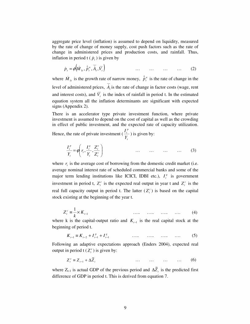
aggregate price level (inflation) is assumed to depend on liquidity, measured by the rate of change of money supply, cost push factors such as the rate of change in administered prices and production costs, and rainfall. Thus,

inflation in period t ( tp ) is given by

( )tt

a

ttt VApMp ,,ˆ,1 φ= … … … … (2)

where tM 1 is the growth rate of narrow money, a

tp is the rate of change in the

level of administered prices, tA is the rate of change in factor costs (wage, rent

and interest costs), and tV is the index of rainfall in period t. In the estimated

equation system all the inflation determinants are significant with expected signs (Appendix 2).

There is an accelerator type private investment function, where private investment is assumed to depend on the cost of capital as well as the crowding in effect of public investment, and the expected rate of capacity utilization.

Hence, the rate of private investment (t

pt

Y

I) is given by:

=

c

t

e

t

t

g

tt

t

p

t

Z

Z

Y

Ir

Y

I,,ϕ … … … … (3)

where tr is the average cost of borrowing from the domestic credit market (i.e.

average nominal interest rate of scheduled commercial banks and some of the

major term lending institutions like ICICI, IDBI etc.), g

tI is government

investment in period t, e

tZ is the expected real output in year t and c

tZ is the

real full capacity output in period t. The latter ( c

tZ ) is based on the capital

stock existing at the beginning of the year t.

….. ….. ….. …. (4)

where k is the capital-output ratio and 1−tK is the real capital stock at the

beginning of period t.

g

t

p

ttt IIKK 1121 −−−− ++≡ ….. ….. ….. …. (5)

Following an adaptive expectations approach (Enders 2004), expected real

output in period t ( e

tZ ) is given by:

ttet ZZZ

~1 ∆+≡ − … … … … (6)

where Zt-1 is actual GDP of the previous period and tZ~

∆ is the predicted first

difference of GDP in period t. This is derived from equation 7.

1

1−×≡ t

ct K

kZ

10

tZ~

∆ = f( 12

1, −− ∆∆ tt ZZ ) … … … … (7)

where 1−∆ tZ is the first difference of real output in the previous period and

12

−∆ tZ is the second difference of real output in the previous period. '

1−∆

tZ >0

& '2

1−∆

tZ <0. The r.h.s. determinants are all significant with expected signs in

the estimated equations (Appendix 2).

Government Block

Nominal aggregate government current expenditure ( tG ) is given by

)ˆ,( 1 ttt WGfG −= … … … … (8)

where tW is the revenue expenditure of government in period t, a policy

variable.

The level of government revenue (tax and non-tax) in period t is given by ( tT ):

1

1

ˆ−

−

×∆

×≡∆ t

t

tt T

Y

YT β … … … … (9)

where revenue buoyancy β is a policy determined variable. It is assumed that

government can set this through adjustments in tax rates and the administrative tax effort.

All government capital expenditure does not flow into investment and all public investment does not come from the government budget alone, since it is supplemented by investment of internal surpluses of public sector undertakings. However, the two are closely correlated. Hence, public investment is assumed to be a function of government capital expenditure:

… … … … (10)

where is the capital expenditure of government in period t, a policy variable. The r.h.s variables in behavioural equations (8) and (10) are all significant with expected signs in the estimated system of equations (Appendix 2).

The fiscal deficit in period t ( tF ) is given by

… … … (11)

)ˆ( gt

gt SI η=

gtS

gt

gt

gtt

gttt ODNTSWF ˆˆˆˆ ∆+≡−−+≡

11

where g

tD is the aggregate market borrowing of the government in period

t, gtN is non-debt capital receipts of the government (disinvestment etc.) and gtO∆ is the change in fiscal reserves.

External Block

The trade balance in terms of domestic currency in period t ( t

tB ) is given by

tt

t

t MXB −≡ … … … … (12)

where tX is the value of exports (including services) and tM is the value of

imports (including services) in period t.

Export demand was initially assumed to depend on the competitiveness of Indian products, measured by average tariffs as a proxy, the exchange rate, and the income of advanced countries, which account for the bulk of Indian exports. However, in the empirical estimation the exchange rate turned out to be insignificant. Hence, we have

( )a

ttt YUfX ,ˆ= … … … … (13)

where tU is the policy determined average tariff rate and a

tY is the GDP of

advanced countries, an exogenous variable.

The value of imports is assumed to depend on the exchange rate, the price of imported oil and oil related products, and domestic income. Hence,

( )t

o

ttt YPefM ,,= … … … … (14)

where te is the nominal exchange rate (Rs/US$), o

tP is the import price of oil

and petroleum products of Indian basket in terms of domestic currency, an exogenous variable, and Yt is nominal GDP in period t. The r.h.s. variables are significant with expected signs in the estimated equations (appendix 2).

The nominal exchange rate is assumed to be a function of the net inflow of foreign capital. Thus:

( )tt Jfe = … … … … (15)

where tJ is net foreign capital inflow. It has also been verified that other

variables such as the trade balance and interest rate do not have a significant effect on the exchange rate at present. The determinant is significant with expected sign in the estimated equation.

12

Net capital inflow tJ is assumed to be a function of the level of income in the

United States ( us

tY ), the major origin of foreign capital flows to India, and

China ( c

tY ), the main competing destination for these flows, and Indian GDP

( tY ) as a proxy for domestic demand.

),,( t

c

t

us

tt YYYfJ = … … … … (16)

It has been verified that capital inflow is not causally dependent on either the domestic-external interest rate differential or the exchange rate.

The net inflow of invisibles ( tL ) is assumed to be a function of aggregate

output of advanced (OECD) countries ( a

tY ) and the Middle East ( me

tY ), these

being the two major sources of remittances.

)( me

t

a

tt YYfL += … … … … (17)

The r.h.s arguments in equation 16 and 17 are all significant and have the expected signs.

The balance of payments identity in period t ( p

tB ) is given by

0≡∆+++≡ ttt

t

t

p

t RJLBB … … … … (18)

where tR∆ is the change in foreign exchange reserves.

Monetary Block

Narrow money ( tM 1 ) has been chosen as the estimate of money supply

instead of broad money because the money multiplier was found to be more stable for the former. Given the value of the money multiplier, the change in

narrow money supply in period t ( tM 1 ) is given by

)(1 tt HM γ= … … … … (19)

where tH is the change in high-powered money supply in period t . The

growth of high powered money ( tH ) is in turn assumed to be a function of

total government borrowing ( g

tD ) and change in foreign exchange reserves

( tR∆ ), i.e.,

),(1

t

g

t

t

t RDH

H∆=

−

λ

… … … … (20)

13

where 1−tH is the volume of high-powered money in the previous period.

Total government borrowing is given by

… … … … (21)

where g

tcD is government borrowing from RBI and gmtD is government

borrowing from the market.

Finally, the average nominal rate of interest is assumed to be a function of the rate of inflation, the policy rate and the volume of government borrowing from the market, the potential crowding out element7. Hence,

.… … … … (22)

where ti is the repo rate (bank rate before 2004-05) of RBI in period t. The

r.h.s variables are significant with expected signs in estimated equations (19), (20), and (22).

Variables of Interest

The key policy variables in solving this model include revenue and capital expenditure, tax buoyancy, the rate of change in administered prices, the policy interest rates, government borrowing from the market and (formerly) from RBI. The important exogenous variables include the growth of output in OECD countries as a group as well as in the USA, China, and the Middle East; world oil prices; and the rainfall index. A scenario is designed by setting the value of both the policy variables as well as the exogenous variables. The outcome variables of interest in each scenario include the growth rate, the inflation rate and the public debt-GDP ratio as well as some other key macroeconomic ratios, i.e., the investment rate; the trade deficit and current account deficit relative to GDP; the tax-GDP ratio, the revenue deficit-GDP ratio and the fiscal deficit-GDP ratio; and finally the exchange rate and interest rate.

Empirical Validation

The model has been estimated using annual data for the period 1991-92 to 2008-09, taking care of time series properties. The standard diagnostic tests have also been applied. The model has been solved for the sample period 2000-01 to 2008-09 and validated for this period. The root mean square

7 See, however, Palley (2002) and others of the ‘endogenous money’ school who maintain that money supply typically adjusts to satisfy money demand at the going rate of interest i.e. no crowding out.

g

mt

g

tc

g

t DDD ˆˆ +≡

)ˆ,ˆ,( gmtttt Dipr ξ=

14

percentage errors for all the key variables are shown in table 1. The tests show that the model is robust and performs well against actual outcomes for the sample period. Fig 1 shows the plots of estimated outcome variables against their actual values in the sample period. It is noted that the estimated model captures many though not all of the turning points in actual outcomes.

Table 1: Historical Validation of the Model

Description RMSPE Description RMSPE

Private Consumption 1.89 Net Capital Inflow 6.25

Government Consumption 1.58 Invisible (Remittances) 4.89

Govt. Current Expenditure 0.72 Rupee/US dollar exchange rate 2.16

Private Investment 2.43 Prime lending rate 1.00

Public Investment 3.67 Narrow Money Supply (M1) 2.49

Govt. Capital Expenditure 5.76 GDP Deflator 1.26

Total Govt. Revenue 1.54 Inflation (WPI) 6.80

Fiscal Deficit 1.35 Nominal output (factor cost) 1.15

Total Government Debt 3.03 Nominal output (market price) 1.35

Exports Including Services 1.15 Real output (factor cost) 0.28

Imports Including Services 1.66 Real output (market price) 0.61 Note: RMSPE=Root Mean Square Percentage Error (model generated)

15

Figure 1

16

4. A Proposed Fiscal Consolidation Program

The model developed above has been applied to assess the macro economic consequences of a fiscal consolidation program that eliminates the combined revenue deficit of the federal and state governments by the year 2014-15. This is the base case and the basic strategy. Two more scenarios are then examined to test the robustness of outcomes in the base case. An optimistic case where the rates of growth of the advanced countries are assumed to be 50% higher than those forecast by the IMF, and a pessimistic case of ‘double-dip’ recession where the rates of growth of USA and other advanced countries are assumed to fall to (-)1% and 0% in 2010-11 and 2011-12 respectively, and then gradually recover to the IMF forecast rate of 2.6% by the terminal year 2014-15. All other specifications are the same in these two cases as in the base case.

The Base Case

The outcomes resulting from a basic fiscal strategy of gradually eliminating the revenue deficit by 2014-15 have been first estimated for the base case, which is defined by the following assumptions:

1. In the real sector the output-capital ratio is assumed to remain constant at its current level of 0.375 and factor costs are assumed to rise at the rate of 4% per year. Administered prices are assumed to rise at the rate of 5% per year through the reference period.

2. In the monetary field, the policy(repo) rate has been held constant at 6%

3. In the external sector the base case assumes that the advanced countries, India’s major trading partners and important sources of remittances, will grow at the rates forecast by the IMF. USA, China and the Middle East, respectively the main source of foreign capital, the main competing destination of foreign capital, and one of the major sources of remittances, are also assumed to grow at the rate forecast by the IMF. The import weighted average tariffs are assumed to remain at the same level as at present, i.e., 9%. The weighted average price of the Indian basket of petroleum, oil and lubricant products have been assumed to remain at the same level for the reference period as the average price recorded for the period 2006-07 to 2008-09.

4. The largest set of assumptions relate to the fiscal block. On the revenue side, after smoothening the recent spurt in corporate and income tax buoyancy, it is assumed that there will be no major policy or performance changes affecting revenue collection, implying that revenue buoyancy remains unchanged at its medium term level of

17

1.225.8 On the expenditure side, nominal public investment is assumed to increase at 10% per year. It is also assumed that there will be no off-budget items for the reference period and that there will be no change in fiscal reserves during this period.

The impact on key macroeconomic outcomes of a gradual reduction in the combined revenue deficit of the centre plus states to zero by 2014-15 in this base case is shown in table 2.

Table 2: Base case outcomes 2010-11 to 2014-15 (%)

Year GDP

Growth WPI

Inflation Investment

Rate

Current A/c

Deficit-GDP Ratio

Fiscal Deficit-

GDP Ratio

Revenue Deficit-

GDP Ratio

Revenue-GDP Ratio

Public Debt-GDP Ratio

2010-11 8.1 7.6 33.7 2.7 10.3 5.9 21.1 75.0

2011-12 9.0 4.1 33.4 2.2 9.0 4.4 21.3 75.1

2012-13 9.2 4.2 34.0 2.4 7.6 3.0 21.5 73.6

2013-14 9.3 4.0 35.1 2.8 6.1 1.5 21.7 70.8

2014-15 8.4 4.0 36.3 3.4 5.9 0.0 21.8 68.8

In this scenario, the current account deficit rises to about 3.2% of GDP by 2014-15 and inflation remains moderate at just over 4%, except for a spike to 7.6% in the initial year. This is essentially the ‘base effect’ of a very low inflation rate in 2009-10. The revenue - GDP ratio is estimated at around 21.8%. The combined fiscal deficit of the centre and states as a ratio of GDP declines to about 6% by 2014-15 as the revenue deficit shrinks to zero (by assumption), implying government capital expenditure of around 6% of GDP in the terminal year. The corresponding public debt - GDP ratio is estimated at about 67.5%, which is quite reasonable compared to international benchmarks9. Based on these estimates, the 13th Finance Commission set a target of reducing the public debt to GDP ratio to 68% by 2014-15. This was subsequently incorporated in the fiscal consolidation programme introduced by the Central Government in the 2010-11 budget.

8 This assumption will clearly have to be revised following the adoption of a new direct taxes code and the introduction of Goods and Services Tax (GST). The impact of these major expected reforms of the tax system on revenue buoyancy could be significant but cannot be estimated at present. 9 There is no theoretically robust rule about the level of sustainable public debt. For a compelling analysis of the limitations of the Domar rule and other attempts to derive a general rule for sustainable debt see Rakshit (2005).

18

The most interesting implication of these results is that a strategy of compressing the revenue deficit down to zero creates the space for government capital expenditure of around 6% of GDP, leading to a high public investment rate. The crowding-in effect translates this to high private investment and an impressive total investment rate of over 36% of GDP by 2014-15. It is this high investment rate that largely accounts for the estimated high growth rate of over 8.5% through most of the reference period. An important concern is that the current account balance is likely to worsen in future since India may continue to grow at a faster rate than its major trading partners.

Alternative Scenarios

The robustness of these outcomes are tested under two alternative scenarios with optimistic and pessimistic assumptions regarding the external growth environment. These alternative assumptions are important because growth of the advanced countries drives the growth of Indian exports, with knock-on effects on overall growth. The optimistic scenario assumes 50% higher growth compared to the base case in the advanced countries.

Table 3: High advanced country growth outcomes 2010-11 to 2014-15 (%)

Year GDP

Growth WPI

Inflation Investment

Rate

Current A/c

Deficit-GDP Ratio

Fiscal Deficit-

GDP Ratio

Revenue Deficit-

GDP Ratio

Revenue-GDP Ratio

Public Debt-GDP Ratio

2010-11 8.1 7.6 33.7 2.7 10.3 5.9 21.1 75.0

2011-12 9.6 4.1 33.3 2.0 9.0 4.4 21.3 74.6

2012-13 10.0 4.2 33.9 2.0 7.6 3.0 21.6 72.7

2013-14 10.2 4.1 34.9 2.2 6.2 1.5 21.9 69.5

2014-15 9.2 4.0 36.1 2.9 5.9 0.0 22.1 67.2

The main change in outcomes in this case, compared to the base case, is that the growth rate is higher, reaching 10% in two years of the reference period. Inflation remains modest at around 4% except in 2010-11 as in the base case. On the fiscal side the revenue-GDP ratio improves marginally, while the fiscal deficit declines to less than 6% by 2014-15. The public debt-GDP ratio declines to 67%. On the external front, the current account deficit remains below 3% of GDP.

19

Table 4: Low advanced country growth outcomes 2010-11 to 2014-15 (%)

Year GDP

Growth WPI

Inflation Investment

Rate

Current A/c

Deficit-GDP Ratio

Fiscal Deficit-

GDP Ratio

Revenue Deficit-

GDP Ratio

Revenue-GDP Ratio

Public Debt-GDP Ratio

2010-11 7.6 7.6 33.3 2.9 10.3 5.9 21.8 75.4

2011-12 7.6 4.1 33.8 2.8 8.9 4.4 21.2 76.3

2012-13 7.8 4.1 33.5 3.2 7.5 3.0 21.2 75.4

2013-14 8.2 4.0 34.3 3.5 6.1 1.5 21.4 73.1

2014-15 7.9 4.0 35.3 3.9 5.9 0.0 21.5 71.0

In the pessimistic scenario ‘double-dip’ recession is assumed with growth rates of the advanced countries, including USA, falling to (-)1% in 2010-11, followed by 0% in 2011-12 and then gradually approaching the IMF forecast growth rate by 2014-15. In this case growth is slightly lower compared to the base case, but still impressive at over 7.5%. Inflation remains modest after the initial spike in 2010-11 as in the base case. The revenue-GDP ratio remains around 21.5% and the fiscal deficit declines to less than 6% by the end of 2014-15. The public debt-GDP ratio also declines, but remains higher than in the base case. The current account deficit reaches almost 4% of GDP and this is the main factor accounting for the lower rate of growth compared to the base case.

5. Conclusion

In this paper a fiscal consolidation program has been presented based on a policy simulation model. The exercise shows that it is possible to have such consolidation while at the same time maintaining high growth rates of around 8% or more. The strategy is to gradually bring down the revenue deficit to zero by 2014-15, while allowing a combined fiscal deficit for centre plus states of about 6% of GDP. This provides the space for substantial government capital expenditure, which translates to a significant public investment program. This leads in turn to high overall investment directly and indirectly, via the net ‘crowding in’ effect on private investment. High GDP growth follows through various stages of the Keynes-Kahn multiplier. On the fiscal side, the fiscal deficit ratio declines despite rising public expenditure because of the combined effect of the strong income multiplier for government capital expenditure (Das, 2007) and an estimated revenue buoyancy significantly greater than one.

The exercise has also tested the robustness of this strategy under alternative scenarios of higher and lower advanced country growth. Though this leads to

20

some variation in the rates of growth, fiscal deficit, public debt-GDP ratio, etc. the basic qualitative results of the fiscal consolidation strategy are sustained. It is also noted that the current account deficit varies between 2% to 4% of GDP in the alternative scenarios.

Elimination of the revenue deficit by 2014-15 will entail determined action both on the revenue side as well as in government expenditure. On the revenue side, maintaining high tax buoyancy following the envisaged reform in direct and indirect taxes will be key. Pending such reforms, substantial mobilization of non-tax revenues and non-debt capital receipts will be important in the short run. On the expenditure side the Government needs to focus on measures to contain revenue expenditure growth and create the space for robust capital expenditure. The risk is that if these steps on the revenue or expenditure side turn out to be politically or administratively infeasible, then the proposed fiscal consolidation program could fail.

21

References

Anand Rahul, Shanaka Peiris, and Magnus Saxegaard, 2010. “An estimated Model with Macrofinancial Linkages”, IMF Working paper no WP/10/21

Batini, Nicoletta, Vasco Gabril, Paul Levine and, Joseph Pearlman 2010. “A Floating Versus Managed Rate Regime in A DSGE Model of India”, NIPFP Working Paper, April, 10.

Bhaduri, Amit, 1990. Macroeconomics: The Dynamics of Commodity Production, Macmillan Education (UK).

Bhanumurthy N. R. and Lokendra Kumawat, 2009. “External Shocks and the Indian Economy: Analyzing through a Small, Structural Quarterly Macroeconometric Model”, MPRA Paper No. 19776, Online at http://mpra.ub.uni-muenchen.de/19776/ November.

Buchanan, James M. & Gordon Tullock, 1962. The Calculus of Consent, Ann Arbor, MI: University of Michigan Press.

Das, Surajit, 2007. “On Bringing Down the Fiscal Deficit”, Economic & Political Weekly, Vol.42, No.23, pp. 1638-1640, May.

Dixit, Avinash, 1996. The Making of Economic Policy: A Transaction Cost Politics Perspective, Munich Lectures in Economics, The MIT Press.

Dutt Amitava Krishna and Ross Jaime (ed) 2003. Developing Economies and structural Macroeconomics: Essays in Honour of Lance Taylor, Cheltenham, United Kingdom: Ewar Elgar.

Enders, Walter, 2004. Applied Econometric Time Series, John Wiley & Sons, New Delhi.

Friedman, Milton & Anna J. Schwartz, 1971. A Monetary History of the United States 1867-1960, Princeton University Press.

Gali, Jordi, 2008. Monetary Policy, Inflation, and the Business Cycle, Princeton University Press, Princeton.

Hicks, J.R., 1937. “Mr. Keynes and the Classics: A Suggested Interpretation”, Econometrica, Volume 5, No. 2, pp 147-159.

Kahneman, Daniel, 2003. “Map of Bounded Rationality: Psychology of Behavioural Economics”, American Economic Review, 93(5) 1441-1475.

Kahneman, Daniel and Amos Tversky, 1979. “Prospect Theory: An Analysis of Decision Making Under Risk”, Econometrica XLVII; 263-291.

22

Klein, L. R. and A. S. Goldberger (1955) An Econometric Model of the United States 1929-1952, Amsterdam, North-Holland.

Krishnamurthy, K., 2008. “Macroeconometric Models for India: Past, Present and Future”, in (eds.) Pandit, V and K R Shanmugam, Theory, Measurement and Policy: Evolving Themes in Quantitative Economics, Academic Foundation, New Delhi.

Kydland, Fyn E. and Edward C. Prescott, 1997 “Rules rather than Discretion: The Inconsistency of Optimal Plans”, Journal of Political Economy, 85, 473-491.

Lucas, Robert, E. Jr., 1976. “Econometric Policy Evaluation: A critique” in K. Brunner and A. Metzler (ed.) The Philips Curve and Labour Markets, Carnegie—Rochester Conference Series on Public Policy, 1 (Amsterdam: North Holland) 19—46.

Mishkin, Fredrick, 1995. “The Rational Expectations Revolution: A Review Article of Preston and Miller (ed.) The Rational Expectations Revolution: Readings from the Frontline”, NBER Working Paper No. 5043, February.

Mundle, Sudipto & Hiranya Mukhopadhyay, 1993. “Stabilization and the Control of Central Government Expenditure in India” in Pranab Bardhan, Mrinal Datta-Chaudhuri, T.N. Krishnan (ed.) Development and Change: Essays in Honour of K. N. Raj, Oxford University Press, Bombay.

Naastepad, C.W.M., 1999. The Budget Deficit and Macroeconomic Performance, Oxford University Press, New Delhi.

North, Douglass C., 1990. Institutions, Institutional Change, and Economic Performance. New York: Cambridge University Press.

Palley, Thomas I., 2002. “Endogenous Money: What It Is and Why It Matters”, Metroeconomica, 53:2, 152-180.

Persson, Torsten & Guido Tabellini, 1994. (eds.) Monetary and Fiscal Policy: Volume II: Politics, Cambridge, MA: MIT Press.

Rakshit, Mihir, 2005. “Budget Deficit: Sustainability, Solvency, and Optimality”, in (eds.) A. Bagchi Readings in Public Finance, Oxford University Press, New Delhi.

Simon, Herbert, 1957. “A Behavioural Model of Rational Choice”, in Models of Man, Social and Rational: Mathematical Essays in Rational Human Behaviour in a Social Setting, Wiley: New York.

Sims, Christopher A., 1980. “Macroeconomics and Reality”, Econometrica, 48:1, 1-48, January.

Taylor, Lance, 2004. Reconstructing Macroeconomics Structuralist Proposals and a Critique of the Mainstream, Harvard University Press.

23

Tinbergen, J., 1967. Economic Policy: Principles and Design, Amsterdam, North Holland.

Williamson, Oliver, 1985. The Economic Institutions of capitalism. New York: Free Press.

24

Appendix 1: Data Sources

ADEBT is the accumulated combined aggregate liability of the centre and state governments. Data from Handbook of Statistics on the Indian Economy, RBI.

ADVGDP is the index number of GDP of all advanced countries taken together (1970=100). Data from the World Economic Outlook, 2009, IMF.

AINF is the WPI based inflation for commodities with prices that are largely administered. Data from Office of the Economic Advisor, Ministry of Commerce & Industry, GOI.

CAPINFLOW is the net foreign capital inflow to India. Data from the Handbook of Statistics on Indian Economy, RBI.

CAPSTOCK is the net capital stock at 1999-2000 prices available at the beginning of any period. Data from the National Accounts Statistics , CSO, GOI.

CAPSTOCK is the net capital stock in the beginning of the period. Data from the National Account Statistics (NAS), CSO, GoI.

CHINAGDP is the index number of GDP of China (1970=100). Data from the World Economic Outlook, 2009, IMF.

CPR and CPU are respectively private final consumption expenditure and government final consumption expenditure. Data from National Accounts Statistics, CSO, GOI.

DUTY is the import weighted tariff rate. Data from website of the Planning Commission of India.

ECAP is the current price combined capital expenditure of the central and the state governments together. Data from Indian Public Finance Statistics, Ministry of Finance, GOI.

ECURR is the combined revenue expenditure of the central and state governments. Data from Indian Public Finance Statistics, Ministry of Finance, GOI.

ER is the exchange rate (Indian rupee per US$). Data from the Handbook of Statistics on Indian Economy, RBI.

FD is the combined fiscal deficit of the central and state governments. Data from Indian Public Finance Statistics, Ministry of Finance, GOI.

FOREX is the foreign exchange reserves. Data from Handbook of Statistics on Indian Economy, RBI.

GCP is the growth rate of wages, rents and interest cost in organized sector manufacturing industries in India. Data from Annual Survey of Industries (ASI), GOI as reported in the Handbook of Statistics on Indian Economy, RBI.

25

GDPCAPRATIO is the 3-year moving average of the ratio of GDP at factor cost constant price to net capital stock at constant prices. Data for both variables from National Accounts Statistics, CSO, GOI.

GM3 and GM0 are the annual growth rates of broad and high powered money supply respectively. Data from the Handbook of Statistics on Indian Economy, RBI.

GPWPI is the WPI based inflation of all commodities. Data from Office of the Economic Advisor, Ministry of Commerce & Industry, GOI.

INVISIBBLE is net invisible earnings, less earnings in services, in rupees crore. Data from the Handbook of Statistics on Indian Economy, RBI.

IPV and IPU are respectively gross private domestic capital formation, and gross domestic capital formation by the public sector. Data from National Accounts Statistics, CSO, GOI.

MB is the aggregate market borrowing of the Government. Data from Handbook of Statistics on the Indian Economy, RBI.

MEGDP is the index number of GDP of Middle East countries taken together (1970=100). Data from the World Economic Outlook, 2009, IMF.

MTO is the imports including services. Data from Handbook of Statistics on Indian Economy, RBI.

NDCR is the non debt capital receipts of the government comprising dis-investment etc. Data from Indian Public Finance Statistics, Ministry of Finance, GOI.

OIL is the index number of international price of oil and petroleum products of the Indian basket in terms of rupees crore (1972-73 = 100). Data from the Handbook of Statistics on Indian Economy, RBI.

PLR is the average nominal (simple) prime lending rate calculated as the average RBI prescribed lending rate of all scheduled commercial banks including SBI and prime lending rates of term lending institutions like IDBI, IFCI, ICICI, IIBI/IRBI and that of SFCs. Handbook of Statistics on Indian Economy, RBI.

RAIN is the rainfall index for India is taken from NASA website.

RD is the combined revenue deficit of the central and state governments. Data from Indian Public Finance Statistics, Ministry of Finance, GOI.

REPO is the RBI determined bank rate taken up to 2003-04 and repo rate thereafter. Data from Handbook of Statistics on Indian Economy, RBI.

TAX is combined revenue receipts of the central and state governments. Data from Indian Public Finance Statistics, Ministry of Finance, GOI.

TD is the trade deficit. Data from Handbook of Statistics on Indian Economy, RBI.

26

USGDP is the index number of GDP of USA. Data from the World Economic Outlook, 2009, IMF.

XTO is the exports including services. Data from Handbook of Statistics on Indian Economy, RBI.

YMP, ZYMP, YF and ZYF are respectively GDP at current market prices, GDP at constant (1999-2000) prices, GDP at factor cost in current prices, and GDP at factor cost in constant (1999-2000) prices. Data from National Accounts Statistics, CSO, GOI.

DUMCRISIS takes 1 for 2008-09 to capture the impact of global financial crisis and 0 for rest of the period.

Dummy variables have been introduced in many of the equations largely to take care of the structural shifts and also the outliers in the estimated equations.

AR (Auto Regression) and MA (Moving Average) terms have been used to control the presence of autocorrelation in the estimated equations.

27

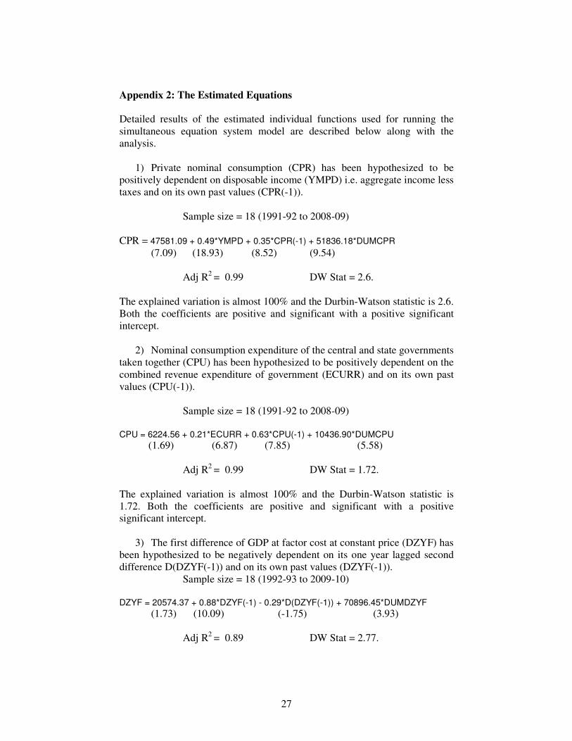
Appendix 2: The Estimated Equations Detailed results of the estimated individual functions used for running the simultaneous equation system model are described below along with the analysis.

1) Private nominal consumption (CPR) has been hypothesized to be positively dependent on disposable income (YMPD) i.e. aggregate income less taxes and on its own past values (CPR(-1)).

Sample size = 18 (1991-92 to 2008-09)

CPR = 47581.09 + 0.49*YMPD + 0.35*CPR(-1) + 51836.18*DUMCPR

(7.09) (18.93) (8.52) (9.54) Adj R2 = 0.99 DW Stat = 2.6.

The explained variation is almost 100% and the Durbin-Watson statistic is 2.6. Both the coefficients are positive and significant with a positive significant intercept.

2) Nominal consumption expenditure of the central and state governments taken together (CPU) has been hypothesized to be positively dependent on the combined revenue expenditure of government (ECURR) and on its own past values (CPU(-1)).

Sample size = 18 (1991-92 to 2008-09)

CPU = 6224.56 + 0.21*ECURR + 0.63*CPU(-1) + 10436.90*DUMCPU

(1.69) (6.87) (7.85) (5.58) Adj R2 = 0.99 DW Stat = 1.72.

The explained variation is almost 100% and the Durbin-Watson statistic is 1.72. Both the coefficients are positive and significant with a positive significant intercept.

3) The first difference of GDP at factor cost at constant price (DZYF) has been hypothesized to be negatively dependent on its one year lagged second difference D(DZYF(-1)) and on its own past values (DZYF(-1)).

Sample size = 18 (1992-93 to 2009-10)

DZYF = 20574.37 + 0.88*DZYF(-1) - 0.29*D(DZYF(-1)) + 70896.45*DUMDZYF

(1.73) (10.09) (-1.75) (3.93) Adj R2 = 0.89 DW Stat = 2.77.

28

The explained variation is 89% and the Durbin-Watson statistic is 2.77. The coefficient of one year lagged second difference is negative and insignificant while the coefficient of one year lag of the dependent variable is positive and significant with a positive significant intercept.

4) Investment by the government and public sector enterprises (IPU) has been hypothesized to be positively dependent on combined capital expenditure of government (ECAP) and on its own past values (IPU(-1)).

Sample size = 15 (1994-95 to 2008-09)

IPU = 7322.92 + 0.83*ECAP + 0.62*IPU(-1) + 17221.93*DUMIPU

(2.49) (11.81) (11.31) (5.07) Adj R2 = 0.99 DW Stat = 2.43.

The explained variation is almost 100% and the Durbin-Watson statistic is 2.43. Both the coefficients are positive and significant with a positive significant intercept.

5) The private investment to GDP ratio (IPV/YF) has been hypothesized to be negatively dependent upon the average prime lending rate and positively dependent on the ratio of expected real output to full capacity real output (RATIO) and the government investment rate (IPU/YF).

Sample size = 18 (1991-92 to 2008-09)

IPV/YF = -0.69 - 0.01*PLR + 0.93*RATIO + 0.53*(IPU/YF) + 0.07*DUMIPV + 0.01*DUMCRISIS (-18.97) (-21.22) (30.02) (4.21) (24.25) (3.66)

Adj R2 = 0.99 DW Stat = 2.87.

The explained variation is almost 100% and the Durbin-Watson statistic is 2.87. All the coefficients are significant with a negative significant intercept. We have added a crisis dummy here following the ‘financial crisis’ of developed World.

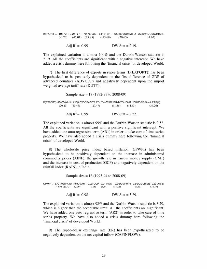
6) The value of imports in rupee terms (IMPORT) has been hypothesized to be positively dependent on GDP at factor cost (YF) and the average international price of oil and petroleum products in the Indian basket (OIL) and negatively dependent upon the average rupee-dollar exchange rate (ER).

Sample size = 17 (1992-93 to 2008-09)

29

IMPORT = -10372 + 0.24*YF + 79.76*OIL - 6117*ER + 42936*DUMMTO - 27395*DUMCRISIS (-0.73) (45.01) (25.85) (-13.69) (20.65) (-4.62)

Adj R2 = 0.99 DW Stat = 2.19.

The explained variation is almost 100% and the Durbin-Watson statistic is 2.19. All the coefficients are significant with a negative intercept. We have added a crisis dummy here following the ‘financial crisis’ of developed World.

7) The first difference of exports in rupee terms (D(EXPORT)) has been hypothesized to be positively dependent on the first difference of GDP of advanced countries (ADVGDP) and negatively dependent upon the import weighted average tariff rate (DUTY).

Sample size = 17 (1992-93 to 2008-09)

D(EXPORT)=174058+8111.6*D(ADVGDP)-7170.3*DUTY+53598*DUMXTO-108671*DUMCRISIS + 0.5*AR(1)

(20.29) (10.46) (-20.47) (11.56) (14.43) (36.26)

Adj R2 = 0.99 DW Stat = 2.52.

The explained variation is almost 99% and the Durbin-Watson statistic is 2.52. All the coefficients are significant with a positive significant intercept. We have added one auto regressive term (AR1) in order to take care of time series property. We have also added a crisis dummy here following the ‘financial crisis’ of developed World.

8) The wholesale price index based inflation (GPWPI) has been hypothesized to be positively dependent on the increase in administered commodity prices (AINF), the growth rate in narrow money supply (GM1) and the increase in cost of production (GCP) and negatively dependent on the rainfall index (RAIN) in India.

Sample size = 16 (1993-94 to 2008-09)

GPWPI = -5.79 +0.21*AINF +0.09*GM1 +0.02*GCP +0.01*RAIN +2.3*DUMPWPI +2.8*DUMCRISIS+0.63*AR(2) (-4.67) (11.43) (2.99) (1.88) (5.34) (14.28) (7.40) (14.37)

Adj R2 = 0.98 DW Stat = 3.29.

The explained variation is almost 98% and the Durbin-Watson statistic is 3.29, which is higher than the acceptable limit. All the coefficients are significant. We have added one auto regressive term (AR2) in order to take care of time series property. We have also added a crisis dummy here following the ‘financial crisis’ of developed World.

9) The rupee-dollar exchange rate (ER) has been hypothesized to be negatively dependent on the net capital inflow (CAPINFLOW).

30

Sample size = 14 (1995-96 to 2008-09)

ER = 45.91 - 3.61e-05*CAPINFLOW + 6.45DUMER +1.52*AR(1)-0.63*AR(2)

(27.16) (-13.95) (5.47) (10.55) (-5.00) Adj R2 = 0.99 DW Stat = 1.50.

The explained variation is almost 100% and the Durbin-Watson statistic is 1.5. The coefficient is negative significant with a positive significant intercept. We have added two auto regressive terms (AR1 & AR2) in order to take care of time series property.

10) The net capital inflow (CAPINFLOW) has been assumed to be a function of GDP of China (CHINAGDP) that of United States (USGDP) and Indian domestic real GDP (ZYMP) at market price.

Sample size = 18 (1991-92 to 2008-09)

CAPINFLOW = -144320 - 20.6*CHINAGDP + 11.7*USGDP + 0.08*ZYMP + (-3.30) (-1.58) (2.59) (1.81) 181174.5*DUMCAP - 58039.2*DUMCRISIS (13.81) (-5.39)

Adj R2 = 0.99 DW Stat = 1.81.

The explained variation is almost 99% and the Durbin-Watson statistic is 1.81. The coefficients are significant with a negative significant intercept. We have added a crisis dummy here following the ‘financial crisis’ of developed World.

11) The net invisible flow of current account of balance of payment (INVISIBLE) has been hypothesized to be a function of joint GDP of the advanced countries (ADVGDP) and the Middle East (MEGDP).

Sample size = 17 (1992-93 to 2008-09)

INVISIBLE =-48600 +105.06*(MEGDP +ADVGDP) +16919.1*DUMINV +13575.6*DUMCRISIS +0.6AR(1) (-5.85) (17.10) (5.06) (2.79) (2.90)

Adj R2 = 0.99 DW Stat = 2.02. The explained variation is almost 99% and the Durbin-Watson statistic is 2.02. The coefficients are significant with a negative significant intercept. We have added a crisis dummy here following the ‘financial crisis’ of developed World. We have also added one auto regressive term (AR1) in order to take care of time series property.

31

12) The average prime lending rate (PLR) has been hypothesized to be positively dependent on the WPI inflation rate (GPWPI), the RBI determined repo rate (REPO) and the market borrowing of the government (MB).

Sample size = 14 (1995-96 to 2008-09)

PLR = 5.99 + 0.11*GPWPI + 0.77*REPO + 1.78e-06*MB + 0.75*DUMPLR

(37.18) (8.15) (55.75) (2.69) (17.04) Adj R2 = 0.99 DW Stat = 1.90.

The explained variation is almost 99% and the Durbin-Watson statistic is 1.90. The coefficients are significant with a positive significant intercept.

13) The inflation in GDP deflator (GPGDP) has been hypothesized to be positively dependent on the inflation based on WPI (GPWPI).

Sample size = 20 (1990-91 to 2009-10)

GPGDP = 0.14 + 0.98*GPWPI + 3.82*DUMPGDP

(0.35) (17.17) (10.18) Adj R2 = 0.94 DW Stat = 3.03.

The explained variation is almost 94% and the Durbin-Watson statistic is 3.03, which is higher than the acceptable level. The coefficient is significant with a positive intercept.

14) The narrow money (GM1) has been hypothesized to be positively dependent on the high-powered reserve money (GM0).

Sample size = 18 (1991-92 to 2008-09)

GM1 = -36346.31 + 1.37*M0 + 42635.34*DUMM1 - 81273.64*4DUMCRISIS

(-10.03) (136.95) (10.76) (-8.13) Adj R2 = 0.99 DW Stat = 2.50.

The explained variation is almost 99% and the Durbin-Watson statistic is 2.50. The coefficient is positive and significant with a negative significant intercept. We have added a crisis dummy here also following the ‘financial crisis’ of developed World.

15) The stock of reserve money (M0) has been hypothesized to be positively dependent on foreign exchange reserves (FOREX) and market borrowing by the government (MB).

32

Sample size = 18 (1991-92 to 2008-09)

M0 = 103854.76 - 0.43*FOREX + 0.98*MB + 64698.70*DUMGM0 + 115994.77*DUMCRISIS (17.64) (27.05) (8.49) (5.99) (7.44)

Adj R2 = 0.99 DW Stat = 1.98.

The explained variation is almost 100% and the Durbin-Watson statistic is 1.98. The coefficients are significant with a positive significant intercept. We have added a crisis dummy here also following the ‘financial crisis’ of developed World.

16) The combined revenue receipt of Central and State governments (TAX) has been hypothesized to be positively dependent on the GDP at nominal market price (YMP).

Sample size = 18 (1991-92 to 2008-09)

LOG(TAX) = -6.80 + 1.33*LOG(YMP) + 0.06*DUMTAX + 0.90*AR(1)

(-2.71) (8.74) (4.94) (17.06) Adj R2 = 0.99 DW Stat = 2.16.

The explained variation is almost 100% and the Durbin-Watson statistic is 2.16. The coefficient is significant with a negative significant intercept. We have added one auto regressive term (AR1) in order to take care of time series property.

17) The combined revenue expenditure of government (ECURR) has been hypothesized to be positively dependent on the nominal GDP at factor cost (GM0) and on its own past values.

Sample size = 18 (1991-92 to 2008-09)

ECURR = -4141.94 + 0.69*ECURR(-1) + 0.10*YF + 121621.23*DUMECURR +175815.36*DUMCRISIS

(-1.31) (13.42) (8.97) (6.06) (21.55)

Adj R2 = 0.99 DW Stat = 2.15. The explained variation is almost 100% and the Durbin-Watson statistic is 2.15. The coefficients are positive and significant with a negative intercept. We have added a crisis dummy here following the ‘financial crisis’ of developed World to capture the fiscal stimulus including the 6th pay commission impact.

33

18) The first difference of capital stock at the beginning of any period (CAPSTOCK) has been hypothesized to be positively dependent on the total investment of last period (i.e. private investment plus government investment IPV(-1)+IPU(-1)).

Sample size = 17 (1992-93 to 2008-09)

D(CAPSTOCK) = 80351.29 + 0.43*(IPV(-1)+IPU(-1)) + 137422.67*DUMCAPS

(9.87) (34.24) (5.61) Adj R2 = 0.99 DW Stat = 1.44.

The explained variation is 99% and the Durbin-Watson statistic is 1.44. The coefficient is significant with a positive significant intercept.

19) The constant price GDP at factor cost (ZYF) has been hypothesized to be positively dependent on GDP at constant market price (ZYMP).

Sample size = 19 (1991-92 to 2009-10)

ZYF = -27970.54 + 0.79*ZYMP + 0.16*ZYMP(-1)

(-4.77) (17.43) (3.15) Adj R2 = 0.99 DW Stat = 1.86.

The explained variation is almost 100% and the Durbin-Watson statistic is 1.86. The coefficient is significant with a negative significant intercept.

20) The market borrowing of the government (MB) has been hypothesized to be positively dependent on the fiscal deficit of last year (FD (-1).

Sample size = 16 (1993-94 to 2008-9)

MB = -22693.57 + 0.75*FD(-1) + 59681.33*DUMCRISIS + 57159.69*DUMMB

(-4.93) (23.84) (9.08) (9.73) Adj R2 = 0.98 DW Stat = 2.29.

The explained variation is 98% and the Durbin-Watson statistic is 2.29. The coefficient is significant with a negative significant intercept. We have added a crisis dummy here also due to fiscal stimulus following the ‘financial crisis’ of developed World.

34

Appendix 3: Definitions

Ratios to GDP (Yt):

t

tt

Y

DBDBG = … … (D1)

where, tDB is the accumulated debt.

t

tt

Y

RDRDG = … … (D2)

where, tRD is the revenue deficit.

t

tt

Y

FFDG = … … (D3)

where, tFD is the fiscal deficit.

t

t

tt

Y

BTDG = … … (D4)

where, t

tB is the balance of trade in goods and services.

t

tt

Y

TRG = … … (D5)

Where, tT is the combined revenue of Centre & States.

t

tt

Y

IIG = … … (D6)

Where, tI is the investment.

Growth Rates:

)1(10011

−×=−− t

t

t

t

Y

Y

Y

Y … … (D7)

)1(10011

−×=−− t

t

t

t

Z

Z

Z

Z … … (D8)

)1(10011

−×=−− t

t

t

t

H

H

H

H … … (D9)

)1(10011

−×=−− t

t

t

t

p

p

p

p … … (D10)